Multilevel Primary Aim Analyses of Clustered SMARTs:
With Applications in Health Policy

Abstract

Many health policies or programs can be conceptualized as adaptive interventions. An adaptive intervention is a sequence of decision rules that guide the provision of actions (intervention options) at critical decision points based on the evolving need of recipients, including their response to prior actions. In many health policy settings, adaptive interventions target a population of clusters (e.g., schools), with the ultimate intent of impacting outcomes at the level of individuals within the clusters (e.g., mental health care providers in the schools). Health policy researchers can use clustered, sequential, multiple assignment, randomized trials (SMARTs) to answer important scientific questions concerning clustered adaptive interventions. A common primary aim is to compare the mean of a nested, end-of-study outcome between two clustered adaptive interventions. However, existing methods are not suitable when the primary outcome in a clustered SMART is nested and longitudinal (e.g., repeated outcome measures nested within mental healthcare providers, and mental healthcare providers nested within schools). This manuscript proposes a three-level marginal mean modeling and estimation approach for comparing adaptive interventions in a clustered SMART. The proposed method enables policy analysts to answer a wider array of scientific questions in the marginal comparison of clustered adaptive interventions. Further, relative to using an existing two-level method with a nested, but non-longitudinal, end-of-study outcome, the proposed method benefits from improved statistical efficiency. With this approach, we examine longitudinal comparisons of adaptive interventions for improving school-based mental healthcare and contrast its performance with existing approaches for studying static (i.e., singly measured) end-of-study outcomes. Methods were motivated by the Adaptive School-Based Implementation of CBT (ASIC) study, a clustered SMART designed to construct an adaptive health policy to improve the adoption of evidence-based CBT by mental healthcare professionals in high schools across Michigan.

1 Introduction

Adaptive interventions, also known as dynamic treatment regimes, are protocols used to guide decision-making at critical decision points during intervention (Laber et al., 2014). This includes guidance on whether and when to modify (e.g., augment, intensify, or switch) the provision of intervention options, as well as what information should inform such decisions.

In health policy settings, intervention often targets a cluster of individuals. A cluster is defined as an intact group of individuals, often formed through naturally occurring organizational or administrative affiliations. For example, in an attempt to improve the behavior of clinicians (e.g., nurse-practitioners, doctors, or mental health providers), a health policy intervention may target hospitals. Doing so can address widespread barriers to patient wellbeing, as well as promote supportive organizational environments to foster development of medical professionals. We call such interventions (i.e., those that act on clusters of individuals but are designed to improve individual outcomes) clustered interventions. This manuscript concerns clustered adaptive interventions (cAIs); i.e., adaptive interventions for which the sequence of decision rules guiding intervention delivery is based on the baseline conditions and evolving needs of each pre-determined cluster of individuals (NeCamp et al., 2017). Like clustered interventions at large, a defining feature of cAIs is cluster-level action with the intent of impacting outcomes at the individual-level.

Such interventions have natural applications to public policy, as they leverage existing social structures (e.g., schools, hospitals, communities). Furthermore, cAIs are particularly useful in implementation science, which focuses on improving the adoption and fidelity of evidence-based interventions in real-world settings (Bauer and Kirchner, 2020). By leveraging pre-existing administrative clusters, such as schools and hospitals, cAIs can help address systemic barriers to effective implementation and support sustainable practice change (Kilbourne et al., 2014, 2018; Quanbeck et al., 2020).

Sequential, multiple assignment, randomized trials (SMARTs) form a class of experimental designs which act as valuable data collection tools for optimizing the construction of adaptive interventions. Through sequential randomization, SMARTs offer intervention designers an opportunity to analyze a multitude of questions concerning adaptive intervention construction (Nahum-Shani et al., 2012). Clustered SMARTs (cSMARTs) are a class of SMARTs which utilize cluster-level randomization and treatment, but for which the primary outcome is measured at the individual level. Subsequently, researchers can use cSMARTs to address important scientific questions preventing the construction of high quality clustered adaptive interventions. Scientists have employed cSMARTs in a wide variety of health application areas, including school-based healthcare (Kilbourne et al., 2018), mental health (Kilbourne et al., 2014), substance abuse (Quanbeck et al., 2020; Fernandez et al., 2020), and infectious disease prevention (Zhou et al., 2020).

A common primary aim in a SMART is the comparison of two (or more) adaptive interventions on the marginal mean of an end-of-study outcome (Nahum-Shani et al., 2012). The foundation of the statistical approach for this aim is rooted in the work of Orellana et al. (2010a, b); Robins et al. (2008). Lu et al. (2015) and Li (2016) developed analytic methods addressing this aim in the case of a continuous longitudinal outcome, with Seewald et al. (2020) presenting a sample size formula to power a SMART with such a primary aim. Additionally, Luers et al. (2019); Dziak et al. (2019) further explore more general methods for longitudinal outcome analyses in these settings.

SMART design and analyses generally remain active areas of statistical research (Artman et al., 2024; Wank et al., 2024). While these methodological advances have materially enhanced the design and analysis of individually randomized SMARTs, the literature on clustered SMARTs is still emerging. NeCamp et al. (2017) extended the standard approach to enable comparison of clustered adaptive interventions via the marginal mean of an end-of-study outcome, and developed a corresponding sample size formula. Additionally, Ghosh et al. (2015) proposed a similar sample size for binary end-of-study outcome comparison and Xu et al. (2019) extended these approaches for complex clustering structures. More recently, Pan et al. (2024+) developed finite sample adjustments unique to the analysis of clustered SMARTs. Beyond these contributions, however, research on clustered SMARTs remains sparse.

The primary methodological contribution of this manuscript is an approach for comparing the marginal mean of a longitudinal continuous outcome between two clustered adaptive interventions embedded in a cSMART. The nested structure of repeated observations within individuals within clusters induces multiple “levels” to consider in the analysis. In the analysis of cluster-randomized RCTs, such three-level analytic methods are commonplace (Teerenstra et al., 2010).

The proposed method combines methods for comparing adaptive interventions on a longitudinal outcome Lu et al. (2015); Li (2016); Seewald et al. (2020) with methods for comparing clustered adaptive interventions NeCamp et al. (2017); Pan et al. (2024+). The method offers two important benefits: First, most importantly, it enables the marginal mean comparison of cAIs on a longitudinal outcome, opening the door to a wider array of causal estimands concerning the dynamical effects of cAIs. Second, we provide empirical evidence that incorporating repeated measurements can help improve statistical efficiency even when the primary outcome of interest is a static end-of-study measure. Thus, analysts interested in the mean comparison of cAIs on an end-of-study outcome have greater statistical precision under the new approach. In many policy settings, the cost of collecting an additional research outcome for all clusters participating in the trial can outweigh the cost of recruiting an additional cluster, thus underscoring the importance of this advantage (Raudenbush, 1997; Rutterford et al., 2015).

Methods are illustrated using the Adaptive School-Based Implementation of CBT (ASIC) study, a clustered SMART that aims to improve the adoption of cognitive behavioral therapy (CBT), an evidence-based mental health treatment, in Michigan high schools. ASIC collected weekly measures of its primary outcome (quantity of CBT delivery) across 10 months (Kilbourne et al., 2018). We note that the proposed approach applies more broadly than two-stage, prototypical, clustered SMART designs such as ASIC’s. We discuss extension to more general settings in Appendix A7.

2 Motivating Example: ASIC

As discussed in Section 1, the Adaptive School-based Implementation of CBT (ASIC) study, a clustered SMART designed to study school-based mental healthcare, motivates our methods (Kilbourne et al., 2018).

In the United States, youths are, in general, more likely to receive mental health services from schools than from any other child-serving mental healthcare sector (Duong et al., 2020). Depression and anxiety disorders are the most common mental health disorders among American youths. While evidence-based practices (EBPs) such as cognitive behavioral therapy (CBT) can improve outcomes among these individuals, less than $20\%$ of young patients have access to EBPs. Furthermore, even when EBPs are offered, treatment fidelity can be weak (Kilbourne et al., 2018).

Recently, researchers at the University of Michigan conducted the ASIC study to inform the design of a two-stage clustered adaptive intervention aimed at addressing systemic barriers to CBT delivery in high schools. The scientists sought to create an adaptive intervention that combines three existing implementation strategy components for promoting CBT-uptake among school professionals (SPs, i.e., school employees tasked with delivering mental health services to students). The existing strategies were: (i) Replicating Effective Programs (REP), (ii) Coaching, and (iii) Facilitation. Based on research conducted prior to the ASIC study, REP and Coaching were designed for use in Stages 1 and 2 of implementation, whereas Facilitation was designed only for use in Stage 2 of implementation. The REP component includes a CBT uptake monitoring protocol that guides how implementation support professionals assess progress implementation. This monitoring protocol is used, for example, to determine whether a school is a “slower-responder” (also referred to as a “non-responder”) school at the end of Stage 1, i.e., eligible for Facilitation in Stage 2.

The ASIC study included 169 SPs across 94 Michigan high schools. All participating schools (i) had not previously participated in any school-based CBT implementation initiatives, (ii) were within two hour driving distance of a mental health professional trained to serve as a coach for the study, (iii) had at least one eligible SP that agreed to participate in study assessments, and (iv) had sufficient resources to allow for delivery of individual and/or group mental health support on school grounds (Smith et al., 2022).

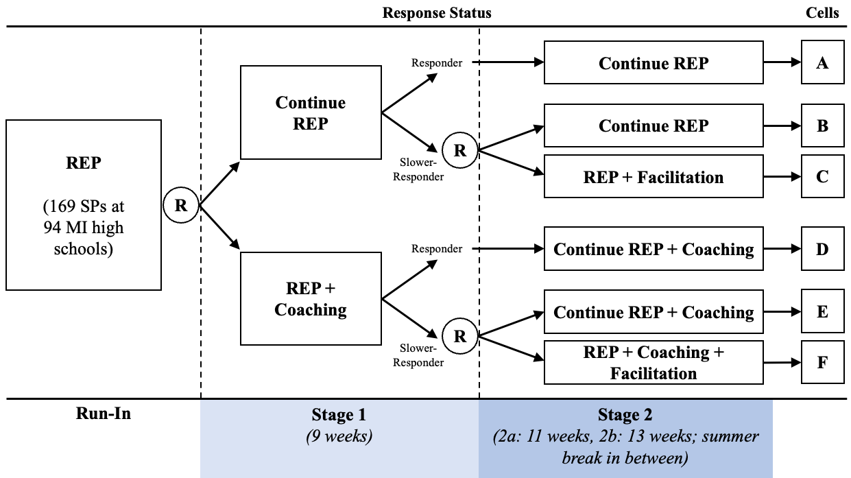
Figure 1: ASIC Structure

Figure 1 shows ASIC’s randomization structure. During a three month run-in stage, all 94 schools were offered REP. After this phase, schools were randomized to either continue REP, or to augment REP with Coaching. Nine weeks after this initial randomization, schools deemed “slower-responders” were re-randomized to either augment with their first stage intervention with Facilitation or continue with their initial treatment. Response status was a function of SP-reported barriers and frequency of CBT delivery, aggregated to the level of the school; see Smith et al. (2022) for a precise definition.

The primary research outcome is weekly measurements of CBT delivery by each SP (Kilbourne et al., 2018). The nesting of repeated measures outcomes (weekly CBT delivery) within each SP, and the nesting of multiple SPs within each school induces the three-level clustering structure (outcomes nested within SPs nested within schools) that is central to the method developed in this manuscript.

As discussed in greater detail in Section 3.2, most clustered SMARTs contain a set of embedded cAIs. By design, ASIC includes four such embedded cAIs (see Table 1); and ASIC’s primary aim was to study the difference in the marginal expectation of total CBT delivery at the end of implementation under the most versus least intensive of the four cAIs (Kilbourne et al., 2018). As demonstrated in the simulation experiments of Section 8.2, and illustrated in Section 7, the proposed repeated measures (longitudinal) data analytic method enhances precision and reliability in addressing such primary aims. Additionally, in the illustrative data analyses, we show how the method can be used to answer new scientific questions using the weekly outcome measurements (e.g., to compare the four embedded cAIs in terms of changes in SP-level CBT delivery trajectories over time) otherwise masked in a static end-of-study analysis.

3 Clustered SMARTs with Repeated Measures

SMARTs are a class of multi-stage, factorial randomized trial designs, which leverage sequential randomization to inform the construction of optimal adaptive interventions (Nahum-Shani and Almirall, 2019). SMART designs can vary widely; the characterizing feature of a SMART is that at least some units are randomized more than once (Seewald et al., 2021).

As discussed in Section 1, clustered SMARTs (cSMARTs) can inform the optimal construction of clustered adaptive interventions (NeCamp et al., 2017). In a cSMART, clusters of individuals are sequentially randomized, with outcomes primarily measured with respect to individuals. For example, ASIC trial designers randomized entire schools with the intent to study outcomes at the SP-level (Kilbourne et al., 2018). While cSMARTs typically randomize groups of humans, this need not be the case in general. Xu et al. (2019) provides an example of a cSMART studying dental procedures in which each humans subject represents a cluster, with their teeth representing the individuals.

3.1 SMART Randomization Structures

Figure 2 displays four common SMART “design types.” In each of the presented design types, all clusters are randomized to one of two first stage intervention options; however, the design types differ in their re-randomization structure. SMART designs I, II, and III incorporate an embedded binary tailoring variable, “response.” SMART design IV (often called an “unrestricted $2\times 2$ SMART,”) differs from the other three in this respect, as all clusters that received a given first-stage intervention are re-randomized to one of two second-stage interventions. This re-randomization is restricted to non-responders in SMART design II, with SMART design III further restricting re-randomization to non-responders of a single first-stage treatment arm. SMART design II is possibly the most common SMART design, and is often referred to as a “prototypical” SMART.

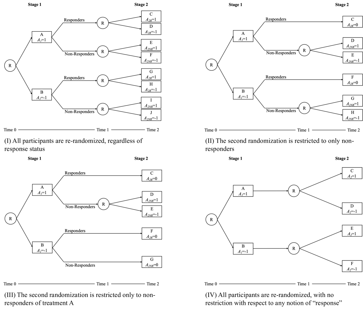
Figure 2: Illustrative SMART Structure Examples

SMART design I, while not yet employed in the clustered setting, is popular in individually randomized SMARTs (e.g., Oslin (2005)). Kilbourne et al. (2014) details the first documented clustered SMART, employing SMART design III above. Quanbeck et al. (2020) employed SMART design IV to study implementation strategies to promote concordant opioid prescription. Furthermore, while all four design types above use two stages of binary randomization, this need not be the case for all SMARTs — see Xu et al. (2019) for a clustered SMART with four-arm re-randomization for non-responding clusters.

As shown in Figure 1, ASIC was a prototypical SMART. As such, we will use this design to illustrate and motivate notation and methods throughout the remainder of the main body of this manuscript. Appendix A7 discusses generalizations to other SMART structures.

3.2 Embedded Adaptive Interventions

A clustered adaptive intervention is a sequence of decision rules guiding the provision of intervention based on the baseline and changing status of recipient clusters. cSMART designs contain a notion of embedded cAIs; i.e., protocolized decision rules embedded in their design. Prototypical SMARTs contain four embedded adaptive interventions, indexed by choice of first-stage intervention, second-stage treatment for responders, and second-stage treatment for non-responders. I.e., we can identify a given embedded adaptive intervention for prototypical SMARTs as the triple $(a_{1},a_{2R},a_{2NR})$, where $a_{1}$ represents choice of first-stage intervention, and $a_{2R}/a_{2NR}$ represent choice of second-stage intervention for responders/non-responders. Given prototypical SMARTs do not re-randomize responders, the choice of first-stage treatment and second-stage treatment for non-responders induces the four embedded adaptive interventions. For brevity, embedded adaptive interventions in prototypical SMARTs are often denoted as a double $(a_{1},a_{2NR})$. As such, we can denote the ASIC embedded cAIs as (i) (REP+Coaching, Facilitation), (ii) (REP+Coaching, No Facilitation), (iii) (REP, Facilitation), (iv) (REP, No Facilitation). ASIC’s primary aim comparison involved the total CBT delivery under (REP+Coaching, Facilitation) and (REP, No Facilitation). Table 1 below illustrates these four embedded cAIs.

By convention, we let $\mathcal{D}$ denote the set of embedded cAIs in a clustered SMART (Seewald et al., 2020). Using standard $\pm 1$ notation for treatment indicators, this corresponds to $\mathcal{D}:=\left\{(1,1),(1,-1),(-1,1),(-1,-1)\right\}$ for prototypical cSMARTs.

cAI$(a_{1},a_{2NR})$	First-Stage Intervention	School Response	Second-Stage Intervention	Cells in Fig. 1
cAI$\left(1,1\right)$	REP + Coaching ($A_{1}=1$)	Responder ($R=1$)	Continue REP + Coaching	D
		Non-responder ($R=0$)	Add Facilitation ($A_{2NR}=1$)	F
cAI$\left(1,-1\right)$	REP + Coaching ($A_{1}=1$)	Responder ($R=1$)	Continue REP + Coaching	D
		Non-responder ($R=0$)	Continue REP + Coaching ($A_{2NR}=-1$)	E
cAI$\left(-1,1\right)$	REP Only ($A_{1}=-1$)	Responder ($R=1$)	Continue REP	A
		Non-responder ($R=0$)	Add Facilitation ($A_{2NR}=1$)	C
cAI$\left(-1,-1\right)$	REP Only ($A_{1}=-1$)	Responder ($R=1$)	Continue REP	A
		Non-responder ($R=0$)	Continue REP ($A_{2NR}=-1$)	B

Table 1: Embedded Clustered Adaptive Interventions in ASIC

3.3 Notation

3.3.1 Observed Data

Consider data from a prototypical cSMART with $N$ participant clusters ($i=1,\ldots,N$), each with $n_{i}$ individuals, where data was collected at pre-determined times $t_{0},\ldots,t_{T}$. Further consider a repeatedly-collected outcome construct, with $Y_{i,j}:=\begin{bmatrix}Y_{i,j,t_{0}},&\dots,&Y_{i,j,t_{T}}\end{bmatrix}^{T}$ denoting the vector of outcomes collected at times $t_{0},\ldots,t_{T}$ for Individual $j$ in Cluster $i$. I.e., $Y_{i,j,t}$ represents the measured value of $Y$ for Individual $j$ in Cluster $i$ measured at time $t$.

Use the stacked vector $\mathbf{Y}_{i}:=\begin{bmatrix}Y_{i,1,t_{0}}^{T},&\dots,&Y^{T}_{i,n_{i},t_{T}}\end{bmatrix}=\begin{bmatrix}Y_{i,1,t_{0}},&\dots,&Y_{i,1,t_{T}},&Y_{i,2,t_{0}},&\dots&\dots,&Y_{i,n_{i},t_{T}}\end{bmatrix}^{T}$ to denote the full vector of observed outcomes for Cluster $i$. Furthermore, we use $Y$ and $\mathbf{Y}$ to denote the vector of repeated measures for a generic individual and for all individuals in a generic cluster, respectively.

For Cluster $i$, let $A_{1,i}\in\left\{-1,1\right\}$ be a random variable denoting first-stage treatment assignment, let $\mathbf{X}_{i}$ denote collected baseline information, and use $R_{i}\in\left\{0,1\right\}$ to denote response status. Furthermore, let $t^{*}\in[t_{s},t_{s+1})$ (for some $s=0,\ldots,{T-1}$) denote the second decision point, with $A_{2NR,i}\in\left\{-1,1\right\}$ the randomly assigned, second-stage intervention for Cluster $i$, and use the convention $A_{2NR,i}:=NA$ if Cluster $i$ was not re-randomized by design. E.g., in prototypical cSMARTs the second-stage intervention for responding clusters is pre-determined, and common convention sets $A_{2R,i}:=0$ for all $i$. Lastly, let $A_{2,i}$ denote the observed second-stage intervention for Cluster $i$; i.e., $A_{2,i}=\begin{cases}A_{2R,i}&\text{ if $R_{i}=1$}\\ A_{2NR,i}&\text{ if $R_{i}=0$}\end{cases}$.

Given these conventions, we consider observed data collected over the course of the study on Cluster $i$ to have the form

$$O_{i}=\left\{\mathbf{X}_{i},\mathbf{Y}_{i,t_{0}},\mathbf{Y}_{i,t_{1}},\ldots,\mathbf{Y}_{i,t_{s}},R_{i},\mathbf{Y}_{i,t_{s+1}},\ldots,\mathbf{Y}_{i,t_{T}}\right\}.$$

3.3.2 Potential Outcomes

We employ potential outcomes notation to define our primary aims and discuss causal effects (Rubin, 2005; Robins et al., 2000). Let $R_{i}^{(a_{1})}$ denote response status for Cluster $i$ had the cluster been assigned first-stage treatment $a_{1}$. More generally, for a given embedded cAI $d$ and outcome construct $Y$, let $Y^{(a_{1},a_{2NR})}_{i,j,k}$ denote the outcome at time $t_{k}$ for Individual $j$ in Cluster $i$ had the cluster been assigned cAI $d=(a_{1},a_{2NR})$. Appendix A5 discusses several canonical assumptions we place on the potential outcomes in order to identify causal effects.

4 Primary Aims in a Clustered SMART with Repeated Measures

For a given outcome construct, $Y$, we consider $\mathbb{E}\left[Y{{}^{(d)}}\right]$, the marginal mean of $Y$ had the entire population of clusters been assigned embedded cAI $d$. As discussed previously, a common primary aim in SMART analyses involves the comparison of functions of marginal means under different embedded AIs (Oetting et al., 2010; Nahum-Shani et al., 2012). We present three common such comparisons below.

4.1 Comparison of Second-Stage Slope

Researchers interested in the trajectory of outcomes may also turn to the average slope of the outcome from the second decision point to end-of-study. Doing so focuses the analysis on the mean trajectory of the outcome during the second-stage of the adaptive intervention (Nahum-Shani et al., 2020). Such an aim can be expressed as:

$$\Delta^{S2}_{\left(d,d^{\prime}\right)}=\frac{1}{t_{T}-t^{*}}\left(\mathbb{E}\left[Y_{t_{T}}{{}^{(d)}}\right]-\mathbb{E}\left[Y_{t^{*}}{{}^{(d)}}\right]\right)-\frac{1}{t_{T}-t^{*}}\left(\mathbb{E}\left[Y_{t_{T}}^{(d^{\prime})}\right]-\mathbb{E}\left[Y_{t_{0}}^{(d^{\prime})}\right]\right).$$ (1)

4.2 Comparison of Average Area Under the Curve

Area under the curve (AUC) serves as a robust summary measure in longitudinal studies, capturing the evolution of an outcome over time. In SMARTs where the temporal profile of the outcome is of particular import, researchers may turn to the average AUC as an estimand of interest. This can be expressed as (Sun and Wu, 2003):

$$\Delta^{AUC}_{\left(d,d^{\prime}\right)}=\frac{1}{t_{T}-t_{0}}\int_{t_{0}}^{t_{T}}\mathbb{E}\left[Y_{t}{{}^{(d)}}\right]dt-\frac{1}{t_{T}-t_{0}}\int_{t_{0}}^{t_{T}}\mathbb{E}\left[Y_{t}^{(d^{\prime})}\right]dt.$$ (2)

4.3 Comparison of End-of-Study Outcome

A classic primary aim in cSMART analyses is the comparison of embedded cAIs with respect to the marginal expectation of an end-of-study outcome. While analyzing this aim does not require collecting repeated measurements, researchers often focus on this aim even when repeated outcome measurements are available, as was the case in ASIC (Kilbourne et al., 2018). As discussed previously, the primary aim for ASIC was to determine whether embedded cAIs (REP, No Facilitation) and (REP+Coaching, Facilitation) saw a difference in the change of the primary outcome (total CBT delivery) measured at end-of-study. This aim induces the estimand below.

$$\Delta^{ES}_{\left(d,d^{\prime}\right)}=\mathbb{E}\left[Y_{t_{T}}{{}^{(d)}}\right]-\mathbb{E}\left[Y_{t_{T}}^{(d^{\prime})}\right].$$ (3)

As discussed above, ASIC’s primary aim estimand was $\mathbb{E}\left[Y_{T}^{\left(REP+Coaching,\text{ }Facilitation\right)}\right]-\mathbb{E}\left[Y_{T}^{\left(REP,\text{ }No\text{ }Facilitation\right)}\right]$, where $Y_{t}$ denotes the total number of CBT sessions delivered by an SP up to time $t$.

Of course, an analyst may wish to analyze aims other than the three listed above. Broadly, the methods in this manuscript consider estimands of the form $\Delta_{\left(d,d^{\prime}\right)}=f\left(\mathbb{E}\left[Y{{}^{(d)}}\right]\right)-f\left(\mathbb{E}\left[Y^{(d^{\prime})}\right]\right)$, with choice of $f:\mathbb{R}^{T+1}\to\mathbb{R}$ corresponding to choice of estimand. Lastly, we note the use of “marginal” to signify “marginal over response status” as well as to highlight the expectation being taken over the joint distribution of $Y_{t_{0}},\ldots,Y_{t_{T}}$. An analyst may wish to condition on cluster- or individual-level baseline covariates, $X$, to control for finite-sample imbalances resulting from the randomization. In this case, we consider $\Delta_{\left(d,d^{\prime}\right)}:=f\left(\mathbb{E}\left[Y{{}^{(d)}}\mid X\right]\right)-f\left(\mathbb{E}\left[Y^{(d^{\prime})}\mid X\right]\right)$.

5 Modeling

This section describes marginal mean models for $\mathbb{E}\left[Y_{t}{{}^{(d)}}\mid X\right]$, denoted by $\mu_{t}\left(d,X;\theta\right)$, where $\theta$ is a finite set of unknown parameters to be estimated using the SMART data. We show how the marginal mean models connect with the causal estimands listed above. Note that we focus solely on models that are linear in $\theta$.

As noted previously (Lu et al., 2015; NeCamp et al., 2017), the randomization structure of the SMART may induce natural constraints on the form of $\mu_{t}$. In the following, we provide an example marginal mean model for a prototypical SMART, such as ASIC:

$$\begin{split}\mu_{t}(a_{1},a_{2NR};\theta)&=\gamma_{0}+\eta X_{ij}+\mathbbm{1}_{t\leq t^{*}}\left(\gamma_{1}t+\gamma_{2}a_{1}t\right)\\ &\hskip 14.22636pt+\mathbbm{1}_{t>t^{*}}\big{(}\gamma_{1}t^{*}+\gamma_{2}a_{1}t^{*}+\gamma_{3}\left(t-t^{*}\right)+\gamma_{4}\left(t-t^{*}\right)a_{1}\\ &\hskip 14.22636pt+\gamma_{5}\left(t-t^{*}\right)a_{2NR}+\gamma_{6}\left(t-t^{*}\right)a_{1}a_{2NR}\big{)}.\end{split}$$ (4)

This example marginal mean model is piecewise linear in time with a knot at the second decision point (i.e., at time $t^{*}$). All parameters in model 4 have scientific interpretation. $\gamma_{0}$ and $\eta$ represent baseline mean and effect of baseline covariates, respectively. $\gamma_{1}$ and $\gamma_{2}$ encode first-stage treatment slopes for the two first-stage intervention options $a_{1}=\pm 1$. Lastly, $\gamma_{3},\gamma_{4},\gamma_{5},\gamma_{6}$ induce the second-stage treatment slopes for the four embedded cAIs in $\mathcal{D}$.

As noted in previous works, the sequential nature of treatment delivery in SMART settings may induce natural constraints on the form of $\mu$. E.g., model 4 ensures $\mu_{t}(a_{1},1)=\mu_{t}(a_{1},-1)$ for any $t\leq t^{*}$, reflecting the assumption that future treatments should not impact past potential outcomes (discussed further in Appendix A5). In general, such constraints vary depending on the exact randomization structure of the SMART at hand (Lu et al., 2015; NeCamp et al., 2017), and we discuss modeling concerns for alternate SMART design types in Appendix A7.

An analyst could employ a different marginal mean model. E.g., incorporating treatment covariate interactions, non-linear temporal trends, and additional knots at times other than at $t^{*}$ are all potentially prudent modeling decisions to be informed by the subject matter at hand (Li, 2016).

As with previous notation, we let $\boldsymbol{\mu}(d,\mathbf{X})$ denote a stacked vector of marginal means for a generic cluster.

5.1 Connection with Target Estimands

Section 4 discussed a number of candidate estimands for analysis. The parameterization of the marginal mean model enables the study of these estimands through classic inferential methods. For example, to study the causal difference in embedded AIs $d=\left(a_{1},a_{2NR}\right)$ and $d^{\prime}=\left(a_{1}^{\prime},a_{2NR}^{\prime}\right)$ with respect to end of study outcome, one would wish to estimate $\mu_{t_{T}}\left(d,X\right)-\mu_{t_{T}}\left(d^{\prime},X\right)$. Using marginal mean model 4 as an illustrative example, we can write

$$\mathbb{E}\left[Y_{t_{T}}{{}^{(d)}}\mid X\right]-\mathbb{E}\left[Y_{t_{T}}^{(d^{\prime})}\mid X\right] =\mu_{t_{T}}\left(d,X\right)-\mu_{t_{T}}\left(d^{\prime},X\right)$$

$$=\left(a_{1}-a_{1}^{\prime}\right)t^{*}\gamma_{2}+\left(a_{1}-a_{1}^{\prime}\right)\left(t_{T}-t^{*}\right)\gamma_{4}$$

$$\hskip 14.22636pt+\left(a_{2NR}-a^{\prime}_{2NR}\right)\left(t_{T}-t^{*}\right)\gamma_{5}+\left(a_{1}a_{2NR}-a_{1}^{\prime}a^{\prime}_{2NR}\right)\left(t_{T}-t^{*}\right)\gamma_{6}.$$

Similarly, to compare the average area under the curve between two embedded AIs, we would calculate

$$\frac{1}{t_{T}-t_{0}}\int_{t_{0}}^{t_{T}}\mu_{t}\left(d,X\right)dt-\frac{1}{t_{T}-t_{0}}\int_{t_{0}}^{t_{T}}\mu_{t}\left(d^{\prime},X\right)dt.$$

Using marginal mean model 4 and $d=(1,1),d^{\prime}=(-1,-1)$ as an example, we observe this corresponds to testing the null

$$H_{0}:\frac{1}{t_{T}-t_{0}}\left(\left({t^{*}}^{2}-t_{0}^{2}+2t^{*}\left(t_{T}-t^{*}\right)\right)\gamma_{2}+\left({t_{T}}^{2}-{t^{*}}^{2}-2t^{*}\left(t_{T}-t^{*}\right)\right)\left(\gamma_{4}+\gamma_{5}\right)\right)=0.$$

We discuss parameter estimation and hypothesis testing in Section 6 below.

5.2 Working Variance Modeling

This section describes working variance modeling considerations. In standard randomized trials with repeated measures (Wang, 2014), standard cluster-randomized trials (Offorha et al., 2023), and standard three-level randomized trials (Teerenstra et al., 2010) it is common for trialists to pose working models for the variance of the residual between the outcome and the marginal mean model. Sections 7 and 8.3 illustrate two benefits of such an approach: $(i)$ from a scientific perspective, there is often tertiary or exploratory interest in understanding the structure of $\mathbb{V}\left[Y\mid X\right]$; $(ii)$ from a statistical perspective, employing proper working models of $\mathbb{V}\left[Y\mid X\right]$ can enhance precision of estimators of the causal mean parameters of interest.

In Section 6 below, we describe an estimator for $\theta$ that allows analysts to pose such working models. As discussed in Section 6.2, this estimator is consistent regardless of choice of working variance model. Additionally, Section 8.3 empirically shows that the estimator has negligible bias in moderate and large samples, regardless of working variance model.

Let $V^{d}\left(\mathbf{X}_{i};\alpha\right)$ denote a working model for the variance-covariance matrix $\mathbb{V}\left[\mathbf{Y}_{i}-\boldsymbol{\mu}(d,\mathbf{X}_{i};\theta)\right]$, which is indexed by the unknown parameters $\alpha=\begin{bmatrix}\sigma\\ \rho\end{bmatrix}$. In general, $V^{d}\left(\mathbf{X}_{i};\alpha\right)$ takes the form

$$V^{d}\left(\mathbf{X}_{i};\alpha\right)=\mathbf{S}^{d}(\mathbf{X}_{i};\sigma)^{\frac{1}{2}}\,\,\boldsymbol{\mathrm{P}}^{d}(\mathbf{X}_{i};\rho)\,\,\mathbf{S}^{d}(\mathbf{X}_{i};\sigma)^{\frac{1}{2}}.$$

Here, the $n_{i}(T+1)\times n_{i}(T+1)$ matrices $\mathbf{S}^{d}(\sigma)$ and $\boldsymbol{\mathrm{P}}^{d}(\rho)$ correspond to variance and correlation matrices (respectively). Choice of working variance model corresponds to choice of structure for $\mathbf{S}^{d}(\sigma)$ and $\boldsymbol{\mathrm{P}}^{d}(\rho)$. As a simple example, choosing an homoscedastic-independent working variance model would correspond to setting $\mathbf{S}^{d}(\sigma)=\sigma I_{n_{i}(T+1)\times n_{i}(T+1)}$ and $\boldsymbol{\mathrm{P}}^{d}(\rho)=I_{n_{i}(T+1)\times n_{i}(T+1)}.$

Such a homoscedastic-independent working model forgoes modeling correlation between repeated observations in an individual and between individuals in a cluster. Furthermore, adopting such a model involves pooling variance estimates across time and embedded cAI. For an illustrative example better capturing the types of working variance decisions to be made, consider a working correlation model that is exchangeable between person and within person and heterogeneous across embedded cAI. Moreover, assume heterogeneous variance with across time and embedded cAI. I.e., we model $\mathbb{V}\left[Y_{i,j,t}{{}^{(d)}}\mid\mathbf{X}_{i}\right]=\left(\sigma^{d}_{t}\right)^{2}$ for any $i,j$; $corr\left(Y{{}^{(d)}}_{i,j,t},Y{{}^{(d)}}_{i,j,t^{\prime}}\mid\mathbf{X}_{i}\right)=\rho_{w}^{d}$ for any $i,j$ and $t\neq t^{\prime}$; and $corr\left(Y{{}^{(d)}}_{i,j,t},Y{{}^{(d)}}_{i,j^{\prime},t^{\prime}}\mid\mathbf{X}_{i}\right)=\rho_{w}^{d}$ for any $i,j$ and $j\neq j^{\prime}$. Appendix A2 contains a further discussion on variance modeling and $\mathbf{S}^{d}$, $\boldsymbol{\mathrm{P}}^{d}$ structure.

As with the mean, modeling the marginal variance should reflect the subject matter at hand. Table 2 discusses several models for the marginal variance of a single outcome. The results in Section 8.3 show this choice is can materially affect estimator performance. As discussed in Section 8.3, we propose choosing more flexible variance models, particularly with respect to time.

Marginal Variance Structure		$\mathbb{V}\left[Y_{i,j,t}{{}^{(d)}}\mid X\right]$
Time	Embedded cAI
Heteroscedastic	Heterogeneous	$(\sigma_{t}^{d})^{2}$
Heteroscedastic	Homogeneous	$\sigma_{t}^{2}$
Homoscedastic	Heterogeneous	$(\sigma^{d})^{2}$
Homoscedastic	Homogeneous	$\sigma^{2}$

Table 2: Marginal Variance Models

Additionally, we present examples for working correlation models in Table 3. The models presented are heterogeneous with respect to embedded cAI; however, one could choose cAI-homogeneous models for the correlation (analogously to the cAI-homogeneous variance models in Table 2). Appendix A3 containing details on variance estimation techniques for such variance/correlation models.

Within-Person Correlation Structure	$corr\left(Y_{i,j,t_{l}}{{}^{(d)}},Y_{i,j,t_{m}}{{}^{(d)}}\right)$ $(t_{l}\neq t_{m})$
AR(I)	$(\rho_{w}^{d})^{|l-m|}$
Exchangeable	$\rho_{w}^{d}$
Unstructured	$\rho^{d}_{w,t_{l},t_{m}}$
Independent	$0$

(a) Within-Person Correlation Models

Within-person correlation is 1 if $t_{l}=t_{m}$.

Between-Person Correlation Structure	$corr\left(Y{{}^{(d)}}_{i,j,t_{l}},Y{{}^{(d)}}_{i,k,t_{m}}\right)$ $\left(j\neq k\right)$
Exchangeable	$\rho_{b}^{d}$
Unstructured	$\rho^{d}_{b,t_{l},t_{m}}$
Independent	0

(b) Between-Person Correlation Models

Table 3: Marginal Correlation Models

6 Estimation

Given models for the marginal mean and variance of $Y{{}^{(d)}}$, we seek to obtain parameter estimates for inference. Similar to Lu et al. (2015); NeCamp et al. (2017); Seewald et al. (2020), we employ the following weighted estimating equation:

$$0 =\displaystyle\sum_{i=1}^{N}\displaystyle\sum_{d\in\mathcal{D}}I_{i}(d)W_{i}D(d,\mathbf{X}_{i};\theta)V^{d}(\mathbf{X}_{i};\alpha)^{-1}(\mathbf{Y}_{i}-\boldsymbol{\mu}(d,\mathbf{X}_{i};\theta))$$ (5)

$$=:\displaystyle\sum_{i=1}^{N}U\left(A_{1,i},R_{i},A_{2,i},\mathbf{Y}_{i},\mathbf{X}_{i};\alpha,\theta\right),$$

where $I_{i}(d)=I(d,A_{1,i},R_{i},A_{2,i})$ is an indicator function denoting whether Cluster $i$’s treatment/response history is consistent with cAI $d$ and $D(d,\mathbf{X}_{i};\theta)=\dfrac{\partial\mu}{\partial\theta}(d,\mathbf{X}_{i};\theta)$. $D(d,\mathbf{X}_{i};\theta)$ is similar to the “design matrix” in standard regression. As before, we use $V^{d}(\mathbf{X}_{i};\alpha)$ to denote a working covariance matrix for the residuals $\left(\mathbf{Y}_{i}-\boldsymbol{\mu}(d,\mathbf{X}_{i};\theta)\right)$. Lastly, the values

$$W_{i}=W(a_{1,i},r_{i},a_{2,i})=\dfrac{1}{\mathbb{P}\left[A_{1}=a_{1,i}\right]\mathbb{P}\left[A_{2}=a_{2,i}\mid A_{1,i}=a_{1,i},R_{i}=r_{i}\right]}$$

represent weights to account for the fact that, in prototypical SMART designs, responding clusters are consistent with multiple $d\in\mathcal{D}$. For example, clusters that received $A_{1}=1$ and had positive response to first stage treatment are consistent with both $d_{1}=(1,1)$ and $d_{2}=(1,-1)$; i.e., their treatment/response history could have arisen from $d_{1}$ or $d_{2}$.

Without adjustment, such clusters would appear multiple times in the estimating equation and, subsequently, exert undue influence in the model fitting. In a cSMART, the weights $W_{i}$ are known by design. For example, for prototypical cSMARTs with balanced .5/.5 randomization probabilities at first and second stage (like ASIC), responding clusters have weight 2 and non-responding clusters have weight 4.

On the other hand, the analyst may wish to estimate these probabilities to adjust for any observed finite-sample covariate imbalances arising from randomization, akin to how one may use IPW techniques in two-armed randomized trial analyses. We discuss weight estimation in Appendix A4.

We call the solution to Equation 5 $\hat{\theta}$. As discussed above, inference regarding functions of $\hat{\theta}$ can correspond to inference for comparisons between embedded adaptive interventions with respect to a wide variety of outcomes.

6.1 Estimation Algorithm

Similar to NeCamp et al. (2017); Seewald et al. (2020), and inspired by classic approaches in fitting generalized estimating equations (GEEs) (Huang, 2021), we employ an iterative estimation procedure that alternates between $\hat{\theta}$ and $\hat{\alpha}$, as shown in Algorithm 6.1 below. By separating the two estimation mechanisms, we can obtain $\theta$ estimates by solving linear equations and use the induced residuals for $\alpha$ estimation.

 

1 Root Estimation Algorithm

 

1:Initialize Obtain $\hat{\theta}_{0}$ by solving Equation 5 with $V^{d}(\mathbf{X}_{i};\alpha)=I_{n_{i}}$ for all $i=1,\ldots,N$ and $d\in\mathcal{D}$.

2:For each cAI $d\in\mathcal{D}$ and $i=1,\ldots,N$, obtain the residuals $\hat{\varepsilon}^{d,0}_{i}:=\mathbf{Y}_{i}-\boldsymbol{\mu}(d,\mathbf{X}_{i};\hat{\theta}_{0})$.

3:Estimate $\alpha$ via using the residuals obtained above via the formulae presented in Appendix A3. Call the resulting estimate $\hat{\alpha}_{0}$.

4:Solve Equation 5 for $\theta$ using $V^{d}(\mathbf{X}_{i};\alpha)=V^{d}(\mathbf{X}_{i};\hat{\alpha}_{0})$ for all $i=1,\ldots,N$ and $d\in\mathcal{D}$. Call the resulting estimate $\hat{\theta}_{1}$.

5:Repeat Steps 2-4, using residuals $\hat{\varepsilon}^{d,k}_{i}:=\mathbf{Y}_{i}-\boldsymbol{\mu}(d,\mathbf{X}_{i};\hat{\theta}_{k-1})$ to obtain $\hat{\alpha}_{k}$ estimates which can then be used to obtain $\hat{\theta}_{k}$ estimates. Continue until a desired convergence criterion is reached (e.g., $\lVert\hat{\theta}_{k}-\hat{\theta}_{k-1}\rVert_{\infty}<\epsilon).$ Denote the resulting estimates $\hat{\alpha}$ and $\hat{\theta}$.

 

We note that the exact form of Step 3 above depends on the working variance structure chosen. Appendix A3 discusses covariance component estimation for a broad class of covariance structures.

For the example working variance structure discussed in Section 5.2 (i.e., heterogeneous with respect to time and cAI and exchangeable both within-person and between-person), we present the following estimators:

$$\left(\hat{\sigma}^{d}_{t}\right)^{2}=\frac{\displaystyle\displaystyle\sum_{i=1}^{N}W_{i}I_{i}(d)\displaystyle\sum_{j=1}^{n_{i}}\left(\varepsilon^{d,s}_{i,j,t}\right)^{2}}{\displaystyle\displaystyle\sum_{i=1}^{N}W_{i}I_{i}(d)n_{i}},\text{ }\hat{\rho}_{w}^{d}=\frac{\displaystyle\displaystyle\sum_{i=1}^{N}W_{i}I_{i}(d)\displaystyle\sum_{k=0}^{T}\displaystyle\sum_{\begin{subarray}{c}k^{\prime}=0\\ k^{\prime}\neq k\end{subarray}}^{T}\dfrac{\varepsilon^{d,s}_{i,j,t_{k}}\varepsilon^{d,s}_{i,j,t_{k^{\prime}}}}{\hat{\sigma}^{d}_{t_{k}}\hat{\sigma}^{d}_{t_{k^{\prime}}}}}{\displaystyle\displaystyle\sum_{i=1}^{N}W_{i}I_{i}(d)n_{i}(T+1)T},$$

$$\hat{\rho}_{b}^{d}=\frac{\displaystyle\displaystyle\sum_{i=1}^{N}W_{i}I_{i}(d)\displaystyle\sum_{j=1}^{n_{i}}\displaystyle\sum_{\begin{subarray}{c}j^{\prime}=1\\ j^{\prime}\neq j\end{subarray}}^{n_{i}}\displaystyle\sum_{k=0}^{T}\displaystyle\sum_{k^{\prime}=0}^{T}\dfrac{\varepsilon^{d,s}_{i,j,t_{k}}\varepsilon^{d,s}_{i,j^{\prime},t_{k^{\prime}}}}{\hat{\sigma}^{d}_{t_{k}}\hat{\sigma}^{d}_{t_{k^{\prime}}}}}{\displaystyle\displaystyle\sum_{i=1}^{N}W_{i}I_{i}(d)n_{i}(n_{i}-1)}.$$

6.2 Asymptotic Distribution

Discussed in more detail in Appendix A8, we show that, under certain regularity conditions,

$$\sqrt{N}\left(\hat{\theta}-\theta_{0}\right)\xrightarrow[N\to\infty]{\mathcal{L}}\mathcal{N}\left(0,\text{ }J^{-1}QJ^{-1}\right),$$

where

$$J =\mathbb{E}\left[\displaystyle\sum_{d\in\mathcal{D}}I(d)WD(d,X;\theta)^{T}V^{d}(\mathbf{X}_{i};\alpha_{+})^{-1}D(d,X;\theta)\right],$$

$$Q =\mathbb{E}\left[UU^{T}\right].$$

We note that, as discussed in the aforementioned appendix, this convergence does not require proper specification of the working variance structure provided the marginal mean model is correctly specified, resembling results from classic GEE theory (Liang and Zeger, 1986). Appendix A4 contains the corresponding result for the asymptotic distribution of $\hat{\theta}$ using estimated weights.

As in Lu et al. (2015); NeCamp et al. (2017); Seewald et al. (2020), we recommend use of plug-in estimators for $J$ and $Q$ to obtain variance estimates of $\hat{\theta}$. I.e., we take $\hat{\Sigma}_{\hat{\theta}}=\frac{1}{N}\hat{J}^{-1}\hat{Q}\hat{J}^{-1}$ where:

$$\hat{J} =\frac{1}{N}\displaystyle\sum_{i=1}^{N}\displaystyle\sum_{d\in\mathcal{D}}I_{i}(d)W_{i}D(d,\mathbf{X}_{i};\hat{\theta})^{T}V^{d}(\mathbf{X}_{i};\hat{\alpha})^{-1}D(d,\mathbf{X}_{i};\hat{\theta}),$$

$$\hat{Q} =\frac{1}{N}\displaystyle\sum_{i=1}^{N}U_{i}U_{i}^{T}.$$

6.3 Hypothesis Testing for cAI Comparisons

We can conduct inference on any linear combination of $\theta$ by using the univariate Wald statistic $Z=\sqrt{N}\dfrac{c^{T}\hat{\theta}}{\sqrt{c^{T}\hat{\Sigma}_{\hat{\theta}}c}}$ to test the null hypothesis $H_{0}:c^{T}\theta=0$. We note that proper choice of $c$ can correspond to inference on a wide variety of primary aim comparisons, as discussed in Section 5.1. Lastly, we recommend use of the finite-sample adjustments developed for clustered SMART analyses discussed in Pan et al. (2024+). In particular, we employ the Enforcing Nonnegative Correlation, Student’s t, and Bias Correction adjustments (Pan et al., 2024+).

7 Data Analysis

This section presents an analysis of the ASIC trial, examining weekly CBT delivery using the methods described above. Section 7.1 revisits the trial’s original primary aim, reanalyzing the difference between (REP+Coaching, Facilitation) and (REP, No Facilitation) with respect to expected SP-level aggregate CBT delivery, using weekly measurements rather than a single end-of-study measure. Section 7.2 explores additional scientific questions that arise from the longitudinal trajectories made analyzable by the availability of repeated outcome measurements.

As in the original primary aims analysis, Smith et al. (2022), we use multiple imputation with chained equations to address missing data (Azur et al., 2011). As in Smith et al. (2022), all analyses shown in this section employ Rubin’s rules for summarizing analyses across the multiply imputed data sets (Rubin, 1987).

7.1 Original Primary Aim Analysis: Revisited

In this section, we revisit the primary aim of the ASIC trial, employing the methods presented in this manuscript. As in Smith et al. (2022), we condition on the six pre-registered baseline school-level covariates listed in Kilbourne et al. (2018) - $(i)$ whether the school has more or less than 500 students, $(ii)$ whether a majority of students at the school are on free/reduced lunch programs, $(iii)$ urbanicity of school (i.e., rural/urban), $(iv)$ aggregate school professionals education (prior to randomization), $(v)$ aggregate school professionals tenure (prior to randomization), $(vi)$ whether school professionals at the school delivered CBT prior to randomization.

While Smith et al. (2022) used the approach outlined in NeCamp et al. (2017) to model expected end-of-study outcome for each embedded cAI, we use the repeated CBT delivery measurements to model full mean trajectories. For these analyses, we employ the marginal mean model discussed in Section 5, and a working variance model that is heterogeneous with respect to time and cAI, and has exchangeable between-individual and AR(I) within-person correlation structures. Table 4 below shows the results of this analysis, with $\gamma_{.}/\eta_{.}$ variables corresponding to the causal/nuisance parameters discussed in Section 5. Table A1 in Appendix A1 shows the correlation estimates for each of the four embedded cAIs.

Parameter	Estimate	SE	T Score	$95\%$ CI
$\gamma_{0}$	0.502	0.19	2.60	(0.12, 0.89)
$\gamma_{1}$	0.142	0.05	3.01	(0.05, 0.24)
$\gamma_{2}$	-0.041	0.05	-0.84	(-0.14, 0.06)
$\gamma_{3}$	0.046	0.02	2.73	(0.01, 0.08)
$\gamma_{4}$	0.005	0.02	0.28	(-0.03, 0.04)
$\gamma_{5}$	0.020	0.01	1.51	(-0.01, 0.05)
$\gamma_{6}$	0.000	0.01	0.04	(-0.03, 0.03)
$\eta_{Lunch}$	0.055	0.32	0.17	(-0.58, 0.69)
$\eta_{Delivered}$	0.331	0.30	1.10	(-0.27, 0.93)
$\eta_{Urbanicity}$	0.094	0.36	0.26	(-0.62, 0.81)
$\eta_{Size}$	-0.048	0.41	-0.12	(-0.86, 0.77)
$\eta_{SPEdu}$	0.492	0.58	0.85	(-0.65, 1.64)
$\eta_{SPTen}$	0.001	0.03	0.03	(-0.05, 0.05)

Table 4: Marginal Mean Parameter Estimates - ASIC

The estimates in Table 4 induce mean trajectory estimates for weekly trends in CBT delivery by embedded cAI, shown in Figure 3.

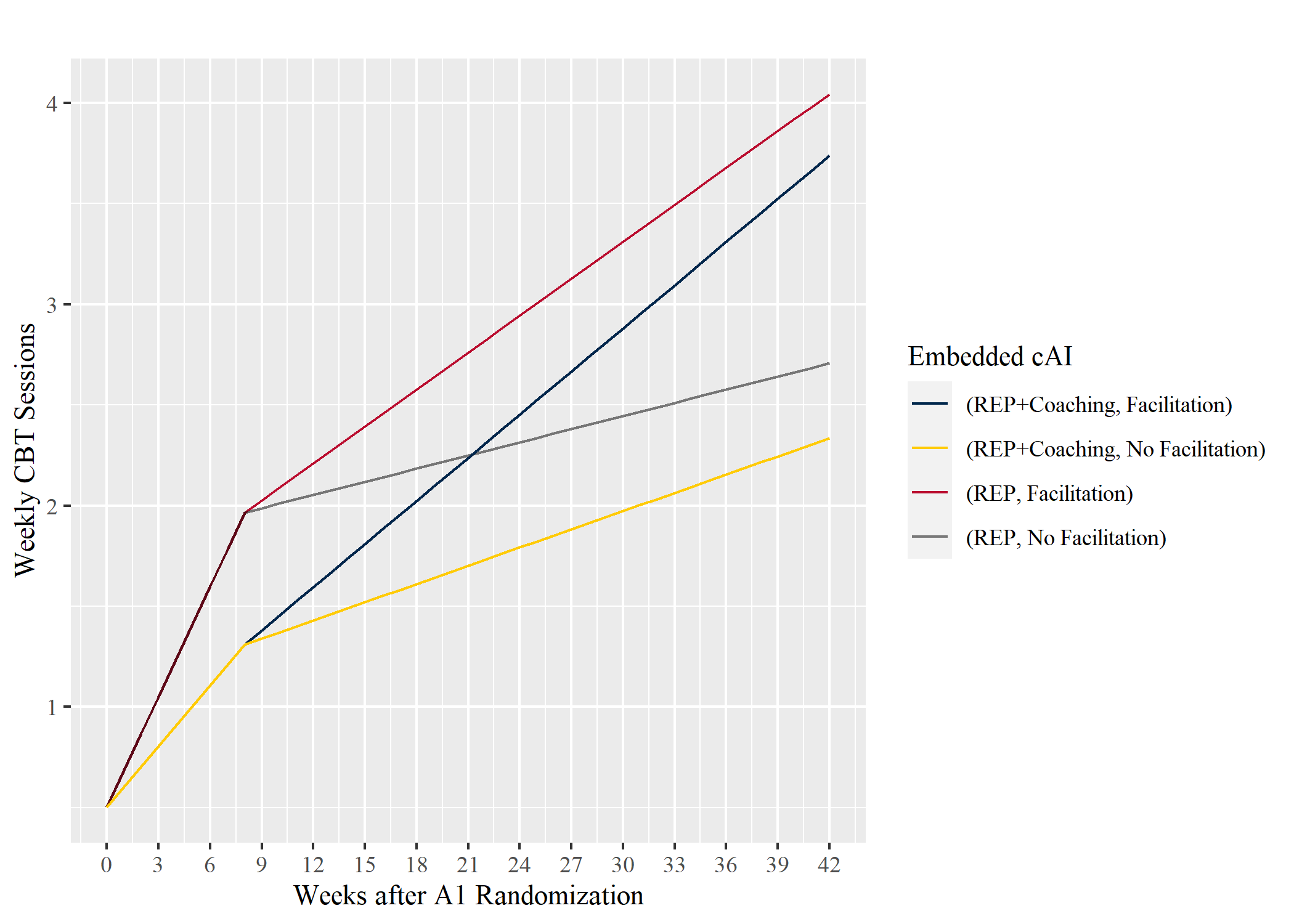
Figure 3: Average Weekly CBT Sessions by Embedded cAI - ASIC

Figure 4 shows the point estimates and $95\%$ confidence intervals for the six pairwise contrasts in embedded cAIs with respect to the ASIC primary outcome. As shown in the figure, none of the embedded cAIs were significantly different from each other in this respect. In particular, we see a near-zero effect in the primary aim comparison. Subsequently, we would fail to reject the null hypothesis that $\mathbb{E}\left[\sum Y_{t}^{(1,1)}\right]=\mathbb{E}\left[\sum Y_{t}^{(-1,-1)}\right]$. This does not suggest a null effect for either embedded cAI; rather, it merely indicates a lack of evidence for a difference in the two. Such information can be useful to decision-makers - if the more intensive (REP+Coaching, Facilitation) cAI does not outperform the less intensive (REP, No Facilitation), then policymakers may wish to employ the more easily-scalable option.

Furthermore, as the primary aim in question is a static end-of-study comparison, we can compare our approach with the existing approach to analyze such aims presented in NeCamp et al. (2017). As shown in Figure 4, both approaches give similar point estimates for the difference in expected total CBT delivery in each of the six pairwise comparisons between embedded cAIs. However, the estimates using the longitudinal approach had $95\%$ confidence intervals that were $\approx 26\%$ narrower, on average, compared with those obtained via the static approach. Section 8.2 further discusses this phenomenon in the case when one models three time points.

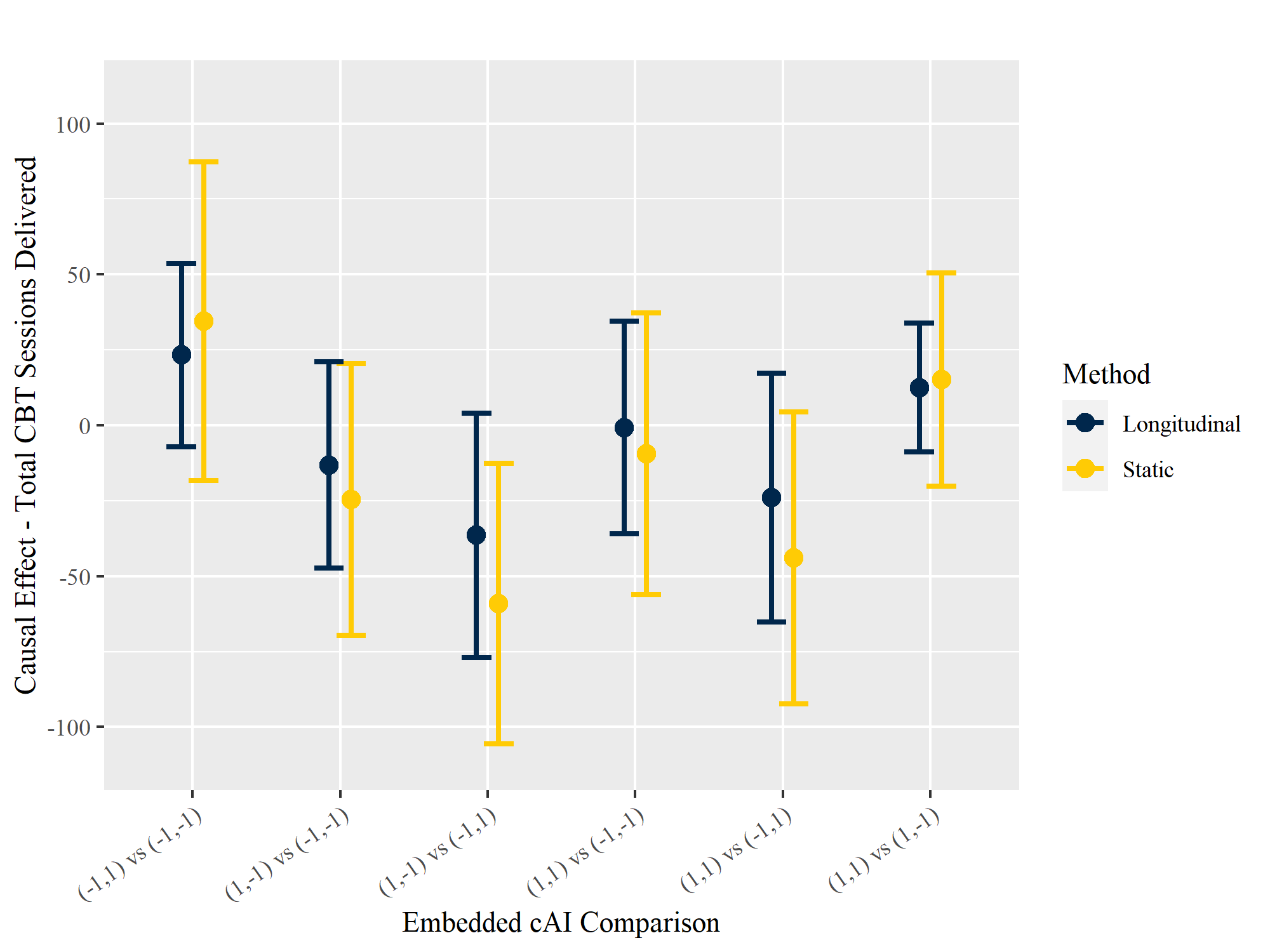
Figure 4: Longitudinal and Static Estimates of Aggregate CBT Delivery Differences by Embedded cAI - ASIC

7.2 Longitudinal Follow-Up Analyses

7.2.1 Second-Stage Slope

Examining Figure 3 presents several insights into the trajectory of CBT delivery that would be masked in an end-of-study analysis. As shown in the figure, after the second decision point, the marginal mean trajectories for CBT delivery for (REP, Facilitation) and (REP+Coaching, Facilitation) both outpace their “No Facilitation” counterparts. This pattern suggests that adding Facilitation for non-responding schools may cause schools to more quickly shed barriers for CBT delivery.

While the methods presented in this manuscript were introduced in the context of primary aim analyses, they are equally applicable to secondary and exploratory aim analyses. In particular, collecting and analyzing repeated measurements of CBT delivery allows us to conduct inference to investigate the impact of Faciliation by comparing second-stage treatment slopes for CBT delivery. Table 5 below shows the results of this comparison for the six pairwise comparisons of the four embedded cAIs in ASIC.

Pairwise cAI Comparison	Estimate	SE	$95\%$ Confidence Interval	p-Value
(1,1) vs (1,-1)	0.041	0.04	(-0.03, 0.12)	0.276
(1,1) vs (-1,1)	0.010	0.04	(-0.08, 0.10)	0.811
(1,1) vs (-1,-1)	0.050	0.04	(-0.03, 0.13)	0.242
(1,-1) vs (-1,1)	-0.031	0.04	(-0.11, 0.05)	0.454
(1,-1) vs (-1,-1)	0.008	0.04	(-0.07, 0.09)	0.829
(-1,1) vs (-1,-1)	0.039	0.03	(-0.03, 0.11)	0.249

Table 5: Comparison of Second Stage Slope for Weekly CBT Delivery - ASIC

7.2.2 Nonlinear Temporal Trend

Given the time between second-stage treatment decision and end-of-study, a trial designer may prefer a marginal mean model that evolves at a rate slower than $t$ (Borghi et al., 2005). For example,

$$\begin{split}\tilde{\mu}_{t}(a_{1},a_{2NR};\theta)&=\gamma_{0}+\eta X_{ij}+\mathbbm{1}_{t\leq t^{*}}\left(\gamma_{1}\sqrt{t}+\gamma_{2}a_{1}\sqrt{t}\right)+\mathbbm{1}_{t>t^{*}}\Bigg{(}\gamma_{1}\sqrt{t^{*}}+\gamma_{2}a_{1}\sqrt{t^{*}}\\ &\hskip 14.22636pt+\left(\gamma_{3}+\gamma_{4}a_{1}+\gamma_{5}a_{2NR}+\gamma_{6}a_{1}a_{2NR}\right)\left(\sqrt{t}-\sqrt{t^{*}}\right)\Bigg{)}.\end{split}$$ (6)

Figure A1 in Appendix A1 shows the marginal mean trajectories under model $\tilde{\mu}$. Furthermore, we revisit the analysis of second-stage slope under this alternate model in Table A2 in Appendix A1. As the figure and table suggest, this approach yielded results that were largely consistent with the original, providing little evidence of meaningful difference.

8 Simulation Study

This section presents three simulation studies to better understand the operating characteristics of the proposed estimator across a variety of settings. Data-generative models were chosen to mimic ASIC, a prototypical clustered SMART, but with three time points: baseline ($t_{0}=0$), end of first stage of intervention ($t^{*}=1$), and end of second stage of intervention ($t_{T}=2$). Without loss of generality, the output from all simulation studies report metrics for the comparison of embedded cAIs $(1,1)$ and $(-1,-1)$ with respect to end-of-study marginal mean estimates. The data-generative models were designed to model real-world data generation from a clustered SMART and allow us to manipulate the $(i)$ true effect size for this comparison, $(ii)$ sample size, $(iii)$ between-person covariance structure, and $(iv)$ within-person covariance structure. Unless otherwise specified, all analyses in the simulation experiments employ the finite-sample adjustments discussed in Pan et al. (2024+). Additional details are provided in Appendix A6.

8.1 Estimator Validity

The purpose of the first simulation experiment was to verify the consistency of the estimator and examine empirical performance in small samples. We hypothesized, as supported by the theoretical results stated in Section 6.2 that in large samples, the estimator would coalesce around the true value. Furthermore, we hypothesized that the estimator would be more volatile in small samples, but generally centered around the true mean.

Table 6 below displays the performance of a correctly-specified estimator on simulated data inspired by weekly CBT session trends in the ASIC data. As shown below, relative bias ($\frac{\left(\hat{\mu}_{2}((1,1))-\hat{\mu}_{2}((-1,-1))\right)-\left(\mu_{2}((1,1))-\mu_{2}((-1,-1))\right)}{\mu_{2}((-1,-1))}$) is negligible across sample sizes and the estimator tightens around the true difference as $N$ grows. Furthermore, we achieve near-nominal coverage when applying the finite-sample adjustments discussed above.

Number of Clusters	Relative Bias	SD	RMSE	Coverage
N=20	-0.040	2.141	2.144	0.903
N=30	-0.028	1.768	1.770	0.908
N=40	-0.009	1.532	1.532	0.921
N=50	-0.017	1.366	1.366	0.927
N=75	-0.014	1.105	1.106	0.938
N=100	-0.004	0.966	0.966	0.942
N=500	0.000	0.429	0.429	0.952

Table 6: Estimator Performance by Sample Size

8.2 Efficiency Comparison with Static Analysis

The purpose of the second simulation experiment was to examine the effect of incorporating repeated measurements on power when estimating differences in mean end-of-study outcomes. With this inquiry in mind, we compared the method presented in this report with the static approach outlined in NeCamp et al. (2017) (which models the outcome only at time $t=2$). We hypothesized that, when within-unit correlation was high, modeling the outcome trajectory would present a more powerful approach than solely modeling the outcome at end-of-study. We further hypothesized that the two approaches would perform similarly in outcomes with lower within-person correlation.

NeCamp’s earlier work on analyses of cSMARTs introduced a sample size formula for comparing embedded cAIs with respect to a single, end-of-study outcome (NeCamp et al., 2017). We intended for this simulation framework to align with the perspective of the primary aim design. Therefore, using this formula, we estimated the minimum sample size required to achieve $80\%$ power for detecting true effect sizes of $0.2$, $0.5$, $0.8$, and $1.0$ using NeCamp’s static approach.

To generate data, we considered two separate approaches, intending to examine high- and low-correlation settings inspired by ASIC data. Both approaches involve an AR(1) correlation structure, homogeneous over embedded cAI ($\rho_{high}\approx 0.58,\text{ }\rho_{low}\approx 0.27$). In Tables 7(a) and 7(b), we do not employ any finite-sample adjustments (as NeCamp’s sample size formula does not incorporate such adjustments).

Effect Size $(N)$	RMSE		Coverage		Power
	Static	Long.	Static	Long.	Static	Long.
$\delta=0.2$ ($n=633$)	0.33	0.33	0.95	0.95	0.81	0.82
$\delta=0.5$ ($n=102$)	0.83	0.82	0.94	0.94	0.82	0.83
$\delta=0.8$ ($n=40$)	1.32	1.32	0.93	0.92	0.83	0.83
$\delta=1.0$ ($n=26$)	1.65	1.65	0.91	0.91	0.84	0.85

(a) Low Correlation

Effect Size $(N)$	RMSE		Coverage		Power
	Static	Long.	Static	Long.	Static	Long.
$\delta=0.2$ ($n=661$)	7.03	6.18	0.95	0.95	0.81	0.90
$\delta=0.5$ ($n=106$)	17.58	15.53	0.94	0.94	0.82	0.90
$\delta=0.8$ ($n=42$)	28.15	24.77	0.93	0.93	0.83	0.91
$\delta=1.0$ ($n=27$)	35.04	30.74	0.91	0.92	0.85	0.92

(b) High Correlation

Table 7: Static vs Longitudinal Power Comparison

Table 7(b) shows material power gains for the longitudinal estimator over the static estimator. In this “high correlation” setting, outcomes at times $t=0,1$ to provide more information about outcomes at time $t=2$ than in the less-correlated setting. Similarly, the longitudinal estimator sees material improvement over its static counterpart in terms of RMSE in this environment as well.

While a longitudinal approach outperforms a static approach in a highly-correlated data-generative setting, the two approaches perform similarly in a low-correlation setting. Therefore, Tables 7(a) and 7(b) suggest that, when repeated measures of an outcome are available, an analyst will not sacrifice statistical performance by modeling the outcome longitudinally.

We end this discussion by noting two important caveats to the results in Table 7(b). First, the efficiency gains highlighted in this table are not due to modeling assumptions on the temporal trajectory of the outcome $Y$. In this simulation study, we employed marginal model 4, which is fully saturated when modeling only $Y_{t_{0}}$, $Y_{t^{*}}$, and $Y_{t_{T}}$. This suggests that analysts can incorporate repeated measurements in end-of-study outcome comparisons to potentially achieve material precision gains without employing stringent modeling assumptions. It is likely the case that including more time points in an analysis can cause further precision gains, although it may expose the analyst to marginal mean model misspecification (as incorporating additional outcomes measurement would highlight Equation 4’s assumption of linear trends between times $t_{0}$ and $t^{*}$, as well as $t^{*}$ and $t_{T}$). Second, this pattern may cause a trial designer to reject NeCamp’s sample size calculator in the hopes that incorporating repeated measurements can increase power. While these analyses suggest that one would not lose power by incorporating repeated measurements, one is not guaranteed to see material power gain. Given the static/longitudinal power alignment in Table 7(a), we recommend the use of NeCamp’s sample size formula to power a study even when repeated measurements are to be available, following a conservative approach to ensure adequate power under varying conditions.

8.3 Working Variance Modeling

Modeling longitudinal outcomes in clustered SMARTs requires careful specification of the working variance, as variance modeling plays a central role in both estimation and inference. A primary contribution of this paper is the development of methods that account for these variance structures, making it essential to assess how different working variance choices influence key performance metrics. The purpose of the third simulation experiment was to examine the impacts of working variance modeling choices on estimator performance. We hypothesized that correctly specifying the marginal variance structure would show material efficiency gains, but little improvement in coverage (given the asymptotic normality of the estimator under working variance misspecification, as discussed in Section 6.2).

Figure 5 shows the comparative performance of estimators with various working variance models. As discussed in Appendix A6.4 of Supplement 2, this comparison is based on a data-generative model with complex correlation and heteroscedastic variance.

Figure 5(a) shows that choice of working variance structure does not heavily impact coverage rate. This is in line with the results in Section 6.2, as the asymptotic normality of the estimator holds under working variance misspecification. While these results suggest choice of working variance estimate will not affect the validity of parameter estimates/confidence intervals, Figure 5(b) suggests these choices can impact estimator efficiency. For a given working variance model ($wv$), this plot shows $\overline{\left(SE_{wv}/SE_{iid}\right)}$ (i.e., the average ratio of the standard error obtained under $wv$ and that obtained under a homoscedastic-independent working variance model) across sample sizes. As $N$ grows, the correctly specified working variance model, represented by the dashed purple line, outperforms its counterparts. For large $N$, it achieves a $\approx 10\%$ efficiency gain over the IID approach. Additionally, heteroscedastic working variance models tend to outperform those with temporally homogeneous variance.

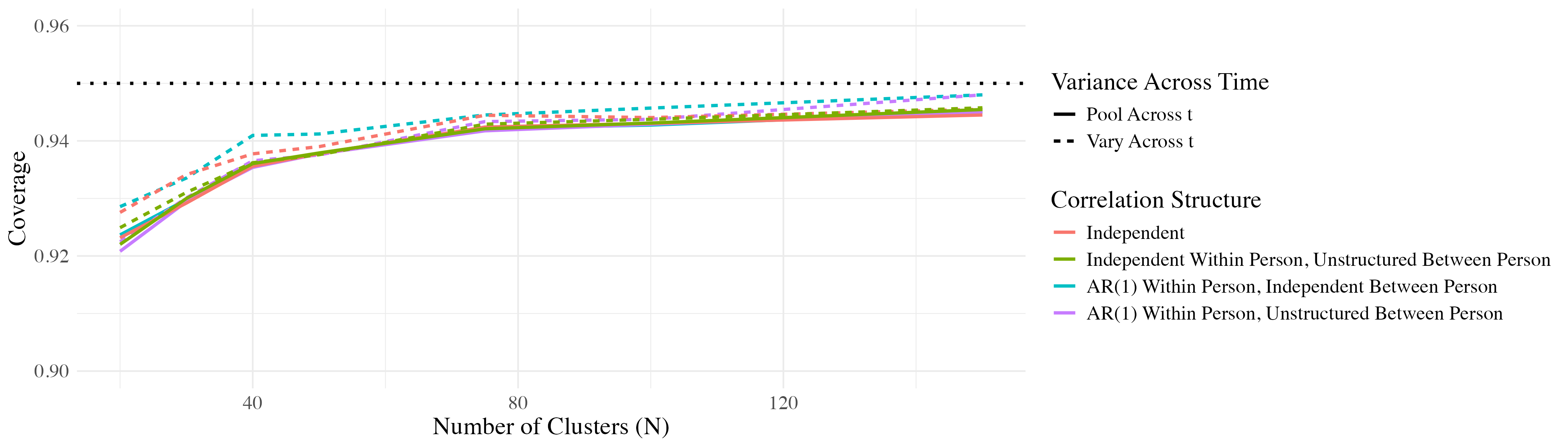
(a) Coverage Rates

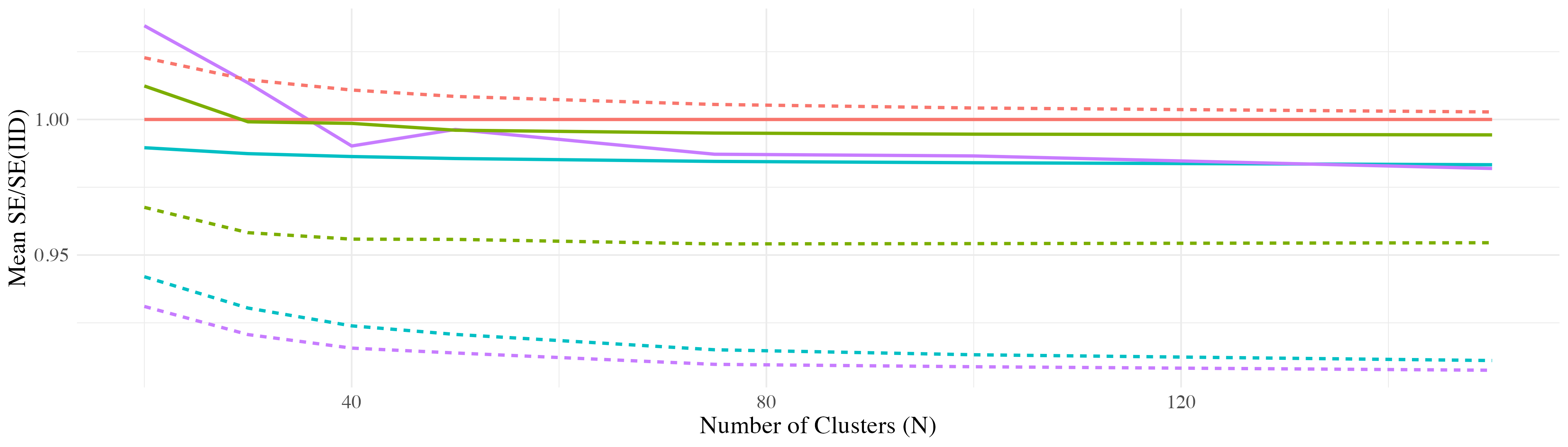
(b) Relative Efficiency (Homoscedastic-Independent Baseline)

Figure 5: Performance of Different Working Variance Models Across Sample Sizes

As a follow-up to this analysis, we investigated the efficiency trade-offs associated with employing complex working variance models when the true data-generating variance structure is simple (i.e., homoscedastic and independent). Figure A2 in Appendix A1 presents the corresponding results in this scenario. The figure demonstrates that in such settings, the choice of working variance model has minimal impact on efficiency. These findings suggest that the risks associated with under-specifying the working variance structure may outweigh the potential inefficiencies introduced by over-specification.

9 Discussion

The sections above detail a novel approach for analyzing longitudinal data arising from clustered SMARTs. This method equips domain scientists with a tool to explore temporal patterns in outcomes in their cSMART analyses. In the context of designing adaptive interventions, understanding the trajectory of improvement in a target outcome is often crucial. While end-of-study analyses in cSMARTs can provide valuable insights, they may overlook important temporal dynamics that could inform the optimization of adaptation strategies in a cAI (Nahum-Shani et al., 2020). For example, as observed in ASIC, mapping the trend in expected weekly CBT delivery by embedded cAI suggested that protocols which incorporated Facilitation for struggling schools led to faster rates of CBT delivery growth compared with protocols which did not. As discussed in Section 7, we can use the proposed method to conduct formal inference with respect to such comparisons. Additionally, Section 7 and the power analysis in Section 8.2 demonstrated that incorporating repeated outcome measurements can yield more precise estimates of traditional end-of-study objectives compared to existing methods that rely solely on the final outcome.

Following the introduction of methods for analyzing repeated measures in individually-randomized SMARTs, researchers have been able to address a wider range of substantive questions regarding temporal treatment effects. These more detailed SMART analyses hold significant promise for the design of adaptive interventions, offering researchers deeper insight to inform adaptive intervention development (Nahum-Shani et al., 2020). Similarly, exploring such questions in clustered settings can give domain scientists the tools to construct more effective clustered adaptive interventions.

Supplementary Material

A1 Additional Figures and Tables

Embedded cAI	$\rho_{w}$ (AR(1) Structure)	$\rho_{b}$ (Exchangeable Structure)
(REP+Coaching, Facilitation)	0.09	0.14
(REP+Coaching, No Facilitation)	0.44	0.05
(REP, Facilitation)	0.30	0.03
(REP, No Facilitation)	0.33	0.23

Table A1: Marginal Correlation Estimates - ASIC

Comparison	Estimate	SE	CI	p-Value
(1,1) vs (1,-1)	0.04	0.04	(-0.04, 0.11)	0.317
(1,1) vs (-1,1)	0.01	0.04	(-0.07, 0.09)	0.817
(1,1) vs (-1,-1)	0.05	0.04	(-0.04, 0.13)	0.262
(1,-1) vs (-1,1)	-0.03	0.04	(-0.11, 0.05)	0.490
(1,-1) vs (-1,-1)	0.01	0.04	(-0.07, 0.09)	0.834
(-1,1) vs (-1,-1)	0.04	0.03	(-0.03, 0.10)	0.283

Table A2: ASIC: Second-Stage Slope Comparison for Alternate Marginal Model

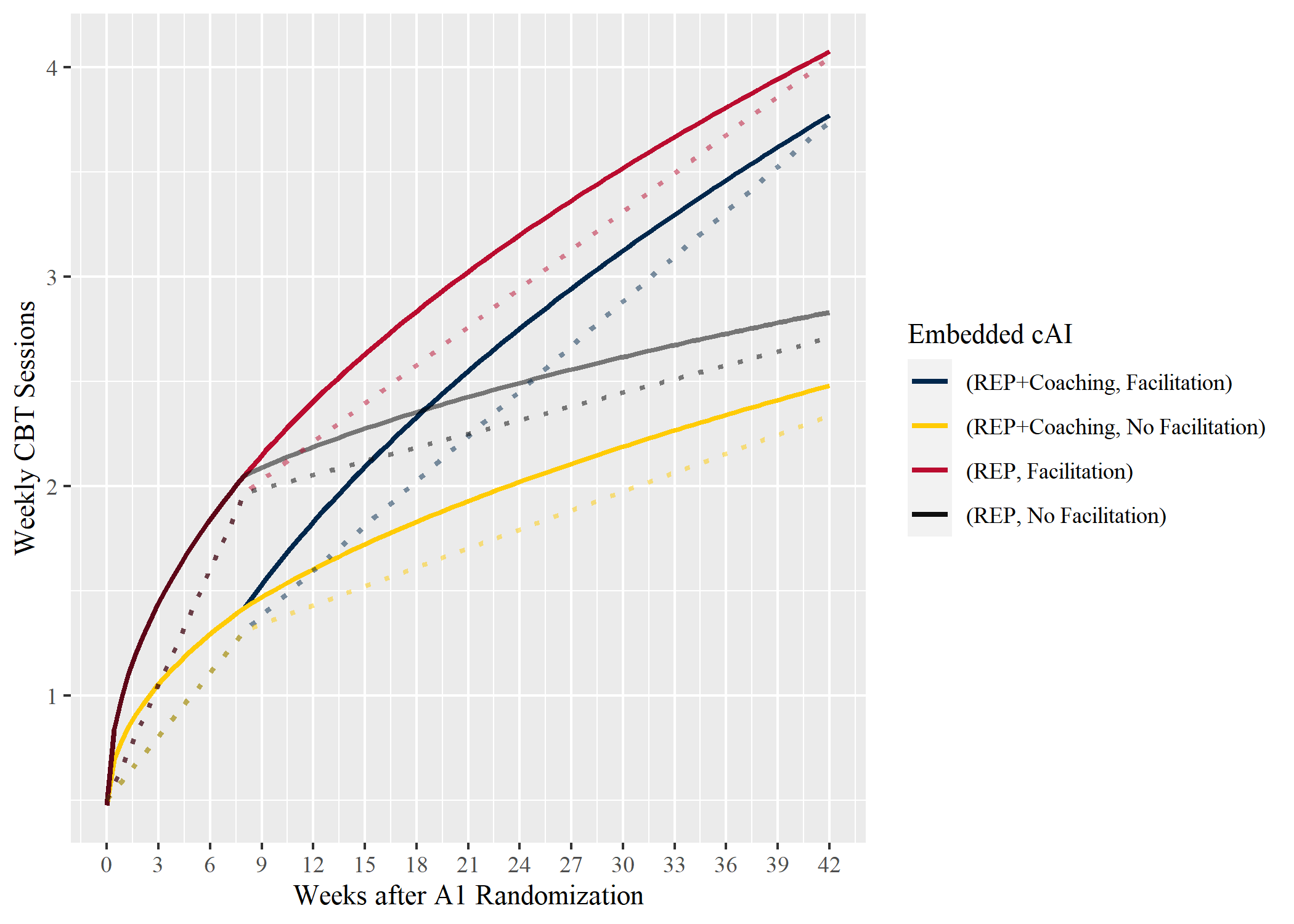
Figure A1: ASIC Trajectories under Alternate Marginal Mean Model

Dotted lines represent linear trajectories under $\mu$.

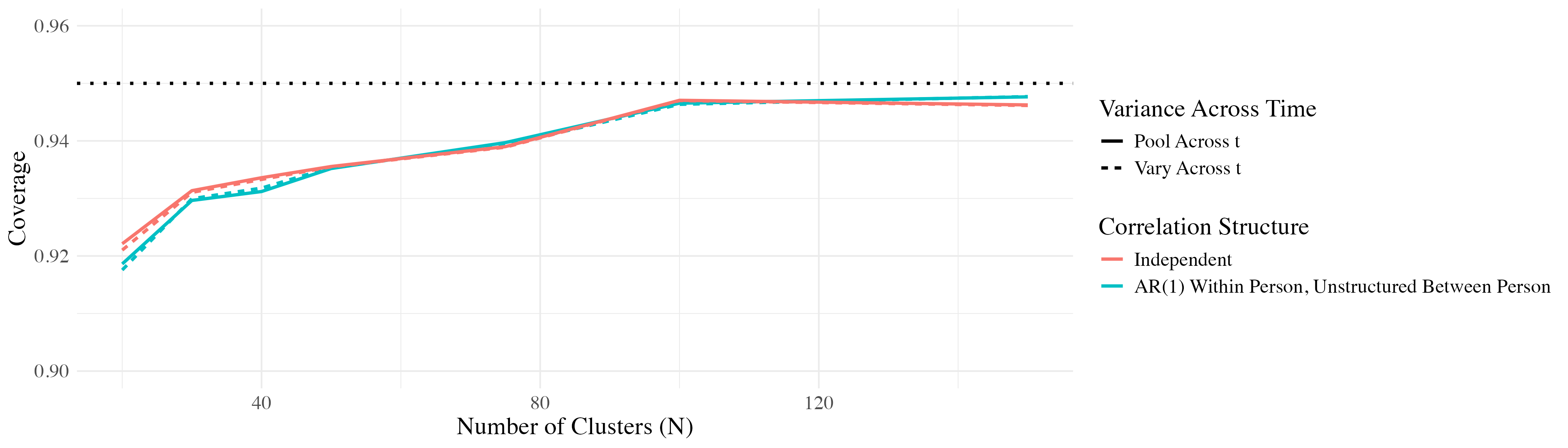
(a) Coverage Rates

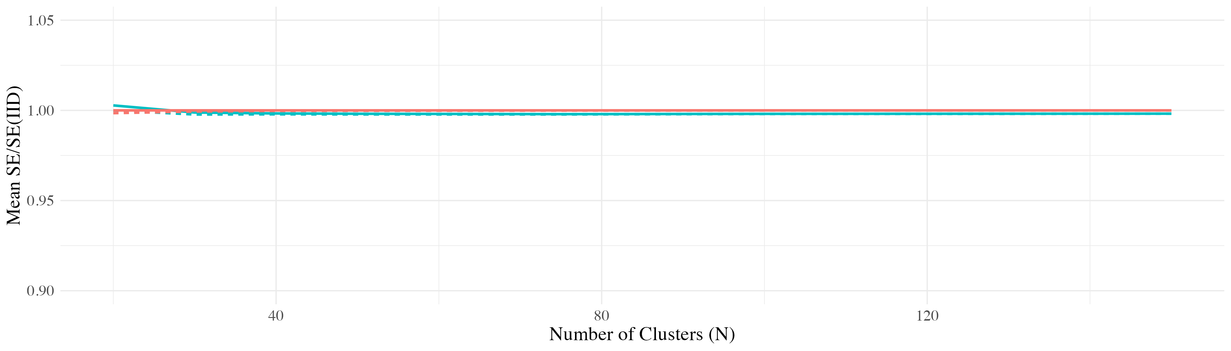
(b) Relative Efficiency (IID Baseline)

Figure A2: Performance of Different Working Variance Models Across Sample Sizes - Homoscedastic-Independent Data Generative Model

A2 Further Discussion of Working Variance

As discussed in Section 5.2 of the main body, we let $V^{d}\left(\mathbf{X};\alpha\right)$ denote our working variance model; parameterized by $\alpha=\begin{bmatrix}\sigma\\ \rho\end{bmatrix}$, where $V_{i}^{d}\left(\mathbf{X}_{i};\alpha\right)$ takes the general form

$$V^{d}\left(\mathbf{X}_{i};\alpha\right)=\mathbf{S}_{i}^{d}(\sigma)^{\frac{1}{2}}\boldsymbol{\mathrm{P}}_{i}^{d}(\rho)\mathbf{S}_{i}^{d}(\sigma)^{\frac{1}{2}}.$$

Here, the $n_{i}(T+1)\times n_{i}(T+1)$ matrices $\mathbf{S}_{i}^{d}(\sigma)$ and $\boldsymbol{\mathrm{P}}_{i}^{d}(\rho)$ correspond to variance and correlation matrices (respectively), and have the broad structures described below.

$$\mathbf{S}_{i}^{d}(\sigma)=\begin{bmatrix}S^{d}(\sigma)&&0\\ &\ddots&\\ 0&&S^{d}(\sigma)\\ \end{bmatrix}\text{, }\boldsymbol{\mathrm{P}}_{i}^{d}(\rho)=\begin{bmatrix}W^{d}(\rho)&B^{d}(\rho)&\dots&B^{d}(\rho)\\ B^{d}(\rho)&W^{d}(\rho)&&\\ \vdots&&\ddots&\\ B^{d}(\rho)&&&W^{d}(\rho)\\ \end{bmatrix},$$

where $S^{d}(\sigma)$ is a $(T+1)\times(T+1)$ diagonal matrix with entries corresponding to $\mathbb{V}\left[Y_{t_{0}}{{}^{(d)}}\mid\mathbf{X}\right],\ldots,\mathbb{V}\left[Y_{t_{T}}{{}^{(d)}}\mid\mathbf{X}\right]$ and $W^{d}(\rho)$ and $B^{d}(\rho)$ are within and between person $(T+1)\times(T+1)$ correlation matrices representing $corr\left(Y{{}^{(d)}}_{i,j,.},Y{{}^{(d)}}_{i,j,.}\mid\mathbf{X}\right)$ and $corr\left(Y{{}^{(d)}}_{i,j,.},Y{{}^{(d)}}_{i,j^{\prime},.}\mid\mathbf{X}\right)$ (respectively).

The exact forms of $S^{d}(\sigma)$, $W^{d}(\rho)$, $B^{d}(\rho)$ depend on the variance structure the analyst chooses to model. Using our illustrative model from Section 5.2 of the main body, we can consider a working variance model that is exchangeable within-person and between-person. Furthermore, we will assume heterogeneous variance across time and adaptive intervention. This choice of variance structure induces the following forms of $S^{d}(\sigma)$, $W^{d}(\rho)$, and $B^{d}(\rho)$

$$S^{d}(\sigma)=\begin{bmatrix}\left(\sigma^{d}_{t_{0}}\right)^{2}&&0\\ &\ddots&\\ 0&&\left(\sigma^{d}_{t_{T}}\right)^{2}\end{bmatrix},\hskip 7.11317ptW^{d}(\rho)=\begin{bmatrix}1&&\rho^{d}_{w}\\ &\ddots&\\ \rho^{d}_{w}&&1\end{bmatrix},\text{ and}\hskip 7.11317ptB^{d}(\rho)=\begin{bmatrix}\rho^{d}_{b}&&\rho^{d}_{b}\\ &\ddots&\\ \rho^{d}_{b}&&\rho^{d}_{b}\end{bmatrix},$$

where $\sigma=\begin{bmatrix}\sigma^{d_{1}}_{t_{0}}&\sigma^{d_{1}}_{t_{1}}&\dots&\sigma^{d_{1}}_{t_{T}}&\sigma^{d_{2}}_{t_{0}}&\dots&\dots&\sigma^{d_{D}}_{t_{T}}\end{bmatrix}^{T},$ and $\rho=\begin{bmatrix}\rho^{d_{1}}_{w}&\rho^{d_{1}}_{b}&\rho^{d_{2}}_{w}&\rho^{d_{2}}_{b}&\dots&\rho^{d_{D}}_{w}&\rho^{d_{D}}_{b}\end{bmatrix}^{T}$.

A3 Variance Estimation

Section 6 of the main body discusses how to construct variance estimates under an example working variance for each step in the model fitting procedure presented in the main body of the report. This appendix discusses how to adapt this algorithm for alternative working variance structures.

Recall the general form of the working variance, discussed in detail in Appendix A2:

$$V^{d}\left(\mathbf{X}_{i};\alpha\right)=\mathbf{S}_{i}^{d}(\sigma)^{\frac{1}{2}}\boldsymbol{\mathrm{P}}_{i}^{d}(\rho)\mathbf{S}_{i}^{d}(\sigma)^{\frac{1}{2}}.$$

This appendix concerns the estimation of the $\alpha$ parameters which define $V^{d}\left(\mathbf{X}_{i};\alpha\right)$. In the case of repeated measures in clustered SMARTs, this involves three steps: Estimation of the marginal variance components, estimation of the within-person correlation components, and estimation of the between-person correlation components.

Recall from Section 6 of the main body that variance estimation at each step ($s$) in the iterative model fitting algorithm relies on the model residuals from the previous step: $\hat{\varepsilon}^{d,s}_{i}=\mathbf{Y}_{i}-\boldsymbol{\mu}(d,\mathbf{X}_{i};\hat{\theta}_{s-1})$.

A3.1 Marginal Variance Components

We first seek an estimate of $\mathbb{V}\left[Y_{i,j,t}{{}^{(d)}}\mid\mathbf{X}\right]$. We consider two separate modeling decisions:

1. $S^{d}(\sigma)=\begin{bmatrix}\left(\sigma^{d}_{t_{0}}\right)^{2}&&0\\ &\ddots&\\ 0&&\left(\sigma^{d}_{t_{T}}\right)^{2}\end{bmatrix}$, and

2. $S^{d}(\sigma)=\begin{bmatrix}\left(\sigma_{t_{0}}\right)^{2}&&0\\ &\ddots&\\ 0&&\left(\sigma_{t_{T}}\right)^{2}\end{bmatrix}.$

The first case describes a working variance model in which the marginal variances can differ across embedded AI, whereas the second describes a marginal variance model that is homogeneous with respect to embedded AI. Table A3 below presents estimators for these quantities.

Marginal Variance Structure	$\mathbb{V}\left[Y_{i,j,t}{{}^{(d)}}\mid\mathbf{X}\right]$	Estimator
Heterogeneous with respect to embedded cAI	$\left(\sigma_{t}^{d}\right)^{2}$	$\left(\hat{\sigma}^{d}_{t}\right)^{2}=\frac{\displaystyle\displaystyle\sum_{i=1}^{N}I_{i}(d)W_{i}\displaystyle\sum_{j=1}^{n_{i}}\left(\hat{\varepsilon}^{d,s}_{i,j,t}\right)^{2}}{\displaystyle\displaystyle\sum_{i=1}^{N}W_{i}I_{i}(d)n_{i}}$
Homogeneous with respect to embedded cAI	$\sigma_{t}^{2}$	$\left(\hat{\sigma}_{t}\right)^{2}=\frac{\displaystyle\displaystyle\sum_{i=1}^{N}\displaystyle\sum_{d\in\mathcal{D}}I_{i}(d)W_{i}\displaystyle\sum_{j=1}^{n_{i}}\left(\hat{\varepsilon}^{d,s}_{i,j,t}\right)^{2}}{\displaystyle\displaystyle\sum_{i=1}^{N}\displaystyle\sum_{d\in\mathcal{D}}I_{i}(d)W_{i}n_{i}}$

Table A3: Marginal Variance Estimators

In addition to pooling over embedded AIs, a researcher could also pool over time, taking either

$$\left(\hat{\sigma}^{d}\right)^{2}=\frac{1}{T}\sum_{k=0}^{T}\left(\hat{\sigma}^{d}_{t_{k}}\right)^{2}\text{ or }\left(\hat{\sigma}\right)^{2}=\frac{1}{T}\sum_{k=0}^{T}\left(\hat{\sigma}_{t_{k}}\right)^{2},$$

depending on whether they wanted to pool over embedded cAI as well (where $\hat{\sigma}_{t}$ and $\hat{\sigma}_{t}^{d}$ are as obtained above).

A3.2 Within-Person Correlation

After obtaining marginal variance estimates, we must estimate within-person correlation components. This corresponds to estimating the $(T+1)\times(T+1)$ diagonal blocks of $\boldsymbol{\mathrm{P}}_{i}$.

We will consider four different structures for these blocks. Here, we present estimators that are heterogeneous with respect to embedded AI; however, one could homogenize over adaptive interventions just as in Table A3. We note that, while an analyst may wish to pool across time and/or embedded cAI to estimate marginal variance components, the $\hat{\sigma}^{d}_{t_{l}}$ terms in Tables A4 and A5 should not be not be pooled over time or embedded cAI to ensure stable correlation estimates.

Within-Person Correlation Structure	$\text{Corr}\left(Y_{i,j,t_{l}}{{}^{(d)}},Y_{i,j,t_{m}}{{}^{(d)}}\right)$	Estimator
AR(I)	$\begin{cases}1&\text{ if $t_{l}=t_{m}$}\\ \left(\rho_{w}^{d}\right)^{|l-m|}&\text{ otherwise}\end{cases}$	$\hat{\rho}^{d}_{w,AR(I)}=\frac{\displaystyle\displaystyle\sum_{i=1}^{N}I_{i}(d)W_{i}\displaystyle\sum_{j=1}^{n_{i}}\displaystyle\sum_{l=0}^{T-1}\left(\frac{\hat{\varepsilon}^{d,s}_{i,j,t_{l}}}{\hat{\sigma}^{d}_{t_{l}}}\right)\left(\frac{\hat{\varepsilon}^{d,s}_{i,j,t_{l+1}}}{\hat{\sigma}^{d}_{t_{l+1}}}\right)}{\displaystyle\displaystyle\sum_{i=1}^{N}I_{i}(d)W_{i}n_{i}T}$
Exchangeable	$\begin{cases}1&\text{ if }t_{l}=t_{m}\\ \rho_{w}^{d}&\text{ otherwise}\end{cases}$	$\hat{\rho}^{d}_{w,Ex}=\frac{\displaystyle\displaystyle\sum_{i=1}^{N}I_{i}(d)W_{i}\displaystyle\sum_{j=1}^{n_{i}}\displaystyle\sum_{l=0}^{T}\displaystyle\sum_{\begin{subarray}{c}m=0\\ m\neq l\end{subarray}}^{T}\left(\frac{\hat{\varepsilon}^{d,s}_{i,j,t_{l}}}{\hat{\sigma}^{d}_{t_{l}}}\right)\left(\frac{\hat{\varepsilon}^{d,s}_{i,j,t_{m}}}{\hat{\sigma}^{d}_{t_{m}}}\right)}{\displaystyle\displaystyle\sum_{i=1}^{N}I_{i}(d)W_{i}n_{i}(T+1)T}$
Unstructured	$\begin{cases}1&\text{ if }t_{l}=t_{m}\\ \rho^{d}_{w,t_{l},t_{m}}&\text{ otherwise}\end{cases}$	$\hat{\rho}^{d}_{w,Un,t_{l},t_{m}}=\frac{\displaystyle\displaystyle\sum_{i=1}^{N}I_{i}(d)W_{i}\displaystyle\sum_{j=1}^{n_{i}}\left(\frac{\hat{\varepsilon}^{d,s}_{i,j,t_{l}}}{\hat{\sigma}^{d}_{t_{l}}}\right)\left(\frac{\hat{\varepsilon}^{d,s}_{i,j,t_{m}}}{\hat{\sigma}^{d}_{t_{m}}}\right)}{\displaystyle\displaystyle\sum_{i=1}^{N}I_{i}(d)W_{i}n_{i}}$
Independent	$\begin{cases}1&\text{ if }t_{l}=t_{m}\\ 0&\text{ otherwise}\end{cases}$	$\hat{\rho}^{d}_{w,In}=0$

Table A4: Within-Person Correlation Estimators

A3.3 Between-Person Correlation

Finally, we must estimate within-cluster between person correlation components. This corresponds to estimating the $(T+1)\times(T+1)$ off-diagonal blocks of $\boldsymbol{\mathrm{P}}_{i}$.

We consider three different structures for these blocks. As before, we present estimators that are heterogeneous with respect to embedded AI; however, one could homogenize over adaptive interventions just as in Table A3.

Between-Person Correlation Structure	$\text{Corr}\left(Y_{i,j,t_{l}}{{}^{(d)}},Y_{i,k,t_{m}}{{}^{(d)}}\right)$ $\left(j\neq k\right)$	Estimator
Exchangeable	$\rho_{b}^{d}$	$\hat{\rho}^{d}_{b,Ex}=\frac{\displaystyle\displaystyle\sum_{i=1}^{N}I_{i}(d)W_{i}\displaystyle\sum_{j=1}^{n_{i}}\displaystyle\sum_{\begin{subarray}{c}k=1\\ k\neq j\end{subarray}}^{n_{i}}\displaystyle\sum_{l=0}^{T}\displaystyle\sum_{m=0}^{T}\left(\frac{\hat{\varepsilon}^{d,s}_{i,j,t_{l}}}{\hat{\sigma}^{d}_{t_{l}}}\right)\left(\frac{\hat{\varepsilon}^{d,s}_{i,k,t_{m}}}{\hat{\sigma}^{d}_{t_{m}}}\right)}{\displaystyle\displaystyle\sum_{i=1}^{N}I_{i}(d)W_{i}n_{i}\left(n_{i}-1\right)(T+1)^{2}}$
Unstructured	$\rho^{d}_{b,t_{l},t_{m}}$	$\hat{\rho}^{d}_{b,Un,t_{l},t_{m}}=\frac{\displaystyle\displaystyle\sum_{i=1}^{N}I_{i}(d)W_{i}\displaystyle\sum_{j=1}^{n_{i}}\displaystyle\sum_{\begin{subarray}{c}k=1\\ k\neq j\end{subarray}}^{n_{i}}\left(\frac{\hat{\varepsilon}^{d,s}_{i,j,t_{l}}}{\hat{\sigma}^{d}_{t_{l}}}\right)\left(\frac{\hat{\varepsilon}^{d,s}_{i,k,t_{m}}}{\hat{\sigma}^{d}_{t_{m}}}\right)}{\displaystyle\displaystyle\sum_{i=1}^{N}I_{i}(d)W_{i}n_{i}\left(n_{i}-1\right)}$
Independent	0	$\hat{\rho}^{d}_{b,In}=0$

Table A5: Between-Person Correlation Estimators

A4 Weight Estimation

Analysts often use the known randomization probabilities to construct weights $W_{i}$, as discussed in Section 6 of the main body. The randomized nature of SMARTs ensure that these known-probability weights produce consistent estimates. However, an analyst may choose to estimate the randomization probabilities to gain statistical efficiency. This appendix concerns details regarding weight estimation for the analyst seeking additional efficiency gains.

For an analyst wishing to construct weights to adjust for imbalances in select baseline information, $\mathbf{X}^{w}$, and outcome/covariate information collected between $t_{0}$ and $t^{*}$, $\mathbf{S}^{w}_{1}$, weights for prototypical SMARTs take the form

$$W_{i}=W(\mathbf{x}^{w}_{i},a_{1,i},\mathbf{s}^{w}_{1,i},r_{i},a_{2NR,i})=\dfrac{1}{\mathbb{P}\left[A_{1}=a_{1,i}\mid\mathbf{X}^{w}=\mathbf{x}^{w}_{i}\right]\mathbb{P}\left[A_{2}=a_{2,i}\mid\mathbf{X}^{w}=\mathbf{x}^{w}_{i},A_{1,i}={a_{1,i}},\mathbf{S}^{w}_{1}=\mathbf{s}^{w}_{1,i},R_{i}=r_{i}\right]}.$$

This approach requires estimating $p_{1}\left(a_{1},\mathbf{x}^{w};\hat{\pi}\right)=\hat{\mathbb{P}}\left[A_{1}=a_{1}\mid\mathbf{X}^{w}=\mathbf{x}^{w}\right]$ and $p_{2}\left(a_{1},r,a_{2},\mathbf{x}^{w},\mathbf{s}^{w}_{1};\hat{\pi}\right)=\hat{\mathbb{P}}\left[A_{2}=a_{2}\mid\mathbf{X}^{w}=\mathbf{x}^{w},A_{1}=a_{1},\mathbf{S}^{w}_{1}=\mathbf{s}^{w}_{1},R=r\right]$ for each $a_{1}$, $r$, and $a_{2}$. The estimated weights then have the form

$$\hat{W}_{i}=W(\mathbf{X}^{w}_{i},a_{1,i},\mathbf{s}^{w}_{1,i},r_{i},a_{2,i};\hat{\pi})=\dfrac{1}{p_{1}\left(a_{1,i},\mathbf{x}^{w}_{i};\hat{\pi}\right)p_{2}\left(a_{1,i},r_{i},a_{2,i},\mathbf{x}^{w}_{i},\mathbf{s}^{w}_{1,i};\hat{\pi}\right)}.$$

As we show in Appendix A8, using estimated weights induces the following asymptotic behavior of the estimator:

$$\sqrt{N}\left(\hat{\theta}-\theta_{0}\right)\xrightarrow[N\to\infty]{\mathcal{L}}\mathcal{N}\left(0,\text{ }J^{-1}QJ^{-1}\right),$$

where

$$J =\mathbb{E}\left[\displaystyle\sum_{d\in\mathcal{D}}I(d)W(\pi_{0})D(d,\mathbf{X};\theta)^{T}\Sigma^{d}(\alpha_{+})^{-1}D(d,\mathbf{X};\theta)\right],$$

$$Q =\mathbb{E}\left[UU^{T}\right]-\mathbb{E}\left[US_{\pi_{0}}^{T}\right]\mathbb{E}\left[S_{\pi_{0}}S_{\pi_{0}}^{T}\right]^{-1}\mathbb{E}\left[S_{\pi_{0}}U^{T}\right].$$

A5 Causal Identifiability Assumptions

This section discusses standard assumptions needed to identify the causal effects discussed in the main body of this report. Given the focus of the report, we provide the formal definitions for the assumptions specifically in the prototypical SMART setting and discuss these assumptions more generally in Appendix A7.5.

1. Positivity

   $\mathbb{P}\left[A_{1}=1\right]\in(0,1)$ and $\mathbb{P}\left[A_{2}=1\mid A_{1},R=0\right]\in(0,1)$. I.e., all valid treatment pathways in the SMART have non-zero probability.

2. Consistency

   We consider consistency with respect to response and outcome:

   1. $R_{i}=\mathbbm{1}_{A_{1,i}=1}R_{i}^{(A_{1}=1)}+\mathbbm{1}_{A_{1,i}=-1}R_{i}^{(A_{1}=-1)}$.

   2. $Y_{i,.,t}^{(a_{1},a_{2NR})}=\begin{cases}Y_{i,.,t}&\text{ if $t=t_{0}$}\\ Y_{i,.,t}&\text{ if $a_{1,i}=a_{1}$ and $t\in(t_{0},t^{*}]$}\\ Y_{i,.,t}&\text{ if $a_{1,i}=a_{1}$, $t\in(t^{*},T]$ and either $a_{2NR,i}=a_{2NR}$ or $R_{i}=1$.}\\ \end{cases}$

   We note that the latter consistency equality simply asserts that if, at time $t$, Cluster $i$’s observed treatment history is consistent with a DTR $d$, then $Y_{i,.,t}=Y_{i,.,t}{{}^{(d)}}$. As in Chakraborty and Murphy [2014], we note that this assumption subsumes Rubin’s traditional SUTVA assumption [Rubin, 1980].

3. Sequential (Conditional) Exchangeability

   Given any set of baseline covariates $\mathbf{X}$ (where $\mathbf{X}$ could be empty), and any $(a_{1},a_{2NR})\in\mathcal{D}$, we have

   1. $\left\{\mathbf{Y}_{i}^{(a_{1},a_{2NR})},R_{i}^{(a_{1})}\right\}\perp\!\!\!\perp A_{1}\big{|}_{\mathbf{X}}$.

   2. $\mathbf{Y}_{i}^{(a_{1},a_{2NR})}\perp\!\!\!\perp A_{2}\big{|}_{A_{1,i}=a_{1},R_{i}^{(a_{1})},\mathbf{X}}$.

   I.e., we have both marginal sequential exchangeability and sequential exchangeability conditional on any set of baseline covariates.

A6 Simulation Study Design

In designing the simulation study for this report, we sought to simulate outcomes sequentially, believing this to be more realistic than other data-generative approaches. Simulating outcomes conditional on past outcomes (and response status) necessitated specifying the conditional distribution of the outcomes. Given that our proposed approach fundamentally concerns marginal parameter estimation, we sought to construct a data-generative mechanism consistent with the marginal structural model discussed in Section 5 of the main body. In an attempt to limit the complexity of the simulation model, we limited our simulations to the case of three time points ($t=0,1,2$), where response is determined at time $t^{*}=1$.

Unlike the main body, in this appendix we use $Y_{0}$, $Y_{1}$, and $Y_{2}$ to denote the vector of outcomes for a given cluster at times $t=0,1,2$, respectively. E.g., $Y_{i,t}=\begin{bmatrix}Y_{i,1,t},&\dots&Y_{i,n_{i},t}\end{bmatrix}^{T}$. We use this notation for improved clarity, given the conditional data-generative model described in this appendix.

Implementation code for this data-generative model can be found at https://github.com/GabrielDurham/three_lvl_cSMART_sim_study.

A6.1 Target Structural Mean Model

As discussed above, we sought a conditional data-generative framework; however, as discussed Section 5 of the main body, we propose a marginal modeling framework. Consequently, studying the properties of our estimator requires proper control over the marginal distribution of the generated data.

In the section below, we seek to generate data that mimics the marginal mean model for a prototypical SMART proposed in Section 5 of the main body:

$$\mathbb{E}\left[Y_{i,t}^{(a_{1},a_{2NR})}\mid\mathbf{X}_{i}\right] =\eta\mathbf{X}_{i}+\gamma^{M}_{0}\mathbf{1}_{n_{i}}+\mathbbm{1}_{t\leq 1}\left(\gamma^{M}_{1}t+\gamma^{M}_{2}a_{1}t\right)\mathbf{1}_{n_{i}}$$

$$+\mathbbm{1}_{t>1}\left(\gamma^{M}_{1}+\gamma^{M}_{2}a_{1}+\gamma^{M}_{3}\left(t-1\right)+\gamma^{M}_{4}\left(t-1\right)a_{1}+\gamma^{M}_{5}\left(t-1\right)a_{2NR}+\gamma^{M}_{6}\left(t-1\right)a_{1}a_{2NR}\right)\mathbf{1}_{n_{i}},$$

where we employ the superscript $M$ to denote marginal parameters. We note that the model above is fully saturated in that it allows the specification of all potential expectations: $\mathbb{E}\left[Y^{(.,.)}_{i,0}\right]$, $\mathbb{E}\left[Y^{(1,.)}_{i,1}\right]$, $\mathbb{E}\left[Y^{(-1,.)}_{i,1}\right]$, $\mathbb{E}\left[Y^{(1,1)}_{i,2}\right]$, $\mathbb{E}\left[Y^{(1,-1)}_{i,2}\right]$, $\mathbb{E}\left[Y^{(-1,1)}_{i,2}\right]$, and $\mathbb{E}\left[Y^{(-1,-1)}_{i,2}\right]$. For brevity, we use $\mu_{t,{d}}$ to denote $\mathbb{E}\left[\left(Y^{(d)}_{i,2}\right)_{j}\right]$. I.e., choice of the aforementioned values induces $\gamma^{M}$ parameters via:

$$\begin{bmatrix}\gamma_{0}^{M}\\ \gamma_{1}^{M}\\ \gamma_{2}^{M}\\ \gamma_{3}^{M}\\ \gamma_{4}^{M}\\ \gamma_{5}^{M}\\ \gamma_{6}^{M}\end{bmatrix}=\begin{bmatrix}1&0&0&0&0&0&0\\ 1&1&1&0&0&0&0\\ 1&1&-1&0&0&0&0\\ 1&1&1&1&1&1&1\\ 1&1&1&1&1&-1&-1\\ 1&1&-1&1&-1&1&-1\\ 1&1&-1&1&-1&-1&1\\ \end{bmatrix}^{-1}\begin{bmatrix}\mu_{0,{(.,.)}}\\ \mu_{1,{(1,.)}}\\ \mu_{1,{(-1,.)}}\\ \mu_{2,{(1,1)}}\\ \mu_{2,{(1,-1)}}\\ \mu_{2,{(-1,1)}}\\ \mu_{2,{(-1,-1)}}\\ \end{bmatrix}.$$

Furthermore, we wish to control the corresponding variance $\mathbb{V}\left[Y_{i,t}^{(a_{1},a_{2NR})}\mid\mathbf{X}_{i}\right]$. We wish to generate a variance structure that is exchangeable in individuals and unstructured in time. I.e.,

• $\mathbb{V}\left[Y_{i,t}{{}^{(d)}}\mid\mathbf{X}=\mathbf{X}_{i}\right]=\left(\sigma^{2}_{t,d}-\rho_{t,d}\right)I_{n_{i}}+\rho_{t,d}\mathbf{1}_{n_{i}}\mathbf{1}_{n_{i}}^{T}$ and

• $\text{Cov}\left(Y_{i,t_{1}}{{}^{(d)}},Y_{i,t_{2}}{{}^{(d)}}\mid\mathbf{X}=\mathbf{X}_{i}\right)=\left(\phi_{t_{1},t_{2},d}-\rho_{t_{1},t_{2},d}\right)I_{n_{i}}+\rho_{t_{1},t_{2},d}\mathbf{1}_{n_{i}}\mathbf{1}_{n_{i}}^{T}$ (for $t_{1}\neq t_{2}$).

Specifying such a variance structure requires selecting the following values for distributions of $Y^{(d)}$ (conditioned on $\mathbf{X}$).

$$\sigma^{2}_{0,d}=\sigma_{0}^{2} -\text{The variance of the outcome at baseline for an individual.}$$

$$\sigma^{2}_{1,d}=\sigma^{2}_{1,a_{1}} -\text{The variance of the outcome at time $t=1$ under $A_{1}=a_{1}$ for an individual.}$$

$$\sigma^{2}_{2,d}=\sigma^{2}_{2,a_{1},a_{2NR}} -\text{The variance of the outcome at time $t=2$ under $A_{1}=a_{1}$ and $A_{2NR}=a_{2NR}$ for an individual.}$$

$$\rho_{0,d}=\rho_{0} -\text{The intra-cluster covariance of the outcome at baseline.}$$

$$\rho_{1,d}=\rho_{1,a_{1}} -\text{The intra-cluster covariance of the outcome at time $t=1$ under $A_{1}=a_{1}$.}$$

$$\rho_{2,d}=\rho_{2,a_{1},a_{2NR}} -\text{The intra-cluster covariance of the outcome at time $t=2$ under $A_{1}=a_{1}$ and $A_{2NR}=a_{2NR}$.}$$

$$\phi_{0,1,d}=\phi_{0,1,a_{1}} -\text{The intra-person covariance of the outcome, under $A_{1}=a_{1}$, between times $t_{1}=0$ and $t_{2}=1$.}$$

$$\phi_{0,2,d}=\phi_{t_{1},2,a_{1},a_{2NR}} -\text{The intra-person covariance of the outcome, under $A_{1}=a_{1}$ and $A_{2NR}=a_{2NR}$,}$$

between times $$t_{1}=0 t_{2}=2$$ and .

$$\phi_{1,2,d}=\phi_{t_{1},2,a_{1},a_{2NR}} -\text{The intra-person covariance of the outcome, under $A_{1}=a_{1}$ and $A_{2NR}=a_{2NR}$,}$$

between times $$t_{1}=1 t_{2}=2$$ and .

$$\rho_{0,1,d}=\rho_{0,1,a_{1}} -\text{The inter-person covariance of the outcome, under $A_{1}=a_{1}$, between times $t_{1}=0$ and $t_{2}=1$.}$$

$$\rho_{0,2,d}=\rho_{t_{1},2,a_{1},a_{2NR}} -\text{The inter-person covariance of the outcome, under $A_{1}=a_{1}$ and $A_{2NR}=a_{2NR}$,}$$

between times $$t_{1}=0 t_{2}=2$$ and .

$$\rho_{1,2,d}=\rho_{t_{1},2,a_{1},a_{2NR}} -\text{The inter-person covariance of the outcome, under $A_{1}=a_{1}$ and $A_{2NR}=a_{2NR}$,}$$

between times $$t_{1}=1 t_{2}=2$$ and .

Note that we require pooling across DTR for certain variance parameters, as implied by the notation above. E.g., $\sigma^{2}_{0,d}=\sigma_{0}^{2}$ implies a shared baseline variance of the outcome across all embedded DTRs (e.g., $\sigma^{2}_{0,d}=\sigma^{2}_{0,d^{\prime}}$ for all pairs $d,d^{\prime}$). This pooling is merely a consequence of the causal identifiability assumptions discussed in Appendix A5.

Furthermore, for a distribution parameter $\alpha$, we use the notation $\alpha^{<r>}$ to denote the corresponding variance, conditioned on $R=r$. E.g., ${\sigma^{2<1>}_{0,d}}$ represents the variance of the outcome $Y$ for an individual (conditioned on $\mathbf{X}$) at time $2$, given the unit was in a responding cluster. Similarly, ${\sigma^{2<0>}_{0,d}}$ represents this variance conditioned on the unit belonging to a non-responding cluster. We also use $\mu_{t,d}^{<r>}$ to denote conditional mean parameters.

A6.2 Data-Generative Model

In the subsections below, we describe a data-generative model designed to produce data under a specified marginal distribution. Here, we focus simulating data for a prototypical SMART; however, this model can be slightly modified to produce data under alternate SMART structures.

A6.2.1 Arguments to Select

In designing a data-generative mechanism for a prototypical SMART consistent with the marginal structural model discussed above, we wanted to retain control over the following:

1. A target marginal mean and variance structure for the outcome $Y{{}^{(d)}}$ for all $d\in\mathcal{D}$, as well as corresponding mean/variance structures conditioned on response status (as discussed above). This requires specifying:

   1. Pre-response marginal mean and variance structures. I.e., $\mu_{0}$, $\mu_{1,a_{1}}$, $\sigma^{2}_{0}$, $\sigma^{2}_{1,a_{1}}$, $\rho_{0}$, $\rho_{1,a_{1}}$, $\phi_{0,1,a_{1}}$, and $\rho_{0,1,a_{1}}$ for $a_{1}=\pm 1$. As discussed below, these choices will induce corresponding parameters conditional on response (which we derive via Monte-Carlo, as in Seewald et al. [2020]).

   2. Post-response marginal mean and variance structures. I.e., $\mu_{2,d}$, $\sigma^{2}_{2,d}$, $\rho_{2,d}$, $\phi_{0,2,d}$, $\phi_{1,2,d}$, $\rho_{0,2,d}$, and $\rho_{1,2,d}$ for $d\in\mathcal{D}$.

   3. Post-response conditional mean and variance structures. I.e., $\mu^{<r>}_{2,d}$, $\sigma^{2<r>}_{2,d}$, $\rho^{<r>}_{2,d}$, $\phi^{<r>}_{0,2,d}$, $\phi^{<r>}_{1,2,d}$, $\rho^{<r>}_{0,2,d}$, and $\rho^{<r>}_{1,2,d}$ for $d\in\mathcal{D}$ and $r\in\left\{0,1\right\}$. As discussed below, these choices must be consistent with the choice of marginal post-response variance.

2. The probability of response under each first-stage treatment assignment. I.e., $\mathbb{P}\left[R(a_{1})=1\mid\mathbf{X}\right]=:p_{r,a_{1}}$ for $a_{1}=\pm 1$.

3. The treatment assignment probabilities (e.g., $\mathbb{P}\left[A_{1}=1\right]$ and $\mathbb{P}\left[A_{2NR}=1\big{|}A_{1}\right]$).

4. The distribution of covariates (provided the distribution has mean zero) and their influence on the outcome ($\eta$).

5. The number of clusters, $K$.

6. The distribution of $N_{i}$, local sample size (provided the distribution is over $\mathbb{N}$ and independent of outcomes).

Therefore, the analyst must specify the above quantities, ideally to approximate a real-world scenario relevant to the analysis in question. As discussed below, conditional variance components must be chosen to be consistent with the selected marginal variance components. Additionally, we require that variance parameters are chosen such that all resulting covariance matrices are positive definite.

A6.2.2 Marginal and Conditional Specification Consistency

As discussed above, we wish to simulate data conditionally (i.e., conditioned on response and past outcomes). Doing so more closely resembles real-world processes, and allows the user to specify stark differences between responders and non-responders in order to test estimator performance.

In Step 1 above, the user must select the marginal and conditional distribution of $Y{{}^{(d)}}$ for all $d$, as well as the probability of response under $A_{1}=1$ and $A_{1}=-1$. However, for a given DTR $d$ (with probability of response $p_{r}$), we note that, for any $j=1,\ldots,N_{i}$ and $t_{1},t_{2}\in\left\{0,1,2\right\}$

$$\mathbb{E}\left[\left(Y_{i,t}{{}^{(d)}}\right)_{j}\mid\mathbf{X}_{i}\right] =p_{r}\mathbb{E}\left[\left(Y_{i,t}{{}^{(d)}}\right)_{j}\mid\mathbf{X}_{i},R_{i}=1\right]+(1-p_{r})\mathbb{E}\left[\left(Y_{i,t}{{}^{(d)}}\right)_{j}\mid\mathbf{X}_{i},R_{i}=0\right]$$

and

$$\text{Cov}\left(\left(Y_{i,t_{1}}\right)_{j}{{}^{(d)}},\left(Y_{i,t_{2}}\right)_{k}{{}^{(d)}}\mid\mathbf{X}_{i}\right) =\mathbb{E}\left[\text{Cov}\left(\left(Y_{i,t_{1}}{{}^{(d)}}\right)_{j},\left(Y_{i,t_{2}}{{}^{(d)}}\right)_{k}\mid\mathbf{X}_{i},R_{i}\right)\right]$$

$$\hskip 28.45274pt+\text{Cov}\left(\mathbb{E}\left[\left(Y_{i,t_{1}}{{}^{(d)}}\right)_{j}\big{|}R_{i}=r\right],\mathbb{E}\left[\left(Y_{i,t_{2}}{{}^{(d)}}\right)_{k}\mid\mathbf{X}_{i},R_{i}\right]\right)$$

$$=\mathbb{E}\left[\mathbbm{1}_{R_{i}=1}\text{Cov}\left(\left(Y_{i,t_{1}}{{}^{(d)}}\right)_{j},\left(Y_{i,t_{2}}{{}^{(d)}}\right)_{k}\mid\mathbf{X}_{i},R_{i}=1\right)\right]$$

$$\hskip 28.45274pt+\mathbb{E}\left[\mathbbm{1}_{R_{i}=0}\text{Cov}\left(\left(Y_{i,t_{1}}{{}^{(d)}}\right)_{j},\left(Y_{i,t_{2}}{{}^{(d)}}\right)_{k}\mid\mathbf{X}_{i},R_{i}=0\right)\right]$$

$$\hskip 28.45274pt+\text{Cov}\left(\mathbbm{1}_{R=0}\mu_{t_{1},d}^{<0>}+\left(1-\mathbbm{1}_{R=0}\right)\mu_{t_{1},d}^{<1>},\text{ }\mathbbm{1}_{R=0}\mu_{t_{2},d}^{<0>}+\left(1-\mathbbm{1}_{R=0}\right)\mu_{t_{2},d}^{<1>}\right)$$

$$=p_{r}\text{Cov}\left(\left(Y_{i,t_{1}}{{}^{(d)}}\right)_{j},\left(Y_{i,t_{2}}{{}^{(d)}}\right)_{k}\mid\mathbf{X}_{i},R_{i}=1\right)$$

$$\hskip 28.45274pt+\left(1-p_{r}\right)\text{Cov}\left(\left(Y_{i,t_{1}}{{}^{(d)}}\right)_{j},\left(Y_{i,t_{2}}{{}^{(d)}}\right)_{k}\mid\mathbf{X}_{i},R_{i}=0\right)$$

$$\hskip 28.45274pt+\left(\mu_{t_{1},d}^{<0>}-\mu_{t_{1},d}^{<1>}\right)\left(\mu_{t_{2},d}^{<0>}-\mu_{t_{2},d}^{<1>}\right)\left(p_{r}\left(1-p_{r}\right)\right).$$

Subsequently, the distributions of $Y{{}^{(d)}}\big{|}_{\mathbf{X}}$, $Y{{}^{(d)}}\big{|}_{\mathbf{X},R=1}$, and $Y{{}^{(d)}}\big{|}_{\mathbf{X},R=0}$ cannot vary freely, as choosing two implies the third. We specified the marginal distribution as well as the distribution conditional on positive response.

Lastly, as discussed below, specifying a marginal pre-response distribution (i.e., the distribution of $\begin{bmatrix}Y_{0}{{}^{(d)}}\\ Y_{1}{{}^{(d)}}\end{bmatrix}\big{|}_{\mathbf{X}}$) and a response-generation mechanism induces the conditional distribution of $\begin{bmatrix}Y_{0}{{}^{(d)}}\\ Y_{1}{{}^{(d)}}\end{bmatrix}\big{|}_{\mathbf{X},R}$. Analytically deriving this distribution for non-trivial models of response proved intractable, and subsequently we used Monte-Carlo methods to estimate necessary conditional mean and variance parameters, as in Seewald et al. [2020].

A6.2.3 Data-Generative Process

Given the chosen parameters discussed above, we propose the algorithm to produce data which targets the desired marginal structural model. We note the choices above require specification of all $\mu_{.}$, $\mu_{.}^{<r>}$, $\sigma_{.}$, $\sigma_{.}^{<r>}$, $\rho_{.}$, $\rho_{.}^{<r>}$, $\phi_{.},$ and $\phi_{.}^{<r>}$ terms, in addition to all response probabilities and treatment assignment probabilities. Choice of these terms define the simulation parameters used below (as we make explicit later in this section). In the model described below, we use $[r]$ notation to denote simulation parameters that depend on response status (and note that these only apply to post-response parameters). Recall the use of $<r>$ notation to denote parameters regarding the distribution of $Y{{}^{(d)}}\big{|}_{R=r}$.

We carry out the algorithm below for $i=1,\ldots,K$ (taking independent draws for each cluster):

Algorithm 2 Data-Generative Algorithm

1:Simulate $d_{i}=\left(A_{1,i},A_{2NR,i}\right)$ using the treatment assignment probabilities specified in Argument 3. We use $\left(a_{1,i},a_{2NR,i}\right)$ to denote simulated treatment assignments.

2:Simulate $N_{i}=n_{i}$, drawing it from the distribution specified in Argument 6.

3:Simulate $\mathbf{X}_{i}$, drawing it from the distribution specified in Argument 4.

4:Simulate $\begin{bmatrix}\varepsilon_{i,0}\\ \varepsilon^{(a_{1,i})}_{i,1}\end{bmatrix}\sim\mathcal{N}\left(\begin{bmatrix}0_{n_{i}}\\ 0_{n_{i}}\end{bmatrix},\text{ }\left[\begin{array}[]{@{}c|c@{}}\Sigma_{0}&\left(\phi_{0,1}-P_{1,a_{1,i}}\sigma_{0}^{2}\right)I_{n_{i}}\\ \hline\cr\left(\phi_{0,1}-P_{1,a_{1,i}}\sigma_{0}^{2}\right)I_{n_{i}}&\Sigma_{1,a_{1,i},n_{i}}\end{array}\right]\right)$.

5:Take $Y_{i,0}^{(d_{i})}\big{|}_{\mathbf{X}_{i}}=\eta\mathbf{X}_{i}+\gamma_{0}\mathbf{1}_{n_{i}}+\varepsilon_{i,0}$.

6:Take $Y_{i,1}^{(d_{i})}\big{|}_{\mathbf{X}_{i},Y_{i,0}^{(d_{i})}}=\left(1-P_{1,a_{1,i}}\right)\left(\eta\mathbf{X}_{i}+\gamma_{0}\mathbf{1}_{n_{i}}\right)+\gamma_{1}\mathbf{1}_{n_{i}}+P_{1,a_{1,i}}Y_{i,0}^{(d_{i})}+\gamma_{2}a_{1,i}\mathbf{1}_{n_{i}}+\varepsilon^{(a_{1,i})}_{i,1}$.

7:Simulate $R_{i}^{(a_{1,i})}$ as a draw from a $B\left(g\left(\begin{bmatrix}Y_{i,0}^{(d_{i})}\\ Y_{i,1}^{(d_{i})}\end{bmatrix}\right)\right)$ distribution, taking $g$ to be the response propensity mechanism discussed below. We denote this realized value of response as $r_{i}$.

8:Simulate $\varepsilon_{i,2}^{(d_{i},r_{i})}\sim\mathcal{N}\left(0_{n_{i}},\text{ }\Sigma^{[r_{i}]}_{2,d_{i},n_{i}}\right)$, with $\varepsilon_{i,2}^{(d_{i},r_{i})}\perp\!\!\!\perp\begin{bmatrix}\varepsilon_{i,0}\\ \varepsilon_{i,1}^{(a_{1,i})}\end{bmatrix}$.

9:Take

$$Y_{i,2}^{(d_{i})}\big{|}_{\mathbf{X}_{i},Y_{i,0}^{(d_{i})},Y_{i,1}^{(d_{i})},R_{i}^{(a_{1,i})}=r_{i}} =\left(1-P_{2,d_{i},n_{i}}^{[r_{i}]}-P_{4,d_{i},n_{i}}^{[r_{i}]}\right)\left(\eta\mathbf{X}_{i}+\gamma_{0}\mathbf{1}_{n_{i}}\right)$$

$$\text{ }\text{ }\text{ }\text{ }\text{ }+\left(1-P_{4,d_{i},n_{i}}^{[r_{i}]}\right)\left(\gamma_{1}+\gamma_{2}a_{1,i}\right)\mathbf{1}_{n_{i}}+\left(\gamma_{3}+\gamma_{4}a_{1,i}\right)\mathbf{1}_{n_{i}}$$

$$\text{ }\text{ }\text{ }\text{ }\text{ }+P_{2,d_{i},n_{i}}^{[r_{i}]}Y_{i,0}+P_{4,d_{i},n_{i}}^{[r_{i}]}Y_{i,1}$$

$$\text{ }\text{ }\text{ }\text{ }\text{ }+\left(P_{3,d_{i},n_{i}}^{[r_{i}]}\frac{1}{n_{i}}\displaystyle\sum_{j=1}^{n_{i}}\left(\varepsilon_{i,0}\right)_{j}\right)\mathbf{1}_{n_{i}}+\left(P_{5,d_{i},n_{i}}^{[r_{i}]}\frac{1}{n_{i}}\displaystyle\sum_{j=1}^{n_{i}}\left(\varepsilon_{i,1}\right)_{j}\right)\mathbf{1}_{n_{i}}$$

$$\text{ }\text{ }\text{ }\text{ }\text{ }+\left(\left(\gamma_{5}+\gamma_{6}a_{1,i}\right)a_{2NR,i}\right)\left(\dfrac{1-r_{i}}{1-p_{r_{a_{1,i}}}}\right)\mathbf{1}_{n_{i}}$$

$$\text{ }\text{ }\text{ }\text{ }\text{ }+\left(\lambda_{1}+\lambda_{2}a_{1,i}\right)\left(\left(r_{i}-p_{r_{a_{1,i}}}\right)\mathbf{1}_{n_{i}}\right)$$

$$\text{ }\text{ }\text{ }\text{ }\text{ }+\varepsilon_{i,2}^{(d_{i},r_{i})}.$$

We consider the following model of response:

$$g\left(\begin{bmatrix}\mathbf{X}_{i}\\ Y_{i,0}\\ Y_{i,1}\end{bmatrix}\right) =F_{p_{r_{a_{1}}}}^{\leftarrow}\left(\mathbf{\Phi}\left(\dfrac{\left(\frac{1}{n}\displaystyle\sum_{j=1}^{n}\left(Y_{i,1}\right)_{j}-\left(\eta\mathbf{X}_{i}+\gamma_{0}+\gamma_{1}+\gamma_{2}a_{1}\right)\right)}{\sqrt{\frac{1}{n}\left(\sigma^{2}_{1}+\left(n-1\right)\rho_{1,a_{1}}\right)}}\right)\right)$$

where $F_{p_{r_{a_{1}}}}^{\leftarrow}$ is the inverse CDF of the Beta$\left(\dfrac{p_{r_{a_{1}}}}{1-p_{r_{a_{1}}}},1\right)$ distribution. Note that we force response to be uncorrelated with baseline covariates.

We note that, by construction of $g$, response propensity is solely a function of $\begin{bmatrix}\varepsilon_{0}\\ \varepsilon^{(a_{1})}_{1}\end{bmatrix}$. Therefore, the distribution of $\begin{bmatrix}Y_{0}{{}^{(d)}}\\ Y_{1}{{}^{(d)}}\end{bmatrix}\big{|}_{R}$ can be directly derived via the distribution of $\begin{bmatrix}\varepsilon_{0}\\ \varepsilon^{(a_{1})}_{1}\end{bmatrix}\big{|}_{R}$. As discussed above, we used Monte-Carlo techniques to derive this distribution under various settings. Consequently, we use the following notation:

$$\epsilon^{<r>}_{0,n} :=\mathbb{E}\left[\left(\varepsilon_{0}\right)_{j}\mid R=r,N=n\right]$$

$$\epsilon^{<r>}_{1,n} :=\mathbb{E}\left[\left(\varepsilon_{1}\right)_{j}\mid R=r,N=n\right]$$

$$s^{2<r>}_{0,n} :=\mathbb{V}\left[\left(\varepsilon_{0}\right)_{j}\mid R=r,N=n\right]$$

$$s^{2<r>}_{1,n} :=\mathbb{V}\left[\left(\varepsilon_{1}\right)_{j}\mid R=r,N=n\right]$$

$$c^{<r>}_{0,n} :=\text{Cov}\left(\left(\varepsilon_{0}\right)_{j},\left(\varepsilon_{0}\right)_{k}\mid R=r,N=n\right)$$

$$c^{<r>}_{1,n} :=\text{Cov}\left(\left(\varepsilon_{1}\right)_{j},\left(\varepsilon_{1}\right)_{k}\mid R=r,N=n\right)$$

$$s^{<r>}_{0,1,n} :=\text{Cov}\left(\left(\varepsilon_{0}\right)_{j},\left(\varepsilon_{1}\right)_{j}\mid R=r,N=n\right)$$

$$c^{<r>}_{0,1,n} :=\text{Cov}\left(\left(\varepsilon_{0}\right)_{j},\left(\varepsilon_{1}\right)_{k}\mid R=r,N=n\right),$$

where $j,k=1,\ldots,n$ and $j\neq k$. We note that the exchangeability of the distributions of $\varepsilon_{0}$ and $\varepsilon_{1}^{(a_{1})}$ ensure well-posedness of the variables described above (i.e., invariance with respect to choice of $j,k$).

Here, we take

$$P_{1,a_{1}} :=\begin{cases}\dfrac{\rho_{0,1,a_{1}}}{\rho_{0}}&\text{ if }\rho_{0}\neq 0\\ 0&\text{ if }\rho_{0}=0,\end{cases}$$

$$\Sigma_{0} :=\left(\sigma_{0}^{2}-\rho_{0}\right)I_{n}+\rho_{0}\mathbf{1}_{n_{i}}\mathbf{1}_{n_{i}}^{T},$$

$$\Sigma_{1,a_{1},n} :=\left(\left(\sigma^{2}_{1,a_{1}}-\rho_{1,a_{1}}\right)I_{n}+\rho_{1,a_{1}}\mathbf{1}_{n_{i}}\mathbf{1}_{n_{i}}^{T}\right)-P_{1,a_{1}}^{2}\Sigma_{0}-2P_{1,a_{1}}\left(\phi_{0,1,a_{1}}-P_{1,a_{1}}\sigma_{0}^{2}\right)I_{n},$$

$$\Sigma_{2,d,n}^{[r]} :=\left(\left(\sigma^{2<r>}_{2,d}-\zeta_{d,n}\right)-\left(\rho^{<r>}_{2,d}-\zeta^{\prime}_{d,n}\right)\right)I_{n}+\left(\rho^{<r>}_{2,d}-\zeta^{\prime}_{d,n}\right)\mathbf{1}_{n_{i}}\mathbf{1}_{n_{i}}^{T},$$

and

$$\begin{bmatrix}P_{2,d,n}^{[r]}\\ P_{3,d,n}^{[r]}\\ P_{4,d,n}^{[r]}\\ P_{5,d,n}^{[r]}\end{bmatrix} :=\Upsilon^{-1}_{a_{1},n}\begin{bmatrix}\phi^{<r>}_{0,2,d}\\ \phi^{<r>}_{1,2,d}\\ \rho^{<r>}_{0,2,d}\\ \rho^{<r>}_{1,2,d}\end{bmatrix},$$

where $\zeta_{d,n},\zeta^{\prime}_{d,n},$ and $\Upsilon_{a_{1},n}$ are defined in Section A6.5 below. Note that the construction of $\Sigma_{0}$ ensures that all the distribution of $Y_{0}{{}^{(d)}}$ is identical for all $d\in\mathcal{D}$.

We also note that the $\gamma$ terms above are related, but not identical, to the marginal $\gamma^{M}$ terms in the target structural mean model. We let

$$\boldsymbol{\gamma}:=\begin{bmatrix}\gamma_{0}\\ \gamma_{1}\\ \gamma_{2}\\ \gamma_{3}\\ \gamma_{4}\\ \gamma_{5}\\ \gamma_{6}\\ \lambda_{1}\\ \lambda_{2}\end{bmatrix}=\begin{bmatrix}1&0&0&0&0&0&0&0&0\\ 1&1&1&0&0&0&0&0&0\\ 1&1&-1&0&0&0&0&0&0\\ 1&1&1&1&1&0&0&(1-p_{r,1})&(1-p_{r,1})\\ 1&1&1&1&1&\frac{1}{1-p_{r,1}}&\frac{1}{1-p_{r,1}}&-p_{r,1}&-p_{r,1}\\ 1&1&1&1&1&-\frac{1}{1-p_{r,1}}&-\frac{1}{1-p_{r,1}}&-p_{r,1}&-p_{r,1}\\ 1&1&-1&1&-1&0&0&(1-p_{r,-1})&-(1-p_{r,-1})\\ 1&1&-1&1&-1&\frac{1}{1-p_{r,-1}}&-\frac{1}{1-p_{r,-1}}&-p_{r,-1}&p_{r,-1}\\ 1&1&-1&1&-1&-\frac{1}{1-p_{r,1}}&\frac{1}{1-p_{r,1}}&-p_{r,-1}&p_{r,-1}\\ \end{bmatrix}^{-1}\begin{bmatrix}\mu_{0,{(.,.)}}\\ \mu_{1,{(1,.)}}\\ \mu_{1,{(-1,.)}}\\ \mu^{<1>}_{2,{(1,1)}}-v_{(1,1),1,n}\\ \mu^{<0>}_{2,{(1,1)}}-v_{(1,1),0,n}\\ \mu^{<0>}_{2,{(1,-1)}}-v_{(1,-1),0,n}\\ \mu^{<1>}_{2,{(-1,1)}}-v_{(-1,1),1,n}\\ \mu^{<0>}_{2,{(-1,1)}}-v_{(-1,1),0,n}\\ \mu^{<0>}_{2,{(-1,-1)}}-v_{(-1,-1),0,n}\\ \end{bmatrix},$$

where $v_{d,r,n}:=P_{2,d,n}^{[r]}\epsilon_{0,n}^{<r>}+P_{3,d,n}^{[r]}\epsilon_{0,n}^{<r>}+P_{4,d,n}^{[r]}\left(P_{1,a_{1}}\epsilon_{0,n}^{<r>}+\epsilon_{1,n}^{<r>}\right)+P_{5,d,n}^{[r]}\epsilon_{1,n}^{<r>}.$ As shown below, the $\gamma$ parameters are constructed to ensure that responders and non-responders have their specified conditional means, with the $v$ terms representing corrections to adjust for the fact that responders and non-responders will have different pre-response means.

We briefly note our introduction of cross-temporal cluster spillover into $Y_{i,2}^{(d_{i})}$ via the inclusion of the $P_{3,d,n}^{[r_{i}]}\frac{1}{n}\displaystyle\sum_{j=1}^{n}\left(\varepsilon_{i,0}\right)_{j}$ and $P_{5,d,n}^{[r_{i}]}\frac{1}{n}\displaystyle\sum_{j=1}^{n}\left(\varepsilon_{i,1}\right)_{j}$ terms. We do so in order to control cross-temporal intra-cluster covariances. Simulations under which $P_{3,d,n}^{[r_{i}]}=0$ and/or $P_{5,d,n}^{[r_{i}]}=0$ correspond to situations in which there is no direct cross-temporal intra-cluster spillover effects.

A6.3 Proof of Marginal Consistency

We will consider the simulation of the outcome trajectory of a cluster of size $N=n$, with covariate data $\mathbf{X}$, under a given DTR $d=\left(A_{1}=a_{1},A_{2NR}=a_{2NR}\right)$, where $N$, $\mathbf{X}$, and $\left(A_{1},A_{2NR}\right)$ are simulated according to the data-generative algorithm laid out above. In this subsection, we prove that the distribution of such an outcome trajectory has the distribution specified above. This subsection will be laid out as follows:

• Remarks on notational conventions henceforth adopted to promote conciseness.

• Proof that the pre-response marginal distribution of the data-generative model matches that of the target distribution.

• Proof that the response probability of the data-generative model matches that of the target model.

• Proof that the post-response conditional distributions of the data-generative model match those of the target distribution.

We note that the post-response marginal distribution of the data-generative model is implied by the response probability and post-response conditional distributions of the data-generative model, as discussed above. Therefore, proving the three characteristics listed above will guarantee that the marginal distribution of the data-generative model matches the specified target distribution.

A6.3.1 Notational Remarks

The following arguments employ heavy use of sub/superscripts. Given that we are restricting consideration to one sample size ($n$) and one embedded DTR $d=(a_{1},a_{2NR})$, in order to promote readability in this section we will henceforth omit subscripts identifying parameters that denote dependence on sample size and DTR assignment.

I.e., we are removing subscripts signifying the dependence of various parameters on treatment assignment and local sample size. This is purely for the purpose of conciseness, and the reader should note that these parameters are still indexed by treatment assignment and local sample size. We also note that the independence of $N$ from other random values in our simulation allows us to discuss the results below without explicitly conditioning on $N$. For example, we will use $\phi_{0,2}$ rather than $\phi_{0,2,d}$ to denote the user-specified value for $\text{Cov}\left(\left(Y_{0}{{}^{(d)}}\right)_{j},\left(Y_{2}{{}^{(d)}}\right)_{j}\mid\mathbf{X}\right)$. Similarly, we use $P_{5}^{[r]}$ as a shorthand for $P_{5,d,n}^{[r]}$. We will also note that we are simulating the potential outcomes under the DTR $d$, but will use $Y_{.}$ and $R$ in lieu of $Y_{.}{{}^{(d)}},\text{ }R_{i}^{(a_{1,i})}$.

A6.3.2 Marginal Distribution of Chosen Data-Generative Model - Pre-Response Outcomes

We recall that we began by simulating $Y_{0}$ and $Y_{1}|_{Y_{0}}$ as follows:

$$Y_{0}\big{|}_{\mathbf{X}} =\eta\mathbf{X}+\gamma_{0}\mathbf{1}_{n}+\varepsilon_{0}$$

$$Y_{1}\big{|}_{\mathbf{X},Y_{0}} =\left(1-P_{1}\right)\left(\eta\mathbf{X}+\gamma_{0}\mathbf{1}_{n}\right)+\gamma_{1}\mathbf{1}_{n}+P_{1}Y_{0}+\gamma_{2}a_{1}\mathbf{1}_{n}+\varepsilon_{1},$$

where

$$P_{1} =\begin{cases}\dfrac{\rho_{0,1}}{\rho_{0}}&\text{ if }\rho_{0}\neq 0\\ 0&\text{ if }\rho_{0}=0.\end{cases}$$

We generated $\varepsilon_{0}$ and $\varepsilon_{1}$ jointly, with:

$$\begin{bmatrix}\varepsilon_{0}\\ \varepsilon_{1}\end{bmatrix} \sim\mathcal{N}\left(\begin{bmatrix}0_{n}\\ 0_{n}\end{bmatrix},\text{ }\left[\begin{array}[]{@{}c|c@{}}\Sigma_{0}&\left(\phi_{0,1}-P_{1}\sigma_{0}^{2}\right)I_{n}\\ \hline\cr\left(\phi_{0,1}-P_{1}\sigma_{0}^{2}\right)I_{n}&\Sigma_{1}\end{array}\right]\right),$$

where

$$\Sigma_{0} =\left(\sigma_{0}^{2}-\rho_{0}\right)I_{n}+\rho_{0}\mathbf{1}_{n}\mathbf{1}_{n}^{T}\text{ and }$$

$$\Sigma_{1} =\left(\left(\sigma_{1}^{2}-\rho_{1}\right)I_{n}+\rho_{1}\mathbf{1}_{n}\mathbf{1}_{n}^{T}\right)-P_{1}^{2}\Sigma_{0}-2P_{1}\left(\phi_{0,1}-P_{1}\sigma_{0}^{2}\right)I_{n}.$$

We immediately observe that $\mathbb{E}\left[Y_{0}\mid\mathbf{X}\right]=\eta\mathbf{X}+\gamma_{0}\mathbf{1}_{n}$ (and thus $\mathbb{E}\left[Y_{0}\right]=\gamma_{0}\mathbf{1}_{n}=\mu_{0,(.,.)}\mathbf{1}_{n}$) and $\mathbb{V}\left[Y_{0}\mid\mathbf{X}\right]=\left(\sigma_{0}^{2}-\rho_{0}\right)I_{n}+\rho_{0}\mathbf{1}_{n}\mathbf{1}_{n}^{T}$, satisfying the requirements for the marginal distribution of $Y_{0}$. Additionally,

$$\mathbb{E}\left[Y_{1}\mid\mathbf{X}\right] =\left(1-P_{1}\right)\left(\eta\mathbf{X}+\gamma_{0}\mathbf{1}_{n}\right)+\gamma_{1}\mathbf{1}_{n}+P_{1}\mathbb{E}\left[Y_{0}\mid\mathbf{X}\right]+\gamma_{2}a_{1}\mathbf{1}_{n}$$

$$=\eta\mathbf{X}+\left(\gamma_{0}+\gamma_{1}+\gamma_{2}a_{1}\right)\mathbf{1}_{n},$$

so

$$\mathbb{E}\left[Y_{1}\right] =\left(\gamma_{0}+\gamma_{1}+\gamma_{2}a_{1}\right)\mathbf{1}_{n}$$

$$=\mu_{1,(a_{1},.)}\mathbf{1}_{n}\text{ (by construction of $\boldsymbol{\gamma}$).}$$

Furthermore,

$$\mathbb{V}\left[Y_{1}\mid\mathbf{X}\right] =\mathbb{V}\left[P_{1}\varepsilon_{0}+\varepsilon_{1}\mid\mathbf{X}\right]$$

$$=P_{1}^{2}\mathbb{V}\left[Y_{0}\mid\mathbf{X}\right]+2P_{1}\text{Cov}\left(\varepsilon_{0},\varepsilon_{1}\right)+\mathbb{V}\left[\varepsilon_{1}\mid\mathbf{X}\right]$$

$$=P_{1}^{2}\Sigma_{0}+2P_{1}\left(\phi_{0,1}-P_{1}\sigma_{0}^{2}\right)I_{n}+\Sigma_{1}$$

$$=P_{1}^{2}\Sigma_{0}+2P_{1}\left(\phi_{0,1}-P_{1}\sigma_{0}^{2}\right)I_{n}+\left(\left(\left(\sigma_{1}^{2}-\rho_{1}\right)I_{n}+\rho_{1}\mathbf{1}_{n}\mathbf{1}_{n}^{T}\right)-P_{1}^{2}\Sigma_{0}-2P_{1}\left(\phi_{0,1}-P_{1}\sigma_{0}^{2}\right)I_{n}\right)$$

$$=\left(\sigma_{1}^{2}-\rho_{1}\right)I_{n}+\rho_{1}\mathbf{1}_{n}\mathbf{1}_{n}^{T},$$

satisfying the requirements for the marginal distribution of $Y_{1}$. Finally,

$$\text{Cov}\left(Y_{0},Y_{1}\mid\mathbf{X}\right) =\text{Cov}\left(\varepsilon_{0},P_{1}\varepsilon_{0}+\varepsilon_{1}\right)$$

$$=P_{1}\Sigma_{0}+\left(\phi_{0,1}-P_{1}\sigma_{0}^{2}\right)I_{n}$$

$$=P_{1}\left(\left(\sigma_{0}^{2}-\rho_{0}\right)I_{n}+\rho_{0}\mathbf{1}_{n}\mathbf{1}_{n}^{T}\right)+\left(\phi_{0,1}-P_{1}\sigma_{0}^{2}\right)I_{n}$$

$$=\left(\phi_{0,1}-P_{1}\rho_{0}\right)I_{n}+P_{1}\rho_{0}\mathbf{1}_{n}\mathbf{1}_{n}^{T}.$$

Therefore, by construction of $P_{1}$, $\text{Cov}\left(Y_{0},Y_{1}\mid\mathbf{X}\right)=\left(\phi_{0,1}-\rho_{0,1}\right)I_{n}+\rho_{0,1}\mathbf{1}_{n}\mathbf{1}_{n}^{T}$, satisfying our requirements for the temporal covariance between $Y_{0}$ and $Y_{1}$.

A6.3.3 Marginal Distribution of Chosen Data-Generative Model - Response

In response model $g_{1}$ above, we centered and standardized $\bar{Y_{1}}$ with respect to the (known) true mean and standard deviation. We then applied a inverse-CDF transform to simulate response likelihood via a Beta$\left(\dfrac{p_{r}}{1-p_{r}},1\right)$ distribution, guaranteeing a marginal likelihood of response of $p_{r}$. I.e., we have satisfied $\mathbb{E}\left[R\right]=p_{r}$.

A6.3.4 Conditional Distributions of Chosen Data-Generative Model - Post-Response Outcome Simulation

Recall that we generated $Y_{2}$ according to the following data-generative procedure:

$$Y_{2}\big{|}_{\mathbf{X},Y_{0},Y_{1},R=r} =\left(1-P_{2}^{[r]}-P_{4}^{[r]}\right)\left(\eta\mathbf{X}+\gamma_{0}\mathbf{1}_{n}\right)+\left(1-P_{4}^{[r]}\right)\left(\gamma_{1}+\gamma_{2}a_{1}\right)\mathbf{1}_{n}+\left(\gamma_{3}+\gamma_{4}a_{1}\right)\mathbf{1}_{n}$$

$$\text{ }\text{ }\text{ }\text{ }\text{ }+P_{2}^{[r]}Y_{0}+P_{3}^{[r]}\frac{1}{n}\displaystyle\sum_{j=1}^{n}\left(\varepsilon_{0}\right)_{j}\mathbf{1}_{n}+P_{4}^{[r]}Y_{1}+P_{5}^{[r]}\frac{1}{n}\displaystyle\sum_{j=1}^{n}\left(\varepsilon_{1}\right)_{j}\mathbf{1}_{n}$$

$$\hskip 28.45274pt+\left(\left(\gamma_{5}+\gamma_{6}a_{1}\right)a_{2NR}\right)\left(\dfrac{1-r}{1-p_{r}}\right)\mathbf{1}_{n}$$

$$\hskip 28.45274pt+\left(\lambda_{1}+\lambda_{2}a_{1}\right)\left(\left(r-p_{r}\right)\mathbf{1}_{n}\right)$$

$$\hskip 28.45274pt+\varepsilon_{2}^{(r)},$$

where $$\varepsilon_{2}^{(r)}\perp\!\!\!\perp\begin{bmatrix}\varepsilon_{0}\\ \varepsilon_{1}\end{bmatrix}\big{|}_{R=r}$$ and

$$\varepsilon_{2}^{(r)} \sim\mathcal{N}\left(0_{n},\text{ }\Sigma_{2}^{[r]}\right).$$

This setup ensures

$$\mathbb{E}\left[Y_{2}\mid\mathbf{X},R=r\right] =\left(1-P_{2}^{[r]}-P_{4}^{[r]}\right)\left(\eta\mathbf{X}+\gamma_{0}\mathbf{1}_{n}\right)+\left(1-P_{4}^{[r]}\right)\left(\gamma_{1}+\gamma_{2}a_{1}\right)\mathbf{1}_{n}+\left(\gamma_{3}+\gamma_{4}a_{1}\right)\mathbf{1}_{n}$$

$$\hskip 28.45274pt+P_{2}^{[r]}\mathbb{E}\left[Y_{0}\mid\mathbf{X},R=r\right]+P_{3}^{[r]}\mathbb{E}\left[\varepsilon_{0}\mid\mathbf{X},R=r\right]$$

$$\hskip 28.45274pt+P_{4}^{[r]}\mathbb{E}\left[Y_{1}\mid\mathbf{X},R=r\right]+P_{5}^{[r]}\mathbb{E}\left[\varepsilon_{1}\mid\mathbf{X},R=r\right]$$

$$\hskip 28.45274pt+\left(\left(\gamma_{5}+\gamma_{6}a_{1}\right)a_{2NR}\right)\left(\dfrac{1-r}{1-p_{r}}\right)\mathbf{1}_{n}$$

$$\hskip 28.45274pt+\left(\lambda_{1}+\lambda_{2}a_{1}\right)\left(\left(r-p_{r}\right)\mathbf{1}_{n}\right)$$

$$=\eta\mathbf{X}+\left(\gamma_{0}+\gamma_{1}+\gamma_{2}a_{1}+\gamma_{3}+\gamma_{4}a_{1}\right)\mathbf{1}_{n}$$

$$\hskip 28.45274pt+P_{2}^{[r]}\mathbb{E}\left[\varepsilon_{0}\mid R=r\right]+P_{3}^{[r]}\mathbb{E}\left[\varepsilon_{0}\mid R=r\right]$$

$$\hskip 28.45274pt+P_{4}^{[r]}\mathbb{E}\left[P_{1}\varepsilon_{0}+\varepsilon_{1}\mid R=r\right]+P_{5}^{[r]}\mathbb{E}\left[\varepsilon_{1}\mid R=r\right]$$

$$\hskip 28.45274pt+\left(\left(\gamma_{5}+\gamma_{6}a_{1}\right)a_{2NR}\right)\left(\dfrac{1-r}{1-p_{r}}\right)\mathbf{1}_{n}$$

$$\hskip 28.45274pt+\left(\lambda_{1}+\lambda_{2}a_{1}\right)\left(\left(r-p_{r}\right)\mathbf{1}_{n}\right)$$

$$=\eta\mathbf{X}+\left(\gamma_{0}+\gamma_{1}+\gamma_{2}a_{1}+\gamma_{3}+\gamma_{4}a_{1}\right)\mathbf{1}_{n}$$

$$\hskip 28.45274pt+\left(\left(\gamma_{5}+\gamma_{6}a_{1}\right)a_{2NR}\left(\dfrac{1-r}{1-p_{r}}\right)+\left(\lambda_{1}+\lambda_{2}a_{1}\right)\left(r-p_{r}\right)\right)\mathbf{1}_{n}$$

$$\hskip 28.45274pt+\left(P_{2}^{[r]}\epsilon_{0}^{<r>}+P_{3}^{[r]}\epsilon_{0}^{<r>}+P_{4}^{[r]}\left(P_{1}\epsilon_{0}^{<r>}+\epsilon_{1}^{<r>}\right)+P_{5}^{[r]}\epsilon_{1}^{<r>}\right).$$

By construction of $\boldsymbol{\gamma}$, the above resolves to

$$\mathbb{E}\left[Y_{2}\mid\mathbf{X},R=r\right] =\eta\mathbf{X}+\left(\mu^{<r>}_{2,d}-v_{r}\right)\mathbf{1}_{n}$$

$$\hskip 28.45274pt+\underbrace{\left(P_{2}^{[r]}\epsilon_{0}^{<r>}+P_{3}^{[r]}\epsilon_{0}^{<r>}+P_{4}^{[r]}\left(P_{1}\epsilon_{0}^{<r>}+\epsilon_{1}^{<r>}\right)+P_{5}^{[r]}\epsilon_{1}^{<r>}\right)}_{=:v_{r}}\mathbf{1}_{n}.$$

Therefore,

$$\mathbb{E}\left[Y_{2}\mid\mathbf{X},R=r\right] =\eta\mathbf{X}+\mu^{<r>}_{2,d}\mathbf{1}_{n}$$

and

$$\mathbb{E}\left[Y_{2}\mid R=r\right] =\mu^{<r>}_{2,d}\mathbf{1}_{n}.$$

The above result guarantees that the response-conditional means of the generated $Y_{2}$ match those specified in the target distribution. This result, combined with the consistency of the data-generative and target response probabilities, guarantees that the data-generative model produces trajectories with the same marginal mean as the specified target distribution.

We now turn to the response-conditional variance components. We first examine the cross-response conditional variance components (i.e., $\rho^{<r>}_{0,2}$, $\rho^{<r>}_{1,2}$, $\phi^{<r>}_{0,2}$, and $\phi^{<r>}_{1,2}$). Recall that we obtained the following parameters via Monte-Carlo simulation:

$$\mathbb{V}\left[\begin{bmatrix}\varepsilon_{0}\\ \varepsilon_{1}\end{bmatrix}\mid\mathbf{X},R=r\right]=\left[\begin{array}[]{@{}c|c@{}}\left({s^{2<r>}_{0}}-c^{<r>}_{0}\right)I_{n}+c^{<r>}_{0}\mathbf{1}_{n}\mathbf{1}_{n}^{T}&\left({s^{<r>}_{0,1}}-c^{<r>}_{0,1}\right)I_{n}+c^{<r>}_{0,1}\mathbf{1}_{n}\mathbf{1}_{n}^{T}\\ \hline\cr\left({s^{<r>}_{0,1}}-c^{<r>}_{0,1}\right)I_{n}+c^{<r>}_{0,1}\mathbf{1}_{n}\mathbf{1}_{n}^{T}&\left({s^{2<r>}_{1}}-c^{<r>}_{1}\right)I_{n}+c^{<r>}_{1}\mathbf{1}_{n}\mathbf{1}_{n}^{T}\end{array}\right],$$

We observe that for $\text{Cov}\left(\left(Y_{t}\right)_{j},\left(Y_{2}\right)_{k}\mid\mathbf{X},R=r\right)$ ($j\neq k$) in the data-generative model to match the user specified value $\rho_{t,2}^{<r>}$, we must have

$$\rho_{0,2}^{<r>} =\text{Cov}\left(\left(\varepsilon_{0}\right)_{j},P_{2}^{[r]}\left(\varepsilon_{0}\right)_{k}+P_{3}^{[r]}\frac{1}{n}\displaystyle\sum_{m=1}^{n}\left(\varepsilon_{0}\right)_{m}+P_{4}^{[r]}\left(P_{1}\left(\varepsilon_{0}\right)_{k}+\left(\varepsilon_{1}\right)_{k}\right)+P_{5}^{[r]}\frac{1}{n}\displaystyle\sum_{m^{\prime}=1}^{n}\left(\varepsilon_{1}\right)_{m^{\prime}}\mid R=r\right)$$

$$=P_{2}^{[r]}\left(c^{<r>}_{0}\right)+P_{3}^{[r]}\left(\frac{{s^{2<r>}_{0}}}{n}+\frac{n-1}{n}c^{<r>}_{0}\right)+P_{4}^{[r]}\left(P_{1}c^{<r>}_{0}+c^{<r>}_{0,1}\right)+P_{5}^{[r]}\left(\frac{{s^{<r>}_{0,1}}}{n}+\frac{n-1}{n}c^{<r>}_{0,1}\right),$$

and

$$\rho_{1,2}^{<r>} =\text{Cov}\left(P_{1}\left(\varepsilon_{0}\right)_{j}+\left(\varepsilon_{1}\right)_{j},P_{2}^{[r]}\left(\varepsilon_{0}\right)_{k}+P_{3}^{[r]}\frac{1}{n}\displaystyle\sum_{m=1}^{n}\left(\varepsilon_{0}\right)_{m}+P_{4}^{[r]}\left(P_{1}\left(\varepsilon_{0}\right)_{k}+\left(\varepsilon_{1}\right)_{k}\right)+P_{5}^{[r]}\frac{1}{n}\displaystyle\sum_{m^{\prime}=1}^{n}\left(\varepsilon_{1}\right)_{m^{\prime}}\mid R=r\right)$$

$$=P_{1}\left(P_{2}^{[r]}\left(c^{<r>}_{0}\right)+P_{3}^{[r]}\left(\left(\frac{{s^{2<r>}_{0}}}{n}+\frac{n-1}{n}c^{<r>}_{0}\right)\right)+P_{4}^{[r]}\left(P_{1}c^{<r>}_{0}+c^{<r>}_{0,1}\right)+P_{5}^{[r]}\left(\frac{{s^{<r>}_{0,1}}}{n}+\frac{n-1}{n}c^{<r>}_{0,1}\right)\right)$$

$$\text{ }\text{ }\text{ }\text{ }\text{ }\text{ }\text{ }\text{ }\text{ }+P_{2}^{[r]}\left(c^{<r>}_{0,1}\right)+P_{3}^{[r]}\left(\frac{{s^{<r>}_{0,1}}}{n}+\frac{n-1}{n}c^{<r>}_{0,1}\right)+P_{4}^{[r]}\left(P_{1}c^{<r>}_{0,1}+c^{<r>}_{1}\right)+P_{5}^{[r]}\left(\left(\frac{{s^{2<r>}_{1}}}{n}+\frac{n-1}{n}c^{<r>}_{1}\right)\right)$$

$$=P_{2}^{[r]}\left(P_{1}c^{<r>}_{0}+c^{<r>}_{0,1}\right)+P_{3}^{[r]}\left(\frac{P_{1}{s^{2<r>}_{0}}+{s^{<r>}_{0,1}}}{n}+\frac{n-1}{n}\left(P_{1}c^{<r>}_{0}+c^{<r>}_{0,1}\right)\right)$$

$$\text{ }\text{ }\text{ }\text{ }\text{ }\text{ }\text{ }\text{ }\text{ }+P_{4}^{[r]}\left(P_{1}^{2}c^{<r>}_{0}+2P_{1}c^{<r>}_{0,1}+c^{<r>}_{1}\right)+P_{5}^{[r]}\left(\frac{P_{1}{s^{<r>}_{0,1}}+{s^{2<r>}_{1}}}{n}+\frac{n-1}{n}\left(P_{1}c^{<r>}_{0,1}+c^{<r>}_{1}\right)\right).$$

Similarly, for $\text{Cov}\left(\left(Y_{t}\right)_{j},\left(Y_{2}\right)_{j}\mid\mathbf{X},R=r\right)$ in the data-generative model to match the target value $\phi_{t,2}^{<r>}$, we must have

$$\phi_{0,2}^{<r>} =P_{2}^{[r]}\left(s^{2<r>}_{0}\right)+P_{3}^{[r]}\left(\frac{{s^{2<r>}_{0}}}{n}+\frac{n-1}{n}c^{<r>}_{0}\right)+P_{4}^{[r]}\left(P_{1}s^{2<r>}_{0}+s^{<r>}_{0,1}\right)+P_{5}^{[r]}\left(\frac{{s^{<r>}_{0,1}}}{n}+\frac{n-1}{n}c^{<r>}_{0,1}\right)$$

and

$$\phi_{1,2}^{<r>} =P_{2}^{[r]}\left(P_{1}s^{2<r>}_{0}+s^{<r>}_{0,1}\right)+P_{3}^{[r]}\left(\frac{P_{1}{s^{2<r>}_{0}}+{s^{<r>}_{0,1}}}{n}+\frac{n-1}{n}\left(P_{1}c^{<r>}_{0}+c^{<r>}_{0,1}\right)\right)$$

$$\text{ }\text{ }\text{ }\text{ }\text{ }\text{ }\text{ }\text{ }\text{ }+P_{4}^{[r]}\left(P_{1}^{2}s^{2<r>}_{0}+2P_{1}s^{<r>}_{0,1}+s^{2<r>}_{1}\right)+P_{5}^{[r]}\left(\frac{P_{1}{s^{<r>}_{0,1}}+{s^{2<r>}_{1}}}{n}+\frac{n-1}{n}\left(P_{1}c^{<r>}_{0,1}+c^{<r>}_{1}\right)\right).$$

Therefore, using $\Upsilon$ (as defined in Section A6.5), we see the following is a necessary and sufficient condition for our pre-response/post-response conditional variance requirements to hold:

$$\begin{bmatrix}\phi_{0,2}^{<r>}\\ \phi_{1,2}^{<r>}\\ \rho_{0,2}^{<r>}\\ \rho_{1,2}^{<r>}\end{bmatrix}=\Upsilon\begin{bmatrix}P_{2}^{[r]}\\ P_{3}^{[r]}\\ P_{4}^{[r]}\\ P_{5}^{[r]}\end{bmatrix}.$$

Recalling that $\begin{bmatrix}P_{2}^{[r]}\\ P_{3}^{[r]}\\ P_{4}^{[r]}\\ P_{5}^{[r]}\end{bmatrix}=\Upsilon^{-1}\begin{bmatrix}\phi_{0,2}^{<r>}\\ \phi_{1,2}^{<r>}\\ \rho_{0,2}^{<r>}\\ \rho_{1,2}^{<r>}\end{bmatrix},$ we observe that our data-generative model satisfies our cross-response conditional covariance requirements.

Finally, we check our requirements on $\mathbb{V}\left[Y_{2}\mid\mathbf{X},R=r\right]$. Recalling that we constructed $\varepsilon_{2}^{(r)}\perp\!\!\!\perp\begin{bmatrix}\varepsilon_{0}\\ \varepsilon_{1}\end{bmatrix}\big{|}_{R=r}$, we see that the following are necessary and sufficient conditions for $\text{Cov}\left(\left(Y_{2}\right)_{j},\left(Y_{2}\right)_{k}\mid\mathbf{X},R=r\right)$ and $\mathbb{V}\left[\left(Y_{2}\right)_{j}\mid\mathbf{X},R=r\right]$ to match their respective target values, $\rho^{<r>}_{2}$ and $\sigma^{2<r>}_{2}$ (for any $j,k=1,\ldots,n,\text{ }j\neq k$):

$$\rho^{<r>}_{2} =\text{Cov}\Bigg{(}P_{2}^{[r]}\left(\varepsilon_{0}\right)_{j}+P_{3}^{[r]}\frac{1}{n}\displaystyle\sum_{m=1}^{n}\left(\varepsilon_{0}\right)_{m}+P_{4}^{[r]}\left(P_{1}\left(\varepsilon_{0}\right)_{j}+\left(\varepsilon_{1}\right)_{j}\right)+P_{5}^{[r]}\frac{1}{n}\displaystyle\sum_{m^{\prime}=1}^{n}\left(\varepsilon_{1}\right)_{m^{\prime}}+\left(\varepsilon_{2}^{(r)}\right)_{j},$$

$$P_{2}^{[r]}\left(\varepsilon_{0}\right)_{k}+P_{3}^{[r]}\frac{1}{n}\displaystyle\sum_{m=1}^{n}\left(\varepsilon_{0}\right)_{m}+P_{4}^{[r]}\left(P_{1}\left(\varepsilon_{0}\right)_{k}+\left(\varepsilon_{1}\right)_{k}\right)+P_{5}^{[r]}\frac{1}{n}\displaystyle\sum_{m^{\prime}=1}^{n}\left(\varepsilon_{1}\right)_{m^{\prime}}+\left(\varepsilon_{2}^{(r)}\right)_{k}\mid R=r\Bigg{)}$$

$$=\text{Cov}\Bigg{(}\left(P_{2}^{[r]}+\frac{P_{3}^{[r]}}{n}+P_{4}^{[r]}P_{1}\right)\left(\varepsilon_{0,i}\right)_{j}+\frac{P_{3}^{[r]}}{n}\left(\varepsilon_{0,i}\right)_{k}+\frac{P_{3}^{[r]}}{n}\displaystyle\sum_{m\neq j,k}\left(\varepsilon_{0,i}\right)_{m}+$$

$$\text{ }\text{ }\text{ }\text{ }\text{ }\text{ }\text{ }\text{ }\text{ }\text{ }\text{ }\text{ }\text{ }\text{ }\text{ }\text{ }\text{ }\text{ }\left(P_{4}^{[r]}+\frac{P_{5}^{[r]}}{n}\right)\left(\varepsilon_{1,i}\right)_{j}+\frac{P_{5}^{[r]}}{n}\left(\varepsilon_{1,i}\right)_{k}+\frac{P_{5}^{[r]}}{n}\displaystyle\sum_{m\neq j,k}\left(\varepsilon_{1,i}\right)_{m}+\left(\varepsilon_{2}^{(r)}\right)_{j},$$

$$\text{ }\text{ }\text{ }\text{ }\text{ }\text{ }\text{ }\text{ }\text{ }\left(P_{2}^{[r]}+\frac{P_{3}^{[r]}}{n}+P_{4}^{[r]}P_{1}\right)\left(\varepsilon_{0,i}\right)_{k}+\frac{P_{3}^{[r]}}{n}\left(\varepsilon_{0,i}\right)_{j}+\frac{P_{3}^{[r]}}{n}\displaystyle\sum_{m\neq j,k}\left(\varepsilon_{0,i}\right)_{m}+$$

$$\text{ }\text{ }\text{ }\text{ }\text{ }\text{ }\text{ }\text{ }\text{ }\text{ }\text{ }\text{ }\text{ }\text{ }\text{ }\text{ }\text{ }\text{ }\left(P_{4}^{[r]}+\frac{P_{5}^{[r]}}{n}\right)\left(\varepsilon_{1,i}\right)_{k}+\frac{P_{5}^{[r]}}{n}\left(\varepsilon_{1,i}\right)_{j}+\frac{P_{5}^{[r]}}{n}\displaystyle\sum_{m\neq j,k}\left(\varepsilon_{1,i}\right)_{m}+\left(\varepsilon_{2}^{(r)}\right)_{k}\mid R=r\Bigg{)}$$

$$=\left(P_{2}^{[r]}+\frac{P_{3}^{[r]}}{n}+P_{4}^{[r]}P_{1}\right)\left(\left(P_{2}^{[r]}+\frac{P_{3}^{[r]}}{n}\left(n-1\right)+P_{4}^{[r]}P_{1}\right)c^{<r>}_{0}+\frac{P_{3}^{[r]}}{n}s^{2<r>}_{0}\right)$$

$$\text{ }\text{ }\text{ }\text{ }\text{ }\text{ }\text{ }\text{ }\text{ }\text{ }\text{ }\text{ }\text{ }\text{ }\text{ }\text{ }\text{ }\text{ }\text{ }\text{ }\text{ }+\left(P_{2}^{[r]}+\frac{P_{3}^{[r]}}{n}+P_{4}^{[r]}P_{1}\right)\left(\left(P_{4}^{[r]}+\frac{P_{5}^{[r]}}{n}\left(n-1\right)\right)c^{<r>}_{0,1}+\frac{P_{5}^{[r]}}{n}s^{<r>}_{0,1}\right)$$

$$+\frac{P_{3}^{[r]}}{n}\left(P_{2}^{[r]}+\frac{P_{3}^{[r]}}{n}+P_{4}^{[r]}P_{1}\right)s^{2<r>}_{0}+\left(\frac{P_{3}^{[r]}}{n}\right)^{2}\left(n-1\right)c^{<r>}_{0}$$

$$\text{ }\text{ }\text{ }\text{ }\text{ }\text{ }\text{ }\text{ }\text{ }\text{ }\text{ }\text{ }\text{ }\text{ }\text{ }\text{ }\text{ }\text{ }\text{ }\text{ }\text{ }+\frac{P_{3}^{[r]}}{n}\left(P_{4}^{[r]}+\frac{P_{5}^{[r]}}{n}\right)s^{<r>}_{0,1}+\frac{P_{3}^{[r]}P_{5}^{[r]}}{n^{2}}\left(n-1\right)c^{<r>}_{0,1}$$

$$+\frac{P_{3}^{[r]}}{n}\left(n-2\right)\left(P_{2}^{[r]}+2\frac{P_{3}^{[r]}}{n}+P_{4}^{[r]}P_{1}\right)c^{<r>}_{0}+\left(\frac{P_{3}^{[r]}}{n}\right)^{2}\left(n-2\right)\left[s^{2<r>}_{0}+\left(\left(n-2\right)-1\right)c^{<r>}_{0}\right]$$

$$\text{ }\text{ }\text{ }\text{ }\text{ }\text{ }\text{ }\text{ }\text{ }\text{ }\text{ }\text{ }\text{ }\text{ }\text{ }\text{ }\text{ }\text{ }\text{ }\text{ }\text{ }+\frac{P_{3}^{[r]}}{n}\left(n-2\right)\left(P_{4}^{[r]}+2\frac{P_{5}^{[r]}}{n}\right)c^{<r>}_{0,1}+\frac{P_{3}^{[r]}P_{5}^{[r]}}{n^{2}}\left(n-2\right)\left[s^{<r>}_{0,1}+\left(\left(n-2\right)-1\right)c^{<r>}_{0,1}\right]$$

$$+\left(P_{4}^{[r]}+\frac{P_{5}^{[r]}}{n}\right)\left(\left(P_{2}^{[r]}+\frac{P_{3}^{[r]}}{n}\left(n-1\right)+P_{4}^{[r]}P_{1}\right)c^{<r>}_{0,1}+\frac{P_{3}^{[r]}}{n}s^{<r>}_{0,1}\right)$$

$$\text{ }\text{ }\text{ }\text{ }\text{ }\text{ }\text{ }\text{ }\text{ }\text{ }\text{ }\text{ }\text{ }\text{ }\text{ }\text{ }\text{ }\text{ }\text{ }\text{ }\text{ }+\left(P_{4}^{[r]}+\frac{P_{5}^{[r]}}{n}\right)\left(\left(P_{4}^{[r]}+\frac{P_{5}^{[r]}}{n}\left(n-1\right)\right)c^{<r>}_{1}+\frac{P_{5}^{[r]}}{n}s^{2<r>}_{1}\right)$$

$$+\frac{P_{5}^{[r]}}{n}\left(P_{2}^{[r]}+\frac{P_{3}^{[r]}}{n}+P_{4}^{[r]}P_{1}\right)s^{<r>}_{0,1}+\frac{P_{3}^{[r]}P_{5}^{[r]}}{n^{2}}\left(n-1\right)c^{<r>}_{0,1}$$

$$\text{ }\text{ }\text{ }\text{ }\text{ }\text{ }\text{ }\text{ }\text{ }\text{ }\text{ }\text{ }\text{ }\text{ }\text{ }\text{ }\text{ }\text{ }\text{ }\text{ }\text{ }+\frac{P_{5}^{[r]}}{n}\left(P_{4}^{[r]}+\frac{P_{5}^{[r]}}{n}\right)s^{2<r>}_{1}+\left(\frac{P_{5}^{[r]}}{n}\right)^{2}\left(n-1\right)c^{<r>}_{1}$$

$$+\frac{P_{5}^{[r]}}{n}\left(n-2\right)\left(P_{2}^{[r]}+2\frac{P_{3}^{[r]}}{n}+P_{4}^{[r]}P_{1}\right)c^{<r>}_{0,1}+\left(\frac{P_{3}^{[r]}P_{5}^{[r]}}{n^{2}}\right)\left(n-2\right)\left[s^{<r>}_{0,1}+\left(\left(n-2\right)-1\right)c^{<r>}_{0,1}\right]$$

$$\text{ }\text{ }\text{ }\text{ }\text{ }\text{ }\text{ }\text{ }\text{ }\text{ }\text{ }\text{ }\text{ }\text{ }\text{ }\text{ }\text{ }\text{ }\text{ }\text{ }\text{ }+\frac{P_{5}^{[r]}}{n}\left(n-2\right)\left(P_{4}^{[r]}+2\frac{P_{5}^{[r]}}{n}\right)c^{<r>}_{1}+\left(\frac{P_{5}^{[r]}}{n}\right)^{2}\left(n-2\right)\left[s^{2<r>}_{1}+\left(\left(n-2\right)-1\right)c^{<r>}_{1}\right]$$

$$+\left(\Sigma_{2}^{[r]}\right)_{j,k}$$

$$=:\zeta^{\prime}+\left(\Sigma_{2}^{[r]}\right)_{j,k},$$

and

$$\sigma^{2<r>}_{2} =\mathbb{V}\left[\left(P_{2}^{[r]}+\frac{P_{3}^{[r]}}{n}+P_{4}^{[r]}P_{1}\right)\left(\varepsilon_{0}\right)_{j}+\frac{P_{3}^{[r]}}{n}\displaystyle\sum_{k\neq j}\left(\varepsilon_{0,i}\right)_{k}+\left(P_{4}^{[r]}+\frac{P_{5}^{[r]}}{n}\right)\left(\varepsilon_{1,i}\right)_{j}+\frac{P_{5}^{[r]}}{n}\displaystyle\sum_{k\neq j}\left(\varepsilon_{1,i}\right)_{k}+\left(\varepsilon_{2}^{(r)}\right)_{j}\mid R=r\right]$$

$$=\left(P_{2}^{[r]}+\frac{P_{3}^{[r]}}{n}+P_{4}^{[r]}P_{1}\right)^{2}s^{2<r>}_{0}+\left(\frac{P_{3}^{[r]}}{n}\right)^{2}\left(n-1\right)\left[s^{2<r>}_{0}+\left(\left(n-1\right)-1\right)c^{<r>}_{0}\right]$$

$$\text{ }\text{ }\text{ }\text{ }\text{ }\text{ }\text{ }\text{ }\text{ }\text{ }\text{ }\text{ }\text{ }\text{ }\text{ }\text{ }\text{ }\text{ }\text{ }\text{ }\text{ }+\left(P_{4}^{[r]}+\frac{P_{5}^{[r]}}{n}\right)^{2}s^{2<r>}_{1}+\left(\frac{P_{5}^{[r]}}{n}\right)^{2}\left(n-1\right)\left[s^{2<r>}_{1}+\left(\left(n-1\right)-1\right)c^{<r>}_{1}\right]+\left(\Sigma_{2}^{[r]}\right)_{j,j}$$

$$+2\left(P_{2}^{[r]}+\frac{P_{3}^{[r]}}{n}+P_{4}^{[r]}P_{1}\right)\left(\frac{P_{3}^{[r]}}{n}\left(n-1\right)c^{<r>}_{0}+\left(P_{4}^{[r]}+\frac{P_{5}^{[r]}}{n}\right)s^{<r>}_{0,1}+\frac{P_{5}^{[r]}}{n}\left(n-1\right)c^{<r>}_{0,1}\right)$$

$$\text{ }\text{ }\text{ }\text{ }\text{ }\text{ }\text{ }\text{ }\text{ }\text{ }\text{ }\text{ }\text{ }\text{ }\text{ }\text{ }\text{ }\text{ }\text{ }\text{ }\text{ }+2\frac{P_{3}^{[r]}}{n}\left(n-1\right)\left(\left(P_{4}^{[r]}+\frac{P_{5}^{[r]}}{n}\right)c^{<r>}_{0,1}+\frac{P_{5}^{[r]}}{n}\left[s^{<r>}_{0,1}+\left(\left(n-1\right)-1\right)c^{<r>}_{0,1}\right]\right)$$

$$+2\left(P_{4}^{[r]}+\frac{P_{5}^{[r]}}{n}\right)\left(\frac{P_{5}^{[r]}}{n}\right)\left(n-1\right)c^{<r>}_{1}$$

$$=:\zeta+\left(\Sigma_{2}^{[r]}\right)_{j,j}.$$

Given that we generated $\varepsilon_{2}\sim\mathcal{N}\left(0_{n},\text{ }\Sigma_{2}^{[r]}\right)$, where $\Sigma_{2}^{[r]}=\left(\left(\sigma^{2<r>}_{2}-\zeta\right)-\left(\rho^{<r>}_{2}-\zeta^{\prime}\right)\right)I_{n}+\left(\rho^{<r>}_{2}-\zeta^{\prime}\right)\mathbf{1}_{n}\mathbf{1}_{n}^{T}$, our construction of $\Sigma_{2}^{[r]}$ guarantees that the overall data-generating model satisfies the requirements on $\mathbb{V}\left[Y_{2}\mid\mathbf{X},R=r\right]$.

A6.4 Parameter Selection

Section A6.2 discussed the arguments to select in order to fully specify the data-generative model. The core parameters defining the simulation settings in Section 8 of the main body were derived via analysis of ASIC data. To obtain marginal mean/variance data-generative parameters under a given variance setting, we used the method described in the main body (along with the example marginal mean model in Equation 4 of the main body), assuming the working variance structure in question, to model weekly delivery of CBT in the ASIC data.

As noted above, we also needed to specify the conditional mean/variance parameters for responding clusters - we did so by analyzing the non-responding clusters in ASIC (separately for each embedded DTR). We then averaged non-responding parameters across first-stage treatment arms and used these, along with the marginal distribution parameters, to derive responder parameters. As recommended in Pan et al. [2024+], we assumed all covariance terms were non-negative when fitting the marginal model. While this assumption is reasonable in ASIC-type scenarios and facilitates estimator stability, it is not necessarily justifiable when considering conditional covariance terms. Therefore, we fit the conditional models using unrestricted correlation estimation.

To promote numerical stability across simulations, we chose to use a response rate of $50\%$. Additionally, we simulated two centered covariates, one individual-level with normal distribution and one cluster-level with uniform distribution, and included these covariates in the model fitting.

Lastly, as discussed in Section A6.2.3, we simulated DTR assignment prior to any outcome/covariates. We assumed equal probability of assignment across all four possible embedded DTRs, and used complete randomization for assignment.

We used the following model-fitting settings to obtain the data-generative parameters:

Section 8.1

• Outcome: Weekly CBT delivery.

• Variance Model: Heteroscedastic and heterogeneous across embedded DTR.

• Correlation Model: AR(1) within-person; Exchangeable between-person; Heterogeneous across embedded DTR.

Section 8.2

• Outcome:

  High-Correlation: Aggregate CBT delivery.

  Low-Correlation: Weekly CBT delivery.

• Variance Model: Heteroscedastic and homogeneous across embedded DTR.

• Correlation Model: AR(1) within-person; Exchangeable between-person; Homogeneous across embedded DTR.

Section 8.3

• Outcome: Aggregate CBT delivery.

• Variance Model:

  Complex Data-Generative Structure: Heteroscedastic and homogeneous across embedded DTR.

  Simple Data-Generative Structure: Homoscedastic and homogeneous across embedded DTR.

• Correlation Model:

  Complex Data-Generative Structure: AR(1) within-person; Exchangeable between-person; Homogeneous across embedded DTR.

  Simple Data-Generative Structure: Independent.

For all simulation environments other than those in (main body) Section 8.2, we randomized cluster size to be two with probability 0.67 and three with probability 0.33 - matching the empirical distribution of ASIC cluster sizes (among schools with more than one SP). For the simulations in (main body) Section 8.2, we used a uniform cluster size of two (as the sample size formula in NeCamp et al. [2017] requires a uniform sample size). All results in Section 8 of the main body are based on $20,000$ Monte Carlo simulations per data-generative environment.

A6.5 Supplemental Definitions

After using Monte-Carlo simulation to obtain the following $s$ and $c$ parameters:

$$\mathbb{V}\left[\begin{bmatrix}\varepsilon_{0}\\ \varepsilon_{1}\end{bmatrix}\mid\mathbf{X},R=r\right]=\left[\begin{array}[]{@{}c|c@{}}\left({s^{2<r>}_{0}}-c^{<r>}_{0}\right)I_{n}+c^{<r>}_{0}\mathbf{1}_{n}\mathbf{1}_{n}^{T}&\left({s^{<r>}_{0,1}}-c^{<r>}_{0,1}\right)I_{n}+c^{<r>}_{0,1}\mathbf{1}_{n}\mathbf{1}_{n}^{T}\\ \hline\cr\left({s^{<r>}_{0,1}}-c^{<r>}_{0,1}\right)I_{n}+c^{<r>}_{0,1}\mathbf{1}_{n}\mathbf{1}_{n}^{T}&\left({s^{2<r>}_{1}}-c^{<r>}_{1}\right)I_{n}+c^{<r>}_{1}\mathbf{1}_{n}\mathbf{1}_{n}^{T}\end{array}\right],$$

we employ the following notation:

$$\hskip-56.9055pt\Upsilon:=\begin{bmatrix}s^{2<r>}_{0}&\frac{{s^{2<r>}_{0}}}{n}+\frac{n-1}{n}c^{<r>}_{0}&P_{1}s^{2<r>}_{0}+s^{<r>}_{0,1}&\frac{{s^{<r>}_{0,1}}}{n}+\frac{n-1}{n}c^{<r>}_{0,1}\\ P_{1}s^{2<r>}_{0}+s^{<r>}_{0,1}&\frac{P_{1}{s^{2<r>}_{0}}+{s^{<r>}_{0,1}}}{n}+\frac{n-1}{n}\left(P_{1}c^{<r>}_{0}+c^{<r>}_{0,1}\right)&P_{1}^{2}s^{2<r>}_{0}+2P_{1}s^{<r>}_{0,1}+s^{2<r>}_{1}&\frac{P_{1}{s^{<r>}_{0,1}}+{s^{2<r>}_{1}}}{n}+\frac{n-1}{n}\left(P_{1}c^{<r>}_{0,1}+c^{<r>}_{1}\right)\\ c^{<r>}_{0}&\frac{{s^{2<r>}_{0}}}{n}+\frac{n-1}{n}c^{<r>}_{0}&P_{1}c^{<r>}_{0}+c^{<r>}_{0,1}&\frac{{s^{<r>}_{0,1}}}{n}+\frac{n-1}{n}c^{<r>}_{0,1}\\ P_{1}c^{<r>}_{0}+c^{<r>}_{0,1}&\frac{P_{1}{s^{2<r>}_{0}}+{s^{<r>}_{0,1}}}{n}+\frac{n-1}{n}\left(P_{1}c^{<r>}_{0}+c^{<r>}_{0,1}\right)&P_{1}^{2}c^{<r>}_{0}+2P_{1}c^{<r>}_{0,1}+c^{<r>}_{1}&\frac{P_{1}{s^{<r>}_{0,1}}+{s^{2<r>}_{1}}}{n}+\frac{n-1}{n}\left(P_{1}c^{<r>}_{0,1}+c^{<r>}_{1}\right)\end{bmatrix},\hskip-56.9055pt$$

$$\zeta :=\left(P_{2}^{[r]}+\frac{P_{3}^{[r]}}{n}+P_{4}^{[r]}P_{1}\right)^{2}s^{2<r>}_{0}+\left(\frac{P_{3}^{[r]}}{n}\right)^{2}\left(n-1\right)\left[s^{2<r>}_{0}+\left(\left(n-1\right)-1\right)c^{<r>}_{0}\right]$$

$$\text{ }\text{ }\text{ }\text{ }\text{ }\text{ }\text{ }\text{ }\text{ }\text{ }\text{ }\text{ }\text{ }\text{ }\text{ }\text{ }\text{ }\text{ }\text{ }\text{ }\text{ }+\left(P_{4}^{[r]}+\frac{P_{5}^{[r]}}{n}\right)^{2}s^{2<r>}_{1}+\left(\frac{P_{5}^{[r]}}{n}\right)^{2}\left(n-1\right)\left[s^{2<r>}_{1}+\left(\left(n-1\right)-1\right)c^{<r>}_{1}\right]$$

$$+2\left(P_{2}^{[r]}+\frac{P_{3}^{[r]}}{n}+P_{4}^{[r]}P_{1}\right)\left(\frac{P_{3}^{[r]}}{n}\left(n-1\right)c^{<r>}_{0}+\left(P_{4}^{[r]}+\frac{P_{5}^{[r]}}{n}\right)s^{<r>}_{0,1}+\frac{P_{5}^{[r]}}{n}\left(n-1\right)c^{<r>}_{0,1}\right)$$

$$\text{ }\text{ }\text{ }\text{ }\text{ }\text{ }\text{ }\text{ }\text{ }\text{ }\text{ }\text{ }\text{ }\text{ }\text{ }\text{ }\text{ }\text{ }\text{ }\text{ }\text{ }+2\frac{P_{3}^{[r]}}{n}\left(n-1\right)\left(\left(P_{4}^{[r]}+\frac{P_{5}^{[r]}}{n}\right)c^{<r>}_{0,1}+\frac{P_{5}^{[r]}}{n}\left[s^{<r>}_{0,1}+\left(\left(n-1\right)-1\right)c^{<r>}_{0,1}\right]\right)$$

$$+2\left(P_{4}^{[r]}+\frac{P_{5}^{[r]}}{n}\right)\left(\frac{P_{5}^{[r]}}{n}\right)\left(n-1\right)c^{<r>}_{1},$$

and

$$\zeta^{\prime} :=\left(P_{2}^{[r]}+\frac{P_{3}^{[r]}}{n}+P_{4}^{[r]}P_{1}\right)\left(\left(P_{2}^{[r]}+\frac{P_{3}^{[r]}}{n}\left(n-1\right)+P_{4}^{[r]}P_{1}\right)c^{<r>}_{0}+\frac{P_{3}^{[r]}}{n}s^{2<r>}_{0}\right)$$

$$\text{ }\text{ }\text{ }\text{ }\text{ }\text{ }\text{ }\text{ }\text{ }\text{ }\text{ }\text{ }\text{ }\text{ }\text{ }\text{ }\text{ }\text{ }\text{ }\text{ }\text{ }+\left(P_{2}^{[r]}+\frac{P_{3}^{[r]}}{n}+P_{4}^{[r]}P_{1}\right)\left(\left(P_{4}^{[r]}+\frac{P_{5}^{[r]}}{n}\left(n-1\right)\right)c^{<r>}_{0,1}+\frac{P_{5}^{[r]}}{n}s^{<r>}_{0,1}\right)$$

$$+\frac{P_{3}^{[r]}}{n}\left(P_{2}^{[r]}+\frac{P_{3}^{[r]}}{n}+P_{4}^{[r]}P_{1}\right)s^{2<r>}_{0}+\left(\frac{P_{3}^{[r]}}{n}\right)^{2}\left(n-1\right)c^{<r>}_{0}$$

$$\text{ }\text{ }\text{ }\text{ }\text{ }\text{ }\text{ }\text{ }\text{ }\text{ }\text{ }\text{ }\text{ }\text{ }\text{ }\text{ }\text{ }\text{ }\text{ }\text{ }\text{ }+\frac{P_{3}^{[r]}}{n}\left(P_{4}^{[r]}+\frac{P_{5}^{[r]}}{n}\right)s^{<r>}_{0,1}+\frac{P_{3}^{[r]}P_{5}^{[r]}}{n^{2}}\left(n-1\right)c^{<r>}_{0,1}$$

$$+\frac{P_{3}^{[r]}}{n}\left(n-2\right)\left(P_{2}^{[r]}+2\frac{P_{3}^{[r]}}{n}+P_{4}^{[r]}P_{1}\right)c^{<r>}_{0}+\left(\frac{P_{3}^{[r]}}{n}\right)^{2}\left(n-2\right)\left[s^{2<r>}_{0}+\left(\left(n-2\right)-1\right)c^{<r>}_{0}\right]$$

$$\text{ }\text{ }\text{ }\text{ }\text{ }\text{ }\text{ }\text{ }\text{ }\text{ }\text{ }\text{ }\text{ }\text{ }\text{ }\text{ }\text{ }\text{ }\text{ }\text{ }\text{ }+\frac{P_{3}^{[r]}}{n}\left(n-2\right)\left(P_{4}^{[r]}+2\frac{P_{5}^{[r]}}{n}\right)c^{<r>}_{0,1}+\frac{P_{3}^{[r]}P_{5}^{[r]}}{n^{2}}\left(n-2\right)\left[s^{<r>}_{0,1}+\left(\left(n-2\right)-1\right)c^{<r>}_{0,1}\right]$$

$$+\left(P_{4}^{[r]}+\frac{P_{5}^{[r]}}{n}\right)\left(\left(P_{2}^{[r]}+\frac{P_{3}^{[r]}}{n}\left(n-1\right)+P_{4}^{[r]}P_{1}\right)c^{<r>}_{0,1}+\frac{P_{3}^{[r]}}{n}s^{<r>}_{0,1}\right)$$

$$\text{ }\text{ }\text{ }\text{ }\text{ }\text{ }\text{ }\text{ }\text{ }\text{ }\text{ }\text{ }\text{ }\text{ }\text{ }\text{ }\text{ }\text{ }\text{ }\text{ }\text{ }+\left(P_{4}^{[r]}+\frac{P_{5}^{[r]}}{n}\right)\left(\left(P_{4}^{[r]}+\frac{P_{5}^{[r]}}{n}\left(n-1\right)\right)c^{<r>}_{1}+\frac{P_{5}^{[r]}}{n}s^{2<r>}_{1}\right)$$

$$+\frac{P_{5}^{[r]}}{n}\left(P_{2}^{[r]}+\frac{P_{3}^{[r]}}{n}+P_{4}^{[r]}P_{1}\right)s^{<r>}_{0,1}+\frac{P_{3}^{[r]}P_{5}^{[r]}}{n^{2}}\left(n-1\right)c^{<r>}_{0,1}$$

$$\text{ }\text{ }\text{ }\text{ }\text{ }\text{ }\text{ }\text{ }\text{ }\text{ }\text{ }\text{ }\text{ }\text{ }\text{ }\text{ }\text{ }\text{ }\text{ }\text{ }\text{ }+\frac{P_{5}^{[r]}}{n}\left(P_{4}^{[r]}+\frac{P_{5}^{[r]}}{n}\right)s^{2<r>}_{1}+\left(\frac{P_{5}^{[r]}}{n}\right)^{2}\left(n-1\right)c^{<r>}_{1}$$

$$+\frac{P_{5}^{[r]}}{n}\left(n-2\right)\left(P_{2}^{[r]}+2\frac{P_{3}^{[r]}}{n}+P_{4}^{[r]}P_{1}\right)c^{<r>}_{0,1}+\left(\frac{P_{3}^{[r]}P_{5}^{[r]}}{n^{2}}\right)\left(n-2\right)\left[s^{<r>}_{0,1}+\left(\left(n-2\right)-1\right)c^{<r>}_{0,1}\right]$$

$$\text{ }\text{ }\text{ }\text{ }\text{ }\text{ }\text{ }\text{ }\text{ }\text{ }\text{ }\text{ }\text{ }\text{ }\text{ }\text{ }\text{ }\text{ }\text{ }\text{ }\text{ }+\frac{P_{5}^{[r]}}{n}\left(n-2\right)\left(P_{4}^{[r]}+2\frac{P_{5}^{[r]}}{n}\right)c^{<r>}_{1}+\left(\frac{P_{5}^{[r]}}{n}\right)^{2}\left(n-2\right)\left[s^{2<r>}_{1}+\left(\left(n-2\right)-1\right)c^{<r>}_{1}\right].$$

A7 General SMART Structures

This appendix discusses generalizations of the notation and methodology presented in the main report to general SMART structures. We restrict consideration to discrete treatment and embedded tailoring variables.

A7.1 Embedded Adaptive Interventions

As discussed in Section 3.2 of the main body, there are adaptive interventions embedded in the design of SMARTs. The number and and nature of these embedded adaptive interventions depend on the SMART structure at hand, with prototypical SMARTs containing four embedded adaptive interventions indexed by the first stage treatment and second stage treatment decision for non-responding clusters. Similarly, SMART design IV also contains four embedded adaptive interventions. While this design does not contain a notion of embedded tailoring (i.e., there is no determination of “response”), the two choices of first-stage intervention and two choices for second-stage intervention induce four embedded decision protocols. Such embedded adaptive interventions can be indexed by these choices $(a_{1},a_{2})$.

SMART design I contains eight embedded adaptive interventions. As in prototypical SMARTs, the presence of a binary embedded tailoring variable (“response”) induces three choices - choice of first-stage treatment, choice of second-stage treatment for responding clusters, and choice of second-stage treatment for non-responding clusters. Therefore, embedded adaptive interventions for SMART design I can be denoted as $(a_{1},a_{2R},a_{2NR})$. However, unlike prototypical SMARTs, there is more than one option for the choice of second-stage intervention for non-responding clusters. This additional choice induces eight embedded AIs, rather than the four in prototypical SMARTs.

A7.2 Notation

We consider a SMART with $K$ stages of treatment. We consider “valid” levels of treatment and response to be those identified in the SMART design. For example, in ASIC, the valid first-stage treatments are “Add Coaching” and “Do Not Add Coaching.” The valid levels of response for either first-stage treatment are “Responder” and “Non-Responder.” By design, the only valid second-stage intervention option for all responders is “Continue,” whereas the valid second-stage intervention options for all non-responders are “Add Facilitation” and “Do Not Add Facilitation.”

Given this notion of “valid” response and intervention options, we adopt the formal notation laid out below. For any $k\in\left\{1,\ldots,K\right\}$, let $\bar{a}_{k}:=\left(a_{1},\ldots,a_{k}\right)$ denote past treatments and let $\bar{r}_{k}:=\left(r_{1},\ldots,r_{k}\right)$ denote response history, where $r_{k}$ is response status used to tailor the $k+1$-stage intervention. For any $k>1$ let $\mathcal{A}_{k|\bar{A}_{k-1},\bar{R}_{k-1}}$ denote the valid treatment options for a cluster at time $k$ given past interventions $\bar{A}_{k-1}$ and response history $\bar{R}_{k-1}$ and let $\mathcal{R}_{k|\bar{A}_{k},\bar{R}_{k-1}}$ denote the valid levels of response given intervention/response history $\left(\bar{A}_{k},\bar{R}_{k-1}\right)$. Finally, we let $\left(\bar{\mathcal{A}},\bar{\mathcal{R}}\right)_{k}$ denote the set of valid treatment-response pathways up to stage $k$; i.e., $\left(\bar{a}_{k},\bar{r}_{k}\right)\in\left(\bar{\mathcal{A}},\bar{\mathcal{R}}\right)_{k}$ if and only if $a_{1}\in\mathcal{A}_{1}$, $r_{1}\in\mathcal{R}_{1\mid a_{1}}$, and, for all $j=2,\ldots,k$, $a_{j}\in\mathcal{A}_{j\mid\bar{a}_{j-1},\bar{r}_{j-1}}$ and $r_{j}\in\mathcal{R}_{j\mid\bar{a}_{j},\bar{r}_{j-1}}$.

We also note that embedded adaptive interventions take the form
$\left\{f_{1}(R_{0,i}),\text{ }f_{2}(\tilde{f}_{1}(R_{0,i}),R_{1,i}),\text{ }\dots,\text{ }f_{K}(\tilde{f}_{K-1}\left(\bar{R}_{K-2}\right),R_{K-1,i})\right\}$, where $f_{k}:\bar{\mathcal{A}}_{k-1}\times\mathcal{R}_{k-1}\to\mathcal{A}_{k}$ is a deterministic function mapping past treatments and response to subsequent intervention for each $k=1,\ldots,K$. Here, $\tilde{f}_{1}\left(R_{0}\right):=f_{1}\left(R_{0}\right)$ and $\tilde{f}_{k}\left(\bar{R}_{k-1}\right):=\left(f_{1}\left(R_{0}\right),f_{2}\left(\tilde{f}_{1}\left(R_{0}\right),R_{1}\right),\ldots,f_{k}\left(\tilde{f}_{k-1}\left(\bar{R}_{k-2}\right),R_{k-1}\right)\right)\in\bar{\mathcal{A}}_{k}$.

For notational brevity, consider $A_{0}$ to be a degenerate treatment assignment (i.e., constant for all clusters). Similarly, consider a pre-trial baseline embedded tailoring variable $R_{0}$. In all four SMART designs considered in Figure 2 of the main body, $R_{0}$ is constant/trivial. However, it would be possible to conduct a trial in which first-stage treatment options depended on baseline information.

A7.3 Marginal Mean Model

The exact form of marginal mean model should reflect the randomization structure of the SMART at hand. For SMART design II, Equation 4 in the main body gave a piecewise linear model with a knot at the second decision point, allowing for separate first and second stage treatment slopes. The equations below represent analogues of this model for SMART designs I, III, and IV, respectively.

$$\begin{split}\mu^{I}_{t}(a_{1},a_{2R}a_{2NR};\theta)&=\eta X_{ij}+\gamma_{0}+\mathbbm{1}_{t\leq t^{*}}\left(\gamma_{1}t+\gamma_{2}a_{1}t\right)\\ &\hskip 14.22636pt+\mathbbm{1}_{t>t^{*}}\big{(}\gamma_{1}t^{*}+\gamma_{2}a_{1}t^{*}+\gamma_{3}\left(t-t^{*}\right)+\gamma_{4}\left(t-t^{*}\right)a_{1}\\ &\hskip 14.22636pt+\gamma_{5}\left(t-t^{*}\right)a_{2R}+\gamma_{6}\left(t-t^{*}\right)a_{2NR}\\ &\hskip 14.22636pt+\gamma_{7}\left(t-t^{*}\right)a_{1}a_{2R}+\gamma_{8}\left(t-t^{*}\right)a_{1}a_{2NR}\big{)}\end{split}$$ (7)

$$\begin{split}\mu^{III}_{t}(a_{1},a_{2NR};\theta)&=\eta X_{ij}+\gamma_{0}+\mathbbm{1}_{t\leq t^{*}}\left(\gamma_{1}t+\gamma_{2}a_{1}t\right)\\ &\hskip 14.22636pt+\mathbbm{1}_{t>t^{*}}\big{(}\gamma_{1}t^{*}+\gamma_{2}a_{1}t^{*}+\gamma_{3}\left(t-t^{*}\right)+\gamma_{4}\left(t-t^{*}\right)a_{1}\\ &\hskip 14.22636pt+\gamma_{5}\left(t-t^{*}\right)a_{2NR}\mathbbm{1}_{a_{1}=1}\big{)}\end{split}$$ (8)

$$\begin{split}\mu^{IV}_{t}(a_{1},a_{2};\theta)&=\eta X_{ij}+\gamma_{0}+\mathbbm{1}_{t\leq t^{*}}\left(\gamma_{1}t+\gamma_{2}a_{1}t\right)\\ &\hskip 14.22636pt+\mathbbm{1}_{t>t^{*}}\big{(}\gamma_{1}t^{*}+\gamma_{2}a_{1}t^{*}+\gamma_{3}\left(t-t^{*}\right)+\gamma_{4}\left(t-t^{*}\right)a_{1}\\ &\hskip 14.22636pt+\gamma_{5}\left(t-t^{*}\right)a_{2}+\gamma_{6}\left(t-t^{*}\right)a_{1}a_{2}\big{)}\end{split}$$ (9)

While the SMART structure in question may heavily influence the construction of the marginal mean model, this is not necessarily the case for the working variance model, which may be more heavily influenced by the outcome modeled and nature of clustering.

A7.4 Estimation

As discussed in Section 6 of the main body, the analyst must employ weights to avoid over-representation of certain clusters in their estimating equation. The exact form of the weights depends on the SMART structure at hand. Generally, the weights take the form:

$$W_{i}=W\left(\bar{A}_{K,i},\bar{R}_{K,i}\right)=\dfrac{1}{\displaystyle\prod_{k=1}^{K}\mathbb{P}\left[A_{k}=A_{k,i}\mid\bar{A}_{k-1,i},\bar{R}_{k-1,i}\right]}.$$

As in the prototypical setting, the analyst can either use the known randomization probabilities to calculate these weights or estimate the probabilities themselves to improve precision. For weight estimation in the general setting, the weights take the form

$$W_{i}=W(\bar{a}_{K,i},\bar{r}_{K,i},\mathbf{h}_{K,i})=\dfrac{1}{\prod_{k=1}^{K}p_{k;\hat{\pi}}\left(a_{k,i};r_{k-1,i},\mathbf{h}_{k,i}\right)},$$

where $\mathbf{h}_{k,i}$ represents information on Cluster $i$ available up to the $k^{th}$ decision point, to be used for weight estimation. Note that $\bar{a}_{k-1,i}\in\mathbf{h}_{k,i}$ and $\mathbf{h}_{1,i}\subset\mathbf{X}_{i}$.

In this setting, we let

$$p_{\pi}\left(\bar{a}_{K};\bar{r}_{K},\mathbf{h}_{K}\right):=\prod_{k=1}^{K}p_{k;\pi}\left(a_{k};r_{k-1},\mathbf{h}_{k}\right).$$

Furthermore, we consider the indicator function

$$I_{i}(d)=\begin{cases}1&\text{ if }\bar{A}_{i}=\left\{f_{1}(R_{0,i}),\text{ }f_{2}(\tilde{f}_{1}(R_{0,i}),R_{1,i}),\text{ }\dots,\text{ }f_{K}(\tilde{f}_{K-1}\left(\bar{R}_{K-2}\right),R_{K-1,i})\right\}\\ 0&\text{ otherwise}\end{cases},$$

where $d\in\mathcal{D}$ denotes the embedded adaptive intervention $\left\{f_{1}(R_{0,i}),\text{ }f_{2}(\tilde{f}_{1}(R_{0,i}),R_{1,i}),\text{ }\dots,\text{ }f_{K}(\tilde{f}_{K-1}\left(\bar{R}_{K-2}\right),R_{K-1,i})\right\}$.

After constructing a marginal mean and working variance model, as well as calculating weights, the analyst can follow the same estimation procedure laid out in Section 6 of the main body for estimation/inference of marginal parameters in the general SMART setting.

A7.5 Causal Identifiability Assumptions

Appendix A5 presented the assumptions necessary to identify causal effects in the prototypical SMART setting. Here, we present these assumptions in the general SMART setting.

1. Positivity

   For any $k=1,\ldots,K$, $\mathbb{P}\left[A_{k}=a_{k}\mid\bar{A}_{k-1}=\bar{a}_{k-1},\bar{R}_{k-1}=\bar{r}_{k-1}\right]\in(0,1)$ for any $a_{k}\in\mathcal{A}_{k\mid\bar{a}_{k-1},\bar{r}_{k-1}}$ and $\left(\bar{a}_{k-1},\bar{r}_{k-1}\right)\in\left(\bar{\mathcal{A}},\bar{\mathcal{R}}\right)_{k-1}.$

2. Consistency

   We consider consistency with respect to response and outcome:

   1. For any $k=1,\ldots,K$

      $$R_{k,i}=\displaystyle\sum_{\left(\bar{a}_{k-1},\bar{r}_{k-1}\right)\in\left(\bar{\mathcal{A}},\bar{\mathcal{R}}\right)_{k-1}}\mathbbm{1}_{\bar{A}_{k-1,i}=\bar{a}_{k-1},\bar{R}_{k-1,i}=\bar{r}_{k-1}}\left(\displaystyle\sum_{a_{k}\in\mathcal{A}_{k\mid\bar{a}_{k-1},\bar{r}_{k-1}}}\mathbbm{1}_{A_{k,i}=a_{k}}R_{k,i}^{\left(\bar{A}_{k,i}=\bar{a}_{k},\bar{R}_{k-1,i}=\bar{r}_{k-1}\right)}\right).$$

   2. Let $d$ denote the embedded adaptive intervention $\left\{f_{1}(R_{0,i}),\text{ }f_{2}(\tilde{f}_{1}(R_{0,i}),R_{1,i}),\text{ }\dots,\text{ }f_{K}(\tilde{f}_{K-1}\left(\bar{R}_{K-2}\right),R_{K-1,i})\right\}$. Suppose $t\in(\tilde{t}_{k},\tilde{t}_{k+1}]$ and $\bar{A}_{i,k}=\tilde{f}_{k}\left(\bar{R}_{k-1,i}\right)$, then $Y_{i,.,t}{{}^{(d)}}=Y_{i,.,t}$.

3. Sequential (Conditional) Exchangeability

   Given any set of baseline covariates $\mathbf{X}$ (where $\mathbf{X}$ could be empty), we have, for any $k=0,\ldots,K-1$,

   1. $\left\{\mathbf{Y}_{i}^{(d)},R_{k,i}^{\left(\bar{A}_{k},\bar{R}_{k-1}\right)},\ldots,R_{K-1,i}^{\left(\bar{A}_{K-1},\bar{R}_{K-2}\right)}\right\}\perp\!\!\!\perp A_{k}\big{|}_{\bar{A}_{k-1}=\tilde{f}_{K-1}\left(\bar{R}_{K-1}\right),\bar{R}_{k-1},\mathbf{X}}$,

   2. $\mathbf{Y}_{i}^{(d)}\perp\!\!\!\perp A_{K}\big{|}_{\bar{A}_{K-1}=\tilde{f}_{K-1}\left(\bar{R}_{K-1}\right),\bar{R}_{K-1},\mathbf{X}}$.

A8 Asymptotic Theory

In this appendix/supplement, we establish the asymptotic normality of the estimators discussed in the main body. As discussed previously, previous works on longitudinal and clustered SMART analyses outline an approach which we adapt for analyses of higher levels of clustering [Lu et al., 2015, NeCamp et al., 2017, Seewald et al., 2020]. In these works, authors present their core estimating equation as a natural choice for obtaining their causal estimates of interest. While this approach is “natural” to the savvy reader with a background in clustered/longitudinal data analysis, it may appear arbitrary to those without this advanced intuition. To the reader belonging in the former group, we refer you to the previously cited works, which more succinctly establish the results obtained below. For those seeking a more ground-up derivation of our estimators, we present the following. Here, we consider comparison of embedded cAIs with respect to the marginal mean of a continuous (repeatedly measured) outcome, $Y$, in a general $K$-staged clustered SMART with arbitrary clustering structure (defined by covariance $\Sigma$).

A8.1 Derivation of Estimating Equation

Solving Equation 5 in the main body provides a framework for parameter estimation and inference. This approach is similar to the generalized estimating equation of Liang and Zeger [Liang and Zeger, 1986]. A statistician can arrive at this estimating equation from many schools of thought, one of which we discuss below.

Given data $\left\{\left(\mathbf{Y}_{i},\mathbf{X}_{i}\right)\right\}_{i=1,\ldots,N}$ from a clustered SMART, a statistician attempting to model $\mathbb{E}\left[\mathbf{Y}_{i}{{}^{(d)}}\mid\mathbf{X}_{i}\right]$ by $\boldsymbol{\mu}(d,\mathbf{X}_{i};\theta)$, with $\mathbf{Y}_{i}-\boldsymbol{\mu}(d,\mathbf{X}_{i};\theta)$ having variance $\Sigma_{i}^{d}$ (i.e., $\mathbb{V}\left[\mathbf{Y}_{i}-\boldsymbol{\mu}(d,\mathbf{X}_{i};\theta)\mid\mathbf{X}_{i}\right]=:\Sigma_{i}^{d}$), may wish to do so by taking

$$\hat{\theta}=\operatorname*{arg\,min}_{\theta\in\mathbb{R}^{p}}\displaystyle\sum_{i=1}^{N}\sum_{d\in\mathcal{D}}\lVert{\Sigma_{i}^{d}}^{-\frac{1}{2}}\left(\mathbf{Y}_{i}{{}^{(d)}}-\boldsymbol{\mu}\left(d,\mathbf{X}_{i};\theta\right)\right)\rVert_{2}^{2}.$$ (10)

However, the statistician cannot apply Equation 10, as they will not be able to observe all potential outcomes for any given cluster; i.e., the statistician cannot observe $\mathbf{Y}_{i}{{}^{(d)}}$ for all $d\in\mathcal{D}$. To correct for this phenomenon, the statistician can consider the weighted loss function, depending only on observed data:

$$\hat{\theta}=\operatorname*{arg\,min}_{\theta\in\mathbb{R}^{p}}\displaystyle\sum_{i=1}^{N}\sum_{d\in\mathcal{D}}I_{i}(d)W_{i}\lVert{\Sigma_{i}^{d}}^{-\frac{1}{2}}\left(\mathbf{Y}_{i}-\boldsymbol{\mu}\left(d,\mathbf{X}_{i};\theta\right)\right)\rVert_{2}^{2},$$ (11)

with $I_{i}(d)$ a consistency indicator function and $W_{i}$ being an estimation weight, both defined in Section 6 of the main body. We observe the following result:

Proposition 1.

Given data from a clustered SMART satisfying all causal identifiability assumptions discussed in Appendix A7.5, it holds that

$$\mathbb{E}\left[\displaystyle\sum_{d\in\mathcal{D}}I(d)W\lVert{\Sigma^{d}}^{-\frac{1}{2}}\left(\mathbf{Y}-\boldsymbol{\mu}\left(d,\mathbf{X};\theta\right)\right)\rVert_{2}^{2}\mid\mathbf{X}\right]=\mathbb{E}\left[\displaystyle\sum_{d\in\mathcal{D}}\lVert{\Sigma^{d}}^{-\frac{1}{2}}\left(\mathbf{Y}{{}^{(d)}}-\boldsymbol{\mu}\left(d,\mathbf{X};\theta\right)\right)\rVert_{2}^{2}\mid\mathbf{X}\right],$$

with all parameters are defined as above.

Proof.

As noted in Lu et al. [2015], given the causal identifiability assumptions discussed in Appendix A7.5, $\frac{I(d)}{W}$ is the Radon-Nikodym derivative between $P_{obs}$ and $P_{d}$, where $P_{obs}$ is the distribution of the observed data and $P_{d}$ is the distribution of the data in the population where all clusters follow the embedded cAI $d$. Thus, for any $d\in\mathcal{D}$,

$$\mathbb{E}\left[I(d)W\lVert{\Sigma^{d}}^{-\frac{1}{2}}\left(\mathbf{Y}-\boldsymbol{\mu}\left(d,\mathbf{X};\theta\right)\right)\rVert_{2}^{2}\mid\mathbf{X}\right]=\mathbb{E}\left[\lVert{\Sigma^{d}}^{-\frac{1}{2}}\left(\mathbf{Y}{{}^{(d)}}-\boldsymbol{\mu}\left(d,\mathbf{X};\theta\right)\right)\rVert_{2}^{2}\mid\mathbf{X}\right].$$

The result follows. ∎

With the above result in mind, the statistician wishing to estimate $\theta$ using Equation 10 can then turn to Equation 11, which relies only on observed data. This loss function induces the estimating equation presented in the main body (Equation 5), as shown below.

Proposition 2.

Let $\mu$ be linear in $\theta$. Then

$$\hat{\theta} =\operatorname*{arg\,min}_{\theta\in\mathbb{R}^{p}}\displaystyle\sum_{i=1}^{N}\sum_{d\in\mathcal{D}}I_{i}(d)W_{i}\lVert{\Sigma_{i}^{d}}^{-\frac{1}{2}}\left(\mathbf{Y}_{i}-\boldsymbol{\mu}\left(d,\mathbf{X}_{i};\theta\right)\right)\rVert_{2}^{2},$$

if and only if

$$0 =\displaystyle\sum_{i=1}^{N}\displaystyle\sum_{d\in\mathcal{D}}I_{i}(d)W_{i}D(d,\mathbf{X}_{i};\hat{\theta}){\Sigma_{i}^{d}}^{-1}(\mathbf{Y}_{i}-\boldsymbol{\mu}(d,\mathbf{X}_{i};\hat{\theta})),$$

where all parameters are as defined in Section 6 of the main body and Appendix A7.

Proof.

We wish to minimize

$$\sum_{i=1}^{N}\sum_{d\in\mathcal{D}}I_{i}(d)W_{i}\lVert{\Sigma_{i}^{d}}^{-\frac{1}{2}}\left(\mathbf{Y}_{i}-\boldsymbol{\mu}\left(d,\mathbf{X}_{i};\theta\right)\right)\rVert_{2}^{2}=\displaystyle\sum_{i=1}^{N}\sum_{d\in\mathcal{D}}I_{i}(d)W_{i}\left(\mathbf{Y}_{i}-\boldsymbol{\mu}\left(d,\mathbf{X}_{i};\theta\right)\right)^{T}{\Sigma_{i}^{d}}^{-1}\left(\mathbf{Y}_{i}-\boldsymbol{\mu}\left(d,\mathbf{X}_{i};\theta\right)\right).$$

Let

$$\tilde{\mathbf{Y}} :=\begin{bmatrix}\mathbf{Y}_{1}\\ \vdots\\ \mathbf{Y}_{N}\end{bmatrix},$$

$$\tilde{\boldsymbol{\mu}}\left(d;\theta\right) :=\begin{bmatrix}\boldsymbol{\mu}_{1}\left(d,\mathbf{X}_{1};\theta\right)\\ \vdots\\ \boldsymbol{\mu}_{N}\left(d,\mathbf{X}_{N};\theta\right)\end{bmatrix},$$

$$\tilde{\boldsymbol{\Sigma}}^{d} :=\begin{bmatrix}I_{1}(d)W_{1}{\Sigma_{1}^{d}}^{-1}&\dots&0\\ \vdots&\ddots&\vdots\\ 0&\dots&I_{N}(d)W_{N}{\Sigma_{N}^{d}}^{-1}\end{bmatrix}.$$

Then, we observe

$$\displaystyle\sum_{i=1}^{N}\sum_{d\in\mathcal{D}}I_{i}(d)W_{i}\lVert{\Sigma_{i}^{d}}^{-\frac{1}{2}}\left(\mathbf{Y}_{i}-\boldsymbol{\mu}\left(d,\mathbf{X}_{i};\theta\right)\right)\rVert_{2}^{2} =\displaystyle\sum_{i=1}^{N}\sum_{d\in\mathcal{D}}I_{i}(d)W_{i}\left(\mathbf{Y}_{i}-\boldsymbol{\mu}\left(d,\mathbf{X}_{i};\theta\right)\right)^{T}{\Sigma_{i}^{d}}^{-1}\left(\mathbf{Y}_{i}-\boldsymbol{\mu}\left(d,\mathbf{X}_{i};\theta\right)\right)$$

$$=\displaystyle\sum_{d\in\mathcal{D}}\left(\tilde{\mathbf{Y}}-\tilde{\boldsymbol{\mu}}\left(d;\theta\right)\right)^{T}\tilde{\boldsymbol{\Sigma}}^{d}\left(\tilde{\mathbf{Y}}-\tilde{\boldsymbol{\mu}}\left(d;\theta\right)\right).$$

Subsequently,

$$\frac{\partial}{\partial\theta}\displaystyle\sum_{i=1}^{N}\sum_{d\in\mathcal{D}}I_{i}(d)W_{i}\lVert{\Sigma_{i}^{d}}^{-\frac{1}{2}}\left(\mathbf{Y}_{i}-\boldsymbol{\mu}\left(d,\mathbf{X}_{i};\theta\right)\right)\rVert_{2}^{2} =\frac{\partial}{\partial\theta}\displaystyle\sum_{d\in\mathcal{D}}\tilde{\boldsymbol{\mu}}\left(d;\theta\right)^{T}\tilde{\boldsymbol{\Sigma}}^{d}\tilde{\boldsymbol{\mu}}\left(d;\theta\right)-2\tilde{\boldsymbol{\mu}}\left(d;\theta\right)^{T}\tilde{\boldsymbol{\Sigma}}^{d}\tilde{\mathbf{Y}}$$

$$=\displaystyle\sum_{d\in\mathcal{D}}2\tilde{\boldsymbol{\mu}}\left(d;\theta\right)^{T}\tilde{\boldsymbol{\Sigma}}^{d}\dfrac{\partial\tilde{\boldsymbol{\mu}}\left(d;\theta\right)}{\partial\theta}^{T}-2\tilde{\mathbf{Y}}^{T}\tilde{\boldsymbol{\Sigma}}^{d}\dfrac{\partial\tilde{\boldsymbol{\mu}}\left(d;\theta\right)}{\partial\theta}^{T}.$$

Therefore,

$$\frac{\partial}{\partial\theta}\displaystyle\sum_{i=1}^{N}\sum_{d\in\mathcal{D}}I_{i}(d)W_{i}\lVert{\Sigma_{i}^{d}}^{-\frac{1}{2}}\left(\mathbf{Y}_{i}-\boldsymbol{\mu}\left(d,\mathbf{X}_{i};\theta\right)\right)\rVert_{2}^{2} =0$$

if and only if

$$\displaystyle\sum_{d\in\mathcal{D}}\dfrac{\partial\tilde{\boldsymbol{\mu}}\left(d;\theta\right)}{\partial\theta}\tilde{\boldsymbol{\Sigma}}^{d}\left(\tilde{\mathbf{Y}}-\tilde{\boldsymbol{\mu}}\left(d;\theta\right)\right) =0.$$

Recalling the construction of $\tilde{\mathbf{Y}}$, $\tilde{\boldsymbol{\mu}}\left(d;\theta\right)$, and $\tilde{\boldsymbol{\Sigma}}^{d}$, the above implies that

$$\frac{\partial}{\partial\theta}\displaystyle\sum_{i=1}^{N}\sum_{d\in\mathcal{D}}I_{i}(d)W_{i}\lVert{\Sigma_{i}^{d}}^{-\frac{1}{2}}\left(\mathbf{Y}_{i}-\boldsymbol{\mu}\left(d,\mathbf{X}_{i};\theta\right)\right)\rVert_{2}^{2} =0$$

if and only if

$$\displaystyle\sum_{i=1}^{N}\sum_{d\in\mathcal{D}}I_{i}(d)W_{i}\dfrac{\partial\boldsymbol{\mu}\left(d,\mathbf{X}_{i};\theta\right)}{\partial\theta}{\Sigma_{i}^{d}}^{-1}\left(\mathbf{Y}_{i}-\boldsymbol{\mu}\left(d,\mathbf{X}_{i};\theta\right)\right) =0.$$

Since $\mu$ is linear in $\theta$, $\displaystyle\sum_{i=1}^{N}\sum_{d\in\mathcal{D}}I_{i}(d)W_{i}\lVert{\Sigma_{i}^{d}}^{-\frac{1}{2}}\left(\mathbf{Y}_{i}-\boldsymbol{\mu}\left(d,\mathbf{X}_{i};\theta\right)\right)\rVert_{2}^{2}$ is convex and hence $\hat{\theta}$ minimizes
$\displaystyle\sum_{i=1}^{N}\sum_{d\in\mathcal{D}}I_{i}(d)W_{i}\lVert{\Sigma_{i}^{d}}^{-\frac{1}{2}}\left(\mathbf{Y}_{i}-\boldsymbol{\mu}\left(d,\mathbf{X}_{i};\theta\right)\right)\rVert_{2}^{2}$ if and only if $0=\displaystyle\sum_{i=1}^{N}\displaystyle\sum_{d\in\mathcal{D}}I_{i}(d)W_{i}D(d,\mathbf{X}_{i};\hat{\theta}){\Sigma_{i}^{d}}^{-1}(\mathbf{Y}_{i}-\boldsymbol{\mu}(d,\mathbf{X}_{i};\hat{\theta}))$, as required.

∎

Corollary 1.

Given data from a clustered SMART satisfying all causal identifiability assumptions discussed in Appendix A7.5, if $\boldsymbol{\mu}$ is correctly specified (as formalized below in Assumption (ii)), it holds that

$$\mathbb{E}\left[\displaystyle\sum_{d\in\mathcal{D}}I(d)WD(d,\mathbf{X};\hat{\theta}){\Sigma^{d}}^{-1}(\mathbf{Y}-\boldsymbol{\mu}(d,\mathbf{X};\theta_{0}))\mid\mathbf{X}\right]=0,$$

with all parameters are defined as above.

Proof.

Well, by argument analogous to the proof of Proposition 1, it holds that, for any $d\in\mathcal{D}$

$$\mathbb{E}\left[I(d)WD(d,\mathbf{X};\hat{\theta}){\Sigma^{d}}^{-1}(\mathbf{Y}-\boldsymbol{\mu}(d,\mathbf{X};\theta_{0}))\mid\mathbf{X}\right] =\mathbb{E}\left[D(d,\mathbf{X};\hat{\theta}){\Sigma^{d}}^{-1}(\mathbf{Y}{{}^{(d)}}-\boldsymbol{\mu}(d,\mathbf{X};\theta_{0}))\mid\mathbf{X}\right]$$

$$=D(d,\mathbf{X};\hat{\theta}){\Sigma^{d}}^{-1}\mathbb{E}\left[\mathbf{Y}{{}^{(d)}}-\boldsymbol{\mu}(d,\mathbf{X};\theta_{0})\mid\mathbf{X}\right]$$

(by Assumption (ii))

$$=0.$$

∎

A8.2 Asymptotic Distribution

As discussed in the main body of the report, we consider

$$U_{i\mid\theta,\alpha,\pi}:=U\left(Z_{i},\mathbf{X}_{i},\mathbf{Y}_{i};\theta,\alpha,\pi\right)=\displaystyle\sum_{d\in\mathcal{D}}I_{i}(d)W_{i}(\pi)D(d,\mathbf{X}_{i};\theta)V_{i}^{d}(\mathbf{X}_{i};\alpha)^{-1}(\mathbf{Y}_{i}-\boldsymbol{\mu}(d,\mathbf{X}_{i};\theta)),$$

where $Z_{i}:=\left(\bar{A}_{K,i},\bar{R}_{K,i}\right)$, and take $\hat{\theta}=\hat{\theta}_{n}\left(\left\{\mathbf{X}_{i},\mathbf{Y}_{i},Z_{i}\right\};\alpha,\pi\right)$ to be the solution to the estimating equation $0=\displaystyle\sum_{i=1}^{N}U_{i\mid\theta,\alpha,\pi}$. Refer to Section 6 of the main body for definitions of the component functions.

In the subsequent sections, we will establish several results regarding the asymptotic properties of $\hat{\theta}$. In doing so, we rely on the assumptions discussed below.

A8.2.1 Statistical Assumptions

1. There exists $\alpha_{+}$ such that $\sqrt{N}\left(\hat{\alpha}-\alpha_{+}\right)=O_{p}(1)$.

2. The marginal structural model for $Y$ is correctly specified; i.e., there exists a $\theta_{0}$ such that $\mathbb{E}\left[\mathbf{Y}{{}^{(d)}}\mid\mathbf{X}\right]=\boldsymbol{\mu}(d,\mathbf{X};\theta_{0})$.

3. If $\theta^{*}$ solves $\mathbb{E}\left[U_{\theta,\hat{\alpha},\pi_{0}}\mid\mathbf{X}\right]=0$, then $\theta^{*}=\theta_{0}$.

4. $\mathbb{E}\left[\lVert U_{f}\rVert_{\infty}\right]<\infty$, where $U_{f}(\theta):=U_{\theta,\hat{\alpha},\pi_{0}}$.

5. For all $i=1,\ldots,N$, $V_{i}^{d}$ is continuously differentiable in $\alpha$, with $\dfrac{\partial V_{i}^{d}}{\partial\alpha}$ bounded. Furthermore, there exists a $c>0$ and a neighborhood of $\alpha_{+}$, $\mathcal{U}_{\alpha_{+},c}$, such that, for all $\alpha\in\mathcal{U}_{\alpha_{+},c}$, $\lambda>c$ for every eigenvalue $\lambda$ of $V_{i}^{d}(\alpha)$. Further assume that $\dfrac{\partial\hat{\alpha}}{\partial\theta}$ is bounded. We note that this is analogous to assuming invertible working variance matrix estimates.

6. $\hat{\pi}$ is estimated using maximum likelihood, with continuously differentiable (in $\pi$) score function $S_{\pi}$. Further assume that there exists a $c^{\prime}>0$ and a neighborhood $\mathcal{U}^{\prime}_{c^{\prime}}$ of $(\theta_{0},\alpha_{0},\pi_{0})$ such that $\lambda>c^{\prime}$ for any eigenvalue, $\lambda$, of $\mathbb{E}\left[U_{\theta,\alpha,\pi}S^{T}_{\pi}\right]$ or $\mathbb{E}\left[S\pi S\pi^{T}\right]$ for any $(\theta,\alpha,\pi)\in\mathcal{U}^{\prime}$. As before, we note that this is analogous to assuming $\mathbb{E}\left[US^{T}_{\pi}\right]$ and $\mathbb{E}\left[S\pi S\pi^{T}\right]$ (as well as their plug-in counterparts) are all invertible.

7. $\left(U_{i\mid\theta_{0},\alpha_{+},\pi_{0}},S_{\pi_{0}}\right)^{N}_{i=1}$ are independent with identical first and second moments.

As with $\theta$, we let $\pi_{0}$ denote the true parameter value for $\pi$. Note that, due to the randomized structure of a SMART, $\pi_{0}$ is known. For brevity, let $U_{\theta,\alpha,\pi}:=U\left(Z,\mathbf{X},\mathbf{Y};\theta,\alpha,\pi\right)$ for a random cluster (with $U:=U_{\theta_{0},\alpha_{+},\pi_{0}}$).

A8.3 Lemmas and Proofs

Lemma 1.

Let $\hat{\theta}=\hat{\theta}_{N}$ be a solution to

$$0=\displaystyle\sum_{i=1}^{N}U_{i\mid\theta,\alpha_{+},\pi_{0}},$$

then $\theta_{0}$ is a zero of $\mathbf{\psi}(\theta):=\mathbb{E}\left[\frac{1}{N}\displaystyle\sum_{i=1}^{N}U_{i\mid\theta,\alpha_{+},\pi_{0}}\right]$. Moreover, if $\theta_{0}$ is the unique root of $\mathbf{\psi}$, then $\hat{\theta}$ is a consistent estimator for $\theta_{0}$.

Proof.

Let $\mathbf{\psi}(\theta):=\mathbb{E}\left[U_{\theta,\alpha_{+},\pi_{0}}\right]$ and $\mathbf{\psi}_{n}(\theta):=\frac{1}{N}\displaystyle\sum_{i=1}^{N}U_{i\mid\theta,\alpha_{+},\pi_{0}}.$

Corollary 1 guarantees $\mathbb{E}\left[U_{\theta,\alpha_{+},\pi_{0}}\right]=0$. Therefore, $\theta_{0}$ is indeed a zero of $\mathbf{\psi}(\theta).$

Via Statistical Assumption (iv) and the Weak Law of Large Numbers for Random Functions, we observe $\lVert\mathbf{\psi}_{n}(\theta)-\mathbf{\psi}(\theta)\rVert_{\infty}\xrightarrow[N\to\infty]{\mathbb{P}}0.$

Employing classical regularity assumptions and results of $M$-estimators, we conclude

$$\hat{\theta}_{N}\xrightarrow[N\to\infty]{\mathbb{P}}\theta_{0}.$$

∎

Lemma 2.

Suppose we use inverse probability weights of the form discussed in Appendix A7.4, $W_{i}(\hat{\pi})=\dfrac{1}{p_{\hat{\pi}}\left(\bar{a}_{K,i};\bar{r}_{K,i},\mathbf{h}_{K,i}\right)}$, where $\hat{\pi}$ is obtained via maximum likelihood estimation (with score function $S_{\pi}:=\displaystyle\sum_{i=1}^{N}S_{\pi,i}$) and $p_{\hat{\pi}}\left(\bar{a}_{K,i};\bar{r}_{K,i},\mathbf{h}_{K,i}\right)$ is differentiable with respect to $\pi$. Then

$$\frac{1}{N}\displaystyle\sum_{i=1}^{N}\dfrac{\partial U_{i\mid\theta_{0},\alpha_{+},\pi_{0}}}{\partial\pi}\sqrt{N}\left(\hat{\pi}-\pi_{0}\right)=-\frac{1}{\sqrt{N}}\displaystyle\sum_{i=1}^{N}\mathbb{E}\left[US_{\pi}^{T}\right]\mathbb{E}\left[S_{\pi}S_{\pi}^{T}\right]^{-1}S_{\pi,i}+o_{p}(1).$$

Proof.

Let $p_{\hat{\pi},i}\left(\bar{a}_{K}\right):=p_{\hat{\pi}}\left(\bar{a}_{K};\bar{r}_{K,i},\mathbf{h}_{K,i}\right)$. Further let $\mathcal{Z}_{K}:=\left(\bar{\mathcal{A}},\bar{\mathcal{R}}\right)_{K}$ denote the set of possible treatment-response pathways in the SMART.

We observe the following likelihood for the observed treatment assignments:

$$L\left(\pi;\left\{\left(\bar{z}_{K,i},\mathbf{h}_{K,i}\right)\right\}_{i=1}^{N}\right)=\displaystyle\prod_{i=1}^{N}\displaystyle\prod_{z_{K}\in\mathcal{Z}_{K}}\left(p_{\pi,i}\left(\bar{a}_{K}\right)\right)^{\mathbbm{1}_{Z_{K,i}=z_{K}}}.$$

This induces the following score function:

$$S_{\pi}:=\frac{1}{N}\left(\dfrac{\partial l(\pi)}{\partial\pi}\right)^{T}=\frac{1}{N}\displaystyle\sum_{i=1}^{N}\underbrace{\sum_{z_{K}\in\mathcal{Z}_{K}}\frac{\mathbbm{1}_{Z_{K,i}=z_{K}}}{p_{\pi,i}\left(\bar{a}_{K}\right)}\left(\dfrac{\partial p_{\pi,i}\left(\bar{a}_{K}\right)}{\partial\pi}\right)^{T}}_{=:S_{\pi,i}},$$

where $\hat{\pi}={\hat{\pi}}_{MLE}$ is chosen such that $S_{\hat{\pi}}=0$.

We recall that

$$U_{i\mid\theta_{0},\alpha_{+},\pi_{0}} :=\displaystyle\sum_{d\in\mathcal{D}}I_{i}(d)W_{i}(\pi_{0})D(d,\mathbf{X}_{i};\theta_{0}){V_{i}^{d}}(\alpha_{+})^{-1}(\mathbf{Y}_{i}-\boldsymbol{\mu}(d,\mathbf{X}_{i};\theta_{0}))$$

$$=\displaystyle\sum_{d\in\mathcal{D}}I_{i}(d){D(d,\mathbf{X}_{i};\theta_{0}){V_{i}^{d}}(\alpha_{+})^{-1}(\mathbf{Y}_{i}-\boldsymbol{\mu}(d,\mathbf{X}_{i};\theta_{0}))}\dfrac{1}{p_{\pi_{0},i}\left(\bar{a}_{K,i}\right)}.$$

Thus,

$$\dfrac{\partial U_{i\mid\theta_{0},\alpha_{+},\pi_{0}}}{\partial\pi} =\dfrac{\partial U_{i\mid\theta_{0},\alpha_{+},\pi_{0}}}{\partial W_{i}}\dfrac{\partial W_{i}(\pi_{0})}{\partial\pi}$$

$$=\left(\displaystyle\sum_{d\in\mathcal{D}}I_{i}(d)D(d,\mathbf{X}_{i};\theta_{0}){V_{i}^{d}}(\alpha_{+})^{-1}(\mathbf{Y}_{i}-\boldsymbol{\mu}(d,\mathbf{X}_{i};\theta_{0}))\right)$$

$$\hskip 56.9055pt\times\left(-\dfrac{1}{p_{\pi_{0},i}\left(\bar{a}_{K,i}\right)^{2}}\right)\left(\dfrac{\partial p_{\pi_{0},i}\left(\bar{a}_{K,i}\right)}{\partial\pi}\right)$$

$$=-U_{i\mid\theta_{0},\alpha_{+},\pi_{0}}\left(\dfrac{1}{p_{\pi_{0},i}\left(\bar{a}_{K,i}\right)}\dfrac{\partial p_{\pi_{0},i}\left(\bar{a}_{K,i}\right)}{\partial\pi}\right)$$

$$=-U_{i\mid\theta_{0},\alpha_{+},\pi_{0}}\displaystyle\sum_{z_{K}\in\mathcal{Z}_{K}}\dfrac{\mathbbm{1}_{Z_{K,i}=z_{K}}}{p_{\pi_{0},i}\left(\bar{a}_{K,i}\right)}\dfrac{\partial p_{\pi_{0},i}\left(\bar{a}_{K,i}\right)}{\partial\pi}$$

$$=-U_{i\mid\theta_{0},\alpha_{+},\pi_{0}}S_{\pi_{0},i}^{T}.$$

Thus,

$$\frac{1}{N}\displaystyle\sum_{i=1}^{N}\dfrac{\partial U_{i\mid\theta_{0},\alpha_{+},\pi_{0}}}{\partial\pi}\sqrt{N}\left(\hat{\pi}-\pi_{0}\right) =\left(\frac{1}{N}\displaystyle\sum_{i=1}^{N}-U_{i\mid\theta_{0},\alpha_{+},\pi_{0}}S_{\pi_{0},i}^{T}\right)\sqrt{N}\left(\hat{\pi}-\pi_{0}\right)$$

$$=\left(\mathbb{E}\left[-US_{\pi_{0}}^{T}\right]+o_{p}(1)\right)\sqrt{N}\left(\hat{\pi}-\pi_{0}\right)$$

$$=-\mathbb{E}\left[US_{\pi_{0}}^{T}\right]\sqrt{N}\left(\hat{\pi}-\pi_{0}\right)+o_{p}(1).$$

We proceed via Taylor expansion of the score function:

$$\frac{1}{N}\underbrace{\displaystyle\sum_{i=1}^{N}S_{\hat{\pi},i}}_{=0} =\frac{1}{N}\displaystyle\sum_{i=1}^{N}S_{\pi_{0},i}+\frac{1}{N}\displaystyle\sum_{i=1}^{N}\left(\frac{\partial}{\partial\pi}S_{\tilde{\pi},i}\right)(\hat{\pi}-\pi_{0}).$$

Thus (by Assumption (vi)),

$$-(\hat{\pi}-\pi_{0}) =\frac{1}{N}\displaystyle\sum_{i=1}^{N}\left(\frac{1}{N}\displaystyle\sum_{i=1}^{N}\frac{\partial}{\partial\pi}S_{\tilde{\pi},i}\right)^{-1}S_{\pi_{0},i}$$

$$=\frac{1}{N}\displaystyle\sum_{i=1}^{N}\left(\mathbb{E}\left[\frac{\partial}{\partial\pi}S_{\tilde{\pi},i}\right]^{-1}+O_{p}\left(\sqrt{N}^{-1}\right)\right)S_{\pi_{0},i}$$

$$=\frac{1}{N}\displaystyle\sum_{i=1}^{N}\mathbb{E}\left[\frac{\partial}{\partial\pi}S_{\tilde{\pi},i}\right]^{-1}S_{\pi_{0},i}+o_{p}\left(\sqrt{N}^{-1}\right).$$

With the last equality holding since $$\mathbb{E}\left[S_{\pi_{0}}\right]=0 S_{\pi_{0}}$$. Noting that represents the derivative log-likelihood of treatment assignment, we substitute the outer product as below:

$$=-\frac{1}{N}\displaystyle\sum_{i=1}^{N}\mathbb{E}\left[S_{\pi_{0}}S_{\pi_{0}}^{T}\right]^{-1}S_{\pi_{0},i}+o_{p}\left(\sqrt{N}^{-1}\right).$$

Consequently,

$$\sqrt{N}(\hat{\pi}-\pi_{0}) =\left(\frac{1}{\sqrt{N}}\displaystyle\sum_{i=1}^{N}\mathbb{E}\left[S_{\pi_{0}}S_{\pi_{0}}^{T}\right]^{-1}S_{\pi_{0},i}\right)+o_{p}(1).$$

Putting the above together, we observe:

$$\frac{1}{N}\displaystyle\sum_{i=1}^{N}\dfrac{\partial U_{i\mid\theta_{0},\alpha_{+},\pi_{0}}}{\partial\pi}\sqrt{N}\left(\hat{\pi}-\pi_{0}\right) =-\mathbb{E}\left[US_{\pi_{0}}^{T}\right]\sqrt{N}\left(\hat{\pi}-\pi_{0}\right)+o_{p}(1)$$

$$=-\frac{1}{\sqrt{N}}\displaystyle\sum_{i=1}^{N}\mathbb{E}\left[US_{\pi_{0}}^{T}\right]\mathbb{E}\left[S_{\pi_{0}}S_{\pi_{0}}^{T}\right]^{-1}S_{\pi_{0},i}+o_{p}(1).$$

∎

Lemma 3.

Under the assumptions above,

$$\sqrt{N}\left(\hat{\theta}-\theta_{0}\right)=-\mathbb{E}\left[\dfrac{\partial U}{\partial\theta}\right]^{-1}\left(\frac{1}{\sqrt{N}}\displaystyle\sum_{i=1}^{N}U_{i\mid\theta_{0},\alpha_{+},\pi_{0}}-\mathbb{E}\left[US_{\pi_{0}}^{T}\right]\mathbb{E}\left[S_{\pi_{0}}S_{\pi_{0}}^{T}\right]^{-1}S_{\pi_{0},i}\right)+o_{p}(1).$$

Proof.

We begin via Taylor expansion. We see that

$$\frac{1}{N}\underbrace{\displaystyle\sum_{i=1}^{N}U_{i\mid\hat{\theta},\hat{\alpha},\hat{\pi}}}_{=0} =\frac{1}{N}\displaystyle\sum_{i=1}^{N}U_{i\mid\theta_{0},\hat{\alpha},\hat{\pi}}+\frac{1}{N}\displaystyle\sum_{i=1}^{N}\left(\dfrac{\partial U_{i\mid\tilde{\theta},\hat{\alpha},\hat{\pi}}}{\partial\theta}+\dfrac{\partial U_{i\mid\tilde{\theta},\hat{\alpha},\hat{\pi}}}{\partial\hat{\alpha}}\dfrac{\partial\hat{\alpha}}{\partial\theta}\right)\left(\hat{\theta}-\theta_{0}\right),$$

$$\frac{1}{N}\displaystyle\sum_{i=1}^{N}U_{i\mid\theta_{0},\hat{\alpha},\hat{\pi}} =\frac{1}{N}\displaystyle\sum_{i=1}^{N}U_{i\mid\theta_{0},\alpha_{+},\hat{\pi}}+\frac{1}{N}\displaystyle\sum_{i=1}^{N}\dfrac{\partial U_{i\mid\theta_{0},\tilde{\alpha},\hat{\pi}}}{\partial\alpha}\left(\hat{\alpha}-\alpha_{+}\right),$$

$$\frac{1}{N}\displaystyle\sum_{i=1}^{N}U_{i\mid\theta_{0},\alpha_{+},\hat{\pi}} =\frac{1}{N}\displaystyle\sum_{i=1}^{N}U_{i\mid\theta_{0},\alpha_{+},\pi_{0}}+\frac{1}{N}\displaystyle\sum_{i=1}^{N}\frac{\partial}{\partial\pi}U_{i\mid\theta_{0},\alpha_{+},\tilde{\pi}}\left(\hat{\pi}-\pi_{0}\right),$$

for some $\tilde{\theta},\tilde{\alpha},\tilde{\pi}$ in $\left\{p\hat{\theta}+(1-p)\theta_{0}\mid p\in[0,1]\right\}$, $\left\{p\hat{\alpha}+(1-p)\alpha_{+}\mid p\in[0,1]\right\}$, $\left\{p\hat{\pi}+(1-p)\pi_{0}\mid p\in[0,1]\right\}$ (respectively).

Note that, by Assumption (i), we have

$$\frac{1}{N}\displaystyle\sum_{i=1}^{N}\dfrac{\partial U_{i\mid\theta_{0},\tilde{\alpha},\hat{\pi}}}{\partial\alpha}\left(\hat{\alpha}-\alpha_{+}\right) =\frac{1}{N}\displaystyle\sum_{i=1}^{N}\left(\dfrac{\partial U_{i\mid\theta_{0},\alpha_{+},\hat{\pi}}}{\partial\alpha}+O_{p}\left(\sqrt{N}^{-1}\right)\right)\left(\hat{\alpha}-\alpha_{+}\right)$$

$$=\frac{1}{N}\displaystyle\sum_{i=1}^{N}\dfrac{\partial U_{i\mid\theta_{0},\alpha_{+},\hat{\pi}}}{\partial\alpha}\left(\hat{\alpha}-\alpha_{+}\right)+o_{p}\left(\sqrt{N}^{-1}\right).$$

Similar logic shows $\dfrac{1}{N}\displaystyle\sum_{i=1}^{N}\dfrac{\partial U_{i\mid\theta_{0},\alpha_{+},\tilde{\pi}}}{\partial\pi}\left(\hat{\pi}-\pi_{0}\right)=\dfrac{1}{N}\displaystyle\sum_{i=1}^{N}\dfrac{\partial U_{i\mid\theta_{0},\alpha_{+},\pi_{0}}}{\partial\pi}\left(\hat{\pi}-\pi_{0}\right)+o_{p}\left(\sqrt{N}^{-1}\right)$.

Therefore,

$$-\frac{1}{N}\displaystyle\sum_{i=1}^{N}\left(\dfrac{\partial U_{i\mid\tilde{\theta},\hat{\alpha},\hat{\pi}}}{\partial\theta}+\dfrac{\partial U_{i\mid\theta_{0},\hat{\alpha},\hat{\pi}}}{\partial\hat{\alpha}}\dfrac{\partial\hat{\alpha}}{\partial\theta}\right)\left(\hat{\theta}-\theta_{0}\right) =\frac{1}{N}\displaystyle\sum_{i=1}^{N}U_{i\mid\theta_{0},\alpha_{+},\pi_{0}}$$

$$\hskip 14.22636pt+\frac{1}{N}\displaystyle\sum_{i=1}^{N}\dfrac{\partial U_{i\mid\theta_{0},\alpha_{+},\hat{\pi}}}{\partial\alpha}\left(\hat{\alpha}-\alpha_{+}\right)$$

$$\hskip 14.22636pt+\frac{1}{N}\displaystyle\sum_{i=1}^{N}\dfrac{\partial U_{i\mid\theta_{0},\alpha_{+},\pi_{0}}}{\partial\pi}\left(\hat{\pi}-\pi_{0}\right)+o_{p}\left(\sqrt{N}^{-1}\right).$$

We first note that $\frac{1}{N}\displaystyle\sum_{i=1}^{N}\dfrac{\partial U_{i\mid\theta_{0},\alpha_{+},\hat{\pi}}}{\partial\alpha}\left(\hat{\alpha}-\alpha_{+}\right)=\left(\mathbb{E}\left[\dfrac{\partial U}{\partial\alpha}\right]+O_{p}\left(\sqrt{N}^{-1}\right)\right)\left(\hat{\alpha}-\alpha_{+}\right)$. Given Assumption (v), $\dfrac{\partial U_{i\mid\theta_{0},\alpha_{+},\hat{\pi}}}{\partial\alpha}$ is bounded by a linear combination of $I(d)\left(\mathbf{Y}-\boldsymbol{\mu}(d,\mathbf{X};\theta_{0})\right)$ components which, under Assumption (ii), all have expectation 0. Therefore, Assumption (i) gives us $\frac{1}{N}\displaystyle\sum_{i=1}^{N}\dfrac{\partial U_{i\mid\theta_{0},\alpha_{+},\hat{\pi}}}{\partial\alpha}\left(\hat{\alpha}-\alpha_{+}\right)=o_{p}\left(\sqrt{N}^{-1}\right)$.

By similar logic, we also note that $\frac{1}{N}\displaystyle\sum_{i=1}^{N}\dfrac{\partial U_{i\mid\theta_{0},\hat{\alpha},\hat{\pi}}}{\partial\hat{\alpha}}=o_{p}(1)$. Combining this with Assumption (v) gives $\frac{1}{N}\displaystyle\sum_{i=1}^{N}\dfrac{\partial U_{i\mid\theta_{0},\hat{\alpha},\hat{\pi}}}{\partial\hat{\alpha}}\dfrac{\partial\hat{\alpha}}{\partial\theta}=o_{p}(1)$.

Moving forward with our Taylor expansion of $\frac{1}{N}\displaystyle\sum_{i=1}^{N}U_{i\mid\hat{\theta},\hat{\alpha},\hat{\pi}},$ we see

$$-\left(\frac{1}{N}\displaystyle\sum_{i=1}^{N}\dfrac{\partial U_{i\mid\theta_{0},\hat{\alpha},\hat{\pi}}}{\partial\theta}+o_{p}(1)\right)\left(\hat{\theta}-\theta_{0}\right) =\frac{1}{N}\displaystyle\sum_{i=1}^{N}U_{i\mid\theta_{0},\alpha_{+},\pi_{0}}+\frac{1}{N}\displaystyle\sum_{i=1}^{N}\dfrac{\partial U_{i\mid\theta_{0},\alpha_{+},\pi_{0}}}{\partial\pi}\left(\hat{\pi}-\pi_{0}\right)+o_{p}\left(\sqrt{N}^{-1}\right).$$

Noting the continuity of $\dfrac{\partial U}{\partial\theta}$ and the convergence of $\hat{\theta}$, $\hat{\alpha},$ and $\hat{\pi}$, we observe

$$\sqrt{N}\left(\hat{\theta}-\theta_{0}\right) =-\left(\frac{1}{N}\displaystyle\sum_{i=1}^{N}\dfrac{\partial U_{i\mid\theta_{0},\alpha_{+},\pi_{0}}}{\partial\theta}+o_{p}(1)\right)^{-1}\left(\frac{1}{\sqrt{N}}\displaystyle\sum_{i=1}^{N}U_{i\mid\theta_{0},\alpha_{+},\pi_{0}}+\frac{1}{N}\displaystyle\sum_{i=1}^{N}\dfrac{\partial U_{i\mid\theta_{0},\alpha_{+},\pi_{0}}}{\partial\pi}\sqrt{N}\left(\hat{\pi}-\pi_{0}\right)\right)+o_{p}(1).$$

Using Lemma 2, we conclude

$$\sqrt{N}\left(\hat{\theta}-\theta_{0}\right)=-\left(\mathbb{E}\left[\dfrac{\partial U}{\partial\theta}\right]+o_{p}(1)\right)^{-1}\left(\frac{1}{\sqrt{N}}\displaystyle\sum_{i=1}^{N}U_{i\mid\theta_{0},\alpha_{+},\pi_{0}}-\mathbb{E}\left[US_{\pi_{0}}^{T}\right]\mathbb{E}\left[S_{\pi_{0}}S_{\pi_{0}}^{T}\right]^{-1}S_{\pi_{0},i}\right)+o_{p}(1).$$

∎

A8.4 Core Results

Theorem 1.

Under the assumptions listed in Section A8.2.1 above, then

$$\sqrt{N}\left(\hat{\theta}-\theta_{0}\right)\xrightarrow[N\to\infty]{\mathcal{L}}\mathcal{N}\left(0,\text{ }J^{-1}QJ^{-1}\right),$$

where

• $J=\mathbb{E}\left[\displaystyle\sum_{d\in\mathcal{D}}I(d)W(\pi_{0})D(d,\mathbf{X})^{T}V^{d}(\alpha_{+})^{-1}D(d,\mathbf{X})\right]$,

• $Q=\mathbb{E}\left[UU^{T}\right]-\mathbb{E}\left[US_{\pi_{0}}^{T}\right]\mathbb{E}\left[S_{\pi_{0}}S_{\pi_{0}}^{T}\right]^{-1}\mathbb{E}\left[S_{\pi_{0}}U^{T}\right].$

Proof.

We first note that

$$\mathbb{E}\left[U-\mathbb{E}\left[US_{\pi_{0}}^{T}\right]\mathbb{E}\left[S_{\pi_{0}}S_{\pi_{0}}^{T}\right]^{-1}S_{\pi_{0}}\right] =\mathbb{E}\left[U\right]-\mathbb{E}\left[US_{\pi_{0}}^{T}\right]\mathbb{E}\left[S_{\pi_{0}}S_{\pi_{0}}^{T}\right]^{-1}\mathbb{E}\left[S_{\pi_{0}}\right]$$

$$=0$$

and

$$\mathbb{V}\left[U-\mathbb{E}\left[US_{\pi_{0}}^{T}\right]\mathbb{E}\left[S_{\pi_{0}}S_{\pi_{0}}^{T}\right]^{-1}S_{\pi_{0}}\right] =\mathbb{E}\left[\left(U-\mathbb{E}\left[US_{\pi_{0}}^{T}\right]\mathbb{E}\left[S_{\pi_{0}}S_{\pi_{0}}^{T}\right]^{-1}S_{\pi_{0}}\right)\left(U-\mathbb{E}\left[US_{\pi_{0}}^{T}\right]\mathbb{E}\left[S_{\pi_{0}}S_{\pi_{0}}^{T}\right]^{-1}S_{\pi_{0}}\right)^{T}\right]$$

$$=\mathbb{E}\left[UU^{T}\right]-\mathbb{E}\left[US_{\pi_{0}}^{T}\right]\mathbb{E}\left[S_{\pi_{0}}S_{\pi_{0}}^{T}\right]^{-1}\mathbb{E}\left[S_{\pi_{0}}U^{T}\right]-\mathbb{E}\left[US_{\pi_{0}}^{T}\right]\mathbb{E}\left[S_{\pi_{0}}S_{\pi_{0}}^{T}\right]^{-1}\mathbb{E}\left[S_{\pi_{0}}U^{T}\right]$$

$$\hskip 28.45274pt+\mathbb{E}\left[US_{\pi_{0}}^{T}\right]\mathbb{E}\left[S_{\pi_{0}}S_{\pi_{0}}^{T}\right]^{-1}\mathbb{E}\left[S_{\pi_{0}}S_{\pi_{0}}^{T}\right]\mathbb{E}\left[S_{\pi_{0}}S_{\pi_{0}}^{T}\right]^{-1}\mathbb{E}\left[S_{\pi_{0}}U^{T}\right]$$

$$=\mathbb{E}\left[UU^{T}\right]-\mathbb{E}\left[US_{\pi_{0}}^{T}\right]\mathbb{E}\left[S_{\pi_{0}}S_{\pi_{0}}^{T}\right]^{-1}\mathbb{E}\left[S_{\pi_{0}}U^{T}\right]$$

$$=Q.$$

We employ the Central Limit Theorem to conclude

$$\dfrac{1}{\sqrt{N}}\displaystyle\sum_{i=1}^{N}\left[U_{i\mid\theta_{0},\alpha_{+},\pi_{0}}-\mathbb{E}\left[US_{\pi_{0}}^{T}\right]\mathbb{E}\left[S_{\pi_{0}}S_{\pi_{0}}^{T}\right]^{-1}S_{\pi_{0},i}\right]\xrightarrow[N\to\infty]{\mathcal{L}}\mathcal{N}\left(0,\text{ }Q\right).$$

We combine the above result, Lemma 3, and Slutsky’s Lemma to prove

$$\sqrt{N}\left(\hat{\theta}-\theta_{0}\right)\xrightarrow[N\to\infty]{\mathcal{L}}\left(\mathbb{E}\left[\dfrac{\partial U}{\partial\theta}\right]\right)^{-1}C,$$

where $C\sim\mathcal{N}\left(0,\text{ }Q\right).$

Under Assumption (ii),

$$-\mathbb{E}\left[\dfrac{\partial U}{\partial\theta}\right] =\mathbb{E}\left[\displaystyle\sum_{d\in\mathcal{D}}I(d)W(\pi_{0})D(d,\mathbf{X})^{T}V^{d}(\alpha_{+})^{-1}D(d,\mathbf{X})\right]$$

$$=:J.$$

Therefore, applying the Delta Method gives us our desired result

$$\sqrt{N}\left(\hat{\theta}-\theta_{0}\right)\xrightarrow[N\to\infty]{\mathcal{L}}\mathcal{N}\left(0,\text{ }J^{-1}QJ^{-1}\right).$$

∎

We note that the asymptotic distribution under known weights (presented in Section 6.2 of the main body) is an immediate corollary of Theorem 1.

References

• Artman et al. [2024] William J. Artman, Indrabati Bhattacharya, Ashkan Ertefaie, Kevin G. Lynch, James R. McKay, and Brent A. Johnson. A marginal structural model for partial compliance in smarts. The Annals of Applied Statistics, 18(2), Jun 2024. ISSN 1932-6157. doi: 10.1214/21-aoas1586. URL http://dx.doi.org/10.1214/21-AOAS1586.
• Azur et al. [2011] Melissa J. Azur, Elizabeth A. Stuart, Constantine Frangakis, and Philip J. Leaf. Multiple imputation by chained equations: What is it and how does it work? International Journal of Methods in Psychiatric Research, 20(1):40–49, Feb 2011. ISSN 1557-0657. doi: 10.1002/mpr.329. URL http://dx.doi.org/10.1002/mpr.329.
• Bauer and Kirchner [2020] Mark S. Bauer and JoAnn Kirchner. Implementation science: What is it and why should i care? Psychiatry Research, 283:112376, Jan 2020. ISSN 0165-1781. doi: 10.1016/j.psychres.2019.04.025. URL http://dx.doi.org/10.1016/j.psychres.2019.04.025.
• Borghi et al. [2005] E. Borghi, M. de Onis, C. Garza, J. Van den Broeck, E. A. Frongillo, L. Grummer-Strawn, S. Van Buuren, H. Pan, L. Molinari, R. Martorell, A. W. Onyango, and J. C. Martines. Construction of the world health organization child growth standards: Selection of methods for attained growth curves. Statistics in Medicine, 25(2):247–265, 2005. ISSN 1097-0258. doi: 10.1002/sim.2227. URL http://dx.doi.org/10.1002/sim.2227.
• Chakraborty and Murphy [2014] Bibhas Chakraborty and Susan A. Murphy. Dynamic treatment regimes. Annual Review of Statistics and Its Application, 1(1):447–464, Jan 2014. ISSN 2326-831X. doi: 10.1146/annurev-statistics-022513-115553. URL http://dx.doi.org/10.1146/annurev-statistics-022513-115553.
• Duong et al. [2020] Mylien T. Duong, Eric J. Bruns, Kristine Lee, Shanon Cox, Jessica Coifman, Ashley Mayworm, and Aaron R. Lyon. Rates of mental health service utilization by children and adolescents in schools and other common service settings: A systematic review and meta-analysis. Administration and Policy in Mental Health and Mental Health Services Research, 48(3):420–439, Sep 2020. ISSN 1573-3289. doi: 10.1007/s10488-020-01080-9. URL http://dx.doi.org/10.1007/s10488-020-01080-9.
• Dziak et al. [2019] John J. Dziak, Jamie R. T. Yap, Daniel Almirall, James R. McKay, Kevin G. Lynch, and Inbal Nahum-Shani. A data analysis method for using longitudinal binary outcome data from a smart to compare adaptive interventions. Multivariate Behavioral Research, 54(5):613–636, Jan 2019. ISSN 1532-7906. doi: 10.1080/00273171.2018.1558042. URL http://dx.doi.org/10.1080/00273171.2018.1558042.
• Fernandez et al. [2020] Maria E. Fernandez, Chelsey R. Schlechter, Guilherme Del Fiol, Bryan Gibson, Kensaku Kawamoto, Tracey Siaperas, Alan Pruhs, Tom Greene, Inbal Nahum-Shani, Sandra Schulthies, Marci Nelson, Claudia Bohner, Heidi Kramer, Damian Borbolla, Sharon Austin, Charlene Weir, Timothy W. Walker, Cho Y. Lam, and David W. Wetter. QuitSMART Utah: An implementation study protocol for a cluster-randomized, multi-level sequential multiple assignment randomized trial to increase reach and impact of tobacco cessation treatment in community health centers. Implementation Science, 15(1), Jan 2020. ISSN 1748-5908. doi: 10.1186/s13012-020-0967-2. URL http://dx.doi.org/10.1186/s13012-020-0967-2.
• Ghosh et al. [2015] Palash Ghosh, Ying Kuen Cheung, and Babas Chakraborty. Chapter 5: Sample Size Calculations for Clustered SMART Designs, page 55–70. Society for Industrial and Applied Mathematics, Dec 2015. ISBN 9781611974188. doi: 10.1137/1.9781611974188.ch5. URL http://dx.doi.org/10.1137/1.9781611974188.ch5.
• Huang [2021] Francis L. Huang. Analyzing cross-sectionally clustered data using generalized estimating equations. Journal of Educational and Behavioral Statistics, 47(1):101–125, Jun 2021. ISSN 1935-1054. doi: 10.3102/10769986211017480. URL http://dx.doi.org/10.3102/10769986211017480.
• Keener [2010] Robert W. Keener. Theoretical Statistics: Topics for a Core Course. Springer New York, 2010. ISBN 9780387938394. doi: 10.1007/978-0-387-93839-4.
• Kilbourne et al. [2014] Amy M Kilbourne, Daniel Almirall, Daniel Eisenberg, Jeanette Waxmonsky, David E Goodrich, John C Fortney, JoAnn E Kirchner, Leif I Solberg, Deborah Main, Mark S Bauer, Julia Kyle, Susan A Murphy, Kristina M Nord, and Marshall R Thomas. Protocol: Adaptive implementation of effective programs trial (ADEPT): Cluster randomized SMART trial comparing a standard versus enhanced implementation strategy to improve outcomes of a mood disorders program. Implementation Science, 9(1), Sep 2014. ISSN 1748-5908. doi: 10.1186/s13012-014-0132-x. URL http://dx.doi.org/10.1186/s13012-014-0132-x.
• Kilbourne et al. [2018] Amy M. Kilbourne, Shawna N. Smith, Seo Youn Choi, Elizabeth Koschmann, Celeste Liebrecht, Amy Rusch, James L. Abelson, Daniel Eisenberg, Joseph A. Himle, Kate Fitzgerald, and Daniel Almirall. Adaptive school-based implementation of cbt (asic): Clustered-smart for building an optimized adaptive implementation intervention to improve uptake of mental health interventions in schools. Implementation Science, 13(1), Sep 2018. ISSN 1748-5908. doi: 10.1186/s13012-018-0808-8. URL http://dx.doi.org/10.1186/s13012-018-0808-8.
• Laber et al. [2014] Eric B. Laber, Daniel J. Lizotte, Min Qian, William E. Pelham, and Susan A. Murphy. Dynamic treatment regimes: Technical challenges and applications. Electronic Journal of Statistics, 8(1), Jan 2014. ISSN 1935-7524. doi: 10.1214/14-ejs920. URL http://dx.doi.org/10.1214/14-EJS920.
• Li [2016] Zhiguo Li. Comparison of adaptive treatment strategies based on longitudinal outcomes in sequential multiple assignment randomized trials. Statistics in Medicine, 36(3):403–415, Sep 2016. ISSN 1097-0258. doi: 10.1002/sim.7136. URL http://dx.doi.org/10.1002/sim.7136.
• Liang and Zeger [1986] Kung-Yee Liang and Scott L. Zeger. Longitudinal data analysis using generalized linear models. Biometrika, 73(1):13–22, 1986. ISSN 1464-3510. doi: 10.1093/biomet/73.1.13. URL http://dx.doi.org/10.1093/biomet/73.1.13.
• Lu et al. [2015] Xi Lu, Inbal Nahum-Shani, Connie Kasari, Kevin G. Lynch, David W. Oslin, William E. Pelham, Gregory Fabiano, and Daniel Almirall. Comparing dynamic treatment regimes using repeated-measures outcomes: Modeling considerations in SMART studies. Statistics in Medicine, 35(10):1595–1615, Dec 2015. doi: 10.1002/sim.6819. URL https://doi.org/10.1002/sim.6819.
• Luers et al. [2019] Brook Luers, Min Qian, Inbal Nahum-Shani, Connie Kasari, and Daniel Almirall. Linear mixed models for comparing dynamic treatment regimens on a longitudinal outcome in sequentially randomized trials, 2019. URL https://arxiv.org/abs/1910.10078.
• Nahum-Shani and Almirall [2019] Inbal Nahum-Shani and Daniel Almirall. An introduction to adaptive interventions and SMART designs in education. NCSER 2020-001, Nov 2019. URL https://files.eric.ed.gov/fulltext/ED600470.pdf. U.S. Department of Education. Washington, DC: National Center for Special Education Research.
• Nahum-Shani et al. [2012] Inbal Nahum-Shani, Min Qian, Daniel Almirall, William E. Pelham, Beth Gnagy, Gregory A. Fabiano, James G. Waxmonsky, Jihnhee Yu, and Susan A. Murphy. Experimental design and primary data analysis methods for comparing adaptive interventions. Psychological Methods, 17(4):457–477, Dec 2012. ISSN 1082-989X. doi: 10.1037/a0029372. URL http://dx.doi.org/10.1037/a0029372.
• Nahum-Shani et al. [2020] Inbal Nahum-Shani, Daniel Almirall, Jamie R. T. Yap, James R. McKay, Kevin G. Lynch, Elizabeth A. Freiheit, and John J. Dziak. SMART longitudinal analysis: A tutorial for using repeated outcome measures from SMART studies to compare adaptive interventions. Psychological Methods, 25(1):1–29, Feb 2020. ISSN 1082-989X. doi: 10.1037/met0000219. URL http://dx.doi.org/10.1037/met0000219.
• NeCamp et al. [2017] Timothy NeCamp, Amy Kilbourne, and Daniel Almirall. Comparing cluster-level dynamic treatment regimens using sequential, multiple assignment, randomized trials: Regression estimation and sample size considerations. Statistical Methods in Medical Research, 26(4):1572–1589, Jun 2017. doi: 10.1177/0962280217708654. URL https://doi.org/10.1177/0962280217708654.
• Oetting et al. [2010] Alena I. Oetting, Janet A. Levy, Roger D. Weiss, and Susan A. Murphy. Statistical methodology for a smart design in the development of adaptive treatment strategies. In Patrick Shrout, Katherine Keyes, and Katherine Ornstein, editors, Causality and Psychopathology: Finding the Determinants of Disorders and their Cures, pages 179–205. Oxford University Press, 2010.
• Offorha et al. [2023] Bright C. Offorha, Stephen J. Walters, and Richard M. Jacques. Analysing cluster randomised controlled trials using glmm, gee1, gee2, and qif: Results from four case studies. BMC Medical Research Methodology, 23(1), Dec 2023. ISSN 1471-2288. doi: 10.1186/s12874-023-02107-z. URL http://dx.doi.org/10.1186/s12874-023-02107-z.
• Orellana et al. [2010a] Liliana Orellana, Andrea Rotnitzky, and James M Robins. Dynamic regime marginal structural mean models for estimation of optimal dynamic treatment regimes, part i: Main content. Int. J. Biostat., 6(2):Article 8, 2010a.
• Orellana et al. [2010b] Liliana Orellana, Andrea Rotnitzky, and James M Robins. Dynamic regime marginal structural mean models for estimation of optimal dynamic treatment regimes, part II: Proofs of results. Int. J. Biostat., 6(2):Article 9, Mar 2010b.
• Oslin [2005] David Oslin. Managing alcoholism in people who do not respond to naltrexone (EXTEND). National Institutes of Health, 2005. ClinicalTrials.gov ID NCT00115037.
• Pan et al. [2024+] Wenchu Pan, Daniel Almirall, and Lu Wang. Finite-sample adjustments for comparing clustered adaptive interventions using data from a clustered SMART. Upcoming, 2024+.
• Quanbeck et al. [2020] Andrew Quanbeck, Daniel Almirall, Nora Jacobson, Randall T. Brown, Jillian K. Landeck, Lynn Madden, Andrew Cohen, Brienna M. F. Deyo, James Robinson, Roberta A. Johnson, and Nicholas Schumacher. The balanced opioid initiative: Protocol for a clustered, sequential, multiple-assignment randomized trial to construct an adaptive implementation strategy to improve guideline-concordant opioid prescribing in primary care. Implementation Science, 15(1), Apr 2020. ISSN 1748-5908. doi: 10.1186/s13012-020-00990-4. URL http://dx.doi.org/10.1186/s13012-020-00990-4.
• Raudenbush [1997] Stephen W. Raudenbush. Statistical analysis and optimal design for cluster randomized trials. Psychological Methods, 2(2):173–185, Jun 1997. ISSN 1082-989X. doi: 10.1037/1082-989x.2.2.173. URL http://dx.doi.org/10.1037/1082-989X.2.2.173.
• Robins et al. [2008] James Robins, Liliana Orellana, and Andrea Rotnitzky. Estimation and extrapolation of optimal treatment and testing strategies. Stat. Med., 27(23):4678–4721, Oct 2008.
• Robins et al. [2000] James M. Robins, Miguel Ángel Hernán, and Babette Brumback. Marginal structural models and causal inference in epidemiology. Epidemiology, 11(5):550–560, Sep 2000. ISSN 1044-3983. doi: 10.1097/00001648-200009000-00011. URL http://dx.doi.org/10.1097/00001648-200009000-00011.
• Rubin [1980] Donald B. Rubin. Discussion of “randomization analysis of experimental data: The fisher randomization test” by d. basu. Journal of the American Statistical Association, 75(371):591, Sep 1980. ISSN 0162-1459. doi: 10.2307/2287653. URL http://dx.doi.org/10.2307/2287653.
• Rubin [1987] Donald B. Rubin. Multiple Imputation for Nonresponse in Surveys. Wiley, Jun 1987. ISBN 9780470316696. doi: 10.1002/9780470316696. URL http://dx.doi.org/10.1002/9780470316696.
• Rubin [2005] Donald B Rubin. Causal inference using potential outcomes: Design, modeling, decisions. Journal of the American Statistical Association, 100(469):322–331, Mar 2005. ISSN 1537-274X. doi: 10.1198/016214504000001880. URL http://dx.doi.org/10.1198/016214504000001880.
• Rutterford et al. [2015] Clare Rutterford, Andrew Copas, and Sandra Eldridge. Methods for sample size determination in cluster randomized trials. International Journal of Epidemiology, 44(3):1051–1067, Jun 2015. ISSN 1464-3685. doi: 10.1093/ije/dyv113. URL http://dx.doi.org/10.1093/ije/dyv113.
• Seewald et al. [2020] Nicholas J Seewald, Kelley M Kidwell, Inbal Nahum-Shani, Tianshuang Wu, James R McKay, and Daniel Almirall. Sample size considerations for comparing dynamic treatment regimens in a sequential multiple-assignment randomized trial with a continuous longitudinal outcome. Statistical Methods in Medical Research, 29(7):1891–1912, 2020. ISSN 0962-2802. doi: 10/gf85ss.
• Seewald et al. [2021] Nicholas J. Seewald, Olivia Hackworth, and Daniel Almirall. Sequential, Multiple Assignment, Randomized Trials (SMART), page 1–19. Springer International Publishing, 2021. ISBN 9783319526775. doi: 10.1007/978-3-319-52677-5˙280-1. URL http://dx.doi.org/10.1007/978-3-319-52677-5_280-1.
• Smith et al. [2022] Shawna N. Smith, Daniel Almirall, Seo Youn Choi, Elizabeth Koschmann, Amy Rusch, Emily Bilek, Annalise Lane, James L. Abelson, Daniel Eisenberg, Joseph A. Himle, Kate D. Fitzgerald, Celeste Liebrecht, and Amy M. Kilbourne. Primary aim results of a clustered smart for developing a school-level, adaptive implementation strategy to support cbt delivery at high schools in michigan. Implementation Science, 17(1), Jul 2022. ISSN 1748-5908. doi: 10.1186/s13012-022-01211-w. URL http://dx.doi.org/10.1186/s13012-022-01211-w.
• Sun and Wu [2003] Yanqing Sun and Hulin Wu. Auc-based tests for nonparametric functions with longitudinal data. Statistica Sinica, 13(3):593–612, 2003. ISSN 10170405, 19968507. URL http://www.jstor.org/stable/24307113.
• Teerenstra et al. [2010] Steven Teerenstra, Bing Lu, John S. Preisser, Theo van Achterberg, and George F. Borm. Sample size considerations for gee analyses of three‐level cluster randomized trials. Biometrics, 66(4):1230–1237, Dec 2010. ISSN 1541-0420. doi: 10.1111/j.1541-0420.2009.01374.x. URL http://dx.doi.org/10.1111/j.1541-0420.2009.01374.x.
• Wang [2014] Ming Wang. Generalized estimating equations in longitudinal data analysis: A review and recent developments. Advances in Statistics, 2014:1–11, Dec 2014. ISSN 2314-8314. doi: 10.1155/2014/303728. URL http://dx.doi.org/10.1155/2014/303728.
• Wank et al. [2024] Marianthie Wank, Sarah Medley, Roy N. Tamura, Thomas M. Braun, and Kelley M. Kidwell. A partially randomized patient preference, sequential, multiple‐assignment, randomized trial design analyzed via weighted and replicated frequentist and bayesian methods. Statistics in Medicine, 43(30):5777–5790, Nov 2024. ISSN 1097-0258. doi: 10.1002/sim.10276. URL http://dx.doi.org/10.1002/sim.10276.
• Xu et al. [2019] Jing Xu, Dipankar Bandyopadhyay, Sedigheh Mirzaei Salehabadi, Bryan Michalowicz, and Bibhas Chakraborty. Smartp: A smart design for nonsurgical treatments of chronic periodontitis with spatially referenced and nonrandomly missing skewed outcomes. Biometrical Journal, 62(2):282–310, Sep 2019. ISSN 1521-4036. doi: 10.1002/bimj.201900027. URL http://dx.doi.org/10.1002/bimj.201900027.
• Zhou et al. [2020] Guofa Zhou, Ming-chieh Lee, Harrysone E. Atieli, John I. Githure, Andrew K. Githeko, James W. Kazura, and Guiyun Yan. Adaptive interventions for optimizing malaria control: an implementation study protocol for a block-cluster randomized, sequential multiple assignment trial. Trials, 21(1), Jul 2020. ISSN 1745-6215. doi: 10.1186/s13063-020-04573-y. URL http://dx.doi.org/10.1186/s13063-020-04573-y.