Data-Driven Adjustment for Multiple Treatments

Abstract

Covariate adjustment is one method of causal effect identification in non-experimental settings. Prior research provides routes for finding appropriate adjustments sets, but much of this research assumes knowledge of the underlying causal graph. In this paper, we present two routes for finding adjustment sets that do not require knowledge of a graph – and instead rely on dependencies and independencies in the data directly. We consider a setting where the adjustment set is unaffected by treatment or outcome. Our first route shows how to extend prior research in this area using a concept known as c-equivalence. Our second route provides sufficient criteria for finding adjustment sets in the setting of multiple treatments.

Keywords: Causal Effects; Adjustment Sets; DAGs

1 Introduction

To identify a causal effect from observational data, researchers often turn to covariate adjustment, which can eliminate concerns of confounding bias. But choosing a set of adjustment variables that will accurately identify the causal effect of interest requires carefulness. Much of the literature has sought routes to finding such a set, and these routes typically include two steps: (1) knowing or learning a causal graph and (2) checking sets of variables in the graph against a list of graphical criteria.

For example, Pearl [1995] introduced graphical requirements known as the back-door criterion for use when a causal directed acyclic graph (DAG) is known. This criterion is sufficient for identifying the effect of a single treatment through adjustment. Shpitser et al. [2012] built on these requirements with a graphical adjustment criterion for DAGs that is both necessary and sufficient for identifying the effect of multiple treatments. Further research has explored settings where a full DAG is not known. Van der Zander et al. [2014] provide necessary and sufficient graphical criteria for maximal ancestral graphs (MAGs), which allow for latent confounding. Additionally, Maathuis and Colombo [2015] and Perković et al. [2018] consider equivalence classes of DAGs and MAGs known as partial ancestral graphs (PAGs) and completed partially directed acyclic graphs (CPDAGs), respectively. The generalized adjustment criterion of Perković et al. [2018] is necessary and sufficient for identification.

In their 2013 paper, Entner et al. also consider identifying causal effects through covariate adjustment. But unlike research that relies on graphical criteria, Entner et al. focus on identification through the observed data directly. Their paper’s main result is a pair of rules that they show are necessary and sufficient for discovering when a causal effect is identifiable. The first of these rules – reproduced as Theorem 1 below – provides an adjustment set for identifying a causal effect when one exists. The strength of this data-driven rule lies in its simplicity: the researcher only needs to find an observed variable that matches two conditional in/dependence criteria.

We consider extending the results of Entner et al. [2013] – first by reviewing the notion of c-equivalence codified by Pearl and Paz [2014]. Notably, any set that is c-equivalent to an adjustment set must also be an adjustment set. So while the rules of Entner et al. [2013] guarantee finding one adjustment set when the causal effect is identifiable, subsequently finding c-equivalent sets will uncover additional sets for adjustment. Pearl and Paz [2014] provide criteria sufficient for finding c-equivalent sets. And since these criteria are based on in/dependencies in the data directly, they can be used to derive an extension of the Entner et al. [2013] criterion, without requiring additional graphical assumptions. We note briefly (for further discussion below) that having more than one adjustment set may seem unnecessary for practical research. However, this choice can be crucial in the process of causal effect estimation.

Our main contribution is an extension of Entner et al. [2013] to a setting with multiple treatments. That is, where Entner et al. [2013] consider only a single treatment $X$, we consider a set of treatments $\mathbf{X}$. We develop two data-driven rules, analogous to R1 of Entner et al. [2013] (Theorem 1), that are sufficient for finding adjustment sets in this setting. Our first rule (Theorem 5) finds an adjustment set for $\mathbf{X}$ by finding a causal ordering of the treatments and building up from an adjustment set for the first treatment in the causal ordering. Our second rule (Theorem 7) finds an adjustment set for $\mathbf{X}$ by combining adjustment sets for each $X\in\mathbf{X}$ after paring off unnecessary variables. This process relies on the notion of c-equivalence.

This paper is organized as follows. Section 2 Preliminaries provides a set of definitions for graphical models. Section 3 Extension via C-Equivalence explains how c-equivalence can be used to extend the results of Entner et al. [2013]. Section 4 Extension to Multiple Treatments details our extension of Entner et al. [2013] to multiple treatments. Then we measure the performance of our rules through a data simulation in Section 5 Simulations, and Section 6 Discussion provides suggestions for future research.

2 Preliminaries

Throughout this paper, we assume a causal model that induces a directed graph. The following are key definitions related to these graphs and their associated densities. We rely on the framework of Pearl [2009].

Nodes, Edges, and Graphs. We use capital letters (e.g., $X$) to denote nodes in a graph as well as the random variables these nodes represent. We use bold capital letters (e.g., $\mathbf{X}$) to denote node sets. A graph $\mathcal{G}=(\mathbf{V},\mathbf{E})$ consists of a set of nodes $\mathbf{V}$ and a set of edges $\mathbf{E}$. A directed graph contains only directed edges ($\to$).

Paths and DAGs. For disjoint node sets $\mathbf{X}$ and $\mathbf{Y}$, a path from $\mathbf{X}$ to $\mathbf{Y}$ is a sequence of distinct nodes $\langle X,\dots,Y\rangle$ from some $X\in\mathbf{X}$ to some $Y\in\mathbf{Y}$ for which every pair of successive nodes is adjacent. A directed path from $X$ to $Y$ is a path of the form $X\to\dots\to Y$. A directed path from $X$ to $Y$ and the edge $Y\to X$ form a directed cycle. A directed graph without directed cycles is a directed acyclic graph (DAG).

Colliders and Shields. The endpoints of a path $p=\langle X_{1},\dots,X_{k}\rangle$ are the nodes $X_{1}$ and $X_{k}$. For $1<i<k$, the node $X_{i}$ is a collider on $p$ if $p$ contains $X_{i-1}\to X_{i}\leftarrow X_{i+1}$, and $X_{i}$ is a non-collider on $p$ if $p$ contains $X_{i-1}\leftarrow X_{i}$ or $X_{i}\to X_{i+1}$.

Ancestral Relationships. If $X\to Y$, then $X$ is a parent of $Y$. If there is a directed path from $X$ to $Y$, then $X$ is an ancestor of $Y$ and $Y$ is a descendant of $X$. We use the convention that every node is an ancestor and descendant of itself. The sets of parents, ancestors, and descendants of $X$ in $\mathcal{D}$ are denoted by $\operatorname{Pa}(X,\mathcal{D})$, $\operatorname{An}(X,\mathcal{D})$, and $\operatorname{De}(X,\mathcal{D})$, respectively. We let $\operatorname{An}(\mathbf{X},\mathcal{D})=\cup_{X\in\mathbf{X}}\operatorname{An}(X,\mathcal{D})$ and $\operatorname{De}(\mathbf{X},\mathcal{D})=\cup_{X\in\mathbf{X}}\operatorname{De}(X,\mathcal{D})$. Unconventionally, we define $\operatorname{Pa}(\mathbf{X},\mathcal{D})=[\,\cup_{X\in\mathbf{X}}\operatorname{Pa}(X,\mathcal{D})\,]\setminus\mathbf{X}$.

Markov Compatibility and Faithfulness. An observational density $f(\mathbf{v})$ is Markov compatible with a DAG $\mathcal{D}=(\mathbf{V},\mathbf{E})$ if $f(\mathbf{v})=\prod_{V_{i}\in\mathbf{V}}f(v_{i}|\operatorname{pa}(v_{i},\mathcal{D}))$. It is faithful to $\mathcal{D}$ if ${(\mathbf{X}\perp\!\!\!\!\perp\mathbf{Y}\,|\,\mathbf{Z})_{f}}$ implies ${(\mathbf{X}\perp_{d}\mathbf{Y}\,|\,\mathbf{Z})_{\mathcal{D}}}$. We require $f(\mathbf{v})>0$ for all valid values of $\mathbf{V}$.

D-connection, D-separation, and Probabilistic Implications. Let $\mathbf{X}$, $\mathbf{Y}$, and $\mathbf{Z}$ be pairwise disjoint node sets in a DAG $\mathcal{D}$. A path $p$ from $\mathbf{X}$ to $\mathbf{Y}$ is d-connecting (or open) given $\mathbf{Z}$ if every non-collider on $p$ is not in $\mathbf{Z}$ and every collider on $p$ has a descendant in $\mathbf{Z}$. Otherwise, $p$ is blocked given $\mathbf{Z}$. If all paths between $\mathbf{X}$ and $\mathbf{Y}$ in $\mathcal{D}$ are blocked given $\mathbf{Z}$, then $\mathbf{X}$ is d-separated from $\mathbf{Y}$ given $\mathbf{Z}$ in $\mathcal{D}$ and we write $(\mathbf{X}\perp_{d}\mathbf{Y}|\mathbf{Z})_{\mathcal{D}}$. This d-separation implies that $\mathbf{X}$ and $\mathbf{Y}$ are independent given $\mathbf{Z}$ in any observational density that is Markov compatible with $\mathcal{D}$ [Lauritzen et al., 1990].

Causal Graphs. Let $\mathcal{D}$ be a DAG with nodes $V_{i}$ and $V_{j}$. Then $\mathcal{D}$ is a causal DAG if every edge $V_{i}\to V_{j}$ represents a direct causal effect of $V_{i}$ on $V_{j}$. In a causal DAG, any directed path is causal, and any other path is non-causal.

Consistency. Let $f(\mathbf{v})$ be an observational density over $\mathbf{V}$. The notation $do(\mathbf{X}=\mathbf{x})$, or $do(\mathbf{x})$ for short, represents an outside intervention that sets $\mathbf{X}\subseteq\mathbf{V}$ to fixed values $\mathbf{x}$. An interventional density $f(\mathbf{v}|do(\mathbf{x}))$ is a density resulting from such an intervention.

Let $\mathbf{F^{*}}$ denote the set of all interventional densities $f(\mathbf{v}|do(\mathbf{x}))$ such that $\mathbf{X}\subseteq\mathbf{V}$ (including $\mathbf{X}=\emptyset$). A causal DAG $\mathcal{D}=(\mathbf{V,E})$ is a causal Bayesian network compatible with $\mathbf{F^{*}}$ if and only if for all $f(\mathbf{v}|do(\mathbf{x}))\in\mathbf{F^{*}}$, the following truncated factorization holds:

$$f(\mathbf{v}|do(\mathbf{x}))=\prod_{V_{i}\in\mathbf{V}\setminus\mathbf{X}}f(v_{i}|\operatorname{pa}(v_{i},\mathcal{D}))\mathds{1}(\mathbf{X}=\mathbf{x}).$$ (1)

We say an interventional density is consistent with a causal DAG $\mathcal{D}$ if it belongs to a set of interventional densities $\mathbf{F^{*}}$ such that $\mathcal{D}$ is compatible with $\mathbf{F^{*}}$. Note that any observational density that is Markov compatible with $\mathcal{D}$ is consistent with $\mathcal{D}$.

Causal Models. A structural equation model (SEM), or causal model, is a set of equations – one for each random variable $V\in\mathbf{V}$ that maps the causal determinants of $V$, along with random noise, to the values of $V$. This model induces a DAG $\mathcal{D}$ over $\mathbf{V}$ and a set of interventional densities $\mathbf{F^{*}}=\{f(\mathbf{v}|do(\mathbf{x})):\mathbf{X}\subseteq\mathbf{V}\}$ that are consistent with $\mathcal{D}$. The joint density $f(\mathbf{v})\in\mathbf{F^{*}}$ is faithful to $\mathcal{D}$.

Identifiability. Let $\mathbf{X}$ and $\mathbf{Y}$ be disjoint node sets in a causal DAG $\mathcal{D}=(\mathbf{V,E})$ that is combatible with $\mathbf{F^{*}_{i}}=\{f_{i}(\mathbf{v}|do(\mathbf{x^{\prime}})):\mathbf{X^{\prime}}\subseteq\mathbf{V}\}$. We say the causal effect of $\mathbf{X}$ on $\mathbf{Y}$ is identifiable in $\mathcal{D}$ if for any $\mathbf{F^{*}_{1}},\mathbf{F^{*}_{2}}$ where $f_{1}(\mathbf{v})=f_{2}(\mathbf{v})$, we have $f_{1}(\mathbf{y}|do(\mathbf{x}))=f_{2}(\mathbf{y}|do(\mathbf{x}))$.

Adjustment Sets. Let $\mathbf{X}$, $\mathbf{Y}$, and $\mathbf{Z}$ be pairwise disjoint node sets in a causal DAG $\mathcal{D}$. Then $\mathbf{Z}$ is an adjustment set relative to $(\mathbf{X,Y})$ in $\mathcal{D}$ if and only if $f(\mathbf{y}|do(\mathbf{x}))=\int f(\mathbf{y}|\mathbf{x},\mathbf{z})f(\mathbf{z})\mathop{}\!\mathrm{d}\mathbf{z}$ for any $f$ consistent with $\mathcal{D}$. We omit reference to $(\mathbf{X,Y})$ or $\mathcal{D}$ when it can be assumed.

Causal Ordering. Let $\mathbf{V}=\{V_{1},\dots,V_{k}\}$, $k\geq 1$, be a set of random variables in a causal model. We say ${V_{1}<\dots<V_{k}}$ is a causal ordering consistent with the model if $V_{j}$ is not a causal ancestor of $V_{i}$ for $1\leq i<j\leq k$. Note there can be more than one causal ordering. For example, a causal model that induces the DAG $X_{i}\leftarrow X_{j}\rightarrow X_{k}$, has consistent orderings $X_{j}<X_{i}<X_{k}$ and $X_{j}<X_{k}<X_{i}$ and $X_{j}<\{X_{i},X_{k}\}$.

PAGs. We reference partial ancestral graphs (PAGs; Richardson and Spirtes, 2002) in several examples of Sections 3 Extension via C-Equivalence-4 Extension to Multiple Treatments. However, our results require no knowledge of PAGs directly. Thus, we suppress related definitions to Supp. A and provide an informal overview below.

We can represent a causal model that has unmeasured variables by using a maximal ancestral graph (MAG) over the observed variables alone. Directed edges ($\to$) in a MAG denote causal ancestry, and bi-directed edges ($\leftrightarrow$) denote the presence of an unmeasured confounder. MAGs encode all the conditional in/dependencies among observed variables through a graphical criterion called m-separation.

PAGs represent an equivalence class of MAGs with the same m-separations. Directed and bi-directed edges in a PAG denote shared ancestry and confounding, respectively, among all represented MAGs. Circle edge marks denote disagreement among represented MAGs. For example, $X\begin{picture}(5.0,1.0)(0.0,0.0)\put(1.0,1.0){\circle{1.0}} \put(1.2,0.0){$\rightarrow$} \end{picture}Y$ denotes that at least one represented MAG has the edge $X\to Y$ and at least one represented MAG has $X\leftrightarrow Y$.

3 Extension via C-Equivalence

In this section, we review R1 of Entner et al. [2013] and provide an extension based on an equivalency of adjustment sets. We close by providing a rationale for why this extension would be useful for causal effect estimation.

3.1 The Original Rule

As noted in Section 1 Introduction, Entner et al. [2013] develop the following rule for finding an adjustment set when the causal effect of a single treatment is identifiable.

Theorem 1

(R1 Entner) Let $\{X\}$, $\{Y\}$, and $\mathbf{W}$ be pairwise disjoint sets of observed random variables in a causal model. Suppose ${\mathbf{W}<X<Y}$ is a causal ordering consistent with the model. If there exists $W\in\mathbf{W}$ and $\mathbf{Z}\subseteq\mathbf{W}\setminus\{W\}$ such that

1. $W\not\!\perp\!\!\!\!\perp Y\,\,|\,\,\mathbf{Z}$    and

2. $W\perp\!\!\!\!\perp Y\,\,|\,\,\mathbf{Z}\cup\{X\}$,

then $X$ has a causal effect on $Y$ that is identifiable through the adjustment set $\mathbf{Z}$.

Entner et al. [2013] show that the rule above is necessary for identification (see their Theorem 3). That is, if the causal effect of $X$ on $Y$ is identifiable and nonzero, then Theorem 1 will find an adjustment set. However, we note that Theorem 1 only guarantees finding one such set. In some cases, such as in Example 1 below, there may be additional adjustment sets that cannot be found using Theorem 1.

(a) Unknown DAG

 

(b) Known PAG

Figure 1: Graphs used in Examples 1-3

Example 1 (Limitations of R1 Entner)

Consider a causal model that induces the DAG in Figure 1(a). Suppose the DAG is unknown, but we have data on $\{X,Y,W,Z\}$ and expert knowledge that ${\{W,Z\}<X<Y}$.

We want to know the effect of $X$ on $Y$. We can learn from the data that $W\not\!\perp\!\!\!\!\perp Y\,|\,Z$ and ${W\perp\!\!\!\!\perp Y\,|\,Z,X}$, which implies $\{Z\}$ is an adjustment set relative to $(X,Y)$ by Theorem 1.

However, there are two adjustment sets Theorem 1 cannot find that we can find by building a graph from the data. To see this, let the PAG in Figure 1(b) represent all the in/dependencies we can learn from the data with the addition of our expert knowledge. Using graphical criteria from prior research (see Theorem 12 in Supp. A), we can show $\emptyset$ and $\{W,Z\}$ are adjustment sets relative to $(X,Y)$.

3.2 An Extension

To find adjustment sets like those seen in Example 1, we note that one can extend Theorem 1 using the notion of confounding equivalence or c-equivalence given in Pearl and Paz [2014] and shown in the definition below.

Definition 2

(c-equivalence) Let $\mathbf{X}$, $\mathbf{Y}$, $\mathbf{Z}$, and $\mathbf{T}$ be pairwise disjoint sets of random variables with joint density $f$. Then $\mathbf{Z}$ and $\mathbf{T}$ are c-equivalent relative to $(\mathbf{X},\mathbf{Y})$ if

$$\int f(\mathbf{y}|\mathbf{x},\mathbf{z})f(\mathbf{z})\mathop{}\!\mathrm{d}\mathbf{z}=\int f(\mathbf{y}|\mathbf{x},\mathbf{t})f(\mathbf{t})\mathop{}\!\mathrm{d}\mathbf{t}.$$

Pearl and Paz use this definition to find sets that, when used for adjustment, produce the same asymptotic bias for estimating a causal effect. For our purposes, we note that if $\mathbf{T}$ is c-equivalent to an adjustment set relative to $(\mathbf{X},\mathbf{Y})$, then $\mathbf{T}$ is also an adjustment set relative to $(\mathbf{X},\mathbf{Y})$.

In Theorem 3 below, we provide sufficient criteria from prior research for two sets of variables to be c-equivalent. These criteria do not require knowledge of a causal graph, and this will allow us to extend Theorem 1.

We note that while Theorem 3, as stated, mirrors Corollary 1 of Pearl and Paz [2014], its conditions can be found throughout prior research (e.g., Greenland et al., 1999, Kuroki and Miyakawa, 2003, Kuroki and Cai, 2004, De Luna et al., 2011), and across the literature, researchers have used these conditions for similar purposes. We will revisit these conditions in Section 3.3 Rationale in discussing the statistical efficiency of adjustment-based estimators.

Theorem 3

(Probabilistic Criteria for c-equivalence) Let $\mathbf{X}$, $\mathbf{Y}$, and $\mathbf{Z}\cup\mathbf{T}$ be pairwise disjoint sets of random variables. Then $\mathbf{Z}$ and $\mathbf{T}$ are c-equivalent relative to $(\mathbf{X},\mathbf{Y})$ if either of the following hold:

1. $\mathbf{X}\perp\!\!\!\!\perp\mathbf{Z}\,\,|\,\,\mathbf{T}$   and   $\mathbf{Y}\perp\!\!\!\!\perp\mathbf{T}\,\,|\,\,\mathbf{Z}\cup\mathbf{X}$

2. $\mathbf{X}\perp\!\!\!\!\perp\mathbf{T}\,\,|\,\,\mathbf{Z}$   and   $\mathbf{Y}\perp\!\!\!\!\perp\mathbf{Z}\,\,|\,\,\mathbf{T}\cup\mathbf{X}$.

We use Theorem 3 to extend the work of Entner et al. [2013] in the following way. When the causal effect of $X$ on $Y$ is identifiable, Theorem 1 will find at least one adjustment set $\mathbf{Z}$. Then, we can search for a set that is c-equivalent to $\mathbf{Z}$ relative to $(X,Y)$ using Theorem 3. By definition, any such set will also be an adjustment set relative to $(X,Y)$. We show in Example 2 that this procedure can identify adjustment sets that Theorem 1 cannot.

Example 2 (Adjustment via c-equivalence)

Reconsider Example 1, where Theorem 1 could not find the adjustment sets $\emptyset$ and $\{W,Z\}$. Then turn to consider Theorem 3.

From the data, we can learn that ${X\perp\!\!\!\!\perp Z}$. And trivially ${Y\perp\!\!\!\!\perp\emptyset\,|\,Z,X}$. Thus by (i), $\emptyset$ is c-equivalent to $\{Z\}$ and an adjustment set relative to $(X,Y)$. We already learned from the data that ${Y\perp\!\!\!\!\perp W\,|\,Z,X}$. And trivially ${X\perp\!\!\!\!\perp Z\,|\,W,Z}$. Thus by (i), $\{W,Z\}$ is c-equivalent to $\{Z\}$ and an adjustment set relative to $(X,Y)$.

3.3 Rationale

At first glance, it may seem unimportant to have a choice of sets to use for covariate adjustment. Entner et al. [2013] already have a data-driven method of finding one adjustment set when the causal effect of a single treatment is identifiable, and every adjustment set can be used to construct an unbiased estimator of the causal effect – given appropriate parametric assumptions, or in a discrete setting, given sufficient data. However, estimators constructed using different adjustment sets may have different statistical properties, such as their asymptotic variance.

Recent research considers adjustment sets that lead to asymptotically efficient estimators of a causal effect – called efficient adjustment sets. Broadly, this research takes two paths: (1) exploring the asymptotic variance of an estimator of the causal effect under assumptions of linearity [Henckel et al., 2022, Witte et al., 2020, Guo and Perković, 2022, Colnet et al., 2024], or (2) exploring the variance of the influence function of an asymptotically linear estimator of the causal effect in a semi-parametric setting with discrete treatment [Smucler et al., 2020, 2022].

In an effort to obtain more efficient estimators, both research paths use the conditions of Theorem 3 as guidance for adding or removing variables from an adjustment set. We provide a result for evaluating such variables below.

Lemma 4

(Precision and Overadjustment Variables, cf. Lemmas 4-5 of Smucler et al. [2020], Theorem 1 of Henckel et al., 2022) Let $\mathbf{X}$, $\{Y\}$, $\mathbf{Z}$, and $\mathbf{T}$ be pairwise disjoint sets of random variables in a causal model, where both $\mathbf{Z}$ and $\mathbf{Z}\cup\mathbf{T}$ are adjustment sets relative to $(\mathbf{X},Y)$. Then, $\mathbf{T}$ are precision variables and $\mathbf{Z}\cup\mathbf{T}$ is a more efficient adjustment set compared to $\mathbf{Z}$ if

1. ${\mathbf{X}\perp\!\!\!\!\perp\mathbf{T}\,\,|\,\,\mathbf{Z}}$.

$\mathbf{T}$ are overadjustment variables and $\mathbf{Z}\cup\mathbf{T}$ is a less efficient adjustment set compared to $\mathbf{Z}$ if

1. ${Y\perp\!\!\!\!\perp\mathbf{T}\,\,|\,\,\mathbf{Z}\cup\mathbf{X}}$.

Note that in the result above, $\mathbf{Z\cup T}$ being more (or less) efficient refers to the asymptotic properties of a causal effect estimator that relies on adjustment through $\mathbf{Z}\cup\mathbf{T}$. In Example 3 below, we use Lemma 4 to show that Theorem 1 may find an adjustment set that leads to asymptotically efficient estimation of the causal effect. But Example 4 shows this is not always the case.

Example 3 (Efficient Adjustment via R1 Entner)

Reconsider Examples 1-2, where Theorem 1 found $\{Z\}$ and Theorem 3 found $\emptyset$ and $\{W,Z\}$ as adjustment sets.

We want to know which set leads to an asymptotically efficient estimator of the causal effect. By Lemma 4, we see that $\{Z\}$ is more efficient than $\emptyset$, since ${X\perp\!\!\!\!\perp Z}$. Similarly, $\{Z,W\}$ is less efficient than $\{Z\}$, since ${Y\perp\!\!\!\!\perp W\,|\,Z,X}$. Thus, $\{Z\}$ is the most efficient adjustment set – and one that Theorem 1 was able to find.

Figure 2: Unknown DAG used in Example 4

Example 4 (Inefficient Adjustment via R1 Entner)

Consider a causal model that induces the DAG in Figure 2. Suppose the DAG is unknown, but we have data on $\{X,Y,W,Z\}$ and expert knowledge that ${\{W,Z\}<X<Y}$.

We want to know the effect of $X$ on $Y$. By Theorem 1, $\emptyset$ is an adjustment set relative to $(X,Y)$, since we can learn from the data that ${W\not\!\perp\!\!\!\!\perp Y}$ and ${W\perp\!\!\!\!\perp Y\,|\,X}$. Theorem 1 finds no further sets, but Theorem 3 finds $\{Z\}$ and $\{W\}$ since we can learn from the data that ${X\perp\!\!\!\!\perp Z}$ and ${Y\perp\!\!\!\!\perp W\,|\,X}$.

By Lemma 4, we see that $\{Z\}$ adds precision and $\{W\}$ overadjusts compared to $\emptyset$, since ${X\perp\!\!\!\!\perp Z}$ and ${Y\perp\!\!\!\!\perp W\,|\,X}$. Thus $\{Z\}$ is again the most efficient adjustment set – but one that Theorem 1 was unable to find.

4 Extension to Multiple Treatments

In this section, we provide two paths (Theorems 5 and 7) to finding adjustment sets that rely on dependencies and independencies in the observed data directly. Both paths consider a setting with multiple treatments and thus, extend the work of Entner et al. [2013]. As in Theorem 1, our methods require that treatments cannot be causal ancestors of observed variables in the model, a condition satisfied when covariates are pre-treatment.

The adjustment set we offer in Theorem 5 is constructed from the ground up. That is, a researcher must find an adjustment set for one element of a set of treatments and then build, element by element, to an adjustment set for all treatments. The adjustment set we offer in Theorem 7 is constructed by carefully combining adjustment sets for each element in a set of treatments. Notably, our latter method relies on the notion of c-equivalence that we saw in Section 3.2 An Extension.

4.1 Building on Adjustment Sets

Below we present our first path for extending Theorem 1 to multiple treatments. Example 5 illustrates its use.

Theorem 5

(R1 Build) Let ${\mathbf{X}=\{X_{1},\dots,X_{k}\}}$, $k\geq 1$; $\{Y\}$; and $\mathbf{W}$ be pairwise disjoint sets of observed random variables in a causal model, and for $i\in\{1,\dots,k\}$, define $\{X_{1},\dots,X_{i}\}^{-i}=\{X_{1},\dots,X_{i}\}\setminus\{X_{i}\}$.

Suppose ${\mathbf{W}<X_{1}<\dots<X_{k}<Y}$ is a causal ordering consistent with the model. If there exist ${W_{1},\dots,W_{k}\in\mathbf{W}}$ and ${\mathbf{Z}\subseteq\mathbf{W}\setminus\{W_{1},\dots,W_{k}\}}$ such that for all $i$,

1. $W_{i}\not\!\perp\!\!\!\!\perp Y\,\,|\,\,\mathbf{Z}\cup\{X_{1},\dots,X_{i}\}^{-i}$ and

2. $W_{i}\perp\!\!\!\!\perp Y\,\,|\,\,\mathbf{Z}\cup\{X_{1},\dots,X_{i}\}$,

then $\mathbf{X}$ has a causal effect on $Y$ that is identifiable through the adjustment set $\mathbf{Z}$.

The proof for Theorem 5 can be found in Supp. B, but we provide an outline here for intuition. To see that $\mathbf{X}$ causes $Y$, note that (i)-(ii) require a path $p_{i}$ from $W_{i}$ to $Y$ that is open given $\mathbf{Z}\cup\{X_{1},\dots,X_{i}\}^{-1}$ and contains $X_{i}$ as a non-collider. This combined with the causal ordering requires $p_{i}$ to end $X_{i}\to\dots\to Y$. To show $\mathbf{Z}$ is an adjustment set, we only need $\mathbf{Z}\cup\mathbf{X^{-i}}$ to block all back-door paths from $X_{i}$ to $Y$. We prove this holds for ${i=k}$ and proceed by induction. For contradiction in the base case, we assume a back-door path $q_{k}$ from $X_{k}$ to $Y$ that is open given $\mathbf{Z}\cup\mathbf{X^{-k}}$. Then we define $r_{k}=p_{k}(W_{k},A)\oplus q_{k}(A,Y)$ for the earliest shared node $A$. Showing $r_{k}$ is open given $\mathbf{Z}\cup\mathbf{X}$ contradicts condition (ii). This holds for $p_{k}(W_{k},A)$ and $q_{k}(A,Y)$ by definition. We complete the base case by showing it holds for $r_{k}$: when $A=X_{k}$, $A\in\mathbf{Z}\cup\mathbf{X^{-k}}$, and $A\notin\mathbf{Z}\cup\mathbf{X}$. The induction step follows a similar argument, where we solve two additional issues with the induction assumption.

Figure 3: Unknown DAG used in Example 5

Example 5 (Adjustment via R1 Build)

Consider a causal model that induces the DAG in Figure 3. Suppose the DAG is unknown, but we have data on every variable and expert knowledge that $\{W_{1},W_{2},Z_{1},Z_{2}\}<X_{1}<X_{2}<Y$.

To find the effect of $\mathbf{X}$ on $Y$, note that by Theorem 5, ${\mathbf{Z}:=\{Z_{1},Z_{2}\}}$ is an adjustment set relative to $(\mathbf{X},Y)$, since we can learn from data that ${W_{1}\not\!\perp\!\!\!\!\perp Y\,|\,\mathbf{Z}}$ and ${W_{1}\perp\!\!\!\!\perp Y\,|\,\mathbf{Z}\cup\{X_{1}\}}$ as well as ${W_{2}\not\!\perp\!\!\!\!\perp Y\,|\,\mathbf{Z}\cup\{X_{1}\}}$ and ${W_{2}\perp\!\!\!\!\perp Y\,|\,\mathbf{Z}\cup\{X_{1},X_{2}\}}$.

Theorem 5 is especially useful in settings where Theorem 1 has already found an adjustment set for a causal effect on a single treatment, and a researcher would like to consider the addition of further treatments. But this method, while intuitive, has its limitations. We showcase this in the example below as motivation for our final extension of Theorem 1.

(a) Unknown DAG

 

(b) Known PAG

Figure 4: Graphs used in Examples 6-7

Example 6 (Limitations of R1 Build)

Consider a causal model that induces the DAG in Figure 4(a). Suppose the DAG is unknown, but we have data on $\{X_{1},X_{2},W,Y,Z\}$ and expert knowledge that $\{W,Z\}<X_{1}<X_{2}<Y$.

We attempt to find the effect of $\mathbf{X}$ on $Y$ using Theorem 5. To fulfill (i)-(ii), we must set ${W_{1}=W}$ and ${\mathbf{Z}=\{Z\}}$. But then there is no $W_{2}$ that fulfills (i)-(ii). Thus, we cannot use Theorem 5 to find an adjustment set.

However, we can find two adjustment sets relative to $(\mathbf{X},Y)$ by building a graph from the data. To see this, let the PAG in Figure 4(b) represent all the in/dependencies we can learn from the data with the addition of our expert knowledge. Using graphical criteria from prior research (see Theorem 12 in Supp. A), we can show that $\emptyset$, $\{Z\}$, and $\{W,Z\}$ are adjustment sets relative to $(\mathbf{X},Y)$.

4.2 Combining Adjustment Sets

Below we present our second path for extending Theorem 1 to multiple treatments. Informally, this method constructs an adjustment set for the full set of treatments by combining adjustment sets for the individual treatments – after first removing extraneous variables. We formalize this notion in the definition below before providing our result.

Definition 6

(Minimal Adjustment Set) A set $\mathbf{Z}$ is a minimal adjustment set relative to $(\mathbf{X},\mathbf{Y})$ if $\mathbf{Z}$ is an adjustment set relative to $(\mathbf{X},\mathbf{Y})$ and no proper subset of $\mathbf{Z}$ is an adjustment set relative to $(\mathbf{X},\mathbf{Y})$.

Theorem 7

(R1 Combine) Let $\mathbf{X}=\{X_{1},\dots,X_{k}\}$, $k\geq 1$; $\{Y\}$; and $\mathbf{W}$ be pairwise disjoint sets of observed random variables in a causal model, and for $i\in\{1,\dots,k\}$, define $\mathbf{X^{N}_{i}}$ to be the variables in $\mathbf{X}$ that are not causal descendants of $X_{i}$.

Suppose ${\mathbf{W}<\mathbf{X}<Y}$ is a causal ordering consistent with the model. If there exist $W_{1},\dots,W_{k}\in\mathbf{W}$ and $\mathbf{T_{i}}\subseteq\big{[}\mathbf{W}\setminus\{W_{1},\dots,W_{k}\}\big{]}\cup\mathbf{X^{N}_{i}}$ such that for all $i$,

1. $W_{i}\not\!\perp\!\!\!\!\perp Y\,\,|\,\,\mathbf{T_{i}}$   and

2. $W_{i}\perp\!\!\!\!\perp Y\,\,|\,\,\mathbf{T_{i}}\cup\{X_{i}\}$,

then $\mathbf{X}$ has a causal effect on $Y$ that is identifiable through the adjustment set $\mathbf{Z}:=\cup_{i=1}^{k}\mathbf{Z_{i}}\setminus\mathbf{X}$, where $\mathbf{Z_{i}}$ is any minimal adjustment set relative to $(X_{i},Y)$ such that $\mathbf{Z_{i}}\subseteq\mathbf{T_{i}}$.

The proof for Theorem 7 can be found in Supp. C, but we provide an outline here for intuition. Note that (i), (ii), and Theorem 1 imply $X_{i}$ causes $Y$ and $\mathbf{T_{i}}$ is an adjustment set relative to $(X_{i},Y)$. Thus if $\mathbf{T_{i}}$ exists, then the reduced adjustment set $\mathbf{Z_{i}}\subseteq\mathbf{T_{i}}$ is guaranteed. To show that $\mathbf{Z}$ is an adjustment set relative to $(\mathbf{X},Y)$, we only need $\mathbf{Z}\cup\mathbf{X^{-i}}$ to block all back-door paths from $X_{i}$ to $Y$. Without loss of generality, we show this holds for ${i=1}$. For contradiction, we assume a back-door path $q$ from $X_{1}$ to $Y$ that is open given $\mathbf{Z}\cup\mathbf{X^{-1}}$. Since $\mathbf{Z_{1}}$ is an adjustment set relative to $(X_{1},Y)$, $q$ must have a collider that is a causal ancestor of $\mathbf{Z}\cup\mathbf{X^{-1}}$ but not $\mathbf{Z_{1}}$. Using the minimality of each $\mathbf{Z_{i}}$, we show that all such colliders $C_{1},\dots,C_{\ell}$ must have directed paths $t_{1},\dots,t_{\ell}$ to $Y$, which we use to define a final back-door path $u$ from $X_{1}$ to $Y$ that is open given $\mathbf{Z_{1}}$. For example, when there is no directed path from $\{C_{1},\dots,C_{\ell}\}$ to $X_{1}$, then $u:=q(X_{1},C_{1})\oplus t_{1}$. This path contradicts that $\mathbf{Z_{1}}$ is an adjustment set relative to $(X_{1},Y)$.

Implementing Theorem 7 requires checking if each $\mathbf{T_{i}}$ is a minimal adjustment set, and if not, then finding such a set $\mathbf{Z_{i}}$. On its face, this involves knowledge of either the underlying graph or the underlying joint density of observed variables. However, a key appeal of the rules of Entner et al. [2013] – that we aim to replicate – is the lack of reliance on graphical criteria. To resolve this discrepancy, we present the lemma below, which provides a route for finding a minimal adjustment set through the testing of in/dependencies among observed variables in the data directly.

Lemma 8 (Probabilistic Criteria for Minimality)

Let $\mathbf{T}$ be an adjustment set relative to $(X,Y)$ in a causal model where $\mathbf{T}<X$. Then $\mathbf{T}$ is a minimal adjustment set relative to $(X,Y)$ if and only if for all $T\in\mathbf{T}$,

1. $X\not\!\perp\!\!\!\!\perp T\,\,|\,\,\mathbf{T}\setminus\{T\}$, and

2. $Y\not\!\perp\!\!\!\!\perp T\,\,|\,\,\big{[}\mathbf{T}\setminus\{T\}\big{]}\cup\{X\}$.

Otherwise, $\mathbf{Z}\subset\mathbf{T}$ is a minimal adjustment set relative to $(X,Y)$ if for all $Z\in\mathbf{Z}$,

1. $X\not\!\perp\!\!\!\!\perp Z\,\,|\,\,\mathbf{Z}\setminus\{Z\}$,

2. $Y\not\!\perp\!\!\!\!\perp Z\,\,|\,\,\big{[}\mathbf{Z}\setminus\{Z\}\big{]}\cup\{X\}$, and

3. $Y\perp\!\!\!\!\perp\mathbf{T}\,\,|\,\,\mathbf{Z}\cup\{X\}$    or    $X\perp\!\!\!\!\perp\mathbf{T}\,\,|\,\,\mathbf{Z}$.

The proof for Lemma 8 can be found in Supp. C, but for intuition, we note that (i)-(ii) require a path from $X$ to $T$ that is open given $\mathbf{T}\setminus\{T\}$, and a path from $T$ to $Y$ that is open given $\{X\}\cup\mathbf{T}\setminus\{T\}$. Informally, combining these paths offers a non-causal path from $X$ to $Y$ that is open given $\mathbf{T}\setminus\{T\}$. Thus, $\mathbf{T}$ is elementwise minimal, meaning $\mathbf{T}\setminus\{T\}$ is not an adjustment set for any $T\in\mathbf{T}$, which we show implies minimality. When (i)-(ii) do not hold, (v) and Theorem 3 show $\mathbf{Z}\subset\mathbf{T}$ is an adjustment set, and the proof for the minimality of $\mathbf{Z}$ follows similarly from (iii)-(iv).

We explore Theorem 7 and Lemma 8 in the examples below. Example 7 provides a straightforward demonstration of these results, and Example 8 shows why we require minimality.

Example 7 (Adjustment via R1 Combine)

Reconsider the setting of Example 6. While Theorem 5 could not find an adjustment set, we show Theorem 7 will.

Let ${W_{1}=W}$, ${\mathbf{T_{1}}=\{Z\}}$, ${W_{2}=Z}$, and ${\mathbf{T_{2}}=\{X_{1}\}}$. Note that (i) and (ii) hold, since ${W\not\!\perp\!\!\!\!\perp Y\,|\,Z}$ and ${W\perp\!\!\!\!\perp Y\,|\,Z,X_{1}}$ as well as ${Z\not\!\perp\!\!\!\!\perp Y\,|\,X_{1}}$ and ${Z\perp\!\!\!\!\perp Y\,|\,X_{1},X_{2}}$. By Lemma 8, we see that $\mathbf{T_{1}}$ is a minimal adjustment set relative to $(X_{1},Y)$, since ${X_{1}\not\!\perp\!\!\!\!\perp Z}$ and ${Y\not\!\perp\!\!\!\!\perp Z\,|\,X_{1}}$. The analogous claim holds for $\mathbf{T_{2}}$, since ${X_{2}\not\!\perp\!\!\!\!\perp X_{1}}$ and ${Y\not\!\perp\!\!\!\!\perp X_{1}\,|\,X_{2}}$. Thus by Theorem 7, $\{Z\}$ is an adjustment set relative to $(\mathbf{X},Y)$.

(a) Unknown DAG

 

(b) Known PAG

Figure 5: Graphs used in Example 8

Example 8 (Limitations of Naive Combinations)

Consider a causal model that induces the DAG in Figure 5(a). Suppose the DAG is unknown, but we have data on every variable except $\{U_{1},U_{2},U_{3}\}$ and expert knowledge that $\{W_{1},W_{2},Z_{1},Z_{2}\}<\{X_{1},X_{2}\}<Y$.

We consider constructing an adjustment set relative to $(\{X_{1},X_{2}\},Y)$ by combining one for $(X_{1},Y)$ with one for $(X_{2},Y)$ without requiring minimality. By Theorem 1, $\{Z_{1}\}$ and $\{Z_{2}\}$ are adjustment sets relative to $(X_{1},Y)$ and $(X_{2},Y)$, respectively, since ${W_{1}\not\!\perp\!\!\!\!\perp Y\,|\,Z_{1}}$; ${W_{1}\perp\!\!\!\!\perp Y\,|\,Z_{1},X_{1}}$; ${W_{2}\not\!\perp\!\!\!\!\perp Y\,|\,Z_{2}}$; and ${W_{2}\perp\!\!\!\!\perp Y\,|\,Z_{2},X_{2}}$. However, we can show that $\{Z_{1},Z_{2}\}$ is not an adjustment set relative to $(\{X_{1},X_{2}\},Y)$.

To see this, let the PAG in Figure 5(b) represent all the in/dependencies we can learn from the data with the addition of our expert knowledge. The claim follows by graphical criteria from prior research (see Theorem 12 in Supp. A).

Had we required minimality, we would have found that $\{Z_{1}\}$ is not minimal. (This holds by Lemma 8, since ${X_{1}\perp\!\!\!\!\perp Z_{1}}$.) Thus, Theorem 7 finds $\{Z_{2}\}$ is an adjustment set relative to $(\{X_{1},X_{2}\},Y)$, which Figure 5(b) confirms.

4.3 C-Equivalence and Efficiency

We close this section by showing how to extend Theorems 5 and 7 using the methods of Section 3 Extension via C-Equivalence.

Example 9 (Extending R1 Build, R1 Combine)

Revisit Example 7, where Theorem 7 found $\{Z\}$ as an adjustment set relative to $(\mathbf{X},Y)$. This is, in fact, the only adjustment set Theorem 7 finds for this causal effect. However, as in Section 3.2 An Extension, we can use c-equivalence to find $\emptyset$ and $\{W,Z\}$. (This holds by Theorem 3, since ${Y\perp\!\!\!\!\perp\{W,Z\}\,|\,\mathbf{X}}$.)

Then as in Section 3.3 Rationale, we can use Lemma 4 to see that $\{Z\}$ and $\{W,Z\}$ are both less efficient than $\emptyset$, since ${Y\perp\!\!\!\!\perp\{W,Z\}\,|\,\mathbf{X}}$. Thus, adjustment via $\emptyset$ may lead to more efficient estimation of the causal effect.

5 Simulations

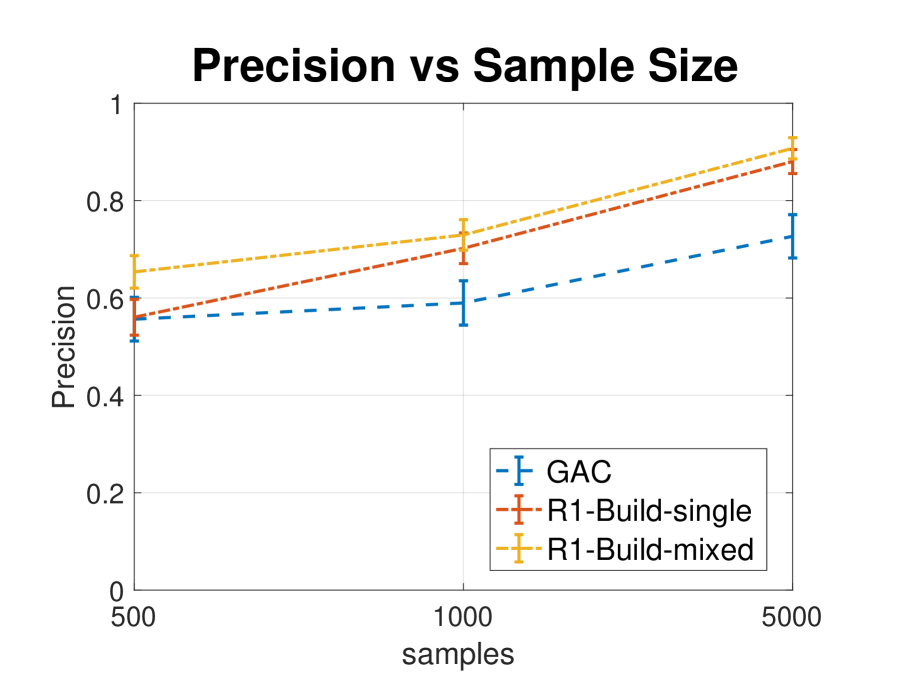
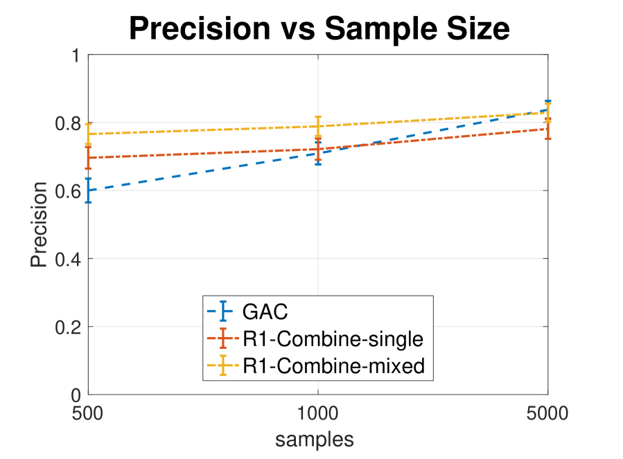
Figure 6: Performance of data-driven methods (R1 Build, R1 Combine) vs. a graphical approach (GAC), measured by precision in finding adjustment sets in data with 500, 1,000, 5,000 samples. Testing thresholds: GAC ($p<.05$), “single” ($p<.05$), “mixed” ($p<0.01$ for $\not\!\perp\!\!\!\!\perp$, $p>0.1$ for $\perp\!\!\!\!\perp$).

In this section, we use simulations to illustrate how our methods perform in settings with multiple treatments. To do this, we simulate data from random DAGs and then attempt to identify an adjustment set using Theorems 5 and 7 on “observed” variables in the generated data. We can verify if these sets are in fact adjustment sets by checking well-known graphical criteria in the data-generating DAG (see Theorem 10 in Supp. A). We compare the performance of our data-driven methods against the performance of an existing graphical approach.

5.1 Specifications

To generate data, we randomly draw 400 causal DAGs over observed treatments $\mathbf{X}={\{X_{1},X_{2}\}}$, outcome $Y$, covariates $\mathbf{W}$, and unobserved $\mathbf{U}$, where ${|\mathbf{W}|=10}$ and ${|\mathbf{U}|=5}$. We require the causal ordering $\mathbf{W}<\mathbf{X}<Y$ to be consistent with each DAG. Then we simulate data from a linear Gaussian model based on each random DAG, with parameters chosen randomly from $[\text{-}1,\text{-}0.1]\cup[0.1,1]$ to avoid very weak correlations. For each DAG, we generate three datasets: one with 500, one with 1,000, and one with 5,000 observations.

Using each dataset, we attempt to find an adjustment set for the causal effect of $\mathbf{X}$ on $Y$. We start by applying Theorems 5 and 7 to the observed data. Then for comparison, we build a causal PAG from the observed data and apply the generalized adjustment criterion of Perković et al. [2018] (GAC; see Theorem 12 in Supp. A). To construct this PAG, we use a causal discovery algorithm known as FciTiers [Andrews et al., 2020] – a version of FCI [Spirtes et al., 2000] that admits temporal knowledge in the form of tiers. Variables can have any causal relationship within tiers, but cannot be causal descendants of downstream tiers. Since the setting we consider assumes ${\mathbf{W}<\mathbf{X}<Y}$, we run FciTiers with three tiers: one for covariates $\mathbf{W}$, one for treatments $\mathbf{X}$, and one for the outcome $Y$.

All three methods introduce error via hypothesis tests for conditional in/dependencies among observed variables. Our methods do this directly in checking the conditions of Theorems 5 and 7. Note that this allows for separate thresholds in tests for dependence versus independence. To take advantage of this, we measure performance of our methods across two settings: using a single threshold (${p<0.05}$) and using a mixed threshold (${p<0.01}$ for dependence, ${p>0.1}$ for independence). The GAC method introduces error indirectly through construction of the causal PAG. We implement FciTiers using a single threshold (${p<.05}$).

To measure performance, we consider how often a method correctly identifies an adjustment set. We compute the precision of a method for a given sample size as $\frac{TP}{TP+FP}$, where $TP$ ($FP$) is the number of true (false) positives out of all generated datasets of the same sample size.

5.2 Results

Figure 6 shows the results of our simulations, where our data-driven methods (R1 Build, R1 Combine) slightly outperform the graphical approach (GAC). We consider two advantages our methods have that may explain this difference in performance. First, our methods do not attempt to identify the model’s entire causal structure and thus avoid errors in hypothesis testing for irrelevant areas of the graph. Further, our methods allow for separate thresholds in testing dependence versus independence, which may improve the reliability of our inferences. In our simulations, using separate thresholds resulted in fewer discoveries but higher accuracy – a trade-off that may be appealing in settings where the cost of false discoveries is high.

While the results of our simulations are encouraging, we note a limitation of our methods in high-dimensional settings. Both Theorems 5 and 7 require a search for variables $W_{i}$, $i\in\{1,\dots,k\}$, that fulfill specific in/dependencies, and Theorem 7 requires additional in/dependence testing in a search for minimal adjustment sets (see Lemma 8). To do this in our simulations, we perform a brute-force search over all possible variables. These searches, which are expensive and require a large number of hypothesis tests, may hinder the applicability of our methods in high-dimensional settings. Future work could address this by exploring greedy-search approaches for implementation.

6 Discussion

This paper considers causal effect identification through covariate adjustment. While prior research in this area focuses on finding adjustment sets based on criteria from a causal graph [Pearl, 1995, Shpitser et al., 2012, Maathuis and Colombo, 2015, Perković et al., 2018], we consider instead a route that relies on conditional in/dependencies in the observed data directly. This extends the work of Entner et al. [2013].

We start by reviewing R1 of Entner et al. [2013] and explaining how c-equivalence can extend this rule. We provide a rationale for such an extension in the context of efficient estimation. Then we present our main contributions: Theorems 5 and 7 (R1 Build and R1 Combine). These data-driven rules parallel R1 of Entner et al. [2013] but in a setting with multiple treatments. Using simulated data, we show that our rules slightly outperform an existing graphical approach, and we note that our methods allow for different thresholds when testing dependence vs. independence – a possible advantage when the cost of false positives is high.

Despite the performance of our rules, we acknowledge their limitations. As shown in Example 6, there are adjustment sets that Theorem 5 cannot find. We resolve this with the introduction of Theorem 7 but make note for researchers who may prefer the intuitiveness of our first rule. Further, as noted in Section 5 Simulations, implementing our rules requires a search for variables that fulfill the theorems’ conditions. Theorem 7 also requires a search for minimality. Future research could explore less expensive search algorithms that improve the applicability of our methods in high-dimensional settings.

Future research could also broaden our extension of Entner et al. [2013] into settings with multiple outcomes or settings with a conditional, rather than a total, causal effect. And we note that our work focuses on extending R1 of Entner et al. [2013] without considering their second rule (R2). Thus, additional work could consider extending R2 to multiple settings as well, where the failure of both extensions might imply an inability to identify the causal effect of interest.

Supplement to:

Data-Driven Adjustment for Multiple Treatments

Contents

1. A Further Preliminaries
   1. A.1 Directed Graphs
   2. A.2 Ancestral Graphs
2. B Proofs for Section : R1 Build
3. C Proofs for Section : R1 Combine
   1. C.1 Main Results
   2. C.2 Supporting Results

Appendix A Further Preliminaries

A.1 Directed Graphs

Proper and Back-door Paths. A path from $\mathbf{X}$ to $\mathbf{Y}$ is proper (with respect to $\mathbf{X}$) if only its first node is in $\mathbf{X}$. A path from $X$ to $Y$ that begins with the edge $X\leftarrow$ is said to be a path into $X$, or a back-door path.

Definition 9

(Back-door Adjustment Set for DAGs; Maathuis and Colombo, 2015) Let $\mathbf{X}$, $\mathbf{Y}$, and $\mathbf{Z}$ be pairwise disjoint node sets in a DAG $\mathcal{D}$. Then $\mathbf{Z}$ is a back-door adjustment set relative to $(\mathbf{X,Y})$ in $\mathcal{D}$ if and only if:

1. $\mathbf{Z}\cap\operatorname{De}(\mathbf{X},\mathcal{D})=\emptyset$, and

2. $\mathbf{Z}\cup\big{[}\mathbf{X}\setminus\{X\}\big{]}$ blocks all back-door paths from $X$ to $\mathbf{Y}$ in $\mathcal{D}$, for all $X\in\mathbf{X}$.

Theorem 10

(Adjustment Set for DAGs, Graphical Criteria; cf. Theorems 3-4 of Shpitser et al., 2012) Let $\mathbf{X}$, $\mathbf{Y}$, and $\mathbf{Z}$ be pairwise disjoint node sets in a causal DAG $\mathcal{D}$. Then $\mathbf{Z}$ is an adjustment set relative to $(\mathbf{X,Y})$ in $\mathcal{D}$ if and only if:

1. $\mathbf{Z}$ contains no descendants of any $W\notin\mathbf{X}$ that lies on a proper causal path from $\mathbf{X}$ to $\mathbf{Y}$ in $\mathcal{D}$, and

2. $\mathbf{Z}$ blocks all non-causal paths from $\mathbf{X}$ to $\mathbf{Y}$ in $\mathcal{D}$.

Lemma 11

(cf. Theorem 3.1 of Maathuis and Colombo, 2015) Let $\mathbf{X}$, $\mathbf{Y}$, and $\mathbf{Z}$ be pairwise disjoint node sets in a causal DAG $\mathcal{D}$. If $\mathbf{Z}$ is a back-door adjustment set relative to $(\mathbf{X,Y})$ in $\mathcal{D}$, then $\mathbf{Z}$ is an adjustment set relative to $(\mathbf{X,Y})$ in $\mathcal{D}$.

A.2 Ancestral Graphs

The following are key definitions related to ancestral graphs and their associated densities. We rely on the framework of Richardson and Spirtes [2002], Zhang [2008], Ali et al. [2009].

Mixed and Partially Directed Mixed Graphs. A mixed graph may contain directed ($\to$) and bi-directed ($\leftrightarrow$) edges. The partially directed mixed graphs we consider may contain directed, bi-directed, undirected (), or partially directed () edges. We use $\bullet$ as a stand in for any edge mark.

Definite Status Paths. Let $\mathcal{G}$ be a mixed or partially directed mixed graph with a path $p:=\langle X_{1},\dots,X_{k}\rangle$, $k>1$. If $p$ contains $X_{j-1}\begin{picture}(5.0,1.0)(0.0,0.0)\put(0.2,0.0){$\bullet$} \put(1.0,0.0){$\rightarrow$} \end{picture}X_{j}\begin{picture}(5.0,1.0)(0.0,0.0)\put(0.2,0.0){$\leftarrow$} \put(3.0,0.0){$\bullet$} \end{picture}X_{j+1}$ for $1<j<k$, then $X_{j}$ is a collider on $p$. $X_{j}$ is a definite non-collider on $p$ if $p$ contains $X_{j-1}\leftarrow X_{j}$ or $X_{j}\rightarrow X_{j+1}$, or if $\mathcal{G}$ contains $X_{j-1}\begin{picture}(5.0,1.0)(0.0,0.0)\put(1.0,1.0){\circle{1.0}} \put(1.5,1.0){\line(1,0){2.0}} \put(4.0,1.0){\circle{1.0}} \end{picture}X_{j}\begin{picture}(5.0,1.0)(0.0,0.0)\put(1.0,1.0){\circle{1.0}} \put(1.5,1.0){\line(1,0){2.0}} \put(4.0,1.0){\circle{1.0}} \end{picture}X_{j+1}$ but no edge $\langle X_{j-1},X_{j+1}\rangle$. If every node on $p$ is a collider, definite non-collider, or endpoint on $p$, then $p$ is a definite status path.

M-connection and M-separation. Let $\mathbf{X}$, $\mathbf{Y}$, and $\mathbf{Z}$ be pairwise disjoint node sets in a mixed or partially directed mixed graph $\mathcal{G}$. A definite-status path $p$ from $\mathbf{X}$ to $\mathbf{Y}$ in $\mathcal{G}$ is open given $\mathbf{Z}$ if every definite non-collider on $p$ is not in $\mathbf{Z}$ and every collider on $p$ has a descendant in $\mathbf{Z}$ in $\mathcal{G}$. Otherwise, $p$ is blocked given $\mathbf{Z}$. If $\mathbf{Z}$ blocks all definite-status paths between $\mathbf{X}$ and $\mathbf{Y}$ in $\mathcal{G}$, then $\mathbf{X}$ is m-separated from $\mathbf{Y}$ given $\mathbf{Z}$ in $\mathcal{G}$ and we write ${(\mathbf{X}\perp_{m}\mathbf{Y}\,|\,\mathbf{Z})_{\mathcal{G}}}$. Otherwise, $\mathbf{X}$ is m-connected to $\mathbf{Y}$ given $\mathbf{Z}$ in $\mathcal{G}$ and we write ${(\mathbf{X}\not\perp_{m}\mathbf{Y}\,|\,\mathbf{Z})_{\mathcal{G}}}$.

MAGs. A directed path from $X$ to $Y$ and the edge $X\to Y$ form an almost directed cycle. A mixed graph without directed or almost directed cycles is called ancestral. Note that we do not consider ancestral graphs that represent selection bias. A maximal ancestral graph (MAG) is an ancestral graph $\mathcal{M}=(\mathbf{V,E})$ where every pair of non-adjacent nodes $X$ and $Y$ in $\mathcal{M}$ can be m-separated by a set $\mathbf{Z}\subseteq\mathbf{V}\setminus\{X,Y\}$. A DAG $\mathcal{D}=(\mathbf{V,E})$ with unobserved variables $\mathbf{U}\subseteq\mathbf{V}$ can be uniquely represented by a MAG $\mathcal{M}=(\mathbf{V}\setminus\mathbf{U},\mathbf{E^{\prime}})$, which preserves the ancestry and m-separations among the observed variables.

PAGs. All MAGs that encode the same set of m-separations form a Markov equivalence class, which can be uniquely represented by a partially directed mixed graph called a partial ancestral graph (PAG). $[\mathcal{G}]$ denotes all MAGs represented by a PAG $\mathcal{G}$. We say a DAG $\mathcal{D}$ is represented by a PAG $\mathcal{G}$ if there is a MAG $\mathcal{M}\in[\mathcal{G}]$ such that $\mathcal{D}$ is represented by $\mathcal{M}$. Note that we only consider maximally informative PAGs that are complete with respect to orientation rules $R1-R4$ and $R8-R10$ of Zhang [2008] and that do not represent selection bias.

Markov Compatibility and Faithfulness. We say an observational density is Markov compatible with a MAG or PAG $\mathcal{G}$ if it is Markov compatible with a DAG represented by $\mathcal{G}$. We say an observational density is faithful to a MAG or PAG $\mathcal{G}$ if it is faithful to a DAG represented by $\mathcal{G}$.

Probabilistic Implications of a Graph. Let $\mathbf{X}$, $\mathbf{Y}$, and $\mathbf{Z}$ be pairwise disjoint node sets in a MAG or PAG $\mathcal{G}$. If ${(\mathbf{X}\perp_{m}\mathbf{Y}\,|\,\mathbf{Z})_{\mathcal{G}}}$, then $\mathbf{X}$ and $\mathbf{Y}$ are independent given $\mathbf{Z}$ in any observational density that is Markov compatible with $\mathcal{G}$. If ${(\mathbf{X}\not\perp_{m}\mathbf{Y}\,|\,\mathbf{Z})_{\mathcal{G}}}$, then $\mathbf{X}$ and $\mathbf{Y}$ are dependent given $\mathbf{Z}$ in any observational density that is faithful to $\mathcal{G}$.

Causal Graphs. Let $\mathcal{G}$ be a graph with nodes $V_{i}$ and $V_{j}$. When $\mathcal{G}$ is a MAG or PAG, it is a causal MAG or causal PAG if every edge $V_{i}\to V_{j}$ represents the presence of a causal path from $V_{i}$ to $V_{j}$; every edge $V_{i}\begin{picture}(5.0,1.0)(0.0,0.0)\put(0.2,0.0){$\leftarrow$} \put(3.0,0.0){$\bullet$} \end{picture}V_{j}$ represents the absence of a causal path from $V_{i}$ to $V_{j}$; and every edge $V_{i}\begin{picture}(5.0,1.0)(0.0,0.0)\put(1.0,1.0){\circle{1.0}} \put(1.5,1.0){\line(1,0){2.0}} \put(4.0,1.0){\circle{1.0}} \end{picture}V_{j}$ represents the presence of a causal path of unknown direction or a common cause in the underlying causal DAG.

Possibly Causal Paths. Let $p:=\langle X_{1},\dots,X_{k}\rangle$, $k>1$, be a path in a causal MAG or PAG $\mathcal{G}$. If $\mathcal{G}$ does not contain an edge $X_{i}\begin{picture}(5.0,1.0)(0.0,0.0)\put(0.2,0.0){$\leftarrow$} \put(3.0,0.0){$\bullet$} \end{picture}X_{j},1\leq i<j\leq k$, then $p$ is possibly causal and $X_{2},\dots,X_{k}$ are possible descendants of $X_{1}$. Otherwise, $p$ is non-causal.

Visible Edges. Let $\mathcal{G}$ be a MAG or PAG. We denote that $X$ is adjacent to $Y$ in $\mathcal{G}$ by $X\in\operatorname{Adj}(Y,\mathcal{G})$. A directed edge $X\rightarrow Y$ is visible in $\mathcal{G}$ if there is a node $V\notin\operatorname{Adj}(Y,\mathcal{G})$ such that $\mathcal{G}$ contains either $V\begin{picture}(5.0,1.0)(0.0,0.0)\put(0.2,0.0){$\bullet$} \put(1.0,0.0){$\rightarrow$} \end{picture}X$ or $V\begin{picture}(5.0,1.0)(0.0,0.0)\put(0.2,0.0){$\bullet$} \put(1.0,0.0){$\rightarrow$} \end{picture}V_{1}\leftrightarrow\dots\leftrightarrow V_{k}\leftrightarrow X$, where $k\geq 1$ and $V_{1},\dots,V_{k}\in\operatorname{Pa}(Y,\mathcal{G})\setminus\{V,X,Y\}$.

Consistency. We say an interventional density is consistent with a causal MAG or PAG $\mathcal{G}$ if it is consistent with each DAG represented by $\mathcal{G}$ – were the DAG to be causal.

Adjustment Sets. Let $\mathbf{X}$, $\mathbf{Y}$, and $\mathbf{Z}$ be pairwise disjoint node sets in a causal MAG or PAG $\mathcal{G}$. Then $\mathbf{Z}$ is an adjustment set relative to $(\mathbf{X,Y})$ in $\mathcal{G}$ if and only if $f(\mathbf{y}|do(\mathbf{x}))=\int f(\mathbf{y}|\mathbf{x},\mathbf{z})f(\mathbf{z})\mathop{}\!\mathrm{d}\mathbf{z}$ for any $f$ consistent with $\mathcal{G}$. We omit reference to $(\mathbf{X,Y})$ or $\mathcal{G}$ when it can be assumed.

Theorem 12

(Adjustment Set for PAGs, Graphical Criteria; cf. Theorem 5 of Perković et al., 2018) Let $\mathbf{X}$, $\mathbf{Y}$, and $\mathbf{Z}$ be pairwise disjoint node sets in a causal PAG $\mathcal{G}$. Then $\mathbf{Z}$ is an adjustment set relative to $(\mathbf{X},\mathbf{Y})$ in $\mathcal{G}$ if and only if

1. every proper, possibly causal path from $\mathbf{X}$ to $\mathbf{Y}$ in $\mathcal{G}$ starts with a visible edge,

2. $\mathbf{Z}$ contains no possible descendants of any $W\notin\mathbf{X}$ that lies on a proper, possibly causal path from $\mathbf{X}$ to $\mathbf{Y}$ in $\mathcal{G}$, and

3. $\mathbf{Z}$ blocks all proper, definite status, non-causal paths from $\mathbf{X}$ to $\mathbf{Y}$ in $\mathcal{G}$.

Appendix B Proofs for Section 4.1 Building on Adjustment Sets: R1 Build

• The result holds for $k=1$ by Theorem 1. Thus, let $k\geq 2$. Suppose there exist $W_{1},\dots,W_{k}\in\mathbf{W}$ and $\mathbf{Z}\subseteq\mathbf{W}\setminus\{W_{1},\dots,W_{k}\}$ such that (i) and (ii) hold for $i\in\{1,\dots,k\}$. Let $\mathcal{D}$ be the DAG induced by the causal model. Then for ease of notation, let $\mathbf{X^{N}_{i}}=\mathbf{X}\setminus\operatorname{De}(X_{i},\mathcal{D})$, and note that $\{X_{1},\dots,X_{i}\}^{-i}\subseteq\mathbf{X^{N}_{i}}$ since $X_{1}<\dots<X_{k}$ is a causal ordering consistent with the model.

  We start by showing that $\mathbf{X}$ has a causal effect on $Y$. Consider an arbitrary $j\in\{1,\dots,k\}$. By (i), (ii), and faithfulness, there must be a path $p_{j}$ from $W_{j}$ to $Y$ in $\mathcal{D}$ that is open given $\mathbf{Z}\cup\{X_{1},\dots,X_{j}\}^{-j}$ and contains $X_{j}$ as a non-collider. Therefore, either $p_{j}(W_{j},X_{j})$ ends $\leftarrow X_{j}$ or $p_{j}(X_{j},Y)$ begins $X_{j}\to$. For sake of contradiction, suppose the former holds. Since $X_{j}\notin\operatorname{An}(\mathbf{W},\mathcal{D})$, then $p_{j}(W_{j},X_{j})$ must contain a collider. But since $p_{j}$ is open given $\mathbf{Z}\cup\{X_{1},\dots,X_{j}\}^{-j}\subseteq\mathbf{W}\cup\mathbf{X_{j}^{N}}$, the closest collider to $X_{j}$ on $p_{j}(W_{j},X_{j})$ must be in $\operatorname{An}(\mathbf{Z}\cup\{X_{1},\dots,X_{j}\}^{-j},\,\,\mathcal{D})$, which contradicts that $X_{j}\notin\operatorname{An}(\mathbf{W}\cup\mathbf{X_{j}^{N}},\mathcal{D})$. Thus, $p_{j}(X_{j},Y)$ must begin $X_{j}\to$. By similar logic, $p_{j}(X_{j},Y)$ cannot contain a collider, and so $p_{j}$ must end $\to X_{j}\to\dots\to Y$.

  We continue by showing that $\mathbf{Z}$ satisfies the conditions of Definition 9 and thus by Lemma 11, is an adjustment set relative to $(\mathbf{X},Y)$. By assumption, no variable in $\mathbf{Z}$ is a descendant of $\mathbf{X}$. Thus, we only need to show the following for $i\in\{1,\dots,k\}$:

  $$\mathbf{Z}\cup\mathbf{X^{\text{-}i}}\text{ blocks ever} \ast$$ y back-door path ()

  $$\text{from }X_{i}\text{ to} \text{ }Y\text{ in }\mathcal{D}.$$

  We begin with $i=k$, and proceed with a proof by induction for $i\in\{1,\dots,k-1\}$.

BASE CASE: Note from the discussion above that there must be a path $p_{k}$ from $W_{k}$ to $Y$ in $\mathcal{D}$ that is open given $\mathbf{Z}\cup\mathbf{X}^{-k}$ and ends $\to X_{k}\to\dots\to Y$. Then for sake of contradiction, suppose there is a back-door path $q_{k}$ from $X_{k}$ to $Y$ in $\mathcal{D}$ that is open given $\mathbf{Z}\cup\mathbf{X^{\text{-}k}}$. Let $A$ be the node on both $p_{k}$ and $q_{k}$ that is closest to $W_{k}$ on $p_{k}$, and define $r_{k}=p_{k}(W_{k},A)\oplus q_{k}(A,Y)$. We show below that $r_{k}$ must be open given $\mathbf{Z}\cup\mathbf{X}$ – that is, no non-collider on $r_{k}$ is in $\mathbf{Z}\cup\mathbf{X}$ and every collider on $r_{k}$ is in $\operatorname{An}\big{(}\mathbf{Z}\cup\mathbf{X},\mathcal{D}\big{)}$ – which contradicts (ii) by faithfulness.

First consider the nodes on $r_{k}$ other than $A$. Every collider on $r_{k}(W_{k},A)$ and $r_{k}(A,Y)$ is in $\operatorname{An}\big{(}\mathbf{Z}\cup\mathbf{X},\mathcal{D}\big{)}$, since $p_{k}$ and $q_{k}$ are open given $\mathbf{Z}\cup\mathbf{X^{\text{-}k}}$. By the same logic, no non-collider on $r_{k}(W_{k},A)$ or $r_{k}(A,Y)$ is in $\mathbf{Z}\cup\mathbf{X^{\text{-}k}}$. Further, $X_{k}$ is not a non-collider on $r_{k}(W_{k},A)$ or $r_{k}(A,Y)$, since $r_{k}$ does not contain $X_{k}$ except possibly $A=X_{k}$.

Next consider the node $A$. When $A=W_{k}$, note that $r_{k}=r_{k}(A,Y)$, and the base case is done. When $A\neq W_{k}$, we show in the cases below that $A$ is either a collider on $r_{k}$ such that $A\in\operatorname{An}\big{(}\mathbf{Z}\cup\mathbf{X},\mathcal{D}\big{)}$ or a non-collider on $r_{k}$ such that $A\notin\mathbf{Z}\cup\mathbf{X}$, which completes the base case.

• Let $A=X_{k}$. Note that $A$ is a collider on $r_{k}$ (by definition of $p_{k}$ and $q_{k}$) and $A\in\operatorname{An}\big{(}\mathbf{Z}\cup\mathbf{X},\mathcal{D}\big{)}$.

• Let $A\in\mathbf{Z}\cup\mathbf{X^{\text{-}k}}$. Since $p_{k}$ and $q_{k}$ are open given $\mathbf{Z}\cup\mathbf{X^{\text{-}k}}$, then $A$ must be a collider on both paths. Therefore, $A$ is a collider on $r_{k}$ and $A\in\operatorname{An}\big{(}\mathbf{Z}\cup\mathbf{X},\mathcal{D}\big{)}$.

• Let $A\notin\mathbf{Z}\cup\mathbf{X}$. When $A$ is a non-collider on $r_{k}$, the claim holds. When $A$ is a collider on $r_{k}$, we only need to show that $A\in\operatorname{An}(\mathbf{Z}\cup\mathbf{X},\mathcal{D})$. This holds if $A$ is a collider on $p_{k}$, since $p_{k}$ is open given $\mathbf{Z}\cup\mathbf{X^{\text{-}k}}$. Consider when $A$ is a collider on $r_{k}$ and a non-collider on $p_{k}$. Note that $p_{k}(W_{k},X_{k})$ begins $W_{k}\dots\to A\to$ and ends $\to X_{k}$. When $p_{k}(A,X_{k})$ is directed, then $A\in\operatorname{An}(\mathbf{Z}\cup\mathbf{X},\mathcal{D})$. When $p_{k}(A,X_{k})$ contains a collider, the earliest such collider must be in $\operatorname{An}(\mathbf{Z}\cup\mathbf{X^{\text{-}k}},\mathcal{D})$, since $p_{k}$ is open given $\mathbf{Z}\cup\mathbf{X^{\text{-}k}}$. Thus, $A\in\operatorname{An}(\mathbf{Z}\cup\mathbf{X},\mathcal{D})$.

INDUCTION: Pick an arbitrary $j\in\{1,\dots,k-1\}$, and for sake of induction, assume that ($\ast$ ‣ B) holds for $i\in\{j+1,\dots,k\}$. We will show that ($\ast$ ‣ B) also holds for $i=j$.

Recall that there must be a path $p_{j}$ from $W_{j}$ to $Y$ in $\mathcal{D}$ that is open given $\mathbf{Z}\cup\{X_{1},\dots,X_{j}\}^{-j}$ and ends $\to X_{j}\to\dots\to Y$. Then for sake of contradiction, suppose there is a back-door path $q_{j}$ from $X_{j}$ to $Y$ in $\mathcal{D}$ that is open given $\mathbf{Z}\cup\mathbf{X^{\text{-}j}}$. Let $B$ be the node on both $p_{j}$ and $q_{j}$ that is closest to $W_{j}$ on $p_{j}$, and define $r_{j}=p_{j}(W_{j},B)\oplus q_{j}(B,Y)$. We show below that $r_{j}$ must be open given $\mathbf{Z}\cup\{X_{1},\dots,X_{j}\}$ – that is, no non-collider on $r_{j}$ is in $\mathbf{Z}\cup\{X_{1},\dots,X_{j}\}$ and every collider on $r_{j}$ is in $\operatorname{An}\big{(}\mathbf{Z}\cup\{X_{1},\dots,X_{j}\},\mathcal{D}\big{)}$ – which contradicts (ii) by faithfulness.

First consider the nodes on $r_{j}(W_{j},B)$. Every collider on $r_{j}(W_{j},B)$ is in $\operatorname{An}\big{(}\mathbf{Z}\cup\{X_{1},\dots,X_{j}\},\mathcal{D}\big{)}$, since $p_{j}$ is open given $\mathbf{Z}\cup\{X_{1},\dots,X_{j}\}^{\text{-}j}$. By the same logic and the fact that $r_{j}$ does not contain $X_{j}$ except possibly $B=X_{j}$, no non-collider on $r_{j}(W_{j},B)$ is in $\mathbf{Z}\cup\{X_{1},\dots,X_{j}\}$.

Next consider the nodes on $r_{j}(B,Y)$. No non-collider on $r_{j}(B,Y)$ is in $\mathbf{Z}\cup\{X_{1},\dots,X_{j}\}$, since $q_{j}$ is open given $\mathbf{Z}\cup\mathbf{X^{\text{-}j}}$ and $X_{j}$ is an endpoint on $q_{j}$. Then suppose for sake of contradiction that there is a collider on $r_{j}(B,Y)$ not in $\operatorname{An}\big{(}\mathbf{Z}\cup\{X_{1},\dots,X_{j}\},\mathcal{D}\big{)}$, and let $C$ be the closest such collider to $Y$ on $r_{j}(B,Y)$. Note that $C\in\operatorname{An}(\{X_{j+1},\dots,X_{k}\},\mathcal{D})$, since $q_{j}$ is open given $\mathbf{Z}\cup\mathbf{X^{\text{-}j}}$. Thus, let $s$ be a shortest directed path in $\mathcal{D}$ from $C$ to $\{X_{j+1},\dots,X_{k}\}$, where we denote the latter endpoint $X_{\ell}$, $\ell\in\{j+1,\dots,k\}$. Then let $E$ be the node on both $s$ and $r_{j}$ that is closest to $Y$ on $r_{j}$.

Consider the path $t=s(X_{\ell},E)\oplus r_{j}(E,Y)$. Start by noting that no non-collider on $t$ is in $\mathbf{Z}\cup\mathbf{X^{\text{-}\ell}}$ due to the following: $C\notin\operatorname{An}\big{(}\mathbf{Z}\cup\{X_{1},\dots,X_{j}\},\mathcal{D}\big{)}$; $s$ is a shortest path to $\{X_{j+1},\dots,X_{k}\}$; $q_{j}$ is open given $\mathbf{Z}\cup\mathbf{X^{\text{-}j}}$; and $X_{j}$ is an endpoint on $q_{j}$. Further, every collider on $t$ must be in $\operatorname{An}(\mathbf{Z}\cup\mathbf{X^{\text{-}\ell}},\mathcal{D})$, since $t$ can only contain colliders that are colliders on $r_{j}(E,Y)$, where by definition of $C$, every collider on $r_{j}(E,Y)$ is in $\operatorname{An}\big{(}\mathbf{Z}\cup\{X_{1},\dots,X_{j}\},\mathcal{D}\big{)}$. Thus, $t$ – a back-door path from $X_{\ell}$ to $Y$ – is open given $\mathbf{Z}\cup\mathbf{X^{\text{-}\ell}}$, which contradicts our induction assumption that ($\ast$ ‣ B) holds for $i=\ell$, $\ell\in\{j+1,\dots,k\}$.

Finally, consider the node $B$. When $B=W_{j}$, note that $r_{j}=r_{j}(B,Y)$, and the induction step is done. When $B\neq W_{j}$, we show in the cases below that $B$ is either a collider on $r_{j}$ such that $B\in\operatorname{An}\big{(}\mathbf{Z}\cup\{X_{1},\dots,X_{j}\},\mathcal{D}\big{)}$ or a non-collider on $r_{j}$ such that $B\notin\mathbf{Z}\cup\{X_{1},\dots,X_{j}\}$, which completes the proof.

• Let $B=X_{j}$. Note that $B$ is a collider on $r_{j}$ (by definition of $p_{j}$ and $q_{j}$) and $B\in\operatorname{An}\big{(}\mathbf{Z}\cup\{X_{1},\dots,X_{j}\},\mathcal{D}\big{)}$.

• Let $B\in\mathbf{Z}\cup\{X_{1},\dots,X_{j}\}^{\text{-}j}$. Since $p_{j}$ is open given $\mathbf{Z}\cup\{X_{1},\dots,X_{j}\}^{\text{-}j}$ and $q_{j}$ is open given $\mathbf{Z}\cup\mathbf{X^{\text{-}j}}$, then $B$ must be a collider on both paths. Therefore, $B$ is a collider on $r_{j}$ and $B\in\operatorname{An}\big{(}\mathbf{Z}\cup\{X_{1},\dots,X_{j}\},\mathcal{D}\big{)}$.

• For sake of contradiction, let $B=X_{\ell}$, $\ell\in\{j+1,\dots,k\}$. Note that $B$ must be a collider on $q_{j}$, since $q_{j}$ is open given $\mathbf{Z}\cup\mathbf{X^{\text{-}j}}$. Thus, $r_{j}(B,Y)$ is a back-door path from $X_{\ell}$ to $Y$. However, note that no non-collider on $r_{j}(B,Y)$ is in $\mathbf{Z}\cup\mathbf{X^{\text{-}\ell}}$, since $q_{j}$ is open given $\mathbf{Z}\cup\mathbf{X^{\text{-}j}}$ and since $X_{j}$ is an endpoint on $q_{j}$. Further, every collider on $r_{j}(B,Y)$ is in $\operatorname{An}\big{(}\mathbf{Z}\cup\mathbf{X^{\text{-}\ell}},\mathcal{D}\big{)}$, since we have shown that every collider on $r_{j}(B,Y)$ is in $\operatorname{An}\big{(}\mathbf{Z}\cup\{X_{1},\dots,X_{j}\},\mathcal{D}\big{)}$. Therefore, $r_{j}(B,Y)$ is a back-door path from $X_{\ell}$ to $Y$ that is open given $\mathbf{Z}\cup\mathbf{X^{\text{-}\ell}}$, which contradicts our induction assumption that ($\ast$ ‣ B) holds for $i=\ell$, $\ell\in\{j+1,\dots,k\}$.

• Let $B\notin\mathbf{Z}\cup\mathbf{X}$. When $B$ is a non-collider on $r_{j}$, the claim holds. When $B$ is a collider on $r_{j}$, we only need to show that $B\in\operatorname{An}\big{(}\mathbf{Z}\cup\{X_{1},\dots,X_{j}\},\mathcal{D}\big{)}$. This holds if $B$ is also a collider on $p_{j}$, since $p_{j}$ is open given $\mathbf{Z}\cup\{X_{1},\dots,X_{j}\}^{\text{-}j}$. Consider when $B$ is a collider on $r_{j}$ and a non-collider on $p_{j}$. Note that $p_{j}(W_{j},X_{j})$ begins $W_{j}\dots\to B\to$ and ends $\to X_{j}$. When $p_{j}(B,X_{j})$ is directed, then $B\in\operatorname{An}\big{(}\mathbf{Z}\cup\{X_{1},\dots,X_{j}\},\mathcal{D}\big{)}$. When $p_{j}(B,X_{j})$ contains a collider, the earliest such collider must be in $\operatorname{An}(\mathbf{Z}\cup\{X_{1},\dots,X_{j}\}^{\text{-}j},\mathcal{D})$, since $p_{j}$ is open given $\mathbf{Z}\cup\{X_{1},\dots,X_{j}\}^{\text{-}j}$. Thus, $B\in\operatorname{An}\big{(}\mathbf{Z}\cup\{X_{1},\dots,X_{j}\},\mathcal{D}\big{)}$.

 

Appendix C Proofs for Section 4.2 Combining Adjustment Sets: R1 Combine

C.1 Main Results

• The result holds for $k=1$ by Theorem 1. Thus, let $k\geq 2$. Suppose there exist $W_{1},\dots,W_{k}\in\mathbf{W}$ and $\mathbf{T_{i}}\subseteq\big{[}\mathbf{W}\setminus\{W_{1},\dots,W_{k}\}\big{]}\cup\mathbf{X^{N}_{i}}$ such that (i)-(ii) hold for all $i\in\{1,\dots,k\}$. Note by (i), (ii), and Theorem 1 that $X_{i}$ has a causal effect on $Y$ that is identifiable through the adjustment set $\mathbf{T_{i}}$. Thus, $\mathbf{X}$ has a causal effect on $Y$, and we can define $\mathbf{Z_{i}}$ to be any minimal adjustment set relative to $(X_{i},Y)$ such that $\mathbf{Z_{i}}\subseteq\mathbf{T_{i}}$. Let $\mathcal{D}$ be the DAG induced by the causal model so that $\mathbf{X^{N}_{i}}=\mathbf{X}\setminus\operatorname{De}(X_{i},\mathcal{D})$. Then for ease of notation, let $\mathbf{X^{\text{-}i}}=\mathbf{X}\setminus\{X_{i}\}$.

  We show below that $\mathbf{Z}:=\cup_{i=1}^{k}\mathbf{Z_{i}}\setminus\mathbf{X}$ satisfies the conditions of Definition 9 and thus by Lemma 11, is an adjustment set relative to $(\mathbf{X},Y)$. Since $\mathbf{Z}\subseteq\mathbf{W}$ where $\mathbf{W}<\mathbf{X}$, we only need to show for every $i\in\{1,\dots,k\}$ that $\mathbf{Z}\cup\mathbf{X^{\text{-}i}}$ blocks every back-door path from $X_{i}$ to $Y$ in $\mathcal{D}$. Without loss of generality, we show this holds for $i=1$.

  For sake of contradiction, suppose there is a back-door path $q$ from $X_{1}$ to $Y$ in $\mathcal{D}$ that is open given $\mathbf{Z}\cup\mathbf{X^{\text{-}1}}$. Since $\mathbf{Z_{1}}$ is an adjustment set relative to $(X_{1},Y)$, then by Theorem 10, $q$ must be blocked given $\mathbf{Z_{1}}\subseteq\mathbf{Z}\cup\mathbf{X^{\text{-}1}}$. This implies that $q$ must contain a collider in $\operatorname{An}\big{(}\mathbf{Z}\cup\mathbf{X^{\text{-}1}},\mathcal{D}\big{)}\setminus\operatorname{An}(\mathbf{Z_{1}},\mathcal{D})$. Let $C_{1},\dots,C_{\ell}$, $\ell\geq 1$, be the set of all such colliders – ordered so that $C_{1}$ is the closest such collider to $X_{1}$ on $q$ and $C_{\ell}$ is the furthest such collider from $X_{1}$ on $q$.

  We pause to define a path $t_{i}$ in $\mathcal{D}$ that is directed from $C_{i}$ to $Y$ for any $i\in\{1,\dots,\ell\}$ such that $C_{i}\notin\operatorname{An}(X_{1},\mathcal{D})$. This path will be useful in showing a contradiction. First pick such an $i\in\{1,\dots,\ell\}$ (supposing one exists), and define $r_{i}$ as a longest directed path from $C_{i}$ to $\big{(}\mathbf{Z}\cup\mathbf{X^{\text{-}1}}\big{)}\setminus\operatorname{An}(\mathbf{Z_{1}},\mathcal{D})$ in $\mathcal{D}$. Then define $t_{i}$ based on how $r_{i}$ ends.

  When $r_{i}$ ends with $X_{j}\in\mathbf{X^{\text{-}1}}\setminus\operatorname{An}(\mathbf{Z_{1}},\mathcal{D})$ for some $j\in\{2,\dots,k\}$, note that by (i), (ii), and faithfulness, there must be a path $p_{j}$ from $W_{j}$ to $Y$ in $\mathcal{D}$ that is open given $\mathbf{T_{j}}$ and contains $X_{j}$ as a non-collider. Therefore, either $p_{j}(W_{j},X_{j})$ ends $\leftarrow X_{j}$ or $p_{j}(X_{j},Y)$ begins $X_{j}\to$. For sake of contradiction, suppose the former holds. Since $X_{j}\notin\operatorname{An}(\mathbf{W},\mathcal{D})$, then $p_{j}(W_{j},X_{j})$ must contain a collider. But since $p_{j}$ is open given $\mathbf{T_{j}}\subseteq\mathbf{W}\cup\mathbf{X_{j}^{N}}$, the closest collider to $X_{j}$ on $p_{j}(W_{j},X_{j})$ must be in $\operatorname{An}(\mathbf{T_{j}},\mathcal{D})$, which contradicts that $X_{j}\notin\operatorname{An}(\mathbf{W}\cup\mathbf{X_{j}^{N}},\mathcal{D})$. Thus, $p_{j}(X_{j},Y)$ must begin $X_{j}\to$. By similar logic, $p_{j}(X_{j},Y)$ cannot contain a collider, and so $p_{j}(X_{j},Y)$ must take the form $X_{j}\to\dots\to Y$. Thus, we can define $t_{i}=r_{i}\oplus p_{j}(X_{j},Y)$.

  Next, consider when $r_{i}$ ends with $Z_{j}\in\mathbf{Z}\setminus\operatorname{An}(\mathbf{Z_{1}},\mathcal{D})$ so that $Z_{j}\in\mathbf{Z_{j}}\setminus\mathbf{X}$ for some $j\in\{2,\dots,k\}$. By definition, $\mathbf{Z_{j}}$ is an adjustment set relative to $(X_{j},Y)$, but this does not hold for any subset $\mathbf{Z_{j}}\setminus\{Z\}$, where $Z\in\mathbf{Z_{j}}$. Thus by Theorem 10, there must be a non-causal path from $X_{j}$ to $Y$ in $\mathcal{D}$ that contains $Z_{j}$ as a non-collider and that is open given $\mathbf{Z_{j}}\setminus\{Z_{j}\}$. Let $s_{j}$ be one such path. For sake of contradiction, suppose $s_{j}(Z_{j},Y)$ begins $Z_{j}\leftarrow$. Since $Z_{j}$ is a non-collider on $s_{j}$, then $s_{j}(X_{j},Z_{j})$ must end with $\leftarrow Z_{j}$. If $s_{j}(X_{j},Z_{j})$ contains a collider, then by the definition of $s_{j}$, the closest such collider to $Z_{j}$ on $s_{j}$ must be in $\operatorname{An}(\mathbf{Z_{j}}\setminus\{Z_{j}\},\mathcal{D})$, which contradicts either the definition of $r_{i}$ as a longest path to $\big{(}\mathbf{Z}\cup\mathbf{X^{\text{-}1}}\big{)}\setminus\operatorname{An}(\mathbf{Z_{1}},\mathcal{D})$ or the definition of $C_{i}\notin\operatorname{An}(\mathbf{Z_{1}}\cup\{X_{1}\},\mathcal{D})$. The same contradiction holds if instead $s_{j}(X_{j},Z_{j})$ takes the form $X_{j}\leftarrow\dots\leftarrow Z_{j}$. Therefore, $s_{j}(Z_{j},Y)$ must begin $Z_{j}\to$. Further, $s_{j}(Z_{j},Y)$ must take the form $Z_{j}\to\dots\to Y$, since by the same logic, $s_{j}(Z_{j},Y)$ cannot contain a collider. Thus, here we define $t_{i}=r_{i}\oplus s_{j}(Z_{j},Y)$.

  We proceed to cases with a directed path from $C_{i}$ to $Y$ defined as follows:

  $$t_{i}:=\begin{cases}r_{i}\oplus p_{j}(X_{j},Y)&r_{i}\text{ ends }X_{j}\in\mathbf{X^{\text{-}1}}\setminus\operatorname{An}(\mathbf{Z_{1}},\mathcal{D})\\ r_{i}\oplus s_{j}(Z_{j},Y)&r_{i}\text{ ends }Z_{j}\in\mathbf{Z}\setminus\operatorname{An}(\mathbf{Z_{1}},\mathcal{D}).\end{cases}$$

  We use this path in the cases below to show there must be a non-causal path $u$ from $X_{1}$ to $Y$ in $\mathcal{D}$ that is open given $\mathbf{Z_{1}}$, which by Theorem 10, contradicts that $\mathbf{Z_{1}}$ is an adjustment set relative to $(X_{1},Y)$.

CASE 1: Suppose there is no directed path from $\{C_{1},\dots,C_{\ell}\}$ to $X_{1}$ in $\mathcal{D}$. Therefore, consider $C_{1}$ and its corresponding path $t_{1}$. Note that $q(X_{1},C_{1})$ and $t_{1}$ cannot share a node other than $C_{1}$, since any such node would have a directed path (possibly of length zero) in $\mathcal{D}$ to $C_{1}$, $X_{1}$, or a collider on $q(X_{1},C_{1})$. And this would contradict the acyclicity of $\mathcal{D}$, the fact that there is no directed path from $\{C_{1},\dots,C_{\ell}\}$ to $X_{1}$ in $\mathcal{D}$, or the definition of $C_{1}\notin\operatorname{An}(\mathbf{Z_{1}},\mathcal{D})$ as the closest such collider to $X_{1}$ on $q$. Thus, we can consider the path $u:=q(X_{1},C_{1})\oplus t_{1}$. Note that $q(X_{1},C_{1})$ is open given $\mathbf{Z_{1}}$ by the definition of $q$ and $C_{1}$. Further by the definition of $C_{1}$ and $t_{1}$, no node on $t_{1}$ is in $\mathbf{Z_{1}}$ and every node on $t_{1}$ is a non-collider on $u$. Therefore, $u$ – a non-causal path in $\mathcal{D}$ from $X_{1}$ to $Y$ – is open given $\mathbf{Z_{1}}$, which is a contradiction.

CASE 2: Suppose there is a directed path from $\{C_{1},\dots,C_{\ell}\}$ to $X_{1}$ in $\mathcal{D}$. Let $C_{a}$, $a\in\{1,\dots,\ell\}$, be the closest such collider to $Y$ on $q$, let $w$ be an arbitrary directed path from $C_{a}$ to $X_{1}$ in $\mathcal{D}$, and let $A$ be the node on both $q$ and $w$ that is closest to $Y$ on $q$.

When $A$ is a node on $q(C_{\ell},Y)$, consider the path $u:=(-w)(X_{1},A)\oplus q(A,Y)$. Note by the definition of $C_{a}$ and $w$ that no node on $(-w)(X_{1},A)$ is in $\mathbf{Z_{1}}$ and every node on $(-w)(X_{1},A)$ is a non-collider on $u$. Further note that $q(A,Y)$ is open given $\mathbf{Z_{1}}$ by the definition of $q$ and $C_{\ell}$. Therefore, $u$ – a non-causal path in $\mathcal{D}$ from $X_{1}$ to $Y$ – is open given $\mathbf{Z_{1}}$, which is a contradiction.

When $A$ precedes $C_{\ell}$ on $q$, let $C_{b}$ be the collider in $\{C_{a+1},\dots,C_{\ell}\}$ closest to $A$ on $q(A,Y)$. Note by the definition of $C_{a}$ that $C_{b}\notin\operatorname{An}(X_{1},\mathcal{D})$. Therefore, we can consider the path $t_{b}$, which is directed from $C_{b}$ to $Y$. Note that $(-w)(X_{1},A)\oplus q(A,C_{b})$ and $t_{b}$ cannot share a node other than $C_{b}$, since any such node would have a directed path (possibly of length zero) in $\mathcal{D}$ to $C_{b}$, $X_{1}$, or a collider on $q(A,C_{b})$. And this would contradict the acyclicity of $\mathcal{D}$, the definition of $C_{a}$ as the closest collider in $\{C_{1},\dots,C_{\ell}\}$ to $Y$ on $q$ with a directed path to $X_{1}$, or the definition of $C_{b}\notin\operatorname{An}(\mathbf{Z_{1}},\mathcal{D})$ as the closest such collider to $A$ on $q(A,Y)$. Thus, we can consider the path $u:=(-w)(X_{1},A)\oplus q(A,C_{b})\oplus t_{b}$. Note by the definition of $C_{a}$ and $w$ that no node on $(-w)(X_{1},A)$ is in $\mathbf{Z_{1}}$ and every node on $(-w)(X_{1},A)$ is a non-collider on $u$. The same holds for $t_{b}$ by analogous logic. Further, note that $q(A,C_{b})$ is open given $\mathbf{Z_{1}}$ by the definition of $q$, $A$, and $C_{b}$. Therefore, $u$ – a non-causal path in $\mathcal{D}$ from $X_{1}$ to $Y$ – is open given $\mathbf{Z_{1}}$, which is a contradiction.  

• Let $\mathbf{T}$ be an adjustment set relative to $(X,Y)$ in a causal model where $\mathbf{T}<X$. Then by Lemmas 14-15, $\mathbf{T}$ is a minimal adjustment set relative to $(X,Y)$ if and only if (i)-(ii) hold for all $T\in\mathbf{T}$.

  When (i) or (ii) do not hold for some $T\in\mathbf{T}$, let $\mathbf{Z}$ be a proper subset of $\mathbf{T}$ such that (iii)-(v) hold for all $Z\in\mathbf{Z}$. In addition to (v), note that trivially $X\perp\!\!\!\!\perp\mathbf{Z}\,|\,\mathbf{T}$ and $Y\perp\!\!\!\!\perp\mathbf{Z}\,|\,\mathbf{T}\cup\{X\}$, since $\mathbf{Z}\subset\mathbf{T}$. Therefore, by Theorem 3, $\mathbf{Z}$ is c-equivalent to $\mathbf{T}$ and thus, is an adjustment set relative to $(X,Y)$. Then, as above, $\mathbf{Z}$ is minimal by (iii)-(iv) and Lemmas 14-15.  

C.2 Supporting Results

Definition 13

(Elementwise Minimal Adjustment Set) A set $\mathbf{Z}$ is an elementwise minimal adjustment set relative to $(\mathbf{X},\mathbf{Y})$ if $\mathbf{Z}$ is an adjustment set relative to $(\mathbf{X},\mathbf{Y})$ and if $\mathbf{Z}\setminus\{Z\}$ is not an adjustment set relative to $(\mathbf{X},\mathbf{Y})$ for any $Z\in\mathbf{Z}$.

Lemma 14 (Criteria for Elementwise Minimality)

Let $\mathbf{Z}$ be an adjustment set relative to $(\mathbf{X},\mathbf{Y})$ in a causal model where $\mathbf{Z}<\mathbf{X}$. Then $\mathbf{Z}$ is an elementwise minimal adjustment set relative to $(\mathbf{X},\mathbf{Y})$ if and only if the following hold for some $X\in\mathbf{X}$, $Y\in\mathbf{Y}$, and for all $Z\in\mathbf{Z}$:

1. $X\not\!\perp\!\!\!\!\perp Z\,\big{|}\,\mathbf{Z}\setminus\{Z\}$,   and

2. $Y\not\!\perp\!\!\!\!\perp Z\,\big{|}\,\big{[}\mathbf{Z}\setminus\{Z\}\big{]}\cup\{X\}$.

• Let $\mathbf{X}$, $\mathbf{Y}$, and $\mathbf{Z}$ be pairwise disjoint node sets in a causal DAG $\mathcal{D}$, where $\mathbf{Z}$ is an adjustment set relative to $(\mathbf{X},\mathbf{Y})$ in $\mathcal{D}$ and where $\mathbf{Z}<\mathbf{X}$.

  $\Rightarrow$ Let $\mathbf{Z}$ be an elementwise minimal adjustment set relative to $(\mathbf{X},\mathbf{Y})$, and consider an arbitrary $Z\in\mathbf{Z}$. Since $\mathbf{Z}$ is an adjustment set but $\mathbf{Z}\setminus\{Z\}$ is not an adjustment set relative to $(\mathbf{X},\mathbf{Y})$, then by Theorem 10, there must be a non-causal path $p$ from some $X\in\mathbf{X}$ to some $Y\in\mathbf{Y}$ in $\mathcal{D}$ that contains $Z$ as a non-collider and is open given $\mathbf{Z}\setminus\{Z\}$. Note that (i) holds since $p(X,Z)$ is open given $\mathbf{Z}\setminus\{Z\}$. Further, (ii) holds since $p(Z,Y)$ is open given $\mathbf{Z}\setminus\{Z\}$ and does not contain $X$ so that $p(Z,Y)$ is open given $\big{[}\mathbf{Z}\setminus\{Z\}\big{]}\cup\{X\}$.

  $\Leftarrow$ Let (i) and (ii) hold for some $X\in\mathbf{X}$, $Y\in\mathbf{Y}$, and for all $Z\in\mathbf{Z}$. Then consider an arbitrary $Z\in\mathbf{Z}$. Note that by (i), (ii), and faithfulness, the following two paths must exist in $\mathcal{D}$:
  

  $p$: a path from $X$ to $Z$ that is open given $\mathbf{Z}\setminus\{Z\}$ and

  
  

  $q$: a path from $Z$ to $Y$ that is open given $\big{[}\mathbf{Z}\setminus\{Z\}\big{]}\cup\{X\}$

  with the fewest colliders of all such paths.

  Note that $p$ and $q$ share at least one node, since $Z$ is an endpoint on both paths. Therefore, let $M$ be the node on both $p$ and $q$ that is closest to $X$ on $p$, and define $s=p(X,M)\oplus q(M,Y)$. We show below that $s$ is non-causal, $q$ is open given $\mathbf{Z}\setminus\{Z\}$, and $M$ is a non-collider on $s$, where $M\notin\mathbf{Z}\setminus\{Z\}$. Since $p$ is open given $\mathbf{Z}\setminus\{Z\}$, it will immediately follow that $s$ – a non-causal path from $X$ to $Y$ – is open given $\mathbf{Z}\setminus\{Z\}$. Thus by Theorem 10, $\mathbf{Z}\setminus\{Z\}$ is not an adjustment set relative to $(\mathbf{X},\mathbf{Y})$. Since $Z$ was arbitrary, this will complete the proof.

  We start by showing that $s$ is non-causal. When $M=X$, then $X$ is a node on $q$. Since $q$ is open given $\big{[}\mathbf{Z}\setminus\{Z\}\big{]}\cup\{X\}$, then $X$ must be a collider on $q$ so that $s=q(X,Y)$ is non-causal. When instead $M\neq X$, suppose for sake of contradiction that $p$ – and therefore $s$ – begins $X\to$. Since $\mathbf{Z}<\mathbf{X}$, then $p$ cannot be directed. Thus, $p$ contains a collider. But by the definition of $p$, the closest such collider to $X$ on $p$ must be in $\operatorname{An}(\mathbf{Z}\setminus\{Z\},\mathcal{D})$, which contradicts that $\mathbf{Z}<\mathbf{X}$.

  Next, suppose for sake of contradiction that $q$ is blocked given $\mathbf{Z}\setminus\{Z\}$. Since $q$ is open given $\big{[}\mathbf{Z}\setminus\{Z\}\big{]}\cup\{X\}$, there must be a collider on $q$ in $\operatorname{An}(X,\mathcal{D})\setminus\operatorname{An}(\mathbf{Z}\setminus\{Z\},\mathcal{D})$. Let $C$ be the closest such collider to $Y$ on $q$, and let $r$ be a directed path (possibly of length zero) from $C$ to $X$ in $\mathcal{D}$. Note that $r$ and $q(C,Y)$ cannot share a node other than $C$, since any such node would have a directed path (possibly of length zero) to $C$, $Y$, or a collider on $q(C,Y)$. And this would contradict the acyclicity of $\mathcal{D}$, the definition of $q$ as a path that is open given $\big{[}\mathbf{Z}\setminus\{Z\}\big{]}\cup\{X\}$ with the fewest colliders, or the definition of $C\notin\operatorname{An}(\mathbf{Z}\setminus\{Z\},\mathcal{D})$ as the closest such collider to $Y$ on $q$.

  Thus, consider the path $t:=(-r)(X,C)\oplus q(C,Y)$. Note by the definition of $q$, $C$, and $r$ that $t$ is a non-causal path from $X$ to $Y$ in $\mathcal{D}$ that is open given $\mathbf{Z}\setminus\{Z\}$. By Theorem 10 and the fact that $\mathbf{Z}$ is an adjustment set relative to $(\mathbf{X},\mathbf{Y})$, $t$ must be blocked given $\mathbf{Z}$, and therefore, $t$ must contain $Z$ as a non-collider. Note that $q(C,Y)$ cannot contain $Z$ by the definition of $q$ as a path from $Z$ to $Y$, and so $(-r)(X,C)$ must contain $Z$. But then $(-r)(Z,C)\oplus q(C,Y)$ is a path from $Z$ to $Y$ that is open given $\big{[}\mathbf{Z}\setminus\{Z\}\big{]}\cup\{X\}$ with fewer colliders than $q$, which contradicts the definition of $q$. Therefore, $q$ is open given $\mathbf{Z}\setminus\{Z\}$.

  Finally, we show that $M$ is a non-collider on $s$. It will follow that $M$ is a non-collider on either $p$ or $q$. Since $p$ and $q$ are open given $\mathbf{Z}\setminus\{Z\}$, then $M\notin\mathbf{Z}\setminus\{Z\}$. Thus, for sake of contradiction, suppose $M$ is not a non-collider on $s$. In each of the cases below, we find a non-causal path from $X$ to $Y$ that is open given $\mathbf{Z}$, which by Theorem 10 contradicts that $\mathbf{Z}$ is an adjustment set relative to $(\mathbf{X},\mathbf{Y})$.

  • Let ${M=X}$. When ${M=X}$, we have already shown that $q(X,Y)$ is a non-causal path from $X$ to $Y$. Then note that $q(X,Y)$ is open given $\mathbf{Z}$, since $q$ is open given $\mathbf{Z}\setminus\{Z\}$ and $q(X,Y)$ does not contain $Z$.

  • Let ${M=Y}$. When ${M\neq X}$, we have already shown that $p$ – and therefore $p(X,Y)$ – is a non-causal path from $X$ to $Y$. Then note that $p(X,Y)$ is open given $\mathbf{Z}$, since $p$ is open given $\mathbf{Z}\setminus\{Z\}$ and $p(X,Y)$ does not contain $Z$.

  • Let $M$ be a collider on $s$. We have shown that $s$ is a non-causal path from $X$ to $Y$. To see that $s$ is open given $\mathbf{Z}$, note since $p$ and $q$ are open given $\mathbf{Z}\setminus\{Z\}$ that every collider on $s(X,M)$ and $s(M,Y)$ is in $\operatorname{An}\big{(}\mathbf{Z}\setminus\{Z\},\mathcal{D}\big{)}$ and no non-collider on $s(X,M)$ or $s(M,Y)$ is in $\mathbf{Z}\setminus\{Z\}$. Further, $s$ does not contain $Z$ except possibly $M=Z$. It remains to show that $M\in\operatorname{An}(\mathbf{Z},\mathcal{D})$. This clearly holds when ${M=Z}$ or when $M$ is a collider on $p$, since $p$ is open given $\mathbf{Z}\setminus\{Z\}$. Finally, consider when $M\neq Z$ and $M$ is a non-collider on $p$. Since $M$ is a collider on $s$, then $p(M,Z)$ begins $M\to$. Thus, either $p(M,Z)$ is directed or contains a collider in $\operatorname{An}(\mathbf{Z}\setminus\{Z\},\mathcal{D})$.

   

Lemma 15 (Equivalency of Definitions 6 and 13)

A set is an elementwise minimal adjustment set relative to $(X,Y)$ if and only if it is a minimal adjustment set relative to $(X,Y)$.

• $\Leftarrow$ Holds by definition. $\Rightarrow$ Let $\{X,Y\}$ and $\mathbf{Z}$ be disjoint node sets in a causal DAG $\mathcal{D}$, where $\mathbf{Z}$ is an elementwise minimal adjustment set relative to $(X,Y)$ in $\mathcal{D}$. Let $|\mathbf{Z}|=n$, and note that the lemma holds trivially when $n\in\{0,1\}$. Thus, let $n\geq 2$. For sake of contradiction, suppose that $\mathbf{Z}$ is not a minimal adjustment set relative to $(X,Y)$, and let $\mathbf{Z_{k}}$ be a largest proper subset of $\mathbf{Z}$ such that $\mathbf{Z_{k}}$ is an adjustment set relative to $(X,Y)$. Let $|\mathbf{Z_{k}}|=k$, and note that $0\leq k\leq n-2$. Then order the nodes in $\mathbf{Z}:=\{Z_{1},\dots,Z_{n}\}$ so that $\mathbf{Z}\setminus\mathbf{Z_{k}}=\{Z_{k+1},\dots,Z_{n}\}$.

  Consider the set $\mathbf{Z_{k+1}}:=\{Z_{1},\dots,Z_{k+1}\}$. By the definition of $\mathbf{Z_{k}}$ as a largest subset, $\mathbf{Z_{k+1}}$ is not an adjustment set relative to $(X,Y)$. Thus by Theorem 10 and the fact that $\mathbf{Z}$ is an adjustment set, $\mathcal{D}$ must contain a non-causal path $p$ from $X$ to $Y$ that is open given $\mathbf{Z_{k+1}}$. Note however that $p$ is blocked given $\mathbf{Z_{k}}$ by Theorem 10 and the definition of $\mathbf{Z_{k}}$ as an adjustment set. Therefore, $p$ must contain a collider in $\operatorname{An}(Z_{k+1},\mathcal{D})\setminus\operatorname{An}(\mathbf{Z_{k}},\mathcal{D})$, where we use the convention that $\operatorname{An}(\emptyset,\mathcal{D})=\emptyset$. Of all such colliders, let $C_{X}$ be the closest to $X$ on $p$, and $C_{Y}$, the closest to $Y$ on $p$, where possibly ${C_{X}=C_{Y}}$. Define $r_{x}$ to be a directed path in $\mathcal{D}$ (possibly of length zero) from $C_{X}$ to $Z_{k+1}$, and define $r_{y}$ analogously from $C_{Y}$ to $Z_{k+1}$. Then define $r_{xy}$ to be a longest directed path in $\mathcal{D}$ (possibly of length zero) from $Z_{k+1}$ to $\{Z_{k+1},\dots,Z_{n}\}$, and let $r_{xy}$ end with the node $Z_{\ell}$, $\ell\in\{k+1,\dots,n\}$.

  Since $\mathbf{Z}$ is elementwise minimal, then by Theorem 10, we can define a non-causal path $q$ from $X$ to $Y$ that is open given $\mathbf{Z}\setminus\{Z_{\ell}\}$ and that contains $Z_{\ell}$ as a non-collider. Therefore, either $q(X,Z_{\ell})$ ends $\leftarrow Z_{\ell}$ or $q(Z_{\ell},Y)$ begins $Z_{\ell}\to$. We show below that in both cases, there is a non-causal path $t$ from $X$ to $Y$ in $\mathcal{D}$ that is open given $\mathbf{Z_{k}}$, which by Theorem 10 contradicts that $\mathbf{Z_{k}}$ is an adjustment set relative to $(X,Y)$ and completes the proof.
  

CASE 1: Suppose $q(X,Z_{\ell})$ ends $\leftarrow Z_{\ell}$. To form $t$, we want to combine $q(X,Z_{\ell})$, $(-r_{xy})(Z_{\ell},Z_{k+1})\oplus(-r_{y})(Z_{k+1},C_{Y})$, and $p(C_{Y},Y)$.

We start by supposing, for sake of contradiction, that $q(X,Z_{\ell})$ contains a collider. Since $q(X,Z_{\ell})$ ends $\leftarrow Z_{\ell}$ and $q$ is open given $\mathbf{Z}\setminus\{Z_{\ell}\}$, it follows that $\mathcal{D}$ contains a causal path $s$ from $Z_{\ell}$ to $\mathbf{Z}\setminus\{Z_{\ell}\}$. But then either $r_{xy}\oplus s$ contradicts the definition of $r_{xy}$ as a longest path from $Z_{k+1}$ to $\{Z_{k+1},\dots,Z_{n}\}$, or $r_{x}\oplus r_{xy}\oplus s$ contradicts the definition of $C_{X}\notin\operatorname{An}(\mathbf{Z_{k}},\mathcal{D})$.

Thus, $q(X,Z_{\ell})$ takes the form $X\leftarrow\dots\leftarrow Z_{\ell}$ so that $r:=q(X,Z_{\ell})\oplus(-r_{xy})(Z_{\ell},Z_{k+1})\oplus(-r_{y})(Z_{k+1},C_{Y})$ takes the form $X\leftarrow\dots\leftarrow C_{Y}$. If we let $B$ be the node on both $r$ and $p(C_{Y},Y)$ that is closest to $Y$ on $p$, then we can define $t=r(X,B)\oplus p(B,Y)$.

Note that $t$ is a non-causal path from $X$ to $Y$. To see that $t$ is open given $\mathbf{Z_{k}}$, note that no node on $t(X,B)$ is a collider on $t$. And no node on $t(X,B)$ is in $\mathbf{Z_{k}}$, since $C_{Y}$ is an ancestor of every node on $t(X,B)$ and $C_{Y}\notin\operatorname{An}(\mathbf{Z_{k}},\mathcal{D})$. Finally, note by the definition of $p$, $C_{Y}$, and $B$ that every collider on $t(B,Y)$ is in $\operatorname{An}(\mathbf{Z_{k}},\mathcal{D})$, and no non-collider on $t(B,Y)$ is in $\mathbf{Z_{k}}$.

CASE 2: Suppose $q(Z_{\ell},Y)$ begins $Z_{\ell}\to$. To form $t$, we want to combine $p(X,C_{X})$, $r_{x}(C_{X},Z_{k+1})\oplus r_{xy}(Z_{k+1},Z_{\ell})$, and $q(Z_{\ell},Y)$.

By analogous logic to CASE 1, $q(Z_{\ell},Y)$ cannot contain colliders and thus, takes the form $Z_{\ell}\to\dots\to Y$. Then $r:=r_{x}(C_{X},Z_{k+1})\oplus r_{xy}(Z_{k+1},Z_{\ell})\oplus q(Z_{\ell},Y)$ takes the form $C_{X}\to\dots\to Y$. If we let $B$ be the node on both $p(X,C_{X})$ and $r$ that is closest to $X$ on $p$, then we can define $t=p(X,B)\oplus r(B,Y)$.

For sake of contradiction, suppose that $t$ is causal, and consider where $B$ falls on $r$. If $B$ were to fall on $r(C_{X},Z_{\ell})$, then $t$ would contain $Z_{\ell}\in\mathbf{Z}$. But by Theorem 10, this contradicts that $\mathbf{Z}$ is an adjustment set relative to $(X,Y)$. Thus, $B$ falls on $r(Z_{\ell},Y)$. Note that $B\neq X$, since $r(Z_{\ell},Y)=q(Z_{\ell},Y)$, where $q$ is a path from $X$ to $Y$. This implies $B$ is a non-endpoint node on $p(X,C_{X})$ and $p(X,C_{X})$ begins $X\to$. But then $p(X,C_{X})$ must contain a directed path from $B$ to either $C_{X}$ or a collider on $p(X,C_{X})$. This path in combination with $r(C_{X},B)$ contradicts either the acyclicity of $\mathcal{D}$ or the definition of $C_{X}\notin\operatorname{An}(\mathbf{Z_{k}},\mathcal{D})$ as the earliest such collider on $p$.

To see that $t$ is open given $\mathbf{Z_{k}}$, note that no node on $t(B,Y)$ is a collider on $t$. And no node on $t(B,Y)$ is in $\mathbf{Z_{k}}$, since $C_{X}$ is an ancestor of every node on $t(B,Y)$ and $C_{X}\notin\operatorname{An}(\mathbf{Z_{k}},\mathcal{D})$. Finally, note by the definition of $p$, $C_{X}$, and $B$ that every collider on $t(X,B)$ is in $\operatorname{An}(\mathbf{Z_{k}},\mathcal{D})$, and no non-collider on $t(X,B)$ is in $\mathbf{Z_{k}}$.

References

- Ali et al. [2009] R. Ayesha Ali, Thomas S. Richardson, and Peter Spirtes. Markov equivalence for ancestral graphs. Annals of Statistics, 37:2808–2837, 2009.
- Andrews et al. [2020] Bryan Andrews, Peter Spirtes, and Gregory F Cooper. On the completeness of causal discovery in the presence of latent confounding with tiered background knowledge. In International Conference on Artificial Intelligence and Statistics (AISTATS), pages 4002–4011. PMLR, 2020.
- Colnet et al. [2024] Bénédicte Colnet, Julie Josse, Gaël Varoquaux, and Erwan Scornet. Re-weighting the randomized controlled trial for generalization: finite-sample error and variable selection. Journal of the Royal Statistical Society Series A: Statistics in Society, page qnae043, 2024.
- De Luna et al. [2011] Xavier De Luna, Ingeborg Waernbaum, and Thomas S Richardson. Covariate selection for the nonparametric estimation of an average treatment effect. Biometrika, 98(4):861–875, 2011.
- Entner et al. [2013] Doris Entner, Patrik Hoyer, and Peter Spirtes. Data-driven covariate selection for nonparametric estimation of causal effects. In Artificial intelligence and statistics, pages 256–264. PMLR, 2013.
- Greenland et al. [1999] Sander Greenland, Judea Pearl, and James M Robins. Causal diagrams for epidemiologic research. Epidemiology, 10(1):37–48, 1999.
- Guo and Perković [2022] F Richard Guo and Emilija Perković. Efficient least squares for estimating total effects under linearity and causal sufficiency. Journal of Machine Learning Research, 23(104):1–41, 2022.
- Henckel et al. [2022] Leonard Henckel, Emilija Perković, and Marloes H. Maathuis. Graphical criteria for efficient total effect estimation via adjustment in causal linear models. Journal of the Royal Statistical Society: Series B, pages 579–599, 2022.
- Kuroki and Cai [2004] Manabu Kuroki and Zhihong Cai. Selection of identifiability criteria for total effects by using path diagrams. In Proceedings of the 20th conference on Uncertainty in artificial intelligence, pages 333–340, 2004.
- Kuroki and Miyakawa [2003] Manabu Kuroki and Masami Miyakawa. Covariate selection for estimating the causal effect of control plans by using causal diagrams. Journal of the Royal Statistical Society Series B: Statistical Methodology, 65(1):209–222, 2003.
- Lauritzen et al. [1990] S. L. Lauritzen, A. P. Dawid, B. N. Larsen, and H.-G. Leimer. Independence properties of directed Markov fields. Networks, 20(5):491–505, 1990.
- Maathuis and Colombo [2015] Marloes H. Maathuis and Diego Colombo. A generalized back-door criterion. Annals of Statistics, 43:1060–1088, 2015.
- Pearl [1995] Judea Pearl. Causal diagrams for empirical research. Biometrika, 82(4):669–688, 1995.
- Pearl [2009] Judea Pearl. Causality: Models, Reasoning, and Inference. Cambridge University Press, 2009.
- Pearl and Paz [2014] Judea Pearl and Azaria Paz. Confounding equivalence in causal inference. Journal of Causal Inference, 2(1):75–93, 2014.
- Perković et al. [2018] Emilija Perković, Johannes Textor, Markus Kalisch, Marloes H Maathuis, et al. Complete graphical characterization and construction of adjustment sets in markov equivalence classes of ancestral graphs. Journal of Machine Learning Research, 18(220):1–62, 2018.
- Richardson and Spirtes [2002] Thomas S. Richardson and Peter Spirtes. Ancestral graph Markov models. Annals of Statistics, 30:962–1030, 2002.
- Shpitser et al. [2012] Ilya Shpitser, Tyler VanderWeele, and James M Robins. On the validity of covariate adjustment for estimating causal effects. arXiv preprint arXiv:1203.3515, 2012.
- Smucler et al. [2020] Ezequiel Smucler, Facundo Sapienza, and Andrea Rotnitzky. Efficient adjustment sets in causal graphical models with hidden variables. Biometrika, 2020.
- Smucler et al. [2022] Ezequiel Smucler, Facundo Sapienza, and Andrea Rotnitzky. Efficient adjustment sets in causal graphical models with hidden variables. Biometrika, 109(1):49–65, 2022.
- Spirtes et al. [2000] Peter Spirtes, Clark Glymour, and Richard Scheines. Causation, Prediction, and Search. MIT Press, second edition, 2000.
- Van der Zander et al. [2014] Benito Van der Zander, Maciej Liskiewicz, and Johannes Textor. Constructing separators and adjustment sets in ancestral graphs. In CI@ UAI, pages 11–24, 2014.
- Venkateswaran and Perković [2024] Aparajithan Venkateswaran and Emilija Perković. Towards complete causal explanation with expert knowledge. arXiv preprint arXiv:2407.07338, 2024.
- Witte et al. [2020] Janine Witte, Leonard Henckel, Marloes H Maathuis, and Vanessa Didelez. On efficient adjustment in causal graphs. Journal of Machine Learning Research, 21(246):1–45, 2020.
- Zhang [2008] Jiji Zhang. On the completeness of orientation rules for causal discovery in the presence of latent confounders and selection bias. Artificial Intelligence, 172:1873–1896, 2008.