Superkick Effect in Vortex Particle Scattering

Abstract

Vortex states of photons or electrons are a novel and promising experimental tool across atomic, nuclear, and particle physics. Various experimental schemes to generate high-energy vortex particles have been proposed. However, diagnosing the characteristics of vortex states at high energies remains a significant challenge, as traditional low-energy detection schemes become impractical for high-energy vortex particles due to their extremely short de Broglie wavelength. We recently proposed a novel experimental detection scheme based on a mechanism called “superkick” that is free from many drawbacks of the traditional methods and can reveal the vortex phase characteristics. In this paper, we present a complete theoretical framework for calculating the superkick effect in elastic electron scattering and systematically investigate the impact of various factors on its visibility. In particular, we argue that the vortex phase can be identified either by detecting the two scattered electrons in coincidence or by analyzing the characteristic azimuthal asymmetry in individual final particles.

I Introduction

Since the 1990s, it has been repeatedly demonstrated that particles propagating in free space can possess an intrinsic orbital angular momentum (OAM) along the propagation direction Allen et al. (1992); Bliokh et al. (2007); Uchida and Tonomura (2010); Verbeeck et al. (2010); Lee et al. (2019); Sarenac et al. (2022); Luski et al. (2021); Bliokh et al. (2017); Ivanov (2022). These states are known as vortex particles. Vortex particles are characterized by a wave function with a phase factor $\psi(\mathbf{r})\propto e^{i\ell\phi_{r}}$, where $\phi_{r}$ denotes the azimuthal angle in the transverse plane Bliokh et al. (2017); Ivanov (2022). As the azimuthal angle $\phi_{r}$ is not defined on the central axis of the transverse plane, this axis represents the phase singularity axis of the vortex state, where the amplitude of the wave function vanishes. For scalar particles, the vortex state is an eigenstate of the orbital angular momentum operator $\hat{L}_{z}=-i\hbar\frac{\partial}{\partial\phi_{r}}$, with eigenvalue $\ell\hbar$; for particles with spin, the vortex state is an eigenstate of both the total angular momentum and the helicityIvanov (2022).

Scattering of vortex particles has been extensively studied in the last decade; see, for example, the reviews Bliokh et al. (2017); Ivanov (2022). Since vortex particles carry an intrinsic OAM, they provide a novel degree of freedom for investigating atomic physics Afanasev et al. (2013); Scholz-Marggraf et al. (2014), nuclear physics Zadernovsky (2006); Wu et al. (2022), and particle physics through scattering Afanasev and Carlson (2022); Jentschura and Serbo (2011a). To make use of vortex particles in nuclear and particle physics, their energy must reach the scale of MeV to GeV. Although experimental production of high-energy vortex particles has not yet been achieved, physicists have proposed several practical approaches to address this challenge. In 2011, U. D. Jentschura and V. G. Serbo proposed a method to produce high-energy twisted photons by Compton backscattering of twisted laser photons off ultrarelativistic electrons Jentschura and Serbo (2011a, b). Subsequently, generating high-energy vortex photons via nonlinear Thomson scattering Taira et al. (2017); Chen et al. (2019) and nonlinear Compton scattering Ababekri et al. (2024) have also been introduced. Further immersing a cathode in a solenoid field provides an efficient and versatile approach to generating high-energy electron vortex statesFloettmann and Karlovets (2020); Bu et al. (2024). This approach is expected to enable the output of vortex electron beams at approximately 200 MeVDyatlov et al. (2024); zhu (2024).

The precise characterization of vortex properties presents another significant challenge once high-energy vortex particles are successfully generated in experiments. For low-energy particles, one commonly employed technique is the fork grating diffraction method Saitoh et al. (2013); Guzzinati et al. (2014). Nevertheless, in the case of high-energy particles, their extremely short de Broglie wavelengths render the diffraction method impractical for detecting vortex phase.

Recently a scheme for diagnosing vortex particles in the high-energy regime is developed Li et al. (2024), by leveraging the superkick effectBarnett and Berry (2013); Afanasev et al. (2022); Ivanov et al. (2022); Liu and Ivanov (2023). In this scheme, vortex particles elastically scatter with a tightly focused non-vortex probe particle beam. The presence of the vortex phase can be inferred from the anomalous momentum shift of the final-state particles induced by the superkick effect. It is a universal kinematic phenomenon that is independent of the type of scattered particle and can thus be extended to other vortex particles.

In this paper, we take Møller scattering (elastic electron-electron scattering) as an example to provide an in-depth and systematic discussion on the superkick effect, including the theoretical and numerical methods, the dependence on various key parameters, realistic experimental considerations and so on. This paper is organized as follow: In Sec. II, we briefly introduce the superkick effect and the detection scheme. Sec. III presents the theoretical and numerical methods we adopt, including exact numerical calculations and analytical expressions derived under the high-energy paraxial approximation. In Sec. IV, we discuss the influence of various factors on the superkick effect, focusing primarily on wave packet size, alignment jitter, non-collinear beam collisions, spin-flip effects etc. Finally, Sec. V, a conclusion will be given.

II The Superkick Effect

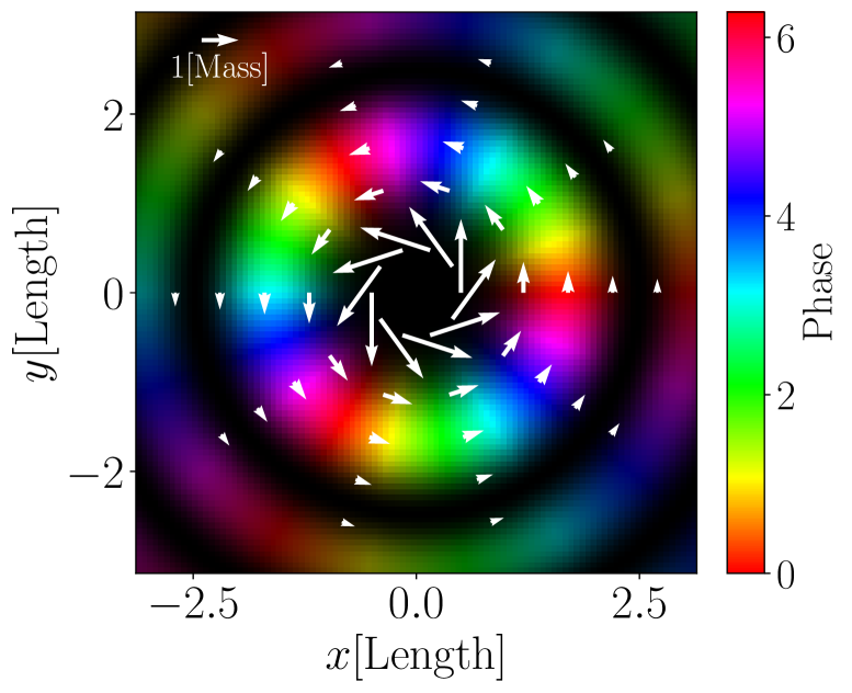
Figure 1: The transverse distribution of the wavefunction at $z=0$ and the distribution of azimuthal momentum flow in vortex particles. The white arrows indicate the local momentum in the azimuthal direction $\mathbf{p}_{\phi}(\mathbf{r})$. In the figure, the color hue represents the phase, while the brightness denotes the relative probability density.

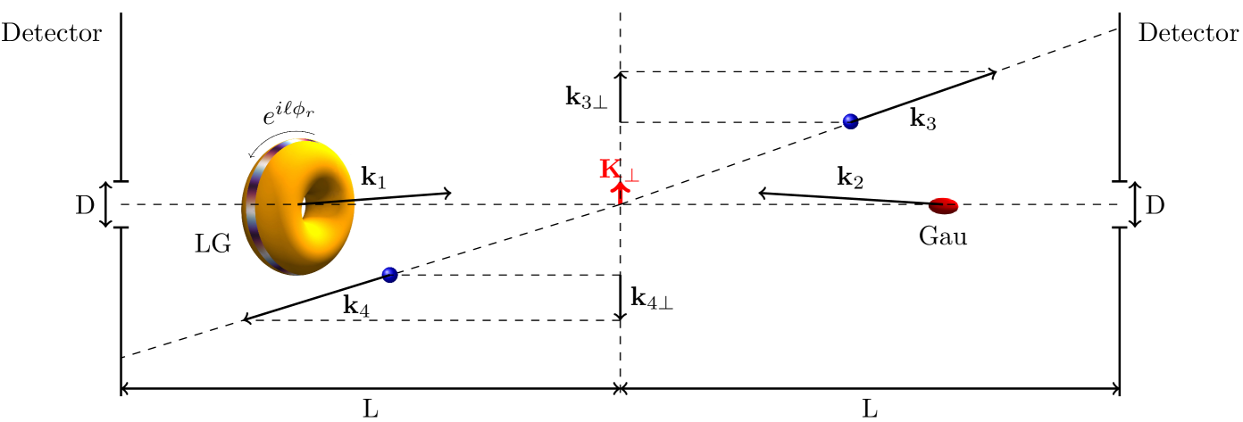
Figure 2: Schematic diagram of the experimental detection. Here, LG denotes Laguerre-Gaussian vortex electrons, and Gau represents tightly focused Gaussian wave-packet electrons. Detectors are placed at a distance $L$ on either side of the collision point to detect final-state scattered particles. Each detector has a small hole $D$ at its center to allow the passage of incident particles. $\mathbf{k}_{1}$ and $\mathbf{k}_{2}$ denote the typical plane wave components of the LG and Gaussian wave packets, respectively. $\mathbf{k}_{3}$ and $\mathbf{k}_{4}$ denote the scattered plane wave electrons.

In the wave function of a vortex particle, the vortex phase $e^{i\ell\phi_{r}}$ induces a localized component of transverse momentum, $\mathbf{p}_{\phi}(\mathbf{r})=\mathbf{j}_{\phi}(\mathbf{r})/\absolutevalue{\psi(\mathbf{r})}^{2}=\mathbf{e}_{\phi}\,\ell/r$, in the azimuthal directionBerry (2013). In Fig. 1, we illustrate a scalar particle in a Bessel vortex state as an example, showing the distribution of its probability density and local transverse momentum flow. From a semiclassical perspective, positioning a point-like test particle in the vicinity of the vortex axis induces a transverse momentum transfer exceeding the typical value carried by the vortex particle. This surprisingly large momentum transfer was dubbed the "superkick"Barnett and Berry (2013). This situation leads to a paradox: the momentum absorbed by the point-like probe particle can be much greater than the actual momentum of the vortex particle, resulting in a violation of momentum conservationBarnett and Berry (2013). To resolve this paradox, Ref. Barnett and Berry (2013); Ivanov et al. (2022) suggested that both the vortex particle and the probe particle should be described within the quantum framework. Hence, all initial states are represented as wave packets and the total energy-momentum conservation law is imposed as shown in Eq. (1). Each plane-wave component of the wave packet obeys the law of momentum conservation.

This highly localized momentum of a vortex particle can be probed via elastic scattering with normal particles of compact wave packets. As shown in Li et al. (2024), elastic scattering between vortex and ordinary electrons is proposed to reveal this effect. A detailed setup is illustrated in Fig. 2. Here a tightly focused Gaussian electron wave packet collides with a vortex electron with a non-zero impact parameter. The superkick effect manifests as follows: For an initially tightly focused Gaussian electron wave packet, the mean transverse momentum $\langle k_{y}\rangle$ is zero. However the localized transverse momentum $K_{y}$ of the vortex electron can induce an offset in the center of distribution of the superposed momentum for both scattered particles $k_{3y}+k_{4y}=K_{y}$. Furthermore, as dictated by the direction of the local transverse momentum, the offset direction is oriented perpendicular to the impact parameter $\mathbf{b}$. The momentum distribution of final electrons can be observed by detectors arranged off-axis relative to the collinear orientation, allowing the overall momentum shift to be identified, thereby revealing the vortex phase structure.

III Theoretical and Numerical Methods

In Møller scattering, when the initial-state electrons are not plane waves but possess a wave packet distribution, the S-matrix element is given by:

$$S_{fi}=\int\frac{\differential^{3}\mathbf{k}_{1}}{(2\pi)^{3}2E_{k_{1}}}\frac{\differential^{3}\mathbf{k}_{2}}{(2\pi)^{3}2E_{k_{2}}}\phi_{1}(\mathbf{k}_{1})\phi_{2}(\mathbf{k}_{2})(2\pi)^{4}\delta^{4}(k_{1}+k_{2}-K_{f})\mathcal{M}(\mathbf{k}_{1},\mathbf{k}_{2};\mathbf{k}_{3},\mathbf{k}_{4}),$$ (1)

where $\mathbf{k}_{1}$ and $\mathbf{k}_{2}$ denote the momenta of the incident electrons, while $\mathbf{k}_{3}$ and $\mathbf{k}_{4}$ denote those of the scattered electrons. The total four-momentum of the final-state particles is given by $K^{\mu}_{f}=k_{3}^{\mu}+k_{4}^{\mu}$. $\phi_{1}(\mathbf{k}_{1})$ and $\phi_{2}(\mathbf{k}_{2})$ represent the momentum distributions of the incident particle wave packets and are normalized as

$$\int\frac{\differential^{3}\mathbf{k}}{(2\pi)^{3}2E_{\mathbf{k}}}\absolutevalue{\phi_{i}(\mathbf{k})}^{2}=1.$$ (2)

In Eq. (1), $\mathcal{M}$ denotes the invariant matrix element associated with the process under consideration. In our calculation, this corresponds to the invariant matrix element for Møller scattering, whose explicit form is given in Refs. Greiner and Reinhardt (2008); Berestetskii et al. (1982).

III.1 Numerical Method

In numerical calculations, explicit accounting for the specific forms of the wave packet $\phi_{i}(\mathbf{k})$ and the invariant matrix element $\mathcal{M}$ is not required. By exploiting the properties of the delta function, the six-fold integral in Eq. (1) can be reduced to a two-fold integral, yielding the following expression:

$$S_{fi}=\int\frac{\sqrt{E_{k_{1}}^{2}-m_{e}^{2}}\differential\Omega_{k_{1}}}{(2\pi)^{2}4E_{k_{2}}}\phi(\mathbf{k}_{1})\phi(\mathbf{k}_{2})\frac{1}{4\Delta}\mathcal{M}(\mathbf{k}_{1},\mathbf{k}_{2};\mathbf{k}_{3},\mathbf{k}_{4}),$$ (3)

where $\mathbf{k}_{2}=\mathbf{K}_{f}-\mathbf{k}_{1}$ and $E_{k_{2}}=E_{f}-E_{k_{1}}$. In Eq. (3), the $\Delta$ factor and the energy $E_{k_{1}}$ are given by

$$\Delta=\sqrt{K_{f}^{2}\cos^{2}\theta(E_{f}^{4}+K_{f}^{4}-2E_{f}^{2}(2m^{2}+K_{f}^{2})+4m^{2}K_{f}^{2}\cos^{2}\theta)}$$ (4)

and

$$E_{k_{1}}=\frac{E_{f}(E_{f}^{2}-P_{f}^{2})+\Delta}{2(E_{f}^{2}-P_{f}^{2}\cos^{2}\theta)},$$ (5)

with $\theta$ denoting the angle between $\mathbf{K}_{f}$ and $\mathbf{k}_{1}$. For Eq. (3), numerical methods such as the Newton-Cotes formulas or the trapezoidal rule can be used for computation Scherer and Scherer (2017).

The calculation of the differential probability requires six-dimensional phase-space integration

$$\differential W=\absolutevalue{S_{fi}}^{2}\frac{\differential^{3}\mathbf{k}_{3}}{(2\pi)^{3}2E_{k_{3}}}\frac{\differential^{3}\mathbf{k}_{4}}{(2\pi)^{3}2E_{k_{4}}}.$$ (6)

The Monte Carlo integration method Lepage (2021) was employed to efficiently compute the differential scattering probability.

III.2 Analytical Model-Relativistic Regime and Paraxial Approximation

We employ the Laguerre-Gaussian (LG) wave packet and the Gaussian wave packet to describe initial-state electrons $\phi_{1}$ and $\phi_{2}$, respectively

$$\phi_{1}(\mathbf{k}_{1})\propto\frac{(\sigma_{1\perp}k_{1\perp})^{\ell}}{\sqrt{\ell!}}\exp[-\frac{k_{1\perp}^{2}\sigma_{1\perp}^{2}}{2}-\frac{(k_{1z}-p_{1z})^{2}\sigma^{2}_{1z}}{2}+i\ell\phi_{k_{1}}],$$ (7)

$$\phi_{1}(\mathbf{k}_{2})\propto\exp[-\frac{k_{2\perp}^{2}\sigma_{2\perp}^{2}}{2}-\frac{(k_{2z}-p_{2z})^{2}\sigma^{2}_{2z}}{2}+i\mathbf{b}_{\perp}\cdot\mathbf{k}_{2\perp}].$$ (8)

We assume that the transverse ($\sigma_{1\perp}$ and $\sigma_{2\perp}$) and longitudinal dimensions ($\sigma_{1z}$ and $\sigma_{2z}$) of the wave packets are on the nanometer scale Karlovets and Serbo (2020), and the corresponding momentum broadening is on the order of hundreds of electron volts. We adopt the central momenta of the incident particles as $p_{1z}=10$MeV and $p_{2z}=-10$MeV, much larger than the momentum spread of the wave packets $p_{zi}\sigma_{zi}\gg 1$. In this case, the incident particles are in the strongly paraxial regime, with the divergence angles of the wave packets given by $k_{1\perp}/k_{1z}\sim k_{2\perp}/k_{2z}\sim 10^{-5}$.

For final-state scattered electrons, the cross section in Møller scattering is proportional to $1/\sin^{4}\theta$ Greiner and Reinhardt (2008); Berestetskii et al. (1982). As a result, the majority of the scattering signal is concentrated in the paraxial region. To effectively separate the scattered electron signal from the background, we analyze electrons scattered at angles in the range of 1–5 mrad. This corresponds to a transverse momentum of approximately 10 keV, which exceeds the transverse momenta of both the initial LG and Gaussian wave packets, $k_{1\perp}$ and $k_{2\perp}$, even when considering their broadening.

In the Born approximation, the amplitude of Møller scattering is given byGreiner and Reinhardt (2008); Berestetskii et al. (1982)

$$\mathcal{M}\propto\biggl{(}\frac{\bar{u}_{k_{3}}\gamma^{\mu}u_{k_{1}}\bar{u}_{k_{4}}\gamma_{\mu}u_{k_{2}}}{t}-\frac{\bar{u}_{k_{4}}\gamma^{\mu}u_{k_{1}}\bar{u}_{k_{3}}\gamma_{\mu}u_{k_{2}}}{u}\biggr{)}.$$ (9)

In the paraxial scattering regime ($\theta\ll 1$), the t-channel contribution, proportional to $1/(1-\cos\theta)$, significantly higher than that of the u-channel of $1/(1+\cos\theta)$. Therefore, we consider only the former. In the paraxial and relativistic regime, we evaluate the electron bispinor $u_{k_{i}}$ in the limit $\theta_{k_{i}}\rightarrow 0$, where $i=1,2,3,4$, and neglect the electron massLi et al. (2024). Then the amplitude in Eq .(9) scales as $\mathcal{M}\propto 1/t$. The Mandelstam variable $t$ can be simplified to

$$t=(k_{3}-k_{1})^{2}\approx-(\mathbf{k}_{1\perp}-\mathbf{k}_{3\perp})^{2}.$$ (10)

With $k_{3\perp}\gg k_{1\perp}$, the term $1/(\mathbf{k}_{1\perp}-\mathbf{k}_{3\perp})^{2}$ is expanded:

$$\frac{1}{(\mathbf{k}_{1\perp}-\mathbf{k}_{3\perp})^{2}}\approx\frac{1}{k^{2}_{3\perp}}\biggl{[}1+2\frac{k_{1\perp}}{k_{3}{\perp}}\cos(\phi_{k_{3}}-\phi_{k_{1}})\biggr{]}.$$ (11)

The invariant amplitude can be approximated accordingly

$$\mathcal{M}\propto\frac{1}{k^{2}_{3\perp}}\biggl{[}1+2\frac{k_{1\perp}}{k_{3}{\perp}}\cos(\phi_{k_{3}}-\phi_{k_{1}})\biggr{]}\delta_{\lambda_{1}\lambda_{3}}\delta_{\lambda_{2}\lambda_{4}}.$$ (12)

The Kronecker $\delta$ in Eq. (12) indicates that helicities are always conserved along each fermion line. As stated in Ref. Liu and Ivanov (2023), the differential probability is thus derived

$$\differential W\propto\absolutevalue{\mathcal{I}_{\perp}}^{2}\differential^{2}\mathbf{k}_{\perp 3}\differential^{2}\mathbf{K}_{f\perp},$$ (13)

where

$$\mathcal{I}_{\perp}\propto\, i^{\ell}\sigma_{1\perp}^{\ell}e^{-\frac{K_{f\perp}^{2}\sigma_{2\perp}^{2}}{2}}e^{i\ell\phi_{B}}\frac{1}{k_{3\perp}^{2}}$$

$$\biggl{(}N_{\ell+1,\ell}+\frac{1}{k_{3\perp}}i^{-1}e^{-i\phi_{B}}e^{i\phi_{k_{3}}}N_{\ell+2,\ell-1}+\frac{1}{k_{3\perp}}ie^{i\phi_{B}}e^{-i\phi_{k_{3}}}N_{\ell+2,\ell+1}\biggr{)}.$$ (14)

In Eq. (14), $N_{m,n}$ is defined by the Whittaker function Gradshteyn and Ryzhik (2014)

$$N_{m,n}(\alpha,\beta)\equiv\frac{\Gamma(m/2+n/2+1/2)}{\beta\alpha^{m/2}\Gamma(n+1)}\exp(-\frac{\beta^{2}}{8\alpha})M_{m/2,n/2}\biggl{(}\frac{\beta^{2}}{4\alpha}\biggr{)}$$ (15)

and

$$\phi_{B}=\arctan(\frac{b_{y}-iK_{fy}\sigma_{2\perp}^{2}}{b_{x}-iK_{fx}\sigma_{2\perp}^{2}}).$$ (16)

III.3 Benchmark

The results from numerical methods and analytical approximations are benchmarked considering a total angular momentum of 11/2 for the vortex-state electron. The incident LG wave packet has a transverse width of $\sigma_{1\perp}$=10nm and a longitudinal width of $\sigma_{1z}$=5nm, while the Gaussian wave packet has $\sigma_{2\perp}$=2nm and $\sigma_{2z}$=1nm.

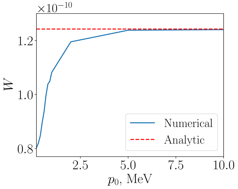
Figure 3: The total probability $W$ as a function of the incident electron momentum $p_{0}$. The impact parameters are set to $b_{x}=20$nm and $b_{y}=0$nm. The term ’Numerical’ refers to results obtained from the numerical method, while ’Analytic’ denotes results derived under the relativistic paraxial approximation. The integration range of $k_{3\perp}$ is fixed from 10 keV to 50 keV.

Fig. (3) compares the probability from both methods at different incident electron momentum $p_{0}$. When the electron momentum is significantly larger than its rest mass ($p_{0}>5$MeV), the analytical results match the numerical one perfectly, as clearly demonstrated by Eqs. (13) and (14). However, in the weakly relativistic regime, while the analytical value remains constant, the numerical one declines significantly, suggesting that the approximation is no longer applicable. Thus, when considering experimental validation using weakly relativistic electrons, such as those from a transmission electron microscope (TEM), we rely on the numerical method for evaluation. Here although the overall probability decreases the superkick effect remains observable.

IV Impact of Various Factors

The superkick effect manifests itself in the differential scattering probability as a function of the total transverse momentum $\mathbf{K}_{f}$ of the final-state particles

$$w(\mathbf{K}_{f\perp})=\frac{\differential W}{\differential^{2}\mathbf{K}_{f\perp}}=\int\absolutevalue{S_{fi}}^{2}\frac{\differential^{3}\mathbf{k}_{3}\differential k_{4z}}{(2\pi)^{6}4E_{k_{3}}E_{k_{4}}}.$$ (17)

Fig. 4 presents the detailed results using the parameters from Fig. 3. The total transverse momentum exhibits a noticeable displacement perpendicular to $b_{x}$. This shift vanishes if one removes the vortex phase in the momentum space of the LG wave packet (Fig. 4(b) ) or in the coordinate space (4(c)) .

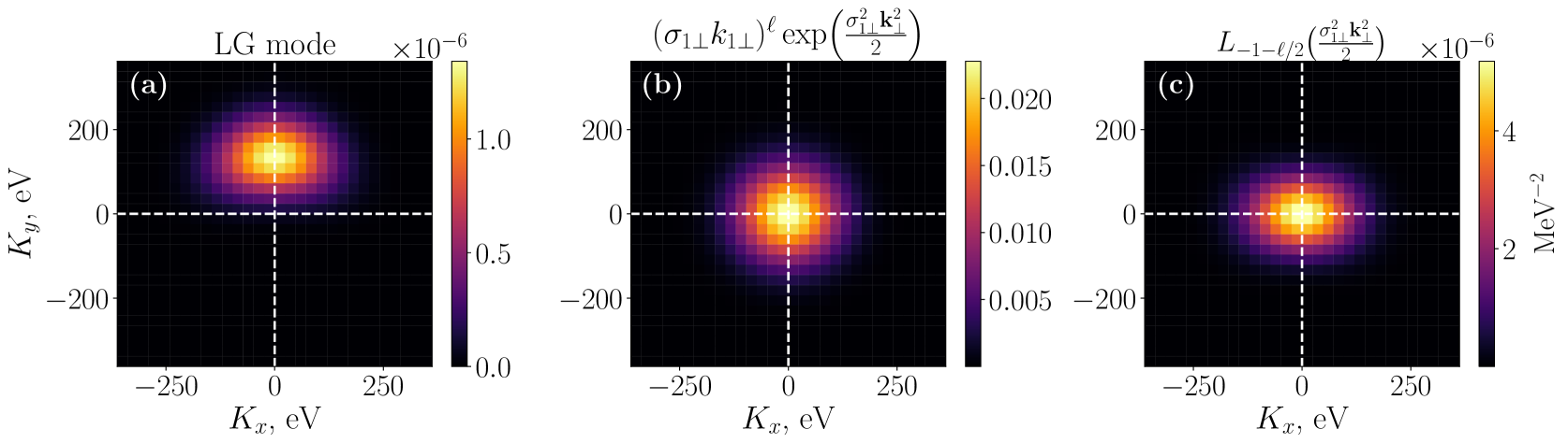
Figure 4: The total transverse momentum distribution is shown, with the collision parameter $\mathbf{b}$ fixed at $b_{x}=5$nm and $b_{y}=0$nm for panels (a) through (c). The incident electron energy is 10 MeV. The transverse momentum distribution of the wave packet is specified in the title of each subfigure.

Figure 5: (a): Average transverse momentum $\langle K_{y}\rangle$ as a function of the impact parameter $b_{x}$. The black dashed line, $\sqrt{\ell}/\sigma_{1\perp}$, represents the characteristic transverse momentum of the LG vortex electron. The orange dashed line corresponds to the local transverse momentum, $\frac{\ell}{b}\mathbf{e}_{y}$, induced by the vortex phase. (b): Scattering probability as a function of the impact parameter $b_{x}$.

Fig. 5(a) shows the expectation value of the transverse momentum $\langle K_{y}\rangle$ of the scattered particles as a function of the impact parameter $b_{x}$. For small values of $b_{x}$, the average transverse momentum $\langle K_{y}\rangle$ goes beyond the characteristic transverse momentum of the vortex particles, $\sqrt{\ell}/\sigma_{1\perp}$. In semiclassical picture, the momentum diverge at center. However, in the quantum picture, it converges to 0 at $b_{x}=0$. This effect arises due to the wave packet nature of the probe particle. When a finite-sized wave packet approaches the phase singularity, it encounters symmetric transverse momenta from various azimuthal directions, which cancel each other out, thus preventing the divergence of $\ell/b$. As the impact parameter $b_{x}$ increases, $\langle K_{y}\rangle$ gradually approaches $\ell/b$, in agreement with the momentum transfer predicted by the semiclassical picture.

In Fig. 5(b), we present the scattering probability for different impact parameters. One may ask how momentum is conserved when superkick happens. This phenomenon arises due to the localized tangential momentum of vortex phase structure. Although $\langle K_{y}\rangle$ exceeds the transverse momentum $\sqrt{\ell}/\sigma_{1\perp}$ for small impact radii, it gradually drops below this value as $b$ increases. In other words, it is a redistribution of momentum induced by the localized kick. By weighting $\langle K_{y}\rangle$ with the scattering probability $W$ and integrating over $b$, we obtain the average transverse momentum $\bar{K}_{y}=\int\langle K_{y}\rangle W\differential b/\int W\differential b$. This corresponds to the red dashed line in Fig. 5(a). We observe that $\bar{K}_{y}$ exactly matches the characteristic transverse momentum of the vortex particle, i.e., momentum is conserved averagely in this process.

The comparison in Fig. 4 is straightforward. However, in more realistic scenarios, it is essential to account for various factors that have non-negligible effects on the results, including the alignment jitter of electron sources, collisions at non-collinear geometries, the finite size of wave packets and other related considerations. We therefore conduct a systematic analysis of these factors to provide guidance for future experiments. Unless explicitly stated otherwise, the main parameters follow those in Fig. 4.

IV.1 Effects of Alignment Jitter and Statistics

In realistic experiments, it is impossible to precisely control the impact parameter of two colliding electron beams, as alignment jitter is always present, especially when signals are collected from an adequate number of scattering events.

Figure 6: (a): The average transverse momentum $\langle K_{y}\rangle$ is shown as a function of the impact parameter $b_{0}$ for different fluctuation amplitudes $\sigma_{b}$. (b): The number of scattered particles varies as a function of the impact parameter $b_{0}$. (c): The statistical significance of a non-zero $\langle K_{y}\rangle$ is analyzed as a function of the impact parameter $b_{0}$. The transverse size of the Gaussian wave packet is $\sigma_{2\perp}=2$nm. The collision parameters are defined as $b_{x}=b_{0}$ and $b_{y}=0$.

The jitter is modeled using the following distribution:

$$f(\mathbf{b};\mathbf{b}_{0})=\frac{1}{\pi\sigma_{b}^{2}}\exp[-\frac{(\mathbf{b}-\mathbf{b}_{0})^{2}}{\sigma_{b}^{2}}],$$ (18)

where $\mathbf{b}_{0}$ is the center of the distribution and $\sigma_{b}$ represents its characteristic width. After accounting for the distribution, the smeared differential probability $\bar{w}(\mathbf{K}_{\perp})$ is defined as:

$$\bar{w}(\mathbf{K}_{\perp};\mathbf{b}_{0})=\int w(\mathbf{K}_{\perp};\mathbf{b})f(\mathbf{b};\mathbf{b}_{0})\differential^{2}\mathbf{b}.$$ (19)

The distribution of the averaged transverse momentum $\langle K_{y}\rangle$ as a function of $b_{0}$ of the jitter radii $\sigma_{b}$ is shown in Fig.6(a). Apparently, the superkick effect gradually diminishes as the jitter becomes more significant.

In this scheme, the interactions between electrons within each electron beam should be neglected. Therefore, it is required that spacing among the electrons is larger than the size of electron wave packets. For instance, with an average current of 16 nA electron source, their average spacing is about 3 mm, sufficiently large as compared to the wave packet size. An experiment running for $10^{3}$ seconds yields $N_{0}=10^{14}$ electron collision attempts. As shown in Fig. 6(b), approximately $10^{4}$ scattered electron signals around $b\approx\sigma_{1\perp}$ are expected. The detector response ($5\times 10^{6}$ electrons per pixel per second) Dijkstra (2002); Dubey et al. (2024) is sufficient for our purpose.

As illustrated in Fig. 5, the total transverse momentum shows a deviation of 150 eV. This naturally raises the question of how well such a small momentum shift can be resolved in an electron beam of 10 MeV. Importantly, we do not directly measure the tiny momentum shift. Instead, the transverse momenta of the scattered particles, $k_{3\perp}$ and $k_{4\perp}$, whose magnitudes are on the order of 10 keV, are recorded. This is well within the range of realistic experimental detectors. By simultaneously measuring both $k_{3\perp}$ and $k_{4\perp}$, we can determine the total transverse momentum $K_{\perp}=k_{3\perp}+k_{4\perp}$.

In addition, when detecting final-state particles, their momentum cannot be precisely determined. Therefore, consideration of the transverse momentum uncertainty is essential. Here, we set $L$ and $D$ to 2m and 4mm, respectively, as shown in the experimental schematic in Fig. 2. In the experimental proposal, we consider using a pixelated silicon (Si) electron detector Dijkstra (2002); Dubey et al. (2024), which offers resolution of 70 $\mu$m with each pixel. This corresponds to a transverse momentum uncertainty of $\delta k_{\perp}=350$ eV for detecting the scattered electrons.

Taking into account alignment jitter, signal statistics, and the finite momentum resolution in the detection of final-state particles, we define the statistical significance $S$

$$S=\frac{\langle K_{y}\rangle\sqrt{N(b_{0})}}{\sqrt{\langle K_{y}^{2}\rangle+(\delta k_{\perp})^{2}}},$$ (20)

to evaluate the outcome. The effect is deemed experimentally observable when the statistical significance $S$ is greater than 5. As shown in Fig. 6(c), although the superkick effect is strong at smaller values of $b$, the limited number of scattering signals poses a challenge for experimental detection, leading to a lower statistical significance. Taking into account all relevant factors, the optimal impact position is $b\sim\sqrt{\ell}\sigma_{1\perp}$, which maximizes statistical significance. Furthermore, we find that even if the position uncertainty $\sigma_{b}$ is comparable to the transverse size of the LG wave packet $\sigma_{1\perp}$, a nonzero $\langle K_{y}\rangle$ can still be experimentally observed.

IV.2 Effects of Non-collinear Collision

Figure 7: Schematic of a non-collinear collision setup, where the crossing angle $\theta$ is defined

As shown in Fig. 7, in a more realistic experimental setup, in order to separate the two beamlines, the collisions can be arranged at an appropriate nonzero crossing angle. The distribution of the differential scattering probability $w(\mathbf{K}_{\perp})$ for a crossing angle of $\pi/4$ has been obtained, as illustrated in Fig. (8)(a).

Figure 8: (a):Distribution of $w(\mathbf{K}_{\perp})$ at a crossing angle of 45 degrees. (b): Distribution of $w(\mathbf{K}_{\perp})$ at the collision of two Gaussian wave packets for the same crossing angle. In both cases, the collision parameters are set as $b_{x}=5$nm and $b_{y}=0$nm. The horizontal axis has been offset by subtracting the momentum change in the x-direction due to a cross collision, given by $k_{0x}=k_{0}\sin(3\pi/4)\approx 7.07$ MeV.

The center of the total transverse momentum $K_{x}$ shifts from 0 to $k_{0x}=k_{0}\sin(3\pi/4)\approx 7.07$ MeV due to the cross collision. In contrast, the shift along the $K_{y}$-direction is evident due to the superkick effect. For comparison, we analyzed the collision between two Gaussian wave packets at the same crossing angle, as shown in Fig. (8)(b). In this case, the displacement of the distribution center along the $K_{y}$-direction vanishes.

We further examine the effect of the crossing angle $\theta$, and the results are presented in Fig. 9.

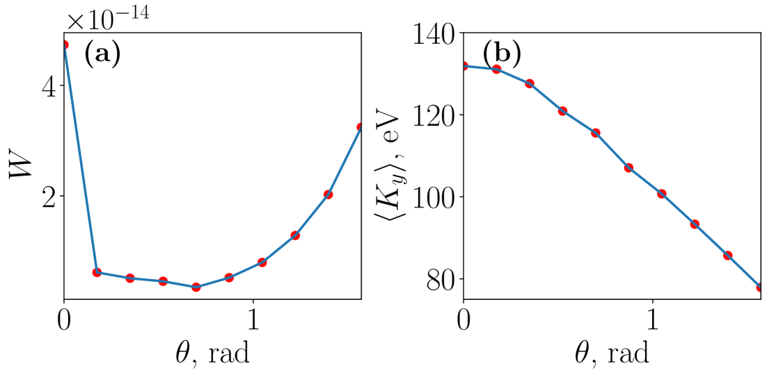
Figure 9: The scattering probability (a) and the averaged total transverse momentum $\langle K_{y}\rangle$ (b) are analyzed as a function of the crossing angle under non-collinear collisions. We set the impact parameters to $b_{x}=5$nm and $b_{y}=0$nm.

Fig. 9(a) shows that as the crossing angle increases, the scattering probability declines and then gradually rises up. This is because in non-collinear collisions the wave packets overlap for a shorter duration at a small crossing angles. When the crossing angle further increases, the tightly focused Gaussian wave packet passes through both sides of the ’ring’ of the LG vortex particle, where its probability density peaks. However, the superkick effect, denoted by $\langle K_{y}\rangle$, decreases as the angle increases. In non-collinear collisions, the trajectory of the probe crosses a line related to varying impact parameters, thus the local transverse momentum shall be averaged, which leads to lower values at larger angles.

IV.3 Effects of the Wave Packet Size of the Gaussian Probe

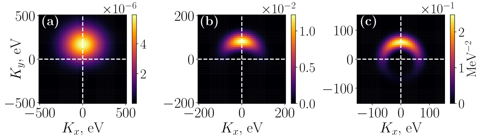
Figure 10: (a)-(c):The Gaussian wave packets have transverse sizes of 1, 5, and 10 nm respectively. The impact parameters are $b_{x}=$5 nm and $b_{y}=$0 nm.

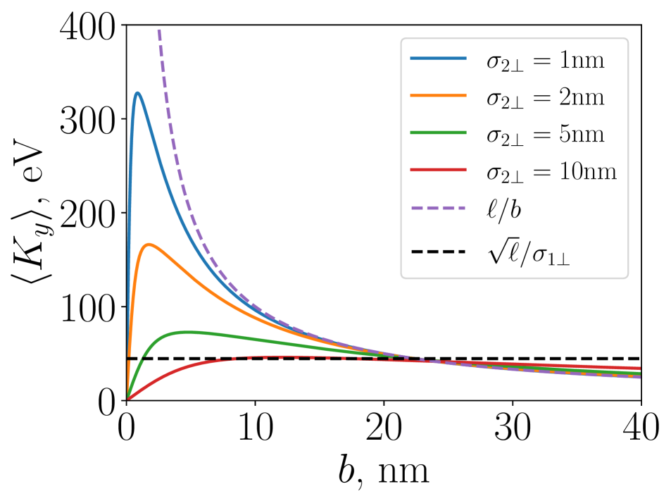
Figure 11: Effect of different transverse sizes of Gaussian wave packets on the average transverse momentum.

In general, the superkick effect is more significant when the probe is more localized. Fig. 10 presents the differential scattering probability by changing transverse sizes of Gaussian wave packets, following

$$w(\mathbf{K}_{f\perp})=\frac{\differential W}{\differential^{2}\mathbf{K}_{f\perp}}=\int\absolutevalue{S_{fi}}^{2}\frac{\differential^{3}\mathbf{k}_{3}\differential k_{4z}}{(2\pi)^{6}4E_{k_{3}}E_{k_{4}}}.$$ (21)

The momentum displacements are centered around 200, 100, and 50 eV in 10(a), 10(b), and 10(c), for wave packet sizes of 1, 5 and 10 nm, respectively. As the Gaussian wave packet size is approaching to the LG one, the distribution exhibits annular shape, a reflection of the vortex intensity profile.

The above trend is clearly seen in the $b_{x}$-dependent distribution in Fig. 11. When the transverse size of the Gaussian wave packet is set to $\sigma_{2\perp}=\sigma_{1\perp}=10$nm, the total mean transverse momentum is slightly below the characteristic value $\sqrt{\ell}/\sigma_{1\perp}$ of the LG vortex; hence, the superkick effect disappears.

IV.4 The Azimuth Distribution of the Scattered Particles

In addition to the total transverse momentum distribution of final-state particles, we further consider the angular distribution of one of the scattered particles, $k_{3}$. This dependence can also be found in Eq. (12) and Eq.(14) . The distribution is defined as follows:

$$\Phi(\phi_{k_{3}})=\frac{\differential W}{\differential\phi_{k_{3}}}=\int\absolutevalue{S_{fi}}^{2}\frac{k_{3\perp}\differential k_{3\perp}\differential k_{3z}\differential^{3}\mathbf{k}_{4}}{(2\pi)^{6}4E_{k_{3}}E_{k_{4}}}.$$ (22)

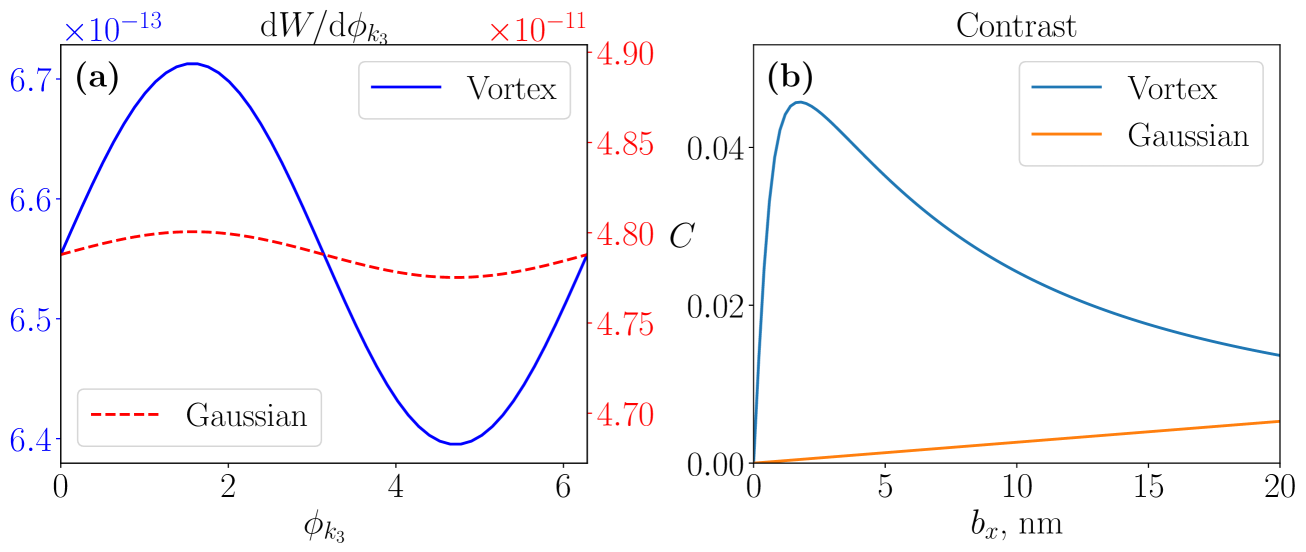
Figure 12: (a): The distribution of the differential scattering probability with respect to the azimuthal angle $\phi_{k_{3}}$ of the scattered electron. the impact parameters are set to $b_{x}=10$nm and $b_{y}=0$nm. Vortex particle scattering is represented by the left vertical axis, while Gaussian wave packet scattering is represented by the right vertical axis. (b): Dependence of the contrast C on the impact parameter $b_{x}$.

Fig. 12(a) shows that for a nonzero impact parameter, the azimuthal distribution of the final-state electron follows a sinusoidal pattern. It appears for both Gaussian wave packet collisions and vortex scattering but more pronounced in the latter. To characterize this phenomenon, we define the contrast $C$ of the distribution to calibrate the degree of variation

$$C=\frac{\Phi_{\text{max}}-\Phi_{\text{min}}}{\Phi_{\text{max}}+\Phi_{\text{min}}}.$$ (23)

In Fig. 12(b), while the contrast is zero at $b_{x}=0$nm in both cases, we find that the one in vortex scattering is greater by an order of magnitude than that in Gaussian scattering. Further, a peak appears around $b\sim 2$ nm for vortex scattering. The distinctive trend in azimuth distribution provides an additional approach to identify the superkick effect.

IV.5 The Spin Flip Effect

It is also of interest to determine whether spin flip plays a significant role in this process. Eq. (1) shows that the superkick effect originates from the vortex phase of the wave packet, whereas spin flip originates from the invariant amplitude $\mathcal{M}$, with no direct coupling between them.

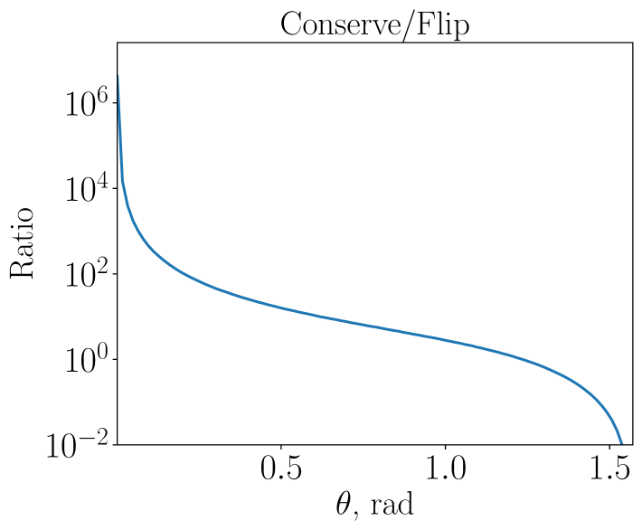
Figure 13: The ratio of the differential scattering probabilities of spin-conserving to spin-flip as a function of $\theta_{k_{3}}$. In the figure, the azimuthal angle is fixed at $\pi/2$.

Owing to the nature of Møller scattering, most of the scattered electrons remain in the paraxial region. In this region, spin-flip transitions are significantly suppressed. According to QED theory, spin conservation prevails over spin flip by a factor of $1/\theta^{2}$. In the Fig. 13, we present the ratio of the differential scattering probability for spin-conserving to that for spin-flip as a function of the polar angle $\theta_{k_{3}}$ of the scattered electron.. As shown in Fig. 13, in the paraxial region, the spin-conserving channel dominates over the spin-flip channel by six orders of magnitudes. Beyond the paraxial region, the spin-flip effect becomes more obvious. For large scattering angles ($\theta_{k_{3}}\geq 1.2$), the spin-conserving channel is significantly suppressed, allowing the spin-flip channel to dominate.

V Conclusions and Perspectives

Vortex particle scattering offers a unique degree of freedom for advancing our understanding of atomic, nuclear, and particle physics. The detection of high-energy vortex particles is a crucial step in such studies. To tackle this problem, we propose an experimental scheme based on the superkick effect that enables the characterization of the vortex properties of vortex particles Li et al. (2024).

In this work, we present a detailed analysis of the proposed scheme. We provided both exact numerical calculations and analytical expressions under the relativistic paraxial approximation and investigated several factors that could potentially affect the detection efficiency, among which the transverse size of the wave packets and alignment jitter plays important roles. Effects such as spin flip and the energy of the incident electron have a minor influence on the superkick effect. We also pointed out that the superkick effect can still be observed in more realistic situations such as non-collinear collision configuration.

Furthermore, we demonstrated that the vortex phase also manifests as an asymmetry in the azimuthal distribution of a single scattered electron. Employing a single-particle detection method relaxes the stringent requirement on detector response time.

While our calculations in this paper are illustrated using Møller scattering, the superkick effect is a ubiquitous feature of various vortex scattering processes, including Compton scattering and electron-proton scattering. Extending this idea to the detection of high-energy vortex states of photons, ions, and hadrons is a natural progression, a topic that will be explored in more detail in future work.

VI Acknowledgments

S.L. thanks Yujian Lin for his assistance with Fig. 2. S.L. and L.J. thank Sun Yat-sen University for hospitality during the workshop ’Vortex states in nuclear and particle physics’. S.L. and L.J. acknowledge the support by National Science Foundation of China (Grant No. 12388102), CAS Project for Young Scientists in Basic Research (Grant No. YSBR060), and the National Key R&D Program of China (Grant No. 2022YFE0204800). B.L. and I.P.I. thank the Shanghai Institute of Optics and Fine Mechanics for hospitality during their visit.

References

- Allen et al. (1992) L. Allen, M. W. Beijersbergen, R. Spreeuw, and J. Woerdman, Physical review A 45, 8185 (1992).
- Bliokh et al. (2007) K. Y. Bliokh, Y. P. Bliokh, S. Savel’Ev, and F. Nori, Physical Review Letters 99, 190404 (2007).
- Uchida and Tonomura (2010) M. Uchida and A. Tonomura, nature 464, 737 (2010).
- Verbeeck et al. (2010) J. Verbeeck, H. Tian, and P. Schattschneider, Nature 467, 301 (2010).
- Lee et al. (2019) J. T. Lee, S. Alexander, S. Kevan, S. Roy, and B. McMorran, Nature Photonics 13, 205 (2019).
- Sarenac et al. (2022) D. Sarenac, M. E. Henderson, H. Ekinci, C. W. Clark, D. G. Cory, L. DeBeer-Schmitt, M. G. Huber, C. Kapahi, and D. A. Pushin, Science Advances 8, eadd2002 (2022).
- Luski et al. (2021) A. Luski, Y. Segev, R. David, O. Bitton, H. Nadler, A. R. Barnea, A. Gorlach, O. Cheshnovsky, I. Kaminer, and E. Narevicius, Science 373, 1105 (2021).
- Bliokh et al. (2017) K. Y. Bliokh, I. P. Ivanov, G. Guzzinati, L. Clark, R. Van Boxem, A. Béché, R. Juchtmans, M. A. Alonso, P. Schattschneider, F. Nori, et al., Physics Reports 690, 1 (2017).
- Ivanov (2022) I. P. Ivanov, Progress in Particle and Nuclear Physics 127, 103987 (2022).
- Afanasev et al. (2013) A. Afanasev, C. E. Carlson, and A. Mukherjee, Physical Review A—Atomic, Molecular, and Optical Physics 88, 033841 (2013).
- Scholz-Marggraf et al. (2014) H. Scholz-Marggraf, S. Fritzsche, V. Serbo, A. Afanasev, and A. Surzhykov, Physical Review A 90, 013425 (2014).
- Zadernovsky (2006) A. Zadernovsky, Laser physics 16, 571 (2006).
- Wu et al. (2022) Y. Wu, S. Gargiulo, F. Carbone, C. H. Keitel, and A. Pálffy, Physical Review Letters 128, 162501 (2022).
- Afanasev and Carlson (2022) A. Afanasev and C. E. Carlson, Annalen der Physik 534, 2100228 (2022).
- Jentschura and Serbo (2011a) U. D. Jentschura and V. G. Serbo, Physical Review Letters 106, 013001 (2011a).
- Jentschura and Serbo (2011b) U. D. Jentschura and V. G. Serbo, The European Physical Journal C 71, 1 (2011b).
- Taira et al. (2017) Y. Taira, T. Hayakawa, and M. Katoh, Scientific reports 7, 5018 (2017).
- Chen et al. (2019) Y.-Y. Chen, K. Z. Hatsagortsyan, and C. H. Keitel, Matter and Radiation at Extremes 4 (2019).
- Ababekri et al. (2024) M. Ababekri, R.-T. Guo, F. Wan, B. Qiao, Z. Li, C. Lv, B. Zhang, W. Zhou, Y. Gu, and J.-X. Li, Phys. Rev. D 109, 016005 (2024).
- Floettmann and Karlovets (2020) K. Floettmann and D. Karlovets, Physical Review A 102, 043517 (2020).
- Bu et al. (2024) Z. Bu, L. Ji, X. Geng, S. Liu, S. Lei, B. Shen, R. Li, and Z. Xu, Advanced Science 11, 2404564 (2024).
- Dyatlov et al. (2024) A. Dyatlov, V. Bleko, K. Cherepanov, V. Kobets, M. Martyanov, M. Nozdrin, A. Sergeev, N. Sheremet, A. Zhemchugov, and D. Karlovets, in 2024 International Conference Laser Optics (ICLO) (2024) pp. 438–438.
- zhu (2024) Workshop on Vortex states in nuclear and particle physics (Zhuhai, China, 2024).
- Saitoh et al. (2013) K. Saitoh, Y. Hasegawa, K. Hirakawa, N. Tanaka, and M. Uchida, Physical review letters 111, 074801 (2013).
- Guzzinati et al. (2014) G. Guzzinati, L. Clark, A. Béché, and J. Verbeeck, Physical Review A 89, 025803 (2014).
- Li et al. (2024) Z. Li, S. Liu, B. Liu, L. Ji, and I. P. Ivanov, Physical Review Letters 133, 265001 (2024).
- Barnett and Berry (2013) S. M. Barnett and M. Berry, Journal of Optics 15, 125701 (2013).
- Afanasev et al. (2022) A. Afanasev, C. E. Carlson, and A. Mukherjee, Physical Review A 105, L061503 (2022).
- Ivanov et al. (2022) I. P. Ivanov, B. Liu, and P. Zhang, Phys. Rev. A 105, 013522 (2022).
- Liu and Ivanov (2023) B. Liu and I. P. Ivanov, Physical Review A 107, 063110 (2023).
- Berry (2013) M. Berry, European Journal of Physics 34, 1337 (2013).
- Greiner and Reinhardt (2008) W. Greiner and J. Reinhardt, Quantum electrodynamics (Springer Science & Business Media, 2008).
- Berestetskii et al. (1982) V. B. Berestetskii, E. M. Lifshitz, and L. P. Pitaevskii, Quantum Electrodynamics: Volume 4, Vol. 4 (Butterworth-Heinemann, 1982).
- Scherer and Scherer (2017) P. O. Scherer and P. O. Scherer, Computational physics: simulation of classical and quantum systems (Springer, 2017).
- Lepage (2021) G. P. Lepage, Journal of Computational Physics 439, 110386 (2021).
- Karlovets and Serbo (2020) D. V. Karlovets and V. G. Serbo, Phys. Rev. D 101, 076009 (2020).
- Gradshteyn and Ryzhik (2014) I. S. Gradshteyn and I. M. Ryzhik, Table of integrals, series, and products (Academic press, 2014).
- Dijkstra (2002) H. Dijkstra, Nuclear Instruments and Methods in Physics Research Section A: Accelerators, Spectrometers, Detectors and Associated Equipment 478, 37 (2002).
- Dubey et al. (2024) R. Dubey, K. Czerski, M. Kaczmarski, A. Kowalska, N. Targosz-Ślęczka, M. Valat, et al., Measurement 228, 114392 (2024).