Using Powerful Prior Knowledge of Diffusion Model in Deep Unfolding Networks for Image Compressive Sensing

Abstract

Recently, Deep Unfolding Networks (DUNs) have achieved impressive reconstruction quality in the field of image Compressive Sensing (CS) by unfolding iterative optimization algorithms into neural networks. The reconstruction quality of DUNs depends on the learned prior knowledge, so introducing stronger prior knowledge can further improve reconstruction quality. On the other hand, pre-trained diffusion models contain powerful prior knowledge and have a solid theoretical foundation and strong scalability, but it requires a large number of iterative steps to achieve reconstruction. In this paper, we propose to use the powerful prior knowledge of pre-trained diffusion model in DUNs to achieve high-quality reconstruction with less steps for image CS. Specifically, we first design an iterative optimization algorithm named Diffusion Message Passing (DMP), which embeds a pre-trained diffusion model into each iteration process of DMP. Then, we deeply unfold the DMP algorithm into a neural network named DMP-DUN. The proposed DMP-DUN can use lightweight neural networks to achieve mapping from measurement data to the intermediate steps of the reverse diffusion process and directly approximate the divergence of the diffusion model, thereby further improving reconstruction efficiency. Extensive experiments show that our proposed DMP-DUN achieves state-of-the-art performance and requires at least only 2 steps to reconstruct the image. Codes are available at https://github.com/FengodChen/DMP-DUN-CVPR2025.

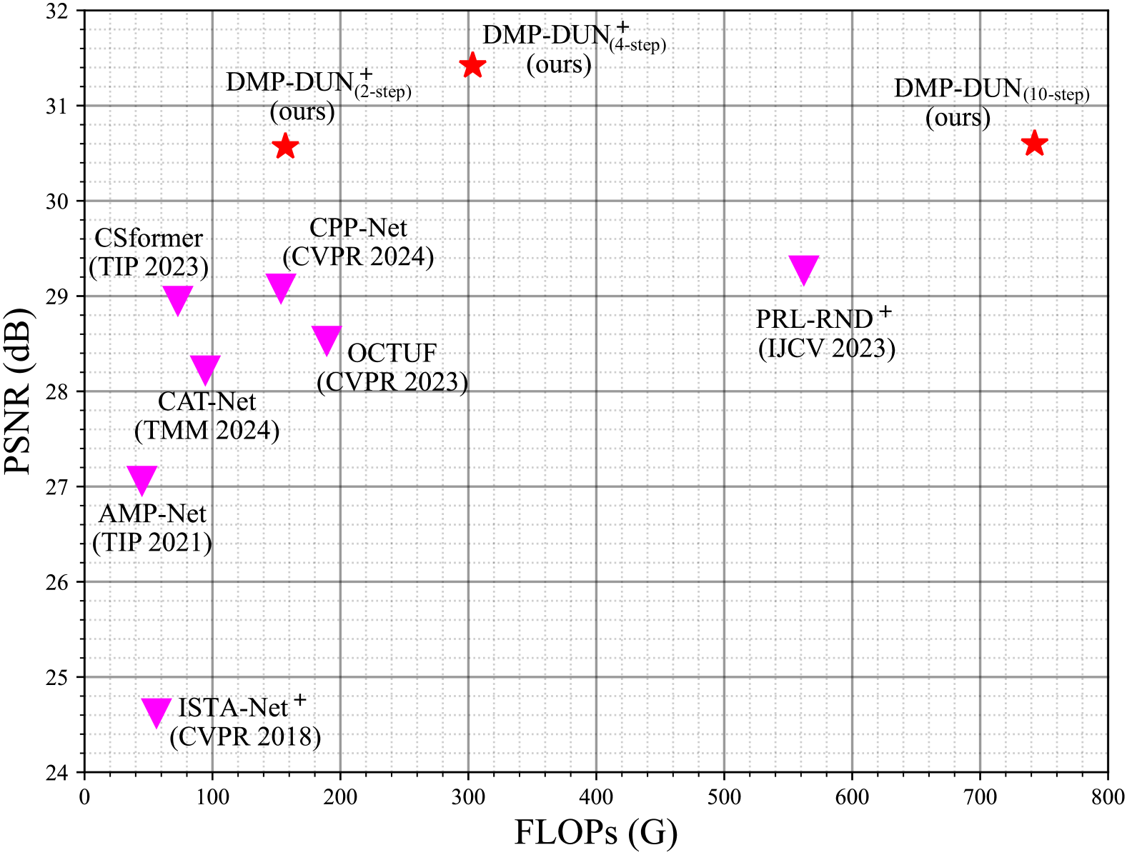
Figure 1: Comparison of the average PSNR and FLOPs of our proposed DMP-DUN with other methods on Urban100[18], under various CS ratio of 1%, 4%, 10%, 25% and 50%.

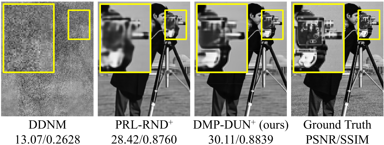
Figure 2: The reconstruction effects of different methods using only 2 steps under CS ratio = 10%.

1 Introduction

For the reason of utilizing the sparsity of the signal itself or its representation in some transform domain, Compressive Sensing (CS) can reconstruct signal from fewer measurements than conventional methods[6, 19]. Therefore, it has been widely applied in fields such as magnetic resonance imaging (MRI)[30, 34], snapshot compressive imaging (SCI)[11], and wireless tele-monitoring[60]. Mathematically, the sampling process of CS can be expressed as obtaining CS measurements $\operatorname{\mathbf{y}}=\operatorname{\mathbf{\Phi x}}+\epsilon$ from an original signal $\operatorname{\mathbf{x}}\in\mathbb{R}^{N}$ through the linear sensing matrix $\operatorname{\mathbf{\Phi}}\in\mathbb{R}^{M\times N}$ with Gaussian noise $\epsilon\in\mathbb{R}^{M}$, where $M\ll N$. CS is to infer the orginal signal $\operatorname{\mathbf{x}}$ by solving this ill-posed inverse problem with sensing rate $\delta=M/N$.

To overcome this problem, some transitional iterative optimization algorithms[16, 4, 20, 5, 1, 38] obtain approximate solutions by establishing an optimization model and iteratively optimizing. With the development of deep learning, some methods[31, 43, 53, 44, 55, 21] directly use neural networks to fit the mapping from CS measurements to ground truth, thus achieving higher reconstruction speed and quality.

More recently, Deep Unfolding Networks (DUNs) have become novel deep learning methods that are gaining attention in the field of image CS. DUNs[23, 54, 58, 61, 56, 42, 45, 48, 8, 24, 51, 15, 29] utilize the strengths of both traditional iterative algorithms and neural networks by unfolding each iteration of an optimization algorithm into a layer of a neural network, hence significantly improving convergence speed and reducing the number of iterations. At the same time, the prior knowledge learned during training is often richer than that manually designed in traditional iterative optimization algorithms, resulting in higher reconstruction quality.

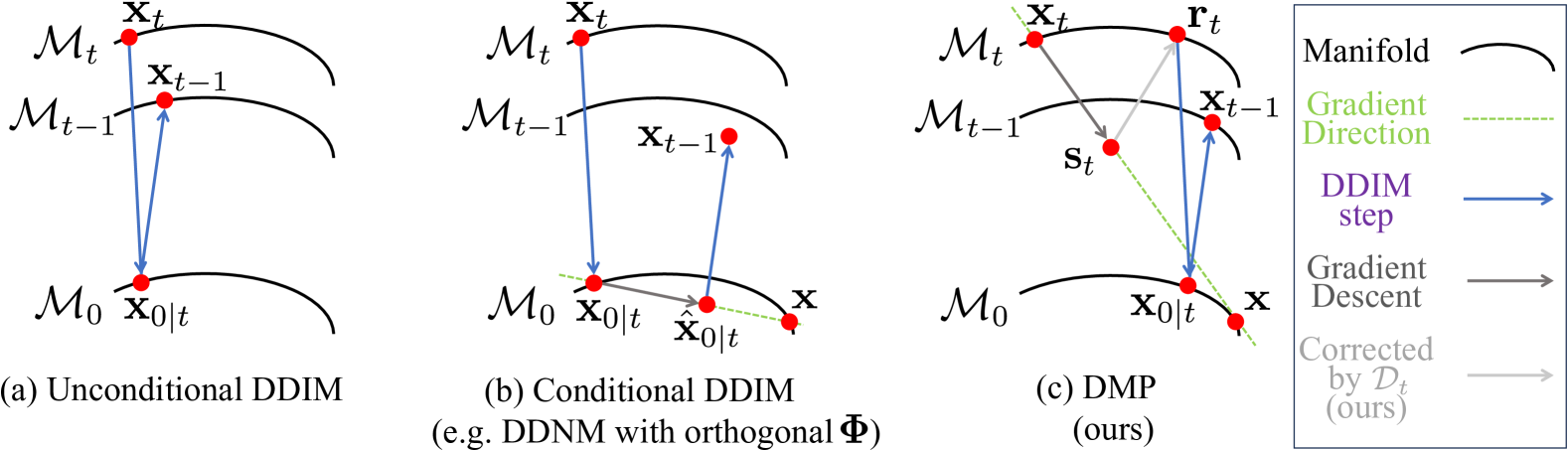
Figure 3: Compared with different type of diffusion models under the perspective of manifold hypothesis.

Meanwhile, pre-trained diffusion models[26, 46] possess powerful image prior knowledge, enabling high-quality image generation and reconstruction tasks. Currently, many methods[27, 52, 13, 25, 49, 14, 22, 40, 41] attempt to leverage diffusion models to solve linear inverse problems such as image CS. However, they predominantly require a large number of iterative steps, and perform unsatisfactorily at low CS ratios.

This prompts us to reflect that, on one hand, pre-trained diffusion models possess powerful image prior knowledge but require numerous iterative optimization steps to reconstruct images and have poor performance at low CS ratios. On the other hand, DUNs are a promising approach to mitigating the challenges posed by iterative optimization algorithms, which often necessitate numerous iterations and yield poor performance at low CS ratios. Consequently, can we propose a method that integrates pre-trained diffusion models with DUNs, thereby leveraging the powerful image prior knowledge to accomplish high-quality image CS reconstruction across various CS ratios with a reduced number of iterative steps?

In this paper, we attempt to embed pre-trained diffusion model into DUNs to achieve fast and high-quality image CS reconstruction under various CS ratios.

Firstly, we propose a new iterative optimization algorithm named Diffusion Message Passing (DMP), as shown in Eq. 5. This algorithm inspired by the classic CS algorithm Approximate Message Passing (AMP), and can embed one step of the reverse diffusion process into each iteration of DMP. By implementing each single step of reverse diffusion process through a pre-trained diffusion process, the objective of leveraging the powerful prior knowledge of the pre-trained diffusion model in DMP can be realized. Meanwhile, due to the design based on probabilistic graphical ideas and the utilization of statistical properties of data, DMP can provide faster convergence speeds compared to other methods[49, 14, 22, 40, 41] that use pre-trained diffusion models for reconstruction. Moreover, according to the state evolution of DMP (as shown in Eq. 6), the manifold-constrained states[25] of its variables during reconstruction can be represented as Fig. 3(c), which shows that our proposed DMP benefits from its unique state evolution to preserve the manifolds throughout reconstruction process, thereby enhancing the reconstruction quality.

Subsequently, we deeply unfold the proposed DMP into a neural network named DMP-DUN, as shown in Fig. 4. DMP-DUN can directly map CS measurements to the intermediate steps of the reverse diffusion process, and replace the Monte-Carlo SURE method[39] with a lightweight trainable network. Furthermore, we obtain the time steps and scaling parameters of DMP-DUN through end-to-end training, hence further improving the reconstruction process. Extensive experiments demonstrate that the reconstruction quality of our proposed method outperforms existing state-of-the-art methods with balanced computing cost (as shown in Fig. 1), and can use only 2 steps of DMP to achieve great reconstruction quality (as shown in Fig. 2).

In short, the main contributions of this paper can be summarized as follows:

• We propose an iterative optimization algorithm named DMP, which can embed pre-trained diffusion models in the step of iterations.

• We provide the state evolution equation of DMP, which demonstrates its capacity to maintain data manifolds throughout the reconstruction process and explains the enhancement in reconstruction quality.

• We propose DMP-DUN by deep unfolding DMP, which can replace a large number of steps in the reverse diffusion process and Monte-Carlo SURE method steps with a lightweight network, thereby saving a significant amount of time. Moreover, DMP-DUN can obtain time steps and scaling parameters through end-to-end training, which are hyper-parameters in the original diffusion model, thus further improving the reconstruction process.

• Extensive experiments show that our proposed DMP-DUN can outperform current state-of-the-art methods in terms of reconstruction quality with lower computational costs, requiring only at least 2 steps of DMP.

2 Related Work

2.1 Deep Unfolding Network

By treating CS problem as a Lasso problem, many iterative algorithms such as ISTA[16], FISTA[4], AMP[20], and etc. [5, 1], have been developed in the past few decades. In recent years, with the development of deep learning, several network-based methods[31, 43, 53, 44, 55, 21] have been proposed. Among them, a specific category known as Deep Unfolding Networks (DUNs)[23, 36, 54, 58, 61, 56, 42, 45, 48, 8, 24, 51, 15, 29] unfold the traditional iterative algorithms and implement some of their functions through neural networks, thereby achieving higher reconstruction quality than other network-based methods.

Early DUNs[23, 54, 58, 61] learned prior knowledge, such as sparse domains, through end-to-end training, significantly enhancing convergence speed and reconstruction quality. With the development of DUNs, methods like [45, 48] addressed information loss during iterations. Additionally, several approaches[56, 42, 8, 24, 51, 15, 29] further improved reconstruction quality and robustness by refining network structures. For example, Shen et al. [42] integrated Transformers, and Chen et al. [8] designed a multi-scale gradient descent network.

The effectiveness of these methods in reconstruction largely depends on the quality of the prior knowledge they learn. Although some methods[57, 63, 62] have been proposed to use pre-trained neural network as prior, there are no methods that utilize the powerful prior knowledge in pre-trained diffusion models.

2.2 Diffusion Model

In recent years, the diffusion model[26, 46] has attracted attention from many researchers due to its excellent image generation quality and the modifiability of the reverse diffusion process. Several works[27, 52, 13, 25, 49, 14, 22, 40, 41] attempted to leverage pre-trained diffusion models to solve inverse problems, such as image CS, image denoising and super-resolution. These works, such as DDNM[52] and MPGD[25], explored various strategies to adapt the diffusion process to the specific requirements of inverse problems, including modifying the diffusion steps, incorporating prior information, and optimizing the sampling techniques.

Meanwhile, some methods[9, 12, 7, 37] achieve higher quality reconstruction in natural image CS and MRI through redefining reverse diffusion process and retraining the diffusion model. Specifically, Chen et al. [9] proposed the Invertible Diffusion Model (IDM), which implements end-to-end training of diffusion models, significantly improving the reconstruction quality and efficiency of diffusion models in image CS.

Compared to these methods, our proposed DMP-DUN can achieve higher quality reconstruction with fewer steps by unfolding our proposed DMP algorithm which embeds a diffusion model.

3 Notation and Definitions

This paper uses mathematical boldface to represent tensors, with uppercase boldface for matrices. The normal distribution is denoted by $\mathcal{N}$, and the identity matrix by $\operatorname{\mathbf{I}}$. The sets of real numbers and natural numbers are denoted by $\operatorname{\mathbb{R}}$ and $\mathbb{N}$, respectively.

Traditional iterative optimization algorithms start at $t=0$ and converge to the theoretical optimal solution at $t=+\infty$. In contrast, the reconstruction process of diffusion models begins at $t=+\infty$ and results in the reconstructed image at $t=0$. Therefore, to ensure that the iterative processes of the two methods match, this paper standardizes $t=+\infty$ as the starting point of iteration and $t=0$ as the end point.

We employ the block-based compressive sensing method[50, 59], which divides the image into non-overlapping blocks of size $B\times B$ and flattens each block, where $B^{2}=N$. For simplicity, we implicitly assume that the image has been divided and flattened into a one-dimensional tensor when performing left-multiplication matrix throughout this paper.

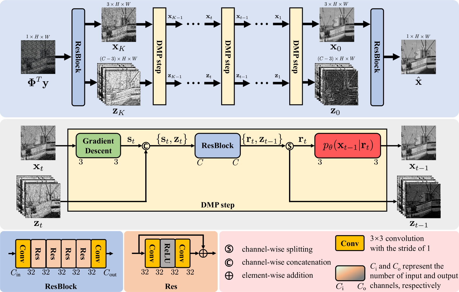
Figure 4: The reconstruction process of our proposed DMP-DUN, where DMP step represents each iteration of Diffusion Message Passing (DMP) with pre-trained Diffusion Model (i.e. $p_{\theta}(\operatorname{\mathbf{x}}_{t-1}|\operatorname{\mathbf{r}}_{t})$).

4 Method

4.1 Preliminaries

The original image $\mathbf{x}\in\mathbb{R}^{N}$ is obtained through the sensing matrix $\mathbf{\Phi}\in\mathbb{R}^{M\times N}$, resulting in CS measurements $\mathbf{y}\in\mathbb{R}^{M}$, where $M\ll N$. The problem of reconstructing $\mathbf{x}$ from the known $\mathbf{y}$ and $\mathbf{\Phi}$ can be formulated as the following optimization problem:

$$\hat{\operatorname{\mathbf{x}}}=\mathop{\arg\min}_{\operatorname{\mathbf{x}}}\|\operatorname{\mathbf{y}}-\operatorname{\mathbf{\Phi x}}\|_{2}^{2}\qquad\text{s.t. }\operatorname{\mathbf{x}}\in\mathcal{X}$$ (1)

where $\|\cdot\|_{2}$ means $\ell_{2}$ norm, $\mathcal{X}\subset\mathbb{R}^{N}$ represents a set constrained by certain prior knowledge. For example, $\mathcal{X}$ can be defined as the collection of all sparse representations in a specific transform domain (such as the DCT domain) for natural images. In addressing this problem, AMP makes the following assumptions:

Assumption 1.

The Gaussian sensing matrix $\mathbf{\Phi}\sim\mathcal{N}(0,\operatorname{\mathbf{I}}/M)$. The sensing rate $\delta=M/N\in\mathbb{R}(0,1)$, where $M,N\to+\infty$. The denoising function $\eta_{t}(\cdot)$ is Lipschitz continuous, with $t\in\mathbb{N}$.

Based on the above assumption, AMP gives the following iterative formula to reconstruct the image with the iteration starts from $t=+\infty$ and ends when $t=0$, and the final answer $\operatorname{\mathbf{x}}_{0}$ will be converged to ground truth:

$$\operatorname{\mathbf{u}}_{t} =\operatorname{\mathbf{y}}-\operatorname{\mathbf{\Phi x}}_{t}+\operatorname{\mathbf{u}}_{t+1}\text{div}\eta_{t}(\operatorname{\mathbf{h}}_{t+1})/M$$ (2)

$$\operatorname{\mathbf{h}}_{t} =\operatorname{\mathbf{\Phi}^{T}\mathbf{u}}_{t}+\operatorname{\mathbf{x}}_{t}$$

$$\operatorname{\mathbf{x}}_{t-1} =\eta_{t}(\operatorname{\mathbf{h}}_{t})$$

where $\text{div}(\cdot)$ represents the divergence and the term $[\operatorname{\mathbf{u}}_{t+1}\text{div}\eta_{t}(\operatorname{\mathbf{h}}_{t+1})/M]$ in AMP is referred to as the Onsager term. If the denoiser $\eta_{t}(\cdot)$ is a black-box function such as a deep neural network, then its divergence can be approximated through the method of Monte Carlo approximation[39, 35], that is, by using $\mathbf{g}[\eta_{t}(\operatorname{\mathbf{h}}_{t+1}+\varepsilon\mathbf{g})-\eta_{t}(\operatorname{\mathbf{h}}_{t+1})]/\varepsilon$ to approximate divergence of $\eta_{t}(\cdot)$, where $\mathbf{g}\sim\mathcal{N}(0,\operatorname{\mathbf{I}})$ and $\varepsilon\to 0$. Onsager term can decouple the errors across iterations, resulting in the iterative formula that approximately follows the following state evolution:

$$\operatorname{\mathbf{h}}_{t} \sim\mathcal{N}(\operatorname{\mathbf{x}},\sigma^{2}_{t}\operatorname{\mathbf{I}}/\delta)$$ (3)

$$\sigma^{2}_{t-1} =\mathbb{E}\left\{[\eta_{t}(\operatorname{\mathbf{h}}_{t})-\operatorname{\mathbf{x}}]^{2}\right\}$$

4.2 Diffusion Message Passing Algorithm

In this sub-section, we will elaborate how the Diffusion Message Passing (DMP) algorithm embeds a pre-trained diffusion model into its iterations to harness prior knowledge.

In the diffusion model[26, 46], for the original image $\operatorname{\mathbf{x}}$, let $\alpha_{t}\in\mathbb{R}[0,1]$ decrease with increasing $t\in\mathbb{N}$, where the scaling parameter $\alpha_{0}=1$. The forward diffusion process start at $\operatorname{\mathbf{x}}_{0}=\operatorname{\mathbf{x}}$, and at the $t$-th step is given by $q(\operatorname{\mathbf{x}}_{t}|\operatorname{\mathbf{x}}_{t-1})=\mathcal{N}(\sqrt{\alpha_{t}}\operatorname{\mathbf{x}}_{t-1},(1-\alpha_{t})\operatorname{\mathbf{I}})$. The parameter $\alpha_{t}=0$ when $t=+\infty$, so at this time $\operatorname{\mathbf{x}}_{t}\sim\mathcal{N}(\mathbf{0},\operatorname{\mathbf{I}})$. Under the assumption that $\operatorname{\mathbf{x}}_{0}$ is known, the denosing diffusion model can obtain the reverse diffusion process as follows:

$$q(\operatorname{\mathbf{x}}_{t-1}|\operatorname{\mathbf{x}}_{t},\operatorname{\mathbf{x}}_{0})=\mathcal{N}(\tilde{\mu_{t}}(\operatorname{\mathbf{x}}_{t},\operatorname{\mathbf{x}}_{0}),\tilde{\beta_{t}}\operatorname{\mathbf{I}})$$ (4)

where $\tilde{\mu}(\operatorname{\mathbf{x}}_{t},\operatorname{\mathbf{x}}_{0})=\frac{1-\bar{\alpha}_{t-1}}{1-\bar{\alpha}_{t}}\sqrt{\alpha_{t}}\operatorname{\mathbf{x}}_{t}+\frac{1-\alpha_{t}}{1-\bar{\alpha}_{t}}\sqrt{\bar{\alpha}_{t-1}}\operatorname{\mathbf{x}}_{0}$, $\tilde{\beta_{t}}=\frac{1-\bar{\alpha}_{t-1}}{1-\bar{\alpha}_{t}}(1-\alpha_{t})$, and $\bar{\alpha}_{t}=\prod_{i=1}^{t}\alpha_{i}$. For $\operatorname{\mathbf{x}}_{0}$ is unknown in practical scenarios, diffusion model use $p_{\theta}(\operatorname{\mathbf{x}}_{t-1}|\operatorname{\mathbf{x}}_{t})$ to approximate $q(\operatorname{\mathbf{x}}_{t-1}|\operatorname{\mathbf{x}}_{t},\operatorname{\mathbf{x}}_{0})$, where $\theta$ represents the learnable parameters in the network.

Assumption 2.

The neural network $p_{\theta}(\operatorname{\mathbf{x}}_{t-1}|\operatorname{\mathbf{x}}_{t})$ is a perfect denoiser, meaning $p_{\theta}(\operatorname{\mathbf{x}}_{t-1}|\operatorname{\mathbf{x}}_{t})\equiv q(\operatorname{\mathbf{x}}_{t-1}|\operatorname{\mathbf{x}}_{t},\operatorname{\mathbf{x}}_{0})$. Consequently, $\operatorname{\mathbf{x}}_{t}\sim\mathcal{N}(\sqrt{\bar{\alpha}_{t}}\operatorname{\mathbf{x}},(1-\bar{\alpha}_{t})\operatorname{\mathbf{I}})$ for all $t\in\mathbb{N}$.

Assumption 3.

A perfect Gaussian filter exists and is represented by $\mathcal{D}_{t}(\cdot)$. The distribution $q(\mathcal{D}_{t}(\operatorname{\mathbf{d}}_{t})|\operatorname{\mathbf{d}}_{t})=\mathcal{N}(\sqrt{\bar{\alpha}_{t}}\operatorname{\mathbf{x}},(1-\sqrt{\bar{\alpha}_{t}})\operatorname{\mathbf{I}})$, where $\operatorname{\mathbf{d}}_{t}\sim\mathcal{N}(\sqrt{\bar{\alpha}_{t}}\operatorname{\mathbf{x}},(1-\sqrt{\bar{\alpha}_{t}})\operatorname{\mathbf{I}}/\delta)$.

Based on the aforementioned description and considering the diffusion model as a denoiser, we can derive the following theorem for our proposed DMP algorithm:

Theorem 1.

Suppose Assumption 1, 2, and 3 hold, we deduce the iterative representation of Diffusion Message Passing (DMP) algorithm as follows:

$$\operatorname{\mathbf{s}}_{t} =\operatorname{\mathbf{x}}_{t}-\sqrt{\operatorname{\bar{\alpha}}_{t}}\operatorname{\mathbf{\Phi}}^{\mathrm{T}}(\operatorname{\mathbf{\Phi x}}_{t}-\operatorname{\mathbf{y}})$$ (5)

$$\operatorname{\mathbf{r}}_{t} =\mathcal{D}_{t}[\operatorname{\mathbf{s}}_{t}+\sqrt{\operatorname{\bar{\alpha}}_{t}}o_{t}(\operatorname{\mathbf{u}}_{t+1},\operatorname{\mathbf{h}}_{t+1})]$$

$$\operatorname{\mathbf{x}}_{t-1} =p_{\theta}(\operatorname{\mathbf{x}}_{t-1}|\operatorname{\mathbf{r}}_{t})$$

where $o_{t}(\operatorname{\mathbf{u}}_{t+1},\operatorname{\mathbf{h}}_{t+1}):=\operatorname{\mathbf{\Phi}}^{\mathrm{T}}\operatorname{\mathbf{u}}_{t+1}\mathrm{div}\eta_{t}(\operatorname{\mathbf{h}}_{t+1})$. Moreover, it is possible to write out its state evolution:

$$\operatorname{\mathbf{r}}_{t} \sim\mathcal{N}(\sqrt{\operatorname{\bar{\alpha}}_{t}}\operatorname{\mathbf{x}},\sigma^{2}_{t}\operatorname{\mathbf{I}})$$ (6)

$$\sigma^{2}_{t-1} =\mathbb{E}\left\{[p_{\theta}(\operatorname{\mathbf{x}}_{t-1}|\operatorname{\mathbf{r}}_{t})-\sqrt{\operatorname{\bar{\alpha}}_{t-1}}\operatorname{\mathbf{x}}]^{2}\right\}$$

Due to space constraints, we relegate the detailed proof to Supplementary Materials for Theorem 1.

4.3 DMP-DUN

Although Theorem 1 can be derived under the Assumptions 1, 2, and 3, it is hard to fully meet these assumptions in practical problems. Furthermore, the term $o_{t}(\operatorname{\mathbf{u}}_{t+1},\operatorname{\mathbf{h}}_{t+1})$ in Eq. 5 necessitates the computation of divergence of the denoiser. When the denoiser is a black box, it becomes imperative to employ the Monte-Carlo SURE[39] method for resolution, which thus doubles the computational expense relative to the denoiser itself. Considering the success of DUN in the CS field, we propose a novel method named DMP-DUN in this paper, which deeply unfolds DMP algorithm and introduces several convolutional residual blocks (ResBlocks) to implement functions such as $o_{t}$ and $\mathcal{D}_{t}$ within Eq. 5. Moreover, DMP-DUN enables the learning of what were traditionally hyper-parameters like $\operatorname{\bar{\alpha}}_{t}$ and $t$, which previously required manual tuning in diffusion models.

The specific structure of DMP-DUN is illustrated in Fig. 4, where each DMP step denotes an iterative step of DMP algorithm (i.e. Eq. 5). Specifically, the Gradient Descent, ResBlock, and $p_{\theta}(\operatorname{\mathbf{x}}_{t-1}|\operatorname{\mathbf{r}}_{t})$ in DMP represent the steps for obtaining $\operatorname{\mathbf{s}}_{t}$, $\operatorname{\mathbf{r}}$, and $\operatorname{\mathbf{x}}_{t-1}$ in Eq. 5, respectively. Additionally, We place the ResBlock at the head and the tail of DMP-DUN, respectively. The ResBlock at head of DMP-DUN can save the time required for the reverse diffusion process from $T$ to $K$ by processing the input image $\operatorname{\mathbf{\Phi}^{T}\mathbf{y}}$ into an image $\operatorname{\mathbf{x}}_{K}$ that conforms to the distribution of the diffusion model at time $K$, where the $K$ is less than the start time $T$ of the original diffusion model. The feature map $\operatorname{\mathbf{z}}_{t}$ can be represented as $\operatorname{\mathbf{z}}_{t}(\operatorname{\mathbf{u}}_{t+1},\operatorname{\mathbf{h}}_{t+1})$ according to the definitions in Eq. 2 and (5) and can be applied in the subsequent DMP step, where the initial feature map $\operatorname{\mathbf{z}}_{K}$ is also generated by the ResBlock at head of DMP-DUN. The ResBlock at the end of DMP-DUN functions to transform the final RGB image output of the DMP into a single-channel image, thereby constructing the bridge between the RGB image processed by a pre-trained diffusion model and the Y-channel image that needs to be reconstructed.

Method Set11[31] Avg. FLOPs 1% 4% 10% 25% 50% (G) ISTA-Net⁺[58] (CVPR 2018) 17.45/0.4131 21.56/0.6240 26.49/0.8036 32.44/0.9237 38.08/0.9680 27.20/0.7465 56.2 AMP-Net[61] (TIP 2021) 20.20/0.5581 25.26/0.7722 29.40/0.8779 34.63/0.9481 40.34/0.9807 29.97/0.8274 44.9 TransCS[42] (TIP 2022) 20.15/0.5066 25.41/0.7883 29.54/0.8877 35.06/0.9548 40.21/0.9824 29.02/0.8174 26.6 CSformer[55] (TIP 2023) 21.58/0.6075 26.28/0.8062 29.79/0.8883 34.81/0.9527 40.73/0.9824 31.21/0.8584 72.9 DPC-DUN[47] (TIP 2023) 18.03/0.4601 24.38/0.7498 29.42/0.8801 34.75/0.9483 39.84/0.9778 29.28/0.8032 138.0 OCTUF[48] (CVPR 2023) 21.75/0.5934 26.45/0.8126 30.70/0.9030 36.10/0.9604 41.34/0.9838 31.27/0.8506 189.3 PRL-RND⁺[8] (IJCV 2023) 22.27/0.6240 26.88/0.8130 31.66/0.9189 36.69/0.9608 41.84/0.9850 31.87/0.8603 562.2 CAT-Net[29] (TMM 2024) 21.29/0.5782 26.38/0.8060 30.69/0.9022 35.85/0.9588 41.28/0.9834 31.10/0.8457 94.4 UFC-Net[51] (CVPR 2024) 21.24/0.5607 25.92/0.7943 30.15/0.8960 35.42/0.9567 - - 109.0 CPP-Net[24] (CVPR 2024) 22.19/0.6135 27.23/0.8337 31.27/0.9135 36.35/0.9631 41.39/0.9827 31.69/0.8613 153.5 DDNM${}_{\text{(10-step)}}$[52] (ICLR 2023) 11.89/0.1748 12.29/0.1338 13.39/0.1404 16.98/0.2959 25.63/0.8074 16.04/0.3105 670.4 DDNM${}^{+}_{\text{(1000-step)}}$[52] (ICLR 2023) 17.95/0.4497 22.54/0.6827 25.78/0.8154 27.80/0.8933 29.01/0.9411 24.62/0.7564 67039.1 DMP-DUN${}_{\text{(10-step)}}$ (ours) 23.32/0.6305 28.20/0.8340 32.51/0.9161 37.92/0.9668 42.99/0.9857 32.99/0.8666 742.6 DMP-DUN${}^{+}_{\text{(2-step)}}$ (ours) 23.18/0.6286 28.25/0.8360 32.63/0.9206 37.58/0.9648 42.06/0.9835 32.74/0.8667 157.0 DMP-DUN${}^{+}_{\text{(4-step)}}$ (ours) 23.32/0.6313 28.67/0.8448 33.22/0.9277 38.29/0.9681 42.82/0.9848 33.26/0.8713 303.4

Method Urban100[18] Avg. FLOPs 1% 4% 10% 25% 50% (G) ISTA-Net⁺[58] (CVPR 2018) 16.66/0.3733 19.65/0.5368 23.48/0.7200 28.89/0.8830 34.43/0.9571 24.62/0.6940 56.2 AMP-Net[61] (TIP 2021) 19.55/0.5016 22.73/0.6819 25.92/0.8144 30.79/0.9188 36.33/0.9712 27.06/0.7776 44.9 TransCS[42] (TIP 2022) 18.96/0.4395 23.25/0.7114 26.74/0.8416 31.75/0.9329 37.20/0.9761 27.58/0.7803 26.6 CSformer[55] (TIP 2023) 21.57/0.5672 24.94/0.7396 27.92/0.8458 32.43/0.9332 37.88/0.9766 28.95/0.8125 72.9 DPC-DUN[47] (TIP 2023) 17.28/0.4214 22.35/0.6767 26.94/0.8358 32.33/0.9320 37.52/0.9737 27.28/0.7679 138.0 OCTUF[48] (CVPR 2023) 19.88/0.5167 23.68/0.7329 27.79/0.8621 32.99/0.9445 38.29/0.9797 28.53/0.8072 189.3 PRL-RND⁺[8] (IJCV 2023) 20.63/0.5632 24.32/0.7439 28.75/0.8743 34.00/0.9483 38.64/0.9798 29.27/0.8219 562.2 CAT-Net[29] (TMM 2024) 19.63/0.5209 23.64/0.7188 27.59/0.8485 32.48/0.9340 37.77/0.9751 28.22/0.7995 94.4 UFC-Net[51] (CVPR 2024) 19.69/0.5041 23.37/0.7195 27.55/0.8583 32.82/0.9423 - - 109.0 CPP-Net[24] (CVPR 2024) 20.55/0.5554 24.66/0.7691 28.49/0.8801 33.38/0.9485 38.33/0.9781 29.08/0.8262 153.5 DDNM${}_{\text{(10-step)}}$[52] (ICLR 2023) 10.53/0.1374 11.00/0.1210 12.26/0.1441 16.28/0.3293 24.81/0.8147 14.98/0.3093 670.4 DDNM${}^{+}_{\text{(1000-step)}}$[52] (ICLR 2023) 17.48/0.4114 21.86/0.6435 24.62/0.7880 26.22/0.8621 27.35/0.9118 23.51/0.7234 67039.1 DMP-DUN${}_{\text{(10-step)}}$ (ours) 21.48/0.5671 25.80/0.7727 30.04/0.8857 35.25/0.9538 40.44/0.9827 30.60/0.8324 742.6 DMP-DUN${}^{+}_{\text{(2-step)}}$ (ours) 21.66/0.5750 26.25/0.7858 30.41/0.8922 35.07/0.9520 39.46/0.9795 30.57/0.8369 157.0 DMP-DUN${}^{+}_{\text{(4-step)}}$ (ours) 21.80/0.5832 26.98/0.8035 31.39/0.9053 36.14/0.9584 40.80/0.9827 31.42/0.8466 303.4

Table 1: Average PSNR/SSIM performance comparisons of various CS methods on Set11[31] and Urban100[18]. The best and second best results are highlighted in red and blue colors, respectively. The best results among the compared methods are highlighted with underlines.

In the Gradient Descent module, we use a learnable parameter $\lambda_{t}\in\mathbb{R}^{+}$ to replace $\sqrt{\bar{\alpha}}_{t}$ in Eq. 5 to increase fault tolerance, and the formula is as follows:

$$\operatorname{\mathbf{s}}_{t}=\operatorname{\mathbf{x}}_{t}-\lambda_{t}\operatorname{\mathbf{\Phi}}^{\mathrm{T}}(\operatorname{\mathbf{\Phi x}}_{t}-\operatorname{\mathbf{y}})$$ (7)

To obtain the $\operatorname{\mathbf{r}}_{t}$ in Eq. 5, we proposed to directly use a lightweight neural network to fit the $\mathcal{D}_{t}$ and learn how to get the onsager term directly by using the ResBlock:

$$\{\operatorname{\mathbf{r}}_{t},\operatorname{\mathbf{z}}_{t-1}\}=\mathcal{H}_{\text{Conv}}\left(\mathcal{H}_{\text{4-Res}}\left(\mathcal{H}_{\text{Conv}}\left(\{\operatorname{\mathbf{s}}_{t},\operatorname{\mathbf{z}}_{t}\}\right)\right)\right)$$ (8)

where $\mathcal{H}_{\text{Conv}}$ is a $3\times 3$ convolution with stride is 1, and $\mathcal{H}_{\text{4-Res}}$ denotes 4 cascaded Res structures. Each Res structure use $\operatorname{\mathbf{x}}+\mathcal{H}_{\text{Conv}}(\text{ReLU}(\mathcal{H}_{\text{Conv}}(\operatorname{\mathbf{x}})))$ to implement. The resultant output $\mathbf{z}_{t-1}$ is utilized in the subsequent iteration of the DMP step.

Subsequently, $\mathbf{r}_{t}$ serves as the input for the ensuing module $p_{\theta}(\mathbf{x}_{t-1}|\mathbf{r}_{t})$, which is implemented using a pre-trained diffusion model. Such integration can leverage powerful prior knowledge of the pre-trained diffusion model, and can compatible with various diffusion models.

4.4 DMP-DUN⁺

Instead of freezing the parameters of diffusion model when training DMP-DUN, the proposed DMP-DUN⁺ allows them to be unfrozen during training. This approach will significantly increase the training cost but can further improve the reconstruction quality. Additionally, this operation only affects the training cost and does not impact the cost of using it for reconstruction.

4.5 End-to-End Learning

Unlike diffusion models which trained to minimize the local reverse diffusion process between $q(\operatorname{\mathbf{x}}_{t-1}|\operatorname{\mathbf{x}}_{t},\operatorname{\mathbf{x}}_{0})$ and $p_{\theta}(\operatorname{\mathbf{x}}_{t-1}|\operatorname{\mathbf{x}}_{t})$ as the optimization target, our proposed DMP-DUN and DMP-DUN⁺ uses the training strategy of DUNs that employs end-to-end training to directly optimize the entire reconstruction process. Given a set of full-sampled images $\{\mathbf{x}_{i}\}_{i=1}^{N_{a}}$ and its CS measurements set $\{\operatorname{\mathbf{y}}_{i}|\operatorname{\mathbf{y}}_{i}=\operatorname{\mathbf{\Phi x}}_{i}\}_{i=1}^{N_{a}}$, we use the mean squared error (MSE) as the loss function. We update all parameters in DMP-DUN except for the parameters in pre-trained diffusion model. For DMP-DUN⁺, we update all parameters including those of diffusion model. The training objective of DMP-DUN and DMP-DUN⁺ can be represented as shown below:

$$\min\limits_{\mathbf{\Theta}}\frac{1}{N_{p}N_{a}}\sum^{N_{a}}_{i=1}\|\mathcal{F}_{\mathbf{\Theta}}(\operatorname{\mathbf{\Phi}^{T}\mathbf{y}}_{i})-\operatorname{\mathbf{x}}_{i}\|_{2}^{2}$$ (9)

where $\mathcal{F}_{\mathbf{\Theta}}$ denotes the entire reconstruction process of DMP-DUN or DMP-DUN⁺, $N_{a}$ is the size of training dataset, $N_{p}$ is the number of pixels in each image $\mathbf{x}_{i}$. $\mathbf{\Theta}$ denotes the set of all trainable parameters of DMP-DUN or DMP-DUN⁺, which includes the trainable sensing matrix $\operatorname{\mathbf{\Phi}}$.

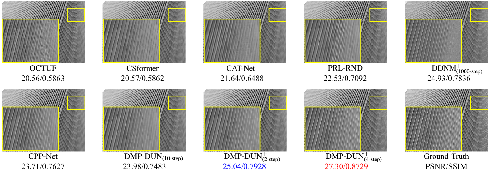
Figure 5: The comparison of the subjective visual effects between our proposed DMP-DUN, DMP-DUN⁺, and other methods at CS ratio = 4%. The best and second best results are highlighted in red and blue colors, respectively.

Urban100[18] DIV2K[2] Method 10% 30% 50% 10% 30% 50% Avg. DDNM⁺ (ICLR’23) 24.61 26.74 27.71 24.40 26.61 27.73 26.30 IDM     (TPAMI’25) 31.41 36.76 40.33 31.07 36.98 41.15 36.28 DMP-DUN⁺  (ours) 31.90 37.45 41.58 32.56 38.32 42.66 37.41

Table 2: Average PSNR performance comparisons of various methods based on diffusion model with $256\times 256$ center-cropped.

Method Pre-trained Set11 Urban100 Avg. 4% 25% 4% 25% CSformer[55] ✗ 26.28/0.8062 34.81/0.9527 24.94/0.7396 32.43/0.9332 29.62/0.8579 PRL-RND⁺[8] ✗ 26.88/0.8130 36.69/0.9608 24.32/0.7439 34.00/0.9483 30.47/0.8665 CPP-Net[24] ✗ 27.23/0.8337 36.35/0.9631 24.66/0.7691 33.38/0.9485 30.41/0.8786 DMP-DUN${}^{+}_{\text{(4-step)}}$ ✓ 28.67/0.8448 38.29/0.9681 26.98/0.8035 36.14/0.9584 32.52/0.8937 DMP-DUN${}^{+}_{\text{(4-step)}}$ ✗ 28.43/0.8407 38.07/0.9672 26.28/0.7878 35.63/0.9557 32.10/0.8879

Table 3: Comparison of DMP-DUN⁺ with and without loading the pre-trained parameter at the begin of training.

Case Gradient Descent ResBlock $p_{\theta}(\mathbf{x}_{t-1}|\mathbf{r}_{t})$ Set11 Set14 Urban100 Avg. (a) ✗ ✓ ✓ 29.89/0.8713 28.77/0.8015 27.27/0.8225 28.64/0.8318 (b) ✓ ✗ ✓ 32.14/0.9097 31.04/0.8476 29.73/0.8702 30.97/0.8758 (c) ✓ ✓ ✗ 31.89/0.9009 30.82/0.8423 29.14/0.8627 30.62/0.8686 DMP-DUN${}^{+}_{\text{(4-step)}}$ ✓ ✓ ✓ 33.22/0.9277 31.71/0.8664 31.39/0.9053 32.11/0.8998

Table 4: Ablation study of DMP-DUN at CS ratio = 10%.

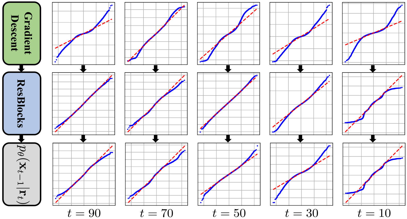
Figure 6: Q-Q plots for the noise in output images of each module in DMP step at different $t$. The horizontal axis represents the quantiles of normal distribution and the vertical axis represents the quantiles of noise. The closer the distribution of the blue points is to the red line, the more the noise conforms to a normal distribution.

Steps 2 4 5 10 Set11 31.39/0.9030 32.02/0.9091 32.12/0.9106 32.51/0.9161 Urban100 28.47/0.8600 29.28/0.8728 29.57/0.8776 30.04/0.8857

Table 5: Average PSNR/SSIM performance comparisons of various iterative steps of DMP-DUN under CS ratio = 10%.

5 Experiment

5.1 Experimental Settings

We set the block size $B=64$, and the number of measurements $M=\lfloor\delta N\rfloor$, where $\delta\in\{1\%,4\%,10\%,25\%,50\%\}$ is the CS ratio. The channel numbers $C$ is set as $32$. The DMP-DUN and DMP-DUN⁺ employ the technique from DDIM[46] to accelerate the reverse diffusion process with initial time $K=100$. We use the pre-trained diffusion model on $256\times 256$ image in ImageNet dataset by [17]. According to different acceleration step size $\Delta t$, we propose three methods: DMP-DUN${}_{\text{(10-step)}}$ with $\Delta t=10$, DMP-DUN${}^{+}_{\text{(4-step)}}$ with $\Delta t=25$, and DMP-DUN${}^{+}_{\text{(2-step)}}$ with $\Delta t=50$. The FLOPs is calculated using an input image of size $256\times 256$.

We trained on 118K images from COCO2017[32] and validated on 100 images from BSDS500[3]. Images are converted to YCbCr space, using Y-channel for training, validation and testing. Each training epoch crops 118K random $64\times 64$ patches from COCO2017 with randomly horizontal flipping. We used Adam[28] as the optimizer with $(\beta_{1},\beta_{2})=(0.9,0.999)$ and the default batch size is 8. The model is trained for 20 epochs with an initial learning rate of $1\times 10^{-4}$, which is decreased to $1\times 10^{-6}$ using the cosine annealing strategy[10, 33]. The model is implemented using PyTorch and trained on a single NVIDIA RTX3090 GPU.

5.2 Reconstruction Quality Evaluation

The reconstruction quality evaluation in this sub-section is divided into objective metrics comparison (Tab. 1 and Tab. 2) and subjective visual effects comparison (Fig. 5).

We utilize PSNR/SSIM as objective metrics to compare with several SOTA methods on Set11 [31] and Urban100 [18], as shown in Tab. 1. It can be seen that our proposed DMP-DUN${}^{+}_{\text{(4-step)}}$ achieves average PSNR values higher than PRL-RND⁺[8] by 1.39dB and 2.15dB on Set11 and Urban100, respectively, with fewer FLOPs by 258.8G. Additionally, our proposed DMP-DUN${}^{+}_{\text{(2-step)}}$ improves the PSNR by 1.05dB and 1.49dB on Set11 and Urban100, respectively, while maintaining similar FLOPs to CPP-Net[24].

Additionally, we compare our method with the Invertible Diffusion Model (IDM)[9], which also employs end-to-end training of pre-trained diffusion models. Since IDM used $256\times 256$ crop size, we retrained DMP-DUN${}^{+}_{\text{(4-step)}}$ under identical settings, as shown in Tab. 2. Our method achieves 1.23dB higher average PSNR than IDM. As IDM has demonstrated at least 5.55dB PSNR superiority over other diffusion-based methods[49, 14, 22, 40, 41], our approach logically surpasses these methods in reconstruction quality.

The subjective visual effects in Fig. 5 show that our method is able to more realistically reflect the textures on the buildings without any blurring or confusing phenomena.

Moreover, since most of the methods compared in Tab. 1 did not use pre-trained models, to ensure the fairness of experiment, we compared the DMP-DUN⁺ without using pre-trained weights with several methods[55, 8, 24], as shown in Tab. 3. It can be seen that average PSNR of DMP-DUN${}^{+}_{\text{(4-step)}}$ without using pre-trained weights decreased by 0.42dB, but it still performed better than other state-of-the-art methods. This not only demonstrates that the powerful prior knowledge contained in pre-trained models can effectively improve reconstruction quality, but also shows that our algorithm is reasonable and robust, allowing it to perform well even without using pre-trained prior knowledge.

5.3 Effect of Resblock for Decoupling Errors

In our proposed DMP-DUN, we utilize ResBlock to achieve the acquisition of the AMP Onsager term, thereby ensuring that the difference between the output image and the true image (i.e. the contained noise) follows a Gaussian distribution. Fig. 6 shows the Q-Q plots for the noise in output images of each module in DMP step of DMP-DUN${}_{\text{(10-step)}}$ at different $t$ during the Monarch image reconstruction process on the Set11 dataset. It can be observed from the figure that the noise in the images output by the ResBlock module basically follows a Gaussian distribution, confirming that it indeed can decouple the error from the image output by the preceding Gradient Descent module.

5.4 Ablation Study

We conducted an ablation study on the three modules of DMP step in DMP-DUN⁺, as shown in Tab. 4. Cases (a), (b), and (c) demonstrate that all three modules in DMP significantly impact the reconstruction quality. Moreover, Tab. 5 shows the effect of different iterative steps on the reconstruction quality in DMP-DUN.

5.5 Complexity study

Metrics DDNM${}^{+}_{\text{(1000-step)}}$[52] DMP-DUN${}^{+}_{\text{(4-step)}}$ (ours) 1 step 1000 steps 1 step Side-ResBlcoks 4 steps FLOPs (G) 67.0 67039.1 73.2 10.6 303.4 Params. (M) 552.8 552.8 552.9 0.2 553.4 PSNR (dB) 32.34 24.07

Table 6: Comparison of DDNM and DMP-DUN⁺ on average PSNR of Set11 and Urban100

Metrics Monte-Carlo SURE[39] ResBlock (ours) 1 step 4 steps 1 step 4 steps FLOPs (G) 134.1 536.4 6.1 24.4 Params. (M) 0 0 0.09 0.37

Table 7: Comparison of using ResBlock to replace Monte-Carlo SURE for computing the Onsager term in DMP-DUN.

The complexity of DMP-DUN⁺ compared to DDNM⁺[52], which is also based on the diffusion model approach, is illustrated in Tab. 6. Our method increases FLOPs by 6.2G per step but reduces the number of steps from 1000 to 4, while improving the reconstruction quality.

The complexity of using ResBlock as a replacement for Monte-Carlo SURE[39] is shown in Tab. 7. It can be seen that the use of ResBlock for approximation can save a total of approximately 512.0G FLOPs.

6 Conclusion

In this work, we design an iterative optimization algorithm named DMP, which leverages the powerful prior knowledge of pre-trained diffusion models while maintaining the manifold-constrained states according to its state evolution. We then unfold DMP into networks named DMP-DUN and DMP-DUN⁺, which utilize lightweight neural networks to approximate Gaussian filters and Monte-Carlo SURE through end-to-end learning. Experimental results demonstrate the superiority of our proposed DMP-DUN and DMP-DUN⁺ in terms of reconstruction quality and FLOPs compared to other state-of-the-art methods.

Since our method is derived through formula derivation and does not rely on specific diffusion model structures and pre-trained models, our method can further develop with the current research on diffusion models in the future.

References

- Afonso et al. [2010] Manya V Afonso, José M Bioucas-Dias, and Mário AT Figueiredo. An augmented lagrangian approach to the constrained optimization formulation of imaging inverse problems. IEEE transactions on image processing, 20(3):681–695, 2010.
- Agustsson and Timofte [2017] Eirikur Agustsson and Radu Timofte. Ntire 2017 challenge on single image super-resolution: Dataset and study. In The IEEE Conference on Computer Vision and Pattern Recognition (CVPR) Workshops, 2017.
- Arbelaez et al. [2010] Pablo Arbelaez, Michael Maire, Charless Fowlkes, and Jitendra Malik. Contour detection and hierarchical image segmentation. IEEE transactions on pattern analysis and machine intelligence, 33(5):898–916, 2010.
- Beck and Teboulle [2009] Amir Beck and Marc Teboulle. A fast iterative shrinkage-thresholding algorithm for linear inverse problems. SIAM journal on imaging sciences, 2(1):183–202, 2009.
- Becker et al. [2009] Stephen Becker, Jérôme Bobin, and Emmanuel J. Candès. Nesta: A fast and accurate first-order method for sparse recovery. SIAM J. Imaging Sci., 4:1–39, 2009.
- Candès et al. [2006] Emmanuel J Candès, Justin Romberg, and Terence Tao. Robust uncertainty principles: Exact signal reconstruction from highly incomplete frequency information. IEEE Transactions on information theory, 52(2):489–509, 2006.
- Cao et al. [2024] Chentao Cao, Zhuo-Xu Cui, Yue Wang, Shaonan Liu, Taijin Chen, Hairong Zheng, Dong Liang, and Yanjie Zhu. High-frequency space diffusion model for accelerated MRI. IEEE Trans. Medical Imaging, 43(5):1853–1865, 2024.
- Chen et al. [2023] Bin Chen, Jiechong Song, Jingfen Xie, and Jian Zhang. Deep physics-guided unrolling generalization for compressed sensing. Int. J. Comput. Vis., 131(11):2864–2887, 2023.
- Chen et al. [2025] Bin Chen, Zhenyu Zhang, Weiqi Li, Chen Zhao, Jiwen Yu, Shijie Zhao, Jie Chen, and Jian Zhang. Invertible diffusion models for compressed sensing. IEEE Transactions on Pattern Analysis and Machine Intelligence (TPAMI), 2025.
- Chen et al. [2022] Wenjia Chen, Chunling Yang, and Xin Yang. Fsoinet: Feature-space optimization-inspired network for image compressive sensing. In ICASSP 2022 - 2022 IEEE International Conference on Acoustics, Speech and Signal Processing (ICASSP), pages 2460–2464. IEEE, 2022.
- Cheng et al. [2021] Ziheng Cheng, Bo Chen, Guanliang Liu, Hao Zhang, Ruiying Lu, Zhengjue Wang, and Xin Yuan. Memory-efficient network for large-scale video compressive sensing. In 2021 IEEE/CVF Conference on Computer Vision and Pattern Recognition (CVPR), pages 16241–16250. IEEE, 2021.
- Chung and Ye [2022] Hyungjin Chung and Jong Chul Ye. Score-based diffusion models for accelerated MRI. Medical Image Anal., 80:102479, 2022.
- Chung et al. [2022] Hyungjin Chung, Byeongsu Sim, Dohoon Ryu, and Jong Chul Ye. Improving diffusion models for inverse problems using manifold constraints. In Advances in Neural Information Processing Systems 35: Annual Conference on Neural Information Processing Systems 2022, NeurIPS 2022, New Orleans, LA, USA, November 28 - December 9, 2022, 2022.
- Chung et al. [2023] Hyungjin Chung, Jeongsol Kim, Michael Thompson McCann, Marc Louis Klasky, and Jong Chul Ye. Diffusion posterior sampling for general noisy inverse problems. In The Eleventh International Conference on Learning Representations, ICLR 2023, Kigali, Rwanda, May 1-5, 2023. OpenReview.net, 2023.
- Cui et al. [2024] Wenxue Cui, Xiaopeng Fan, Jian Zhang, and Debin Zhao. Deep unfolding network for image compressed sensing by content-adaptive gradient updating and deformation-invariant non-local modeling. IEEE Trans. Multim., 26:4012–4027, 2024.
- Daubechies et al. [2003] Ingrid Daubechies, Michel Defrise, and Christine De Mol. An iterative thresholding algorithm for linear inverse problems with a sparsity constraint. Communications on Pure and Applied Mathematics, 57, 2003.
- Dhariwal and Nichol [2021] Prafulla Dhariwal and Alexander Quinn Nichol. Diffusion models beat gans on image synthesis. In Advances in Neural Information Processing Systems 34: Annual Conference on Neural Information Processing Systems 2021, NeurIPS 2021, December 6-14, 2021, virtual, pages 8780–8794, 2021.
- Dong et al. [2018] Weisheng Dong, Peiyao Wang, Wotao Yin, Guangming Shi, Fangfang Wu, and Xiaotong Lu. Denoising prior driven deep neural network for image restoration. IEEE Transactions on Pattern Analysis and Machine Intelligence, 41:2305–2318, 2018.
- Donoho [2006] David L. Donoho. High-dimensional centrally symmetric polytopes with neighborliness proportional to dimension. Discrete & Computational Geometry, 35:617–652, 2006.
- Donoho et al. [2009] David L. Donoho, Arian Maleki, and Andrea Montanari. Message-passing algorithms for compressed sensing. In Proceedings of the National Academy of Sciences, pages 18914 – 18919, 2009.
- Fan et al. [2022] Zi-En Fan, Feng Lian, and Jia-Ni Quan. Global sensing and measurements reuse for image compressed sensing. In Proceedings of the IEEE/CVF Conference on Computer Vision and Pattern Recognition, pages 8954–8963, 2022.
- Fei et al. [2023] Ben Fei, Zhaoyang Lyu, Liang Pan, Junzhe Zhang, Weidong Yang, Tianyue Luo, Bo Zhang, and Bo Dai. Generative diffusion prior for unified image restoration and enhancement. In IEEE/CVF Conference on Computer Vision and Pattern Recognition, CVPR 2023, Vancouver, BC, Canada, June 17-24, 2023, pages 9935–9946. IEEE, 2023.
- Gregor and LeCun [2010] Karol Gregor and Yann LeCun. Learning fast approximations of sparse coding. In Proceedings of the 27th International Conference on Machine Learning (ICML-10), June 21-24, 2010, Haifa, Israel, pages 399–406. Omnipress, 2010.
- Guo and Gan [2024] Zhen Guo and Hongping Gan. Cpp-net: Embracing multi-scale feature fusion into deep unfolding cp-ppa network for compressive sensing. In Proceedings of the IEEE/CVF Conference on Computer Vision and Pattern Recognition (CVPR), 2024.
- He et al. [2024] Yutong He, Naoki Murata, Chieh-Hsin Lai, Yuhta Takida, Toshimitsu Uesaka, Dongjun Kim, Wei-Hsiang Liao, Yuki Mitsufuji, J Zico Kolter, Ruslan Salakhutdinov, and Stefano Ermon. Manifold preserving guided diffusion. In The Twelfth International Conference on Learning Representations, 2024.
- Ho et al. [2020] Jonathan Ho, Ajay Jain, and Pieter Abbeel. Denoising diffusion probabilistic models. In Advances in Neural Information Processing Systems 33: Annual Conference on Neural Information Processing Systems 2020, NeurIPS 2020, December 6-12, 2020, virtual, 2020.
- Kawar et al. [2022] Bahjat Kawar, Michael Elad, Stefano Ermon, and Jiaming Song. Denoising diffusion restoration models. In Advances in Neural Information Processing Systems 35: Annual Conference on Neural Information Processing Systems 2022, NeurIPS 2022, New Orleans, LA, USA, November 28 - December 9, 2022, 2022.
- Kingma and Ba [2015] Diederik P. Kingma and Jimmy Ba. Adam: A method for stochastic optimization. In 3rd International Conference on Learning Representations, ICLR 2015, San Diego, CA, USA, May 7-9, 2015, Conference Track Proceedings, 2015.
- Kong et al. [2024] Xiaoyu Kong, Yongyong Chen, and Zhenyu He. When channel correlation meets sparse prior: Keeping interpretability in image compressive sensing. IEEE Trans. Multim., 26:2953–2965, 2024.
- Kontogiannis and Juniper [2022] Alexandros Kontogiannis and Matthew P. Juniper. Physics-informed compressed sensing for pc-mri: An inverse navier-stokes problem. IEEE Transactions on Image Processing, 32:281–294, 2022.
- Kulkarni et al. [2016] Kuldeep Kulkarni, Suhas Lohit, Pavan Turaga, Ronan Kerviche, and Amit Ashok. Reconnet: Non-iterative reconstruction of images from compressively sensed measurements. In Proceedings of the IEEE conference on computer vision and pattern recognition, pages 449–458, 2016.
- Lin et al. [2014] Tsung-Yi Lin, Michael Maire, Serge J. Belongie, Lubomir D. Bourdev, Ross B. Girshick, James Hays, Pietro Perona, Deva Ramanan, Piotr Doll’a r, and C. Lawrence Zitnick. Microsoft COCO: common objects in context. CoRR, abs/1405.0312, 2014.
- Loshchilov and Hutter [2017] Ilya Loshchilov and Frank Hutter. SGDR: stochastic gradient descent with warm restarts. In 5th International Conference on Learning Representations, ICLR 2017, Toulon, France, April 24-26, 2017, Conference Track Proceedings. OpenReview.net, 2017.
- Lustig et al. [2007] Michael Lustig, David L. Donoho, and John M. Pauly. Sparse mri: The application of compressed sensing for rapid mr imaging. Magnetic Resonance in Medicine, 58, 2007.
- Metzler et al. [2016] Christopher A. Metzler, Arian Maleki, and Richard G. Baraniuk. From denoising to compressed sensing. IEEE Trans. Inf. Theory, 62(9):5117–5144, 2016.
- Metzler et al. [2017] Christopher A. Metzler, Ali Mousavi, and Richard G. Baraniuk. Learned D-AMP: principled neural network based compressive image recovery. In Advances in Neural Information Processing Systems 30: Annual Conference on Neural Information Processing Systems 2017, December 4-9, 2017, Long Beach, CA, USA, pages 1772–1783, 2017.
- Mirza and Çukur [2023] Muhammad Usama Mirza and Tolga Çukur. Super-resolution diffusion model for accelerated MRI reconstruction. In 31st Signal Processing and Communications Applications Conference, SIU 2023, Istanbul, Turkey, July 5-8, 2023, pages 1–4. IEEE, 2023.
- Ochs [2019] Peter Ochs. Unifying abstract inexact convergence theorems and block coordinate variable metric ipiano. SIAM J. Optim., 29(1):541–570, 2019.
- Ramani et al. [2008] Sathish Ramani, Thierry Blu, and Michael Unser. Monte-carlo sure: A black-box optimization of regularization parameters for general denoising algorithms. IEEE Trans. Image Process., 17(9):1540–1554, 2008.
- Rout et al. [2023] Litu Rout, Negin Raoof, Giannis Daras, Constantine Caramanis, Alex Dimakis, and Sanjay Shakkottai. Solving linear inverse problems provably via posterior sampling with latent diffusion models. In Advances in Neural Information Processing Systems 36: Annual Conference on Neural Information Processing Systems 2023, NeurIPS 2023, New Orleans, LA, USA, December 10 - 16, 2023, 2023.
- Saharia et al. [2023] Chitwan Saharia, Jonathan Ho, William Chan, Tim Salimans, David J. Fleet, and Mohammad Norouzi. Image super-resolution via iterative refinement. IEEE Trans. Pattern Anal. Mach. Intell., 45(4):4713–4726, 2023.
- Shen et al. [2022] Minghe Shen, Hongping Gan, Chao Ning, Yi Hua, and Tao Zhang. Transcs: A transformer-based hybrid architecture for image compressed sensing. IEEE Transactions on Image Processing, 31:6991–7005, 2022.
- Shi et al. [2017] Wuzhen Shi, Feng Jiang, Shengping Zhang, and Debin Zhao. Deep networks for compressed image sensing. In 2017 IEEE International Conference on Multimedia and Expo (ICME), pages 877–882. IEEE, 2017.
- Shi et al. [2019] Wuzhen Shi, Feng Jiang, Shaohui Liu, and Debin Zhao. Scalable convolutional neural network for image compressed sensing. In Proceedings of the IEEE/CVF Conference on Computer Vision and Pattern Recognition, pages 12290–12299, 2019.
- Song et al. [2021a] Jie Song, Bin Chen, and Jian Zhang. Memory-augmented deep unfolding network for compressive sensing. In Proceedings of the 29th ACM International Conference on Multimedia. ACM, 2021a.
- Song et al. [2021b] Jiaming Song, Chenlin Meng, and Stefano Ermon. Denoising diffusion implicit models. In 9th International Conference on Learning Representations, ICLR 2021, Virtual Event, Austria, May 3-7, 2021. OpenReview.net, 2021b.
- Song et al. [2023a] Jiechong Song, Bin Chen, and Jian Zhang. Dynamic path-controllable deep unfolding network for compressive sensing. IEEE Trans. Image Process., 32:2202–2214, 2023a.
- Song et al. [2023b] Jiechong Song, Chong Mou, Shiqi Wang, Siwei Ma, and Jian Zhang. Optimization-inspired cross-attention transformer for compressive sensing. In IEEE/CVF Conference on Computer Vision and Pattern Recognition, CVPR 2023, Vancouver, BC, Canada, June 17-24, 2023, pages 6174–6184. IEEE, 2023b.
- Song et al. [2023c] Jiaming Song, Arash Vahdat, Morteza Mardani, and Jan Kautz. Pseudoinverse-guided diffusion models for inverse problems. In The Eleventh International Conference on Learning Representations, ICLR 2023, Kigali, Rwanda, May 1-5, 2023. OpenReview.net, 2023c.
- Trevisi et al. [2019] Marco Trevisi, Ali Akbari, Maria Trocan, Ángel Rodríguez-Vázquez, and Ricardo Carmona-Galán. Compressive imaging using rip-compliant cmos imager architecture and landweber reconstruction. IEEE Transactions on Circuits and Systems for Video Technology, 30(2):387–399, 2019.
- Wang and Gan [2024] Xiaoyang Wang and Hongping Gan. Ufc-net: Unrolling fixed-point continuous network for deep compressive sensing. In Proceedings of the IEEE/CVF Conference on Computer Vision and Pattern Recognition (CVPR), 2024.
- Wang et al. [2023] Yinhuai Wang, Jiwen Yu, and Jian Zhang. Zero-shot image restoration using denoising diffusion null-space model. The Eleventh International Conference on Learning Representations, 2023.
- Xu et al. [2018] Kai Xu, Zhikang Zhang, and Fengbo Ren. Lapran: A scalable laplacian pyramid reconstructive adversarial network for flexible compressive sensing reconstruction. In Proceedings of the European Conference on Computer Vision (ECCV), pages 485–500, 2018.
- Yang et al. [2018] Yan Yang, Jian Sun, Huibin Li, and Zongben Xu. Admm-csnet: A deep learning approach for image compressive sensing. IEEE transactions on pattern analysis and machine intelligence, 42(3):521–538, 2018.
- Ye et al. [2023] Dongjie Ye, Zhangkai Ni, Hanli Wang, Jian Zhang, Shiqi Wang, and Sam Kwong. Csformer: Bridging convolution and transformer for compressive sensing. IEEE Trans. Image Process., 32:2827–2842, 2023.
- You et al. [2021] Di You, Jian Zhang, Jingfen Xie, Bin Chen, and Siwei Ma. Coast: Controllable arbitrary-sampling network for compressive sensing. IEEE Transactions on Image Processing, 30:6066–6080, 2021.
- Yuan et al. [2020] Xin Yuan, Yang Liu, Jinli Suo, and Qionghai Dai. Plug-and-play algorithms for large-scale snapshot compressive imaging. In IEEE/CVF Conf. Comput. Vis. Pattern Recognit. (CVPR). IEEE/CVF, 2020.
- Zhang and Ghanem [2018] Jian Zhang and Bernard Ghanem. Ista-net: Interpretable optimization-inspired deep network for image compressive sensing. In Proceedings of the IEEE conference on computer vision and pattern recognition, pages 1828–1837, 2018.
- Zhang et al. [2014] Jian Zhang, Debin Zhao, and Wen Gao. Group-based sparse representation for image restoration. IEEE transactions on image processing, 23(8):3336–3351, 2014.
- Zhang et al. [2012] Zhilin Zhang, Tzyy-Ping Jung, Scott Makeig, and Bhaskar D. Rao. Compressed sensing for energy-efficient wireless telemonitoring of noninvasive fetal ecg via block sparse bayesian learning. IEEE Transactions on Biomedical Engineering, 60:300–309, 2012.
- Zhang et al. [2020] Zhonghao Zhang, Yipeng Liu, Jiani Liu, Fei Wen, and Ce Zhu. Amp-net: Denoising-based deep unfolding for compressive image sensing. IEEE Transactions on Image Processing, 30:1487–1500, 2020.
- Zheng et al. [2021] Siming Zheng, Yang Liu, Ziyi Meng, Mu Qiao, Zhishen Tong, Xiaoyu Yang, Shensheng Han, and Xin Yuan. Deep plug-and-play priors for spectral snapshot compressive imaging. Photon. Res., 9(2):B18–B29, 2021.
- Zhou et al. [2023] Man Zhou, Jie Huang, Naishan Zheng, and Chongyi Li. Learned image reasoning prior penetrates deep unfolding network for panchromatic and multi-spectral image fusion. In Proceedings of the IEEE/CVF International Conference on Computer Vision (ICCV), pages 12398–12407, 2023.