Thin accretion disk around Schwarzschild-like black hole in bumblebee gravity

Abstract

We investigate the physical properties and the optical appearance of a thin accretion disk surrounding a Schwarzschild-like black hole (BH) within the framework of bumblebee gravity. We study the impact of the Lorentz symmetry breaking (LSB) parameter on various aspects of the disk, including its energy flux, temperature distribution, and emission spectrum. By deriving and analyzing both direct and secondary images of the accretion disk, we examine how the observational inclination angle and the LSB parameter affect image profile. We calculate and plot the distributions of both redshift and observed flux for the disk as seen by distant observers at different inclination angles. Our findings indicate that those distributions are influenced not only by the LSB parameter but also the observer’s inclination angle.

I Introduction

General Relativity (GR) is widely recognized as the standard theory of gravity, offering a remarkably successful explanation for gravitational phenomena at the classical level Will:2014kxa ; LIGOScientific:2016aoc . It stands out as one of the exemplary field theories in physics, providing precise descriptions of nature that are applicable even within the realm of particle physics. GR, while preserving Lorentz invariance in the absence of quantum effects, is considered inadequate for describing gravitational interactions and spacetime geometry at the quantum level, particularly when spacetime quantization is taken into account in high-energy regimes where LSB may occur. This limitation suggests that GR might require modifications to be unified with quantum mechanics into a comprehensive theory of gravity. Although direct tests of such quantum gravity (QG) theories are currently out of reach, being feasible only at the Planck scale ($10^{19}$ GeV), low-energy observations have hinted at potential signals of QG models, notably those associated with LSB Kostelecky:1989jw ; Casana:2017jkc . The bumblebee gravity model represents the simplest framework in which Lorentz symmetry is spontaneously broken, attributed to the non-zero vacuum expectation value of a singular vector field, referred to as the bumblebee field Kostelecky:2000mm ; Kostelecky:2003fs . The bumblebee model is a known gravity model that extends the standard formalism of GR. A static and spherically symmetric Schwarzschild-like BH solution was obtained in bumblebee gravity Casana:2017jkc .

Furthermore, beyond purely theoretical explorations, the astronomical detection of real BH images has garnered considerable interest and excitement within the scientific community. This pursuit not only advances our understanding of these enigmatic objects but also provides crucial tests for various theories of gravity under extreme conditions. In 2019, the Event Horizon Telescope (EHT) Collaboration achieved a milestone by capturing the first direct visual evidence of a BH EventHorizonTelescope:2019dse ; EventHorizonTelescope:2019uob ; EventHorizonTelescope:2019jan ; EventHorizonTelescope:2019ths ; EventHorizonTelescope:2019pgp ; EventHorizonTelescope:2019ggy , specifically the supermassive object at the center of the M87^∗ galaxy. This groundbreaking image, obtained through a global network of radio telescopes, provided compelling confirmation of BHs’ existence. Building on this success, the EHT Collaboration has since released additional polarized images of the M87^∗ BH EventHorizonTelescope:2021btj , further enhancing our understanding of these enigmatic objects and their surrounding environments. These observations not only mark significant advancements in observational astronomy but also offer critical tests for various theories of gravity under extreme conditions.

Images of accretion disks surrounding BHs have fascinated observational astronomers since the 1970s. Early research in this field led to the proposal of a standard model for geometrically thin and optically thick accretion disks by Shakura et al. Shakura:1972te , which has since become a cornerstone in understanding these phenomena. This foundational work was further developed into the relativistic framework by Novikov and Thorne Page:1974he , resulting in the well-known Novikov-Thorne model. In real astrophysical observations, BHs are typically surrounded by accretion disks, making these models crucial for interpreting observed data and advancing our knowledge of BH environments. Techniques for imaging thin accretion disks primarily consist of two methods: the semi-analytic approach and ray-tracing combined with radiative transfer. Luminet utilized the semi-analytic method to generate direct and secondary images of a thin accretion disk around a Schwarzschild BH, and he calculated the disk’s brightness using an analytical formula for radiation flux derived in Luminet:1979nyg . To simulate the accretion structures surrounding BHs, researchers have utilized a range of numerical ray-tracing codes (e.g., 17 ; 18 ; 19 ; Broderick:2005my ; Dexter:2016cdk ; Vincent:2011wz ; 23 ; 24 ; Cunha:2016bjh ). Additionally, the optical characteristics and physical properties of thin accretion disks in diverse background spacetimes have been thoroughly examined Hou:2022eev ; Zhang:2024lsf ; Gyulchev:2019tvk ; Shaikh:2019hbm ; Bambi:2019tjh ; Johannsen:2016uoh ; Gates:2020sdh ; Okyay:2021nnh . In parallel, studies such as Huang:2023ilm ; Guo:2023grt ; Liu:2021lvk ; Guo:2022rql have delved into the imaging of BHs and naked singularities within various modified gravity frameworks.

The aim of this paper is to investigate the physical properties and optical appearance of a thin accretion disk surrounding a Schwarzschild-like BH within the bumblebee gravity framework Casana:2017jkc , using the Novikov-Thorne model Page:1974he . BHs are typically surrounded by thin accretion disks. Due to the strong gravitational field, these thin accretion disks emit high-energy fluxes Collodel:2021gxu ; Feng:2024iqj ; Wu:2024sng ; Liu:2024brf ; Abbas:2023rzk ; Feng:2023iha ; Feng:2022bst . Adopting the methodology from You:2024uql , we will generate both direct and secondary images of the accretion disk as seen by a distant observer. Additionally, we will illustrate the distribution of redshift and observed flux on the photographic plate to analyze potential deviations from the Schwarzschild BH scenario.

The structure of this paper is as follows. In Sec. II, we briefly review the bumblebee gravity and its Schwarzschild-like solution. We also analyze photon geodesics in the equatorial plane of the Schwarzschild-like BH and plot the photon orbits around the BH. In Sec. III, based on the properties of accretion disks surrounding Schwarzschild-like BH, we investigate the radiant energy flux, radiation temperature, and observed luminosity. In Sec. IV, we use the $(\varphi(b))$ diagram to analyze the imaging of BH accretion disks and plot their direct and secondary images of the accretion disk, comparing them with those of Schwarzschild BHs. Finally, we study the distribution of radiation flux and redshift of the thin accretion disk as perceived by distant observers at various inclination angles. In Sec. V, we summarize our results.

II NULL GEODESICS OF THE SCHWARZSCHILD-LIKE BH

II.1 Schwarzschild-like BH in bumblebee gravity

The bumblebee gravity models are the simplest examples of field theories with spontaneous Lorentz and diffeomorphism violations. In these scenarios, the spontaneous LSB is induced by a potential whose functional form possesses a minimum which breaks the $U(1)$ symmetry. For a single bumblebee field $B_{\mu}$ coupled to gravity and matter, the action can be written as Casana:2017jkc

$$S_{B}=\int d^{4}x\mathcal{L}_{B},$$ (1)

the Lagrangian density $\mathcal{L}_{B}$ is given by

$$\mathcal{L}_{B}=\frac{e}{2\kappa}R+\frac{e}{2\kappa}\xi B^{\mu}B^{\nu}R_{\mu\nu}-\frac{1}{4}eB_{\mu\nu}B^{\mu\nu}-eV(B^{\mu})+\mathcal{L}_{M},$$ (2)

where $\kappa=8\pi G_{N}$ is the gravitational coupling, $e\equiv\sqrt{-g}$ is the determinant of the vierbein and $\xi$ is the real coupling constant which controls the nonminimal gravity bumblebee interaction, and $\mathcal{L}_{M}$ defines the matter and other field contents and their couplings to the bumblebee field. The bumblebee fields trength is defined as

$$B_{\mu\nu}=\partial_{\mu}B_{\nu}-\partial_{\nu}B_{\mu}.$$ (3)

From the Lagrangian density (2), we obtain the modified Einstein equations

$$R_{\mu\nu}-\frac{1}{2}Rg_{\mu\nu}=\kappa T_{\mu\nu},$$ (4)

where $T_{\mu\nu}$ is the total energy-momentum tensor, which results from the contributions of the matter sector $(T_{\mu\nu}^{M})$ and the bumblebee field $(T_{\mu\nu}^{B})$; thus, we write

$$T_{\mu\nu}=T_{\mu\nu}^{M}+T_{\mu\nu}^{B},$$ (5)

with

$$T_{\mu\nu}^{B} =-B_{\mu\alpha}B_{\nu}^{\alpha}-\frac{1}{4}B_{\alpha\beta}B^{\alpha\beta}g_{\mu\nu}-Vg_{\mu\nu}+2V^{\prime}B_{\mu}B_{\nu}$$ (6)

$$+\frac{\xi}{\kappa}\left[\frac{1}{2}B^{\alpha}B^{\beta}R_{\alpha\beta}g_{\mu\nu}-B_{\mu}B^{\alpha}R_{\alpha\nu}-B_{\nu}B^{\alpha}R_{\alpha\mu}\right.$$ (7)

$$+\frac{1}{2}\nabla_{\alpha}\nabla_{\mu}\left(B^{\alpha}B_{\nu}\right)+\frac{1}{2}\nabla_{\alpha}\nabla_{\nu}\left(B^{\alpha}B_{\mu}\right)$$ (8)

$$\left.-\frac{1}{2}\nabla^{2}\left(B_{\mu}B_{\nu}\right)-\frac{1}{2}g_{\mu\nu}\nabla_{\alpha}\nabla_{\beta}\left(B^{\alpha}B^{\beta}\right)\right]$$ (9)

where the prime means differentiation with respect to the argument. The equation of motion for the bumblebee field from (2) is given by

$$\nabla^{\mu}B_{\mu\nu}=J_{\nu}^{M}+J_{\nu}^{B},$$ (10)

where $J_{\nu}^{M}$ is the matter current and $J_{\nu}^{B}$ is the bumblebee field current which takes the form

$$J_{\nu}^{B}=2V^{\prime}B_{\nu}-\frac{\xi}{\kappa}B^{\mu}R_{\mu\nu}.$$ (11)

A static and spherically symmetric solution in bumblebee gravity, called the Schwarzschild-like BH, was obtained in Casana:2017jkc . Its geometry is given by the following line element

$$ds^{2}=-f(r)dt^{2}+(1+l)\frac{1}{f(r)}dr^{2}+r^{2}\left(d\theta^{2}+\sin^{2}\theta d\phi^{2}\right),$$ (12)

where $f(r)=1-2M/r$, with $M$ is the mass of the BH and $l$ is a constant characterizing the LSB. When $l=0$, the metric (12) reduces to the Schwarzschild solution. Since $g_{11}>0$, we have theoretical constraints on the parameter $l\colon l>-1$. In Casana:2017jkc , an upper-bound for $l$ was found: $l\leq 10^{-13}$. The horizon of BH is at $r_{h}=2M$.

II.2 Geodesic equation

The Lagrangian $\mathcal{L}$ for a point particle in the spacetime (12) is given by

$$\mathcal{L}=\frac{1}{2}g_{\mu\nu}\frac{dx^{\mu}}{d\lambda}\frac{dx^{\nu}}{d\lambda}=\frac{1}{2}\varepsilon,$$ (13)

where $\lambda$ is the affine parameter. The Lagrangian (13) corresponds to massive particles when $\varepsilon=-1$, while it corresponds to photons when $\varepsilon$ takes the value of 0. We only consider the orbits in the equatorial plane $\theta=\pi/2$. The conserved energy $E$ and the conserved angular momentum $L$ can be calculated, respectively, as

$$E=-g_{tt}\frac{dt}{d\lambda}=\left(1-\frac{2M}{r}\right)\frac{dt}{d\lambda},$$ (14)

$$L=g_{\phi\phi}\frac{d\phi}{d\lambda}=r^{2}\frac{d\phi}{d\lambda}.$$ (15)

Using Eqs. (13), (14), and (15) we can get the light propagation equations,

$$\frac{dt}{d\lambda}=\frac{E}{f(r)},$$ (16)

$$\left(\frac{dr}{d\lambda}\right)^{2}=\frac{1}{1+l}\left[E^{2}-f(r)\frac{L^{2}}{r^{2}}\right],$$ (17)

$$\frac{d\phi}{d\lambda}=\frac{L}{r^{2}}.$$ (18)

Let $\lambda^{\prime}=L\lambda$, the light propagation equation can be rewritten as

$$\frac{dt}{d\lambda^{\prime}}=\frac{1}{bf(r)},$$ (19)

$$\frac{d\phi}{d\lambda^{\prime}}=\frac{1}{r^{2}},$$ (20)

$$\left(\frac{dr}{d\lambda^{\prime}}\right)^{2}=\frac{1}{1+l}\left[\frac{1}{b^{2}}-\frac{f(r)}{r^{2}}\right],$$ (21)

where $b=L/E$ is the impact parameter associated to the light ray. From the light propagation equation, we can be obtained as an ordinary differential equation of the radius $r$ in terms of the azimuthal angle $\phi$ on the orbital plane as

$$\left(\frac{dr}{d\phi}\right)^{2}=\frac{r^{4}}{1+l}\left(\frac{1}{b^{2}}-\frac{f(r)}{r^{2}}\right)\equiv V_{eff},$$ (22)

where $V_{eff}$ is the effective potential of the photon. The radius $r_{ph}$ of the photon sphere formed by a bounded orbit of light is determined by

$$V_{eff}|_{r=r_{ph}}=0,$$ (23)

$$\frac{dV_{eff}}{dr}|_{r=r_{ph}}=0.$$ (24)

By solving equations (23), (24) we can get the critical compact parameter $b_{c}$ corresponding to the photon sphere as

$$b_{c}=\frac{r_{ph}}{\sqrt{f(r_{ph})}}.$$ (25)

From an observational perspective, the black hole shadow diameter $d_{sh}$ can be determined using EHT data. Utilizing these observational data, the shadow diameters of M87^∗ and Sgr A^∗, denoted as $d_{\text{M87}^{*}}$ and $d_{\text{SgrA}^{*}}$, respectively, can be computed as $d_{\text{M87}^{*}}\simeq 11.0\pm 1.5$ Bambi:2019tjh ; Allahyari:2019jqz and $d_{\text{SgrA}^{*}}\simeq 9.77\pm 0.67$ Vagnozzi:2022moj . According to the data described above and Eq. (25), we plot shadow diameter ($d_{sh}=2b_{c}$) as a function of $l$ in FIG. 1 for the Schwarzschild-like BH. The gray and light green shaded regions represent the regions of $1\sigma$ and $2\sigma$ confidence intervals, respectively, with respect to the M87^∗ and Sgr A^∗ observations. Each point on the solid blue line indicates the diameter of the Schwarzschild-like BH. From this, it can be seen that neither the M87^∗ data nor the Sgr A^∗ data constrain the range of the parameter $l$. Each point on the black dashed line indicates the diameter of the Schwarzschild BH. The solid blue line coincides with the dashed black line in the figure. From Eq. (25), it can be seen that the shadow diameter depends solely on $f(r)$, and since $f(r)$ does not include the parameter $l$, the shadow diameter curve for the Schwarzschild-like BH in FIG. 1 is a horizontal line that does not vary with $l$.

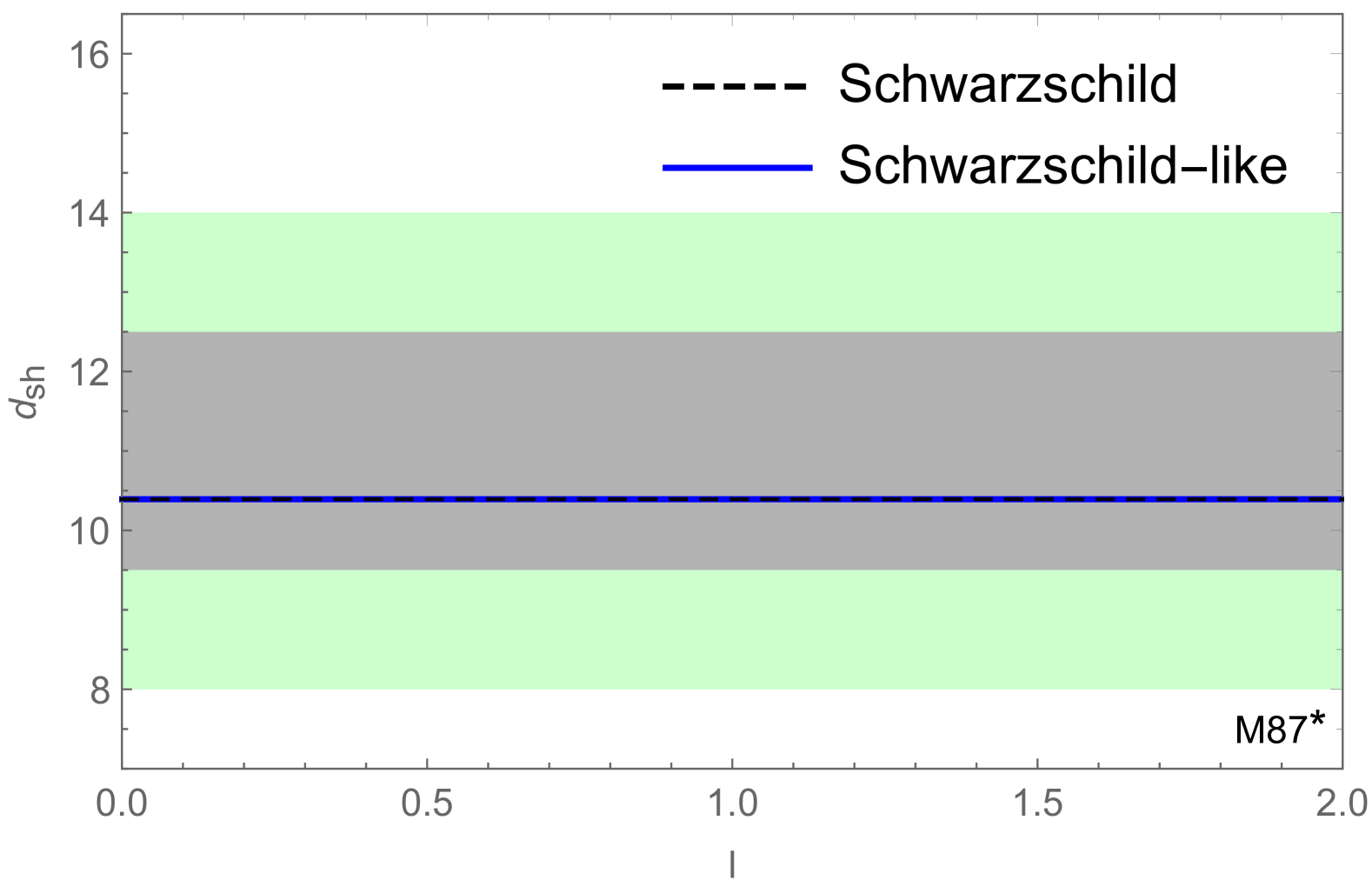
Figure 1: Shadow diameter of the Schwarzschild-like BH as a function of the parameter $l$.

Now let’s introduce a crucial concept, the innermost stable circular orbit (isco) of a time-like particle. The orbit equation of the time-like geodesic reads

$$\left(\frac{dr}{d\phi}\right)^{2}=\frac{r^{4}}{1+l}\left(\frac{1}{b^{2}}-\frac{f(r)}{r^{2}}-\frac{f(r)}{L^{2}}\right)=\tilde{V}_{eff}.$$ (26)

The radius $r_{isco}$ of the innermost stable circular orbit is given by

$$\tilde{V}_{eff}|_{r=r_{isco}}=\frac{d\tilde{V}_{eff}}{dr}|_{r=r_{isco}}=\frac{d^{2}\tilde{V}_{eff}}{dr^{2}}|_{r=r_{isco}}=0.$$ (27)

In the analysis of the image of thin accretion disks, the innermost stable circular orbit plays a crucial role as it defines the inner boundary of the disk. For radii $r<r_{isco}$, equatorial circular orbits become unstable, meaning that any perturbation will cause particles to either fall into the black hole or escape to greater distances. Thus, isco determines the inner edge of the accretion disk by marking the threshold at which orbits begin to destabilize. Specifically, isco signifies the critical boundary where internal orbits lose stability, thereby establishing the disk’s innermost extent.

II.3 Photon trajectory

In order to calculate the photon orbit, we introduce a new variable $u=1/r$, and the equation of motion for photon can be rewritten as

$$\left(\frac{du}{d\phi}\right)^{2}=\frac{1}{1+l}\left[\frac{1}{b^{2}}-u^{2}f(\frac{1}{u})\right]\equiv F(u).$$ (28)

We have plotted the $F(u)$ images with different parameters $l$ and shown in FIG. 2. It is shown that, as the value of parameter $l$ increases, the corresponding value of $F(u)$ decreases. When $b>b_{c}$, $F(u)$ has two roots; when $b=b_{c}$, $F(u)$ has one root; and when $b<b_{c}$, $F(u)$ has no roots.

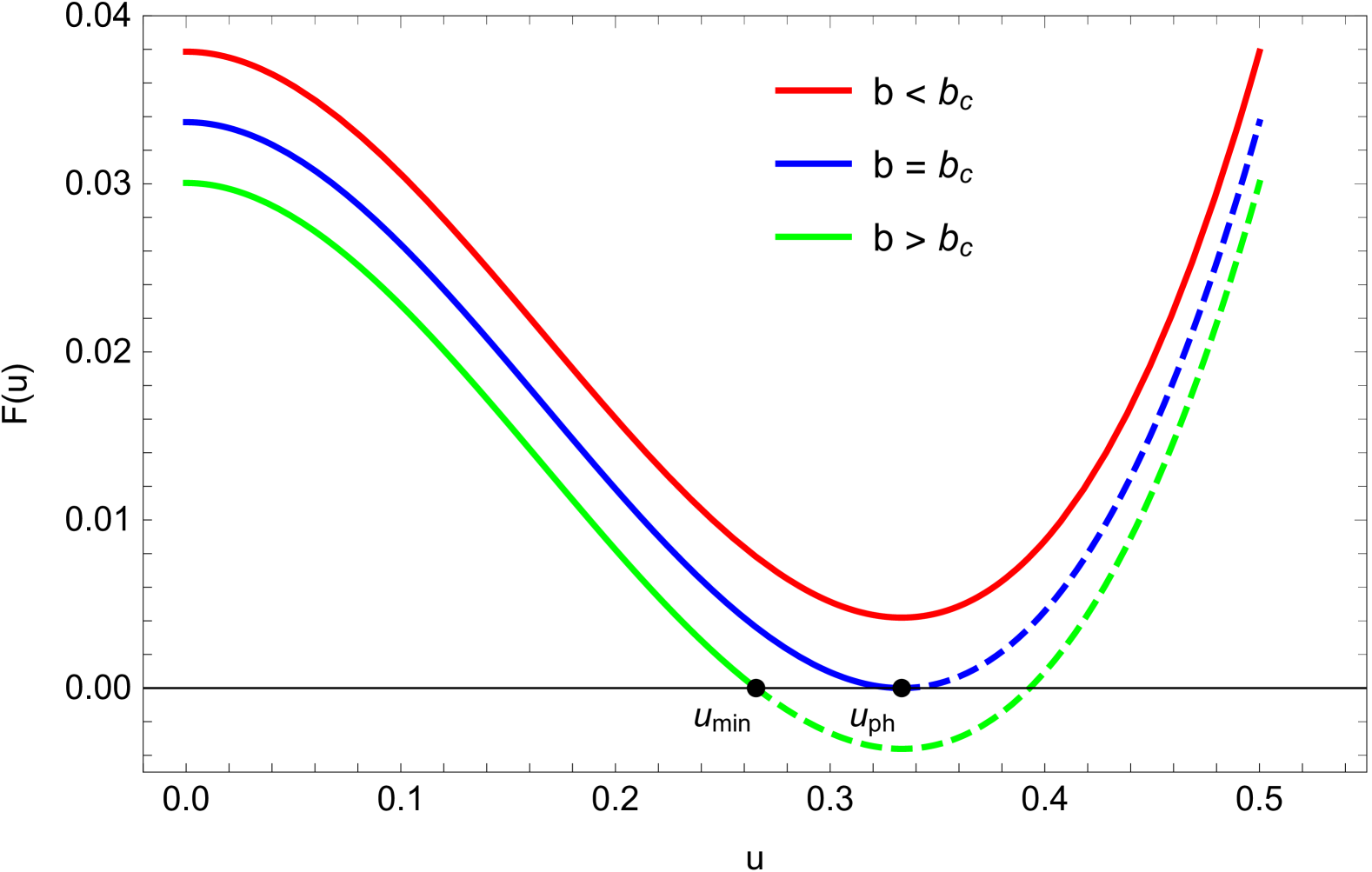
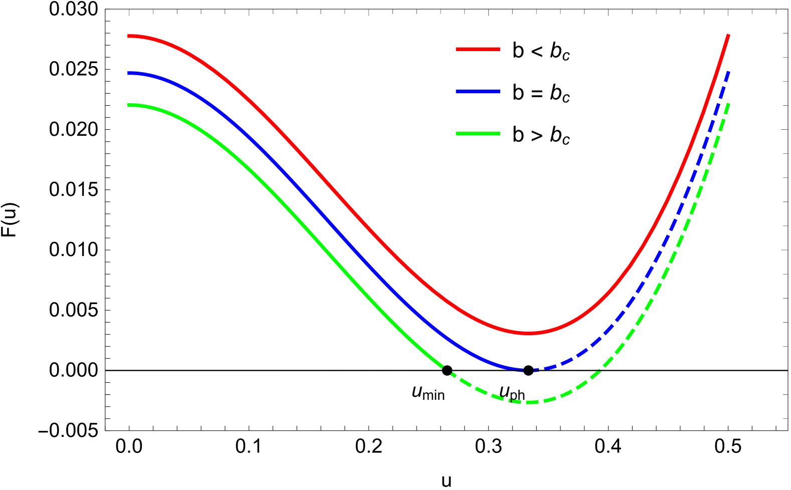
Figure 2: The functions $F(u)$ for different values of $l$, as a function of $u$. Left panel: $l=0.1$. Right panel: $l=0.5$. $u_{ph}=1/r_{ph}$, $u_{min}$ is the minimum positive root of F(u) when $b>b_{c}$.

In scenarios where $b<b_{c}$, our consideration is limited to the trajectory outside the event horizon, from which we derive the total change in the azimuthal angle $\varphi$ (We employ $\phi$ and $\varphi$ to represent the space-time coordinate and the change in $\phi$ associated with the photon’s motion, respectively):

$$\varphi=\int_{0}^{u_{h}}\frac{1}{\sqrt{F(u)}}du,\ b<b_{c}.$$ (29)

Here, $u_{h}=1/r_{h}$, where $r_{h}$ is the radius of the outermost horizon. In the case where $b>b_{c}$, the overall variation in the azimuthal angle $\varphi$ for a trajectory characterized by an impact parameter $b$ can be determined by

$$\varphi=2\int_{0}^{u_{min}}\frac{1}{\sqrt{F(u)}}du,\ b>b_{c},$$ (30)

where $u_{min}$ is the minimum positive root of $F(u)=0$ when $b>b_{c}$.

For a photon with an impact parameter $b=b_{c}$, it will reach $u_{ph}$ and subsequently engage in perpetual circular motion. We present the azimuthal angle $\varphi$ the image as a function of $b$ is shown in FIG. 3. It can be observed from the figure that $\varphi(b)=\pi$ is an asymptote of the graph. As $l$ increases, the entire graph of $\varphi(b)$ will shift downwards.

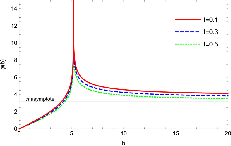
Figure 3: The azimuthal angle $\varphi(b)$ for different values of $l$, as a function of $b$.

At last, we plot the photon trajectories for different parameters as FIG. 4. The findings in FIG. 4 illustrates the trajectories of light near a black hole, with the gray line indicating cases where $\varphi<1.5\pi$, the orange line denoting scenarios where $1.5\pi<\varphi<2.5\pi$, and the red line representing the condition where $\varphi>2.5\pi$. Specifically, when $l$ is set to $-0.5$, the trajectory of light exhibits a repulsive effect by the black hole.

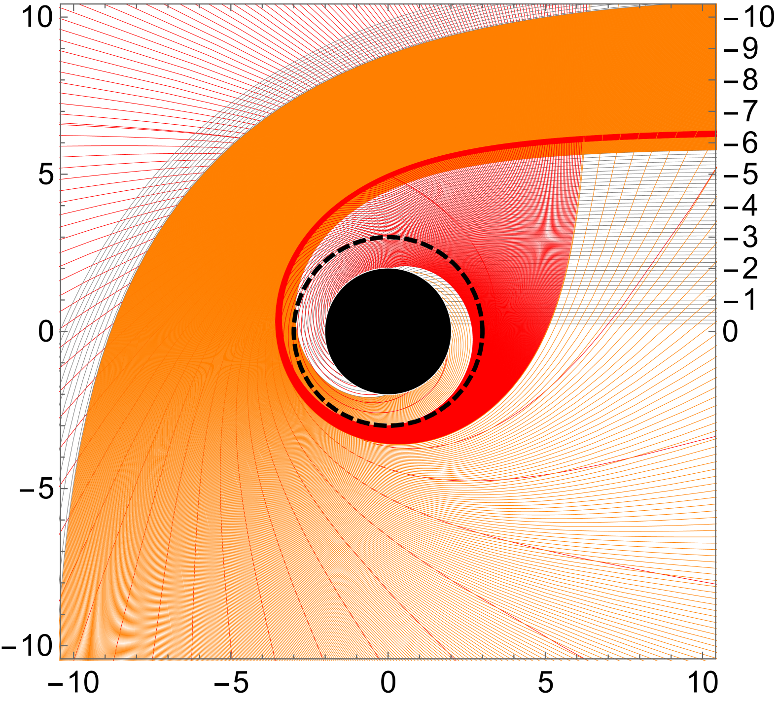
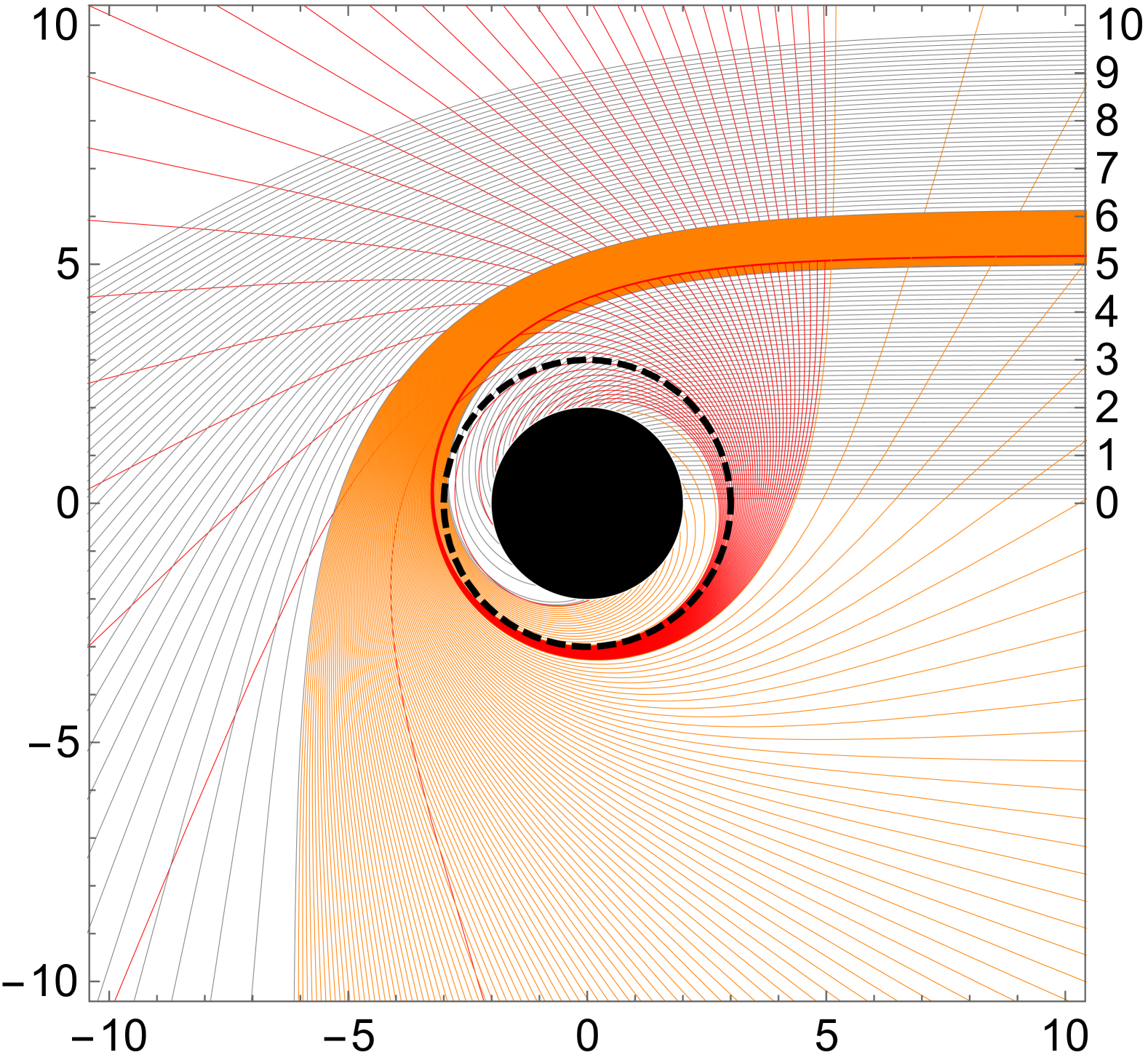
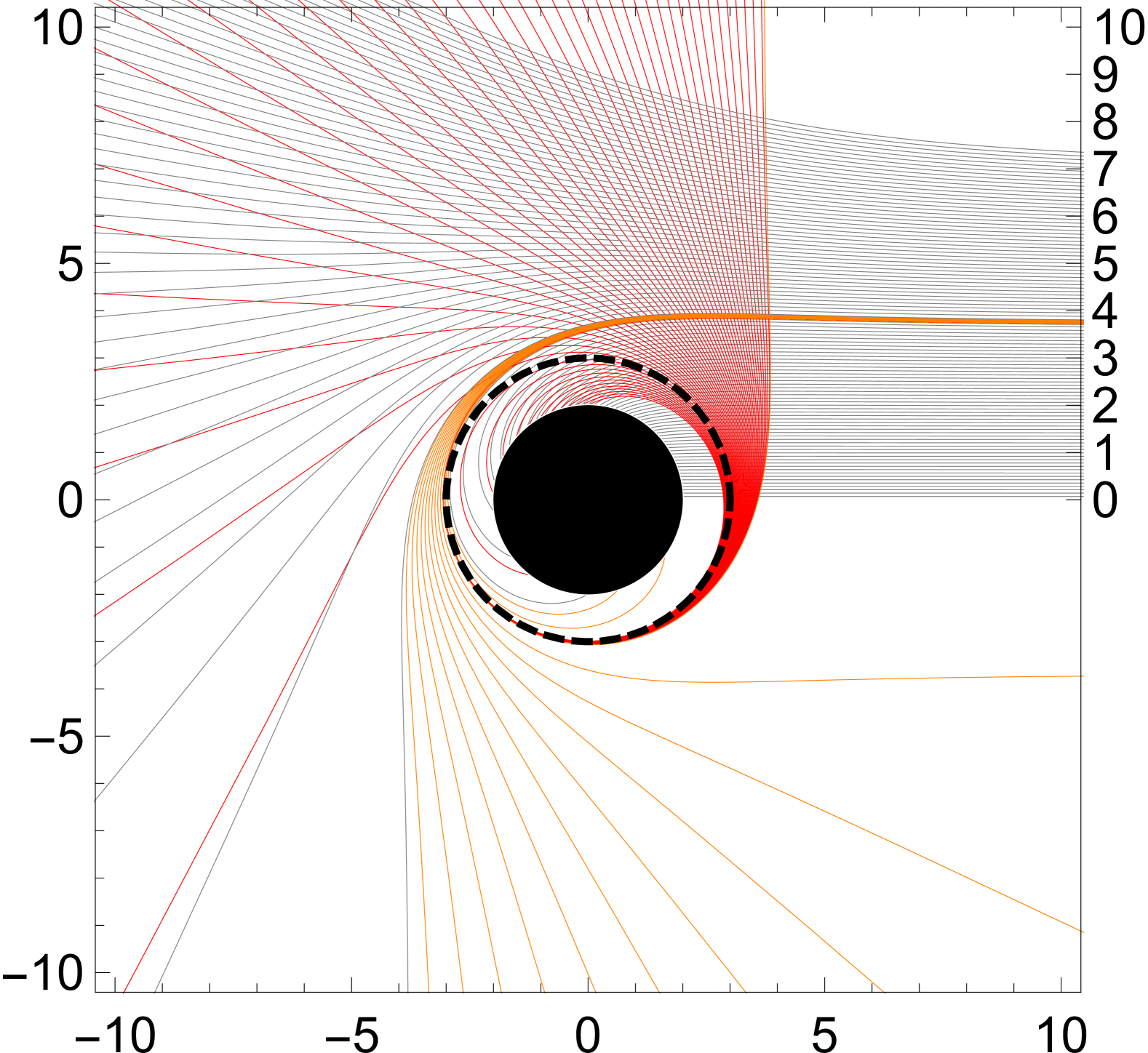
Figure 4: Photon trajectories at different $l$ values. Left panel: $l=0.5$. Middle panel: $l=0$. Right panel: $l=-0.5$.

III The properties of thin accretion disk

In this section, we will explore the accretion processes occurring in thin disks surrounding Schwarzschild-like BH. A detailed discussion will be provided on how the parameter $l$ affects the radiant energy flux, radiation temperature, and observable luminosity. The following values are adopted for the physical constants and the characteristics of the thin accretion disk in our analysis: $c=2.997\times 10^{10}cms^{-1}$, $\dot{M}_{0}=2\times 10^{-6}M_{\odot}yr^{-1}$, $1yr=3.156\times 10^{7}s$, $\sigma_{SB}=5.67\times 10^{-5}ergs^{-1}cm^{-2}K^{-4}$, $h=6.625\times 10^{-27}ergs$, $k_{B}=1.38\times 10^{-16}ergK^{-1}$, $M_{\odot}=1.989\times 10^{33}g$, and the mass of BH $M=2\times 10^{6}M_{\odot}$. The surface radiant energy flux is determined based on the methods outlined in Page:1974he

$$F(r)=-\frac{\dot{M}_{0}\Omega_{,r}}{4\pi\sqrt{-g}(E-\Omega L)^{2}}\int^{r}_{r_{isco}}(E-\Omega L)L_{,r}dr.$$ (31)

The equation is commonly used in the literature for cylindrical coordinates. However, for applications in spherical coordinates, it must be reformulated as detailed in Collodel:2021gxu .

$$F(r)=-\frac{-c^{2}\dot{M}_{0}\Omega_{,r}}{4\pi\sqrt{-g/g_{\theta\theta}}(E-\Omega L)^{2}}\int^{r}_{r_{isco}}(E-\Omega L)L_{,r}dr,$$ (32)

where $\dot{M}_{0}$ stands for the mass accretion rate, $g$ refers to the metric determinant. $E$, $L$, and $\Omega$ denote the energy, angular momentum, and angular velocity of the particle in the circular orbit, respectively. As shown in FIG. 5, the energy flux $F(r)$ of a disk around a Schwarzschild-like black hole varies with different values of $l$. The black line represents the energy flux of a Schwarzschild (Sch) BH. Regardless of whether $l$ is positive or negative, the energy flux decreases as $l$ increases. Moreover, the energy flux for negative $l$ values is higher compared to positive $l$ values. This observation can potentially assist in constraining the parameter $l$ using astronomical data. For a general static spherically symmetric metric $ds^{2}=g_{tt}dt^{2}+g_{rr}dr^{2}+g_{\theta\theta}d\theta^{2}+g_{\varphi\varphi}d\varphi^{2}$, $E$, $L$, and $\Omega$ are denoted as

$$E=-\frac{g_{tt}}{\sqrt{-g_{tt}-g_{\phi\phi}\Omega^{2}}},$$ (33)

$$L=\frac{g_{\phi\phi}\Omega}{\sqrt{-g_{tt}-g_{\phi\phi}\Omega^{2}}},$$ (34)

$$\Omega=\frac{d\phi}{dt}=\sqrt{-\frac{g_{tt,r}}{g_{\phi\phi,r}}}.$$ (35)

Within the Novikov-Thorne model framework, the accreted material reaches a state of thermodynamic equilibrium, which implies that the radiation emitted by the disk closely resembles that of a perfect black body. The relationship between the disk’s radiation temperature $T(r)$ and its energy flux $F(r)$ is given by the Stefan-Boltzmann law: $F(r)=\sigma_{SB}T^{4}(r)$, where $\sigma_{SB}$ represents the Stefan-Boltzmann constant. In FIG. 6, we present the radiation temperature $T(r)$) for the region surrounding a Schwarzschild-like black hole. Regardless of whether $l$ is positive or negative, the radiation temperature $T(r)$ decreases as the magnitude of the parameter $l$ increases.

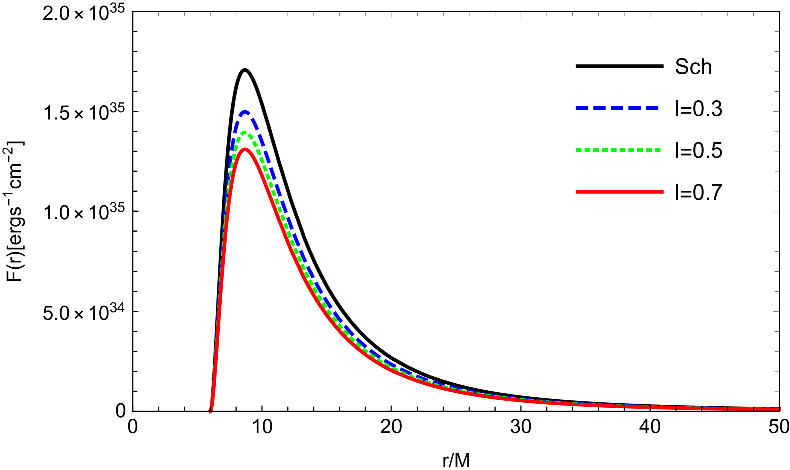
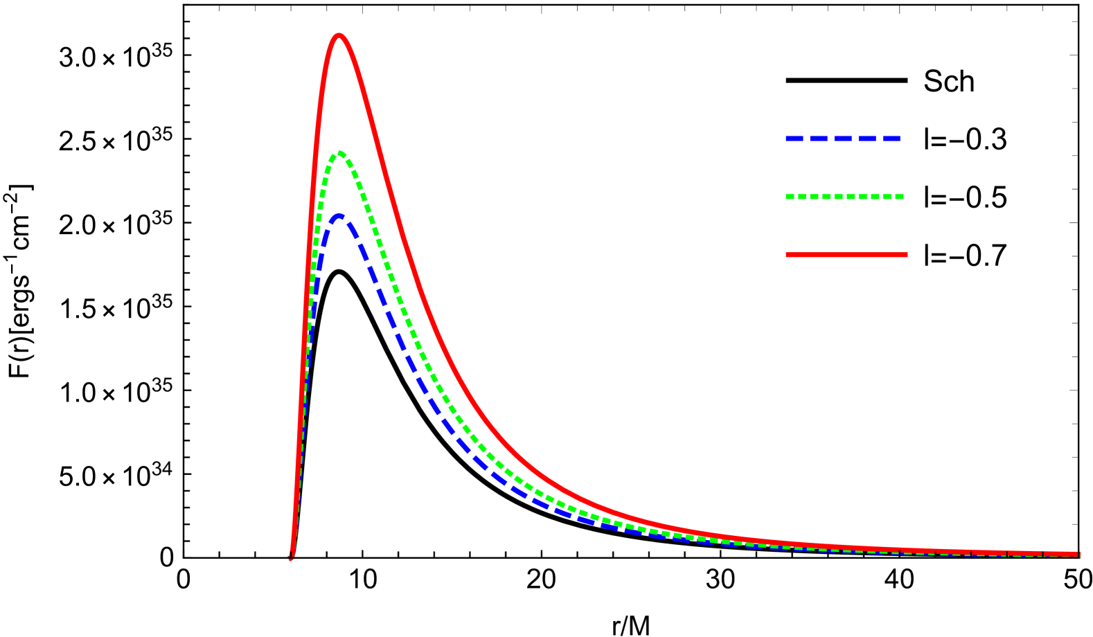
Figure 5: The energy flux $F(r)$ from a disk around a Schwarzschild-like BH in bumblebee gravity for different values of $l$.

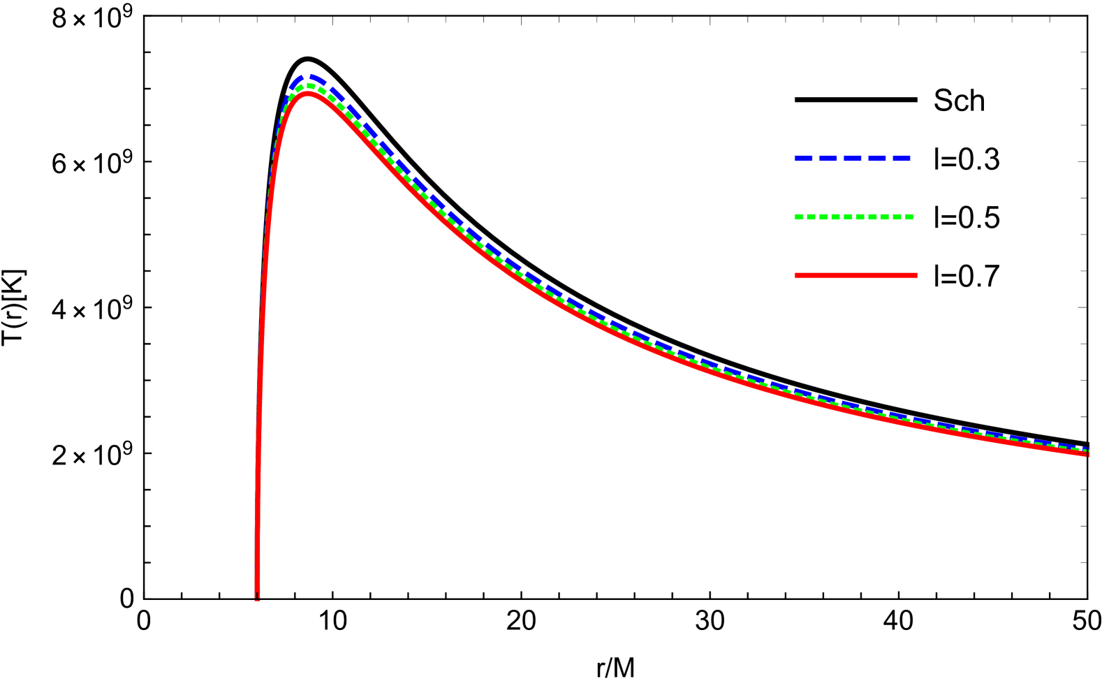
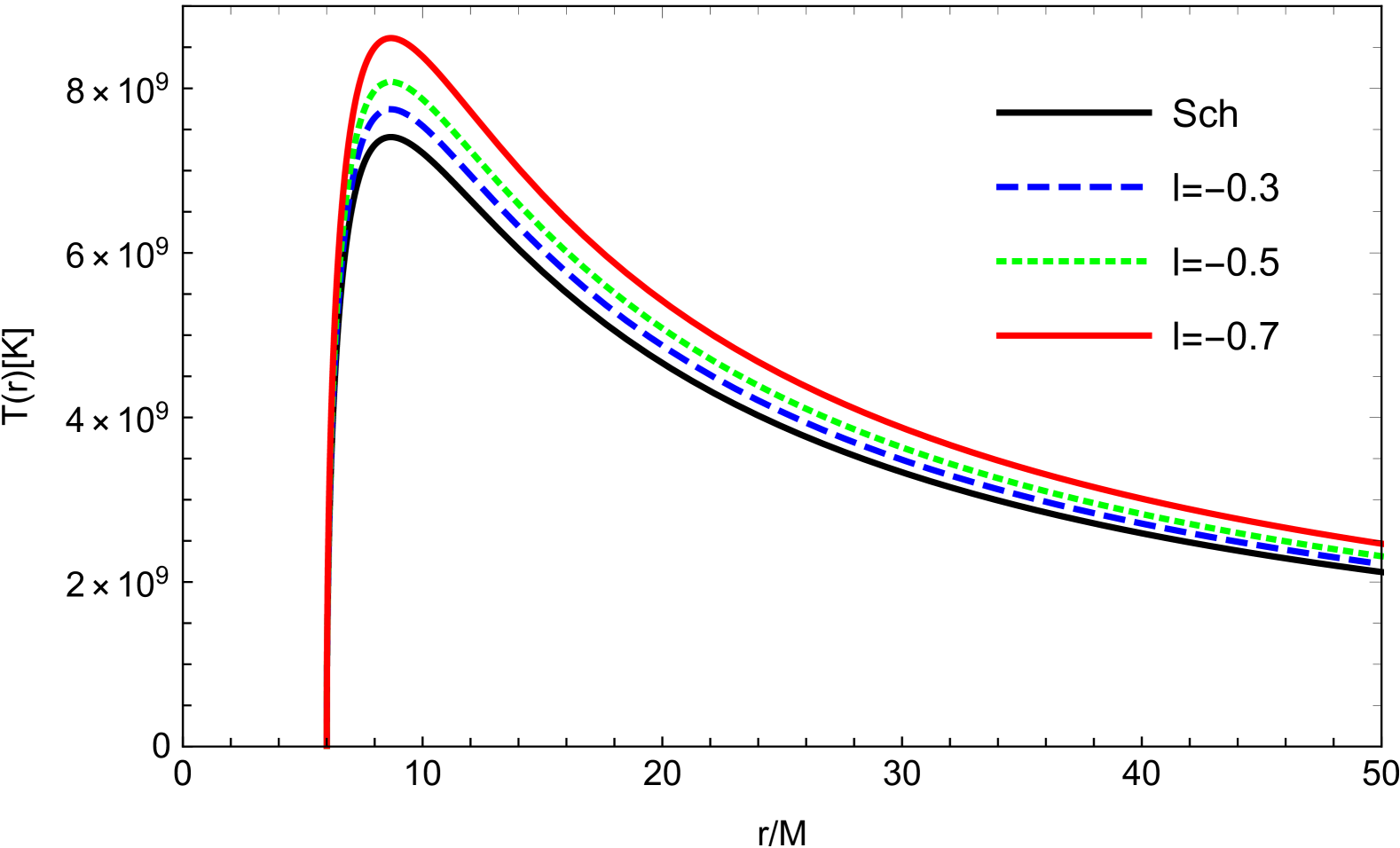
Figure 6: Variety of the disk temperature $T(r)$ with different parameters $l$ for the thin disk around a Schwarzschild-like BH in bumblebee gravity.

The red-shifted black body spectrum of the observed luminosity $L(\nu)$ for a thin accretion disk around a black hole is provided in Torres:2002td .

$$L(\nu)=4\pi d^{2}I(\nu)=\frac{8\pi h\cos\theta}{c^{2}}\int_{r_{i}}^{r_{f}}\int_{0}^{2\pi}\frac{\nu_{e}^{3}r}{e^{\frac{h\nu_{e}}{k_{B}T}}-1}drd\phi,$$ (36)

where, $d$ represents the distance to the disk center, $I(\nu)$ denotes the thermal energy flux radiated by the disk, $h$ is the Planck constant, $k_{B}$ is the Boltzmann constant, and $\theta$ is the disk inclination angle, which we will set to zero. The quantities $r_{f}$ and $r_{i}$ correspond to the outer and inner radii of the disk’s edges, respectively. Assuming that the flux over the disk surface approaches zero, we select $r_{i}=r_{isco}$ and $r_{f}\rightarrow\infty$ for calculating the luminosity $L(\nu)$ of the disk. The emitted frequency is given by $\nu_{e}=\nu(1+z)$, where the redshift factor $z$ can be expressed as follows Luminet:1979nyg :

$$1+z=\frac{1+\Omega b\sin\theta\cos\alpha}{\sqrt{-g_{tt}-g_{\phi\phi}\Omega^{2}}}.$$ (37)

In this case, we designate $\alpha$ from equation (17) in reference Luminet:1979nyg as $\alpha^{\prime}$. The relationship between $\alpha$ and $\alpha^{\prime}$ is defined by $\alpha=\frac{\pi}{2}-\alpha^{\prime}$. For the sake of illustration and simplicity in calculations, we neglect light bending Bhattacharyya:2000kt . We thus write $b\cos\alpha=r\sin\phi$ and the redshift factor $z$ can be rewritten as:

$$1+z=\frac{1+\Omega r\sin\theta\sin\phi}{\sqrt{-g_{tt}-g_{\phi\phi}\Omega^{2}}}.$$ (38)

FIG. 7 presents the variations observed in the spectral energy distribution. Following the same pattern as seen with the energy flux and disk temperature, we observe that for negative $l$, the disk around a Schwarzschild-like BH is more luminous than one around a Schwarzschild BH in GR. On the other hand, for positive $l$, the disk is less luminous.

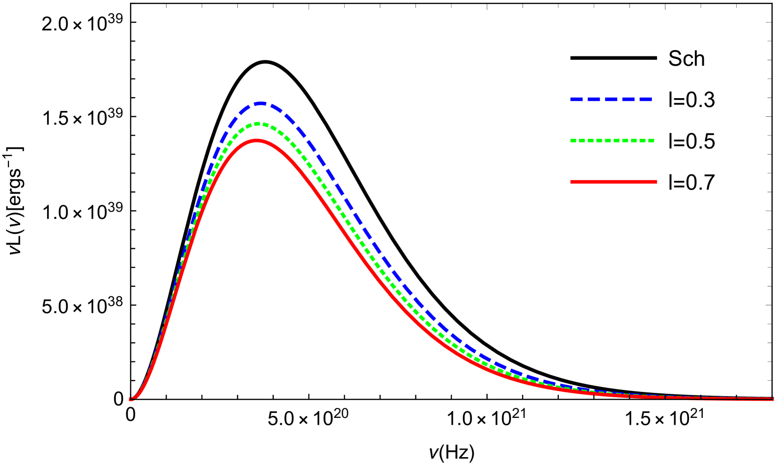
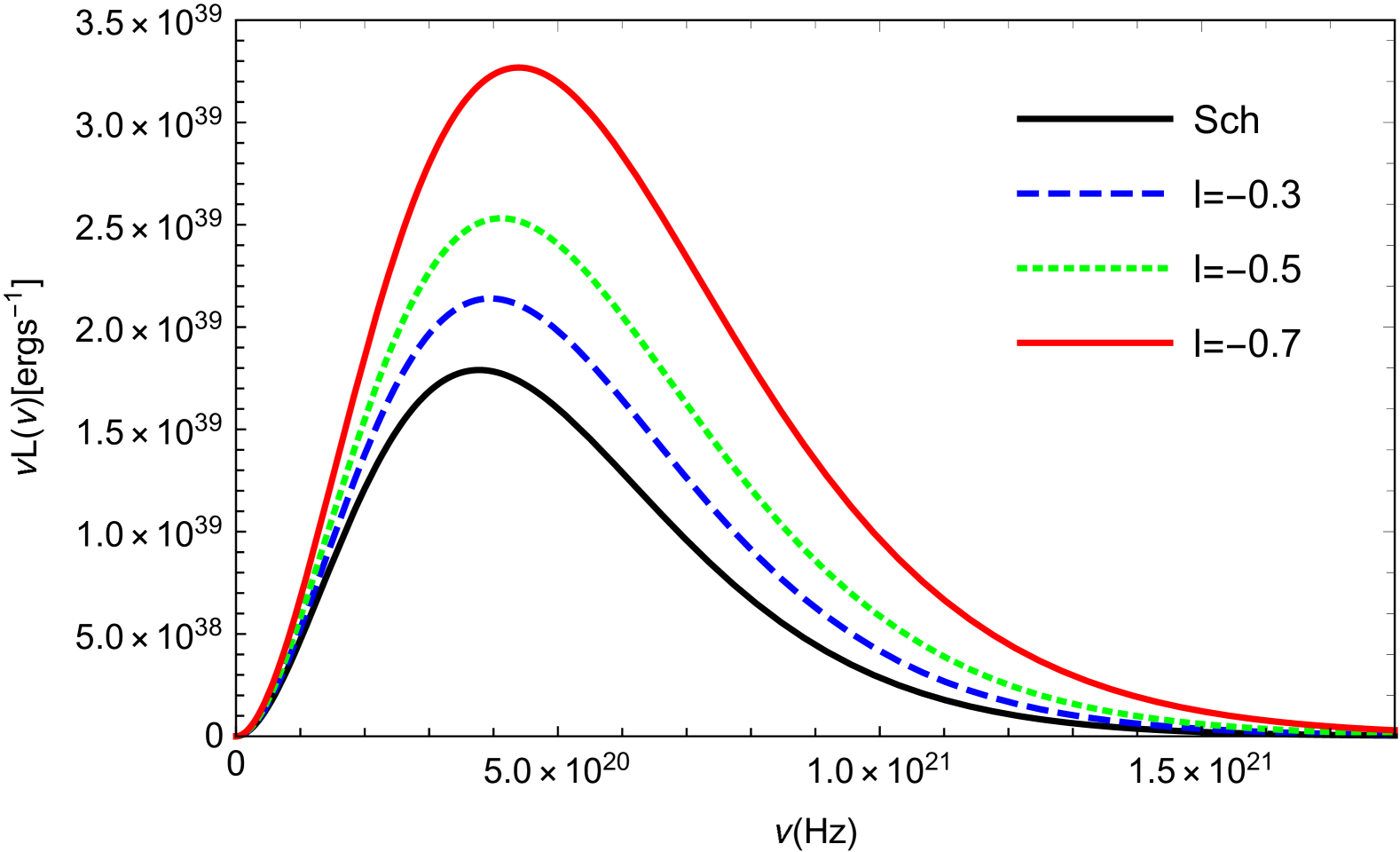
Figure 7: The emission spectrum $\nu L(\nu)$ of the accretion disk around a Schwarzschild-like BH in bumblebee gravity for different values of $l$, as a function of frequency $\nu$.

IV Image of the thin accretion disk around Schwarzschild-like BHs

IV.1 The image and coordinate system of the thin accretion disk

To analyze the imaging of a thin accretion disk, we employ an observational coordinate system as illustrated in FIG. 8. The observer is positioned at $(\infty,\theta,0)$ within the BH’s spherical coordinate system $(r,\theta,\phi)$, with the origin at the BH’s center $(r=0)$.

In this observer-based $O^{\prime}X^{\prime}Y^{\prime}$ coordinate system, consider a photon that originates from point $q(b,\alpha)$ and travels vertically. Here, $b$ represents the photon’s impact parameter. This photon intersects the accretion disk at point $Q(r,\frac{\pi}{2},\phi)$. By applying the principle of optical path reversibility, a photon emitted from $Q(r,\frac{\pi}{2},\phi)$ within the accretion disk will follow a trajectory that ultimately reaches the image point $q(b,\alpha)$ in the observer’s field of view.

When the radial distance $r$ is held constant, the resulting image corresponds to an orbit of constant radius. As depicted on the left side of FIG. 8, every $\alpha/\alpha+\pi$ plane intersects the constant-$r$ orbit within the equatorial plane at two distinct points, with their azimuthal angles $\phi$ differing by $\pi$. For our coordinate system, the $X^{\prime}$-axis is defined by setting $\alpha=0$, while the $X$-axis is aligned with $\phi=0$. Geometrically, this setup allows us to determine the angle $\varphi$ formed between the rotational axis and the line segment $OQ$

$$\varphi=\frac{\pi}{2}+\arctan(\tan\theta\sin\alpha).$$ (39)

As the impact parameter $b$ approaches $b_{c}$, the degree of light bending increases, potentially causing a single source point $Q$ to produce multiple image points $q$. These image points are labeled according to their increasing azimuthal angles $\varphi$ as $q^{n}$ $(n\in\mathbb{N})$, where $n$ denotes the order of the image.

As illustrated in FIG. 8 (right side), all even-order images of $Q$ appear on the same side $(\alpha)$ as the source point $Q$, while all odd-order images are located on the opposite side $(\alpha+\pi)$. The angular deflections responsible for generating the $n^{th}$-order image are denoted by $\varphi^{n}$

$$\varphi^{n}=\begin{cases}\frac{n}{2}2\pi+(-1)^{n}[\frac{\pi}{2}+\arctan(\tan\theta\sin\alpha)],&\text{when $n$ is even,}\\ \frac{n+1}{2}2\pi+(-1)^{n}[\frac{\pi}{2}+\arctan(\tan\theta\sin\alpha)],&\text{when $n$ is odd,}\end{cases}$$ (40)

the parameter $n$ denotes the order of the image observed. Specifically, when $n=0$, it corresponds to the primary, or direct, visualization of the accretion disk as seen by an observer. Higher values of $n$, such as 1, 2, 3, and so forth, indicate successive orders of images, capturing secondary, tertiary, and further iterative representations, respectively.

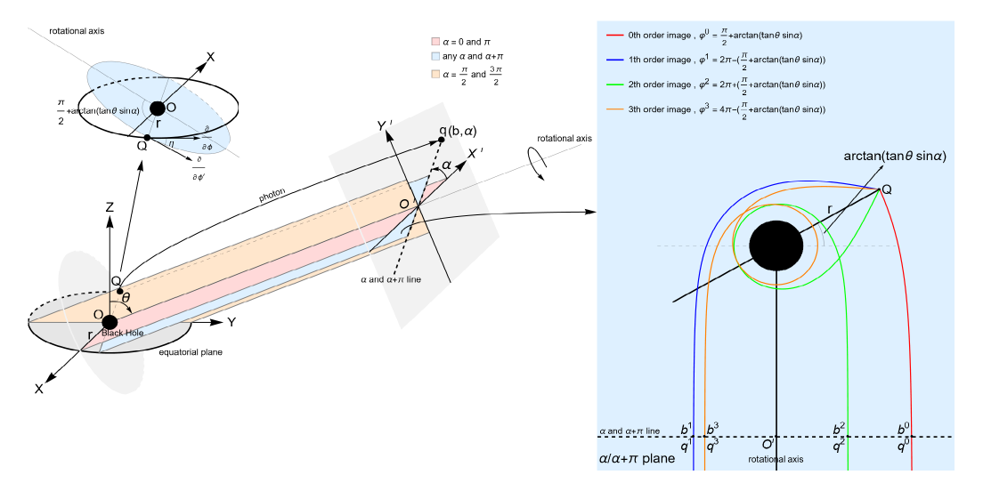
Figure 8: Coordinate system is indicated in Ref.You:2024uql .

IV.2 Image of equal-$r$ orbit on thin accretion disk

Photons arriving from infinity with varying impact parameters $b$ intersect the equal-$r$ orbit at different points. FIG. 9 depicts the function $\varphi(b)$. As can be seen from the figure, as $l$ increases, the graph of $\varphi(b)$ shifts upward. The purple dashed line in the figure is designated as $\varphi_{1}(b)$. Taking this line as a dividing boundary, the colored curves lying below it are denoted as $\varphi_{2}(b)$, while those above it are labeled as $\varphi_{3}(b)$. Therefore, we can define:

$$\varphi_{1}(b)=\int_{0}^{u_{min}}\frac{1}{\sqrt{F(u)}}du,$$ (41)

$$\varphi_{2}(b)=2\int_{0}^{u_{r}}\frac{1}{\sqrt{F(u)}}du,$$ (42)

$$\varphi_{3}(b)=2\int_{0}^{u_{min}}\frac{1}{\sqrt{F(u)}}du-\int_{0}^{u_{r}}\frac{1}{\sqrt{F(u)}}du.$$ (43)

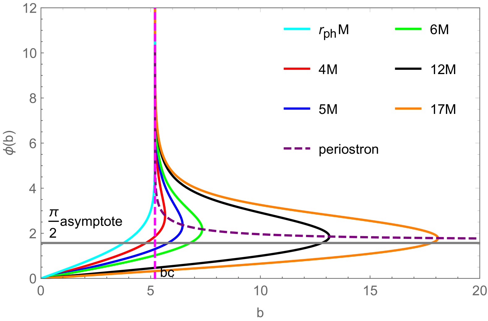
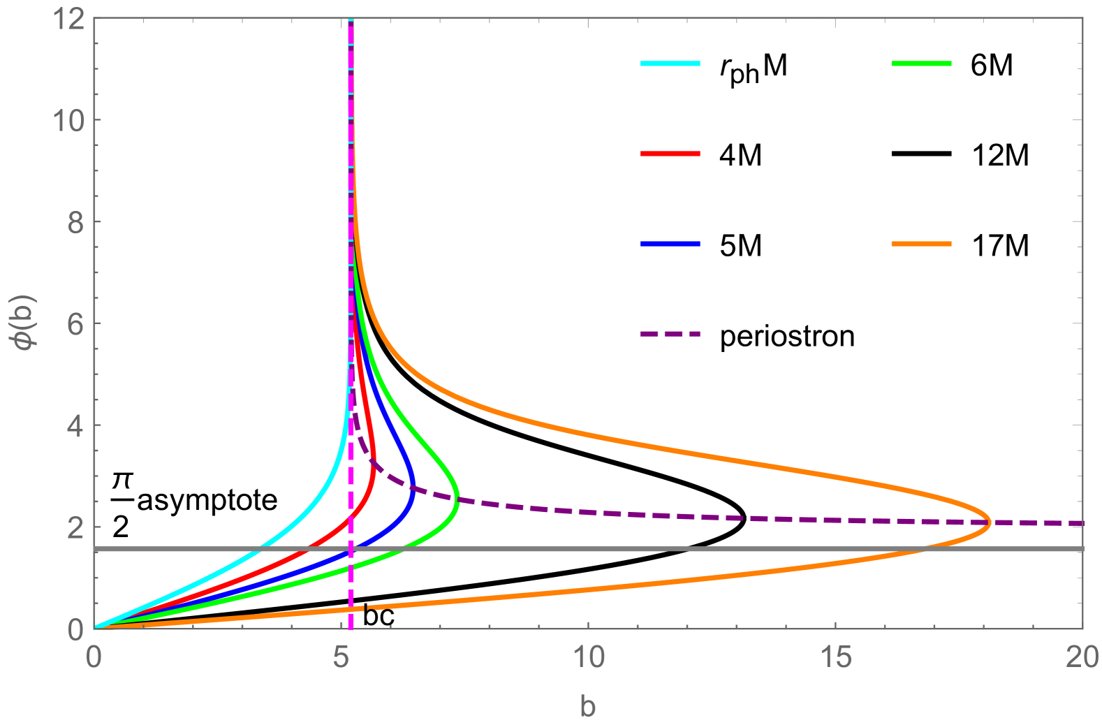
Figure 9: Deflection angle $\varphi(b)$ corresponding to intersections as a function of $b$ for different $r$. Left panel: $l=0.1$. Right panel: $l=0.5$.

Each colored curve in the figures denotes an equal-$r$ orbit, with points $(b,\varphi)$ indicating the deflection angle $\varphi$ for photons arriving at the equal-$r$ orbit with impact parameter $b$. The purple dashed line intersects these curves at their peak points, representing the deflection angle when photons reach their closest approach perihelion $r_{pe}$. It is evident that the purple dashed line asymptotically tends toward $\varphi=\frac{\pi}{2}$, corresponding to the case where photons with infinitely large impact parameters $b=\infty$ follow straight paths that are tangent to the circle at $r=\infty$ at $\varphi=\frac{\pi}{2}$.

By solving the system of equations (39), (41), and (42) simultaneously and employing numerical integration methods to find all $(b,\alpha)$ pairs, one can obtain the projection of the accretion disk in the observer’s plane.

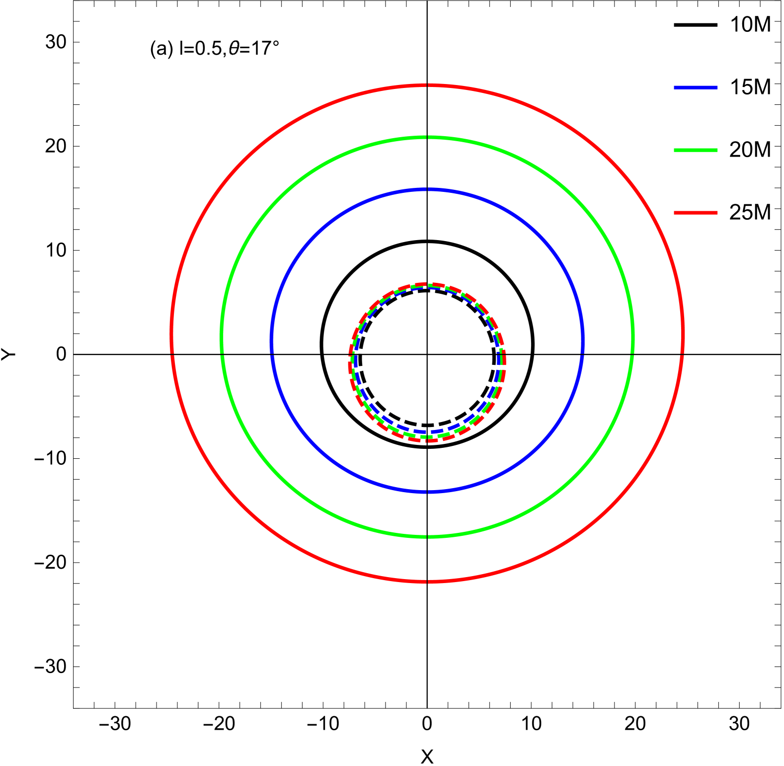
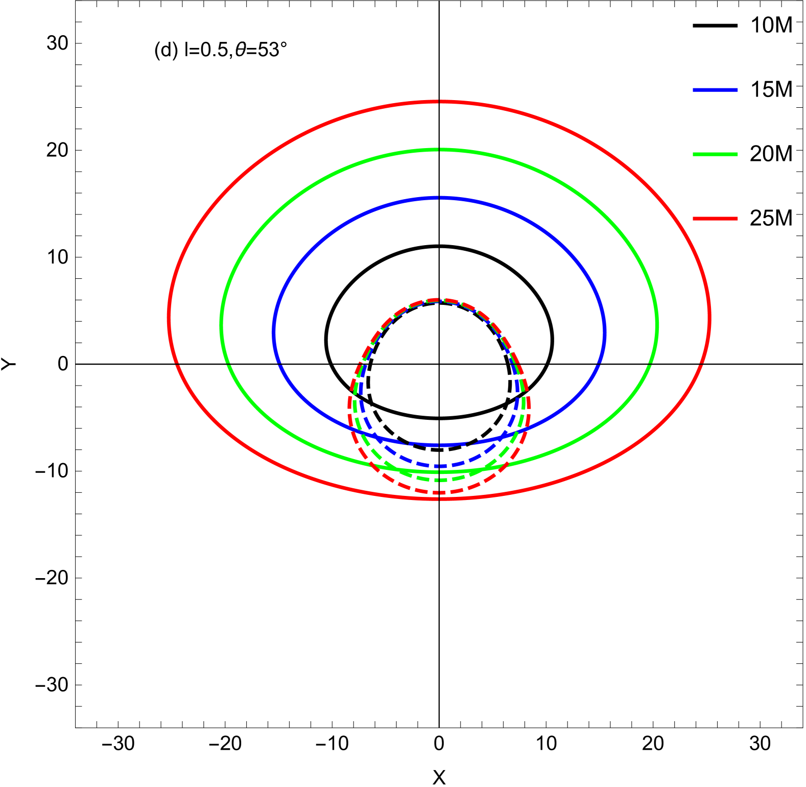
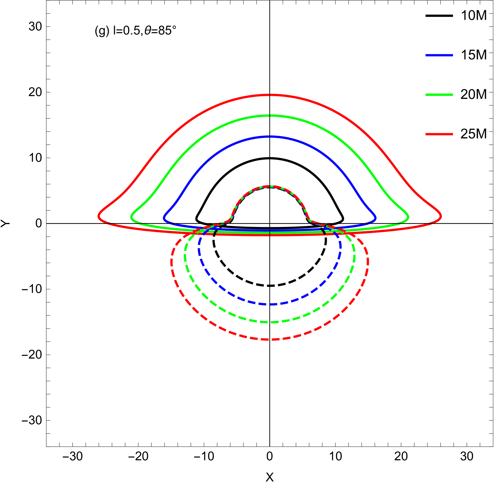
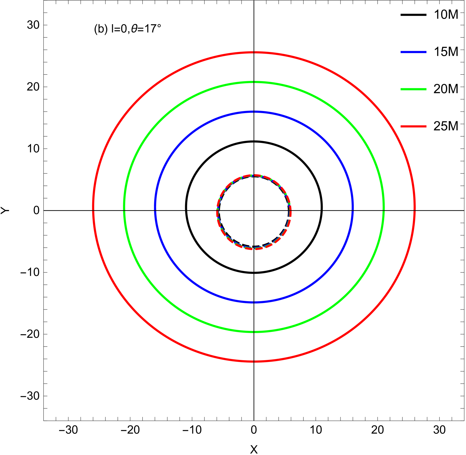
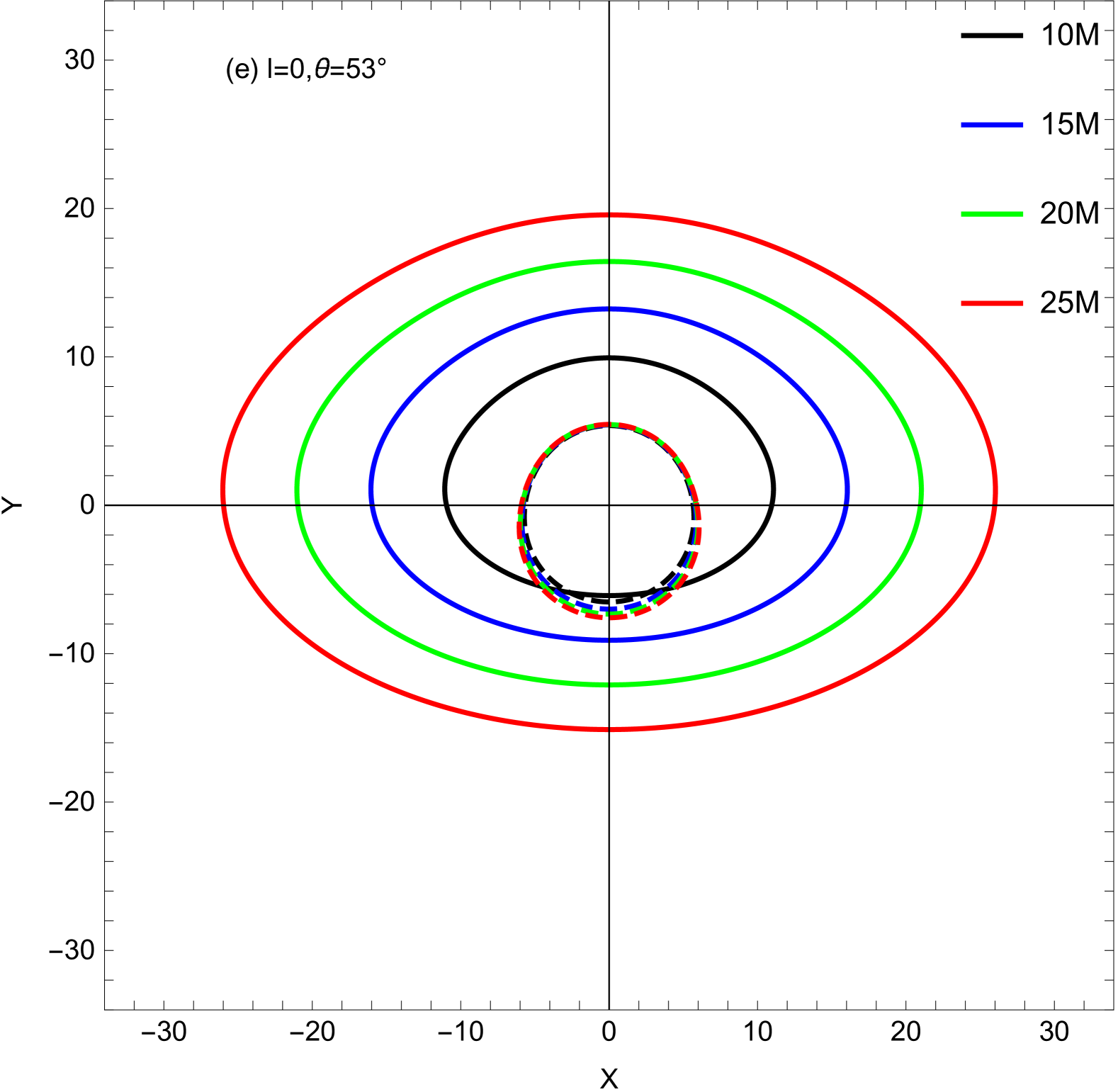
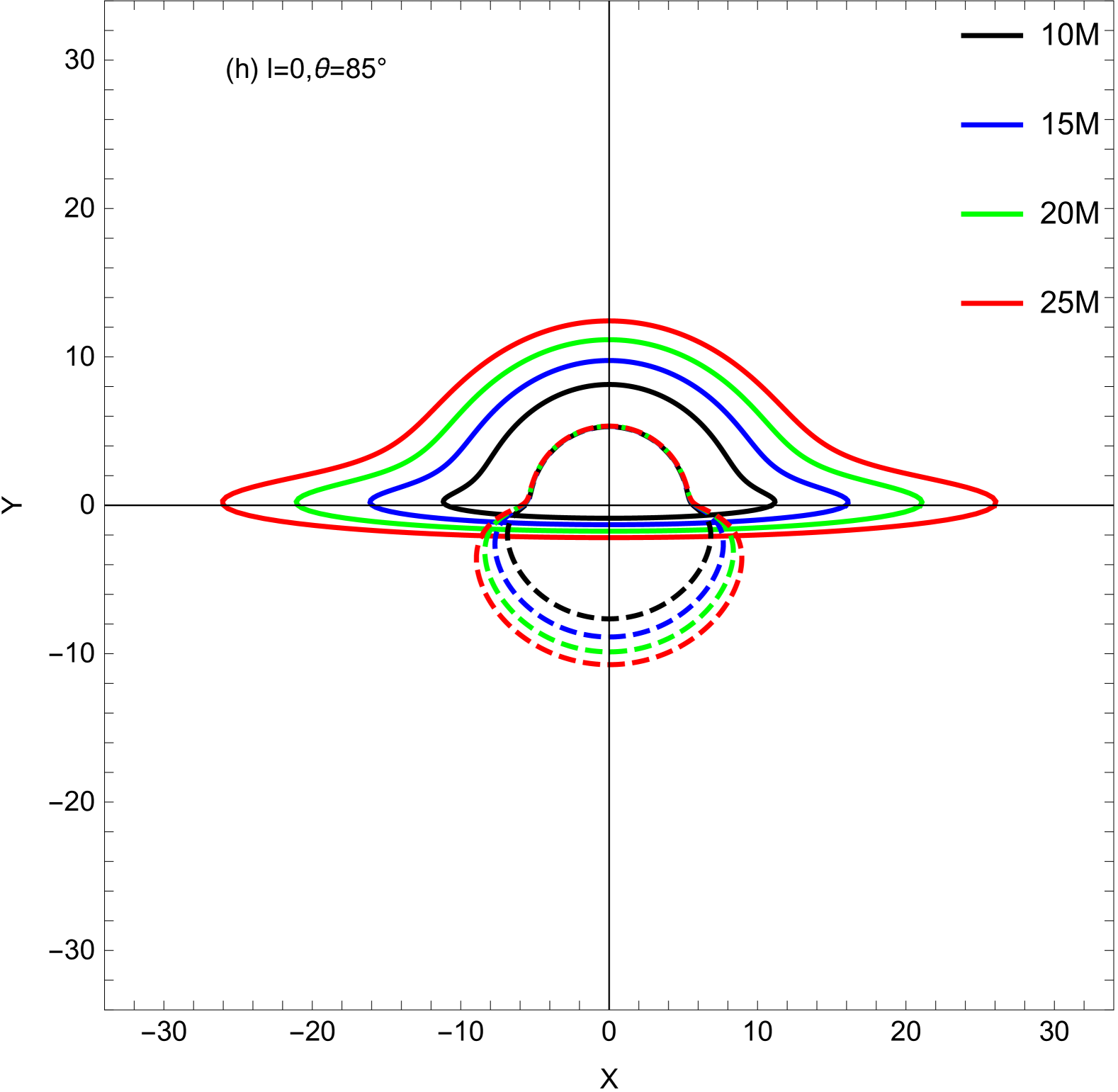
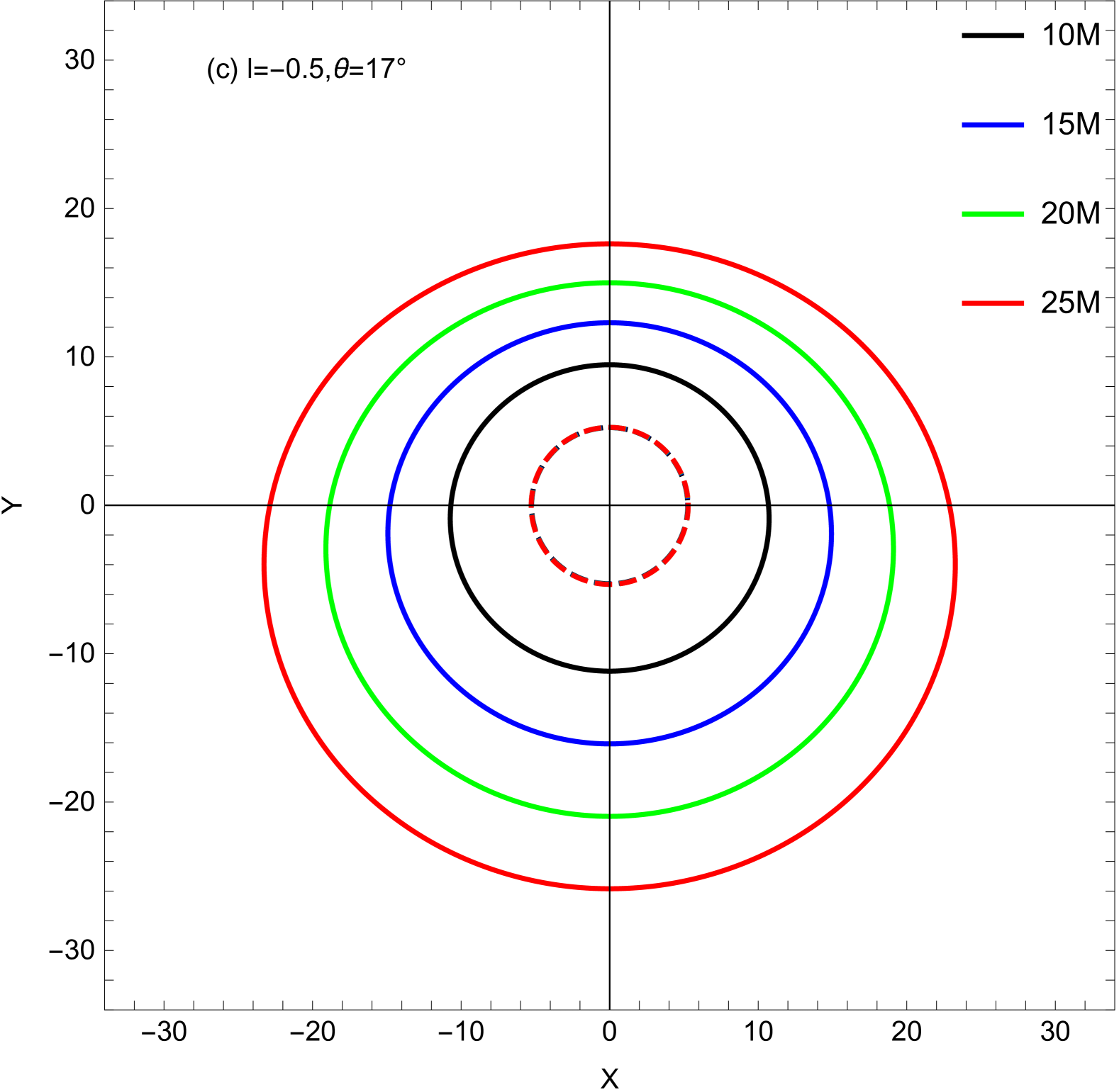
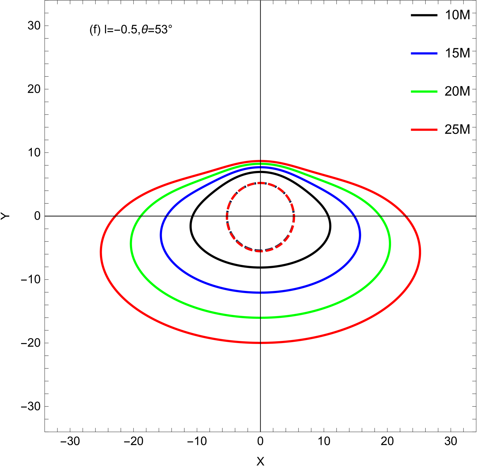
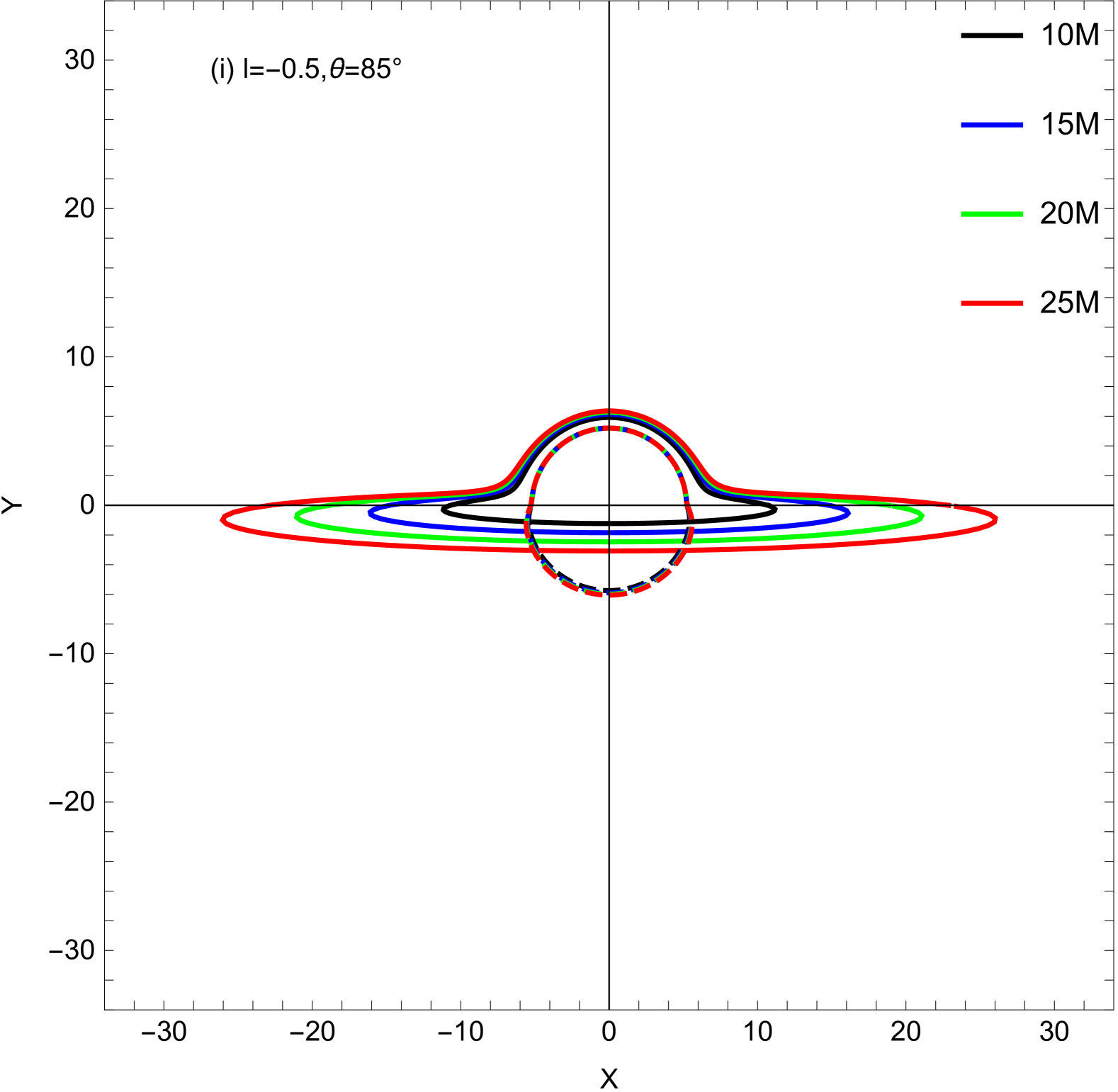
Figure 10: Direct and secondary image of the thin accretion disk.

FIG. 10 displays the direct and secondary images of representative stable circular orbits around Schwarzschild-like BHs, observed by a remote observer at various inclination angles. Each column, from top to bottom, corresponds to inclination angles of $17^{\circ}$, $53^{\circ}$, and $85^{\circ}$, while each row, from left to right, represents $l$ values of $0.5$, $0$, and $-0.5$, respectively. These images correspond to stable circular orbits with radii of $r=10$, 15, 20, 25, moving from the innermost to the outermost. The middle column corresponds to the Schwarzschild BH. Compared to the Schwarzschild BH, as $l$ increases, the cap shape contracts inward, whereas with decreasing $l$, the cap shape stretches outward.

IV.3 Observed Flux

To obtain the observable flux $F_{obs}$ at a specified point on the celestial sphere, the gravitational redshift $z$ must be taken into account. Therefore, we arrive at the relation:

$$F_{obs}=\frac{F(r)}{(1+z)^{4}}.$$ (44)

From Eqs. (31), (37), and (44), it follows that,

$$F_{obs}=\frac{-\frac{\dot{M}\Omega_{,r}}{4\pi\sqrt{-g}(E-\Omega L)^{2}}\int^{r}_{r_{isco}}(E-\Omega L)L_{,r}dr}{(\frac{1+\Omega b\sin\theta\cos\alpha}{\sqrt{-g_{tt}-g_{\phi\phi}\Omega^{2}}})^{4}}.$$ (45)

According to the analysis above, we plotted the observed flux distribution of the accretion disk as FIG. 11. Each column, from top to bottom, corresponds to inclination angles of $17^{\circ}$, $53^{\circ}$, and $85^{\circ}$, while each row, from left to right, represents $l$ values of $0.5$, $0$, and $-0.5$, respectively. The middle column corresponds to the Schwarzschild BH. As the observer’s inclination angle increases, the flux distributions become strongly asymmetric, and the brightness distribution patterns are similar.

\begin{overpic}[width=325.215pt]{actual_disk_image1.pdf} \put(20.0,103.0){\color[rgb]{0,0,0}\large$l=0.5,\theta=17^{\circ}$} \put(-10.0,48.0){\color[rgb]{0,0,0} Y} \put(48.0,-10.0){\color[rgb]{0,0,0} X} \end{overpic}	\begin{overpic}[width=325.215pt]{actual_disk_image2.pdf} \put(23.0,103.0){\color[rgb]{0,0,0}\large$l=0,\theta=17^{\circ}$} \put(-10.0,48.0){\color[rgb]{0,0,0} Y} \put(48.0,-10.0){\color[rgb]{0,0,0} X} \end{overpic}	\begin{overpic}[width=325.215pt]{actual_disk_image3.pdf} \put(14.0,103.0){\color[rgb]{0,0,0}\large$l=-0.5,\theta=17^{\circ}$} \put(-10.0,48.0){\color[rgb]{0,0,0} Y} \put(48.0,-10.0){\color[rgb]{0,0,0} X} \end{overpic}
\begin{overpic}[width=325.215pt]{actual_disk_image4.pdf} \put(20.0,103.0){\color[rgb]{0,0,0}\large$l=0.5,\theta=53^{\circ}$} \put(-10.0,48.0){\color[rgb]{0,0,0} Y} \put(48.0,-10.0){\color[rgb]{0,0,0} X} \end{overpic}	\begin{overpic}[width=325.215pt]{actual_disk_image5.pdf} \put(23.0,103.0){\color[rgb]{0,0,0}\large$l=0,\theta=53^{\circ}$} \put(-10.0,48.0){\color[rgb]{0,0,0} Y} \put(48.0,-10.0){\color[rgb]{0,0,0} X} \end{overpic}	\begin{overpic}[width=325.215pt]{actual_disk_image6.pdf} \put(14.0,103.0){\color[rgb]{0,0,0}\large$l=-0.5,\theta=53^{\circ}$} \put(-10.0,48.0){\color[rgb]{0,0,0} Y} \put(48.0,-10.0){\color[rgb]{0,0,0} X} \end{overpic}
\begin{overpic}[width=325.215pt]{actual_disk_image7.pdf} \put(20.0,103.0){\color[rgb]{0,0,0}\large$l=0.5,\theta=85^{\circ}$} \put(-10.0,48.0){\color[rgb]{0,0,0} Y} \put(48.0,-10.0){\color[rgb]{0,0,0} X} \end{overpic}	\begin{overpic}[width=325.215pt]{actual_disk_image8.pdf} \put(23.0,103.0){\color[rgb]{0,0,0}\large$l=0,\theta=85^{\circ}$} \put(-10.0,48.0){\color[rgb]{0,0,0} Y} \put(48.0,-10.0){\color[rgb]{0,0,0} X} \end{overpic}	\begin{overpic}[width=325.215pt]{actual_disk_image9.pdf} \put(14.0,103.0){\color[rgb]{0,0,0}\large$l=-0.5,\theta=85^{\circ}$} \put(-10.0,48.0){\color[rgb]{0,0,0} Y} \put(48.0,-10.0){\color[rgb]{0,0,0} X} \end{overpic}

Figure 11: The complete apparent images of the thin accretion disk for different values of parameter $l$ and inclination angle.

We investigate the redshift distributions (contour map of redshift z) in the direct images for various inclination angles and parameter $l$,as demonstrated in FIG. 12. The dependency of the redshift on parameter $l$ is also shown in the secondary images, which are plotted in FIG. 13. For high inclination angles, the blueshift $(z<0)$ in the left half of the plate exceeds the gravitational redshift $(z>0)$ due to the presence of the BH. Conversely, for low inclination angles, no blueshift distribution is observed. Additionally, we find that the region with high redshift values $z$ increases as the parameter $l$ decreases.

\begin{overpic}[width=325.215pt]{z_direct_image1.pdf} \put(20.0,100.0){\color[rgb]{0,0,0}\large$l=0.5,\theta=17^{\circ}$} \put(-8.0,48.0){\color[rgb]{0,0,0} Y} \put(48.0,-10.0){\color[rgb]{0,0,0} X} \end{overpic} \begin{overpic}[width=30.35657pt]{z_direct_image1_1.pdf} \put(0.0,103.0){\color[rgb]{0,0,0}\large$z$} \end{overpic}	\begin{overpic}[width=325.215pt]{z_direct_image2.pdf} \put(28.0,100.0){\color[rgb]{0,0,0}\large$l=0,\theta=17^{\circ}$} \put(-8.0,48.0){\color[rgb]{0,0,0} Y} \put(48.0,-10.0){\color[rgb]{0,0,0} X} \end{overpic} \begin{overpic}[width=30.35657pt]{z_direct_image2_1.pdf} \put(0.0,103.0){\color[rgb]{0,0,0}\large$z$} \end{overpic}	\begin{overpic}[width=325.215pt]{z_direct_image3.pdf} \put(15.0,100.0){\color[rgb]{0,0,0}\large$l=-0.5,\theta=17^{\circ}$} \put(-8.0,48.0){\color[rgb]{0,0,0} Y} \put(48.0,-10.0){\color[rgb]{0,0,0} X} \end{overpic} \begin{overpic}[width=30.35657pt]{z_direct_image3_1.pdf} \put(0.0,103.0){\color[rgb]{0,0,0}\large$z$} \end{overpic}
\begin{overpic}[width=325.215pt]{z_direct_image4.pdf} \put(20.0,100.0){\color[rgb]{0,0,0}\large$l=0.5,\theta=53^{\circ}$} \put(-8.0,48.0){\color[rgb]{0,0,0} Y} \put(48.0,-10.0){\color[rgb]{0,0,0} X} \end{overpic} \begin{overpic}[width=30.35657pt]{z_direct_image4_1.pdf} \put(0.0,103.0){\color[rgb]{0,0,0}\large$z$} \end{overpic}	\begin{overpic}[width=325.215pt]{z_direct_image5.pdf} \put(28.0,100.0){\color[rgb]{0,0,0}\large$l=0,\theta=53^{\circ}$} \put(-8.0,48.0){\color[rgb]{0,0,0} Y} \put(48.0,-10.0){\color[rgb]{0,0,0} X} \end{overpic} \begin{overpic}[width=30.35657pt]{z_direct_image5_1.pdf} \put(0.0,103.0){\color[rgb]{0,0,0}\large$z$} \end{overpic}	\begin{overpic}[width=325.215pt]{z_direct_image6.pdf} \put(15.0,100.0){\color[rgb]{0,0,0}\large$l=-0.5,\theta=53^{\circ}$} \put(-8.0,48.0){\color[rgb]{0,0,0} Y} \put(48.0,-10.0){\color[rgb]{0,0,0} X} \end{overpic} \begin{overpic}[width=30.35657pt]{z_direct_image6_1.pdf} \put(0.0,103.0){\color[rgb]{0,0,0}\large$z$} \end{overpic}
\begin{overpic}[width=325.215pt]{z_direct_image7.pdf} \put(20.0,100.0){\color[rgb]{0,0,0}\large$l=0.5,\theta=85^{\circ}$} \put(-8.0,48.0){\color[rgb]{0,0,0} Y} \put(48.0,-10.0){\color[rgb]{0,0,0} X} \end{overpic} \begin{overpic}[width=30.35657pt]{z_direct_image7_1.pdf} \put(0.0,103.0){\color[rgb]{0,0,0}\large$z$} \end{overpic}	\begin{overpic}[width=325.215pt]{z_direct_image8.pdf} \put(28.0,100.0){\color[rgb]{0,0,0}\large$l=0,\theta=85^{\circ}$} \put(-8.0,48.0){\color[rgb]{0,0,0} Y} \put(48.0,-10.0){\color[rgb]{0,0,0} X} \end{overpic} \begin{overpic}[width=30.35657pt]{z_direct_image8_1.pdf} \put(0.0,103.0){\color[rgb]{0,0,0}\large$z$} \end{overpic}	\begin{overpic}[width=325.215pt]{z_direct_image9.pdf} \put(15.0,100.0){\color[rgb]{0,0,0}\large$l=-0.5,\theta=85^{\circ}$} \put(-8.0,48.0){\color[rgb]{0,0,0} Y} \put(48.0,-10.0){\color[rgb]{0,0,0} X} \end{overpic} \begin{overpic}[width=30.35657pt]{z_direct_image9_1.pdf} \put(0.0,103.0){\color[rgb]{0,0,0}\large$z$} \end{overpic}

Figure 12: Continuous distributions of redshift $z$ in the direct images cast by the accretion disk in Schwarzschild-like spacetime under different values of parameter $l$ and inclination angles. Each column, from top to bottom, corresponds to inclination angles of 17°, 53°, and 85°, while each row, from left to right, represents $l$ values of $0.5$, $0$, and $-0.5$, respectively. The middle column corresponds to the Schwarzschild BH.

\begin{overpic}[width=325.215pt]{z_secondary_image1.pdf} \put(20.0,100.0){\color[rgb]{0,0,0}\large$l=0.5,\theta=17^{\circ}$} \put(-8.0,48.0){\color[rgb]{0,0,0} Y} \put(48.0,-10.0){\color[rgb]{0,0,0} X} \end{overpic} \begin{overpic}[width=30.35657pt]{z_secondary_image1_1.pdf} \put(0.0,103.0){\color[rgb]{0,0,0}\large$z$} \end{overpic}	\begin{overpic}[width=325.215pt]{z_secondary_image2.pdf} \put(28.0,100.0){\color[rgb]{0,0,0}\large$l=0,\theta=17^{\circ}$} \put(-8.0,48.0){\color[rgb]{0,0,0} Y} \put(48.0,-10.0){\color[rgb]{0,0,0} X} \end{overpic} \begin{overpic}[width=30.35657pt]{z_secondary_image2_1.pdf} \put(0.0,103.0){\color[rgb]{0,0,0}\large$z$} \end{overpic}	\begin{overpic}[width=325.215pt]{z_secondary_image3.pdf} \put(15.0,100.0){\color[rgb]{0,0,0}\large$l=-0.5,\theta=17^{\circ}$} \put(-8.0,48.0){\color[rgb]{0,0,0} Y} \put(48.0,-10.0){\color[rgb]{0,0,0} X} \end{overpic} \begin{overpic}[width=30.35657pt]{z_secondary_image3_1.pdf} \put(0.0,103.0){\color[rgb]{0,0,0}\large$z$} \end{overpic}
\begin{overpic}[width=325.215pt]{z_secondary_image4.pdf} \put(20.0,100.0){\color[rgb]{0,0,0}\large$l=0.5,\theta=53^{\circ}$} \put(-8.0,48.0){\color[rgb]{0,0,0} Y} \put(48.0,-10.0){\color[rgb]{0,0,0} X} \end{overpic} \begin{overpic}[width=30.35657pt]{z_secondary_image4_1.pdf} \put(0.0,103.0){\color[rgb]{0,0,0}\large$z$} \end{overpic}	\begin{overpic}[width=325.215pt]{z_secondary_image5.pdf} \put(28.0,100.0){\color[rgb]{0,0,0}\large$l=0,\theta=53^{\circ}$} \put(-8.0,48.0){\color[rgb]{0,0,0} Y} \put(48.0,-10.0){\color[rgb]{0,0,0} X} \end{overpic} \begin{overpic}[width=30.35657pt]{z_secondary_image5_1.pdf} \put(0.0,103.0){\color[rgb]{0,0,0}\large$z$} \end{overpic}	\begin{overpic}[width=325.215pt]{z_secondary_image6.pdf} \put(15.0,100.0){\color[rgb]{0,0,0}\large$l=-0.5,\theta=53^{\circ}$} \put(-8.0,48.0){\color[rgb]{0,0,0} Y} \put(48.0,-10.0){\color[rgb]{0,0,0} X} \end{overpic} \begin{overpic}[width=30.35657pt]{z_secondary_image6_1.pdf} \put(0.0,103.0){\color[rgb]{0,0,0}\large$z$} \end{overpic}
\begin{overpic}[width=325.215pt]{z_secondary_image7.pdf} \put(20.0,100.0){\color[rgb]{0,0,0}\large$l=0.5,\theta=85^{\circ}$} \put(-8.0,48.0){\color[rgb]{0,0,0} Y} \put(48.0,-10.0){\color[rgb]{0,0,0} X} \end{overpic} \begin{overpic}[width=30.35657pt]{z_secondary_image7_1.pdf} \put(0.0,103.0){\color[rgb]{0,0,0}\large$z$} \end{overpic}	\begin{overpic}[width=325.215pt]{z_secondary_image8.pdf} \put(28.0,100.0){\color[rgb]{0,0,0}\large$l=0,\theta=85^{\circ}$} \put(-8.0,48.0){\color[rgb]{0,0,0} Y} \put(48.0,-10.0){\color[rgb]{0,0,0} X} \end{overpic} \begin{overpic}[width=30.35657pt]{z_secondary_image8_1.pdf} \put(0.0,103.0){\color[rgb]{0,0,0}\large$z$} \end{overpic}	\begin{overpic}[width=325.215pt]{z_secondary_image9.pdf} \put(15.0,100.0){\color[rgb]{0,0,0}\large$l=-0.5,\theta=85^{\circ}$} \put(-8.0,48.0){\color[rgb]{0,0,0} Y} \put(48.0,-10.0){\color[rgb]{0,0,0} X} \end{overpic} \begin{overpic}[width=30.35657pt]{z_secondary_image9_1.pdf} \put(0.0,103.0){\color[rgb]{0,0,0}\large$z$} \end{overpic}

Figure 13: Similar to FIG. 12, but for the secondary images.

V Conclusion

In this study, within the framework of bumblebee gravity, we have studied the physical properties and the optical appearance of a thin accretion disk around a Schwarzschild-like BH. Our findings indicate that the parameter characterizing the spontaneous breaking of Lorentz symmetry and the observational inclination angle influence observable characteristics. Moreover, our analysis reveals that the relationship between the photon’s impact parameter $b$ and its deflection angle $\varphi$ when it reaches the circular orbit of timelike particles plays a crucial role in elucidating the imaging mechanism of the thin accretion disk.

By uncovering these effects, our research not only deepens our understanding of how modified gravity theories influence BH physics but also offers potential avenues for distinguishing between different gravitational models through observational data. The implications of our findings suggest that bumblebee gravity could provide a richer framework for investigating the complex interplay between LSB and the observable properties of BHs.

- (1) C. M. Will, The Confrontation between General Relativity and Experiment, Living Rev. Rel. 17, 4 (2014), [arXiv:1403.7377 [gr-qc]].
- (2) B. P. Abbott et al. [LIGO Scientific and Virgo], Observation of Gravitational Waves from a Binary Black Hole Merger, Phys. Rev. Lett. 116, no.6, 061102 (2016), [arXiv:1602.03837 [gr-qc]].
- (3) V. A. Kostelecky and S. Samuel, Gravitational Phenomenology in Higher Dimensional Theories and Strings, Phys. Rev. D 40, 1886-1903 (1989).
- (4) R. Casana, A. Cavalcante, F. P. Poulis and E. B. Santos, Exact Schwarzschild-like solution in a bumblebee gravity model, Phys. Rev. D 97, no.10, 104001 (2018), [arXiv:1711.02273 [gr-qc]].
- (5) V. A. Kostelecky and R. Lehnert, Stability, causality, and Lorentz and CPT violation, Phys. Rev. D 63, 065008 (2001), [arXiv:hep-th/0012060 [hep-th]].
- (6) V. A. Kostelecky, Gravity, Lorentz violation, and the standard model, Phys. Rev. D 69, 105009 (2004), [arXiv:hep-th/0312310 [hep-th]].
- (7) K. Akiyama et al. [Event Horizon Telescope], First M87 Event Horizon Telescope Results. I. The Shadow of the Supermassive Black Hole, Astrophys. J. Lett. 875, L1 (2019), [arXiv:1906.11238 [astro-ph.GA]].
- (8) K. Akiyama et al. [Event Horizon Telescope], First M87 Event Horizon Telescope Results. II. Array and Instrumentation, Astrophys. J. Lett. 875, no.1, L2 (2019), [arXiv:1906.11239 [astro-ph.IM]].
- (9) K. Akiyama et al. [Event Horizon Telescope], First M87 Event Horizon Telescope Results. III. Data Processing and Calibration, Astrophys. J. Lett. 875, no.1, L3 (2019), [arXiv:1906.11240 [astro-ph.GA]].
- (10) K. Akiyama et al. [Event Horizon Telescope], First M87 Event Horizon Telescope Results. IV. Imaging the Central Supermassive Black Hole, Astrophys. J. Lett. 875, no.1, L4 (2019), [arXiv:1906.11241 [astro-ph.GA]].
- (11) K. Akiyama et al. [Event Horizon Telescope], First M87 Event Horizon Telescope Results. V. Physical Origin of the Asymmetric Ring, Astrophys. J. Lett. 875, no.1, L5 (2019), [arXiv:1906.11242 [astro-ph.GA]].
- (12) K. Akiyama et al. [Event Horizon Telescope], First M87 Event Horizon Telescope Results. VI. The Shadow and Mass of the Central Black Hole, Astrophys. J. Lett. 875, no.1, L6 (2019), [arXiv:1906.11243 [astro-ph.GA]].
- (13) K. Akiyama et al. [Event Horizon Telescope], The Polarized Image of a Synchrotron-emitting Ring of Gas Orbiting a Black Hole, Astrophys. J. 912, no.1, 35 (2021), [arXiv:2105.01804 [astro-ph.HE]].
- (14) N. I. Shakura and R. A. Sunyaev, Black holes in binary systems. Observational appearance, Astron. Astrophys. 24, 337-355 (1973).
- (15) D. N. Page and K. S. Thorne, Disk-Accretion onto a Black Hole. Time-Averaged Structure of Accretion Disk, Astrophys. J. 191, 499-506 (1974).
- (16) J. P. Luminet, Image of a spherical black hole with thin accretion disk, Astron. Astrophys. 75, 228-235 (1979).
- (17) Viergutz S U .Image generation in Kerr geometry. I. Analytical investigations on the stationary emitter-observer problem[J].Astronomy and Astrophysics, 1993, 272(1):355.
- (18) Speith R, Riffert H, Ruder H. The photon transfer function for accretion disks around a Kerr black hole[J]. Computer Physics Communications, 1995, 88(2-3): 109-120.
- (19) Fanton C, Calvani M, de Felice F, et al. Detecting accretion disks in active galactic nuclei[J]. Publications of the Astronomical Society of Japan, 1997, 49(2): 159-169.
- (20) A. E. Broderick and A. Loeb, Imaging bright spots in the accretion flow near the black hole horizon of Sgr A*, Mon. Not. Roy. Astron. Soc. 363, 353-362 (2005), [arXiv:astro-ph/0506433 [astro-ph]].
- (21) J. Dexter, A public code for general relativistic, polarised radiative transfer around spinning black holes, Mon. Not. Roy. Astron. Soc. 462, no.1, 115-136 (2016), [arXiv:1602.03184 [astro-ph.HE]].
- (22) F. H. Vincent, T. Paumard, E. Gourgoulhon and G. Perrin, GYOTO: a new general relativistic ray-tracing code, Class. Quant. Grav. 28, 225011 (2011), [arXiv:1109.4769 [gr-qc]].
- (23) X Yang and J. Wang, Classical and Quantum Gravity, 28, 225011(2011).
- (24) T. Muller, Computer Physics Communications, vol. 185, 2301(2014).
- (25) P. V. P. Cunha, J. Grover, C. Herdeiro, E. Radu, H. Runarsson and A. Wittig, Chaotic lensing around boson stars and Kerr black holes with scalar hair, Phys. Rev. D 94, no.10, 104023 (2016), [arXiv:1609.01340 [gr-qc]].
- (26) Y. Hou, Z. Zhang, H. Yan, M. Guo and B. Chen, Image of a Kerr-Melvin black hole with a thin accretion disk, Phys. Rev. D 106, no.6, 064058 (2022), [arXiv:2206.13744 [gr-qc]].
- (27) Z. Zhang, Y. Hou, M. Guo and B. Chen, Imaging thick accretion disks and jets surrounding black holes, JCAP 05, 032 (2024), [arXiv:2401.14794 [astro-ph.HE]].
- (28) G. Gyulchev, P. Nedkova, T. Vetsov and S. Yazadjiev, Image of the Janis-Newman-Winicour naked singularity with a thin accretion disk, Phys. Rev. D 100, no.2, 024055 (2019), [arXiv:1905.05273 [gr-qc]].
- (29) R. Shaikh and P. S. Joshi, Can we distinguish black holes from naked singularities by the images of their accretion disks?, JCAP 10, 064 (2019), [arXiv:1909.10322 [gr-qc]].
- (30) C. Bambi, K. Freese, S. Vagnozzi and L. Visinelli, Testing the rotational nature of the supermassive object M87* from the circularity and size of its first image, Phys. Rev. D 100, no.4, 044057 (2019), [arXiv:1904.12983 [gr-qc]].
- (31) T. Johannsen, Testing the No-Hair Theorem with Observations of Black Holes in the Electromagnetic Spectrum, Class. Quant. Grav. 33, no.12, 124001 (2016), [arXiv:1602.07694 [astro-ph.HE]].
- (32) D. E. A. Gates, S. Hadar and A. Lupsasca, Maximum observable blueshift from circular equatorial Kerr orbiters, Phys. Rev. D 102, no.10, 104041 (2020), [arXiv:2009.03310 [gr-qc]].
- (33) M. Okyay and A. Övgün, Nonlinear electrodynamics effects on the black hole shadow, deflection angle, quasinormal modes and greybody factors, JCAP 01, no.01, 009 (2022), [arXiv:2108.07766 [gr-qc]].
- (34) Y. X. Huang, S. Guo, Y. H. Cui, Q. Q. Jiang and K. Lin, Influence of accretion disk on the optical appearance of the Kazakov-Solodukhin black hole, Phys. Rev. D 107, no.12, 123009 (2023), [arXiv:2311.00302 [gr-qc]].
- (35) S. Guo, Y. X. Huang, Y. H. Cui, Y. Han, Q. Q. Jiang, E. W. Liang and K. Lin, Unveiling the unconventional optical signatures of regular black holes within accretion disk, Eur. Phys. J. C 83, no.11, 1059 (2023), [arXiv:2310.20523 [gr-qc]].
- (36) C. Liu, L. Tang and J. Jing, Image of the Schwarzschild black hole pierced by a cosmic string with a thin accretion disk, Int. J. Mod. Phys. D 31, no.06, 2250041 (2022), [arXiv:2109.01867 [gr-qc]].
- (37) S. Guo, G. R. Li and E. W. Liang, Observable characteristics of the charged black hole surrounded by thin disk accretion in Rastall gravity, Class. Quant. Grav. 39, no.13, 135004 (2022), [arXiv:2205.11241 [astro-ph.HE]].
- (38) L. G. Collodel, D. D. Doneva and S. S. Yazadjiev, Circular Orbit Structure and Thin Accretion Disks around Kerr Black Holes with Scalar Hair, Astrophys. J. 910, no.1, 52 (2021), [arXiv:2101.05073 [astro-ph.HE]].
- (39) H. Feng, R. J. Yang and W. Q. Chen, Thin accretion disk and shadow of Kerr-Sen black hole in Einstein-Maxwell-dilaton-axion gravity, Astropart. Phys. 166, 103075 (2025), [arXiv:2403.18541 [gr-qc]].
- (40) Y. Wu, H. Feng and W. Q. Chen, Thin accretion disk around black hole in Einstein-Maxwell-scalar theory, Eur. Phys. J. C 84, no.10, 1075 (2024), [arXiv:2410.14113 [gr-qc]].
- (41) A. Liu, T. Y. He, M. Liu, Z. W. Han and R. J. Yang, Possible signatures of higher dimension in thin accretion disk around brane world black hole, JCAP 07, 062 (2024), [arXiv:2404.14131 [gr-qc]].
- (42) G. Abbas, H. Rehman, M. Usama and T. Zhu, Accretion disc around black hole in Einstein-SU(N) non-linear sigma model, Eur. Phys. J. C 83, no.5, 422 (2023), [arXiv:2303.02625 [astro-ph.HE]].
- (43) H. Feng, Y. Wu, R. J. Yang and L. Modesto, Choked accretion onto Kerr-Sen black holes in Einstein-Maxwell-dilaton-axion gravity, Phys. Rev. D 109, no.6, 063014 (2024), [arXiv:2301.02779 [astro-ph.HE]].
- (44) H. Feng, M. Li, G. R. Liang and R. J. Yang, Adiabatic accretion onto black holes in Einstein-Maxwell-scalar theory, JCAP 04, no.04, 027 (2022), [arXiv:2203.02924 [gr-qc]].
- (45) L. You, R. b. Wang, S. J. Ma, J. B. Deng and X. R. Hu, Optical properties of Euler-Heisenberg black hole in the Cold Dark Matter Halo, [arXiv:2403.12840 [gr-qc]].
- (46) A. Allahyari, M. Khodadi, S. Vagnozzi and D. F. Mota, Magnetically charged black holes from non-linear electrodynamics and the Event Horizon Telescope, JCAP 02, 003 (2020), [arXiv:1912.08231 [gr-qc]].
- (47) S. Vagnozzi, R. Roy, Y. D. Tsai, L. Visinelli, M. Afrin, A. Allahyari, P. Bambhaniya, D. Dey, S. G. Ghosh and P. S. Joshi, et al., Horizon-scale tests of gravity theories and fundamental physics from the Event Horizon Telescope image of Sagittarius A, Class. Quant. Grav. 40, no. 16, 165007 (2023), [arXiv:2205.07787 [gr-qc]].
- (48) D. F. Torres, Accretion disc onto a static nonbaryonic compact object, Nucl. Phys. B 626, 377-394 (2002), [arXiv:hep-ph/0201154 [hep-ph]].
- (49) S. Bhattacharyya, R. Misra and A. V. Thampan, General relativistic spectra of accretion disks around rotating neutron stars, Astrophys. J. 550, 841 (2001), [arXiv:astro-ph/0011519 [astro-ph]].