A Deep-Learning Iterative Stacked Approach for Prediction of Reactive Dissolution in Porous Media
Abstract
Simulating reactive dissolution of solid minerals in porous media has many subsurface applications, including carbon capture and storage (CCS), geothermal systems and oil & gas recovery. As traditional direct numerical simulators are computationally expensive, it is of paramount importance to develop faster and more efficient alternatives. Deep-learning-based solutions, most of them built upon convolutional neural networks (CNNs), have been recently designed to tackle this problem. However, these solutions were limited to approximating one field over the domain (e.g. velocity field). In this manuscript, we present a novel deep learning approach that incorporates both temporal and spatial information to predict the future states of the dissolution process at a fixed time-step horizon, given a sequence of input states. The overall performance, in terms of speed and prediction accuracy, is demonstrated on a numerical simulation dataset, comparing its prediction results against state-of-the-art approaches, also achieving a speedup around over traditional numerical simulators.
Water Resources Research
School of Energy, Geoscience, Infrastructure and Society (EGIS), Heriot-Watt University
EH14 4AS, Edinburgh, United Kingdom
Marcos CirneM.Cirne@hw.ac.uk \correspondingauthorAhmed ElsheikhA.Elsheikh@hw.ac.uk
Data-driven deep-learning approach for predicting multiple future states of reactive dissolution in porous media using an iterative strategy;
Proposal of a multi-level network stacking pipeline, where each level is trained to minimize the errors produced by its predecessor;
Comparative analysis among several deep learning algorithms, which are trained on an ensemble of numerical simulation models, encompassing various pore structures and fluid trajectories.
1 Introduction
Numerical solvers have been extensively used to simulate and understand the effects of reactive dissolution of solid minerals in subsurface porous media, in diverse applications such as sequestration [Wang \BOthers. (\APACyear2023)], hydrogen storage [Heinemann \BOthers. (\APACyear2021)], enhanced oil recovery [Esfe \BBA Esfandeh (\APACyear2020)], radioactive waste disposal [Liang \BOthers. (\APACyear2021)] and geothermal systems [Salimzadeh \BBA Nick (\APACyear2019)]. Due to the intrinsic complexity of these processes, which are governed by a set of highly non-linear partial differential equations (PDEs), it is computationally expensive to simulate [Khebzegga \BOthers. (\APACyear2020)]. Recently, deep learning (DL) algorithms have become a prominent tool for speeding up the modelling process, while at the same time generating highly accurate simulations of subsurface fluid dynamics [Zhu \BOthers. (\APACyear2022), Garnier \BOthers. (\APACyear2021), Da Wang \BOthers. (\APACyear2021), Kochkov \BOthers. (\APACyear2021)].
Typically, DL algorithms for subsurface applications rely on data-driven approaches that require a significant number of examples so that these algorithms can properly learn the underlying physics of the phenomena to be studied. CNN-based methods [Alqahtani \BOthers. (\APACyear2018), Graczyk \BBA Matyka (\APACyear2020), A. Li \BOthers. (\APACyear2020), Santos \BOthers. (\APACyear2020), Tang \BOthers. (\APACyear2021)], which employ a series of spatial convolutions to extract meaningful features from image-like data, have been widely adopted to predict specific properties of porous media (such as porosity, permeability and fluid flow). Alternatively, physics-informed neural networks (PINNs) [Raissi \BOthers. (\APACyear2019), Yan \BOthers. (\APACyear2022), Du \BOthers. (\APACyear2023), He \BOthers. (\APACyear2020)] have been adopted to embed the physical laws that govern a given dataset as a prior information into deep neural networks (DNNs).
When it comes to the task of forecasting the future evolution of nonlinear dynamic systems, both categories of neural networks naturally struggle to yield reasonable predictions. Several approaches attempt to combine those types of networks with time-dependent units, including recurrent neural networks (RNNs) [Mohajerin \BBA Waslander (\APACyear2019), MS \BBA Menon (\APACyear2021)], convolutional long short-term networks (ConvLSTMs) [Cheng \BOthers. (\APACyear2023), Feng \BOthers. (\APACyear2024)] and gated recurrent units (GRU) [Ding \BOthers. (\APACyear2022), Al-Shabandar \BOthers. (\APACyear2021)]. A more recent approach named recurrent neural operator (RNO) [Karimi \BBA Bhattacharya (\APACyear2024)] was used to map functions rather than discrete data points (thus reducing computational costs) for prediction of reactive flow, but this approach is only applied within large-scale domains. Other have adopted a hybrid approach, like \citeAreichstein2019deep, who leverages physical process models along with data-driven machine-learning algorithms. The forecasted lead time is bound to the studied phenomenon, and may vary from milliseconds to hundreds of years. However, these methods can only be trained to predict a fixed (limited) amount of future steps, regardless of the time unit.
In order to yield predictions from an initial state for long-term horizons, those dynamic systems employ an iterative strategy in which the output derived from a prediction is used to comprise the input for the subsequent prediction and so on. However, this approach suffers from error propagation with each future step, as the input distributions are more likely to shift away from the distribution under which those systems were trained [Koesdwiady \BOthers. (\APACyear2018)]. Although there are alternatives to avoid the pitfalls of iterative strategies, they are still highly vulnerable to performance degradation due to the intrinsic uncertainties in forecasting farther time steps. A possible heuristic to minimize the prediction errors is by stacking multiple networks and perform an iterative process to minimize the overall residual error of the predictions [Kani \BBA Elsheikh (\APACyear2017)]. In other words, at each level of the stack, the corresponding network tries to improve the results achieved in the previous level.
This paper presents an approach to predict the dynamical evolution of reactive dissolution in porous media. Given an ensemble of numerical pore-scale simulations containing different trajectories for the dissolution process, we train a DL algorithm in a supervised way, accounting for spatial and temporal features, to forecast the future dissolution states. From a sequence of input states, the algorithm is first trained to predict a fixed amount of output states. To assess the quality of the dissolution forecasting, an iterative stacked strategy is adopted and the outputs are evaluated against a ground truth by means of similarity and error metrics. Moreover, a multi-level stacking approach will be investigated as an attempt to reduce the error accumulation.
The novel contributions of this paper are twofold:
-
•
we develop an iterative stacked framework which can be applied to both single-step and multi-step scenarios, at the same time it yields accurate results for the simulation of reactive dissolution that is orders of magnitude faster than traditional numerical solvers;
-
•
we conduct a comparative analysis among different DL architectures in terms of speed and prediction accuracy.
The remainder of this manuscript is organized as follows: Section 2 defines the problem addressed by our work, including the principles of reactive dissolution, forecasting strategies and deep learning algorithms; Section 3 details our proposed methodology for multi-step prediction of reactive dissolution, as well as the DL methods used in our experiments; Section 4 describes our dataset and the preprocessing steps prior to training the DL algorithms; Section 5 discusses the produced results; finally, we conclude the paper in Section 6.
2 Preliminaries
2.1 Problem Statement
Let , where , be a numerical simulation of a reactive dissolution process composed of consecutive time steps of state maps of size for each of the physical properties. Herein, we consider the governing equations for the reactive dissolution at the pore scale as stated in \citeAmaes2022improved. Also, let be the size of an input sequence of consecutive states and a starting point from which we want to predict the next subsequent states. The problem of forecasting consists of taking an input sequence and predict an output sequence based on the input . In other words, we want to train a deep learning model with learnable parameters which learns a mapping , where represent the ground truth states, trying to minimize the error between the set of predicted states and the ground truth states according to a loss function . Therefore, the optimal set of parameters for is stated as in Equation 1:
| (1) |
We refer as multi-step forecasting the cases where , and as single-step forecasting when .
2.2 Forecasting Strategies
An in-depth analysis of possible forecasting strategies for multivariate time-series data can be found in \citeAlim2021time. Among the existing strategies, there is direct forecasting, in which a DL model is trained to forecast each of the future steps [Makridakis \BOthers. (\APACyear2018)], but it does not consider the relationships among the predicted states , also being limited to a maximum forecast horizon . Another strategy is known as iterative forecasting (also called recursive forecasting), in which a trained model outputs one step ahead, then uses this output to comprise the inputs for the prediction of the next step, which yields the output for the subsequent step, and so on. However, this strategy is highly prone to error accumulation, especially for longer horizons in which all inputs are forecasted values rather than actual observations [Taieb \BOthers. (\APACyear2012)].
To circumvent those issues, there are alternate strategies that predict multiple steps at the same time. The most widely used is known as Multiple-Input Multiple-Output (MIMO), which preserves the dependency between the forecasted values, also reducing the error accumulation problem from the iterative strategy (up to time step ).
Besides being applied in time-series forecasting, this strategy has been widely used for spatiotemporal forecasting tasks, such as video prediction [Gao \BOthers. (\APACyear2022), Oprea \BOthers. (\APACyear2020)] and earth science forecasting [Xu \BOthers. (\APACyear2021), Nguyen \BOthers. (\APACyear2023)]. Even though the forecasting horizon is limited by the model, one can perform recursive steps to yield predictions for longer time steps.
2.3 Deep Learning Methods
2.3.1 Encoder-Decoder ConvLSTMs
Convolutional Long Short-Term Memory Networks (ConvLSTMs) [Shi \BOthers. (\APACyear2015)] are a class of neural networks designed to capture spatiotemporal dependencies in a time-evolving sequence, combining the strengths of CNNs and LSTMs into a single method. Given an input sequence , as well as the hidden state and the cell state from the previous time step, the gate mechanisms contained in a ConvLSTM cell – represented by (input gate), (forget gate), and (output gate) – control the amount of information that is going to be propagated (or forgotten) for the next states. The process of computing the next hidden and cell states from an input sequence can be mathematically described as shown in Equation 2.3.1, where is the sigmoid activation function, represents the convolution operations, stands for the Hadamard product (element-wise product), and are weights and biases for each of the gates and the cell state.
| (2) | ||||
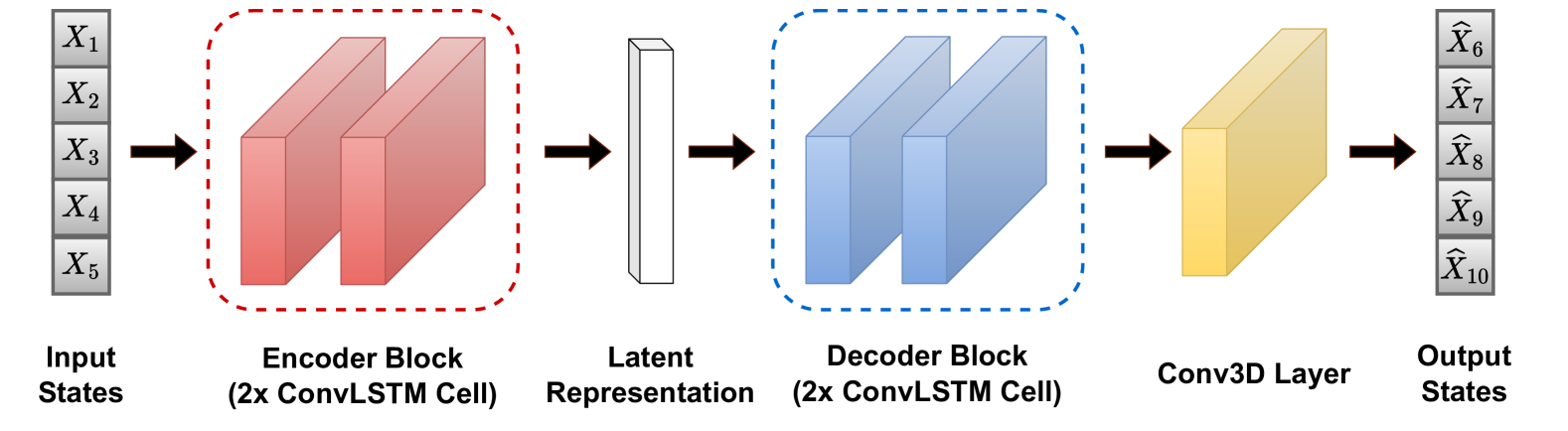
To perform multi-step prediction with ConvLSTMs, a sequence of ConvLSTM cells is structured as an encoder-decoder architecture (also known as Seq2Seq model), where both encoder and decoder blocks contain the same number of ConvLSTM cells. This type of architecture is inspired on sequence-to-sequence (Seq2Seq) models for natural language processing and time-series tasks [Bahdanau (\APACyear2014), Sutskever \BOthers. (\APACyear2014)]. An example is depicted in Figure 1, with two ConvLSTM cells in each block. After an input sequence is processed by the encoder block, the final hidden state from the last ConvLSTM cell forms a compact representation of (latent representation), which is fed to the decoder block to produce the hidden states for each output time step. Finally, a 3D convolutional layer receives the output from the decoder block and produces the predictions of all physical properties for each desired time step. More details about the encoding and decoding processes can be found in [Kakka (\APACyear2022)].
2.3.2 U-Shaped Fourier Neural Operator
Proposed by \citeAwen2022u, the U-Shaped Fourier Neural Operator (U-FNO) is an extension of the Fourier neural operator (FNO) [Z. Li \BOthers. (\APACyear2020)], designed to solve PDEs across diverse problems involving computational fluid dynamics. FNOs are known to be resolution-invariant, meaning that they can be trained on a lower resolution and evaluated on higher resolution, and yield superior performance against conventional CNNs by operating directly on the Fourier space (frequency domain), replacing convolution operations by pointwise multiplications, which are much faster and efficient.
To increase the overall performance in multiphase flow problems, the aforementioned authors introduced the U-Fourier layer as an upgrade of the original FNO architecture, combining the advantages of both CNN- and FNO-based models, increasing both training and test accuracies. On the other hand, this improvement on the accuracies comes in expense of the flexibility of training and testing at different resolutions. Moreover, U-FNO’s usually take a longer time to be trained than traditional FNO’s.
2.3.3 Temporal Attention Unit
Developed for video prediction tasks, Temporal Attention Units (TAUs) [Tan \BOthers. (\APACyear2023)] leverage the ability to capture time evolution in image sequences by introducing parallelizable attention mechanisms that eliminate the need of recurrent-based units (such as RNNs and ConvLSTMs), speeding up the training process. In turn, the spatial modules are represented by simple 2D convolutions. Moreover, not only TAUs account for intra-frame differences through the mean squared error loss, but also for inter-frame variations by embedding a differential divergence regularization term. The resulting loss function is expressed in Equation 3:
| (3) |
where represents the Kullback-Leibler divergence between the probability distributions of the inter-frame differences from and , and is a weight term defined empirically.
3 Methodology
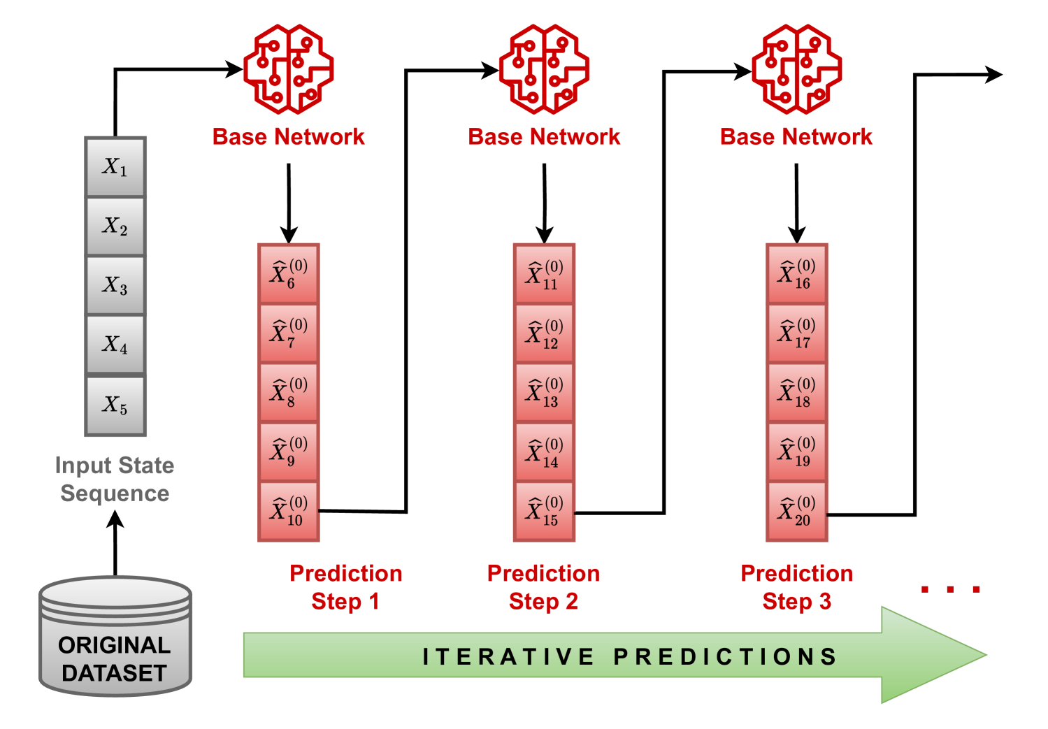
Assuming input steps and output steps, we first train a base network, which is designed to receive a sequence of 5 ”perfect” input states, only predicting the subsequent 5 states (i.e., without successive iterations), as done in a traditional MIMO approach. After the training process, to evaluate the full evolution of the dissolution process on a given simulation containing total steps, we conduct successive iterative predictions, as illustrated in Figure 2, by taking the first 5 input states from , yielding outputs at time steps 6-10. In turn, this output is fed as an input to the same base network to produce the states at time steps 11-15, and so on. Since , the total number of iterative steps is .
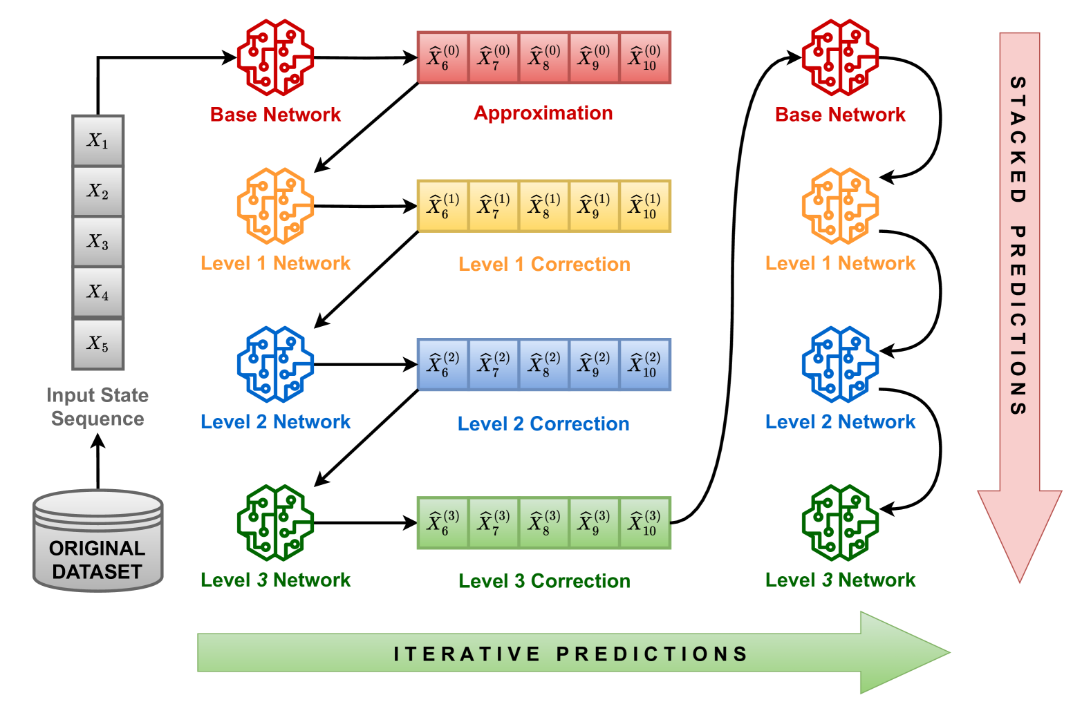
To improve the initial solution produced by the base network, we propose a multi-level stacking of trained networks. In this case, the same neural network architecture is used to train each level, with the same sizes for both input and output tensors as the base network, as well as the loss function. Considering the base network as Level 0, trained with a dataset , where is the number of training samples, we generate a new dataset comprised of all possible output sequences computed by the base network for each , representing initial approximations to the true states . The Level 1 network is then trained to receive, as input, one of those responses produced by the base network, and outputs a new approximation (correction) to the ground truth within the same time-step interval, hypothesizing that it will yield less errors than the initial solution. Following this rationale, we can continue the stacking process by training a Level 2 network with the outputs produced by Level 1, and so on until no further improvement is observed. During this process, only one level can be trained at a time.
In general, let be the number of levels of correction to be applied on the base solution. After the base and all of the correction networks are trained, the iterative multi-step prediction process can be conducted as illustrated in Figure 3 with . Here, the first 5 input states of a simulation sample are fed into the base network, producing an initial approximation for the subsequent 5 states. Then, this output is fed to the Level 1 network which produces the first level of correction for the initial approximation. Later, this output serves as input to Level 2 network, whose output is forwarded as an input to Level 3 network, which yields the final prediction for time steps 6-10. For the next prediction step, the output from the last network of the stack is fed to the base network to produce an initial approximation for steps 11-15, which is corrected by the subsequent levels in the stack. The whole process is repeated until the simulation end time.
4 Reactive Dissolution Dataset and Preprocessing
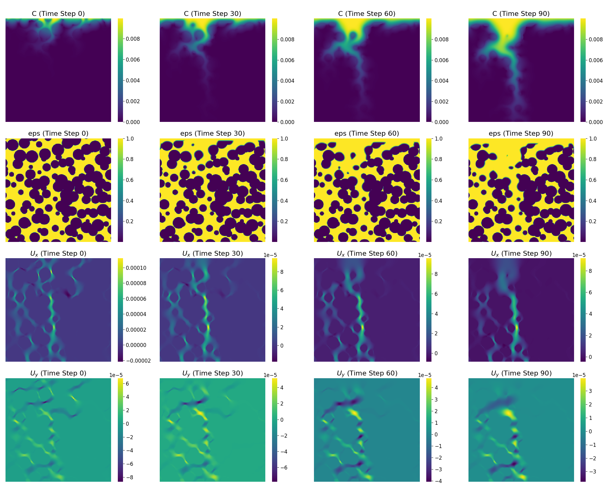
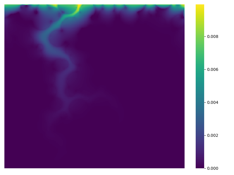
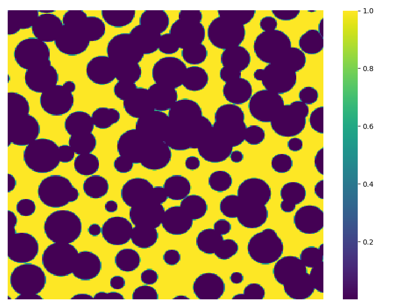
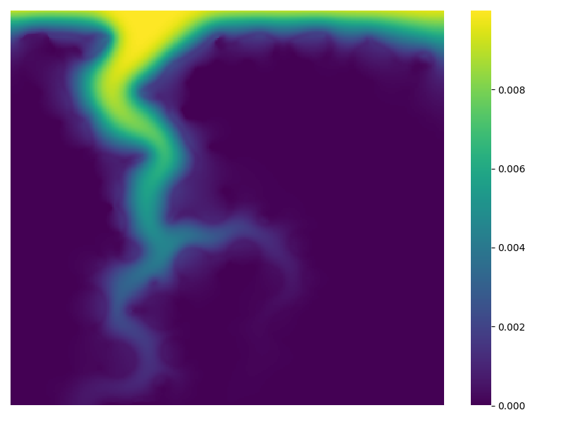
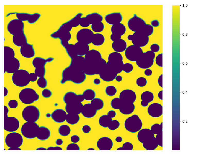
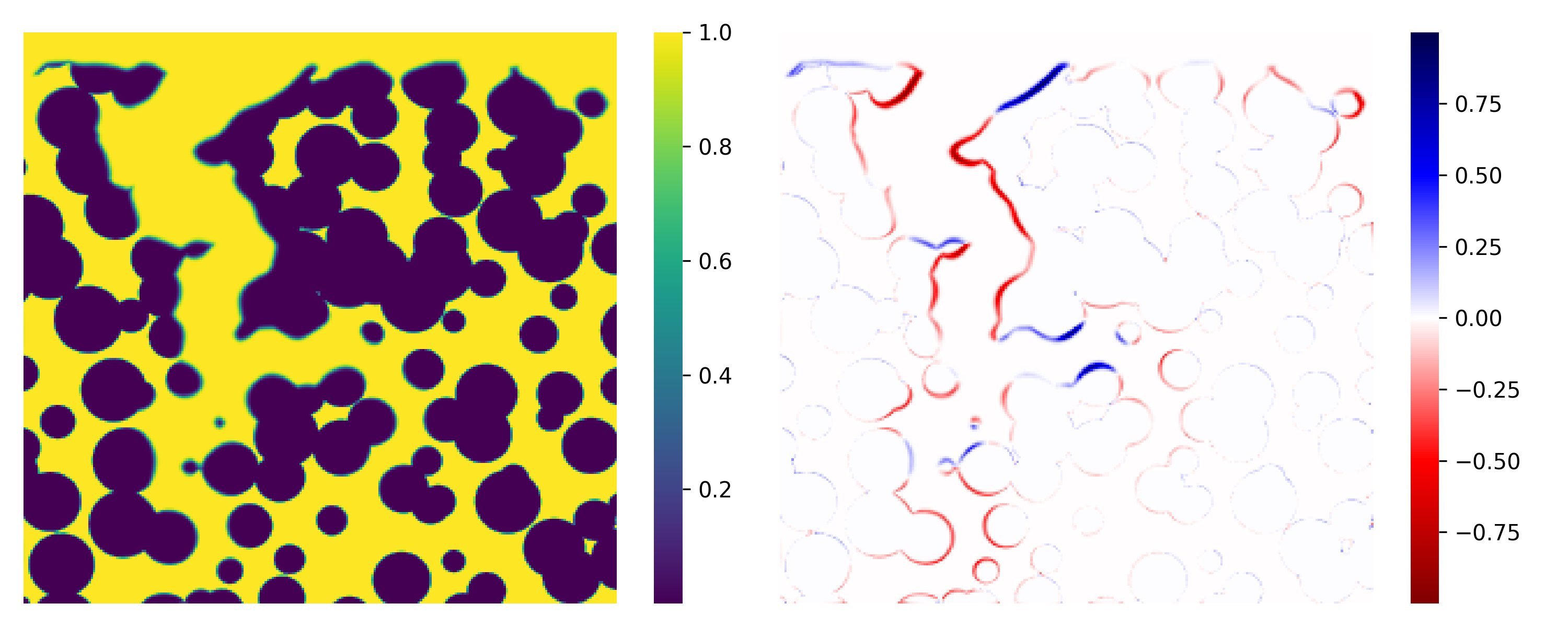
Our reactive dissolution dataset 111https://doi.org/10.5281/zenodo.14974427 is comprised of 32 numerical simulations produced by GeoChemFoam [Maes \BOthers. (\APACyear2022)]222https://github.com/GeoChemFoam, an open-source tool that models pore-scale reactive dissolution in porous systems. The 2D simulation results are stored at 100 equally spaced time steps, resulting in time-evolving dissolution state maps of size . For the ML algorithms tested in this work, all maps were cropped to by removing the first and last two rows and columns from each state map. Each of these simulations conveys a particular rock sample with its own pore structure, as well as a distinct fluid trajectory over the course of the dissolution process. An example is illustrated in Figure 4. These maps encompass four different input properties: , the concentration of the acidic solution used in the dissolution; , a function indicating the volume fraction of the pore space occupied by pore in each voxel, which is proportional to the amount of fluid contained in each voxel; , the magnitude and direction of flow of the acidic solution in the horizontal axis of a 2-D Cartesian plane; and similarly , for the vertical axis. The average time to produce each simulation was approximately 3 hours using 24 CPUs of 3 GHz each. All simulations employ the same flow and reactive transport conditions, where both Péclet and kinetic numbers are equal to 1.
In essence, GeoChemFoam solves the reactive transport in porous media in a quasi-static regime, as described by Maes et al. \citeAmaes2022improved. Given a porosity map at a time step , it first calculates the steady-state velocity (i.e., it produces and at time step ). Then, it calculates a steady-state concentration at time step , which includes the contributions of injection, diffusion, and reactive dissolution at the fluid-solid interface. From these calculations, it estimates a local reaction rate in each computational fluid and the new field for the time step , which in turn is used to calculate the flow once again to produce a new map at time step , and so on.
Aside from the original features, three extra input features were engineered as an attempt to improve the performance of all DL models: 1) Magnitude of velocity: defined as ; 2) Scaled, a log-transformation over the concentration values; and 3) Combined Filter, a binary mask based on and constraints which shows the portions of the grains in a porous matrix that are being dissolved at a particular time step . Given a position in a map, the combined filter is calculated according to Equation 4:
| (4) |
5 Performance Evaluation of Deep Learning Models
In this section, we will discuss the quantitative and qualitative results of our proposed method on all algorithms described in Section 2.3. The source code is available at https://github.com/ai4netzero/ReactiveDissolution.
5.1 Training and Evaluation Settings
From the 32 simulation samples in our dataset, 24 were randomly selected as the training set and the remaining 8 as the validation/test set. Before the DL models are trained, the entire data is normalized with respect to the mean and standard deviation values of the training set. All input features, except for C Scaled and the Combined Filter, have their original values subtracted by their respective means and the results are each divided by their respective standard deviations. On the other hand, a min-max normalization is applied to the output values so that they all belong within the range, making it suitable to adopt the sigmoid activation function for all DL models.
Concerning our proposed multi-level stacking of neural networks method, for each DL algorithm described in Section 2.3, we perform corrections up to Level . The models were trained on a NVIDIA Titan RTX with 24 GB of memory for a total of 100 epochs (along with a patience rate of 20 epochs for early stopping), using a batch size of 4, a learning rate of 0.0005 and the Adam optimizer [Kingma (\APACyear2014)] with moment values and . The mean squared error was adopted as the loss function for ConvLSTM, U-FNO and the intra-frame difference term of TAU. Regarding the latter, the constant for the regularization term (inter-frame difference) was fixed at 0.1.
For the quantitative evaluation of the iterative predictions of each output property, we calculate the Pearson correlation coefficient (PCC) to assess the similarity between the predicted state and the ground truth state at each time step, as stated in Equation 5:
| (5) |
where cov is the covariance between and and represents the standard deviation of a state map.
5.2 Model Statistics
Table 1 shows some statistics about the average training epoch times, numbers of trainable parameters, final model sizes and average forward times (i.e., the elapsed time for processing input data through a network to produce the next 5 time steps) for each DL model. Although TAU has the highest numbers of trainable parameters and a relatively larger model size, it still achieved the lowest training and forward times, due to its recurrence-free structure.
| DL Model |
|
|
|
|
|
|||||||||||
| ConvLSTM | 6.44 | 10.73 | 4 M | 13 | 60 | |||||||||||
| U-FNO | 10.98 | 18.30 | 6 M | 25 | 79 | |||||||||||
| TAU | 4.22 | 7.03 | 11 M | 135 | 33 |
Despite being the most lightweight model, ConvLSTM has a 50% slower training time per epoch than TAU, also taking nearly twice as long for the forward operation. Finally, U-FNO achieved the slowest training and forward times, but the resulting model after the training process is about five times smaller than TAU and almost two times bigger compared to ConvLSTM.
Analyzing the total runtime of each algorithm to produce a 100-step simulation, TAU takes an average time of 0.66 seconds, followed by ConvLSTM (1.2 seconds) and U-FNO (1.58 seconds). These represent a speedup with an order of magnitude between and when compared to the average time taken by GeoChemFoam (3 hours).
5.3 Iterative Prediction and Model Stacking Analysis
Figure 5 shows the average correlations of the iterative predictions on all training samples for all algorithms and correction levels. For all properties, it can be observed that both TAU and U-FNO are more robust to error accumulation, with the latter achieving slightly higher correlations at late time steps. With respect to each output property, the best results were achieved for prediction, followed by the concentration , and the flow directions and .
Considering the effects of model stacking, ConvLSTM achieved its best results at Level 2 correction (except for prediction). Still, it was not capable of performing better than the base networks (Level 0) of the other two algorithms. TAU showed no significant improvement when applying multi-level stacking for all cases, as evidenced by the fact that the correlations do not systematically increase over the correction levels. On the other hand, U-FNO showed a more consistent evolution from the base network to Level 3 in all scenarios, as the average correlations at the late time steps typically increase after each correction.
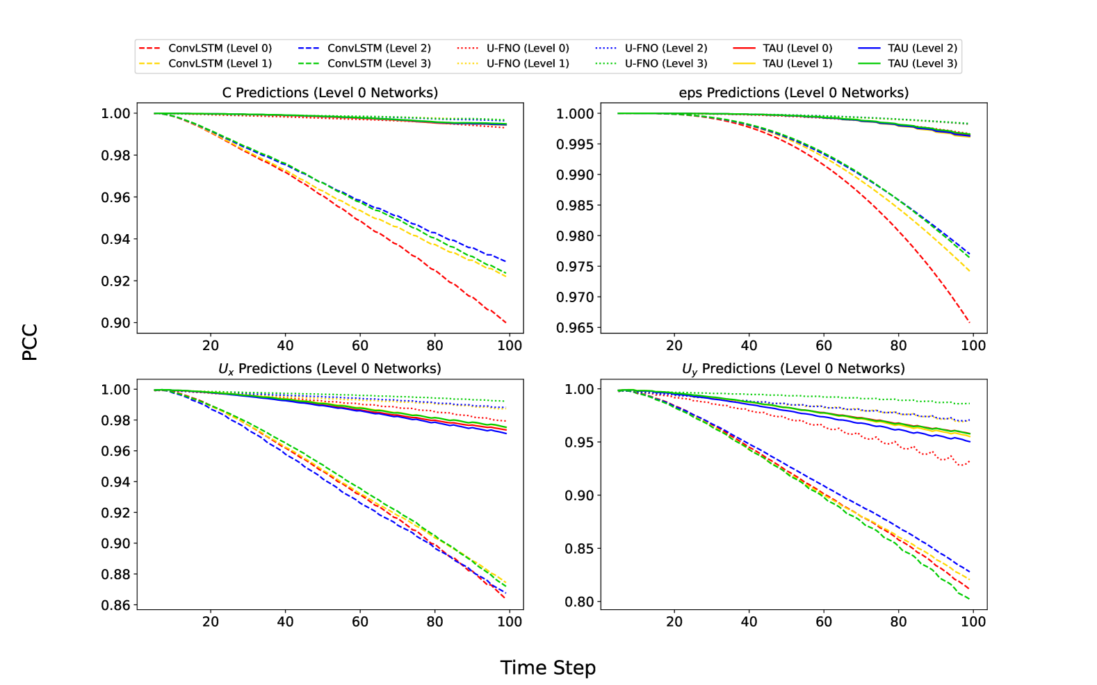
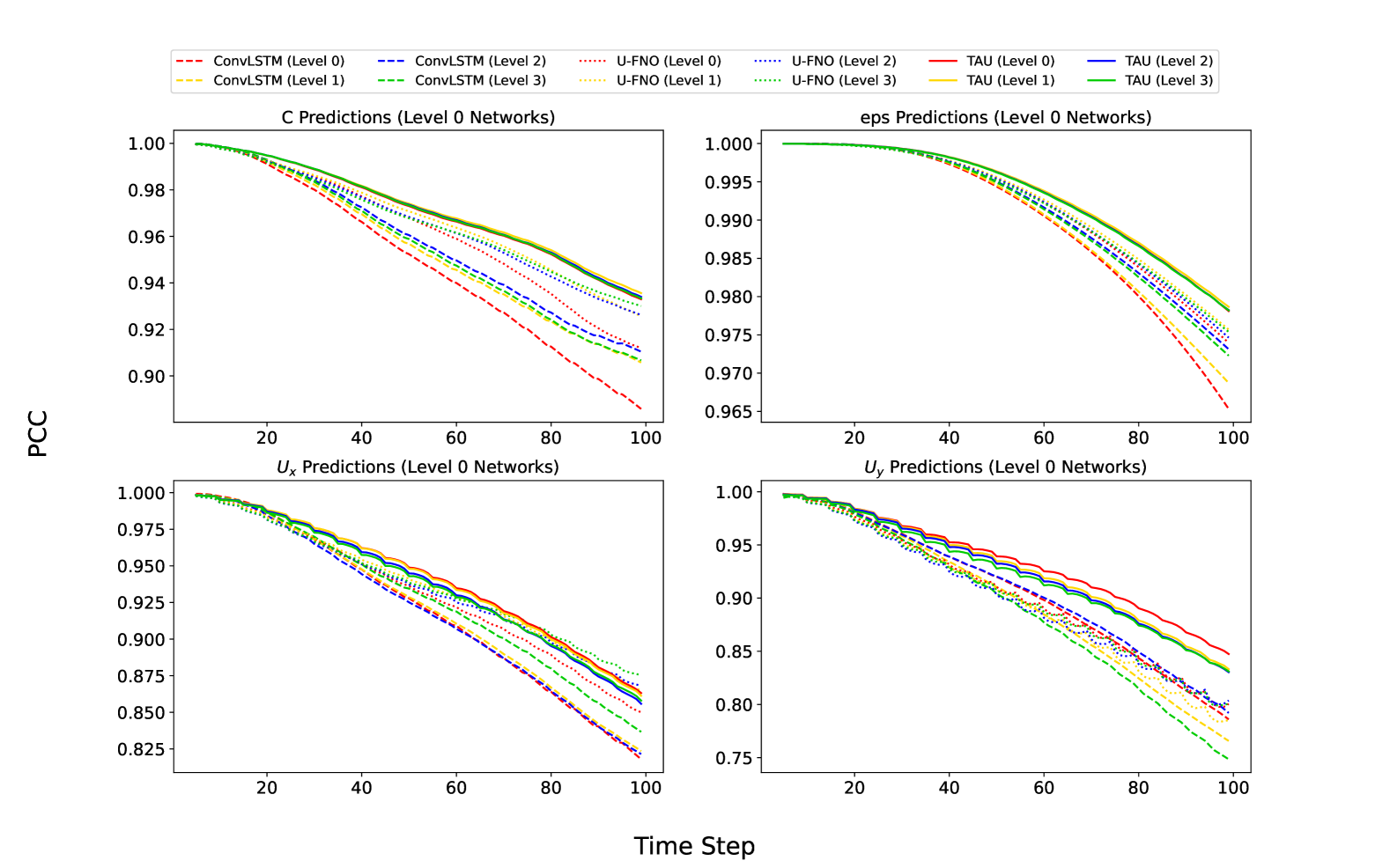
Figure 6 illustrates the results for the validation set. The plots show that TAU achieved the best iterative predictions for all cases (except for prediction). Apart from ConvLSTM, the correlations had a reasonable drop when compared to those from the training data. However, this drop is much larger for the U-FNO, suggesting that this network is much more prone to over-fitting than the others.
Regarding the performance evolution along the correction levels, ConvLSTM still yielded its best results on Level 2 network, except for prediction, in which Level 3 was more robust to error accumulation. However, it achieved the lowest correlations in almost all scenarios, being only superior to U-FNO in the prediction of . The validation curves for U-FNO, unlike the results for the training set, did not show a consistent evolution over the levels. For instance, in the prediction of , the Level 1 network achieved the best results until time step 80, where it was surpassed by Level 3. Moreover, Level 1 prevailed as the best correction network during all time steps of prediction. Finally, the Level 1 network from TAU achieved the highest correlations for predictions of and , as well as for predictions until time step 50. Despite its better performance against ConvLSTM and U-FNO, the multi-level stacking strategy did not cause a significant improvement over the TAU Level 0 network.
To ratify the robustness of our method by evaluating it with a different metric, we refer to A.
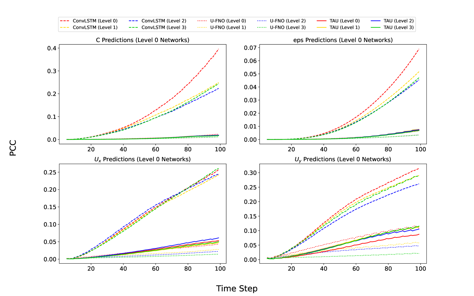
5.4 Relevance of Engineered Features
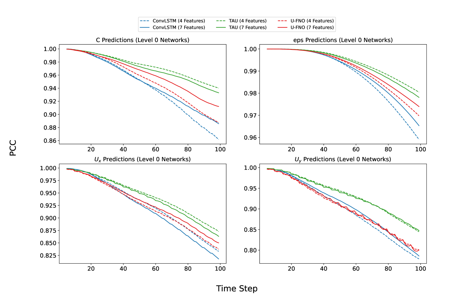
Figure 7 illustrates the effects of including the three engineered features described in Section 4 along with the four original input properties. To provide a clear visualization of these effects, we will only discuss the results with respect to Level 0 networks. From the plots, we can notice that for both ConvLSTM and U-FNO, there is a performance drop when transitioning from 7 to 4 input features, except for predictions for ConvLSTM. Moreover, U-FNO with 4 input features achieved better results than ConvLSTM with 7 input features.
Conversely, TAU yielded slightly better performances without the engineered features, also achieving superior results than the other two methods. However, a further analysis with respect to its internal parameters (including the term of the loss function) must be conducted to confirm whether the engineered features are actually relevant. Nevertheless, the plots demonstrate TAU’s capability to understand the evolution of the reactive dissolution process with a smaller set of input features.
5.5 Qualitative Analysis
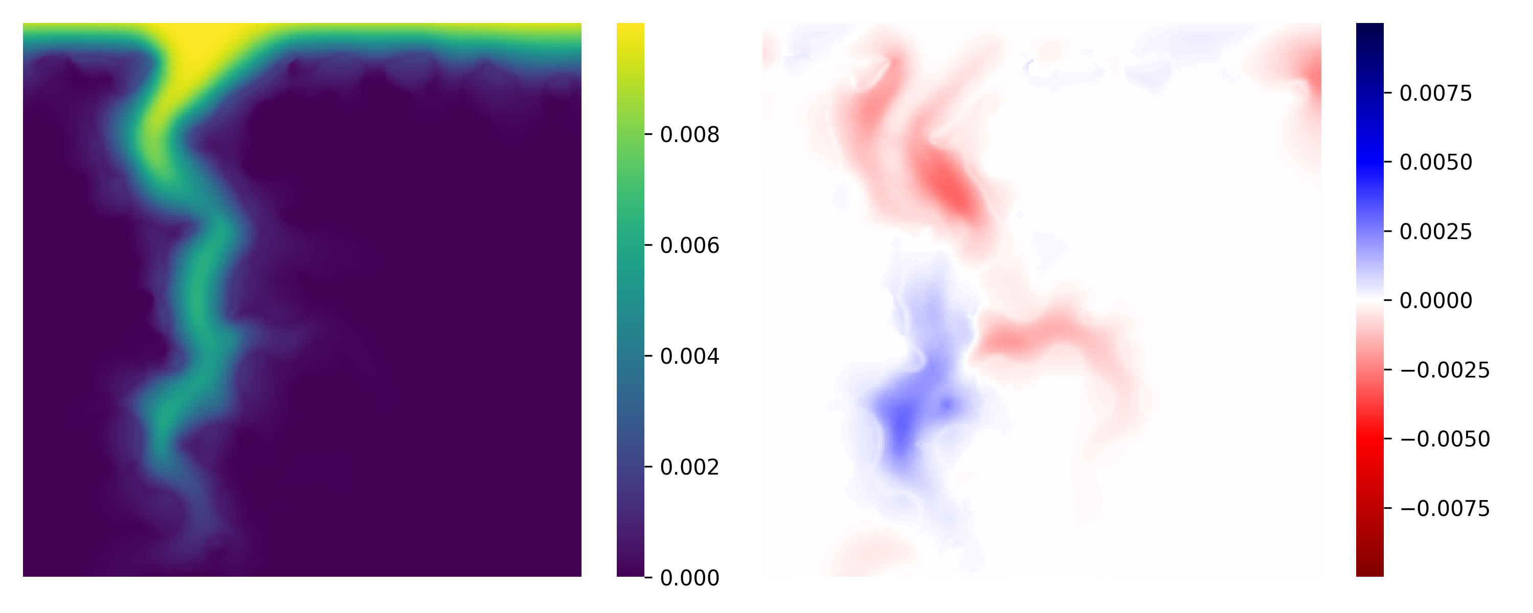
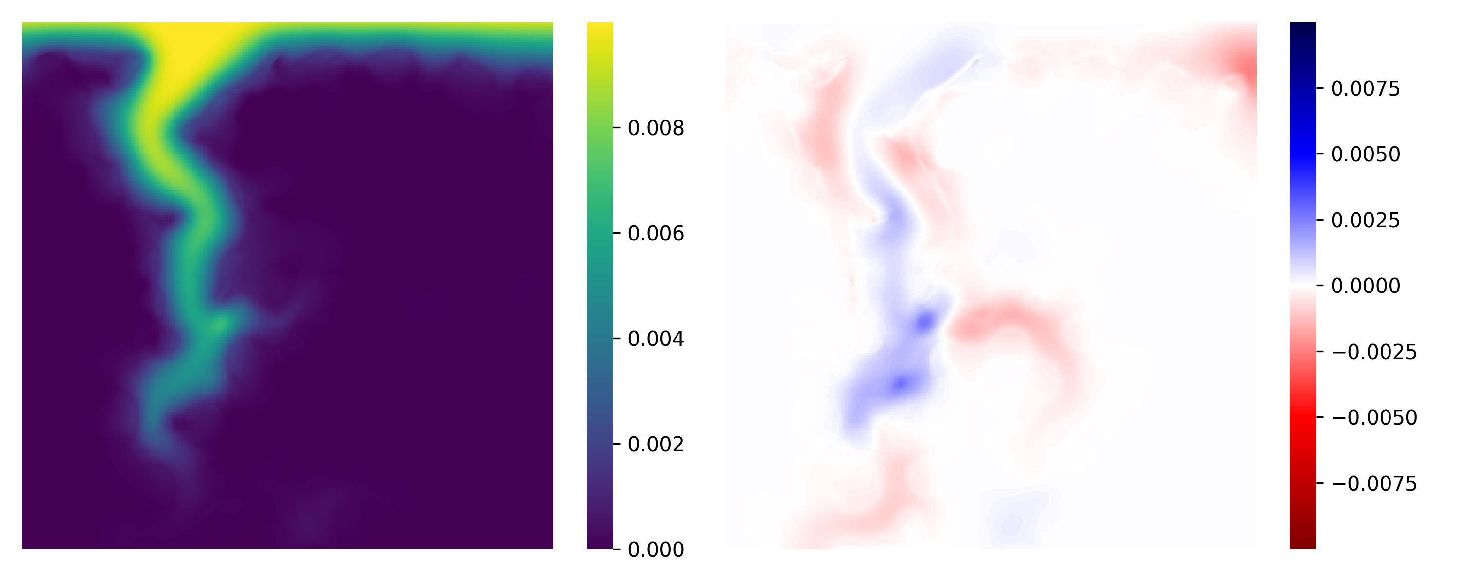
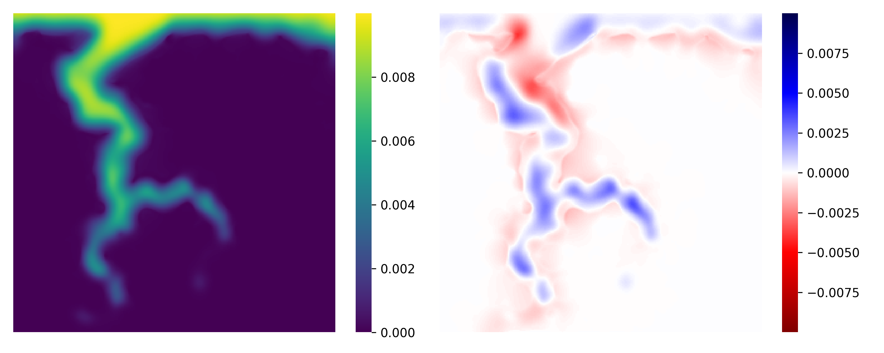
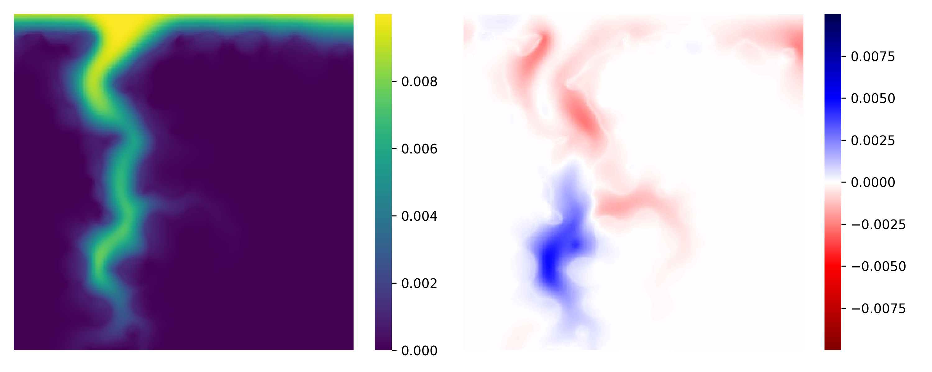
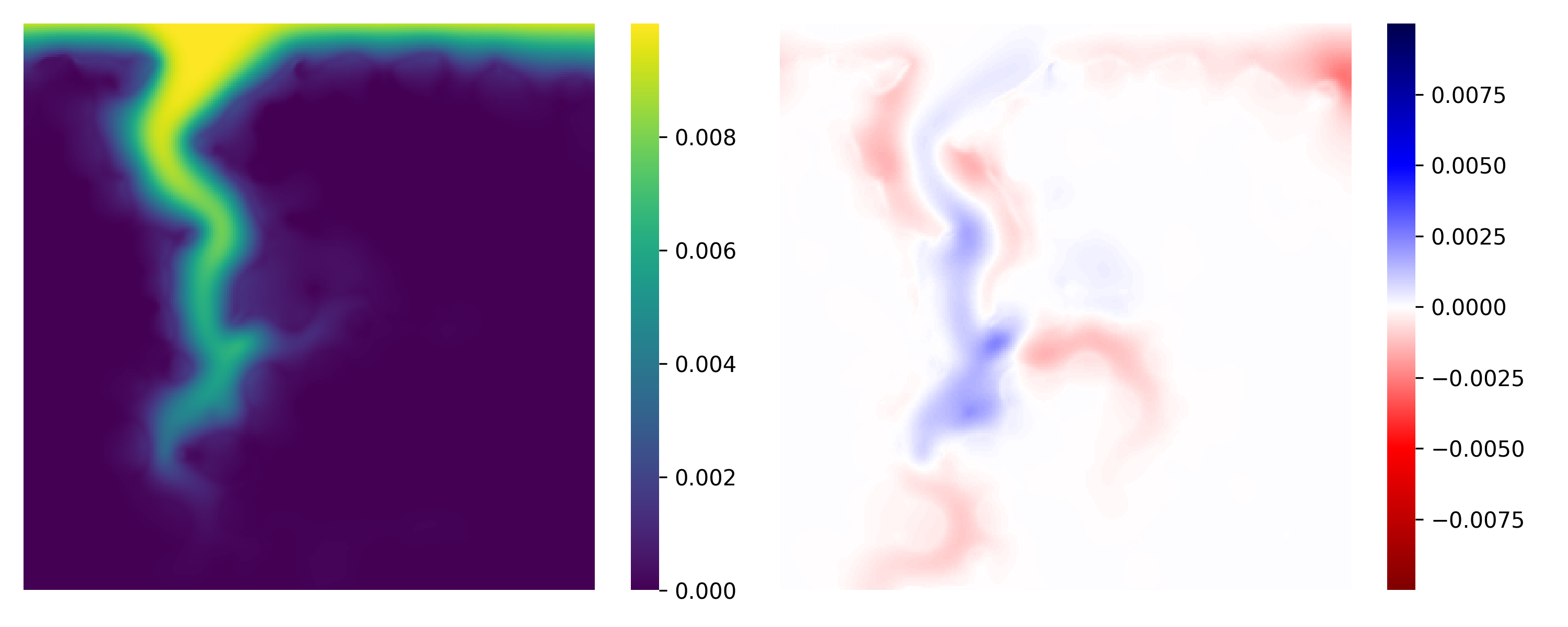
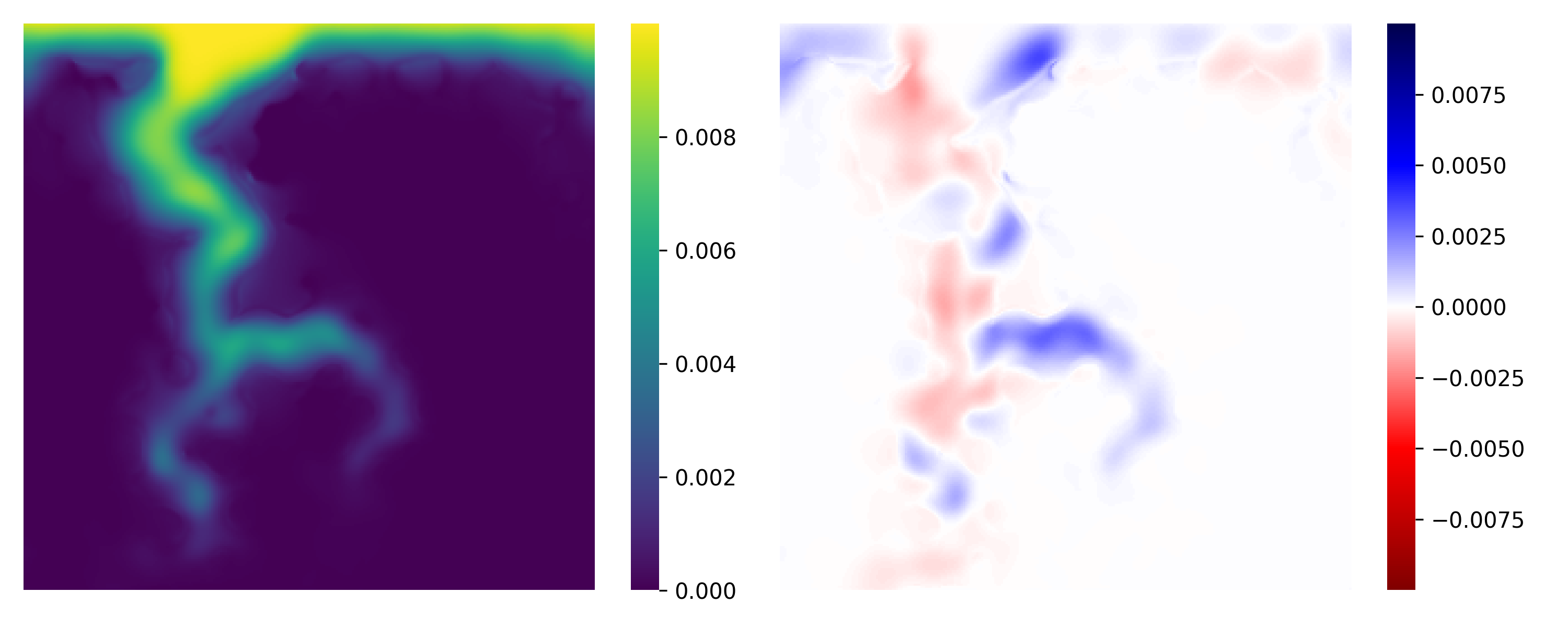
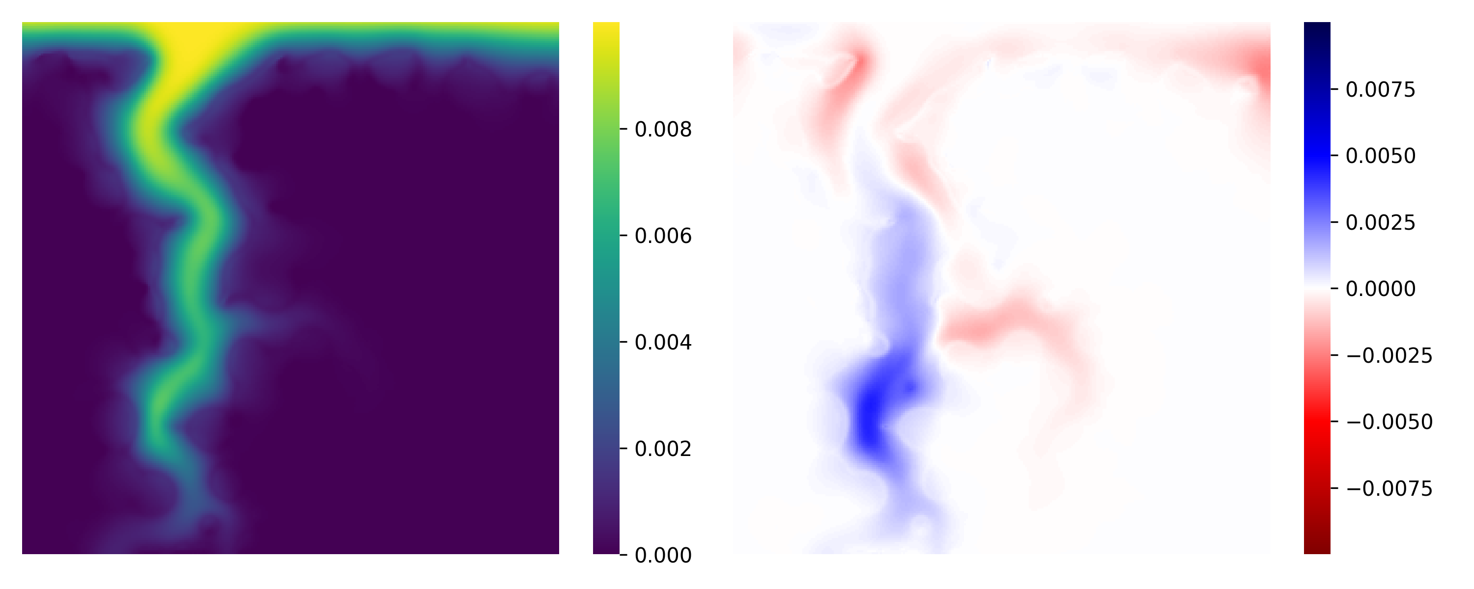
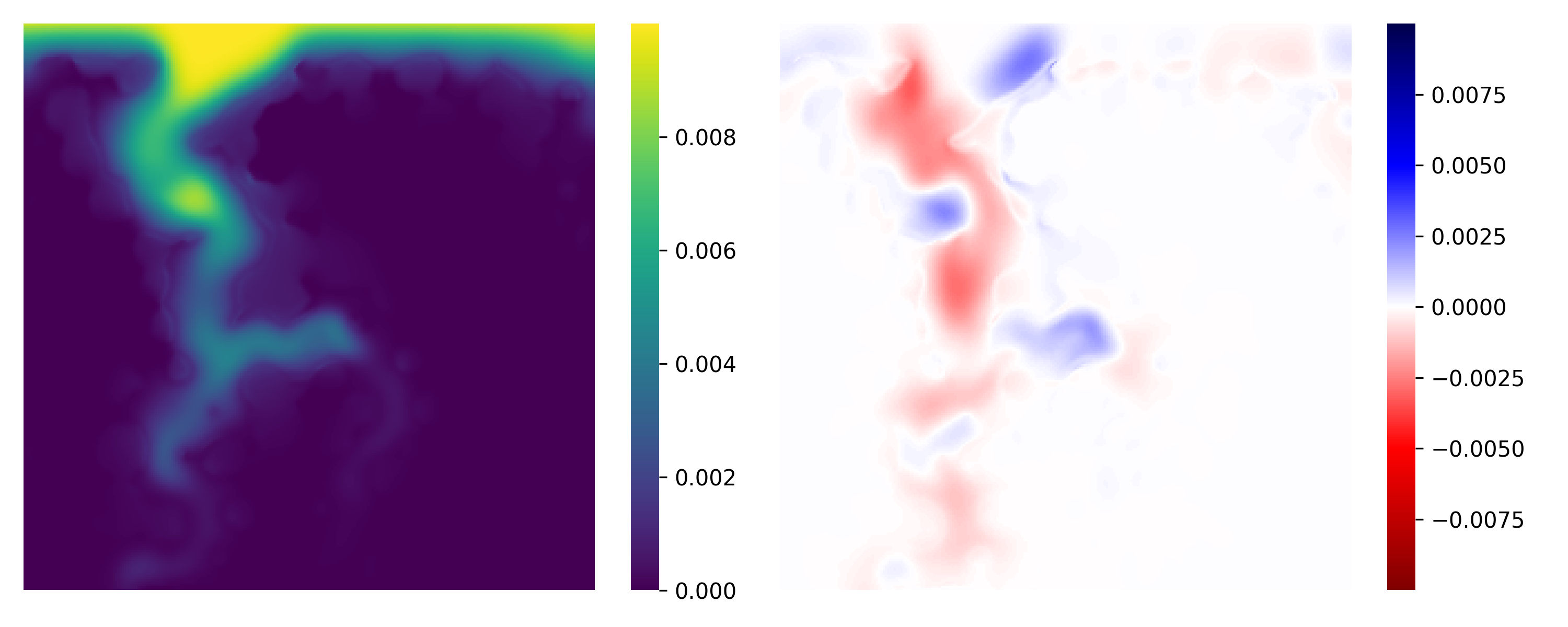
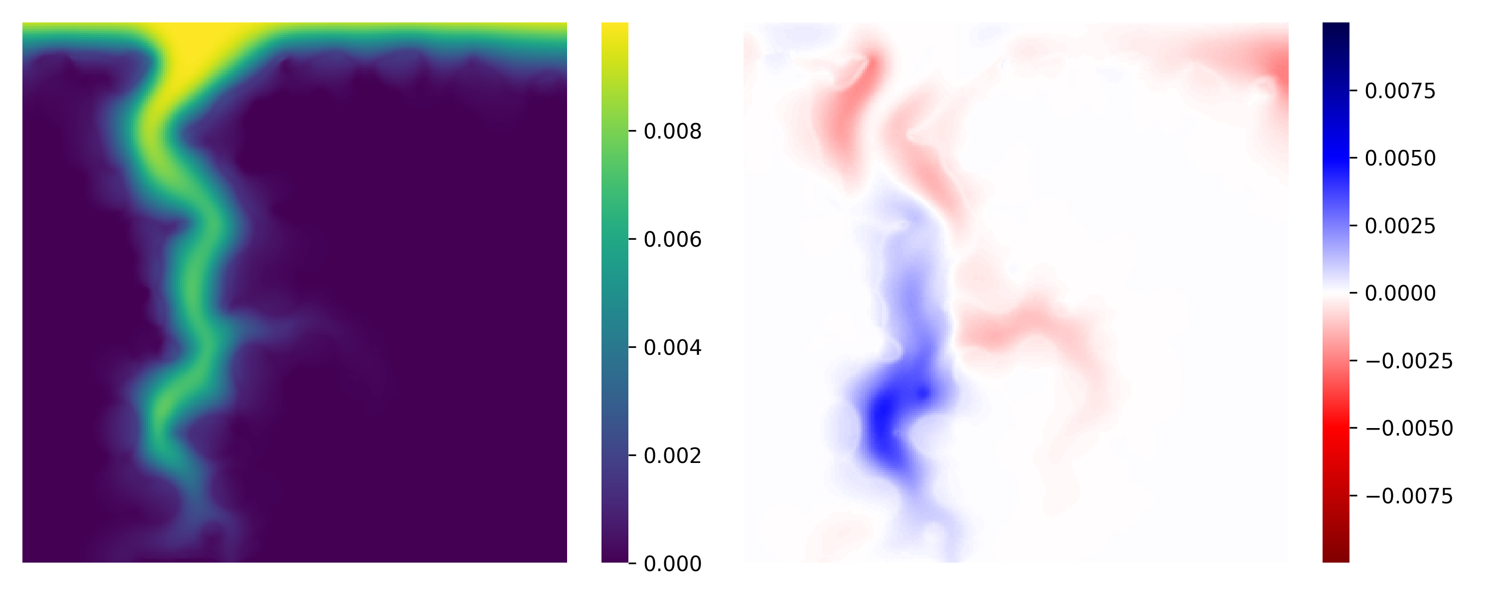
In this section, we will conduct a qualitative analysis on a sample from the validation set, comprising a particular pore geometry. Herein, we will consider the predictions at the last time step (100) after several iterative steps are performed for each algorithm. To simplify our analysis, we only show the predictions for and fields. Figure 8 shows the ground truth maps for those two properties at time steps 0 and 100.
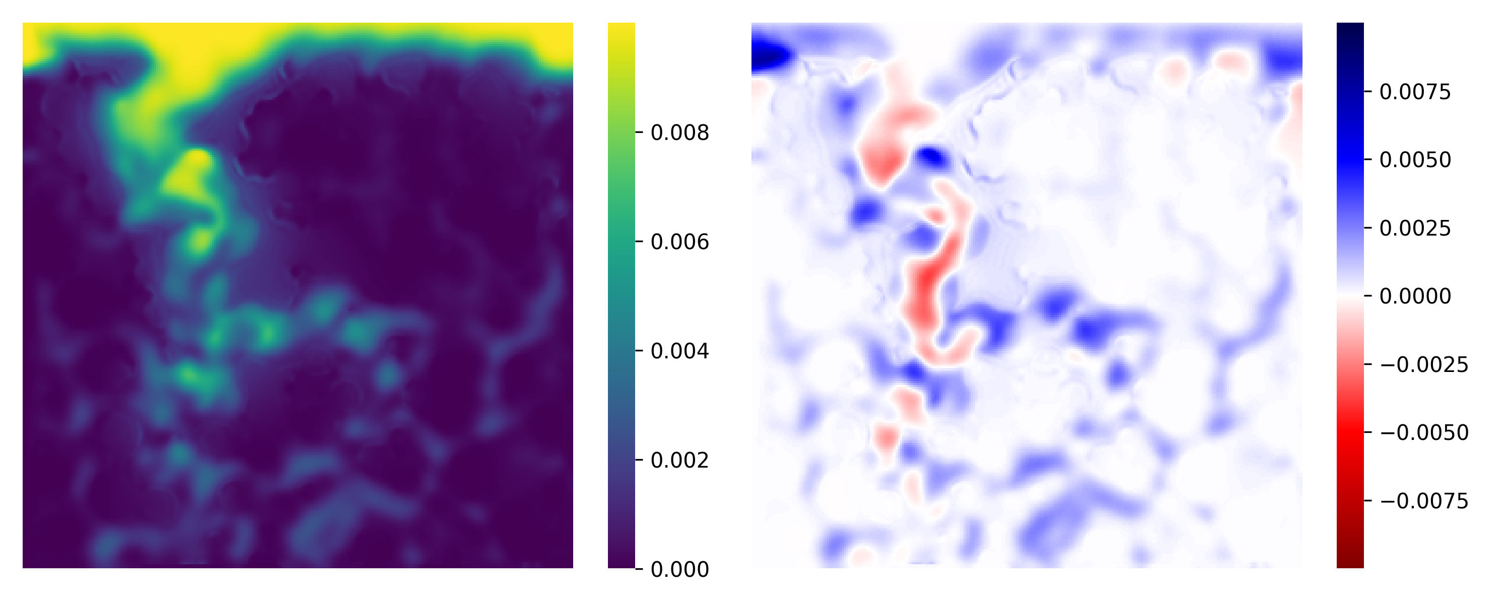
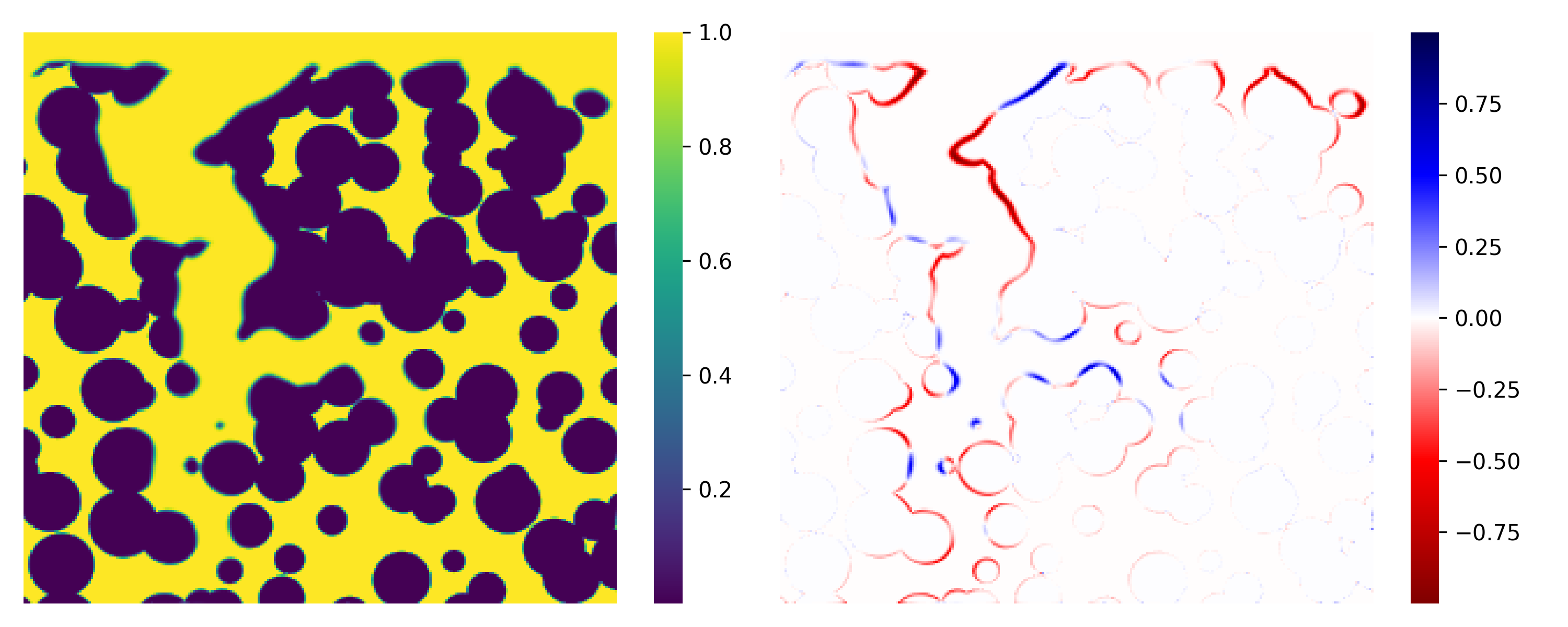
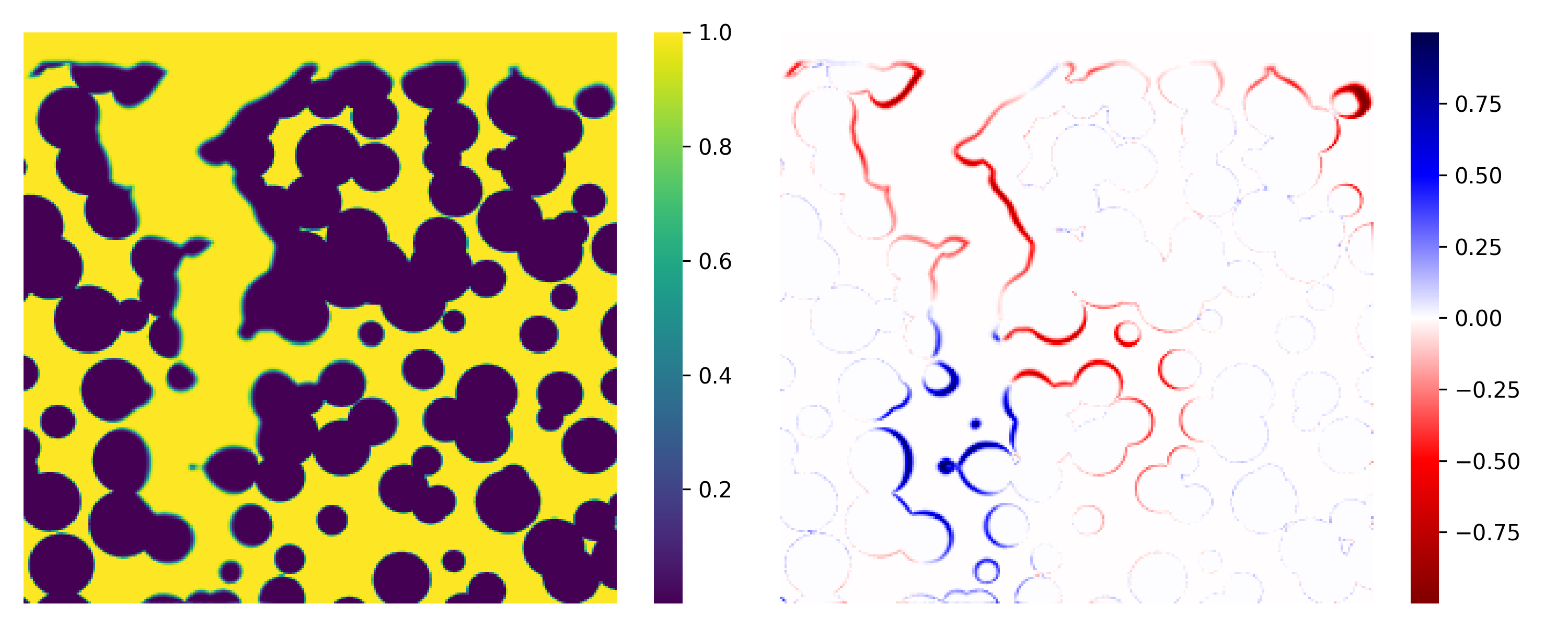
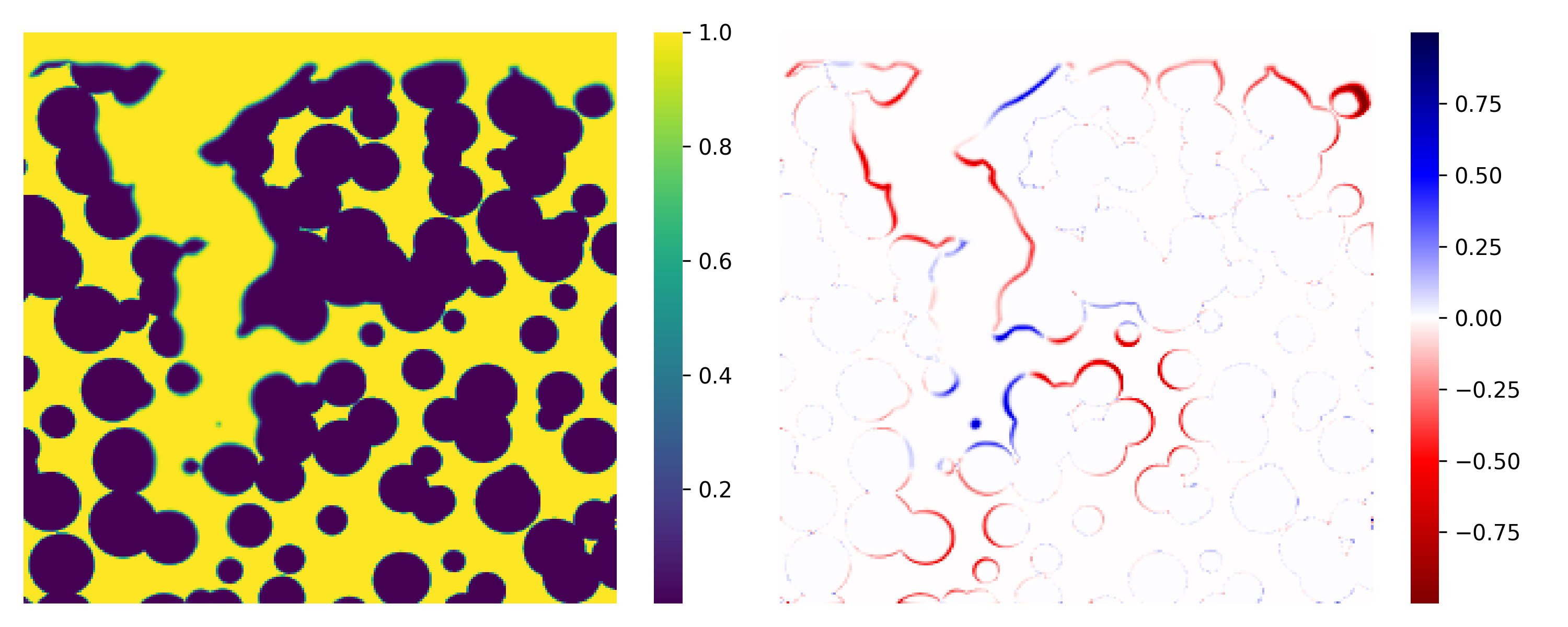
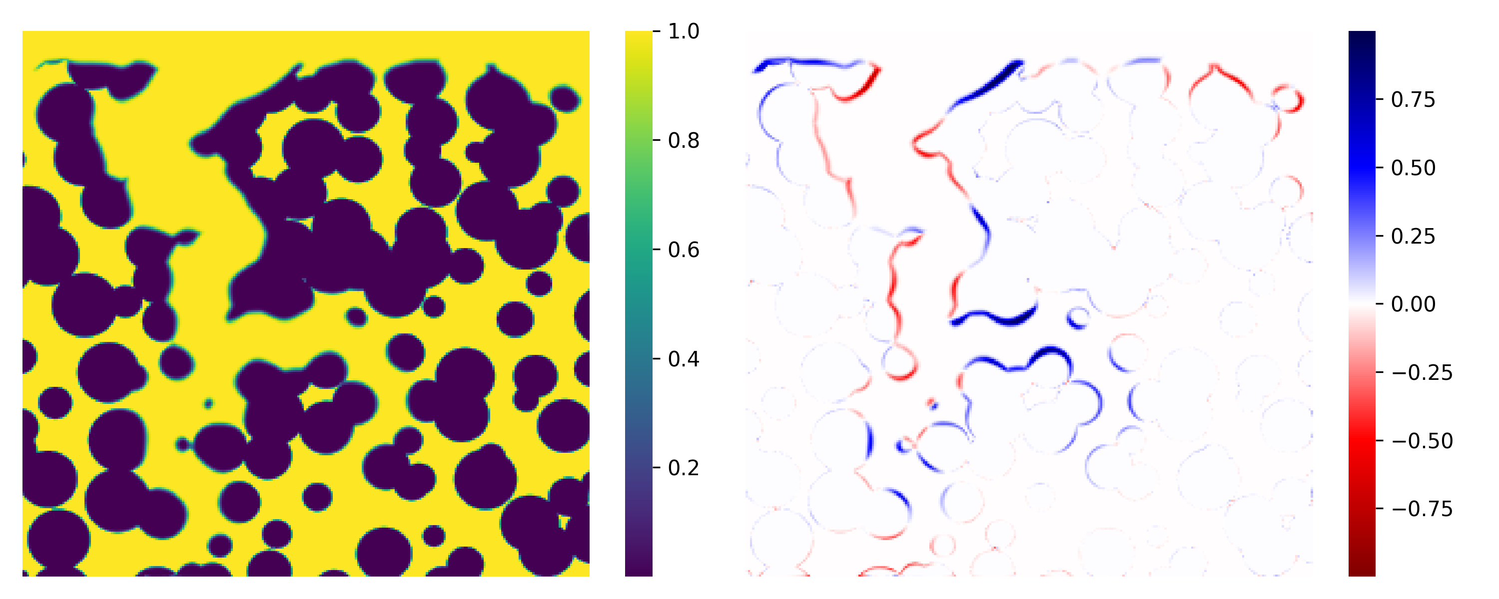
The predictions of for all algorithms and all network levels are displayed in Figure 9, along with their respective difference maps to the ground truth (). We can notice a clear evolution on the ConvLSTM results, as the results are Level 0 contain too much noise, which is mostly mitigated over the subsequent levels. However, there is a slight decrease in the PCC score from Level 2 to Level 3. Regarding U-FNO, the best results were achieved at Level 0, which yielded a PCC of 0.004 lower than ConvLSTM Level 2. Moreover, all levels produced similar shapes of dissolution channel, only missing the right branching at the bottom-center part of the map. Finally, although not having benefitted from the multi-level stacking approach, TAU achieved the highest scores for all levels, where even its Level 0 network performed better than any other level from both ConvLSTM and U-FNO. Looking at the difference maps, we can also notice a smaller range of errors compared to the other two algorithms. With respect to the dissolution shape, it was able to capture some of the right branching, but not as much as ConvLSTM did.
PCC = 0.944
PCC = 0.975
PCC = 0.987
PCC = 0.969
PCC = 0.956
PCC = 0.987
PCC = 0.979
PCC = 0.965

PCC = 0.987
PCC = 0.976
PCC = 0.961

PCC = 0.986
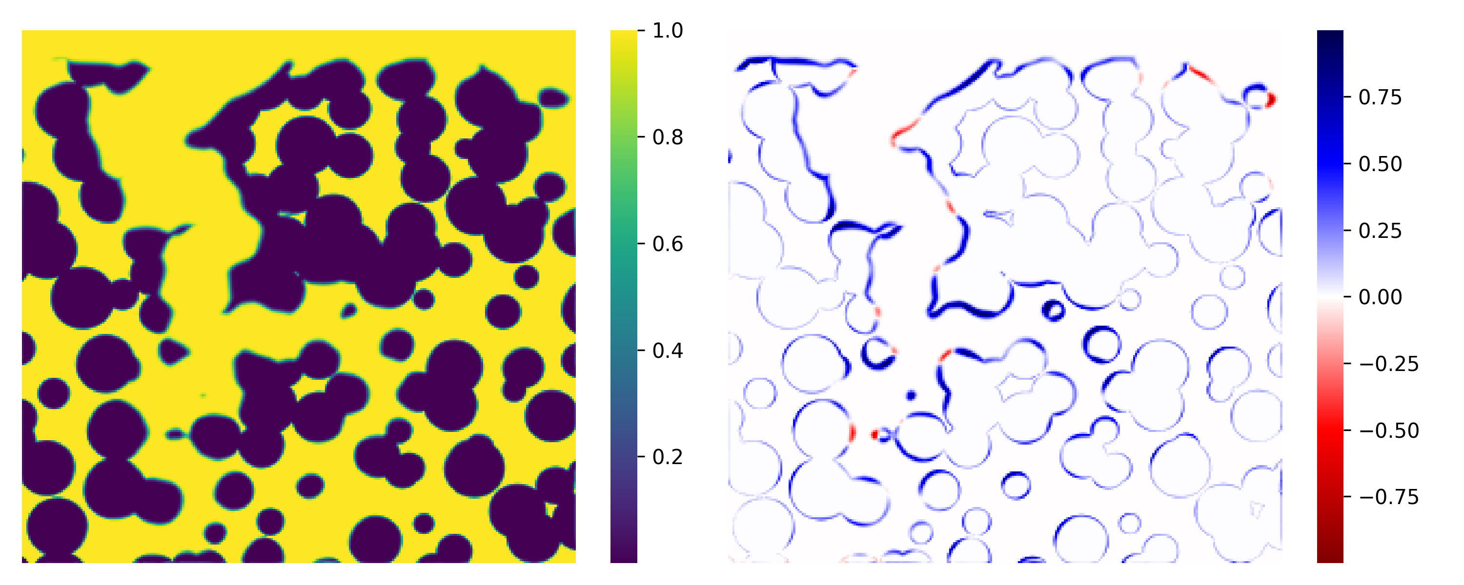
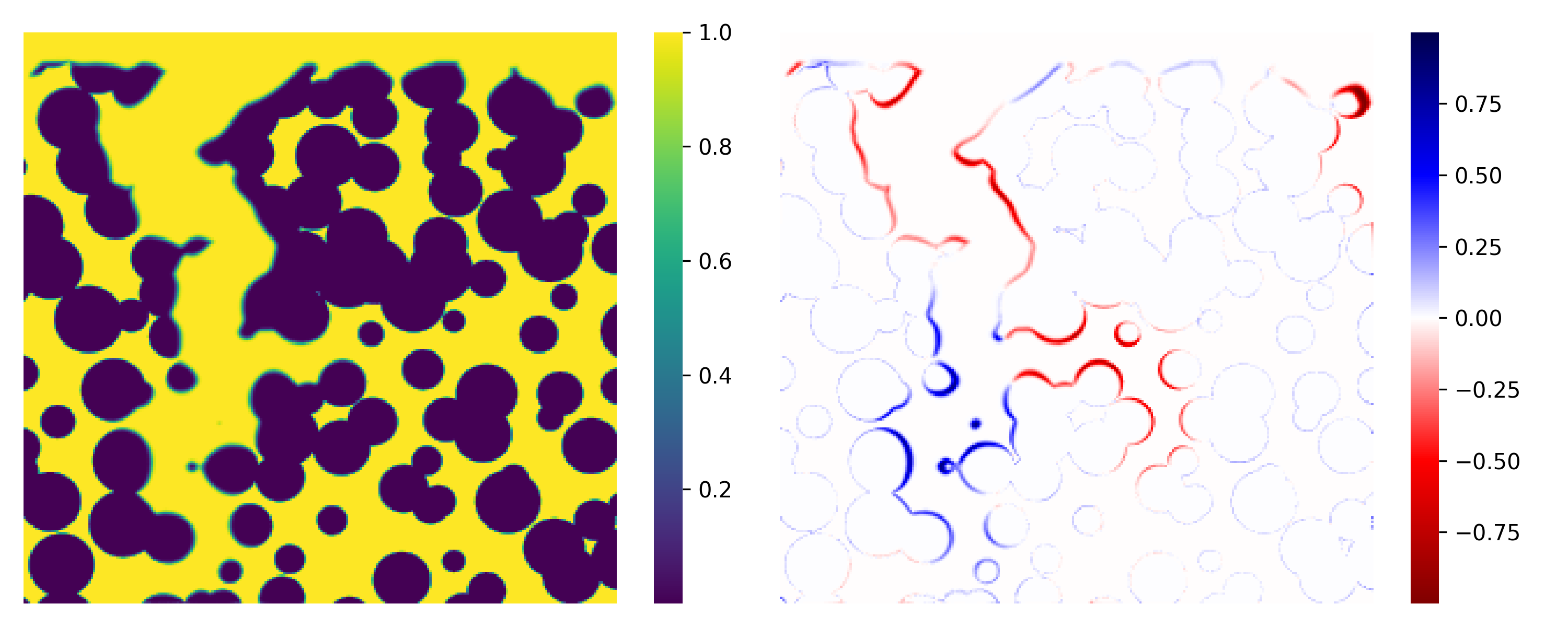
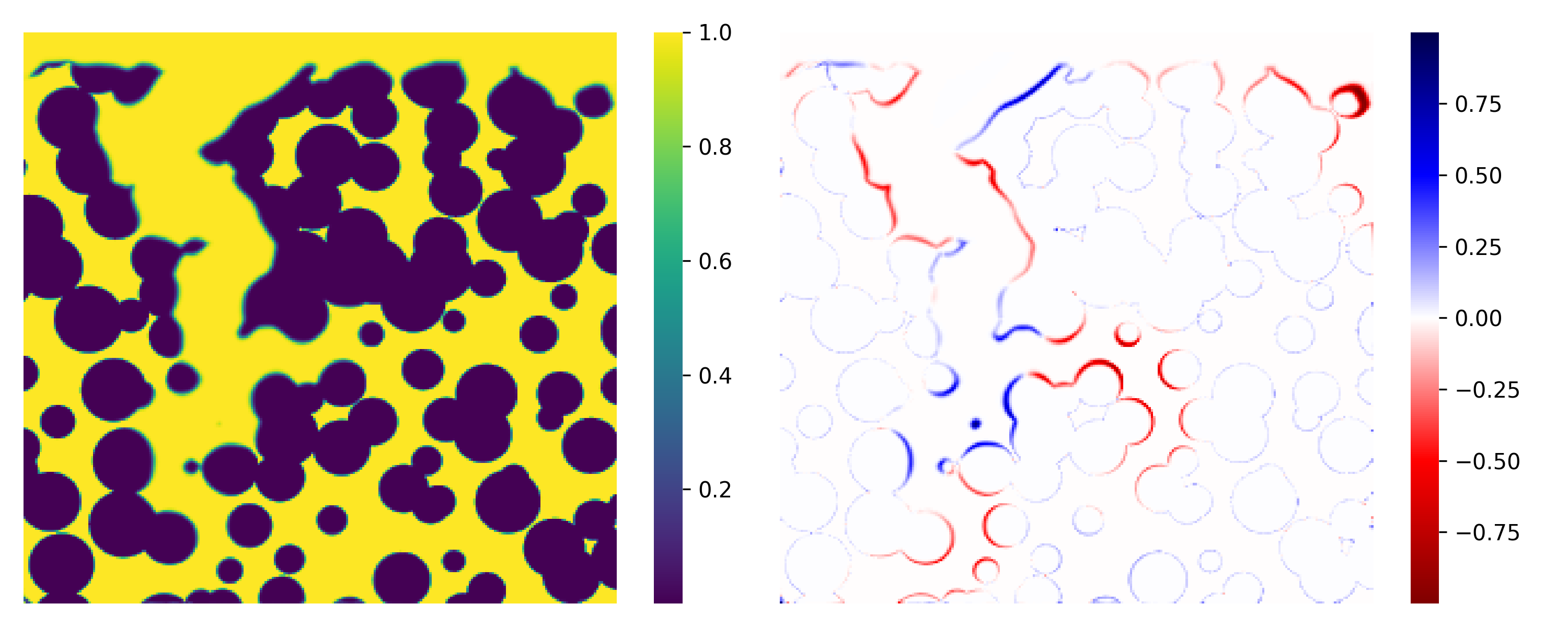
Figure 10 shows the predictions for at time step 100. In general, all networks managed to yield nearly perfect predictions when compared to the ground truth. The PCC scores for ConvLSTM strictly increase over all levels. At Level 0, we can notice a prevalence of overpredictions all over the map, which is mitigated at the subsequent levels. On the other hand, neither U-FNO nor TAU showed significant differences from one level to another, with the latter achieving the best PCC scores at each level, having only tied with ConvLSTM at Level 3.
PCC = 0.979
PCC = 0.989
PCC = 0.992
PCC = 0.990
PCC = 0.985
PCC = 0.991
PCC = 0.991

PCC = 0.988

PCC = 0.992
PCC = 0.992

PCC = 0.987

PCC = 0.992
5.6 Estimation of Bulk Properties
To convey a better understanding of the overall dissolution dynamics in our case study, we analyze the evolution of two of the bulk properties used for modelling reactive dissolution at the field-scale: porosity and permeability. For each sample from our validation set, we selected 10 maps, starting at time step 5, with an offset of 10 time steps between each pair of consecutive maps, ending at time step 95. We repeated this process for the maps predicted by each of the DL algorithms at the aforementioned time steps. The porosity and permeability values for all maps are then calculated using GeoChemFoam, and the results achieved by each algorithm are compared against the ones obtained from the original data.
For all cases discussed in this section, we will show how the errors of porosity and permeability for each algorithm evolve due to the dissolution process in terms of: 1) their respective average values; and 2) the RMSE error versus the values from the ground truth (referred as ”Original Data” in the subsequent plots).
5.6.1 Porosity Estimation
Figure 11 shows the average error in porosity considering all models from the training set. Looking at the average evolution over the sampled time steps (Figure 11), we observe that the curves from U-FNO and TAU are the closest from the original porosity values, especially at late time steps, where the error tends to be higher due to the error accumulation problem of the iterative approach. Conversely, the curves from ConvLSTM are farther away from the ground truth, even though it shows some improvement over the network levels. In the RMSE curves (Figure 11), we observe that TAU Level 3 achieved the lowest errors on time steps 25 and 35, but ends up with a higher error than its Level 0 counterpart and all U-FNO variants (except U-FNO Level 0). Both ConvLSTM and U-FNO showed a more consistent evolution over the network levels, whereas the U-FNO Level 3 having lowest errors at the end of the dissolution.
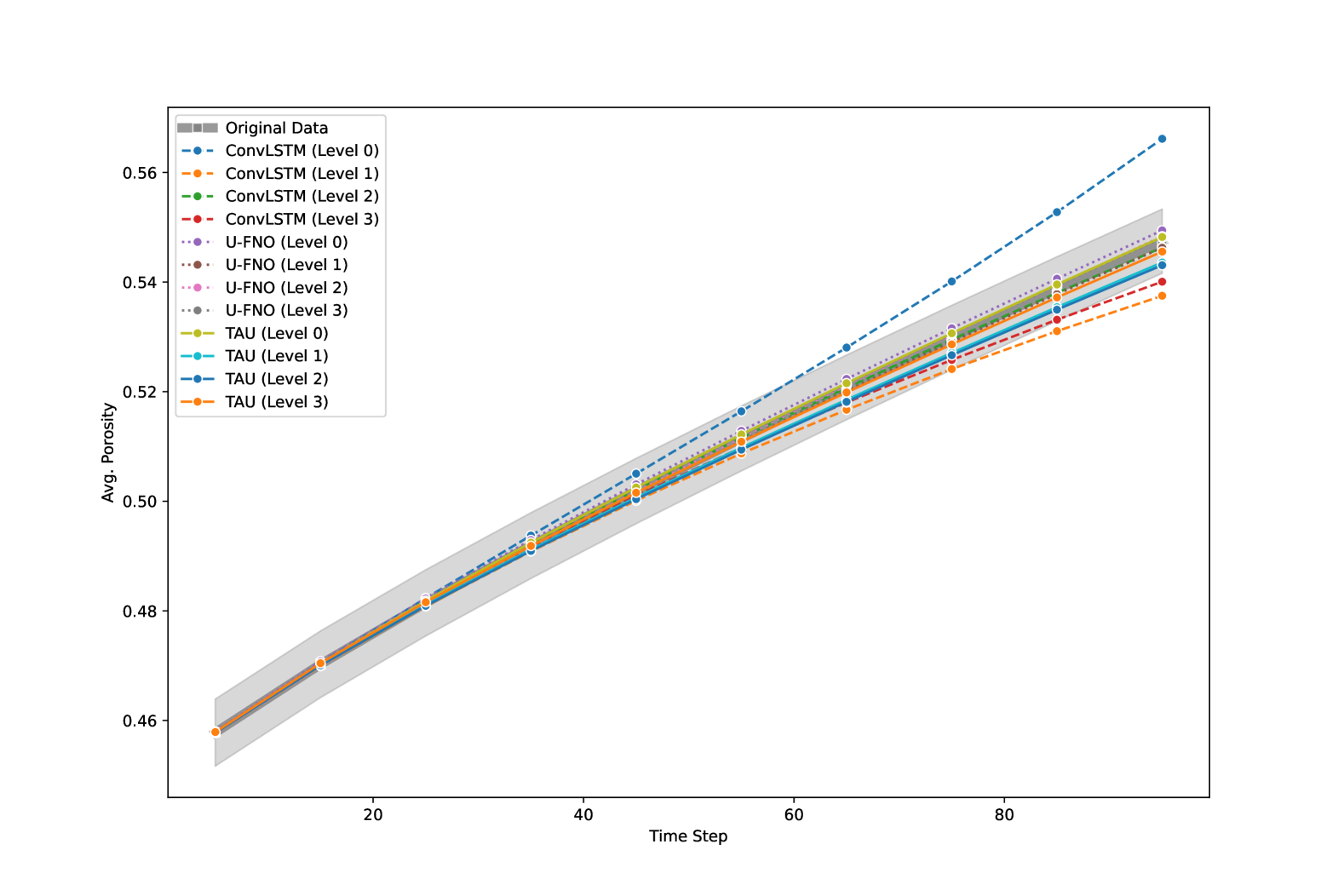
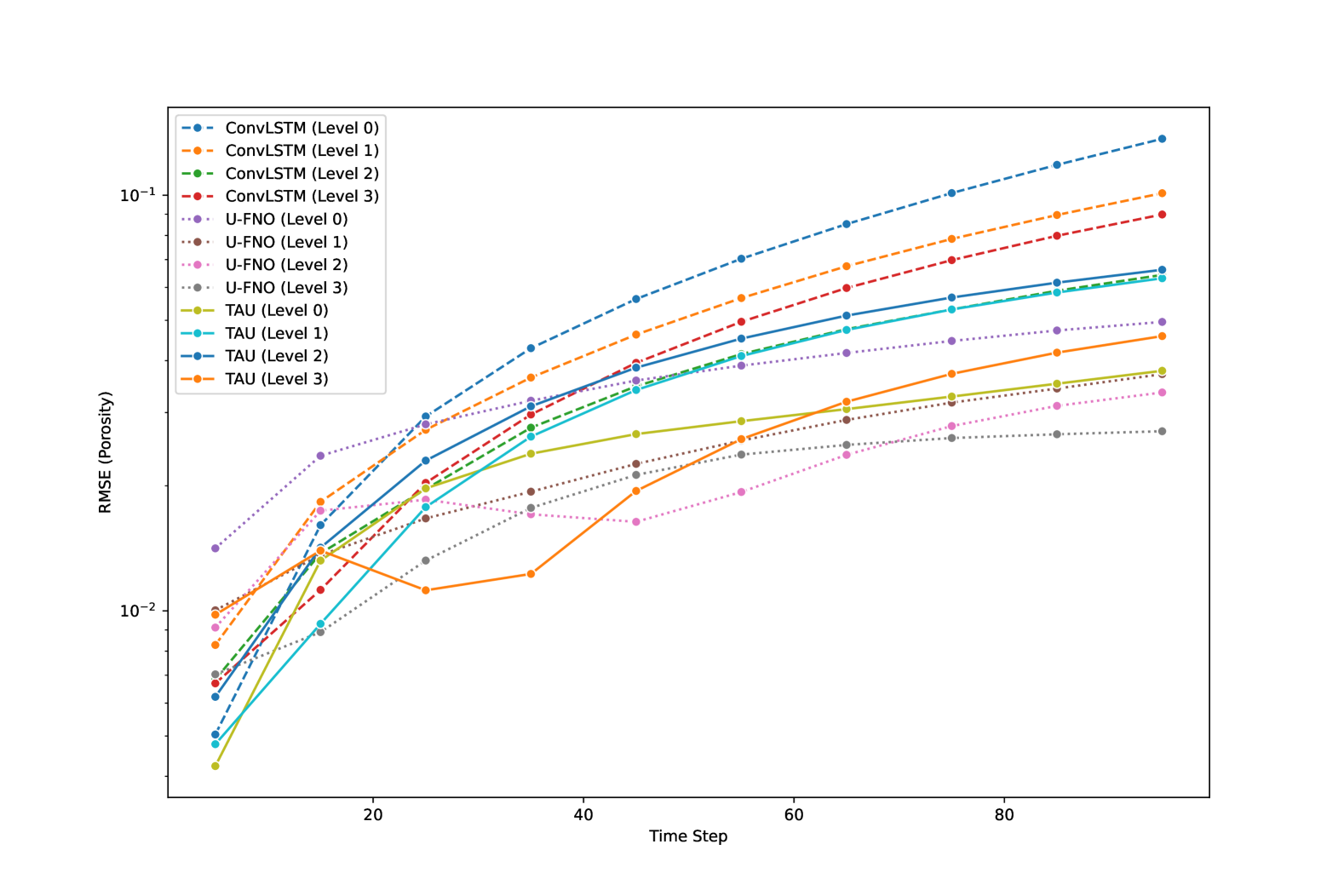
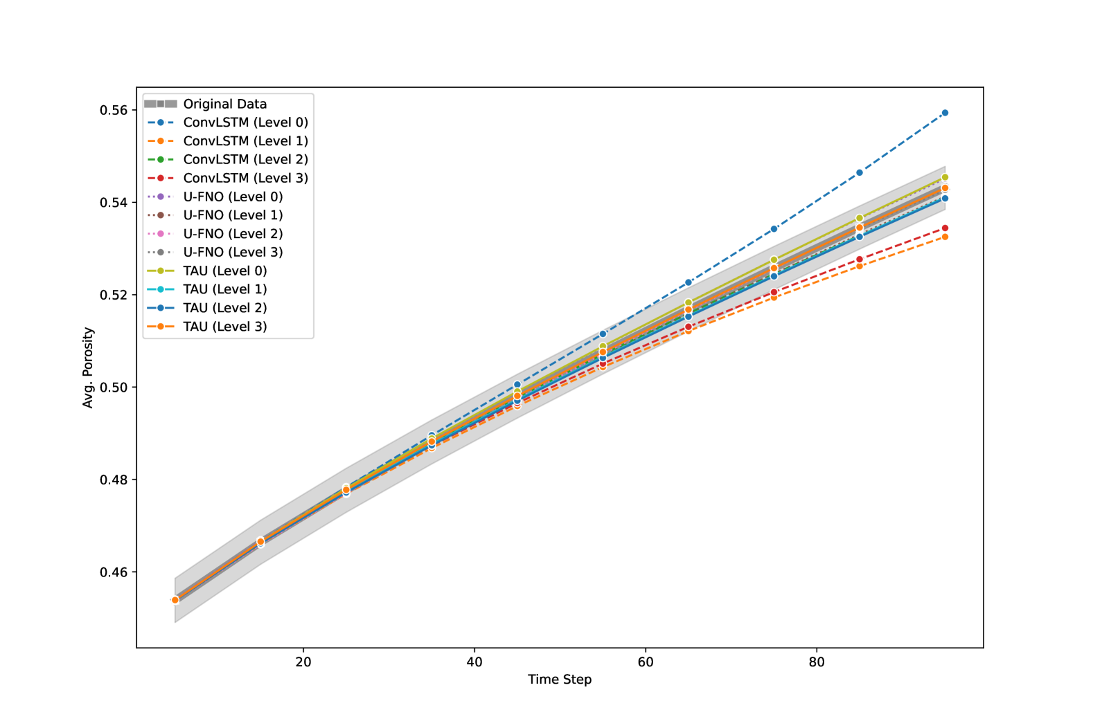
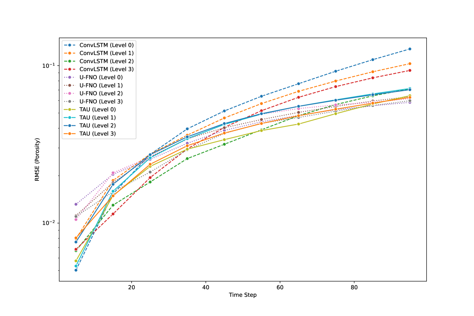
For the validation set, similar results as the training set are achieved for the average error plots (Figure 12). Here, TAU Level 3 was the closest curve to the ground truth at the end of the dissolution, although the curves from its remaining levels and the ones from U-FNO were slightly farther away, but still constantly lying inside the error interval. Concerning the RMSE plots (Figure 12), we can also notice an error reduction on higher network levels for all algorithms, especially after time step 45. This reduction is more noticeable for ConvLSTM, whose Level 2 network achieved significantly lower results than its Level 0 counterpart, at the same time it yielded the lowest errors between time steps 25 and 55. TAU produced very close results among all levels, where Level 2 achieved the lowest error rates at late time steps, but still being slightly worse than ConvLSTM Level 2. Last, U-FNO showed the highest errors at early time steps (5 to 25), achieving the lowest error rates for late time steps (65 to 95).
5.6.2 Permeability Estimation
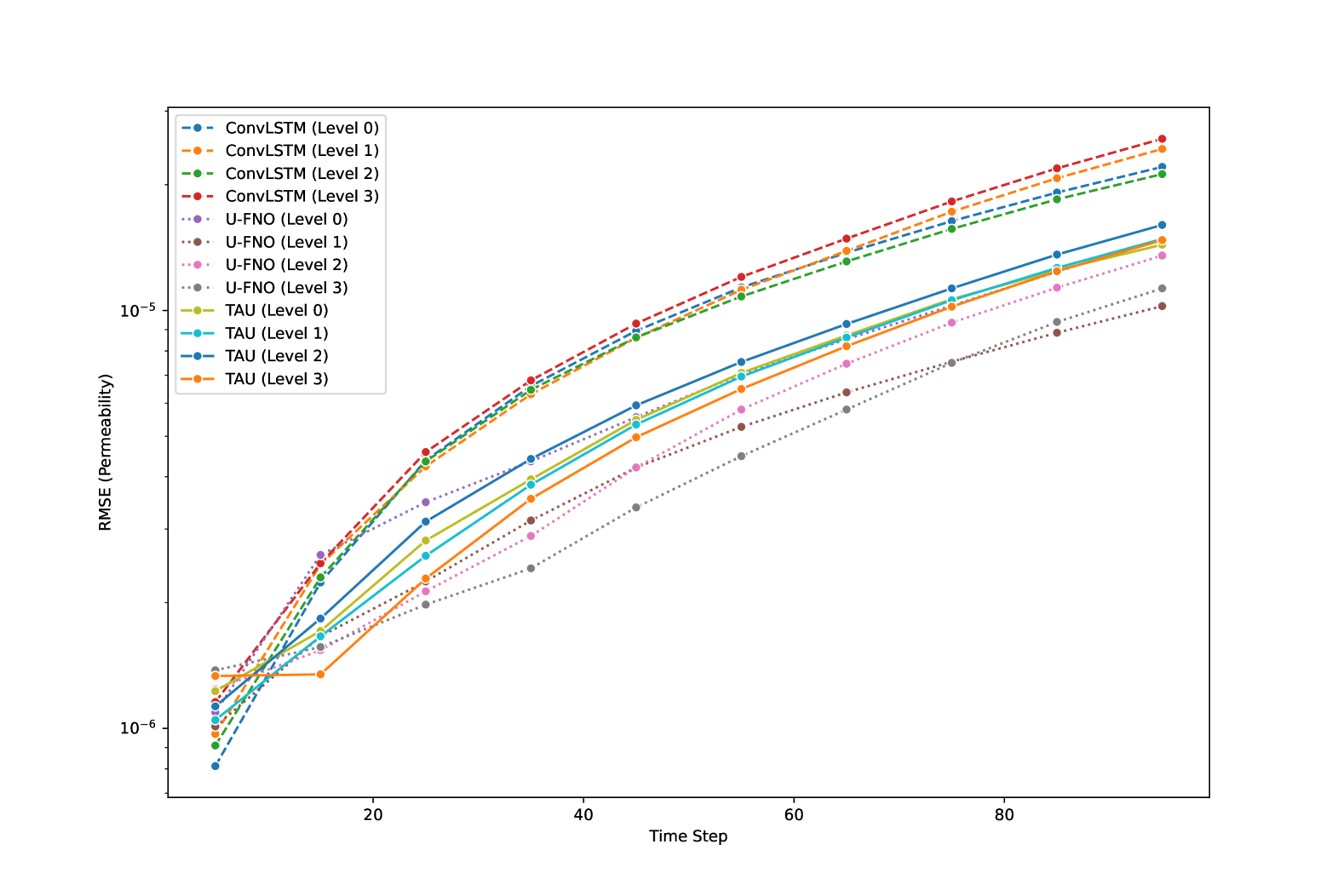
Figure 13 showcases the results for the permeability estimation on the training set. From the curves in both plots, we can observe that the multi-level stacking was not enough to produce a consistent evolution over the levels for all algorithms. This is corroborated by the fact that the closest curves to the ground truth (Figure 13) were obtained from TAU Level 0 and U-FNO Level 0. Moreover, when analyzing the RMSE curves for each algorithm (Figure 13), ConvLSTM Level 3 yielded the worst results during all the dissolution steps. Regarding the TAU curves, the Level 3 network achieved the lowest error rates until the last time step, where the Level 0 network was slightly better. For the U-FNO, the Level 3 network was the best among all networks between time steps 25 and 65, being later surpassed by its Level 1 counterpart.
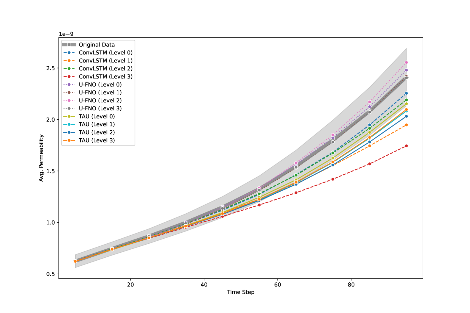
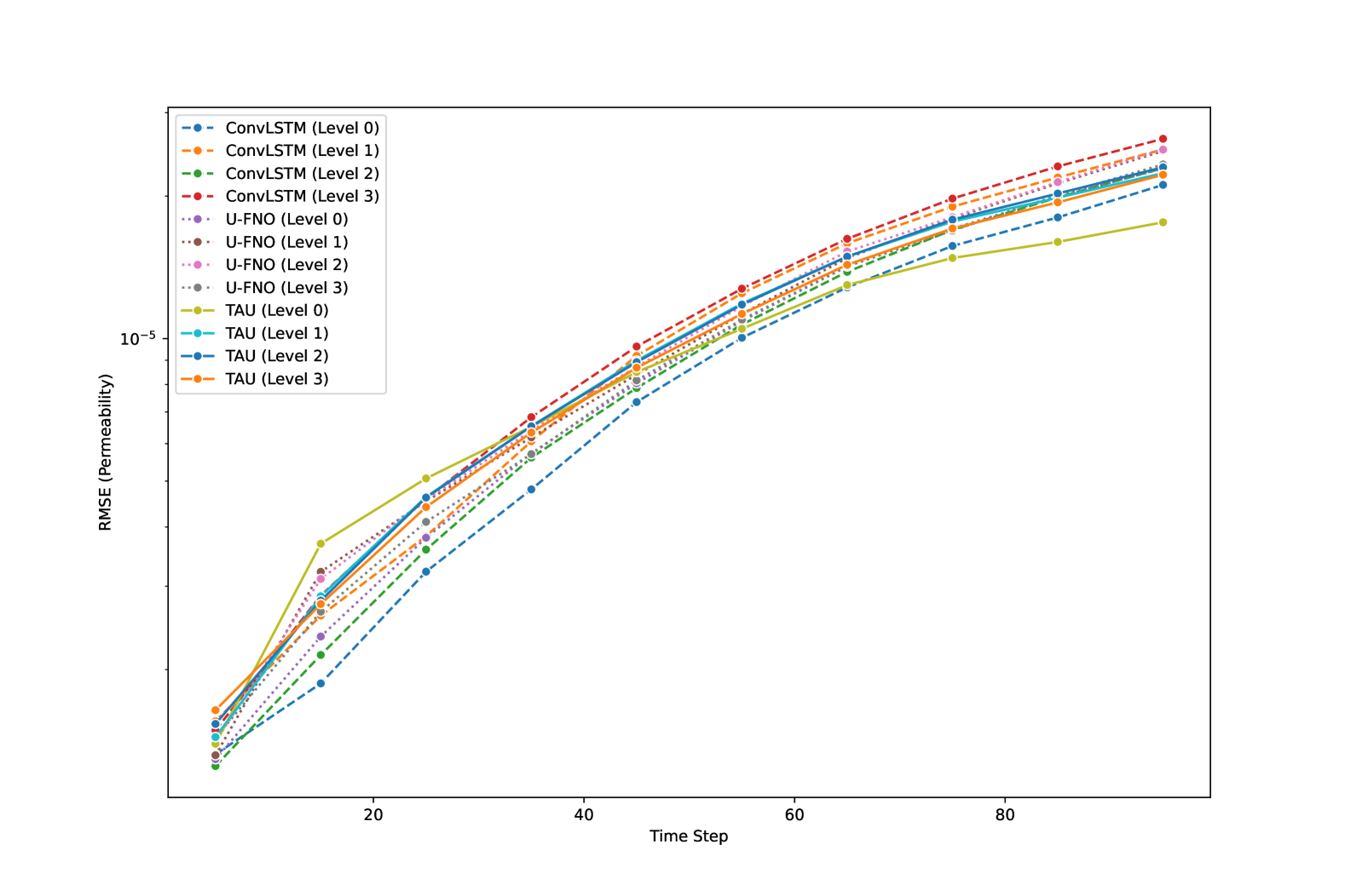
With respect to the estimation on the validation set, the evolution curves from Figure 14 show that the U-FNO curves were the closest ones to the ground truth. Unlike the training set, the TAU curves were farther away from the ground truth, where the Level 0 curve was the only one to remain inside the error margin bounds during all the dissolution. About ConvLSTM, the best results were achieved by its Level 0 network.
Considering the RMSE curves from Figure 14, the lowest errors were achieved by ConvLSTM Level 0 (time steps 15 to 45) and TAU Level 0 (time steps 55 to 95). Furthermore, ConvLSTM Level 3 produced the highest errors between time steps 45 to 95. For the same interval, U-FNO Level 3 achieved the lowest results among all its levels, although still being slightly worse than TAU Level 0.
6 Conclusions
This paper presented a data-driven method that leverages deep learning methods to predict the evolution in time of reactive dissolution in porous media. An iterative stacked MIMO approach was adopted to produce the future states of a dissolution process, starting with an initial set of ”perfect” inputs, generating an output which is then used as input to predict the subsequent states, and so on. To mitigate the overall errors of the predictions, a multi-level stacking approach was proposed, where each level is trained to correct the errors produced by the previous level network. Three different algorithms (ConvLSTM, U-FNO and TAU) were tested in a dataset comprised of 32 numerical simulation models.
Although error accumulation in recursive strategies for prediction of time-series data is still an open problem, all algorithms showed high correlation scores, especially regarding the predictions of and , even at late time steps. Moreover, the multi-stacking approach was successful at improving the results from the base model (Level 0) of each algorithm for the majority of the cases. On the other hand, TAU did not benefit so much from this pipeline, which emphasizes the need for further investigation on the weight of the regularization term of its loss function. Even so, its Level 0 network was capable of achieving higher correlations than the other algorithms (and their corrections) for all predicted properties (except ), at the same time it achieved faster training and forward times.
Despite the high correlation scores for prediction, there is still some improvement possible in estimating bulk properties from the predicted maps, which would bridge the gap between pore-scale interactions and macroscopic flow and transport behaviors, and provide a broader understanding of such phenomena in a porous medium. This is particularly true when assessing the error rates for porosity and permeability estimation, which were expected to decrease over each network level, following similar patterns to the correlation plots. However, as none of the networks was calibrated to be aware of the overall bulk properties at a given time step, the evolution of those error rates ended up showing an uncorrelated pattern to the predictions. Nevertheless, all algorithms managed to produce low-magnitude error rates for porosity and permeability, and similar evolutions to their respective ground truths, considering an ”average pore geometry” across all samples from our dataset. Hence, our method has a potential to replace traditional numerical solvers, especially when also taking into account the reported speedup and lowered computational expense.
Future directions for this work include: 1) analysis of gradient accumulation to improve iterative predictions at late time steps; 2) in-depth study of bulk property estimation; 3) application of the proposed method in larger-scale domains.
7 Acknowledgements
This work is funded by the Engineering and Physical Sciences Research Council’s ECO-AI Project grant (reference number EP/Y006143/1), with additional financial support from the PETRONAS Centre of Excellence in Subsurface Engineering and Energy Transition (PACESET).
Appendix A Mean Squared Error (MSE) Scores for Iterative Prediction
To quantify the error magnitudes of the iterative predictions, we also conducted an analysis of the evolution of MSE scores. Figures 15 and 16 show the MSE scores of the iterative predictions on the training and validation sets, respectively. Compared to the results discussed in Section 5.3, the ranking of all methods on both scenarios remained the same as the ones produced by the PCC metric. These results indicate that TAU not only has a higher linear relationship to the ground truth, but also yields the smallest errors on its predictions among the tested algorithms.
Acknowledgements.
This work is funded by the Engineering and Physical Sciences Research Council’s ECO-AI Project grant (reference number EP/Y006143/1), with additional financial support from the PETRONAS Centre of Excellence in Subsurface Engineering and Energy Transition (PACESET).References
- Alqahtani \BOthers. (\APACyear2018) \APACinsertmetastaralqahtani2018deep{APACrefauthors}Alqahtani, N., Armstrong, R\BPBIT.\BCBL \BBA Mostaghimi, P. \APACrefYearMonthDay2018. \BBOQ\APACrefatitleDeep learning convolutional neural networks to predict porous media properties Deep learning convolutional neural networks to predict porous media properties.\BBCQ \BIn \APACrefbtitleSPE Asia Pacific Oil and Gas Conference and Exhibition SPE Asia Pacific Oil and Gas Conference and Exhibition (\BPG D012S032R010). \PrintBackRefs\CurrentBib
- Al-Shabandar \BOthers. (\APACyear2021) \APACinsertmetastaral2021deep{APACrefauthors}Al-Shabandar, R., Jaddoa, A., Liatsis, P.\BCBL \BBA Hussain, A\BPBIJ. \APACrefYearMonthDay2021. \BBOQ\APACrefatitleA deep gated recurrent neural network for petroleum production forecasting A deep gated recurrent neural network for petroleum production forecasting.\BBCQ \APACjournalVolNumPagesMachine Learning with Applications3100013. \PrintBackRefs\CurrentBib
- Bahdanau (\APACyear2014) \APACinsertmetastarbahdanau2014neural{APACrefauthors}Bahdanau, D. \APACrefYearMonthDay2014. \BBOQ\APACrefatitleNeural machine translation by jointly learning to align and translate Neural machine translation by jointly learning to align and translate.\BBCQ \APACjournalVolNumPagesarXiv preprint arXiv:1409.0473. \PrintBackRefs\CurrentBib
- Cheng \BOthers. (\APACyear2023) \APACinsertmetastarcheng2023ensemble{APACrefauthors}Cheng, M., Fang, F., Navon, I\BPBIM.\BCBL \BBA Pain, C. \APACrefYearMonthDay2023. \BBOQ\APACrefatitleEnsemble Kalman filter for GAN-ConvLSTM based long lead-time forecasting Ensemble Kalman filter for GAN-ConvLSTM based long lead-time forecasting.\BBCQ \APACjournalVolNumPagesJournal of Computational Science69102024. \PrintBackRefs\CurrentBib
- Da Wang \BOthers. (\APACyear2021) \APACinsertmetastarda2021deep{APACrefauthors}Da Wang, Y., Blunt, M\BPBIJ., Armstrong, R\BPBIT.\BCBL \BBA Mostaghimi, P. \APACrefYearMonthDay2021. \BBOQ\APACrefatitleDeep learning in pore scale imaging and modeling Deep learning in pore scale imaging and modeling.\BBCQ \APACjournalVolNumPagesEarth-Science Reviews215103555. \PrintBackRefs\CurrentBib
- Ding \BOthers. (\APACyear2022) \APACinsertmetastarding2022low{APACrefauthors}Ding, C., Zhou, Y., Pu, G.\BCBL \BBA Zhang, H. \APACrefYearMonthDay2022. \BBOQ\APACrefatitleLow carbon economic dispatch of power system at multiple time scales considering GRU wind power forecasting and integrated carbon capture Low carbon economic dispatch of power system at multiple time scales considering GRU wind power forecasting and integrated carbon capture.\BBCQ \APACjournalVolNumPagesFrontiers in Energy Research10953883. \PrintBackRefs\CurrentBib
- Du \BOthers. (\APACyear2023) \APACinsertmetastardu2023modeling{APACrefauthors}Du, H., Zhao, Z., Cheng, H., Yan, J.\BCBL \BBA He, Q. \APACrefYearMonthDay2023. \BBOQ\APACrefatitleModeling density-driven flow in porous media by physics-informed neural networks for CO2 sequestration Modeling density-driven flow in porous media by physics-informed neural networks for CO2 sequestration.\BBCQ \APACjournalVolNumPagesComputers and Geotechnics159105433. \PrintBackRefs\CurrentBib
- Esfe \BBA Esfandeh (\APACyear2020) \APACinsertmetastaresfe20203d{APACrefauthors}Esfe, M\BPBIH.\BCBT \BBA Esfandeh, S. \APACrefYearMonthDay2020. \BBOQ\APACrefatitle3D numerical simulation of the enhanced oil recovery process using nanoscale colloidal solution flooding 3D numerical simulation of the enhanced oil recovery process using nanoscale colloidal solution flooding.\BBCQ \APACjournalVolNumPagesJournal of Molecular Liquids301112094. \PrintBackRefs\CurrentBib
- Feng \BOthers. (\APACyear2024) \APACinsertmetastarfeng2024encoder{APACrefauthors}Feng, Z., Tariq, Z., Shen, X., Yan, B., Tang, X.\BCBL \BBA Zhang, F. \APACrefYearMonthDay2024. \BBOQ\APACrefatitleAn encoder-decoder ConvLSTM surrogate model for simulating geological CO2 sequestration with dynamic well controls An encoder-decoder ConvLSTM surrogate model for simulating geological CO2 sequestration with dynamic well controls.\BBCQ \APACjournalVolNumPagesGas Science and Engineering125205314. \PrintBackRefs\CurrentBib
- Gao \BOthers. (\APACyear2022) \APACinsertmetastargao2022simvp{APACrefauthors}Gao, Z., Tan, C., Wu, L.\BCBL \BBA Li, S\BPBIZ. \APACrefYearMonthDay2022. \BBOQ\APACrefatitleSimVP: Simpler yet better video prediction SimVP: Simpler yet better video prediction.\BBCQ \BIn \APACrefbtitleProceedings of the IEEE/CVF Conference on Computer Vision and Pattern Recognition Proceedings of the IEEE/CVF Conference on Computer Vision and Pattern Recognition (\BPGS 3170–3180). \PrintBackRefs\CurrentBib
- Garnier \BOthers. (\APACyear2021) \APACinsertmetastargarnier2021review{APACrefauthors}Garnier, P., Viquerat, J., Rabault, J., Larcher, A., Kuhnle, A.\BCBL \BBA Hachem, E. \APACrefYearMonthDay2021. \BBOQ\APACrefatitleA review on deep reinforcement learning for fluid mechanics A review on deep reinforcement learning for fluid mechanics.\BBCQ \APACjournalVolNumPagesComputers & Fluids225104973. \PrintBackRefs\CurrentBib
- Graczyk \BBA Matyka (\APACyear2020) \APACinsertmetastargraczyk2020predicting{APACrefauthors}Graczyk, K\BPBIM.\BCBT \BBA Matyka, M. \APACrefYearMonthDay2020. \BBOQ\APACrefatitlePredicting porosity, permeability, and tortuosity of porous media from images by deep learning Predicting porosity, permeability, and tortuosity of porous media from images by deep learning.\BBCQ \APACjournalVolNumPagesScientific Reports10121488. \PrintBackRefs\CurrentBib
- He \BOthers. (\APACyear2020) \APACinsertmetastarhe2020physics{APACrefauthors}He, Q., Barajas-Solano, D., Tartakovsky, G.\BCBL \BBA Tartakovsky, A\BPBIM. \APACrefYearMonthDay2020. \BBOQ\APACrefatitlePhysics-informed neural networks for multiphysics data assimilation with application to subsurface transport Physics-informed neural networks for multiphysics data assimilation with application to subsurface transport.\BBCQ \APACjournalVolNumPagesAdvances in Water Resources141103610. \PrintBackRefs\CurrentBib
- Heinemann \BOthers. (\APACyear2021) \APACinsertmetastarheinemann2021enabling{APACrefauthors}Heinemann, N., Alcalde, J., Miocic, J\BPBIM., Hangx, S\BPBIJ\BPBIT., Kallmeyer, J., Ostertag-Henning, C.\BDBLRudloff, A. \APACrefYearMonthDay2021. \BBOQ\APACrefatitleEnabling large-scale hydrogen storage in porous media–the scientific challenges Enabling large-scale hydrogen storage in porous media–the scientific challenges.\BBCQ \APACjournalVolNumPagesEnergy & Environmental Science142853–864. \PrintBackRefs\CurrentBib
- Kakka (\APACyear2022) \APACinsertmetastarkakka2022sequence{APACrefauthors}Kakka, P\BPBIR. \APACrefYearMonthDay2022. \BBOQ\APACrefatitleSequence to sequence AE-ConvLSTM network for modelling the dynamics of PDE systems Sequence to sequence AE-ConvLSTM network for modelling the dynamics of PDE systems.\BBCQ \APACjournalVolNumPagesarXiv preprint arXiv:2208.07315. \PrintBackRefs\CurrentBib
- Kani \BBA Elsheikh (\APACyear2017) \APACinsertmetastarkani2017dr{APACrefauthors}Kani, J\BPBIN.\BCBT \BBA Elsheikh, A\BPBIH. \APACrefYearMonthDay2017. \BBOQ\APACrefatitleDR-RNN: A deep residual recurrent neural network for model reduction DR-RNN: A deep residual recurrent neural network for model reduction.\BBCQ \APACjournalVolNumPagesarXiv preprint arXiv:1709.00939. \PrintBackRefs\CurrentBib
- Karimi \BBA Bhattacharya (\APACyear2024) \APACinsertmetastarkarimi2024learning{APACrefauthors}Karimi, M.\BCBT \BBA Bhattacharya, K. \APACrefYearMonthDay2024. \BBOQ\APACrefatitleA learning-based multiscale model for reactive flow in porous media A learning-based multiscale model for reactive flow in porous media.\BBCQ \APACjournalVolNumPagesWater Resources Research609. \PrintBackRefs\CurrentBib
- Khebzegga \BOthers. (\APACyear2020) \APACinsertmetastarkhebzegga2020continuous{APACrefauthors}Khebzegga, O., Iranshahr, A.\BCBL \BBA Tchelepi, H. \APACrefYearMonthDay2020. \BBOQ\APACrefatitleContinuous relative permeability model for compositional simulation Continuous relative permeability model for compositional simulation.\BBCQ \APACjournalVolNumPagesTransport in Porous Media134139–172. \PrintBackRefs\CurrentBib
- Kingma (\APACyear2014) \APACinsertmetastarkingma2014adam{APACrefauthors}Kingma, D\BPBIP. \APACrefYearMonthDay2014. \BBOQ\APACrefatitleAdam: A method for stochastic optimization Adam: A method for stochastic optimization.\BBCQ \APACjournalVolNumPagesarXiv preprint arXiv:1412.6980. \PrintBackRefs\CurrentBib
- Kochkov \BOthers. (\APACyear2021) \APACinsertmetastarkochkov2021machine{APACrefauthors}Kochkov, D., Smith, J\BPBIA., Alieva, A., Wang, Q., Brenner, M\BPBIP.\BCBL \BBA Hoyer, S. \APACrefYearMonthDay2021. \BBOQ\APACrefatitleMachine learning–accelerated computational fluid dynamics Machine learning–accelerated computational fluid dynamics.\BBCQ \APACjournalVolNumPagesProceedings of the National Academy of Sciences11821e2101784118. \PrintBackRefs\CurrentBib
- Koesdwiady \BOthers. (\APACyear2018) \APACinsertmetastarkoesdwiady2018methods{APACrefauthors}Koesdwiady, A., El Khatib, A.\BCBL \BBA Karray, F. \APACrefYearMonthDay2018. \BBOQ\APACrefatitleMethods to improve multi-step time series prediction Methods to improve multi-step time series prediction.\BBCQ \BIn \APACrefbtitle2018 International Joint Conference on Neural Networks (IJCNN) 2018 International Joint Conference on Neural Networks (IJCNN) (\BPGS 1–8). \PrintBackRefs\CurrentBib
- A. Li \BOthers. (\APACyear2020) \APACinsertmetastarli2020reaction{APACrefauthors}Li, A., Chen, R., Farimani, A\BPBIB.\BCBL \BBA Zhang, Y\BPBIJ. \APACrefYearMonthDay2020. \BBOQ\APACrefatitleReaction diffusion system prediction based on convolutional neural network Reaction diffusion system prediction based on convolutional neural network.\BBCQ \APACjournalVolNumPagesScientific Reports1013894. \PrintBackRefs\CurrentBib
- Z. Li \BOthers. (\APACyear2020) \APACinsertmetastarli2020fourier{APACrefauthors}Li, Z., Kovachki, N., Azizzadenesheli, K., Liu, B., Bhattacharya, K., Stuart, A.\BCBL \BBA Anandkumar, A. \APACrefYearMonthDay2020. \BBOQ\APACrefatitleFourier neural operator for parametric partial differential equations Fourier neural operator for parametric partial differential equations.\BBCQ \APACjournalVolNumPagesarXiv preprint arXiv:2010.08895. \PrintBackRefs\CurrentBib
- Liang \BOthers. (\APACyear2021) \APACinsertmetastarliang2021review{APACrefauthors}Liang, S\BHBIY., Lin, W\BHBIS., Chen, C\BHBIP., Liu, C\BHBIW.\BCBL \BBA Fan, C. \APACrefYearMonthDay2021. \BBOQ\APACrefatitleA review of geochemical modeling for the performance assessment of radioactive waste disposal in a subsurface system A review of geochemical modeling for the performance assessment of radioactive waste disposal in a subsurface system.\BBCQ \APACjournalVolNumPagesApplied Sciences11135879. \PrintBackRefs\CurrentBib
- Lim \BBA Zohren (\APACyear2021) \APACinsertmetastarlim2021time{APACrefauthors}Lim, B.\BCBT \BBA Zohren, S. \APACrefYearMonthDay2021. \BBOQ\APACrefatitleTime-series forecasting with deep learning: a survey Time-series forecasting with deep learning: a survey.\BBCQ \APACjournalVolNumPagesPhilosophical Transactions of the Royal Society A379219420200209. \PrintBackRefs\CurrentBib
- Maes \BOthers. (\APACyear2022) \APACinsertmetastarmaes2022improved{APACrefauthors}Maes, J., Soulaine, C.\BCBL \BBA Menke, H\BPBIP. \APACrefYearMonthDay2022. \BBOQ\APACrefatitleImproved volume-of-solid formulations for micro-continuum simulation of mineral dissolution at the pore-scale Improved volume-of-solid formulations for micro-continuum simulation of mineral dissolution at the pore-scale.\BBCQ \APACjournalVolNumPagesFrontiers in Earth Science10917931. \PrintBackRefs\CurrentBib
- Makridakis \BOthers. (\APACyear2018) \APACinsertmetastarmakridakis2018statistical{APACrefauthors}Makridakis, S., Spiliotis, E.\BCBL \BBA Assimakopoulos, V. \APACrefYearMonthDay2018. \BBOQ\APACrefatitleStatistical and Machine Learning forecasting methods: Concerns and ways forward Statistical and machine learning forecasting methods: Concerns and ways forward.\BBCQ \APACjournalVolNumPagesPloS One133e0194889. \PrintBackRefs\CurrentBib
- Mohajerin \BBA Waslander (\APACyear2019) \APACinsertmetastarmohajerin2019multistep{APACrefauthors}Mohajerin, N.\BCBT \BBA Waslander, S\BPBIL. \APACrefYearMonthDay2019. \BBOQ\APACrefatitleMultistep prediction of dynamic systems with recurrent neural networks Multistep prediction of dynamic systems with recurrent neural networks.\BBCQ \APACjournalVolNumPagesIEEE Transactions on Neural Networks and Learning Systems30113370–3383. \PrintBackRefs\CurrentBib
- MS \BBA Menon (\APACyear2021) \APACinsertmetastarms2021measuring{APACrefauthors}MS, M., Vishnu Mohan\BCBT \BBA Menon, V. \APACrefYearMonthDay2021. \BBOQ\APACrefatitleMeasuring viscosity of fluids: a deep learning approach using a CNN-RNN architecture Measuring viscosity of fluids: a deep learning approach using a CNN-RNN architecture.\BBCQ \BIn \APACrefbtitleProceedings of the First International Conference on AI-ML Systems Proceedings of the first international conference on ai-ml systems (\BPGS 1–5). \PrintBackRefs\CurrentBib
- Nguyen \BOthers. (\APACyear2023) \APACinsertmetastarnguyen2023scaling{APACrefauthors}Nguyen, T., Shah, R., Bansal, H., Arcomano, T., Madireddy, S., Maulik, R.\BDBLGrover, A. \APACrefYearMonthDay2023. \BBOQ\APACrefatitleScaling transformer neural networks for skillful and reliable medium-range weather forecasting Scaling transformer neural networks for skillful and reliable medium-range weather forecasting.\BBCQ \APACjournalVolNumPagesarXiv preprint arXiv:2312.03876. \PrintBackRefs\CurrentBib
- Oprea \BOthers. (\APACyear2020) \APACinsertmetastaroprea2020review{APACrefauthors}Oprea, S., Martinez-Gonzalez, P., Garcia-Garcia, A., Castro-Vargas, J\BPBIA., Orts-Escolano, S., Garcia-Rodriguez, J.\BCBL \BBA Argyros, A. \APACrefYearMonthDay2020. \BBOQ\APACrefatitleA review on deep learning techniques for video prediction A review on deep learning techniques for video prediction.\BBCQ \APACjournalVolNumPagesIEEE Transactions on Pattern Analysis and Machine Intelligence4462806–2826. \PrintBackRefs\CurrentBib
- Raissi \BOthers. (\APACyear2019) \APACinsertmetastarraissi2019physics{APACrefauthors}Raissi, M., Perdikaris, P.\BCBL \BBA Karniadakis, G\BPBIE. \APACrefYearMonthDay2019. \BBOQ\APACrefatitlePhysics-informed neural networks: A deep learning framework for solving forward and inverse problems involving nonlinear partial differential equations Physics-informed neural networks: A deep learning framework for solving forward and inverse problems involving nonlinear partial differential equations.\BBCQ \APACjournalVolNumPagesJournal of Computational Physics378686–707. \PrintBackRefs\CurrentBib
- Reichstein \BOthers. (\APACyear2019) \APACinsertmetastarreichstein2019deep{APACrefauthors}Reichstein, M., Camps-Valls, G., Stevens, B., Jung, M., Denzler, J., Carvalhais, N.\BCBL \BBA Prabhat. \APACrefYearMonthDay2019. \BBOQ\APACrefatitleDeep learning and process understanding for data-driven Earth system science Deep learning and process understanding for data-driven Earth system science.\BBCQ \APACjournalVolNumPagesNature5667743195–204. \PrintBackRefs\CurrentBib
- Salimzadeh \BBA Nick (\APACyear2019) \APACinsertmetastarsalimzadeh2019coupled{APACrefauthors}Salimzadeh, S.\BCBT \BBA Nick, H. \APACrefYearMonthDay2019. \BBOQ\APACrefatitleA coupled model for reactive flow through deformable fractures in enhanced geothermal systems A coupled model for reactive flow through deformable fractures in enhanced geothermal systems.\BBCQ \APACjournalVolNumPagesGeothermics8188–100. \PrintBackRefs\CurrentBib
- Santos \BOthers. (\APACyear2020) \APACinsertmetastarsantos2020poreflow{APACrefauthors}Santos, J\BPBIE., Xu, D., Jo, H., Landry, C\BPBIJ., Prodanović, M.\BCBL \BBA Pyrcz, M\BPBIJ. \APACrefYearMonthDay2020. \BBOQ\APACrefatitlePoreFlow-Net: A 3D convolutional neural network to predict fluid flow through porous media PoreFlow-Net: A 3D convolutional neural network to predict fluid flow through porous media.\BBCQ \APACjournalVolNumPagesAdvances in Water Resources138103539. \PrintBackRefs\CurrentBib
- Shi \BOthers. (\APACyear2015) \APACinsertmetastarshi2015convolutional{APACrefauthors}Shi, X., Chen, Z., Wang, H., Yeung, D\BHBIY., Wong, W\BHBIK.\BCBL \BBA Woo, W\BHBIc. \APACrefYearMonthDay2015. \BBOQ\APACrefatitleConvolutional LSTM network: A machine learning approach for precipitation nowcasting Convolutional LSTM network: A machine learning approach for precipitation nowcasting.\BBCQ \APACjournalVolNumPagesAdvances in Neural Information Processing Systems28. \PrintBackRefs\CurrentBib
- Sutskever \BOthers. (\APACyear2014) \APACinsertmetastarsutskever2014sequence{APACrefauthors}Sutskever, I., Vinyals, O.\BCBL \BBA Le, Q\BPBIV. \APACrefYearMonthDay2014. \BBOQ\APACrefatitleSequence to Sequence Learning with Neural Networks Sequence to Sequence Learning with Neural Networks.\BBCQ \APACjournalVolNumPagesarXiv preprint arXiv:1409.3215. \PrintBackRefs\CurrentBib
- Taieb \BOthers. (\APACyear2012) \APACinsertmetastartaieb2012review{APACrefauthors}Taieb, S\BPBIB., Bontempi, G., Atiya, A\BPBIF.\BCBL \BBA Sorjamaa, A. \APACrefYearMonthDay2012. \BBOQ\APACrefatitleA review and comparison of strategies for multi-step ahead time series forecasting based on the NN5 forecasting competition A review and comparison of strategies for multi-step ahead time series forecasting based on the NN5 forecasting competition.\BBCQ \APACjournalVolNumPagesExpert Systems with Applications3987067–7083. \PrintBackRefs\CurrentBib
- Tan \BOthers. (\APACyear2023) \APACinsertmetastartan2023temporal{APACrefauthors}Tan, C., Gao, Z., Wu, L., Xu, Y., Xia, J., Li, S.\BCBL \BBA Li, S\BPBIZ. \APACrefYearMonthDay2023. \BBOQ\APACrefatitleTemporal attention unit: Towards efficient spatiotemporal predictive learning Temporal attention unit: Towards efficient spatiotemporal predictive learning.\BBCQ \BIn \APACrefbtitleProceedings of the IEEE/CVF Conference on Computer Vision and Pattern Recognition Proceedings of the IEEE/CVF Conference on Computer Vision and Pattern Recognition (\BPGS 18770–18782). \PrintBackRefs\CurrentBib
- Tang \BOthers. (\APACyear2021) \APACinsertmetastartang2021deep{APACrefauthors}Tang, M., Liu, Y.\BCBL \BBA Durlofsky, L\BPBIJ. \APACrefYearMonthDay2021. \BBOQ\APACrefatitleDeep-learning-based surrogate flow modeling and geological parameterization for data assimilation in 3D subsurface flow Deep-learning-based surrogate flow modeling and geological parameterization for data assimilation in 3D subsurface flow.\BBCQ \APACjournalVolNumPagesComputer Methods in Applied Mechanics and Engineering376113636. \PrintBackRefs\CurrentBib
- Wang \BOthers. (\APACyear2023) \APACinsertmetastarwang2023pore{APACrefauthors}Wang, W., Xie, Q., An, S., Bakhshian, S., Kang, Q., Wang, H.\BDBLYuan, B. \APACrefYearMonthDay2023. \BBOQ\APACrefatitlePore-scale simulation of multiphase flow and reactive transport processes involved in geologic carbon sequestration Pore-scale simulation of multiphase flow and reactive transport processes involved in geologic carbon sequestration.\BBCQ \APACjournalVolNumPagesEarth-Science Reviews104602. \PrintBackRefs\CurrentBib
- Wen \BOthers. (\APACyear2022) \APACinsertmetastarwen2022u{APACrefauthors}Wen, G., Li, Z., Azizzadenesheli, K., Anandkumar, A.\BCBL \BBA Benson, S\BPBIM. \APACrefYearMonthDay2022. \BBOQ\APACrefatitleU-FNO—An enhanced Fourier neural operator-based deep-learning model for multiphase flow U-fno—an enhanced fourier neural operator-based deep-learning model for multiphase flow.\BBCQ \APACjournalVolNumPagesAdvances in Water Resources163104180. \PrintBackRefs\CurrentBib
- Xu \BOthers. (\APACyear2021) \APACinsertmetastarxu2021spatiotemporal{APACrefauthors}Xu, L., Chen, N., Chen, Z., Zhang, C.\BCBL \BBA Yu, H. \APACrefYearMonthDay2021. \BBOQ\APACrefatitleSpatiotemporal forecasting in earth system science: Methods, uncertainties, predictability and future directions Spatiotemporal forecasting in earth system science: Methods, uncertainties, predictability and future directions.\BBCQ \APACjournalVolNumPagesEarth-Science Reviews222103828. \PrintBackRefs\CurrentBib
- Yan \BOthers. (\APACyear2022) \APACinsertmetastaryan2022physics{APACrefauthors}Yan, B., Harp, D\BPBIR., Chen, B.\BCBL \BBA Pawar, R. \APACrefYearMonthDay2022. \BBOQ\APACrefatitleA physics-constrained deep learning model for simulating multiphase flow in 3D heterogeneous porous media A physics-constrained deep learning model for simulating multiphase flow in 3D heterogeneous porous media.\BBCQ \APACjournalVolNumPagesFuel313122693. \PrintBackRefs\CurrentBib
- Zhu \BOthers. (\APACyear2022) \APACinsertmetastarzhu2022review{APACrefauthors}Zhu, L\BHBIT., Chen, X\BHBIZ., Ouyang, B., Yan, W\BHBIC., Lei, H., Chen, Z.\BCBL \BBA Luo, Z\BHBIH. \APACrefYearMonthDay2022. \BBOQ\APACrefatitleReview of machine learning for hydrodynamics, transport, and reactions in multiphase flows and reactors Review of machine learning for hydrodynamics, transport, and reactions in multiphase flows and reactors.\BBCQ \APACjournalVolNumPagesIndustrial & Engineering Chemistry Research61289901–9949. \PrintBackRefs\CurrentBib