Hierarchical Contact-Rich Trajectory Optimization for Multi-Modal Manipulation using Tight Convex Relaxations

Abstract

Designing trajectories for manipulation through contact is challenging as it requires reasoning of object & robot trajectories as well as complex contact sequences simultaneously. In this paper, we present a novel framework for simultaneously designing trajectories of robots, objects, and contacts efficiently for contact-rich manipulation. We propose a hierarchical optimization framework where Mixed-Integer Linear Program (MILP) selects optimal contacts between robot & object using approximate dynamical constraints, and then a NonLinear Program (NLP) optimizes trajectory of the robot(s) and object considering full nonlinear constraints. We present a convex relaxation of bilinear constraints using binary encoding technique such that MILP can provide tighter solutions with better computational complexity. The proposed framework is evaluated on various manipulation tasks where it can reason about complex multi-contact interactions while providing computational advantages. We also demonstrate our framework in hardware experiments using a bimanual robot system. The video summarizing this paper and hardware experiments is found here.

I Introduction

Humans can effortlessly perform dexterous, multi-modal manipulation tasks while reasoning through complex contact configurations to fully use their whole body during manipulation. However, achieving similar dexterous behavior for robots is very difficult [1, 2, 3]. While there are several critical reasons, we point out a few here. First, planners need to consider long-horizon manipulation to achieve multi-modal, complex behavior [4]. This leads to large-scale optimization problems which are difficult to solve. Second, planners need to consider the kinematic, dynamic, and contact constraints of objects and robots simultaneously, resulting in nonlinear, discontinuous constraints that require careful treatment to find meaningful solutions [5, 6]. Considering all possible contact constraints leads to huge computational costs which is undesirable. Consequently, several manipulation planning algorithms consider fixed contact modes which limits the complexity of tasks which can be solved by these algorithms. Our goal in this paper is to overcome some of these shortcomings by considering reasoning over all contact variables (i.e., locations, sticking, slipping, etc.) while being computationally efficient.

We introduce a hierarchical contact-rich trajectory optimization algorithm that considers kinematics, dynamics, and contact constraints while maintaining computational efficiency. In the proposed hierarchical approach, an MIP plans contact locations and forces between the robot(s) and object while considering approximate constraints. We present a convex relaxation of bilinear constraints, which often appears in cross-product computation of moments and complementarity constraints. This allows our MIP formulation to plan trajectories with the tight approximation of nonlinear dynamics. This solution is then passed to an NLP which reasons about the entire manipulation trajectory considering full nonlinear contact constraints. The proposed hierarchical optimization framework can then effectively reason about very complex contact interactions over long planning horizons and can find very rich solutions resulting in multi-modal behavior where a robot can switch between multiple contact points manipulation. This is illustrated through various numerical as well as hardware experiments (see Fig. 1 for an example of a stowing task).

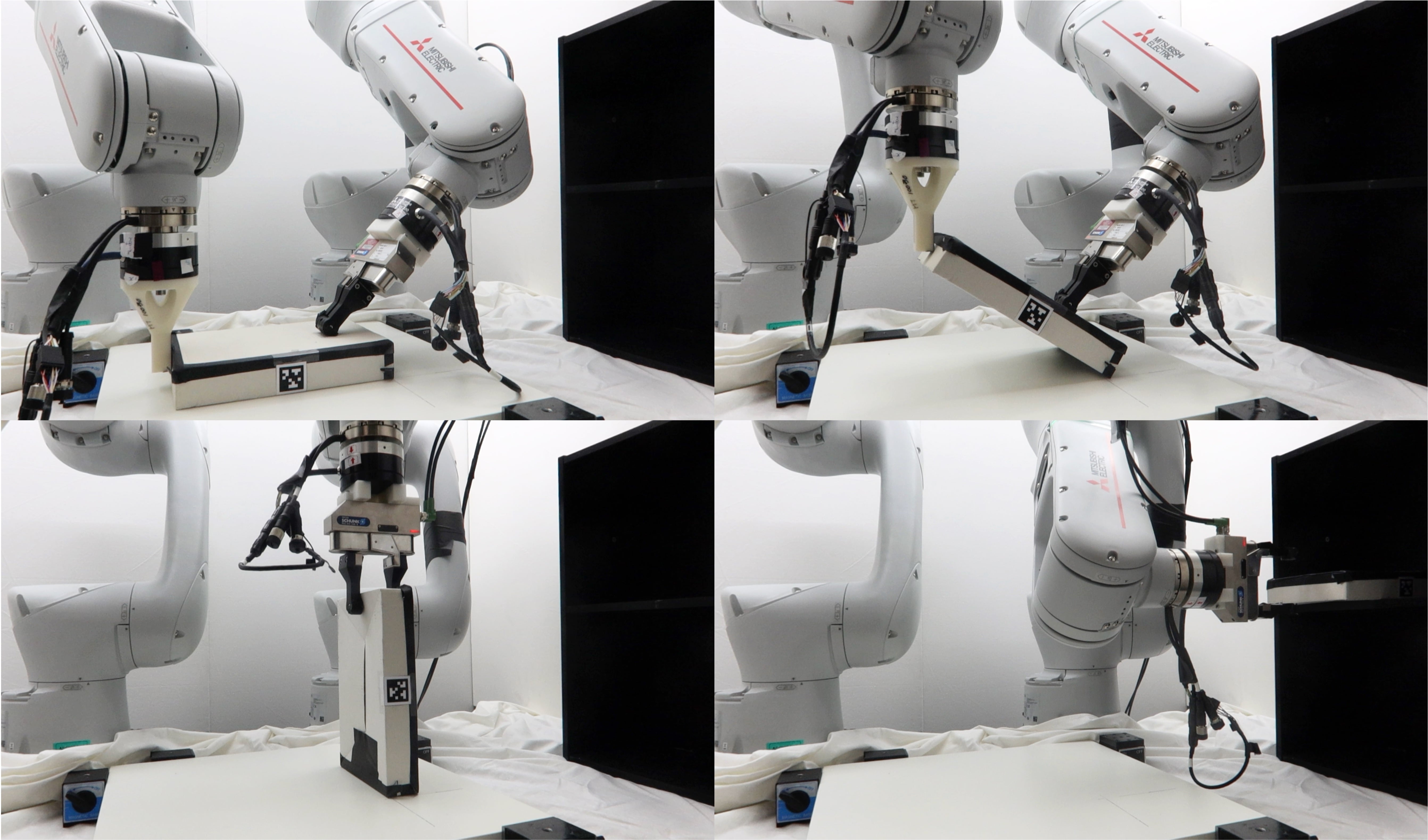
Figure 1: We show a bimanual system which can reason about pivoting the box to grasp it so that it can be stowed on a shelf using the proposed algorithm. The Apriltag system is used for feedback during grasping since the box might slip during pivoting. The hardware experiment video is found here.

Summary of Contributions.

1. We present a framework for simultaneously designing trajectories of robots, an object, and contact efficiently with no fixed contact modes.

2. We propose a tight and efficient convex relaxation of bilinear constraints using the binary encoding method.

3. We extensively verify our approach in multiple manipulation scenarios including hardware experiments.

II Related Work

Contact-Implicit Trajectory Optimization (CITO) has been extensively studied in robotic locomotion and manipulation literature. These works can be based on NLP with complementarity constraints [7, 8, 9, 10, 11], based on MIP [12, 13, 14, 15, 16], or based on smoothed dynamics [17, 18]. Although these works show impressive results, each work has some assumptions on the contact modes (e.g., Sliding-sticking complementarity contact is not considered in [10, 12, 13, 16, 19]. Contact patch is fixed in [7, 9]. Unphysical artifacts, force-at-distance, are introduced in [17].) In [10], the authors present a general-purpose method to consider contact locations between the object and the environment; however, the proposed method can not consider the selection of contact between the robot and the object. In contrast, the framework proposed in this paper does not have any of the aforementioned assumptions.

Another related field is the relaxation of bilinear constraints, which is crucial for improving MIP solution quality. McCormick envelopes provide linear approximations of bilinear terms but can be loose [20]. Quadratic relaxations [13, 21, 22] also struggle to control bilinear violations and require careful tuning. While piecewise McCormick envelopes offer tighter bounds [12, 23], they can be computationally expensive. Instead, we employ binary encoding [24] for a more efficient approach.

III Problem Formulation

We provide an overview of our model and describe the assumptions. We consider the following assumptions.

1. Rigid objects and robots.

2. Quasi-static equilibrium of the system.

3. Manipulation in SE(2).

4. Extrinsic contact happens at the vertices of the object.

The free-body diagram of the system we consider in this work is shown in Fig. 2. In Fig. 2, it is important to point out that an object can make multiple contacts during manipulation. For example, the object can make contact such as extrinsic contact with the environment and the robot contact. For extrinsic contacts, we assume that contacts occur only at the object’s vertices. This is reasonable since other types, like patch contacts, can be approximated by two-point contacts, commonly used in manipulation planning with generalized friction cones [25, 26, 27, 28]. Additionally, this assumption is less restrictive than those in works like [19], which focus solely on tabletop manipulation and the interaction between the robot and the object.

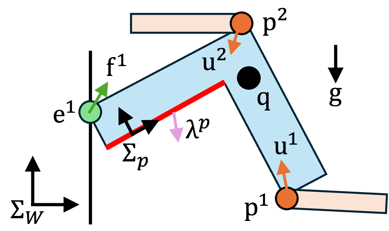
Figure 2: A schematic showing the free-body diagram of a rigid body during manipulation where two robots make contact and there is one extrinsic contact between the object and the environment. We consider $N_{r}=2$, $N_{v}=6$ and $N_{p}=6$ in this figure. The red line represents one specific object’s contact surface with the corresponding local force $\lambda$. The variables in this figure are summarized in Table I.

TABLE I: Notation of variables. C or B indicates the variable is a continuous or binary variable, respectively. In $\Sigma$ column, we indicate the frame of variables. Subscript $t$ indicates time-step.

Name	Description	Size	C/B	$\Sigma$
$\mathbf{q}_{t}$	object pose	$\mathbb{R}^{3}$	C	$W$
$\mathbf{p}_{t}^{i}$	$i$-th robot position	$\mathbb{R}^{2}$	C	$W$
$\mathbf{e}_{t}^{v}$	$v$-th extrinsic contact position	$\mathbb{R}^{2}$	C	$W$
$\mathbf{u}_{t}^{i}$	$i$-th robot contact force	$\mathbb{R}^{2}$	C	$W$
$\boldsymbol{\lambda}^{i,p}_{t}$	$p$-th local force for $i$-th robot	$\mathbb{R}^{2}$	C	$p$
$\mathbf{f}^{v}_{t}$	$v$-th extrinsic contact force	$\mathbb{R}^{2}$	C	$W$
$z^{i,p}_{t}$	$i$-th robot contact at $\mathcal{P}_{p}$	$\mathbb{Z}^{1}$	B

The variables used in this paper are summarized in Table I and Fig. 2. In this work, we consider in total $N_{r}$ robots and a single object which consists of $N_{v}$ potential extrinsic contacts and $N_{p}$ potential object surfaces where the robot can make contact. We denote $\mathcal{P}_{p}$ as the $p$-th object surface, associated with a local frame $\Sigma_{p}$. $\mathcal{P}_{p}$ is represented as halfspace. For any arbitrary vector $\mathbf{x}$, the notation $\|\mathbf{x}\|^{2}_{Q}$ means a quadratic term with a positive-semi-definite matrix $Q$. We define the coordinate transformation and rotation matrix from frame $\Sigma_{A}$ to $\Sigma_{B}$ as ${}^{A}_{B}T$ and ${}^{A}_{B}R$, respectively. We denote $X\Longrightarrow Y$ as a conditional constraint and implement it using a big-M formulation in MIP [29].

The constants $m$ and $\mathbf{g}\in\mathbb{R}^{2}$ represent the mass of the object and gravitational acceleration, defined in world frame $\Sigma_{W}$, respectively. $\mu_{e}^{v}$ and $\mu_{r}^{i}$ are the friction constraints for $v$-th extrinsic contact and $i$-th robot contact, respectively. $h$ is the step size. We use subscripts $n$ and $s$ to represent normal and tangential elements of forces. Also, we use subscripts $x,y,\theta$, to represent the element of $\mathbf{q}_{t}$.

IV Contact-Rich Trajectory Optimization

A naive formulation of trajectory optimization using all possible contact constraints would result in a mixed-integer nonlinear program, which could be computationally very demanding to solve. We propose a method that solves this problem using hierarchical optimization (see Fig. 3).

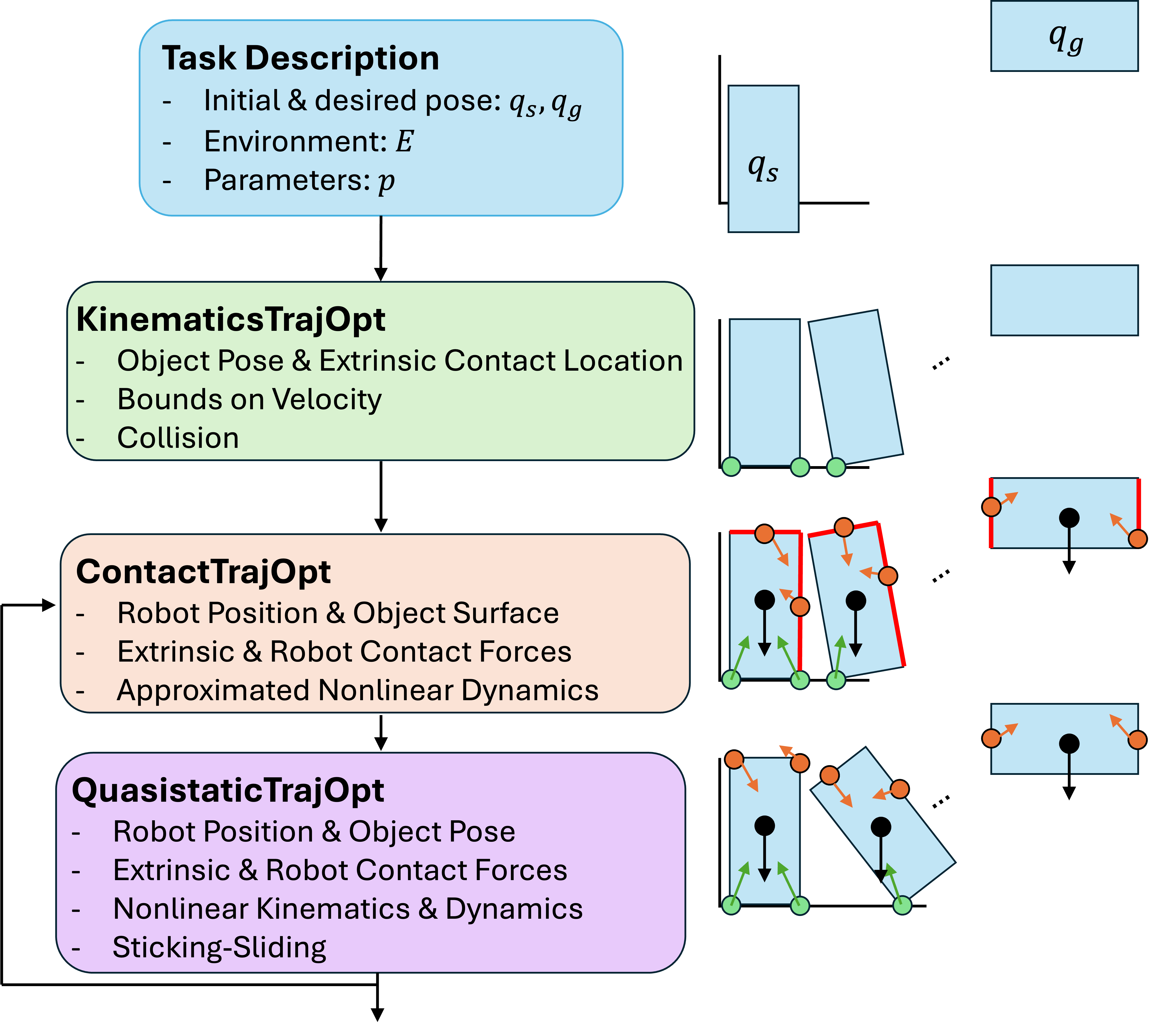
Figure 3: Overview of the proposed framework. See Sec IV-A for details. Orange points and green points represent the robot contact location and extrinsic contact location, respectively. Red lines represent the object’s contact surface where the robot makes contact. We have the cutting plane method to deal with the infeasible solution by Q-Opt (see Sec IV-C).

IV-A Overview

Our framework is illustrated in Fig. 3. Our framework consists of three optimization problems. First, given the task description, Kinematics Trajectory Optimization, K-Opt, finds a feasible trajectory of the pose of the object and extrinsic contacts while satisfying collision constraints between the object and environment. Second, given the solution by K-Opt, Contact Trajectory Optimization, C-Opt, finds a feasible trajectory of extrinsic contact forces, the robot position, and the robot contact force on the contact location between the robot and the object. Finally, using this solution, Quasistatic Trajectory Optimization, Q-Opt, finds a feasible trajectory of the pose of the object, robot position, and the extrinsic & robot contact forces while satisfying full nonlinear dynamic and kinematic constraints. In Q-Opt, the object surface where the robot makes contact is fixed from C-Opt but sliding-sticking complementarity constraints are still considered. Therefore, our method has the flexibility to adjust the robot position such that it can find much richer solutions resulting in more dexterous behavior. It is possible that Q-Opt is unable to find a feasible solution depending on the solution returned by MIP (since MIP considers approximate constraints). In such cases, we remove the specific contact combination from C-Opt and re-run C-Opt based on the cutting-plane method, which is explained in Sec IV-C.

IV-A1 Kinematics Trajectory Optimization

In K-Opt, the goal is to find feasible trajectories of the pose of the object and extrinsic contacts between an object and the environment. We consider the following optimization problem.

$$\min_{\mathbf{q}_{t},\dot{\mathbf{q}}_{t}}\sum_{t=0}^{T}\|\mathbf{q}_{t}-\mathbf{q}_{t}^{\text{ref}}\|^{2}_{Q_{\text{kin}}}$$ (1a)

$$\text{s. t. },\mathbf{q}_{t+1}=\mathbf{q}_{t}+h\dot{\mathbf{q}}_{t}$$ (1b)

$$\underline{\mathbf{q}}_{t}\leq\mathbf{q}_{t}\leq\overline{\mathbf{q}}_{t},\underline{\dot{\mathbf{q}}}_{t}\leq\dot{\mathbf{q}}_{t}\leq\overline{\dot{\mathbf{q}}}_{t},$$ (1c)

$$\text{sdf}(\mathbf{q}_{t})\geq 0,$$ (1d)

where $\mathbf{q}_{t}^{\text{ref}}$ is the linear interpolation between $\mathbf{q}_{\text{s}}$ and $\mathbf{q}_{\text{g}}$ with $T$ steps, and $h$ is time interval. (1b) is the dynamics of object pose and (1c) is the bound of variables. sdf is the signed distance function between the object and the environment which computes the distance between $e_{t}^{v}$ and the environment. None of the constraints in (1) involve any integer variables and thus (1) is formulated as NLP.

After solving (1), we compute a binary map $A$, which tells if each extrinsic contact of the object, $\mathbf{e}_{t}^{v}$, makes contact with the environment, where $\mathbf{e}_{t}^{v}$ is calculated as a function of $\mathbf{q}_{t}$ and the object & environment geometry. Hence, C-Opt does not need to reason about $\mathbf{e}_{t}^{v}$. Similarly, we compute a binary map $B$ to tell which of the extrinsic contacts slip. This helps us consider the correct friction cone constraints for downstream optimization. We denote $x_{\text{kin}}:=[\mathbf{q}_{t},A,B,\forall t]$ to represent the solution from this module.

IV-A2 Contact Trajectory Optimization

In C-Opt, the objective is to find extrinsic contact forces, contact location of the robot, object surfaces where the robot makes contact, and contact forces from the robot for a fixed $x_{\text{kin}}$. The optimization problem is then formulated as:

$$\text{Find}~\mathbf{p}_{t}^{i},\mathbf{u}_{t}^{i},\mathbf{f}_{t}^{v},\boldsymbol{\lambda}^{i,p}_{t},{z}_{t}^{i,p},~\forall t,i,v,p$$ (2a)

$$\text{s. t. },\mathbf{p}_{t+1}=\mathbf{p}_{t}+h\dot{\mathbf{p}}_{t}$$ (2b)

$$\underline{\dot{\mathbf{p}}}_{t}^{i}\leq\dot{\mathbf{p}}_{t}^{i}\leq\overline{\dot{\mathbf{p}}^{i}_{t}},$$ (2c)

$$\mathbf{u}_{t}^{i}=\sum_{p=1}^{N_{p}}{{}^{W}_{p}R}\boldsymbol{\lambda}^{i,p}_{t}$$ (2d)

$$\mathbf{p}_{t}^{i}\in\mathcal{Q}_{\text{surface}}\cap\mathcal{Q}_{\text{mom}}$$ (2e)

$$\boldsymbol{\lambda}^{i,p}_{t}\in\mathcal{Q}_{\text{stable}}\cap\mathcal{Q}_{\text{surface}}\cap\mathcal{Q}_{\text{force}}\cap\mathcal{Q}_{\text{mom}}\cap\mathcal{Q}_{\text{FC}}\cap\mathcal{Q}_{\text{C}}$$ (2f)

$$\mathbf{f}_{t}^{v}\in\mathcal{Q}_{\text{force}}\cap\mathcal{Q}_{\text{mom}}\cap\mathcal{Q}_{\text{FC}}$$ (2g)

$${z}_{t}^{i,p}\in\mathcal{Q}_{\text{surface}}\cap\in\mathcal{Q}_{\text{stable}}\cap\mathcal{Q}_{\text{C}}$$ (2h)

where $\mathcal{Q}_{\text{surface}},\mathcal{Q}_{\text{force}},\mathcal{Q}_{\text{mom}},\mathcal{Q}_{\text{stable}},\mathcal{Q}_{\text{FC}}$, and $\mathcal{Q}_{\text{C}}$ are the set encoding object surface selection constraint, force balance constraint, moment balance constraint, stable contact change constraint, friction cone constant, and integer constraint, respectively. We explain each set in Sec. IV-D. (2b) is the dynamics of the robot position and (2c) considers bound of robot velocity. With (9), (2d) converts a specific local wrench in $\Sigma_{p}$ to the wrench in $\Sigma_{W}$. (2) is a feasibility problem.

In (2), the problem is formulated as mixed-integer non-convex Quadratically Constrained QP (QCQP) due to the bilinear term in $\mathcal{Q}_{\text{mom}}$, which is in general quite tough to find a feasible solution. Thus, we propose a convex relaxation of bilinear terms such that (2) is formulated as MILP, which is much easier to find a feasible solution while improving the computational complexity. After solving C-Opt, C-Opt returns $x_{\text{con}}:=[\mathbf{p}_{t}^{i},\mathbf{u}_{t}^{i},\mathbf{f}_{t}^{v},\boldsymbol{\lambda}^{i,p}_{t},{z}_{t}^{i,p},\forall t,i,v,p]$.

In C-Opt, we do not consider sticking-sliding complementarity constraints. This is mainly for computational reasons. If we consider these constraints in C-Opt, we have many more complicated integer constraints, which makes C-Opt slow. Instead, we propose to let Q-Opt consider sticking-sliding complementarity constraints while making pose of the object, $\mathbf{q}$ as a decision variable. As a result, we can achieve better computation.

Remark. It is possible that K-Opt does not provide a physically feasible $x_{\text{kin}}$ and thus C-Opt finds an infeasible solution. If this happens, we make ${\mathbf{q}}_{t}$ as also part of the decision variable of C-Opt.

IV-A3 Quasi-static Trajectory Optimization

The objective of Q-Opt is to find optimal trajectories of extrinsic contact forces and robot forces, robot position, and object pose while fixing $z^{i,p}_{t}$ (i.e., red lines in Fig. 3) and $A$.

$$\min_{\mathbf{q}_{t},\dot{\mathbf{q}}_{t}}\sum_{t=0}^{T}\|\mathbf{q}_{t}-\mathbf{q}_{t}^{\text{ref}}\|^{2}_{Q_{\text{kin}}}$$ (3a)

$$\text{s. t. },(\ref{const2}),(\ref{bound_q}),(\ref{finger_kinematics}),(\ref{finger_bound}),(\ref{convert_force}),(\ref{cont_patch}),(\ref{cont_lambda}),(\ref{cont_f}),$$ (3b)

$$\boldsymbol{\lambda}^{i,p}_{t}\in\mathcal{Q}_{\text{slip}},\mathbf{f}_{t}^{v}\in\mathcal{Q}_{\text{slip}},\dot{\mathbf{p}}_{t}^{i}\in\mathcal{Q}_{\text{slip}},\dot{\mathbf{e}}_{t}^{v}\in\mathcal{Q}_{\text{slip}}$$ (3c)

where $\mathcal{Q}_{\text{slip}}$ encodes sticking-slipping complementarity constraints. Since the robot contact surface and which extrinsic contact makes contact with the environment is fixed, Q-Opt becomes NLP, which can be solved quickly.

IV-B Convex Relaxation of Bilinear Terms

We propose a novel approximation of bilinear terms, which appear in (8b), inspired by [24]. The key idea is that we want to achieve a tighter approximation of bilinear terms than the naive McCormick envelope relaxation but do not want to increase the computation. We consider the following bilinear constraint $xy$, where $x\in\{x^{L},x^{U}\}$ and $y\in\{y^{L},y^{U}\}$. Then, McCormick envelope is given by:

$$\mathcal{W}=\left\{\begin{aligned} &w,x,y,\\ &x^{L},x^{U},y^{L},y^{U}\end{aligned}\middle|\ \begin{aligned} &w\geq x^{L}y+y^{L}x-x^{L}y^{L}\\ &w\geq x^{U}y+y^{U}x-x^{U}y^{U}\\ &w\leq x^{U}y+y^{L}x-x^{U}y^{L}\\ &w\leq x^{L}y+y^{U}x-x^{L}y^{U}\end{aligned}\right\}$$ (4)

where $w$ is used to represent $xy$.

We can obtain a tighter relaxation by partitioning the domain. Here, we consider $C$-regions by introducing binary variables, $\eta_{c},c=1,\cdots,C$ for each partition. Then, the partitioned McCormick envelopes are given by [12]:

$$\sum_{c=1}^{C}{\eta_{c}}=1,$$ (5a)

$$\{{\eta}_{c}=1\}\Longrightarrow\mathcal{W}(w,x,y,x_{c}^{L},x_{c}^{U},y_{c}^{L},y_{c}^{U}),$$ (5b)

$$\{{\eta}_{c}=1\}\Longrightarrow x_{c}^{L}\leq x\leq x_{c}^{U},y_{c}^{L}\leq y\leq y_{c}^{U}$$ (5c)

However, this approach requires $O(C)$ binary variables, leading to scalability issues for large $C$.

We present the binary encoding technique, which assigns each option a unique binary code, reducing the number of binary variables from $O(C)$ to $O(\log{C})$. Let $K:=\log_{2}C$ and binary variable, $\nu_{k},k=1,\cdots,K$. Each region $c$ corresponds to a unique binary code, $(d_{c1},d_{c2},\cdots,d_{cK})$, where $d_{ci}\in\{0,1\}$. $d_{ci}$ is the pre-computed $i$-th bit of the binary code for region $c$. Note that $d_{ci}$ is not a decision variable. For example, consider $C=4$ regions, indicating $K=2$ binary variables where binary codes are $(0,0),(0,1),(1,0),(1,1)$. For the region $(1,0)$, $d_{c1}=1$ and $d_{c2}=0$. We also introduce auxiliary continuous decision variables $s_{ci}\in[0,1]$ for each region. The resulting formulation is given by.

$$s_{ck}\geq|\nu_{k}-d_{ck}|,s_{ck}\leq M(\nu_{k}+d_{ck}-2\nu_{k}d_{ck}),$$ (6a)

$$\sum_{k=1}^{K}s_{ck}=\eta_{c}$$ (6b)

$$\{{\eta}_{c}=0\}\Longrightarrow\mathcal{W}(w,x,y,x_{c}^{L},x_{c}^{U},y_{c}^{L},y_{c}^{U}),$$ (6c)

$$\{{\eta}_{c}=0\}\Longrightarrow x_{c}^{L}\leq x\leq x_{c}^{U},y_{c}^{L}\leq y\leq y_{c}^{U}$$ (6d)

where $M$ is a large positive number. We emphasize that $\eta$ used in (6) is continuous variable bound in $[0,1]$ and is different from $\eta$ in (5) where $\eta$ is binary variable. The idea of (6) is to activate piecewise McCormick envelope constraints (6c) and the corresponding bound constraints for $x$ and $y$ (6d), $s_{c}$ is enforced to take binary values although it is a continuous variable. This behavior is achieved because:

• For $c$-th region, $s_{ck}=0,\forall k$ if $c$-th region is active and $s_{ck}=1$ otherwise from (6a) and $s_{ci}\in[0,1]$.

• $\eta_{c}=0$ if $c$-th region is active and $s_{c}\geq 1$ otherwise.

• Only one region is active since the binary encoding corresponds to one region for any $\nu$.

Therefore, our MILP formulation (6) achieves the same tightness of the naive method in (5) with the logarithmic number of binary variables.

IV-C Feedback Cutting Plane with Infeasible Solutions

Many hierarchical optimization methods do not address cases where solvers find infeasible solutions [30, 31, 32]. As some works can deal with infeasible solutions [33, 34], our method can also find and handle infeasible solutions. If Q-Opt only finds infeasible solutions, we remove that specific contact combination from C-Opt and re-run C-Opt and Q-Opt. As a consequence, we observe that Q-Opt has a much higher chance of finding feasible solutions.

As explained in Sec IV-D2, we consider that $i$-th robot makes contact at object surface $p$ at $t$ if $z_{t}^{i,p}=1$ and the robot does not make contact otherwise. To achieve this:

$$\sum_{t\in\mathcal{T},i\in\mathcal{I},p\in\mathcal{P}}z_{t}^{i,p}\leq N-1$$ (7)

where $\mathcal{T},\mathcal{I},\mathcal{P}$ indicate the set of indices where $z_{t}^{i,p}=1$ and $N$ is the total number of indices with $z_{t}^{i,p}=1$. (7) means that at least one of $z_{t}^{i,p}=1$ in $\mathcal{T},\mathcal{I},\mathcal{P}$ needs to be zero.

IV-D Constraints

For brevity, we omit subscript $t$ unless necessary.

IV-D1 Quasi-Static Equilibrium

We consider the quasi-static equilibrium as follows.

$$\mathcal{Q}_{\text{force}}=\{\mathbf{f}^{v},\boldsymbol{\lambda}^{i,p}|F(\mathbf{f}^{v},\boldsymbol{\lambda}^{i,p},\mathbf{q},m\mathbf{g})=\mathbf{0}\},$$ (8a)

$$\mathcal{Q}_{\text{mom}}=\{\mathbf{f}^{v},\boldsymbol{\lambda}^{i,p},\mathbf{p}^{i}|G(\mathbf{f}_{t}^{v},\boldsymbol{\lambda}^{i,p},\mathbf{q},m\mathbf{g},\mathbf{p}^{i},\mathbf{e}^{v})=0\}$$ (8b)

where $F$ and $G$ represent static equilibrium of force and moment, respectively. In particular, $G$ has multiple bilinear terms due to cross product of contact location and forces. See [28, 35] for more details.

IV-D2 Making-Breaking Contact

We consider the following hybrid contact models for each robot contact, not for extrinsic contact between the object and the environment since it is encoded in K-Opt (see Sec IV-A1).

$$\mathcal{Q}_{\text{C}}=\left\{{z}^{i,p},{\lambda}^{i,p}_{n},\mathbf{p}^{i}\ \middle|\ \begin{aligned} &\{{z}^{i,p}=0\}\Longrightarrow{\lambda}^{i,p}_{n}={0},\\ &\sum_{p}^{N_{p}}{z}^{i,p}=1,\\ &\{{z}^{i,p}=1\}\Longrightarrow\mathbf{p}^{i}\in\mathcal{P}_{p}\end{aligned}\right\}$$ (9)

(9) means that 1) the normal force at $p$-th surface is zero if there is no contact, 2) the robot makes contact at one of the object surfaces, and 3) the robot position is bounded in $\mathcal{P}_{p}$ if the contact is made.

IV-D3 Friction Cone

We consider Coulomb friction model:

$$\mathcal{Q}_{\text{FC}}=\{\mathbf{f}^{v},\boldsymbol{\lambda}^{i,p}||{\lambda}^{i,p}_{s}|\leq\mu_{r}^{i}{\lambda}^{i,p}_{n},|{f}^{v}_{s}|\leq\mu_{e}^{v}{f}^{v}_{n}\}$$ (10)

IV-D4 Stable Contact Change Constraint

Although tabletop manipulation such as sliding [19] can change contact anytime since the stability of the object is always maintained, the robot cannot change the contact anytime when working on non-tabletop manipulation such as pivoting since stability is not always maintained. In this work, C-Opt takes into account the change of contact stably.

The key idea is that the robot can safely change the contact when (8) is satisfied with zero robot forces at $t$ and $t+1$ (i.e., ${\lambda}^{i,p}_{t}={\lambda}^{i,p}_{t+1,n}=0$). We can have three different scenarios.

1. the robot does not make contact at $p$-th object surface between $t$ and $t+1$ (i.e., $z^{i,p}_{t}+z^{i,p}_{t+1}=0$).

2. the robot changes the contact (i.e., $z^{i,p}_{t}+z^{i,p}_{t+1}=1$).

3. the robot keeps making contact (i.e., $z^{i,p}_{t}+z^{i,p}_{t+1}=2$).

Thus, we want to impose the constraint such that ${\lambda}^{i,p}_{t,n}={\lambda}^{i,p}_{t+1,n}=0$ when the first case happens, which can be implemented as mixed-integer linear constraints.

IV-D5 Sticking-Sliding Contact

Q-Opt considers sticking-sliding contact. As a result, Q-Opt can find a much better trajectory than C-Opt. For each contact, $\mathbf{f}^{v},\boldsymbol{\lambda}^{i,p},\dot{\mathbf{p}}_{t}^{i},\dot{\mathbf{e}}_{t}^{v}$ are constrained through complementarity constraints to model sticking-sliding contact. See [36, 10] for more details.

V Results

In this section, we present numerical results for our proposed approach and compare them against some baselines. Through this section, we answer the following questions.

1. Can the proposed framework discover complex multi-modal behavior?

2. How long does it take to compute a solution for problems of different sizes?

3. Can the solutions found by the framework be implemented on real physical systems?

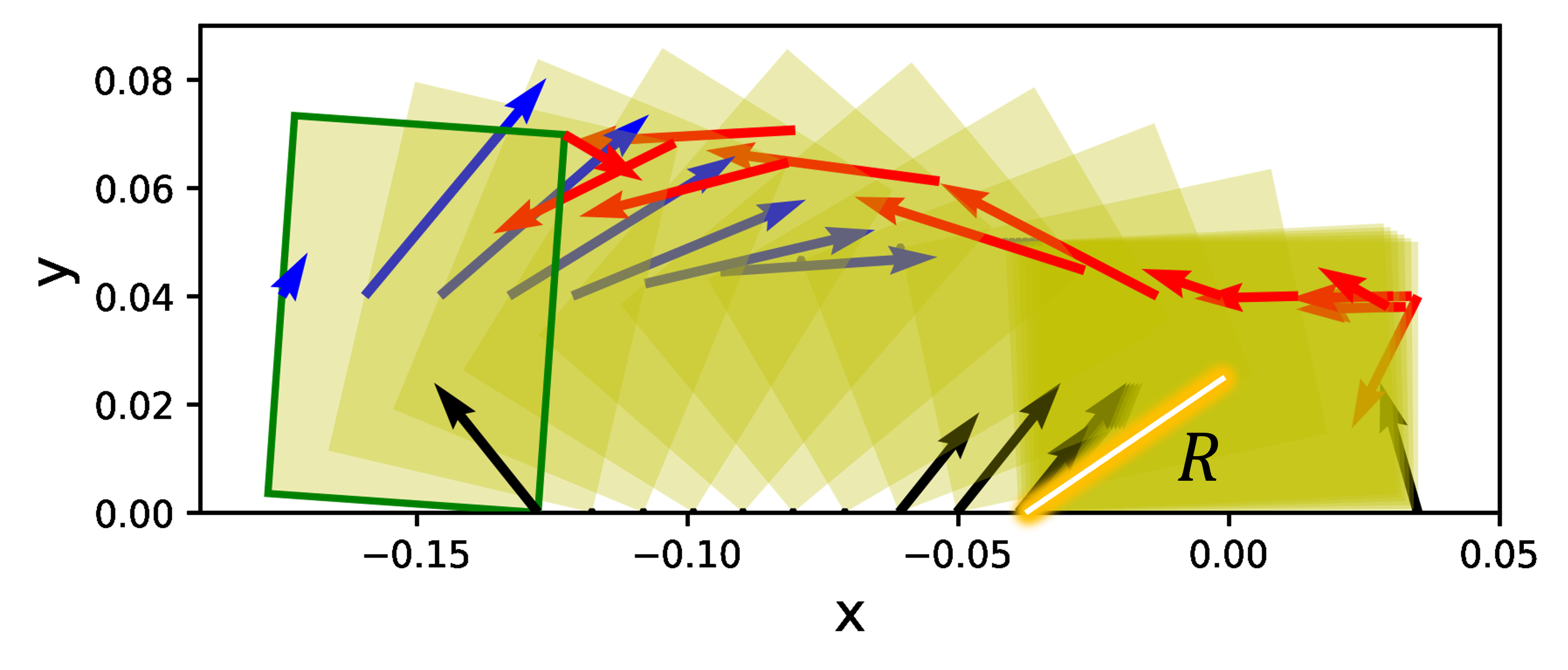
(a) Without robustness cost.

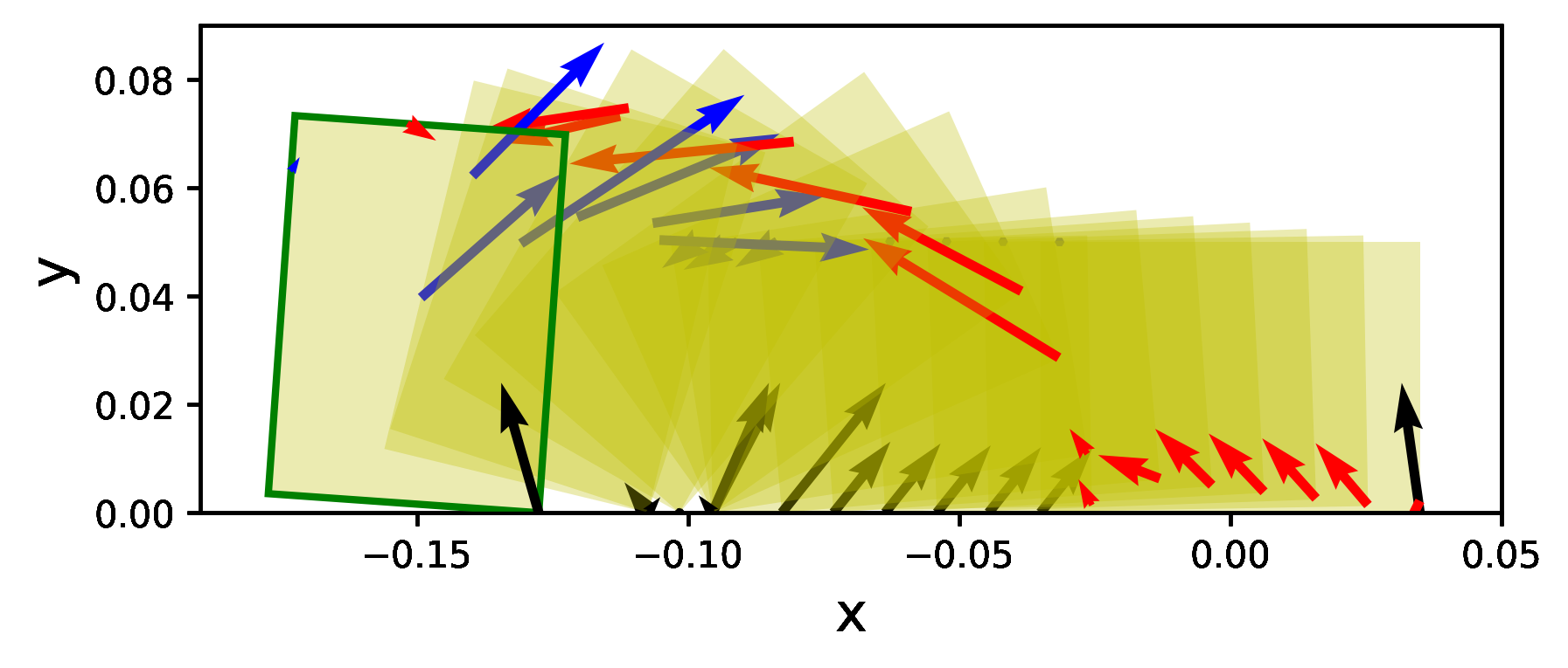
(b) With robustness cost.

Figure 4: Trajectories of pivoting manipulation from Q-Opt. We do not let one of the arms make contact if $q_{y}\geq$-0.05\text{\,}\mathrm{m}$$, denoted as blue arrows. We consider $T=150$ but only plot 15 snapshots with no gravity arrows (aligned along $y$-axis.), for clarity. The bold green line represents the goal state. The orange line shows $R$ at $t=0$ (see Sec V-B).

V-A Experiment Setup

We implement our framework in Python using SNOPT [37] with Drake [38] for solving K-Opt and Q-Opt. We use Gurobi [39] for solving C-Opt. The computation is tested on a computer with Intel i9-13900K. For hardware experiments, we use a Mitsubishi Electric Assista arm with a stiffness controller, equipped with a WSG-32 gripper. The object pose is measured using AprilTag [40].

V-B Results of Generated Trajectories using Our framework

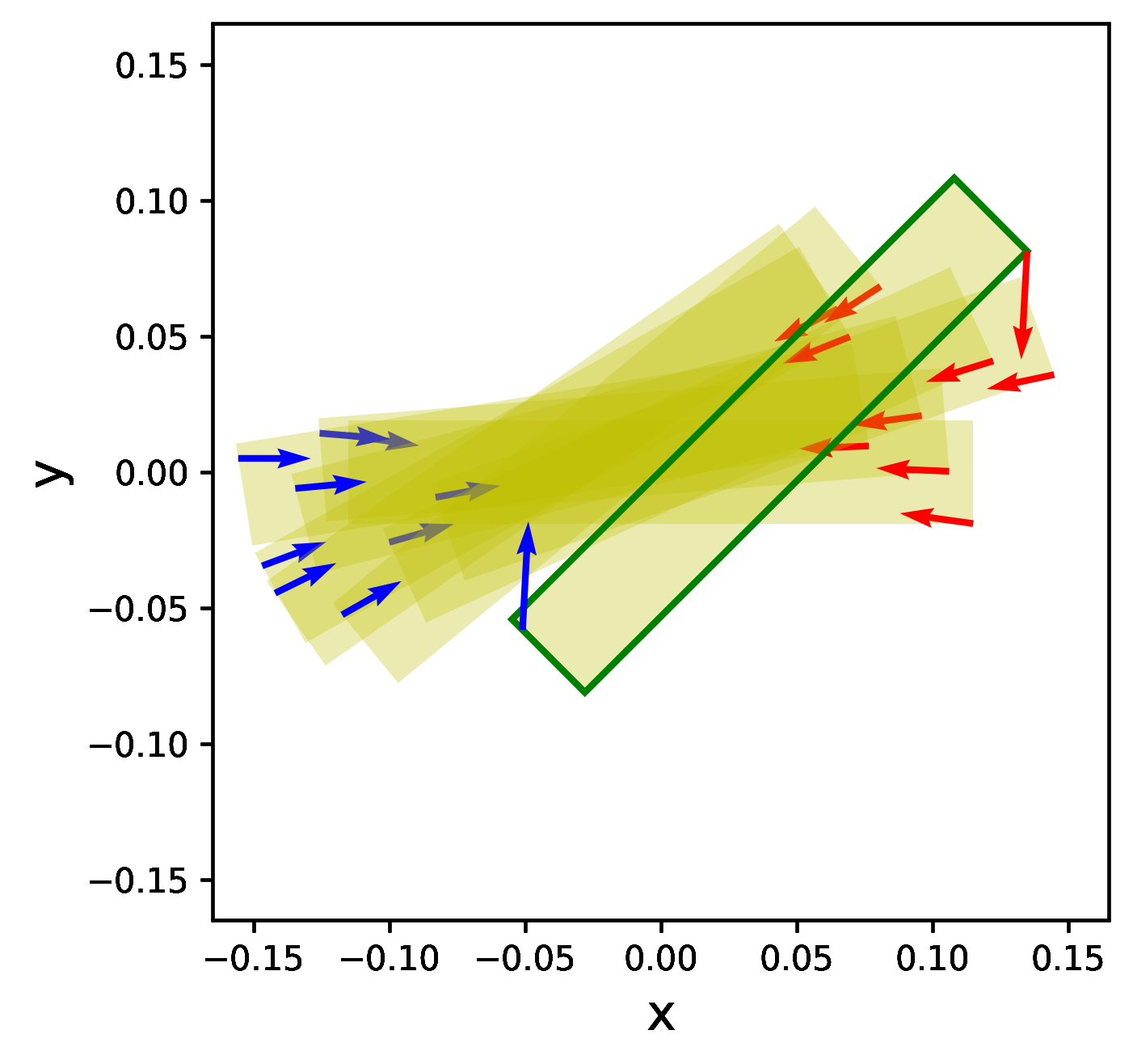
(a) Output of C-Opt.

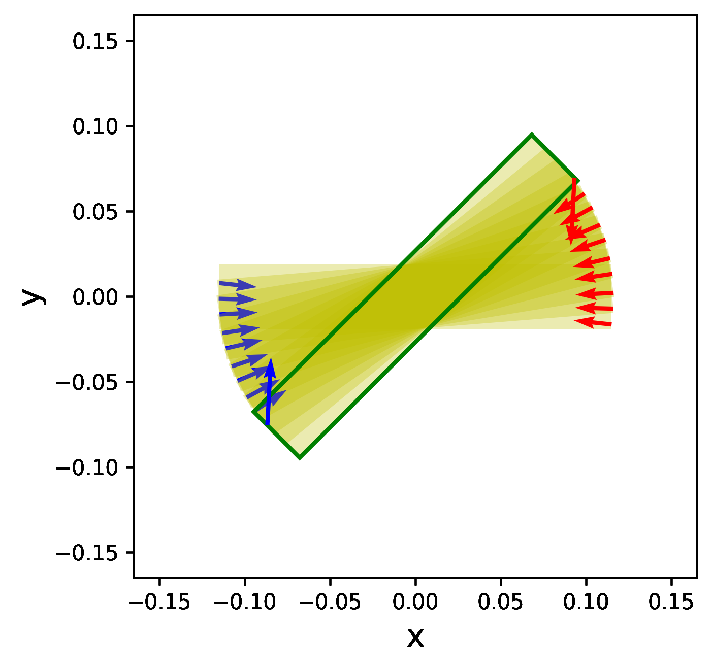
(b) Output of Q-Opt.

Figure 5: Trajectories for sliding manipulation to rotate the object by $45\text{\,}\mathrm{\SIUnitSymbolDegree}$. Because Q-Opt can consider full nonlinear dynamics, it could achieve better motion than C-Opt. Note that we consider $T=50$ but only plot 10 snapshots for clarity. The bold green line represents the goal state.

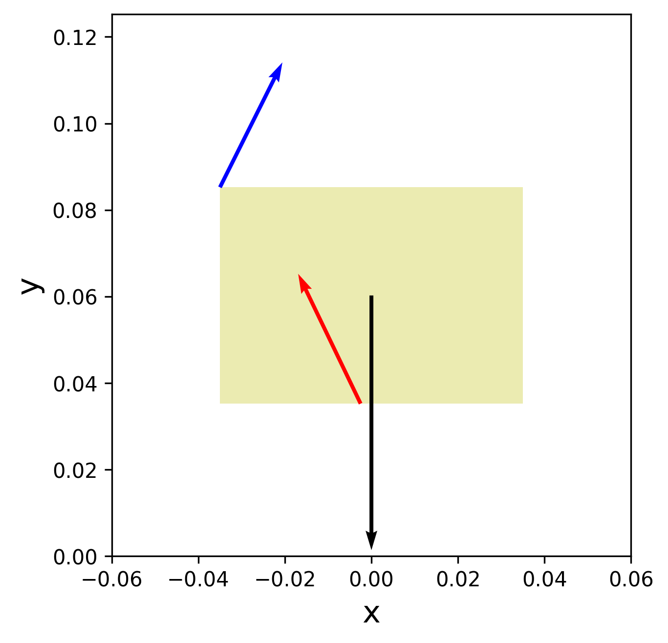
(a)

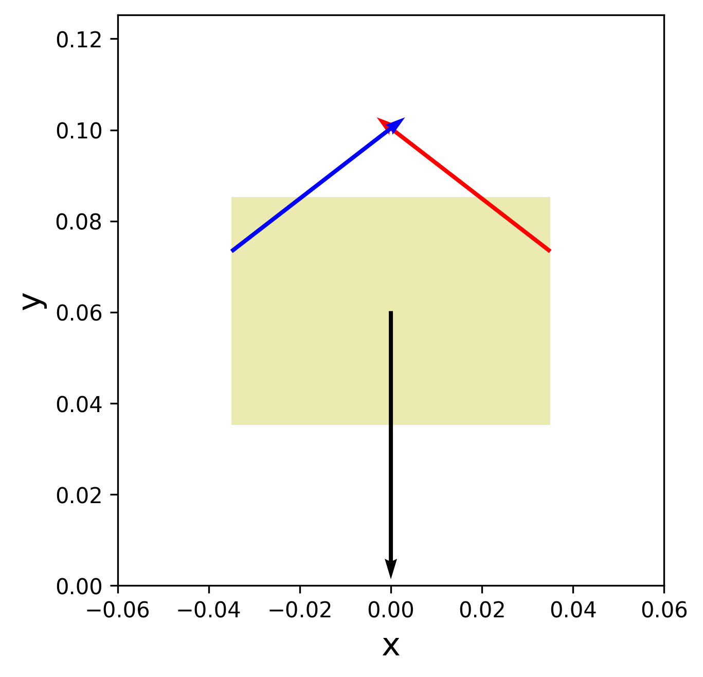
(b)

Figure 6: We show how C-Opt generates robot contact location using (a) McCormick envelope and (b) ours. Black arrow shows gravity.

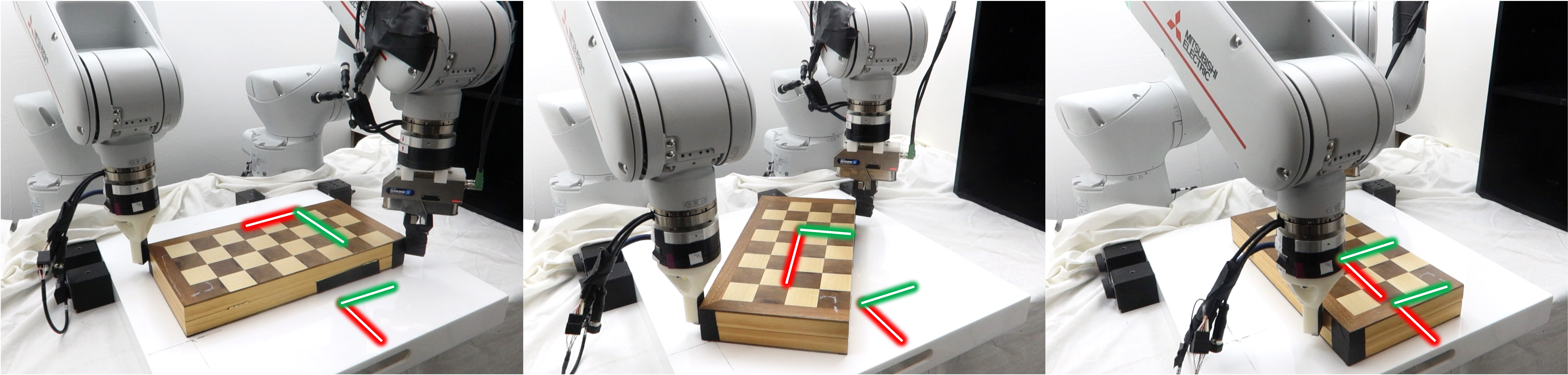
(a) Dual arm sliding

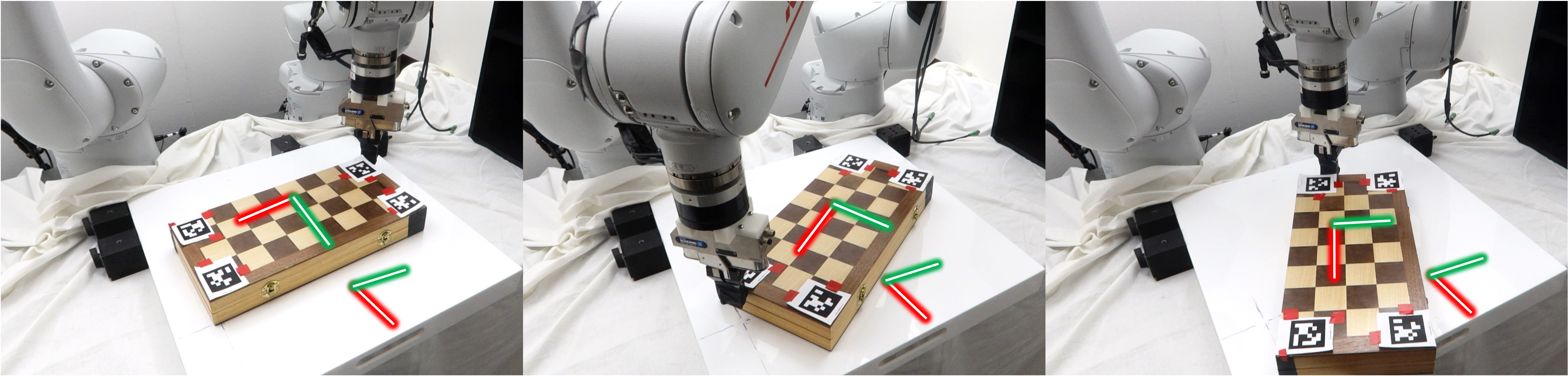
(b) Single arm sliding

Figure 7: Demonstration of sliding manipulation of a box in hardware experiments using the proposed algorithm. In Fig. 7(a), the robots do not change the contact location on the object. In Fig. 7(b), the robot has to change its contact location to accomplish its task. The arrows represent the current orientation of the object and its desired orientation at the terminal time-step. The Apriltag system is used for feedback during the change of the contact location to ensure that the robot makes contact in the correct location. The hardware experiment video is found here.

First, we discuss how our method, C-Opt and Q-Opt, work together to achieve versatile contact-rich trajectories. To discuss this, we consider the pivoting task with one extrinsic contact with the environment. The goal is to rotate the object by $90\text{\,}\mathrm{\SIUnitSymbolDegree}$. We do not allow one of the arms to make contact if $q_{y}\geq$-0.05\text{\,}\mathrm{m}$$, to consider the workspace of the arm. Given the trajectory from C-Opt, we consider two cases. In the 1st case, for each time step $t$, we consider the robustness cost, $\max(R(\cos{q_{\theta_{t}})^{2}})$ in Q-Opt, where $R$ is the distance between the extrinsic contact location and the center of mass of the object (see Fig. 4). In the 2nd case, we omit this cost.

The results are shown in Fig. 4. In Fig. 4(a), the robot keeps pivoting the object until another arm starts supporting the object after $q_{y}\geq$-0.05\text{\,}\mathrm{m}$$. In contrast, in Fig. 4(b), one of the arms first pushes the object around $q_{y}=$-0.05\text{\,}\mathrm{m}$$ and then both arms pivot the object together. This is because using two arms minimizes the time the object remains unstable in gravity, ensuring better stability. Hence, that robust cost is maximized. This is achieved because Q-Opt is capable of updating the trajectory of $\mathbf{q}_{t}$ based on user requirements.

Next, we discuss the scenario where the goal is to slide the object on the table by $45\text{\,}\mathrm{\SIUnitSymbolDegree}$ with no position drifts. The results are shown in Fig. 5. From Fig. 5(a) and Fig. 5(b), Q-Opt could achieve significantly less drift in position than C-Opt. This is because Q-Opt can consider the full nonlinear dynamics, and thus it can utilize the nonlinearity of the system. This highlights that our framework can provide a descent trajectory of the system as long as C-Opt provides decent contact information.

V-C Results of Convex Relaxation of Bilinear Terms

Next, we verify that the proposed convex relaxation of bilinear constraints results in tigher solutions. We consider a grasping task where the goal is to lift the object. We consider C-Opt using McCormick envelope (4) and ours (6) with $K=2$. The results are illustrated in Fig. 6. In Fig. 6(a), it is obvious that there is clock-wise moment exists while in Fig. 6(b), moment balance is satisfied. Thus, our proposed relaxation could achieve a tighter estimation of bilinear terms. We also observe that our method where C-Opt uses (6) shows a higher success rate than our method where C-Opt uses (4) (see Table II) with some cost of computation. This makes sense since Q-Opt has higher chances of finding feasible solutions if C-Opt provides better solutions.

V-D Computational Results

We discuss the computational results. We consider 500 different initial and goal states of the box whose width and height are $0.07\text{\,}\mathrm{m}$ and $0.05\text{\,}\mathrm{m}$, respectively. We sample initial and goal states of the object uniformly from the range of $\pm$0.05\text{\,}\mathrm{m}$$ of $x$- and $y$-positions, and $\pm$90\text{\,}\mathrm{\SIUnitSymbolDegree}$$ of the angle of the object, respectively. For each initial and goal pose of the object, we run optimizers. For all samples, we use $h=0.2$s. All options are summarized in Table II.

Success Rate. We consider $T=200$. We define success as the optimizer finding a feasible solution within 1 minute. We denote $S_{i}$ as the success rate of the $i$-th option and we got $S_{1}=8\%,S_{2}=22\%,S_{3}=41\%,S_{4}=71\%$.

Computation Time. The results are summarized in Table II. Overall, we observe that option 4 (ours) shows the best performance. First, the total computation time in option 4 is generally the smallest among options. Second, option 4 and option 1 show smaller $a_{2}$ (defined in Table II) than other options. This makes sense since for these options, C-Opt converges quickly because of numerical efficiency. Third, we observe that the number of iterations in option 2, to add cutting plane denoted as $a_{3}$, is largest compared to other methods because the naive McCormick envelope does not provide good quality solutions due to relatively rough approximation of bilinear constraints, resulting in many cuts.

V-E Hardware Experiments

We implement the trajectories generated by our framework on a robotic system in open-loop. We consider two tasks, a stowing task where the goal is to stow an object on a shelf, and a sliding task where the goal is to rotate the object by $90\text{\,}\mathrm{\SIUnitSymbolDegree}$. The results are shown in Fig. 1 and Fig. 7. We observe that the robot(s) could successfully achieve the desired tasks in Fig. 1 and Fig. 7(a). Note that Fig. 7(b) shows that the single arm could not complete its task due to open-loop control.

TABLE II: Computation results for different options and time horizons. Each option differs in how C-Opt computes. Option 1 is the baseline where Gurobi solves the original mixed-integer non-convex QCQP (2) in C-Opt. Option 2 uses the naive McCormick envelope (4). Option 3 uses the piecewise McCormick envelope (5) with $C=8$. Option 4 uses our piecewise McCormick envelope using binary encoding (6) with $K=3$. Each entry contains three values: $a_{1},a_{2},a_{3}$. $a_{1}$ is the average total computation time (i.e., runtime of C-Opt + Q-Opt) in second. $a_{2}$ is the average ratio of the computation time spent in C-Opt over $a_{1}$. $a_{3}$ is the average number of cuts (i.e., the number of iterations between C-Opt and Q-Opt). We compute these values over the successful samples defined in Sec. V-D.

Options	Time Horizon ($T$)
	$T=50$	$T=100$	$T=200$
1	(28, 0.80, 1.0)	(56, 0.79, 1.9)	(59, 0.89, 2.1)
2	(0.9, 0.14, 18.5)	(50, 0.11, 25.5)	(59, 0.29, 70.2)
3	(10, 0.53, 7.1)	(44, 0.80, 10.9)	(55, 0.88, 21.9)
4	(6, 0.30, 6.1)	(9, 0.35, 10.1)	(11, 0.55, 20.1)

We discuss the results of the sliding task. In Fig. 7(a), we consider two arms while in Fig. 7(b) we consider a single-arm manipulation. We observe that in Fig. 7(a), the bimanual maintains the same contact location but in Fig. 7(b) the single arm keeps changing the contact location on the object so as to achieve the desired goal. Therefore, our framework can automatically achieve very different manipulation behavior given underlying constraints (in this case, single point contact vs two contacts). These experiments also verify that our algorithm can generate physically meaningful solutions.

VI Discussion

In this paper, we propose a framework for efficiently computing optimal trajectories of an object, robots, and contact simultaneously using hierarchical optimization. We decompose the original problem into C-Opt and Q-Opt to handle multi-modal manipulation tasks efficiently. In particular, we present a convex relaxation of bilinear constraints using the binary encoding method so that C-Opt can provide tighter solutions. We demonstrate and verify our method extensively under various scenarios including hardware experiments.

Future Work. Although our method can realize multi-modal manipulation, our method may fail if the trajectory by K-Opt does not satisfy system dynamics. Thus, the key question we want to answer is how we obtain a kinematics trajectory in K-Opt that has a high chance of satisfying the system dynamics. Ultimately, we want to understand how to update the kinematics trajectory when the proposed method fails to find a feasible solution based on the infeasible solution. Similarly, we are interested in working on adding more informative cuts to C-Opt if Q-Opt only finds infeasible solutions. Our current cutting-plane method does not fully utilize the infeasible solution by Q-Opt so it is interesting how to encode informative information to add better cuts. Lastly, this paper focuses on contact at the robot’s end-effector, but we aim to extend our approach to whole-body robot contacts (e.g., [41, 17, 18, 42]) for more generalized multi-modal manipulation.

References

- [1] K. Ota, D. K. Jha, S. Jain, B. Yerazunis, R. Corcodel, Y. Shukla, A. Bronars, and D. Romeres, “Autonomous robotic assembly: From part singulation to precise assembly,” in 2024 IEEE/RSJ International Conference on Intelligent Robots and Systems (IROS), 2024, pp. 13 525–13 532.
- [2] A. Billard and D. Kragic, “Trends and challenges in robot manipulation,” Science, vol. 364, no. 6446, p. eaat8414, 2019.
- [3] S. Saha and A. A. Julius, “Task and motion planning for manipulator arms with metric temporal logic specifications,” IEEE robotics and automation letters, vol. 3, no. 1, pp. 379–386, 2017.
- [4] Z. Zhao, Z. Zhou, M. Park, and Y. Zhao, “Sydebo: Symbolic-decision-embedded bilevel optimization for long-horizon manipulation in dynamic environments,” IEEE Access, vol. 9, pp. 128 817–128 826, 2021.
- [5] M. Toussaint, J. Harris, J.-S. Ha, D. Driess, and W. Hönig, “Sequence-of-constraints mpc: Reactive timing-optimal control of sequential manipulation,” in 2022 IEEE/RSJ International Conference on Intelligent Robots and Systems (IROS). IEEE, 2022, pp. 13 753–13 760.
- [6] T. Stouraitis, I. Chatzinikolaidis, M. Gienger, and S. Vijayakumar, “Online hybrid motion planning for dyadic collaborative manipulation via bilevel optimization,” IEEE Transactions on Robotics, vol. 36, no. 5, pp. 1452–1471, 2020.
- [7] M. Posa, C. Cantu, and R. Tedrake, “A direct method for trajectory optimization of rigid bodies through contact,” Int. J. Rob. Res., vol. 33, no. 1, pp. 69–81, 2014.
- [8] A. Patel, S. L. Shield, S. Kazi, A. M. Johnson, and L. T. Biegler, “Contact-implicit trajectory optimization using orthogonal collocation,” IEEE Robotics and Automation Letters, vol. 4, no. 2, pp. 2242–2249, 2019.
- [9] J. Moura, T. Stouraitis, and S. Vijayakumar, “Non-prehensile planar manipulation via trajectory optimization with complementarity constraints,” in 2022 International Conference on Robotics and Automation (ICRA). IEEE, 2022, pp. 970–976.
- [10] M. Zhang, D. K. Jha, A. U. Raghunathan, and K. Hauser, “Simultaneous trajectory optimization and contact selection for multi-modal manipulation planning,” arXiv preprint arXiv:2306.06465, 2023.
- [11] Y. Shirai, D. K. Jha, and A. U. Raghunathan, “Covariance steering for uncertain contact-rich systems,” in 2023 IEEE International Conference on Robotics and Automation (ICRA). IEEE, 2023, pp. 7923–7929.
- [12] A. K. Valenzuela, “Mixed-integer convex optimization for planning aggressive motions of legged robots over rough terrain,” Ph.D. dissertation, Massachusetts Institute of Technology, 2016.
- [13] B. Aceituno-Cabezas, C. Mastalli, H. Dai, M. Focchi, A. Radulescu, D. G. Caldwell, J. Cappelletto, J. C. Grieco, G. Fernández-López, and C. Semini, “Simultaneous contact, gait, and motion planning for robust multilegged locomotion via mixed-integer convex optimization,” IEEE Robotics and Automation Letters, vol. 3, no. 3, pp. 2531–2538, 2017.
- [14] B. Aceituno-Cabezas and A. Rodriguez, “A global quasi-dynamic model for contact-trajectory optimization in manipulation,” in Robotics: Science and Systems Foundation, 2020.
- [15] Y. Ding, C. Li, and H.-W. Park, “Kinodynamic motion planning for multi-legged robot jumping via mixed-integer convex program,” in 2020 IEEE/RSJ International Conference on Intelligent Robots and Systems (IROS). IEEE, 2020, pp. 3998–4005.
- [16] Y. Shirai, X. Lin, A. Schperberg, Y. Tanaka, H. Kato, V. Vichathorn, and D. Hong, “Simultaneous contact-rich grasping and locomotion via distributed optimization enabling free-climbing for multi-limbed robots,” in Proc. 2022 IEEE/RSJ Int. Conf. Intell. Rob. Syst., 2022, pp. 13 563–13 570.
- [17] T. Pang, H. T. Suh, L. Yang, and R. Tedrake, “Global planning for contact-rich manipulation via local smoothing of quasi-dynamic contact models,” IEEE Transactions on robotics, 2023.
- [18] Y. Shirai, T. Zhao, H. Suh, H. Zhu, X. Ni, J. Wang, M. Simchowitz, and T. Pang, “Is linear feedback on smoothed dynamics sufficient for stabilizing contact-rich plans?” 2025 International Conference on Robotics and Automation (ICRA), 2025.
- [19] B. P. Graesdal, S. Y. C. Chia, T. Marcucci, S. Morozov, A. Amice, P. A. Parrilo, and R. Tedrake, “Towards tight convex relaxations for contact-rich manipulation,” in Proceedings of Robotics: Science and Systems (RSS), 2024.
- [20] G. P. McCormick, “Computability of global solutions to factorable nonconvex programs: Part i—convex underestimating problems,” Mathematical programming, vol. 10, no. 1, pp. 147–175, 1976.
- [21] B. Ponton, A. Herzog, S. Schaal, and L. Righetti, “A convex model of humanoid momentum dynamics for multi-contact motion generation,” in 2016 IEEE-RAS 16th International Conference on Humanoid Robots (Humanoids). IEEE, 2016, pp. 842–849.
- [22] B. Ponton, M. Khadiv, A. Meduri, and L. Righetti, “Efficient multicontact pattern generation with sequential convex approximations of the centroidal dynamics,” IEEE Transactions on Robotics, vol. 37, no. 5, pp. 1661–1679, 2021.
- [23] X. Lin, M. S. Ahn, and D. Hong, “Designing multi-stage coupled convex programming with data-driven mccormick envelope relaxations for motion planning,” in 2021 IEEE International Conference on Robotics and Automation (ICRA). IEEE, 2021, pp. 9957–9963.
- [24] J. P. Vielma and G. L. Nemhauser, “Modeling disjunctive constraints with a logarithmic number of binary variables and constraints,” Mathematical Programming, vol. 128, pp. 49–72, 2011.
- [25] N. Chavan-Dafle, R. Holladay, and A. Rodriguez, “In-hand manipulation via motion cones,” arXiv preprint arXiv:1810.00219, 2018.
- [26] Y. Shirai, D. K. Jha, A. U. Raghunathan, and D. Hong, “Tactile tool manipulation,” in 2023 IEEE International Conference on Robotics and Automation (ICRA). IEEE, 2023, pp. 12 597–12 603.
- [27] O. Taylor, N. Doshi, and A. Rodriguez, “Object manipulation through contact configuration regulation: multiple and intermittent contacts,” in 2023 IEEE/RSJ International Conference on Intelligent Robots and Systems (IROS). IEEE, 2023, pp. 8735–8743.
- [28] Y. Shirai, D. K. Jha, and A. U. Raghunathan, “Robust pivoting manipulation using contact implicit bilevel optimization,” IEEE Transactions on Robotics, 2024.
- [29] E. Balas, “Disjunctive programming,” Annals of discrete mathematics, vol. 5, pp. 3–51, 1979.
- [30] L. Wang, Y. Xiang, and D. Fox, “Manipulation trajectory optimization with online grasp synthesis and selection,” arXiv preprint arXiv:1911.10280, 2019.
- [31] J.-P. Sleiman, F. Farshidian, and M. Hutter, “Versatile multicontact planning and control for legged loco-manipulation,” Science Robotics, vol. 8, no. 81, p. eadg5014, 2023.
- [32] A. Rigo, M. Hu, S. K. Gupta, and Q. Nguyen, “Hierarchical optimization-based control for whole-body loco-manipulation of heavy objects,” in 2024 IEEE International Conference on Robotics and Automation (ICRA). IEEE, 2024, pp. 15 322–15 328.
- [33] X. Lin, “Accelerate hybrid model predictive control using generalized benders decomposition,” arXiv preprint arXiv:2406.00780, 2024.
- [34] J. Pan, Z. Chen, and P. Abbeel, “Predicting initialization effectiveness for trajectory optimization,” in 2014 IEEE International Conference on Robotics and Automation (ICRA). IEEE, 2014, pp. 5183–5190.
- [35] Y. Hou, Z. Jia, and M. T. Mason, “Manipulation with shared grasping,” arXiv preprint arXiv:2006.02996, 2020.
- [36] Y. Shirai, D. K. Jha, A. U. Raghunathan, and D. Romeres, “Robust pivoting: Exploiting frictional stability using bilevel optimization,” in 2022 International Conference on Robotics and Automation (ICRA). IEEE, 2022, pp. 992–998.
- [37] P. E. Gill, W. Murray, and M. A. Saunders, “Snopt: An sqp algorithm for large-scale constrained optimization,” SIAM review, vol. 47, no. 1, pp. 99–131, 2005.
- [38] R. Tedrake and the Drake Development Team, “Drake: Model-based design and verification for robotics,” 2019. [Online]. Available: https://drake.mit.edu
- [39] Gurobi Optimization, LLC, “Gurobi Optimizer Reference Manual,” 2024. [Online]. Available: https://www.gurobi.com
- [40] J. Wang and E. Olson, “Apriltag 2: Efficient and robust fiducial detection,” in 2016 IEEE/RSJ International Conference on Intelligent Robots and Systems (IROS). IEEE, 2016, pp. 4193–4198.
- [41] M. Murooka, S. Nozawa, Y. Kakiuchi, K. Okada, and M. Inaba, “Whole-body pushing manipulation with contact posture planning of large and heavy object for humanoid robot,” in 2015 IEEE International Conference on Robotics and Automation (ICRA). IEEE, 2015, pp. 5682–5689.
- [42] V. Leve, J. Moura, N. Saito, S. Tonneau, and S. Vijayakumar, “Explicit contact optimization in whole-body contact-rich manipulation,” arXiv preprint arXiv:2408.15726, 2024.