MFC 5.0: An exascale many-physics flow solver

Abstract

Many problems of interest in engineering, medicine, and the fundamental sciences rely on high-fidelity flow simulation, making performant computational fluid dynamics solvers a mainstay of the open-source software community. A previous work (Bryngelson et al.  Comp. Phys. Comm. (2021)) made MFC 3.0 a published, documented, and open-source source solver with numerous physical features, numerical methods, and scalable infrastructure. MFC 5.0 is a marked update to MFC 3.0, including a broad set of well-established and novel physical models and numerical methods and the introduction of GPU and APU (or superchip) acceleration. We exhibit state-of-the-art performance and ideal scaling on the first two exascale supercomputers, OLCF Frontier and LLNL El Capitan. Combined with MFC’s single-accelerator performance, MFC achieves exascale computation in practice. New physical features include the immersed boundary method, $N$-fluid phase change, Euler–Euler and Euler–Lagrange sub-grid bubble models, fluid-structure interaction, hypo- and hyper-elastic materials, chemically reacting flow, two-material surface tension, and more. Numerical techniques now represent the current state-of-the-art, including general relaxation characteristic boundary conditions, WENO variants, Strang splitting for stiff sub-grid flow features, and low Mach number treatments. Weak scaling to tens of thousands of GPUs on OLCF Summit and Frontier and LLNL El Capitan see efficiencies within 5% of ideal to over 90% of their respective system sizes. Strong scaling results for a 16-times increase in device count see parallel efficiencies over 90% on OLCF Frontier. MFC’s software stack has further improved, including continuous integration, which ensures code resilience and correctness through over 300 regression tests; metaprogramming, which reduces code length and maintains performance portability; and code generation for computing chemical reactions.

1 Introduction

MFC was introduced to the literature and open source community via Bryngelson et al. [1]. This work described the software design and features of MFC 3.0, a CPU-based compressible multi-component flow code (MFC) for the 5-equation diffuse interface methods of Kapila et al. [2] and Allaire et al. [3] and the six equation diffuse interface model of Saurel et al. [4]. MFC 3.0 included other features that are discussed throughout this manuscript. Since MFC 3.0’s release, the MFC community has added a broad set of physical models, numerical methods, GPU offloading capabilities, and performance optimizations. This paper focuses holistically on MFC’s development over the past four years. We present physical models, numerical methods, validity, software robustness and testing, and performance on diverse architecture sets at scale on exascale machines and beyond.

1.1 The history of MFC

The MFC codebase archaeology starts in the mid-2000s. At this time, MFC was unnamed solver developed by Eric Johnsen. This code represented multi-component flow with the diffuse interface method, which were described in Johnsen [5] and Johnsen and Colonius [6]. Following this effort, Vedran Coralic performed a major code rewrite and adorned MFC with its name. These features adorned MFC with a multi-dimensional numerical reconstruction treatment and are described in Coralic and Colonius [7]. Jomela Meng added cylindrical coordinates systems and corresponding simulations of high-speed shock–droplet interaction [8]. Kazuki Maeda added an Euler–Lagrange representation of sub-grid bubble dynamics [9] and acoustic wave generation [10]. Kevin Schmidmayer and Spencer Bryngelson added the 5-equation model of Kapila et al. [2] and the 6-equation model of Saurel et al. [4]. These efforts were conducted in the research group of Tim Colonius at the California Institute of Technology. Spencer Bryngelson later led a restructuring of MFC at the Georgia Institute of Technology, including additional modeling and numerics features. This effort culminated in the open-sourcing of MFC 3.0 in 2020 and is largely described in Bryngelson et al. [1]. Modeling, method, and software scalability and portability capabilities were added in subsequent years, which are discussed in this manuscript.

1.2 New MFC capabilities

MFC now includes more capable physical models and numerical methods, software resistance through continuous integration and deployment, code coverage testing, and computation acceleration via GPU and APU devices. Physical features include six new models for phase change, non-polytropic sub-grid bubble dynamics, treatment for elastic materials, chemical reactions and combustion, and surface tension. An immersed boundary method that supports complex geometries from analytical level sets or STL files. New numerical methods include generalized characteristic boundary conditions, improved shock capturing with TENO and WENO-Z constructions, Strang splitting for stiff sub-grid dynamics, and treatment for low-Mach number flow. Significant software additions have made MFC a portable and performant solver on CPUs, GPUs, and APUs from various vendors, including Intel, AMD, and NVIDIA. Significant decreases in run time are in part enabled via metaprogramming and static code generation.

1.3 Use of MFC

MFC has a history of being used for early access programs on flagship supercomputers. At the time of writing, these programs include JSC JUPITER (JUREAP) and the LLNL El Capitan and OLCF Frontier final and early access systems, including LLNL Tioga (AMD MI300A testbed) and OLCF Spock and Crusher (AMD MI100 and MI250X testbeds). Commodity cluster use of MFC is broad, including the ACCESS-CI [11] (formerly XSEDE [12]) clusters (PSC Bridges [13] and Bridges2 [14], SDSC Comet [15] and Expanse [16], Purdue Anvil [17], NCSA Delta [18] and DeltaAI [19], TACC Stampede1–3 [20, 21, 22], among others) university clusters, cloud computer systems (Intel’s AI cloud [23]), and AMD and Cray’s internal systems, among numerous others. MFC is a SPEChpc benchmark candidate, which comprises software that evaluates the performance of supercomputers [24].

1.4 Manuscript structure

In section 2, we introduce MFC 5.0, describing the code and methods it builds upon while connecting it to MFC 3.0. Section 3 discusses established numerical methods that MFC builds upon. New features follow in section 4, including physical models, numerical methods, and software tooling. We show exemplar MFC simulations in section 5. A discuss other open source flow solvers with some similar features in section 6. Section 7 summarizes the manuscript and MFC 5.0.

2 Multiphase models

2.1 Multi-component treatment

MFC uses reduced versions of the Baer–Nunziato model [25] and diffuse interface methods to model multiphase flow. Diffuse interface methods model the presence of each species using volume fractions and allow for a small region of smearing between species. Other approaches to multiphase flow modeling require interface tracking, which requires coupled flow solvers and complex mesh management [26]. Alternatively, mesh-free methods like smoothed particle hydrodynamics could be used but smoothed particle hydrodynamics requires extensive load balancing and careful treatment of boundary conditions [26]. Diffuse interface methods are used to avoid these difficulties.

2.1.1 Five-equation models

For a two-fluid flow configuration, the Baer–Nunziato model reduces to the so-called five-equation model

$$\frac{\partial\alpha_{i}\rho_{i}}{\partial t}+\nabla\cdot(\alpha_{i}\rho_{i}\bm{u}) =0,$$

$$\frac{\partial\rho\bm{u}}{\partial t}+\nabla\cdot(\bm{u}\otimes\bm{u}+p\bm{I}-\bm{T}^{v}) =0,$$

$$\frac{\partial\rho E}{\partial t}+\nabla\cdot\left[(\rho E+p)\bm{u}-\bm{T}^{v}\cdot\bm{u}\right] =0,$$

$$\frac{\partial\alpha_{i}}{\partial t}+\bm{u}\cdot\nabla\alpha_{i} =K\nabla\cdot\bm{u},$$

of Kapila et al. [2] by assuming that both species share a velocity and pressure, and $i=1,\dots,N_{\mathrm{comp.}}$ where $N_{\mathrm{comp.}}$ is the number of fluid components. With this model, $\rho$, $\bm{u}$, $p$, and $E$ are the mixture density, velocity, pressure, and total energy (per unit mass). The $\alpha_{i}$ and $\rho_{i}$ are the volume fraction and density of component $i$. Viscous terms are introduced via the mixture viscous stress tensor

$$\bm{T}^{v}=2\eta(\bm{D}-\operatorname{tr}(\bm{D})\bm{I}/3),$$ (1)

where $\eta$ is the mixture shear viscosity and the strain rate tensor is

$$\bm{D}=(\nabla\bm{u}+(\nabla\bm{u})^{\top})/2.$$ (2)

The mixture internal energy $e$ is

$$e=Y_{1}e(\rho_{1}p)+Y_{2}e(\rho_{2}p),$$ (3)

where $Y_{i}=\alpha_{i}\rho_{i}/\rho$ is the mass fraction of component $i$. The model is closed using the mixture rules

$$1=\sum_{i=1}^{N}\alpha_{i},\quad\rho=\sum_{i=1}^{N}\alpha_{i}\rho_{i},\quad\rho e=\sum_{i=1}^{N}\alpha_{i}\rho_{i}e_{i}.$$ (4)

For two components, $K$ is

$$K=\frac{\rho_{2}c_{2}^{2}+\rho_{1}c_{1}^{2}}{\rho_{1}c_{1}^{2}/\alpha_{1}+\rho_{2}c_{2}^{2}/\alpha_{2}},$$ (5)

where $c_{i}$ is phasic sound speed

$$c_{i}=\sqrt{\gamma_{i}(p+\pi_{\infty,i})/\rho_{i}}.$$ (6)

The term $K\nabla\cdot\bm{u}$ ensures thermodynamic consistency and accounts for the expansion and compression of each species in mixture regions. The $K\nabla\cdot\bm{u}$ is necessary to model phenomena like spherical bubble collapse [27], but it is non-conservative and can lead to numerical instabilities [27]. For some problems, $K\nabla\cdot\bm{u}$ is not necessary, and the model reduces to that of Allaire et al. [3]. Differences between these models are discussed in Schmidmayer et al. [27].

2.1.2 Six-equation model

The six-equation model of Saurel et al. [4] allows for pressure disequilibrium between phases and can be used to avoid numerical stability issues associated with the five-equation Kapila model, while maintaining thermodynamic consistency. For two fluids, the six-equation model is

$$\frac{\partial\alpha_{i}\rho_{i}}{\partial t}+\nabla\cdot(\alpha_{i}\rho_{i}\bm{u}) =0,$$

$$\frac{\partial\rho\bm{u}}{\partial t}+\nabla\cdot(\rho\bm{u}\bm{u}+p\bm{I}-\bm{T}^{v}) =0.$$

$$\frac{\partial\alpha_{1}\rho_{1}e_{1}}{\partial t}+\nabla\cdot(\alpha_{1}\rho_{1}e_{1}\bm{u})+\alpha_{1}p_{1}\cdot\nabla\bm{u} =-\mu p_{\mathrm{I}}(p_{2}-p_{1})-\alpha_{1}\bm{T}_{1}^{v}:\nabla\bm{u},$$

$$\frac{\partial\alpha_{2}\rho_{2}e_{2}}{\partial t}+\nabla\cdot(\alpha_{1}\rho_{2}e_{2}\bm{u})+\alpha_{2}p_{2}\cdot\nabla\bm{u} =-\mu p_{\mathrm{I}}(p_{1}-p_{2})-\alpha_{2}\bm{T}_{2}^{v}:\nabla\bm{u},$$

$$\frac{\partial\alpha_{1}}{\partial t}+\bm{u}\cdot\nabla\alpha_{1} =\mu(p_{1}-p_{2}).$$

Here, $\rho$ and $\bm{u}$ are the mixture density and velocity, $\alpha_{i}$, $\rho_{i}$, $p_{i}$, $e_{i}$, and $\bm{T}_{i}^{v}$ are the volume fraction, density, pressure, internal energy, and species viscous stress tensor of species $i$ and $\mu$ is a pressure relaxation parameter. The interfacial pressure $P_{\mathrm{I}}$ is

$$P_{\mathrm{I}}=\frac{z_{2}p_{1}+z_{1}p_{2}}{z_{1}+z_{2}},$$ (7)

where $z_{i}=\rho_{i}c_{i}$ is the phasic acoustic impedance and the phasic speed of sound $c_{i}$ is

$$c_{i}=\sqrt{\gamma(p_{i}+\pi_{\infty,i})/\rho_{i}}.$$ (8)

The model is closed using the same mixture rules of the five-equation model in section 2.1.1. Following Schmidmayer et al. [27], the six-equation model in the limit of infinite relaxation can represent the same physical processes as the model of Kapila et al. [2], but avoids numerical instability issues that arise from some interface capture schemes.

2.2 Equation of state

The five- and six-equation models are closed using the stiffened gas equation of state (EOS), which faithfully models liquids and gasses [28]. In its simplest form, the stiffened gas EOS relates the internal energy to the pressure and density of each species $i$ as

$$e_{i}=\frac{p_{i}+\gamma_{i}\pi_{\infty,i}}{(\gamma_{i}-1)\rho_{i}},$$

where $e_{i}$, $p_{i}$, and $\rho_{i}$ are the internal energy, pressure, and density of species $i$. Parameter $\gamma_{i}$ and the liquid stiffness $\pi_{\infty,i}$ can be tuned to represent different liquids and gases.

2.3 Cylindrical coordinates

Axisymmetric and cylindrical coordinates are implemented via the strategies of Johnsen [5] and Meng [8]. The singularity at $r\to 0$ is handled by placing the axis at a cell boundary such that the radius is defined at the cell center. Then, the solution in cells 180 degrees from each other to support stencils for reconstruction. Spectral filtering in the azimuthal direction relaxes the strict time-step restrictions induced by the small cells near the axis [29].

3 Numerical methods

We next describe the method used to solve for the advective and diffusive terms in the multi-component models of MFC. The strategy closely follows that of Bryngelson et al. [1].

3.1 Finite volume method

The models in MFC are solved using a finite volume method based on the framework of Coralic and Colonius [7]. The model equations take the form

$$\frac{\partial\bm{q}}{\partial t}+\frac{\partial\bm{F}^{(x)}(\bm{q})}{\partial x}+\frac{\partial\bm{F}^{(y)}(\bm{q})}{\partial y}+\frac{\partial\bm{F}^{(z)}(\bm{q})}{\partial z}=\bm{s}(\bm{q})-\bm{h}(\bm{q})\nabla\cdot\bm{u},$$ (9)

where $\bm{q}$ is the vector of cell-averaged conservative variables, $\bm{s}$ and $\bm{h}(\bm{q})$ are source terms, and $\bm{F}^{x},\ \bm{F}^{y},$ and $\bm{F}^{z}$ are the fluxes in the $x$-, $y$- and $z$-directions. 9 is integrated in space across each cell-center as

$$\frac{\partial\bm{q}_{i,j,k}}{\partial t}=\frac{1}{\Delta x_{i}} \left(\bm{F}^{(x)}_{i-1/2,j,k}-\bm{F}^{(x)}_{i+1/2,j,k}\right)+\frac{1}{\Delta y_{j}}\left(\bm{F}^{(y)}_{i,j-1/2,k}-\bm{F}^{(y)}_{i,j+1/2,k}\right)+...$$ (10)

$$\frac{1}{\Delta z_{k}}\left(\bm{F}^{(z)}_{i,j,k-1/2}-\bm{F}^{(z)}_{i,j,k+1/2}\right)+\bm{s}(q_{i,j,k})-\bm{h}(\bm{q}_{i,j,k})\left(\nabla\cdot\bm{u}\right)_{i,j,k}$$

The flux $\bm{F}^{x}(\bm{q}_{i+1/2,j,k})$ is calculated at the center of the face $\bm{A}_{i+1/2,j,k}$ with all other fluxes being calculated similarly. The divergence term is calculated as

$$\begin{aligned} \left(\nabla\cdot\bm{u}\right)_{i,j,k}=\frac{1}{\Delta x_{i}}&\left(u^{(x)}_{i+1/2,j,k}-u^{(x)}_{i-1/2,j,k}\right)+\frac{1}{\Delta y_{j}}\left(u^{(y)}_{i,j+1/2,k}-u^{(y)}_{i,j-1/2,k}\right)+\\ \frac{1}{\Delta z_{k}}&\left(u^{(z)}_{i,j,k+1/2}-u^{(z)}_{i,j,k-1/2}\right)\end{aligned}.$$

3.2 Shock and interface capturing

3.2.1 WENO Reconstructions

The fluxes in finite-volume methods are calculated using the left and right state of each interface by solving the Riemann problem

$$\bm{F}^{(x)}_{i+1/2,j,k} =\bm{F}^{(x)}\left(\bm{q}^{\mathrm{(L)}}_{i+1/2,j,k},\bm{q}^{\mathrm{(R)}}_{i+1/2,j,k}\right),$$

$$\bm{u}^{(x)}_{i+1/2,j,k} =\bm{u}^{(x)}\left(\bm{q}^{\mathrm{(L)}}_{i+1/2,j,k},\bm{q}^{\mathrm{(R)}}_{i+1/2,j,k}\right),$$

where superscripts $\mathrm{(L)}$ and $\mathrm{(R)}$ indicate the state variables reconstructed from the left- and right-hand sides of the finite volume interface. The simplest reconstruction assumes that the state variables are piecewise constant in each cell. This assumption gives the reconstruction

$$\bm{q}^{\mathrm{(L)}}_{i+1/2,j,k}=\bm{q}_{i,j,k}\quad\text{and}\quad\bm{q}^{\mathrm{(R)}}_{i+1/2,j,k}=\bm{q}_{i+1,j,k}.$$

The piecewise constant assumption results in a first-order total variation diminishing (TVD) scheme that obviates oscillations at interfaces but is low-order accurate, resulting in meaningful numerical dissipation. High-order shock- and interface-capturing weighted essentially non-oscillatory (WENO) reconstructions prevent the smearing of continuities and allow for the capture of strong shockwaves and material interfaces.

WENO reconstructions obtain high-order spatial accuracy by considering a convex combination of lower-order reconstructions. A $(2k-1)$-th order WENO reconstruction in the $x$-direction uses $k$ staggered candidate polynomials to reconstruct the state variable $f_{i+1/2,j,k}$ with $f^{\mathrm{(r)}}_{i+1/2,j,k}$ for $r=0,1,\dots,k-1$. The weighted sum of candidate polynomials,

$$f_{i+1/2,j,k}=\sum_{r=0}^{k-1}\omega_{r}f^{\mathrm{(r)}}_{i+1/2,j,k},$$

gives the reconstructed state variable $f_{i+1/2,j,k}$. The nonlinear weights $\omega_{r}$ are calculated via the ideal weights $d_{r}$ and smoothness indicators $\beta_{r}$. The reconstruction of $f_{i,j+1/2,k}$ and $f_{i,j,k+1}$ in the $y$- and $z$-directions are calculated using the same procedure. Fifth-order accuracy is maintained via mapped weights, following Henrick et al. [30]. WENO reconstructions can cause spurious oscillations near material interfaces because they are not TVD for such advection equations. Spurious oscillations are avoided by reconstructing the primitive variables, $\{\alpha\rho_{i},\bm{u},p,\alpha_{i}\}$, intead of the conservatives ones $\{\alpha\rho_{i},\rho\bm{u},E,\alpha_{i}\}$ where $i$ is enumerated over the number of components.

3.2.2 Approximate Riemann solver

The Riemann problem at each finite volume interface is solved using either the Harten–Lax–van Leer (HLL) or the Harten–Lax-van Leer contact (HLLC) approximate Riemann solver [31]. The HLL approximate Riemann solver admits three constant states separated by two discontinuities with wave speeds $S_{\mathrm{L}}$ and $S_{\mathrm{R}}$. The state at the interface between cells $i$ and $i+1$ is

$$\bm{q}_{i+1/2,j,k}=\begin{cases}\bm{q}^{\mathrm{(L)}}_{i+1/2,j,k}&S_{\mathrm{L}}\geq 0,\\ \bm{q}^{\mathrm{(HLL)}}&S_{\mathrm{L}}\leq 0\leq S_{\mathrm{R}},\\ \bm{q}^{\mathrm{(R)}}_{i+1/2,j,k}&0\geq S_{\mathrm{R}},\end{cases}$$

where the constant start state is

$$\bm{q}^{\mathrm{(HLL)}}=\frac{S_{\mathrm{R}}\bm{q}^{\mathrm{(R)}}_{i+1/2,j,k}-S_{\mathrm{L}}\bm{q}^{\mathrm{(L)}}_{i+1/2,j,k}+\bm{F}(\bm{q}^{\mathrm{(L)}}_{i+1/2,j,k})-\bm{F}(\bm{q}^{\mathrm{(R)}}_{i+1/2,j,k})}{S_{\mathrm{R}}-S_{\mathrm{L}}},$$

which follows from the integral form of the conservation laws and the consistency condition. The wave speeds $S_{\mathrm{L}}$ and $S_{\mathrm{R}}$ are estimated using the left and right state variables $\bm{q}^{\mathrm{(L)}}_{i+1/2,j,k}$ and $\bm{q}^{\mathrm{(R)}}_{i+1/2,j,k}$. In the subsonic case, $S_{\mathrm{L}}\leq 0\leq S_{\mathrm{R}}$, the HLL flux is given by

$$\bm{F}^{\mathrm{(HLL)}}=\bm{F}(\bm{q}^{\mathrm{(R)}}_{i+1/2,j,k})+S_{\mathrm{R}}(\bm{q}^{\mathrm{(HLL)}}-\bm{F}(\bm{q}^{\mathrm{(R)}}_{i+1/2,j,k}))$$

which satisfies the Rankine–Hugoniot conditions that ensure the conservation of mass, momentum, and energy across the discontinuity. The flux at the cell interface is then

$$\bm{F}^{(x)}_{i+1/2,j,k}=\begin{cases}\bm{F}(\bm{q}^{\mathrm{(L)}}_{i+1/2,j,k})&S_{\mathrm{L}}\geq 0,\\ \bm{F}^{\mathrm{(HLL)}}&S_{\mathrm{L}}\leq 0\leq S_{\mathrm{R}},\\ \bm{F}(\bm{q}^{\mathrm{(R)}}_{i+1/2,j,k})&0\geq S_{\mathrm{R}}\end{cases}$$

A shortcoming of the HLL approximate Riemann solver is that it neglects to account for the contact discontinuity in the star region between $S_{\mathrm{L}}$ and $S_{\mathrm{R}}$. As a result, the HLL approximate Riemann solver has more significant numerical dissipation than the HLLC approximate Riemann solver, which accounts for this third contact discontinuity. The HLLC approximate Riemann solver represents the four states as

$$\bm{q}_{i+1/2,j,k}=\begin{cases}\bm{q}^{\mathrm{(L)}}_{i+1/2,j,k}&S_{\mathrm{L}}\geq 0,\\ \bm{q}^{(*\mathrm{L})}_{i+1/2,j,k}&S_{\mathrm{L}}\leq 0\leq S_{*},\\ \bm{q}^{(*\mathrm{R})}_{i+1/2,j,k}&S_{*}\leq 0\leq S_{\mathrm{R}},\\ \bm{q}^{\mathrm{(R)}}_{i+1/2,j,k}&0\geq S_{\mathrm{R}},\end{cases},$$

where $\bm{q}^{(*\mathrm{L})}$ and $\bm{q}^{(*\mathrm{R})}$ are the states to the left and the right of the contact discontinuity in the star region. Continuity of normal velocity ($u_{*\mathrm{L}}=u_{*\mathrm{R}}=u_{*}$) and pressure ($p_{*\mathrm{L}}=p_{*\mathrm{R}}=p_{*}$) are imposed across the contact discontinuity, $v_{*\mathrm{L}}=v_{\mathrm{L}}$ and $w_{*\mathrm{L}}=w_{\mathrm{L}}$ are imposed across the left discontinuity, and $v_{*\mathrm{R}}=v_{\mathrm{R}}$ and $w_{*\mathrm{R}}=w_{\mathrm{R}}$ are imposed across the right discontinuity to give the fluxes

$$\bm{F}^{(*\mathrm{L})} =\bm{F}(\bm{q}^{\mathrm{(L)}}_{i+1/2,j,k})+S_{\mathrm{L}}(\bm{q}^{(*\mathrm{L})}_{i+1/2,j,k}-\bm{q}^{\mathrm{(L)}}_{i+1/2,j,k}),$$

$$\bm{F}^{(*\mathrm{R})} =\bm{F}(\bm{q}^{\mathrm{(R)}}_{i+1/2,j,k})+S_{\mathrm{R}}(\bm{q}^{(*\mathrm{R})}_{i+1/2,j,k}-\bm{q}^{\mathrm{(R)}}_{i+1/2,j,k}),$$

for the star states. The resulting HLLC flux is

$$\bm{F}^{\mathrm{(HLLC)}}_{i+1/2,j,k}=\begin{cases}\bm{F}(\bm{q}^{\mathrm{(L)}}_{i+1/2,j,k})&S_{\mathrm{L}}\geq 0,\\ \bm{F}^{(*\mathrm{L})}&S_{\mathrm{L}}\leq 0\leq S_{*},\\ \bm{F}^{(*\mathrm{R})}&S_{*}\leq 0\leq S_{\mathrm{R}},\\ \bm{F}(\bm{q}^{\mathrm{(R)}}_{i+1/2,j,k})&0\geq S_{\mathrm{R}}\end{cases}$$

Once computed, the HLL and HLLC fluxes are used to calculate the right-hand side of eq. 10. Identical calculations are performed in the $x$- and $z$-directions with indices $\bm{F}_{i,j+1/2,k}$ and $\bm{F}_{i,j,k+1/2}$.

3.3 Boundary conditions

Extrapolation and Characteristic [32] boundary conditions are implemented using buffer regions outside the domain to support the stencils of the finite volume reconstructions and provide information outside of the domain for characteristic boundary conditions. Subsonic free stream, supersonic free stream, and wall boundary conditions are implemented to handle various simulation configurations. Simple boundary conditions remain a mainstay of MFC, which were established in Bryngelson et al. [1]. These boundary conditions include symmetry, slip and no-slip walls, prescription of inlet conditions along partial boundary regions, and first-order accurate extrapolation for Neumann-like boundary conditions.

3.4 Time integration

The conservative variables are advanced in time using high-order total variation diminishing (TVD) and strong stability preserving (SSP) explicit Runge–Kutta time steppers [33]. The third-order accurate version is

$$\bm{q}^{(1)}_{i,j,k} =\bm{q}^{n}_{i,j,k}+\Delta t\frac{\partial\bm{q}^{n}_{i,j,k}}{\partial t},$$

$$\bm{q}^{(2)}_{i,j,k} =\frac{3}{4}\bm{q}^{n}_{i,j,k}+\frac{1}{4}\bm{q}^{(1)}_{i,j,k}+\frac{1}{4}\Delta t\frac{\partial\bm{q}^{(1)}_{i,j,k}}{\partial t},$$

$$\bm{q}^{n+1}_{i,j,k} =\frac{1}{3}\bm{q}^{n}_{i,j,k}+\frac{2}{3}\bm{q}^{(2)}_{i,j,k}+\frac{2}{3}\Delta t\frac{\partial\bm{q}^{(2)}_{i,j,k}}{\partial t},$$

where $\bm{q}^{(1)}_{i,j,k}$ and $\bm{q}^{(2)}_{i,j,k}$ are intermediate steps. First- and second-order accurate time-steppers Runge–Kutta are also available.

4 Updated capabilities

4.1 Physical features

4.1.1 Immersed boundary method

Fluid-solid interactions with rigid bodies are simulated using the Ghost-Cell Immersed Boundary Method with an implementation similar to Tseng and Ferziger [34]. This method imposes Neumann boundary conditions for the pressure, densities, and volume fractions and a no-slip or slip boundary condition for the velocity on the immersed boundary.

In MFC 5.0, the solid geometries are parsed. Each cell is characterized either as within a fluid or a solid region. For each immersed boundary, the level set field $\bm{\varphi}$ is calculated. This field stores the vector from each cell to the closest point on the immersed boundary. To enforce the appropriate boundary conditions, the ghost points, image points, and interpolation coefficients are calculated prior to the simulation running with the following algorithm:

The algorithm that applies the boundary conditions follows. MFC first parses the STL or OBJ geometry file (or level set). For each finite volume, we determine if it is in a solid, immersed region via its surface normals. The level set field is computed for each immersed boundary. This field stores the vector from each finite volume center to the closest point on the immersed boundary. For each cell center in the solid regions, if it is within three cells of a fluid cell, we characterize it as a ghost point. For each ghost point, we compute the position of its corresponding image point as $\bm{x}_{\mathrm{(ip)}}=\bm{x}_{\mathrm{(gp)}}+2\bm{\varphi}(\bm{x}_{\mathrm{(gp)}})$, where $\bm{x}_{\mathrm{(ip)}}$ is the image point position, $\bm{x}_{\mathrm{(gp)}}$ is the ghost point position, and $\bm{\varphi}$ is the level set field. The fluid properties at the image points are interpolated from surrounding grid cells, so we compute the interpolation coefficients for each image point using second-order accurate inverse distance weighting. Finite volumes in an immersed solid region are excluded from interpolation.

At each step in a flow simulation, we interpolate fluid properties at the image point. For each fluid property $q$ with a Neumann boundary condition, we compute $q_{\mathrm{(ip)}}=q_{\mathrm{(gp)}}$. We set the velocity based on its boundary condition:

$$\bm{u}_{\mathrm{(gp)}}=\begin{cases}\bm{0},&\text{no slip,}\\ \bm{u}_{\mathrm{(ip)}}-(\hat{\bm{n}}\cdot\bm{u}_{\mathrm{(ip)}})\hat{\bm{n}},&\text{slip}.\end{cases}$$ (11)

The independence of ghost point treatment allows the algorithm to be readily parallelized. The computational cost of applying boundary conditions across the immersed body is negligible compared to the rest of the flow simulation.

4.1.2 Treatment of complex geometries

We use a ray-tracing algorithm to translate complex geometries in ASCII and stereolithography (STL) format onto computational grids compatible with the immersed boundary method. The ASCII STL format represents geometric models using a triangular mesh. Each model surface is decomposed into a set of non-overlapping triangular facets. Three vertices and a normal vector define each triangular facet. Unlike simple geometries such as cubes and spheres, most complex geometric models do not have analytical solutions for their boundary normal vectors. Consequently, the level sets of complex geometries mentioned in section 4.1.1 also lack analytical solutions. We need to approximate the geometry’s boundary and boundary normal vectors using the STL vertices located on the boundary. We use an edge-manifoldness algorithm based on Weiler [35] to group the boundary STL vertices that are used to determine the level sets and image points. Coarse STL files are interpolated during ray tracing to achieve results consistent with those obtained from higher-resolution STL files. The implementation is validated for a Mach 2 helium flow over a sphere with initial flow density $\rho_{0}$ and $\mbox{\text{Re}}=6.5\times 10^{5}$ in fig. 1.

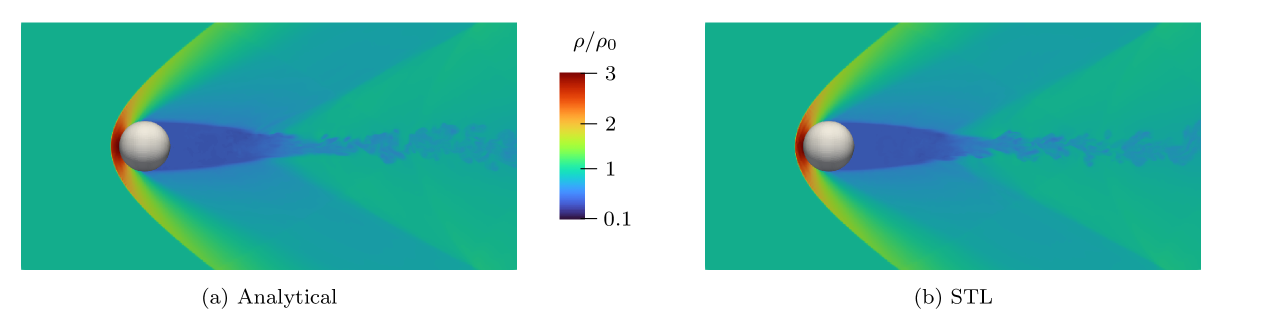
Figure 1: Steady density field ($\rho/\rho_{0}$) of Mach 2 helium flow over a sphere with (a) analytical level set and (b) STL-based level set.

4.1.3 Phase change: First order transition, liquid–vapor

The phase change model for $N$ fluids is integrated into MFC implemented by introducing disequilibrium terms for pressure ($p$), temperature ($T$), and chemical potential ($\mu$) into $\bm{s}(\bm{q})$ in 9. This inclusion increases system stiffness, making a fractional-step method essential [36, 37, 4]. In the case of infinitely fast relaxation, the governing PDEs can be replaced with nonlinear, lower-dimensional, algebraic relations. For example, for the $pT$-relaxation, we have [38]

$$f(p)=\sum_{i=1}^{N}\alpha_{i}-1=\sum_{i=1}^{N}\frac{\gamma_{i}-1}{\gamma_{i}}\frac{\alpha_{i}\rho_{i}c_{p,i}}{\sum_{j=1}^{N}\alpha_{j}\rho_{j}c_{p,j}}\frac{\rho e+p-\sum_{j=1}^{N}\alpha_{j}\rho_{i}e_{*,i}}{\sum_{i=1}^{N}\alpha_{i}\rho_{i}c_{p,i}}-1=0,$$

and for the $pTg$-relaxation

$$F_{1}\left(\alpha_{1}\rho_{1},p\right)=A+\frac{B}{T}+C\ln(T)+D\ln(p+\pi_{\infty,1})-\ln(p+\pi_{\infty,2})=0,$$

and

$$F_{2}\left(\alpha_{1}\rho_{1},p\right)=\rho e+p+\alpha_{1}\rho_{1} (e_{*,2}-e_{*,1})-\alpha_{m}\rho_{m}e_{*,2}$$

$$-\sum_{i=3}^{N}\alpha_{i}\rho_{i}q_{i}+ T\big{[}\alpha_{1}\rho_{1}(c_{p,2}-c_{p,1})-\alpha_{m}\rho_{m}c_{p,2}-\sum_{i=3}^{N}\alpha_{i}\rho_{i}c_{p,i}\big{]}=0,$$

in which $T=T\left(\alpha_{1}\rho_{1},p\right)$ is the relaxed temperature

$$T\left(\alpha_{1}\rho_{1},p\right)=\left\{\alpha_{1}\rho_{1}\left[\frac{c_{p,1}-c_{v,1}}{p+\pi_{\infty,1}}-\frac{c_{p,2}-c_{v,2}}{p+\pi_{\infty,2}}\right]+\alpha_{m}\rho_{m}\left[\frac{c_{p,2}-c_{v,2}}{p+\pi_{\infty,2}}\right]+\sum_{i=3}^{N}\left[\alpha_{i}\rho_{i}\frac{c_{p,i}-c_{v,i}}{p+\pi_{\infty,i}}\right]\right\}^{-1},$$

with $\alpha_{m}\rho_{m}=\alpha_{1}\rho_{1}+\alpha_{2}\rho_{2}$ and $e_{*,i}$ an energy reference parameter added to the stiffened gas EOS (see section 2.2) internal energy equation for species $i$. Subscripts $(\,\cdot\,)_{1,2}$ indicate the reacting liquid and vapor. The remaining subscripts are the inert phases. $A$, $B$, $C$, and $D$ are fluid-dependent parameters [4]. These strategies are compatible with five- and six-equation models and are solved via Newton’s method. Once the solution is obtained, the solver advances to the next time step.

4.1.4 Euler–Euler sub-grid bubble dynamics

We model Euler–Euler sub-grid models for bubble dynamics using the method of classes and the method of moments. The method of classes is based on the ensemble phase-averaged equations [39], which can be used to represent dispersions of radially oscillating bubbles as well as other particles [40, 41, 42, 43]. The void fraction of the dispersed phase $\alpha$ is assumed to be negligible compared to the liquid phase ($\alpha_{l}$) under dilute assumptions. The bubbles are represented statistically via random variables $R$, $\dot{R}$, and $R_{o}$ corresponding to the instantaneous bubble radius, time derivative, and equilibrium bubble radius. The mixture-averaged pressure field is

$$p(\bm{x},t)=(1-\alpha)p_{\ell}+\alpha\left(\frac{\overline{R^{3}p_{bw}}}{\overline{R^{3}}}-\rho\frac{\overline{R^{3}\dot{R}^{2}}}{\overline{R^{3}}}\right),$$

where $p_{bw}$ is the associated bubble wall pressure and $p_{\ell}(\bm{x},t)$ is the liquid pressure according to the modified stiffened-gas EOS [44]:

$$\Gamma_{\ell}p_{\ell}+\Pi_{\infty,\ell}=\frac{1}{1-\alpha}\left(E-\frac{1}{2}\rho\bm{u}^{2}\right).$$

The bubble pressure $p_{b}$ follows the polytropic assumption, and the bubble wall pressure $p_{bw}$ is

$$p_{bw}=p_{o}\left(\frac{R_{o}}{R}\right)^{3\gamma}-\frac{4\mu\dot{R}}{R}-\frac{2\sigma}{R}.$$

The bubble number density per unit volume $n_{\mathrm{bub.}}(\bm{x},t)$ is conserved as

$$\frac{\partial n_{\mathrm{bub.}}}{\partial t}+\nabla\cdot(n_{\mathrm{bub.}}\bm{u})=0.$$

For the spherical bubbles considered here, $n_{\mathrm{bub.}}$ is related to the void fraction $\alpha$ via

$$\alpha(\bm{x},t)=\frac{4}{3}\pi{\overline{R^{3}}}n_{\mathrm{bub.}}(\bm{x},t),$$

and so the void fraction $\alpha(\bm{x},t)$ transports as

$$\frac{\partial\alpha}{\partial t}+\bm{u}\cdot\nabla\alpha=3\alpha\frac{\overline{R^{2}\dot{R}}}{\overline{R^{3}}},$$

the right-hand side represents the change in void fraction due to bubble growth and collapse. The over-barred terms appearing in the above equations denote average quantities of the bubble dispersion. These are averaged over $N_{\mathrm{bin}}$ bins of $R_{o}$ using a log-normal probability distribution function (pdf). We implement the Rayleigh–Plesset and Keller–Miksis equations [45] for the radial bubble dynamics. The Keller–Miksis dynamics are

$$R\ddot{R}\left(1-\frac{\dot{R}}{c}\right)+\frac{3}{2}\dot{R}^{2}\left(1-\frac{\dot{R}}{3c}\right)=\frac{p_{\mathrm{bw}}-p_{l}}{\rho_{l}}\left(1+\frac{\dot{R}}{c}\right)+\frac{R\dot{p}_{\mathrm{bw}}}{\rho c}.$$

The method of classes incorporates stochasticity in $R_{o}$ using a log-normal pdf (probability density function). However, modeling complex bubbly flow phenomena requires the expansion of the set of stochastic variables, including instantaneous bubble variables. Moreover, the inaccuracy of the polytropic assumption can limit the scope of its applications. The method of moments is used for this purpose, which employs a population balance equation (PBE) to govern the pdf of the bubbles. The pdf $f(R,\dot{R},R_{o})$ governs the moments $\mu_{lmn}$ as

$$\mu_{lmn}=\overline{R^{l}\dot{R}^{m}R_{o}^{n}}=\int_{\Omega}R^{l}\dot{R}^{m}R_{o}^{n}f(R,\dot{R},R_{o})\,\text{d}R\text{d}\dot{R}\text{d}R_{o},$$

The moments are evaluated using a conditional inversion procedure that follows Fox et al. [46]. The conditional probability density function $f(R,\dot{R}|R_{o})$ without coalescence or breakup effects is governed by the PBE

$$\frac{\partial f}{\partial t}+\frac{\partial}{\partial R}(f\dot{R})+\frac{\partial}{\partial\dot{R}}(f\ddot{R})=0.$$

The evolution of the raw moments $\vec{\bm{\mu}}$ is obtained by integrating the population balance equation. The set of transport equations for $\vec{\bm{\mu}}$ are

$$\frac{\partial n_{\mathrm{bub.}}\mu_{i}}{\partial t}+\nabla\cdot(n_{\mathrm{bub.}}\mu_{i}\bm{u})=n_{\mathrm{bub.}}{\dot{\mu}_{i}}=n_{\mathrm{bub.}}g_{i},$$ (12)

which are enumerated over each moment and corresponding right-hand side of the column vectors $\vec{\bm{\mu}}$ and $\bm{g}$, denoted as $\mu_{i}$ and $g_{lmn}$. So,

$$g_{lmn}=l\mu_{l-1,m+1,n}+m\iiint_{\Omega}\ddot{R}R^{l}\dot{R}^{m-1}R_{o}^{n}f(\vec{\bm{\mu}})\,\text{d}R\text{d}\dot{R}\text{d}R_{o},$$

and $\Omega=\Omega_{R}\times\Omega_{\dot{R}}\times\Omega_{R_{o}}=(0,\infty)\times(-\infty,\infty)\times(0,\infty)$ [42]. The integral is computed via quadrature nodes obtained by the inversion procedure.

The pdf is conditioned on $R_{o}$ as

$$f(R,\dot{R},R_{o})=f(R,\dot{R}|R_{o})f(R_{o}),$$

and the raw moments are

$$\mu_{lmn}\equiv\int_{\Omega_{R_{o}}}f(R_{o})R_{o}^{m}\mu_{lm}(R_{o})\,\text{d}R_{o}\approx\sum_{i=1}^{N_{R_{o}}}w_{i}\widehat{R}_{o,i}^{n}\,\mu_{lm}(\widehat{R}_{o,i}),$$

where $N_{R_{o}}$ represents the polydispersity of the bubble population. The conditional moments $\mu_{lm}$ are evaluated using a conditional hyperbolic inversion procedure (CHyQMOM). The CHyQMOM algorithm is described in Fox et al. [46], and a detailed discussion of application to bubble dynamics is in Bryngelson et al. [41]. The total moments follow as

$$\mu_{lmn}=\sum_{i=1}^{N_{R_{o}}}w_{i}\widehat{R}_{o,i}^{n}\sum_{j=1}^{N_{R}}\sum_{k=1}^{N_{\dot{R}}}\left[\widehat{w}_{j,k}\widehat{R}_{j}^{l}\widehat{\dot{R}}_{k}^{m}\right]_{\widehat{R}_{o,i}},$$

These moments evaluate the right-hand side of the moment evolution equation and the ensemble-phase averaged terms. The evaluation of $\overline{R^{3}p_{bw}}$ requires the accounting of statistics of $p_{b}$. Without polytropic assumptions, this requires including additional internal variables in the PBE. The ODEs for $p_{b}$ and $m_{v}$ are initialized using an isothermal assumption and evolved at the quadrature nodes, keeping computation costs low. This strategy assumes their probability densities to be Dirac delta functions centered at the quadrature nodes for $R$ and $\dot{R}$. The ODEs for $p_{b}$ and $m_{v}$ follow Ando et al. [47] as

$$\dot{p}_{b}=\frac{3\gamma_{b}}{R}\left(-\dot{R}p_{b}+R_{v}T_{bw}\dot{m_{v}}+\frac{\gamma_{b}-1}{\gamma_{b}}k_{bw}\frac{\partial T}{\partial r}\Bigr{|}_{\begin{subarray}{c}r=R\end{subarray}}\right)\quad\text{and}\quad\dot{m}_{v}=\frac{D\rho_{bw}}{1-\chi_{vw}}\frac{\partial\chi_{vw}}{\partial r}\Bigr{|}_{\begin{subarray}{c}r=R\end{subarray}}.$$

4.1.5 Euler–Lagrange sub-grid bubble dynamics

The Euler–Lagrange model for sub-grid bubble dynamics is based on the volume-averaged equations of motion and describes the dynamics of a mixture of dispersed bubbles in a compressible liquid. Mixture properties $\overline{(\cdot)}$ are defined as $\overline{(\cdot)}=(1-\alpha)(\cdot)_{l}+\alpha(\cdot)_{g}$, where $\alpha$ is the volume fraction of the gas or void fraction, and the subscripts $l$ and $g$ denote the liquid and gas phase, respectively. Assuming zero slip-velocity between the liquid and gas phase and applying the volume averaging yield the following set of inhomogeneous equations

$$\frac{\partial\rho_{l}}{\partial t}+\nabla\cdot\left(\rho_{l}\bm{u}_{l}\right) =\frac{\rho_{l}}{1-\alpha}\left[\frac{\partial\alpha}{\partial t}+\bm{u}_{l}\cdot\nabla\alpha\right],$$ (13)

$$\frac{\partial\left(\rho_{l}\bm{u}_{l}\right)}{\partial t}+\nabla\cdot\left(\rho_{l}\bm{u}_{l}\otimes\bm{u}_{l}+p\mathcal{I}-\mathcal{T}_{l}\right) =\frac{\rho_{l}\bm{u}_{l}}{1-\alpha}\left[\frac{\partial\alpha}{\partial t}+\bm{u}_{l}\cdot\nabla\alpha\right]-\frac{\alpha\nabla\cdot\left(p\mathcal{I}-\mathcal{T}_{l}\right)}{1-\alpha},$$

$$\frac{\partial E_{l}}{\partial t}+\nabla\cdot\left(\left(E_{l}+p\right)\bm{u}_{l}-\mathcal{T}_{l}\cdot\bm{u}_{l}\right) =\frac{E_{l}}{1-\alpha}\left[\frac{\partial\alpha}{\partial t}+\bm{u}_{l}\cdot\nabla\alpha\right]-\frac{\alpha\nabla\cdot\left(p\bm{u}_{l}-\mathcal{T}_{l}\cdot\bm{u}_{l}\right)}{1-\alpha}.$$

Here, $\mathcal{T}_{l}$ is the viscous stress tensor of the liquid host. The advantage of the above form of equations is that the left-hand side of the equation can be seen as the conservation equations for the liquid phase (the details of which are explained in section 2.1.1), and the right-hand side part can be seen as source terms that carry the effect of the bubbles in the host liquid.

The volumetric oscillations of the sub-grid bubbles due to pressure variations in the surrounding medium are modeled using the Keller–Miksis equation of section 4.1.4. The Lagrangian field equation is integrated using a fourth-order accurate Runge–Kutta scheme with adaptive time-stepping.

MFC communicates the bubble sizes to the carrier-flow solver via the local void fraction $\alpha$. This coupling is achieved by computing an effective void fraction derived from the contribution of each bubble to its surrounding computational cells, which is illustrated in fig. 2.

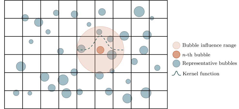
Figure 2: Volume spreading of the $n$-th bubble for the void fraction computations using a Gaussian kernel of characteristic radial extent (not to scale).

The bubble volume is smeared in the continuous field of the void fraction in the mixture at its coordinate $\bm{x}_{n}$ using a regularization kernel $\delta$ as

$$\alpha(\bm{x})=\sum_{n=1}^{N_{\mathrm{bub}}}V_{n}\delta=\left(\frac{4}{3}\pi R_{n}^{3}\right)\delta,$$ (14)

where $N_{\mathrm{bub}}$ is the number of bubbles, and $V_{n}$ is the volume of bubble $n$. We use the continuous, second-order, truncated Gaussian function for the kernel. With $\alpha$, all the terms on the right-hand side of 13 can be computed. More details on the numerical implementation can be found in Maeda and Colonius [9] and Fuster and Colonius [48].

4.1.6 Fluid–elastic structure interaction

Fluid–structure interaction with hypoelastic materials is modeled by adding the elastic shear stress $\bm{T}^{e}$ to the Cauchy stress tensor of the five-equation and six-equation models described in section 2.1.1 and section 2.1.2, respectively. The model relies on transforming strains to strain rates using the Lie objective temporal derivative [49, 50]. The strain rates are computed using high-order accurate central finite differences. The mixture energy is also updated to include the elastic contribution, which gives

$$E=e+\frac{\lVert\bm{u}\rVert^{2}}{2}+\frac{\bm{T}^{e}:\bm{T}^{e}}{4\rho G},$$

where $G$ is the shear modulus of the medium. The third term on the right-hand side is the hypoelastic energy term. The Lie objective temporal derivative of the elastic stresses

$$\dot{\bm{T}}^{e}=\frac{D\bm{T}^{e}}{Dt}-\bm{l}\cdot\bm{T}^{e}-\bm{T}^{e}\cdot\bm{l}^{\top}+\bm{T}^{e}\operatorname{tr}(\bm{D}),$$

where $\bm{l}$ is the velocity gradient, and for an isotropic Kelvin–Voigt material $\dot{\bm{T}}^{e}=2G\bm{D}^{d}$ [51] are used to derive a time evolution equation for the elastic stresses. Here, the deviatoric component of the velocity gradient is $\bm{D}^{d}=\bm{D}-\mathrm{tr}(\bm{D})\bm{I}/3$. Appending this evolution equation to the five-equation model gives the five-equation model with hypoelasticity

$$\frac{\partial\alpha_{i}\rho_{i}}{\partial t}+\nabla\cdot(\alpha_{i}\rho_{i}\bm{u}) =0,$$

$$\frac{\partial\rho\bm{u}}{\partial t}+\nabla\cdot(\bm{u}\otimes\bm{u}+p\bm{I}-\bm{T}^{e}) =\nabla\cdot\bm{T}^{v},$$

$$\frac{\partial\rho E}{\partial t}+\nabla\cdot\left[(\rho E+p)\bm{u}-\bm{T}^{e}\cdot\bm{u}\right] =\nabla\cdot(\bm{T}^{v}\cdot\bm{u}),$$

$$\frac{\partial\alpha_{i}}{\partial t}+\bm{u}\cdot\nabla\alpha_{i} =K\nabla\cdot\bm{u},$$

$$\frac{\partial(\rho\bm{T}^{e})}{\partial t}+\nabla\cdot\left(\rho\bm{T}^{e}\otimes\bm{u}\right) =\bm{S}^{e},$$

where $\bm{S}^{e}$ is the elastic source term:

$$\bm{S}^{e}=\rho\left(\bm{l}\cdot\bm{T}^{e}+\bm{T}^{e}\cdot\bm{l}^{\top}-\bm{T}^{e}\operatorname{tr}(\bm{D})+2G\bm{D}^{d}\right).$$

Details of the hypoelastic model implementation can be found in Spratt [52].

Fluid–structure interaction with hyperelastic materials is modeled with an evolution equation for the reference map using the reference map technique (RMT) of [53]. The gradient of the reference map $\bm{\xi}$, the inverse of the deformation gradient $\bm{F}$,

$$\bm{F}=\left(\nabla\bm{\xi}\right)^{-1},$$

is computed using a high-order central finite-difference scheme. The evolution equation of the reference map is combined with the conservation of mass equation to obtain a conservative form,

$$\frac{\partial\left(\rho\bm{\xi}\right)}{\partial t}+\nabla\cdot\left(\rho\bm{\xi}\otimes\bm{u}\right)=\bm{0},$$

and solved with the system of equations in sections 2.1.1 and 2.1.2. The deformation gradient $\bm{F}$, the left Cauchy–Green strain $\bm{b}$,

$$\bm{b}=\bm{F}\bm{F}^{\top},$$

and the elastic deviatoric contribution to the Cauchy stress tensor $\bm{T}^{e}$ are computed. For a compressible neo-Hookean material model, the elastic deviatoric part of the Cauchy stress tensor is

$$\bm{T}^{e}=\frac{G}{J}\left(\bm{b}-\frac{1}{3}\operatorname{tr}(\bm{b})\bm{I}\right),$$

where $J$ is the determinant of $\bm{b}$ and $\bm{I}$ is the identity tensor and the hyperelastic energy is $e^{e}=G\left(I_{b}-3\right)/2$, where $I_{b}$ is the first invariant of $\bm{b}$. Further details of the hyperelastic model implementation can be found in Barbosa et al. [54].

4.1.7 Chemical reactions and combustion

High-fidelity simulations of reacting flows are critical to designing efficient propulsion systems. Such simulations require models for the effects that chemical reactions have on the flow. There are two major differences with respect to simulations of inert flow. First, mixture composition varies locally due to chemical reactions, and as a result, fluid properties, like viscosity, do as well. This effect must be accounted for to achieve acceptable accuracy; it is typically achieved using transport equations for individual species. Second, because chemical reactions release heat, temperature changes can become substantial, so variable thermodynamic properties are needed for accuracy. As we expand in what follows, we now incorporate these effects through detailed models in the gas phase.

The gas phase is a mixture of $N_{\mathrm{species}}$ species with mass fractions $\{Y_{m}\}_{m=1}^{N_{\mathrm{species}}}$. Without molecular transport, these evolve as

$$\frac{\partial\rho_{g}Y_{m}}{\partial t}+\frac{\partial\rho_{g}u_{i}Y_{m}}{\partial x_{i}}=W_{(m)}\dot{\omega}_{m},\quad m=1,\dots,N_{\mathrm{species}},$$

where $\rho_{g}$ is the density of the gas phase, $W_{m}$ is the molecular weight of the $m^{\mathrm{th}}$ species (with parenthesized subscript obviating Einstein summation) and $\dot{\omega}_{m}$ its net production rate by chemical reactions—the chemical source term.

Next, we provide detailed expressions for the chemical source term. Their implementation uses code generation and is discussed in section 4.3.7. We simulate gas-phase combustion by integrating section 4.1.7 along with the equations for conservation of momentum and total energy density section 2.1.1. Plans to extend this capability to multi-phase combustion with liquid or solid fuels entail the implementation of detailed expressions for phase changes [55, 56, 57].

The net production rate in section 4.1.7 is

$$\dot{\omega}_{m}=\sum_{n=1}^{N_{\mathrm{species}}}(\nu_{mn}^{\prime\prime}-\nu_{mn}^{\prime})R_{n},\quad m=1,\dots,N_{\mathrm{species}},$$ (15)

where $\nu_{mn}^{\prime},\,\nu_{mn}^{\prime\prime}$ are the forward and reverse stoichiometry of the $m^{\mathrm{th}}$ species in the $n^{\mathrm{th}}$ reaction, and $R_{n}$ the net reaction rate of progress. By the law of mass action,

$$R_{n}=k_{n}(T)\Bigg{[}\prod_{j=1}^{N}\Bigg{(}\frac{\rho_{g}Y_{j}}{W_{j}}\Bigg{)}^{\nu_{jn}^{\prime}}-\frac{1}{K_{n}(T)}\prod_{k=1}^{N}\Bigg{(}\frac{\rho_{g}Y_{k}}{W_{k}}\Bigg{)}^{\nu_{kn}^{\prime\prime}}\Bigg{]}$$ (16)

where $k_{n}$ and $K_{n}$ are the rate coefficient and the equilibrium constant. Expressions for the rate coefficient are reaction-dependent but conventionally take a modified Arrhenius form

$$k_{n}(T)=A_{n}T^{b_{n}}\exp(-T_{a,n}/T),$$ (17)

where $A_{n},\,b_{n},\,T_{a,n}$ are the pre-exponential factor, temperature exponent, and activation temperature of the $n^{\mathrm{th}}$ reaction. The equilibrium constant in 16 is determined from standard equilibrium thermodynamics; detailed expressions can be found elsewhere [58, 59].

As stated, the effects of combustion on mixture thermodynamics must also be accounted for. For the equation of state, we assume a mixture of ideal gases, so

$$p=\rho R_{u}T/W,$$ (18)

where $R_{u}$ is the universal gas constant and

$$W=\Bigg{(}\sum_{m=1}^{N_{\mathrm{species}}}\frac{Y_{m}}{W_{m}}\Bigg{)}^{-1}$$ (19)

is the mixture molecular weight. The temperature follows from

$$e_{g}-\sum_{m=1}^{N_{\mathrm{species}}}e_{m}(T)\,Y_{m}=0,$$ (20)

where $e_{g}$ is the gas-phase internal energy per unit mass (obtained from section 2.1.1), and $\{e_{m}(T)\}_{m=1}^{N_{\mathrm{species}}}$ the species internal energies. These are

$$e_{m}(T)=\frac{\hat{h}_{m}(T)-R_{u}T}{W_{m}},\qquad m=1,\dots,N_{\mathrm{species}},$$ (21)

where $\{\hat{h}_{m}(T)\}_{m=1}^{N_{\mathrm{species}}}$ are the species molar enthalpies, modeled using NASA polynomials [60]:

$$\frac{\hat{h}_{m}}{R_{u}T}=\frac{\hat{C}_{0}}{T}+\sum_{r=1}^{5}\frac{\hat{C}_{r}}{r}T^{r-1},$$ (22)

with fit coefficients $\{\hat{C}\}_{r=0}^{5}$ determined from experiments and collision integrals [61]. The fitting procedure for 22 includes heats of formation so, in concert with 20 and 21, it accounts for combustion heat release. In practice, to obtain the temperature, 20 is solved iteratively using a standard Newton method.

To validate our implementation, we simulate a one-dimensional reacting shock tube and reproduce the published results of Martínez-Ferrer et al. [62]. We uniformly discretize the domain of size $L=$12\text{\,}\mathrm{cm}\text{/}$$ with 400 grid cells. The left boundary represents a reflecting wall, while the right boundary is an outflow. Reactions are modeled using the San Diego mechanism [63]. The shock travels left, reflects from the wall, and ignites the mixture. The combustion wave and the shock coalesce into a detonation wave. The comparison between our implementation and the results of Martínez-Ferrer et al. [62] is shown in fig. 3. The agreement is sufficient for validation, given the uncertainties due to different numerics and combustion mechanisms.

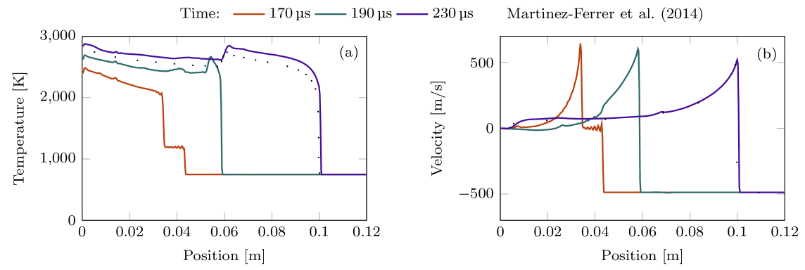
Figure 3: (a) Temperature and (b) velocity profiles of a one-dimensional reactive shock tube compared to the results of Martínez-Ferrer et al. [62].

4.1.8 Surface tension at diffuse material interfaces

Surface tension for two-fluid flows is implemented using the model of Schmidmayer et al. [64]. An advection equation for the color function $c$, which is $0$ in one fluid and $1$ in the other, is added to the system of equations. This color function is then used to calculate the capillary stress tensor

$$\bm{\Omega}=-\sigma\left(\lVert\nabla c\rVert\bm{I}-\frac{\nabla c\otimes\nabla c}{\lVert\nabla c\rVert}\right),$$

where $\sigma$ is the surface tension coefficient. The capillary stress tensor defines the contribution of surface tension to the momentum and mixture energy equations. The six-equation model with surface tension is

$$\frac{\partial\alpha_{i}\rho_{i}}{\partial t}+\nabla\cdot(\alpha_{i}\rho_{i}\bm{u}) =0,$$

$$\frac{\partial\rho\bm{u}}{\partial t}+\nabla\cdot(\rho\bm{u}\bm{u}+p\bm{I}+\bm{\Omega}-\bm{T}^{v}) =0,$$

$$\frac{\partial\alpha_{1}\rho_{1}e_{1}}{\partial t}+\nabla\cdot(\alpha_{1}\rho_{1}e_{1}\bm{u})+\alpha_{1}p_{1}\cdot\nabla\bm{u} =-\mu p_{I}(p_{2}-p_{1})-\alpha_{1}\bm{T}_{1}^{v}:\nabla\bm{u},$$

$$\frac{\partial\alpha_{2}\rho_{2}e_{2}}{\partial t}+\nabla\cdot(\alpha_{1}\rho_{2}e_{2}\bm{u})+\alpha_{2}p_{2}\cdot\nabla\bm{u} =-\mu p_{I}(p_{1}-p_{2})-\alpha_{2}\bm{T}_{2}^{v}:\nabla\bm{u},$$

$$\frac{\partial(\rho E+\varepsilon_{0})}{\partial t}+\nabla\cdot\left((\rho E+\varepsilon_{0}+P)\bm{u}+(\bm{\Omega}-\bm{T}^{v})\cdot\bm{u}\right) =0,$$

$$\frac{\partial\alpha_{1}}{\partial t}+\bm{u}\cdot\nabla\alpha_{1} =\mu(p_{1}-p_{2}),$$

$$\frac{\partial c}{\partial t}+\bm{u}\cdot\nabla c =0,$$

where $\varepsilon_{0}$ is the capillary mixture energy. The six-equation model with surface tension is conservative, except for the pressure relaxation terms, and follows the second law of thermodynamics. This model has been validated against analytic solutions to the Laplace pressure jump and experimental results for shock droplet interaction [64].

4.2 Numerical methods

4.2.1 General characteristic boundary conditions

The priority for time-dependent boundary conditions for hyperbolic equations requires a smooth egress of the outgoing artifacts with a minimal effect on the interior solution. For this purpose, the non-reflecting characteristic boundary conditions [32] are used, which performs a characteristic decomposition of the governing equation at the boundary. Ignoring the contribution of the viscous and transverse terms, this is

$$\frac{\partial q_{c}}{\partial t}+R_{x}\Lambda_{x}L_{x}\frac{\partial q_{c}}{\partial x}=0,$$

where $q_{c}$ is the set of conservative variables, $\Lambda_{x}=\operatorname{diag}(\lambda_{j})=\operatorname{diag}(u-c,u,u,u,u+c)$ are the eigenvalues of the Jacobian, and $R_{x}$ and $L_{x}$ are the right and left eigenvectors. The contribution of the characteristics can be further decomposed into incoming and outgoing waves depending on the sign of the eigenvalue as

$$\lambda_{j}^{i}=\lambda_{j}-n_{x}|\lambda_{j}|\quad\text{and}\quad\lambda_{j}^{o}=\lambda_{j}+n_{x}|\lambda_{j}|,$$

with $n_{x}=1$ for the right boundary and $n_{x}=-1$ for the left boundary. The non-reflecting characteristic boundary conditions subsequently ignore the contribution of the incoming wave to get

$$\frac{\partial q_{c}}{\partial t}=-R_{x}\Lambda^{o}_{x}L_{x}\frac{\partial q_{c}}{\partial x}.$$

In many applications, the primitive variables $q_{p}$ outside the computational domain are not known, necessitating a more general approach. The evolution equation for the conservative variables at the boundary can be cast into primitive form as

$$\frac{\partial q_{c}}{\partial t}=-R_{x}\Lambda_{x}L_{x}\frac{\partial q_{c}}{\partial x}=-R_{x}\Lambda_{x}L_{x}P\frac{\partial q_{p}}{\partial x},$$

where $P=\partial_{q_{p}}q_{c}$ is the conversion Jacobian matrix. The characteristics $\bm{\mathcal{L}}=\Lambda_{x}L_{x}P\partial_{x}q_{p}$ are

$$\mathcal{L}_{1} =(u-c)\left(\frac{\partial p}{\partial x}-\rho c\frac{\partial u}{\partial x}\right),\quad\mathcal{L}_{2}=u\left(c^{2}\frac{\partial\rho}{\partial x}-\frac{\partial p}{\partial x}\right),$$

$$\mathcal{L}_{3} =u\frac{\partial v}{\partial x},\quad\mathcal{L}_{4}=u\frac{\partial w}{\partial x},\quad\mathcal{L}_{5}=(u+c)\left(\frac{\partial p}{\partial x}+\rho c\frac{\partial u}{\partial x}\right),$$

with $v$ and $w$ being the transverse velocities. The generalized characteristic boundary conditions make use of the solution outside the domain at ghost points ($q_{p}^{\mathrm{(g)}}$) to incorporate the contribution of the incoming characteristics [65]. The characteristics $\bm{\mathcal{L}}$ in this case are

$$\bm{\mathcal{L}}=-\Lambda^{o}_{x}L_{x}\frac{\partial q_{c}}{\partial x}-\Lambda^{i}_{x}L_{x}\frac{\partial q_{c}}{\partial x}=-\Lambda^{o}_{x}L_{x}\frac{\partial q_{c}}{\partial x}+n_{x}\lambda_{x}^{i}L_{x}P\frac{(q_{p}^{\mathrm{(g)}}-q_{p})}{\Delta}$$

where $\Delta$ is the grid spacing between the boundary ($q_{p}$) and the ghost point ($q_{p}^{\mathrm{(g)}}$). In practice, $\Delta$ is set to be the grid spacing between the boundary and the first interior point for accuracy and stability. For a subsonic outflow at the right boundary, coefficients $\mathcal{L}^{i}_{2}$ through $\mathcal{L}^{i}_{5}$ are set to $0$ as these correspond to outgoing waves. The incoming characteristic $\mathcal{L}^{i}_{1}$ is calculated as

$$\mathcal{L}_{1}^{i}=(u-c)((p^{\mathrm{(g)}}-p)-\rho c(u^{\mathrm{(g)}}-u)),$$

where $p^{\mathrm{(g)}}$ and $u^{\mathrm{(g)}}$ are the pressure and normal velocity in the exterior of the domain.

4.2.2 WENO-Z, TENO, and high-order non-uniform reconstruction

The WENO-Z scheme [66] enhances classical WENO methods by improving their spectral properties while being faster than WENO-M. The $(2k-1)$-th order WENO-Z weight $\omega_{r}^{(\mathrm{Z})}$ for the $r$-th stencil is computed as

$$\omega_{r}^{(\mathrm{Z})}=\frac{\alpha_{r}}{\sum_{i=0}^{k-1}\alpha_{i}},\quad\alpha_{r}=d_{r}\left(1+\left(\frac{\tau}{\beta_{r}+\epsilon}\right)^{q}\right),\quad\tau=\left|\beta_{0}-\beta_{k-1}\right|,$$

where $d_{r}$ are the ideal weights, $\tau$ is the global smoothness indicator, and the parameter $q$ (typically set to $1$ for fifth-order reconstruction) influences the convergence rate at the critical points and the spectral properties. This formulation applies to schemes of order 3, 5, and 7.

The Targeted Essentially Non-Oscillatory (TENO) scheme further reduces numerical dissipation by employing a stencil selection process similar to the ENO method [67]. A $K$-th order accurate TENO scheme uses $K-2$ candidate stencils of increasing width. Its equations are given by

$$\omega_{r}^{(\mathrm{T})}=\frac{d_{r}\delta_{r}}{\sum_{i=0}^{K-3}d_{i}\delta_{i}},\quad\delta_{r}=\begin{cases}0,&\text{ if }\chi_{r}<C_{T}\\ 1,&\text{ otherwise }\end{cases},\quad\chi_{r}=\frac{\gamma_{r}}{\sum_{i=0}^{K-3}\gamma_{i}},\quad\gamma_{r}=d_{r}\left(1+\frac{\tau}{\beta_{r}+\epsilon}\right)^{6},$$

where $C_{T}$ is a smoothness threshold for stencil activation and $\tau$ is defined as in the WENO-Z scheme.

The explicit expressions for the seventh-order WENO reconstruction in our code are omitted here due to their considerable length. Instead, we present a generalized approach for reconstructing a $(2k-1)$-order scheme from cell averages on non-uniform grids. For each stencil, the reconstruction polynomial is obtained using the Lagrange interpolation method [68]:

$$p(x)=\sum_{j=0}^{k-1}\hskip 5.0pt\underbrace{\Delta x_{j}\sum_{m=j+1}^{k}\left(\frac{\sum_{\begin{subarray}{c}l=0\\ l\neq m\end{subarray}}^{k}\prod_{\begin{subarray}{c}q=0\\ q\neq m,\,l\end{subarray}}^{k}\left(x-x_{q-\frac{1}{2}}\right)}{\prod_{\begin{subarray}{c}l=0\\ l\neq m\end{subarray}}^{k}\left(x_{m-\frac{1}{2}}-x_{l-\frac{1}{2}}\right)}\right)}_{\mbox{$c_{j}(x)$}}\hskip 5.0ptf_{j}.$$

Here, $x_{j}$ denotes cell-center location, $x_{j+1/2}$ the cell-boundary location, and $\Delta x_{j}:=x_{j+1/2}-x_{j-1/2}$ is the cell width. For each stencil $r=0,1,\dots,k-1$, the $k$-cell stencil spans the interval from $x_{-1/2}$ to $x_{k-1/2}$. Consequently, the overall $(2k-1)$-cell stencil is centered at $x_{k-r-1}$, and the right flux is $p_{r}:=p(x_{k-r-1/2})$.

To reduce computational cost, we rewrite $p(x)$ in terms of the differences $\Delta f_{j}:=f_{j+1}-f_{j}$, so that $p(x)=\sum_{j=0}^{k-2}\hat{c}_{j}(x)\Delta f_{j}+f_{0}$. For flux evaluation at $x_{k-r-1/2}$, the coefficients $\hat{c}_{r,j}:=\hat{c}_{j}(x_{k-r-1/2})$ for each $\Delta f_{j}$ and stencil $r$ are precomputed at the start of the program.

The smoothness indicator for stencil $r$ is defined by

$$\beta_{r}=\sum_{l=1}^{k-1}\Delta x_{k-r-1}^{2l-1}\int_{x_{k-r-\frac{3}{2}}}^{x_{k-r-\frac{1}{2}}}\left(\frac{\partial^{l}p(x)}{{\partial x}^{l}}\right)^{2}\text{d}x.$$

Rewriting this in terms of the difference formulation yields

$$\beta_{r}=\sum_{j=0}^{k-2}\sum_{m=j}^{k-2}\hskip 5.0pt\underbrace{\left(2-\delta_{jm}\right)\sum_{l=1}^{k-1}\Delta x_{k-r-1}^{2l-1}\int_{x_{k-r-\frac{3}{2}}}^{x_{k-r-\frac{1}{2}}}\frac{\partial^{l}\hat{c}_{j}(x)}{{\partial x}^{l}}\frac{\partial^{l}\hat{c}_{m}(x)}{{\partial x}^{l}}\text{d}x}_{\mbox{$\hat{b}_{r,j,m}$}}\hskip 5.0pt\Delta f_{j}\Delta f_{m},$$

where $\delta_{jm}$ is the Kronecker delta. The coefficients $\hat{b}_{r,j,m}$ for each cross term $\Delta f_{j}\Delta f_{m}$ and stencil $r$ are precomputed. Reformulating in terms of $\Delta f$ reduces the number of terms from $k$ to $k-1$ for $p_{r}$, and from $k(k+1)/2$ to $(k-1)k/2$ for $\beta_{r}$, thereby reducing the computational cost.

4.2.3 Strang splitting for stiff sub-grid dynamics

Sub-grid bubbles often exhibit rapid dynamics, necessitating a small time step for stable computation of the bubble source term. When the time scale of the background flow significantly exceeds that of the sub-grid bubbles, fully resolving the temporal dynamics becomes computationally prohibitive. To address this, we implement the Strang splitting scheme, which separates the time integration of the background flow and the sub-grid bubbles [69]. The implementation supports a single resolved phase with sub-grid bubbles governed by

$$\frac{\partial\bm{q}}{\partial t}=\nabla\cdot\bm{F}(\bm{q})+\bm{s}(\bm{q}).$$

The Strang splitting scheme integrates the equation over one time step by integrating 3 sub-equations for $\bm{q}^{*}$, $\bm{q}^{**}$, and $\bm{q}^{***}$ as

$$\frac{\partial\bm{q}^{*}}{\partial t} =\bm{s}(\bm{q}),\quad t \in[0,\Delta t/2],\quad \bm{q} {}^{*}(0)=\bm{q}^{n},$$

$$\frac{\partial\bm{q}^{**}}{\partial t} =-\nabla\cdot\bm{F}(\bm{q}^{**}),\quad t \in[0,\Delta t],\quad \bm{q} {}^{**}(0)=\bm{q}^{*}(\Delta t/2),$$

$$\frac{\partial\bm{q}^{***}}{\partial t} =\bm{s}(\bm{q}^{***}),\quad t \in[0,\Delta t/2],\quad \bm{q} {}^{***}(0)=\bm{q}^{**}(\Delta t),\quad\bm{q}^{n+1}=\bm{q}^{***}(\Delta t/2).$$

To solve for $\bm{q}^{*}$ and $\bm{q}^{***}$, where the stiff bubble source term is evaluated, we use a third-order accurate embedded Runge–Kutta scheme with adaptively controlled step sizes [70]. The step size, $h$, is updated based on the estimated error, $\bm{e}$, calculated as

$$\bm{q}^{n+1} =\bm{q}^{n}+\frac{h}{6}\left(k_{1}+k_{2}+4k_{3}\right),$$

$$\hat{\bm{q}}^{n+1} =\bm{q}^{n}+\frac{h}{8}\left(3k_{1}+3k_{2}+2k_{3}\right),$$

$$\bm{e} =\bm{q}^{n+1}-\hat{\bm{q}}^{n+1}=-\frac{5}{24}h\left(k_{1}+k_{2}-2k_{3}\right),$$

where $k_{1}=\partial\bm{q}^{n}/\partial t$, $k_{2}=\partial\bm{q}^{(1)}/\partial t$, and $k_{3}=\partial\bm{q}^{(2)}/\partial t$. Here, $\bm{q}^{n+1}$ represents a solution of the third-order TVD Runge–Kutta scheme, and $\hat{\bm{q}}^{n+1}$ is a 2nd-order accurate solution obtained using the same $k_{1}$, $k_{2}$, and $k_{3}$ that requires minimal additional computational cost. More details of the adaptive step size control algorithm can be found in Hairer et al. [70].

4.2.4 Low-Mach number treatment

Godunov-type Riemann solvers, including the HLLC Riemann solver, are known to lose their accuracy at low Mach numbers due to numerical dissipation in the discrete solution [71]. To address this limitation, we use two numerical treatments based on the approaches of Thornber et al. [72] and Chen et al. [73], allowing users to select their preferred scheme.

Thornber et al. [72] proposed a simple modification to the reconstructed velocities of the left and right states as

$$u_{\mathrm{L}}^{*} =\frac{u_{\mathrm{L}}+u_{\mathrm{R}}}{2}+z\frac{u_{\mathrm{L}}-u_{\mathrm{R}}}{2},$$

$$u_{\mathrm{R}}^{*} =\frac{u_{\mathrm{L}}+u_{\mathrm{R}}}{2}+z\frac{u_{\mathrm{R}}-u_{\mathrm{L}}}{2},$$

$$z =\mbox{min}\left(\mbox{max}\left(\frac{\lvert u_{\mathrm{L}}\rvert}{c_{\mathrm{L}}},\frac{\lvert u_{\mathrm{R}}\rvert}{c_{\mathrm{R}}}\right),1\right),$$

where the modified velocities $u_{\mathrm{L}}^{*}$ and $u_{\mathrm{R}}^{*}$ replace the original velocities $u_{\mathrm{L}}$ and $u_{\mathrm{R}}$ in the calculation of the signal velocity and fluxes. This strategy ensures the correct scaling of the pressure and density fluctuations in the low Mach number regime.

On the other hand, Chen et al. [73] identified a source term, $p_{d}$, which is responsible for the wrong scaling at the low Mach number limit. To address this, they proposed an anti-dissipation pressure correction (APC) term, which is incorporated into the flux calculation. For the HLLC Riemann solver, the terms $p_{d}$ and APC are

$$p_{d} =\frac{\rho_{\mathrm{L}}\rho_{\mathrm{R}}(S_{\mathrm{L}}-u_{\mathrm{L}})(S_{\mathrm{R}}-u_{\mathrm{R}})(u_{\mathrm{R}}-u_{\mathrm{L}})}{\rho_{\mathrm{R}}(S_{\mathrm{R}}-u_{\mathrm{R}})-\rho_{\mathrm{L}}(S_{\mathrm{L}}-u_{\mathrm{L}})},$$

$$\mathrm{APC}_{\rho u} =(z-1)p_{d}\left(n_{x},n_{y},n_{z}\right)^{\top},$$

$$\mathrm{APC}_{\rho E} =(z-1)p_{d}S_{*},$$

$$z =\mbox{min}\left(\mbox{max}\left(\frac{\lvert u_{\mathrm{L}}\rvert}{c_{\mathrm{L}}},\frac{\lvert u_{\mathrm{R}}\rvert}{c_{\mathrm{R}}}\right),1\right).$$

Here, $\mathrm{APC}_{\rho u}$ and $\mathrm{APC}_{\rho E}$ represent the correction terms for the momentum and energy equations, respectively, and $n_{x}$, $n_{y}$, and $n_{z}$ denote the components of the unit normal vector. Then, the corrected HLLC flux is

$$\bm{F}^{\mathrm{HLLC+APC}}=\begin{cases}\bm{F}\left(\bm{q}^{\mathrm{(L)}}\right)&S_{\mathrm{L}}\geq 0,\\ \bm{F}^{(*\mathrm{L})}+\bm{APC}&S_{\mathrm{L}}\leq 0\leq S_{*},\\ \bm{F}^{(*\mathrm{R})}+\bm{APC}&S_{*}\leq 0\leq S_{\mathrm{R}},\\ \bm{F}\left(\bm{q}^{(\mathrm{R})}\right)&0\geq S_{\mathrm{R}}.\end{cases}$$

4.3 Software and high-performance computing

4.3.1 GPU Offloading with OpenACC on NVIDIA and AMD Hardware

Vendor portable GPU offloading on AMD and NVIDIA hardware is implemented using OpenACC [74]. OpenACC is a directive-based tool that allows the developer to generate GPU kernels by adding directive clauses around developer-identified regions of parallelism in the code. OpenACC is supported by NVIDIA’s NVHPC compiler for use with NVIDIA GPUs and HPE’s Cray Compiler Environment for use with both NVIDIA and AMD GPUs. Other compilers, like GNU 14+ and Flang 18+, support OpenACC, though their relative immaturity at time of writing makes them insufficient to support MFC.

LABEL:lst:kernel shows an example of a typical GPU kernel in MFC. The outer loops over j, k, and l iterate through $\mathcal{O}(100)$ elements each, corresponding to the grid cells in the MPI subdomain. The inner loop over i iterates through each equation in the current model. For two-phase flow problems this loop spans $\mathcal{O}(1)$ elements. When additional features like hypo- and hyperelasticity or chemistry are added to the problem, the extent of this inner loop can be $\mathcal{O}(10)$.

OpenACC describes parallelism using terminology in which gangs, workers, and vectors refer to blocks, warps, and threads in CUDA notation. By default, when OpenACC encounters a parallel loop clause, it distributes the workload across gangs, leaving each gang to utilize a single vector. Appending the gang vector clause to the parallel loop tells the compiler to split the work across multiple gangs with a fixed vector length, which more efficiently uses available resources and increases execution speed. Appending collapse(3) to the three outer loops instructs the compiler to collapse those three loops and select the optimal gang and vector sizes based on the current problem and architecture. Our tests show that serialization of the innermost loop i increases performance, in part due to its relatively small range.

Listing 1: Directive setup for a typical MFC OpenACC kernel.

⬇

!$acc parallel loop vector gang collapse(3) &

!$acc default(present) private(...)

do l = 0, p ! Third coordinate direction

do k = 0, n ! Second coordinate direction

do j = 0, m ! First coordinate direction

!$acc loop seq

do i = 1, num_PDEs

! << Core kernel here, O(100) arithmetic operations >>

end do

end do

end do

end do

!$acc end parallel loop

MFC also uses NVIDIA and AMD’s vendor-provided libraries cuTensor and hipBLAS to perform hardware-optimized array reshaping for coalescing memory before the most expensive kernels. Memory coalescence before the WENO reconstruction and approximate Riemann solver kernels results in a ten-fold speedup due to the increased throughput of high-bandwidth memory. cuTENSOR [75] performs similarly to fully collapsed OpenACC loops on NVIDIA hardware, providing only marginal speedup. hipBLAS [76] performs array transposes approximately seven times faster than fully collapsed OpenACC loops. NVIDIA and CCE’s cuFFT [77] and hipFFT [78] perform fast Fourier transforms on GPU devices and FFTW [79] is used for CPU-based simulations. Code encased by OpenACC host_data use_device and end host_data clauses executed are on the GPU using these vendor-provided libraries, reducing the need for hardware-specific optimizations.

4.3.2 Performance on various CPU, GPU, and APU architectures

MFC 5.0 has been benchmarked on a broad range of CPU, GPU, and APU (superchip) devices. LABEL:t:serialperf shows report the single-device performance in terms of its grind time, which is computed as time per grid point, PDE, and right-hand side evaluation. The grind times are calculated for one GPU or APU device or one CPU socket. The benchmarks were performed under a similar strategy as that used on published testbed reports [80]. These quantities are for a typical, representative compressible multi-component problem: 3D, inviscid, 5-equation model problem with two advected species (8 PDEs) and 8M grid points (158-cubed 3D uniform grid). The equation is solved via fifth-order accurate WENO finite volume reconstruction and the HLLC approximate Riemann solver. This case is in the MFC source code under examples/3D_performance_test. One can execute it via

⬇

./mfc.sh run examples/3D_performance_test/case.py -t pre_process simulation --case--optimization -n <num_cores_or_gpus> -j <num_build_threads>

One can execute this command for CPU cases, which builds an optimized version of the code for this case, then executes it. For benchmarking GPU devices, one will likely want to use -n <num_gpus> where the usual case for single GPU device benchmarking leaves <num_gpus> as unity. Similar performance is also seen for other problem configurations, such as the Euler equations (4 PDEs). All results are for the compiler that gave the best performance, including AOCC, Intel, GCC, CCE, and NVHPC.

CPU results may be performed on CPUs with more cores than reported in LABEL:t:serialperf; we report results for the best performance given the full processor die by checking the performance for different core counts on that device. CPU results are the best performance we achieved using a single socket (or die). GPU results are for a single GPU device. For single-precision (SP) GPUs, we performed computation in double-precision via conversion in compiler/software; these numbers are not for single-precision computation. AMD MI250X and MI300A devices have multiple graphics compute dies per socket; we report results for two GCDs for the AMD MI250X and the entire APU (6 XCDs) for the AMD MI300A.

Table 1: Observed grind time performance (time), reported as nanoseconds per grid point per PDE per right-hand side evaluation. Using more GPU devices or CPU sockets may not improve the grind time for the same problem, as the problem will be made smaller per marshaled device (and so grind time is expected to be approximately constant).

Hardware	Type	Usage	Time	Hardware	Type	Usage	Time
NVIDIA GH200	APU	1 GPU	0.32	NVIDIA A10	GPU	1 GPU	4.3
NVIDIA H100 SXM5	GPU	1 GPU	0.38	AMD EPYC 7713	CPU	64 cores	5.0
NVIDIA H100 PCIe	GPU	1 GPU	0.45	Intel Xeon 8480CL	CPU	56 cores	5.0
AMD MI250X	GPU	1 GPU	0.55	Intel Xeon 6454S	CPU	32 cores	5.6
AMD MI300A	APU	1 APU	0.57	Intel Xeon 8462Y+	CPU	32 cores	6.2
NVIDIA A100	GPU	1 GPU	0.62	Intel Xeon 6548Y+	CPU	32 cores	6.6
NVIDIA V100	GPU	1 GPU	0.99	Intel Xeon 8352Y	CPU	32 cores	6.6
NVIDIA A30	GPU	1 GPU	1.1	Ampere Altra Q80-28	CPU	80 cores	6.8
AMD EPYC 9965	CPU	192 cores	1.2	AMD EPYC 7513	CPU	32 cores	7.4
AMD MI100	GPU	1 GPU	1.4	Intel Xeon 8268	CPU	24 cores	7.5
AMD EPYC 9755	CPU	128 cores	1.4	AMD EPYC 7452	CPU	32 cores	8.4
Intel Xeon 6980P	CPU	128 cores	1.4	NVIDIA T4	GPU	1 GPU	8.8
NVIDIA L40S	GPU	1 GPU	1.7	Intel Xeon 8160	CPU	24 cores	8.9
AMD EPYC 9654	CPU	96 cores	1.7	IBM Power10	CPU	24 cores	10
Intel Xeon 6960P	CPU	72 cores	1.7	AMD EPYC 7401	CPU	24 cores	10
NVIDIA P100	GPU	1 GPU	2.4	Intel Xeon 6226	CPU	12 cores	17
Intel Xeon 8592+	CPU	64 cores	2.6	Apple M1 Max	CPU	10 cores	20
Intel Xeon 6900E	CPU	192 cores	2.6	IBM Power9	CPU	20 cores	21
AMD EPYC 9534	CPU	64 cores	2.7	Cavium ThunderX2	CPU	32 cores	21
NVIDIA A40	GPU	1 GPU	3.3	Arm Cortex-A78AE	CPU	16 cores	25
Intel Xeon Max 9468	CPU	48 cores	3.5	Intel Xeon E5-2650V4	CPU	12 cores	27
NVIDIA Grace CPU	CPU	72 cores	3.7	Apple M2	CPU	8 cores	32
NVIDIA RTX6000	GPU	1 GPU	3.9	Intel Xeon E7-4850V3	CPU	14 cores	34
AMD EPYC 7763	CPU	64 cores	4.1	Fujitsu A64FX	CPU	48 cores	63
Intel Xeon 6740E	CPU	92 cores	4.2

fig. 4 shows the roofline performance for the most expensive kernels on NVIDIA and AMD accelerators. At the time of writing, roofline analysis is unavailable on the MI300A APU, and so is not shown. NVHPC 24.5 compilers and NVIDIA Nsight Compute profilers produce roofline results on NVIDIA devices, and CCE 18 with Omniperf profile the roofline on the AMD MI250X GPU. The WENO and approximate Riemann kernels achieve 37% and 14% of peak performance on the NVIDIA A100. On the NVIDIA GH200, the WENO and approximate Riemann kernels achieve 24% and 5% of peak compute performance. The AMD MI250X achieves 22% of peak compute performance in the WENO kernel and 3% of peak performance in the approximate Riemann problem.

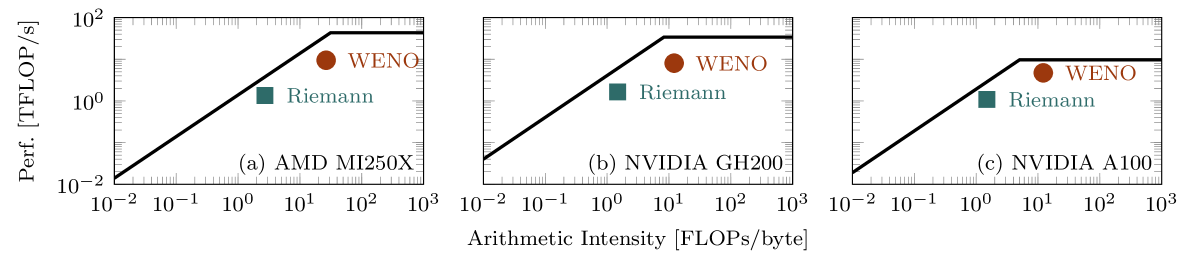
Figure 4: The roofline performance of the fifth-order accurate WENO reconstruction and HLLC approximate Riemann solve kernels on the AMD MI250X, NVIDIA GH200, and NVIDIA A100.

The breakdown of time spent in the two most expensive kernels, time spent packing arrays, and time spent doing all other computations and communication is shown in fig. 5. The WENO and approximate Riemann kernels take up just over 50% of the total time on NVIDIA GPUs. On AMD GPU devices, the time spent in the WENO and approximate Riemann kernels is similar to that of NVIDIA devices. Still, these kernels make up about a third of the total wall time due to an increase in time spent packing arrays for coalesced memory access. The profiles show a high number of cache misses on the AMD MI250X, which we expect is be due to the smaller device caches than that of to the shown NVIDIA device.

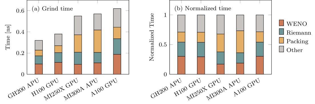
Figure 5: Grind time and normalized breakdown of the most expensive kernels, array packing, and all other computations on NVIDIA (GH200, H100, A100) and AMD (MI250X, MI300A) GPUs/APUs.

4.3.3 Exascale capabilities and beyond

MFC efficiently scales to tens of thousands of GPUs on the world’s fastest computers. Figure 6 shows the weak scaling performance of MFC on OLCF Summit (now retired) with NVIDIA V100 GPUs, OLCF Frontier with AMD MI250X GPUs, and LLNL El Capitan with AMD MI300A APUs. MFC scales to 13824 NVIDIA V100 GPUs on OLCF Summit with 97% efficiency, to 65536 AMD MI250X GCDs (32768 MI250X GPUs) on OLCF Frontier with 95% efficiency, and to 196608 AMD MI300As XCDs (32768 MI300A APUs) on LLNL El Capitan.

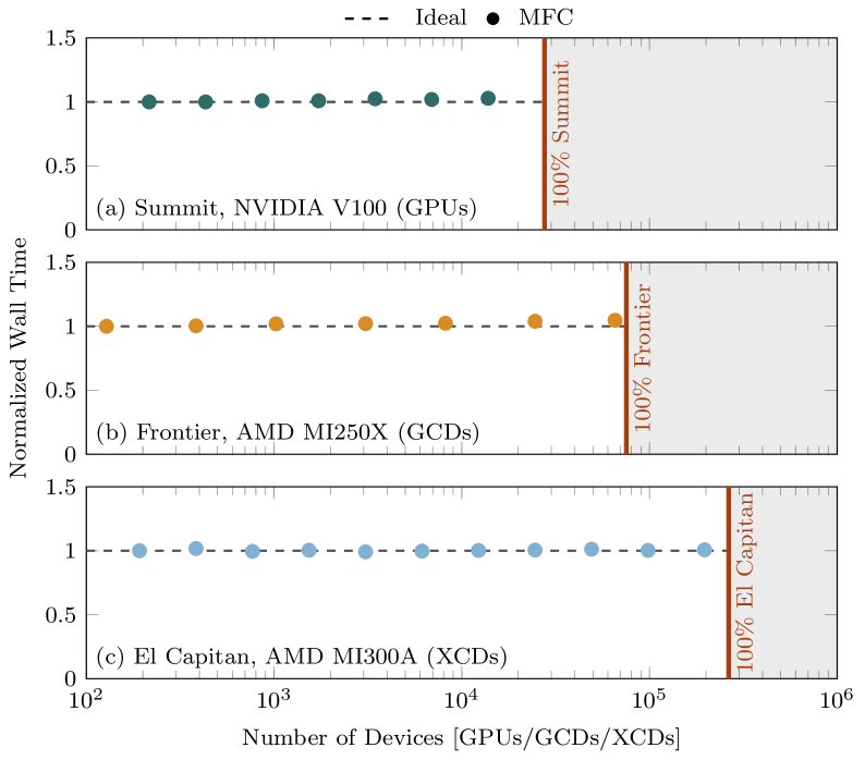
Figure 6: Weak scaling results on OLCF Summit and Frontier and LLNL El Capitan. MFC Scales from 128 to 13824 NVIDIA V100 GPUs with 97% efficiency on Summit, from 128 to 65536 AMD MI250Xs (GCDs) with 95% efficiency on Frontier, and 192 to 196608 AMD MI300As (XCDs) with 99% efficiency on El Capitan (XCDs).

The communication patterns in MFC also result in high strong scaling efficiencies. Figure 7 shows the strong scaling performance of MFC on OLCF Summit and OLCF Frontier and compares weak scaling with and without GPU-aware MPI. The problem sizes in fig. 7 (a) correspond to approximately 100% and 50% usage of available GPU memory per device in the base case. In the base case, with 8M grid cells per device, strong scaling efficiencies of 79% and 51% are observed on OLCF Summit when increasing the device count by a factor of 8 or 16 without GPU-aware MPI. For the case with 32 million grid cells per device in the base case, strong scaling efficiencies of 81% and 77% when increasing the device count by a factor of 8 and 16 without GPU-aware MPI. The higher efficiencies seen with the AMD MI250X on OLCF Frontier are partly due to the larger problem size’s increased computation-to-communication ratio and the improved internode communication on Frontier. With GPU-aware MPI, the strong scaling efficiencies on OLCF Summit increase to 84% and 60% when increasing the device count by a factor of 8 and 16. On Frontier, the efficiencies are 96% and 92% when the device count is increased by the same factors.

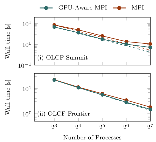
(a) Strong scaling	(b) GPU-aware MPI enhancement

Figure 7: Strong scaling performance on OLCF Summit and OLCF Frontier. The figures on the left show the strong scaling performance for a species problem without using GPU-aware MPI. The quantities in (b) indicate the number of grid cells per device in the base case. The figures in (b) show the improvement in scaling performance when GPU-aware MPI is used. In (b), an 8M grid point case is used for benchmarking MFC on (i) Summit, and a 32M grid point case is used for (ii) Frontier. The number of processes is commensurate with Summit’s NVIDIA V100 GPUs or Frontier’s AMD MI250X GPUs.

4.3.4 Parallel I/O at extreme scales

Parallel I/O is implemented using the MPI I/O library to facilitate shared file parallel I/O and file-per-process parallel I/O. Shared file parallel I/O was sufficient for handling up to 10K processes, but a significant slowdown in I/O times was observed when scaling to over 65K processes on OLCF Frontier. For simulations that use over 10K processes, each process writes a file for each I/O operation. To alleviate the file system pressure resulting from metadata creation for tens of thousands of files, MFC accesses the file system in waves of 128 processes separated by a fixed number of floating point operations.

4.3.5 Software resilience and continuous integration

Each pull request to MFC goes through a suite of continuous integration actions. The correctness, performance, and code quality are evaluated through this continuous integration suite. MFC’s test suite of over 300 cases is compiled and run using GNU and Intel compilers on MacOS and Ubuntu operating systems on CPUs on GitHub runners via GitHub actions. The same tests are run using NVHPC on CPUs and NVIDIA GPUs and with CCE on AMD GPUs via self-hosted runners. All of these tests are compared to the same set of golden files to ensure that the code in the main branch of MFC provides the same results on CPUs and GPUs, regardless of compiler or operating system. The coverage of the test suite is evaluated using Codecov to help ensure coverage of the test suite for additional (or removed) code. Each pull request is benchmarked against the MFC master branch on CPUs and GPUs to prevent performance regressions; it also checks for compiler warnings and formatting to ensure code consistency.

4.3.6 Metaprogramming

Metaprogramming is implemented using the Fortran preprocessor Fypp [81]. Fypp is a Python-based preprocessor that is used to inline subroutines via programmer directives and collapse repetitive code. MFC uses Fypp for several tasks, including automation of deep copies of derived types for allocation on the GPU device. NVIDIA’s NVHPC Fortran compiler automatically allocates derived types on the device, but CCE adheres closer to the OpenACC technical specification (3.2 at the time of writing) and requires manual allocation. If one holds many host variables, this process is cumbersome. Instead, we use the code in LABEL:lst:deepCopy to inline the source code via @:ACC_SETUP_VFs(var1,var2,…,varN) after allocating the vector fields var1,var2,…,varN on the host. This macro performs deep copies, reducing the number of lines required to initialize the variables at runtime.

Listing 2: A Fortran+Fypp macro that manually deep copies derived types from the host to the device.

⬇

#:def acc_setup_vfs(\*args)

block

integer :: macros_setup_vfs_i

#:for arg in args

!$acc enter data copyin(${arg}$)

!$acc enter data copyin(${arg}$%vf)

if (allocated(${arg}$%vf)) then

do macros_setup_vfs_i = lbound(${arg}$%vf, 1), ubound(${arg}$%vf, 1)

if (associated(${arg}$%vf(macros_setup_vfs_i)%sf)) then

!$acc enter data copyin(${arg}$%vf(macros_setup_vfs_i))

!$acc enter data create(${arg}$%vf(macros_setup_vfs_i)%sf)

end if

end do

end if

#:endfor

end block

#:enddef

Fypp simplifies module initialization by wrapping allocate and deallocate into macros that allocate the variable and perform the enter data create required when using OpenACC for GPU offloading. LABEL:lst:memManag shows an example macro. Variables are allocated and deallocated using @:ALLOCATE(var1,var2,…,varN) and @:DEALLOCATE(var1,var2,…,varN). The code length is further reduced by using Fypp to abstract away repetitive code via preprocessor loops [82].

Listing 3: An Fypp macro for allocating and initializing a variable with OpenACC.

⬇

#:def ALLOCATE(*args)

allocate (${’, ’.join(args)}$)

!$acc enter data create(${’, ’.join(args)}$)

#:enddef ALLOCATE

#:def DEALLOCATE(*args)

deallocate (${’, ’.join(args)}$)

!$acc exit data delete(${’, ’.join(args)}$)

#:enddef DEALLOCATE

Metaprogramming sets problem parameters as constant parameters in case files. This option is called case optimization, enabled via the flag --case-optimization at run time. Case optimization reduces register pressure by providing the compiler with the parameters of a configuration. On CPUs, specifying the problem parameters at compile-time results in a two-times speedup of the code. On GPUs, case optimization decreases run time by about a factor of ten. Variables are precriped in a file with the Fypp code #:set var = val. This file is included in the Fortran source code, compile-time-known parameters are declared using the Fypp logic of LABEL:lst:fyppDec.

Listing 4: Fortran+Fypp code the declaration of configuration-specific parameters for compile-time optimization.

⬇

#:if CASE_OPTIMIZATION

integer, parameter :: var = ${var}$

#:else

integer :: var

#:endif

4.3.7 Code generation for efficient reactions and thermodynamics

MFC now simulates chemically reacting flows. We accommodate this feature via combustion routines that evaluate the chemical source terms and species thermodynamics. Comprehensive libraries, such as Cantera, provide such routines. However, these exist in a different compilation unit to the flow solver, so they cannot easily be offloaded via the OpenACC directive-based strategy of section 4.3.1. We address this challenge through code generation, producing a computational representation of thermochemistry at the same abstraction level as MFC’s compressible flow solver. This strategy obviates the need to optimize comprehensive combustion libraries at link time. MFC uses Pyrometheus [58, 83] for code generation, generating thermochemistry code in OpenACC-decorated Fortran.

Pyrometheus is based on a symbolic representation of the combustion formulation that takes mechanism parameters from Cantera. The symbolic representation is mapped to a user-specified target language. For Fortran, the generated code is a module that can be easily integrated and offloaded with MFC. The mapping process decorates the routines with OpenACC statements for GPU offloading, so the generated code does not need to be modified a posterior. The generated code unrolls inner loops over species and reactions and prepares compile-time constants such as Arrhenius parameters. This optimization meaningfully reduces kernel runtime [83]. In a similar vein to case optimization of section 4.3.6, Pyrometheus assigns compile-time-known bounds to the arrays in the generated code, enabling optimization of register allocations and decreasing runtime by about a factor of 5 for GPU kernels.

Pyrometheus is verified against Cantera, though it is itself thoroughly tested. The testing suite is language-agnostic, so the generated Fortran code is as accurate as a C-based alternative. The generated code is mechanism-specific, but because code generation is free in comparison with simulation time, multiple mechanisms can be preprocessed. For MFC, we generate code for established combustion mechanisms for hydrogen [63] and methane combustion [84], though we are not limited to these.

5 Example simulations

5.1 Shock–bubble-cloud interaction

The first example simulation shows the interaction between a cloud of $75$ randomly placed $3\text{\,}\mathrm{mm}\text{/}$ bubbles and a shockwave in water. The computational domain is $[-9D,9D]\times[0,10D]\times[0,10D]$ before grid stretching and is discretized as $(N_{x},N_{y},N_{z})=(2000,1000,1000)$, or about 2B grid points. The grid points are stretched away from the bubbles to avoid boundary effects via

$$x_{\mathrm{stretch}}=x+\frac{x}{a_{x}}\left[\log\left[\cosh\left(\frac{a_{x}(x-x_{a})}{L}\right)\right]+\log\left[\cosh\left(\frac{a_{x}(x-x_{b}}{L}\right)\right]-2\log\left[\cosh\left(\frac{a_{x}(x_{b}-x_{a}}{2L}\right)\right]\right],$$

where $a_{x}$ is the stretching parameter, $L$ is the domain length, and $x_{a}$ and $x_{b}$ control the stretching location. Figure 8 shows the $\alpha=0.5$ isosurface at increasing points in time from left to right. The detail view shows the grid resolution around one of the collapsing bubbles. The initial condition has 100 uniform-sized grid points across each bubble diameter. The simulation was performed using 1024 AMD MI250X GCDs (512 AMD MI250X GPUs) on OLCF Frontier and completed in approximately $30\text{\,}\mathrm{min}\text{/}$.

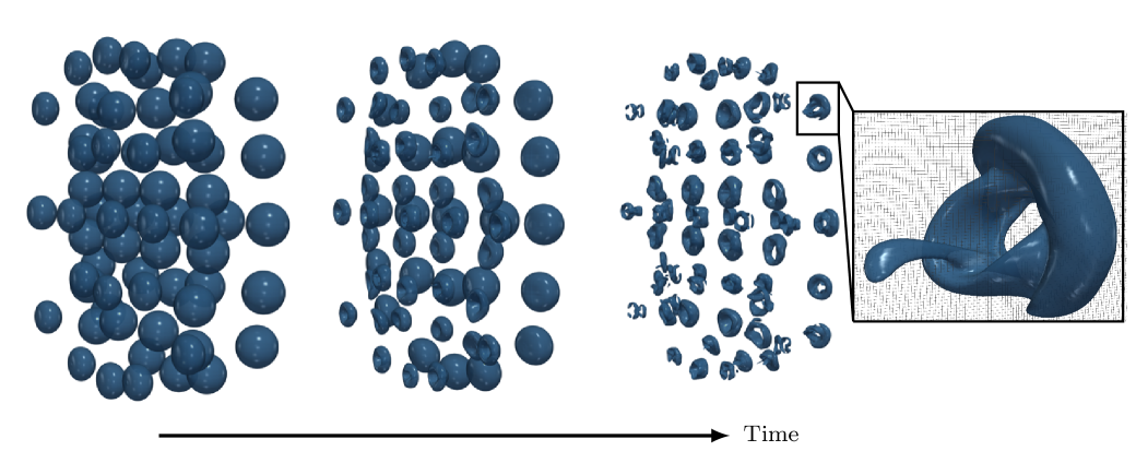
Figure 8: Shock-induced collapse of a cloud of 75 air bubbles in water. The $\alpha=0.5$ contour is shown at increasing points in time from left to right. The magnified view shows the mesh resolution around one of the collapsing bubbles.

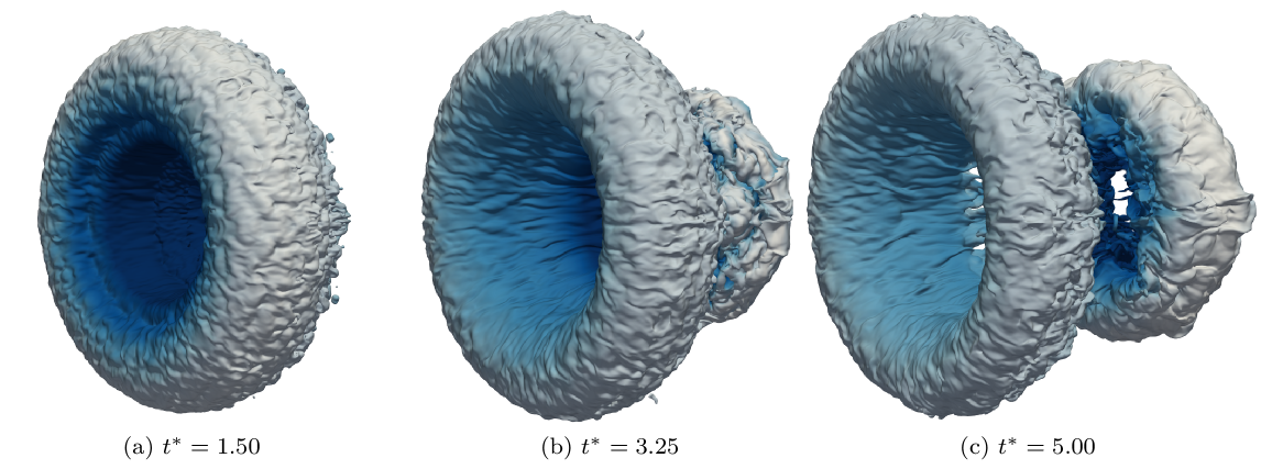
Figure 9: Shock-induced collapse of a helium bubble in air. The $\alpha=0.5$ contour, representing the material interface, is shown at dimensionless times as labeled. The isosurface is colored by its velocity magnitude, with darker colors corresponding to higher velocities. The initial droplet has 640 grid cells across its diameter in each coordinate direction.

5.2 Shock–bubble interaction

The second example simulation shows the interaction between a helium bubble in air impinged by a shock wave. The computational domain has spatial extents $[0,20D]\times[-5D,5D]\times[-5D,5D]$ before grid stretching and is discretized with $(N_{x},N_{y},N_{z})=(3200,1600,1600)$, which is over 8B grid points. The domain boundaries are moved far away from the bubble to avoid boundary effects using grid stretching (described in section 5.1). Figure 9 shows the $\alpha=0.5$ isosurface, which represents the interface between air and helium, at dimensionless times $t^{*}=tU/D=1.5$, $3.25$, and $5.0$ for shock speed $U$ and bubble diameter $D$. The isosurface is colored by velocity magnitude, with darker colors corresponding to higher velocities. The bubble is resolved with 640 grid cells in its initial diameter. The simulation was performed using 144 NVIDIA H200 GPUs in $16\text{\,}\mathrm{h}\text{/}$.

5.3 Taylor–Green vortex

The third example simulation is a $\mbox{\text{Re}}=1600$, $\mbox{\text{Ma}}=0.1$ Taylor–Green vortex. The initial condition follows that of Hillewaert [85]. The computational domain is a cube with side lengths of $L=2\pi$ and is discretized with $N_{x}=N_{y}=N_{z}=1600$, which is approximately 4B grid points. Figure 10 shows the isosurface with zero Q-criterion colored by vorticity magnitude at dimensionless times $t/t_{c}=4$, $12$, and $20,$ with darker colors corresponding to higher vorticity magnitudes. The convective timescale $t_{c}$ is defined as $t_{c}=L/\left(c_{0}\mbox{\text{Ma}}\right),$ where $c_{0}$ is the free stream speed of sound. The simulation was performed using 144 NVIDIA H200 GPUs in $28\text{\,}\mathrm{h}\text{/}$.

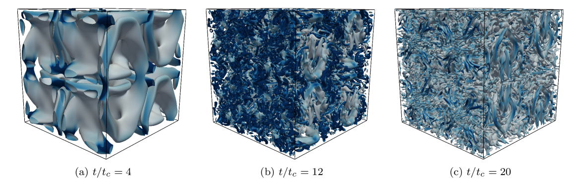
Figure 10: The isosurface with zero Q-criterion of a $\mbox{\text{Re}}=1600$, $\mbox{\text{Ma}}=0.1$ Taylor–Green vortex at dimensionless times $t/t_{c}$ as labeled. The isosurface is colored by the vorticity magnitude, with darker colors corresponding to higher vorticity.

6 Solvers with some shared capabilities

Other open-source codes for CFD exist. These and their relative trade-offs compared to MFC 5.0 are briefly discussed here. URANOS-2.0 (De Vanna and Baldan [86]) is a modern Fortran code that uses OpenACC for GPU offloading to NVIDIA and AMD GPUs. URANOS-2.0 contains some of MFC’s shock-capturing capabilities; it also has compressible turbulence models. STREAmS-2 (Sathyanarayana et al. [87]) is also a Fortran code for compressible flow and uses CUDA Fortran and hipFORT to offload to NVIDIA and AMD GPUs. There is also an OpenMP port of STREAmS-2 that makes it portable to Intel GPUs. AFiD-GPU of Zhu et al. [88] is similar in this context. Neko (Jansson et al. [89]) is a particularly modern object-oriented solver that uses multiple levels of abstraction for offloading to GPUs as well as more extensive extensions for vector processors and FPGAs. The above solvers have offloading capabilities similar to those of MFC, though the physical models and their sophistication differ. MFC offers a broad range of modeling capabilities and numerics for the broad use of multi-phase and -species flows,

7 Conclusion

Since MFC 3.0 [1], the code has transitioned from a specialized research code to an exascale-capable framework for multiphysics and multiphase flows. The implementation of physical models, numerical methods, software infrastructure, and high-performance computing tools embodies this transition.

Version 5.0 introduces six phase-change formulations for vapor–liquid systems and treatments of reacting flows. The implementation extends to non-polytropic sub-grid bubble dynamics models capable of representing sophisticated bubble dynamic processes. Hypo- and hyper-elastic material treatments are now available for solids under large strain rates. A generalized surface tension framework is now included, which is both conservative and numerically robust in our studies.

Numerical advancements accompany MFC’s extended feature set. TENO-6 and WENO-Z shock-capturing schemes meaningfully reduce dispersion error compared to conventional WENO schemes. The Strang-split particle solver maintains second-order temporal accuracy for stiff ODE systems. The implementation of a low-Mach preconditioner reduces numerical dissipation for Mach numbers below $0.1$. A ghost-cell immersed boundary method is now available. This method supports complex 2D and 3D geometries that can be imported as level sets or STL files.

Software infrastructure improvements deliver performance portability across modern architectures. Continuous integration pipelines enforce rigorous quality control through over 300 regression tests, including reproducibility checks across hardware platforms and compilers.

Exascale readiness is demonstrated through multiple performance tests. OpenACC implementations and GPU-aware MPI throughout the codebase enable state-of-the-art strong scaling efficiency on AMD MI250X platforms. Metaprogramming enables a speedup of nearly 10 times over the baseline. Ideal weak scaling behavior is observed for current exascale machines, OLCF Frontier and LLNL El Capitan, which use AMD MI250X GPUs and MI300A APUs, and large-scale NVIDIA-based GPU machines like OLCF Summit and LLNL Lassen.

Declaration of competing interest

The authors declare that they have no known competing financial interests or personal relationships that could have appeared to influence the work reported in this paper.

Statement of data availability

MFC is available in perpetuity under the MIT license at github.com/MFlowCode/MFC.

References

- Bryngelson et al. [2021] S. H. Bryngelson, K. Schmidmayer, V. Coralic, K. Maeda, J. Meng, T. Colonius, MFC: An open-source high-order multi-component, multi-phase, and multi-scale compressible flow solver, Computer Physics Communications 266 (2021) 107396.
- Kapila et al. [2001] A. K. Kapila, R. Menikoff, J. B. Bdzil, S. F. Son, D. S. Stewart, Two-phase modeling of deflagration-to-detonation transition in granular materials: Reduced equations, Physics of Fluids 13 (2001) 3002–3024.
- Allaire et al. [2002] G. Allaire, S. Clerc, S. Kokh, A five-equation model for the simulation of interfaces between compressible fluids, Journal of Computational Physics 181 (2002) 577–616.
- Saurel et al. [2009] R. Saurel, F. Petitpas, R. A. Berry, Simple and efficient relaxation methods for interfaces separating compressible fluids, cavitating flows and shocks in multiphase mixtures, Journal of Computational Physics 228 (2009) 1678–1712.
- Johnsen [2008] E. Johnsen, Numerical Simulations of Non-Spherical Bubble Collapse with Applications to Shockwave Lithotripsy, Ph.D. thesis, California Institute of Technology, 2008.
- Johnsen and Colonius [2006] E. Johnsen, T. Colonius, Implementation of WENO schemes in compressible multicomponent flow problems, Journal of Computational Physics 219 (2006) 715–732.
- Coralic and Colonius [2014] V. Coralic, T. Colonius, Finite-volume WENO scheme for viscous compressible multicomponent flows, Journal of Computational Physics 274 (2014) 95–121.
- Meng [2016] J. C. Meng, Numerical simulations of droplet aerobreakup, Ph.D. thesis, California Institute of Technology, 2016.
- Maeda and Colonius [2018] K. Maeda, T. Colonius, Eulerian–Lagrangian method for simulation of cloud cavitation, Journal of Computational Physics 371 (2018) 994–1017.
- Maeda and Colonius [2017] K. Maeda, T. Colonius, A source term approach for generation of one-way acoustic waves in the Euler and Navier–Stokes equations, Wave Motion 75 (2017) 36–49.
- ACCESS (2025) [Advanced Cyberinfrastructure Coordination Ecosystem: Services and Support] ACCESS (Advanced Cyberinfrastructure Coordination Ecosystem: Services and Support), ACCESS: Advanced cyberinfrastructure coordination ecosystem, https://access-ci.org, 2025. Accessed: 2025-02-14.
- Towns et al. [2014] J. Towns, T. Cockerill, M. Dahan, I. Foster, K. Gaither, A. Grimshaw, V. Hazlewood, S. Lathrop, D. Lifka, G. D. Peterson, R. Roskies, J. R. Scott, N. Wilkins-Diehr, XSEDE: Accelerating scientific discovery, Computing in Science & Engineering 16 (2014) 62–74.
- Pittsburgh Supercomputing Center (2015) [PSC] Pittsburgh Supercomputing Center (PSC), Bridges: A HPC resource for accelerating computational research, https://www.psc.edu/bridges, 2015. Funded by the National Science Foundation under Grant No. OCI-1445606. Retired in 2021.
- Brown et al. [2021] S. T. Brown, P. Buitrago, E. Hanna, S. Sanielevici, R. Scibek, Bridges-2: Transforming research with advanced computational capabilities, Pittsburgh Supercomputing Center (2021).
- San Diego Supercomputer Center (2015) [SDSC] San Diego Supercomputer Center (SDSC), Comet: A petascale supercomputer for the long tail of science, https://www.sdsc.edu/News%20Items/PR20170201_Comet_10k.html, 2015. Accessed: 2025-02-14.
- Strande et al. [2021] S. Strande, H. Cai, M. Tatineni, W. Pfeiffer, C. Irving, A. Majumdar, D. Mishin, R. Sinkovits, M. Norman, N. Wolter, T. Cooper, I. Altintas, M. Kandes, I. Perez, M. Shantharam, M. Thomas, S. Sivagnanam, T. Hutton, Expanse: Computing without boundaries: Architecture, deployment, and early operations experiences of a supercomputer designed for the rapid evolution in science and engineering, Practice and Experience in Advanced Research Computing (PEARC ’21) (2021) 1–8.
- Song et al. [2022] X. C. Song, P. Smith, others, Anvil – System architecture and experiences from deployment and early user operations, in: Practice and Experience in Advanced Research Computing (PEARC ’22), Association for Computing Machinery, New York, NY, USA, 2022, p. 23. doi:10.1145/3491418.3530766.
- National Center for Supercomputing Applications (2022) [NCSA] National Center for Supercomputing Applications (NCSA), Delta: Advanced computing resource for science and engineering, https://delta.ncsa.illinois.edu, 2022. Accessed: 2025-02-14.
- National Center for Supercomputing Applications (2023) [NCSA] National Center for Supercomputing Applications (NCSA), DeltaAI: Expanding AI-focused computing capacity at NCSA, https://deltaai.ncsa.illinois.edu, 2023. Accessed: 2025-02-14.
- Texas Advanced Computing Center (2013) [TACC] Texas Advanced Computing Center (TACC), Stampede: High-performance computing resource at TACC, 2013. Supported by the National Science Foundation under Grant No. OCI-1134872.
- Nystrom and et al. [2017] N. A. Nystrom, et al., Stampede2: The evolution of an XSEDE supercomputer, Proceedings of the Practice and Experience in Advanced Research Computing (PEARC ’17) (2017).
- Texas Advanced Computing Center (2024) [TACC] Texas Advanced Computing Center (TACC), Stampede3: Advanced supercomputing for open science research, https://www.tacc.utexas.edu, 2024. Funded by the National Science Foundation under Award No. 2320757.
- Intel Corporation [2024] Intel Corporation, Intel Developer Cloud: AI-Optimized supercomputing platform, https://console.cloud.intel.com/docs/index.html, 2024. Accessed: 2025-02-14.
- SPEC [2025] SPEC, SPEChpc, https://www.spec.org/products, 2025. Accessed: 2025-02-14.
- Andrianov and Warnecke [2004] N. Andrianov, G. Warnecke, The Riemann problem for the Baer–Nunziato two-phase flow model, Journal of Computational Physics 195 (2004) 434–464.
- Saurel and Pantano [2018] R. Saurel, C. Pantano, Diffuse-interface capturing methods for compressible two-phase flows, Annual Review of Fluid Mechanics 50 (2018) 105–130.
- Schmidmayer et al. [2020] K. Schmidmayer, S. H. Bryngelson, T. Colonius, An assessment of multicomponent flow models and interface capturing schemes for spherical bubble dynamics, Journal of Computational Physics 402 (2020) 109080.
- Menikoff and Plohr [1989] R. Menikoff, B. J. Plohr, The Riemann problem for fluid flow of real materials, Reviews of Modern Physics 61 (1989) 75–130.
- Mohseni and Colonius [2000] K. Mohseni, T. Colonius, Numerical treatment of polar coordinate singularities, Journal of Computational Physics 157 (2000) 787–795.
- Henrick et al. [2005] A. K. Henrick, T. D. Aslam, J. M. Powers, Mapped weighted essentially non-oscillatory schemes: Achieving optimal order near critical points, Journal of Computational Physics 207 (2005) 542–567.
- Toro [1997] E. F. Toro, The HLL and HLLC Riemann Solvers, Springer Berlin Heidelberg, Berlin, Heidelberg, 1997, pp. 293–311.
- Thompson [1990] K. W. Thompson, Time-dependent boundary conditions for hyperbolic systems, II, Journal of Computational Physics 89 (1990) 439–461.
- Gottlieb and Shu [1998] S. Gottlieb, C.-W. Shu, Total variation diminishing Runge–Kutta schemes, Mathematics of Computation 67 (1998) 73–85.
- Tseng and Ferziger [2003] Y.-H. Tseng, J. H. Ferziger, A ghost-cell immersed boundary method for flow in complex geometry, Journal of Computational Physics 192 (2003) 593–623.
- Weiler [1986] K. J. Weiler, Topological structures for geometric modeling (Boundary representation, manifold, radial edge structure), Ph.D. thesis, Rensselaer Polytechnic Institute, 1986.
- Strang [1968] G. Strang, On the construction and comparison of difference schemes, SIAM Journal on Numerical Analysis 5 (1968) 506–517.
- Zein et al. [2010] A. Zein, M. Hantke, G. Warnecke, Modeling phase transition for compressible two-phase flows applied to metastable liquids, Journal of Computational Physics 229 (2010) 2964–2998.
- Flåtten et al. [2011] T. Flåtten, A. Morin, S. T. Munkejord, On solutions to equilibrium problems for systems of stiffened gases, SIAM Journal on Applied Mathematics 71 (2011) 41–67.
- Zhang and Prosperetti [1994] D. Z. Zhang, A. Prosperetti, Ensemble phase‐averaged equations for bubbly flows, Physics of Fluids 6 (1994) 2956–2970.
- Bryngelson et al. [2019] S. H. Bryngelson, K. Schmidmayer, T. Colonius, A quantitative comparison of phase-averaged models for bubbly, cavitating flows, International Journal of Multiphase Flow 115 (2019) 137–143.
- Bryngelson et al. [2023] S. H. Bryngelson, R. O. Fox, T. Colonius, Conditional moment methods for polydisperse cavitating flows, Journal of Computational Physics 477 (2023) 111917.
- Bryngelson et al. [2020] S. H. Bryngelson, A. Charalampopoulos, T. P. Sapsis, T. Colonius, A Gaussian moment method and its augmentation via LSTM recurrent neural networks for the statistics of cavitating bubble populations, International Journal of Multiphase Flow 127 (2020) 103262.
- Bryngelson and Colonius [2020] S. H. Bryngelson, T. Colonius, Simulation of humpback whale bubble-net feeding models, Journal of the Acoustical Society of America 147 (2020) 1126–1135.
- Menikoff and Plohr [1989] R. Menikoff, B. J. Plohr, The Riemann problem for fluid-flow of real materials, Reviews of Modern Physics 61 (1989) 75–130.
- Plesset and Prosperetti [1977] M. S. Plesset, A. Prosperetti, Bubble dynamics and cavitation, Annual Review of Fluid Mechanics. 9 (1977) 145–185.
- Fox et al. [2018] R. O. Fox, F. Laurent, A. Vié, Conditional hyperbolic quadrature method of moments for kinetic equations, Journal of Computational Physics 365 (2018) 269–293.
- Ando et al. [2009] K. Ando, T. Colonius, C. E. Brennen, Improvement of acoustic theory of ultrasonic waves in dilute bubbly liquids, Journal of the Acoustical Society of America 126 (2009) El69–El74.
- Fuster and Colonius [2011] D. Fuster, T. Colonius, Modelling bubble clusters in compressible liquids, Journal of Fluid Mechanics 688 (2011) 352–389.
- Altmeyer et al. [2015] G. Altmeyer, E. Rouhaud, B. Panicaud, A. Roos, R. Kerner, M. Wang, Viscoelastic models with consistent hypoelasticity for fluids undergoing finite deformations, Mechanics of Time-Dependent Materials 19 (2015) 375–395.
- Altmeyer et al. [2016] G. Altmeyer, B. Panicaud, E. Rouhaud, M. Wang, A. Roos, R. Kerner, Viscoelasticity behavior for finite deformations, using a consistent hypoelastic model based on Rivlin materials, Continuum Mechanics and Thermodynamics 28 (2016) 1741–1758.
- Rodriguez and Johnsen [2019] M. Rodriguez, E. Johnsen, A high-order accurate five-equations compressible multiphase approach for viscoelastic fluids and solids with relaxation and elasticity, Journal of Computational Physics 379 (2019) 70–90.
- Spratt [2024] J.-S. Spratt, Numerical Simulations of Cavitating Bubbles in Elastic and Viscoelastic Materials for Biomedical Applications, Ph.D. thesis, California Institute of Technology, 2024.
- Kamrin et al. [2012] K. Kamrin, C. H. Rycroft, J.-C. Nave, Reference map technique for finite-strain elasticity and fluid–solid interaction, Journal of the Mechanics and Physics of Solids 60 (2012) 1952–1969.
- Barbosa et al. [2024] M. C. Barbosa, M. R. Jr., J. Yang, High-fidelity numerical simulations of inertial microbubble collapse at a gel-water interface with finite elasticity and phase change, in: Center for Turbulence Research, Proceedings of the Summer Program, 2024, pp. 349–359.
- Aiyer and Meneveau [2020] A. Aiyer, C. Meneveau, Coupled population balance and large eddy simulation model for polydisperse droplet evolution in a turbulent round jet, Physical Review Fluids 5 (2020) 114305.
- Ren et al. [2021] Y. Ren, J. Cai, H. Pitsch, Theoretical single-droplet model for particle formation in flame spray pyrolysis, Energy & Fuels 35 (2021) 1750–1759.
- Zeng et al. [2002] W. R. Zeng, S. F. Li, W. K. Chow, Review on chemical reactions of burning poly(methyl methacrylate) PMMA, Journal of Fire Sciences 20 (2002) 401–433.
- Cisneros-Garibay et al. [2022] E. Cisneros-Garibay, C. Pantano, J. B. Freund, Flow and combustion in a supersonic cavity flameholder, AIAA Journal (2022) 1–12.
- Al-Khateeb et al. [2009] A. N. Al-Khateeb, J. M. Powers, S. Paolucci, A. J. Sommese, J. A. Diller, J. D. Hauenstein, J. D. Mengers, One-dimensional slow invariant manifolds for spatially homogenous reactive systems, The Journal of Chemical Physics 131 (2009).
- McBride [2002] B. J. McBride, NASA Glenn Coefficients for Calculating Thermodynamic Properties of Individual Species, National Aeronautics and Space Administration, John H. Glenn Research Center, 2002.
- Gardiner [1984] W. Gardiner, Combustion Chemistry, Springer New York, 1984.
- Martínez-Ferrer et al. [2014] P. J. Martínez-Ferrer, R. Buttay, G. Lehnasch, A. Mura, A detailed verification procedure for compressible reactive multicomponent Navier–Stokes solvers, Computers & Fluids 89 (2014) 88–110.
- Saxena and Williams [2006] P. Saxena, F. A. Williams, Testing a small detailed chemical-kinetic mechanism for the combustion of hydrogen and carbon monoxide, Combustion and Flame 145 (2006) 316–323.
- Schmidmayer et al. [2017] K. Schmidmayer, F. Petitpas, E. Daniel, N. Favrie, S. Gavrilyuk, A model and numerical method for compressible flows with capillary effects, Journal of Computational Physics 334 (2017) 468–496.
- Pirozzoli and Colonius [2013] S. Pirozzoli, T. Colonius, Generalized characteristic relaxation boundary conditions for unsteady compressible flow simulations, Journal of Computational Physics 248 (2013) 109–126.
- Borges et al. [2008] R. Borges, M. Carmona, B. Costa, W. S. Don, An improved weighted essentially non-oscillatory scheme for hyperbolic conservation laws, Journal of Computational Physics 227 (2008) 3191–3211.
- Fu et al. [2016] L. Fu, X. Y. Hu, N. A. Adams, A family of high-order targeted eno schemes for compressible-fluid simulations, Journal of Computational Physics 305 (2016) 333–359.
- Shu [1997] C.-W. Shu, Essentially Non-Oscillatory and Weighted Essentially Non-Oscillatory Schemes for Hyperbolic Conservation Laws, ICASE Report No. 97-65 NASA/CR-97-206253, Institute for Computer Applications in Science and Engineering, NASA Langley Research Center, Hampton, VA, 1997.
- Strang [1968] G. Strang, On the construction and comparison of difference schemes, SIAM Journal on Numerical Analysis 5 (1968) 506–517.
- Hairer et al. [1993] E. Hairer, S. P. Nørsett, G. Wanner, Solving ordinary differential equations I. Nonstiff problems, Springer, 1993.
- Guillard and Viozat [1999] H. Guillard, C. Viozat, On the behaviour of upwind schemes in the low Mach number limit, Computers & Fluids 28 (1999) 63–86.
- Thornber et al. [2008] B. Thornber, A. Mosedale, D. Drikakis, D. Youngs, R. J. Williams, An improved reconstruction method for compressible flows with low mach number features, Journal of Computational Physics 227 (2008) 4873–4894.
- Chen et al. [2022] S.-S. Chen, J.-P. Li, Z. Li, W. Yuan, Z.-H. Gao, Anti-dissipation pressure correction under low Mach numbers for godunov-type schemes, Journal of Computational Physics 456 (2022) 111027.
- Wienke et al. [2012] S. Wienke, P. Springer, C. Terboven, D. an Mey, OpenACC — First experiences with real-world applications, in: C. Kaklamanis, T. Papatheodorou, P. G. Spirakis (Eds.), Euro-Par 2012 Parallel Processing, Springer Berlin Heidelberg, Berlin, Heidelberg, 2012, pp. 859–870.
- NVIDIA Corporation [2019] NVIDIA Corporation, cuTENSOR: A high-performance CUDA library for tensor primitives, 2019. URL: https://developer.nvidia.com/cutensor.
- Advanced Micro Devices Inc. [2020] Advanced Micro Devices Inc., hipBLAS: High-performance basic linear algebra subprograms library, 2020. URL: https://github.com/ROCmSoftwarePlatform/hipBLAS, Github Repository.
- NVIDIA Corporation [2007] NVIDIA Corporation, cuFFT: High-performance CUDA FFT library, 2007. URL: https://developer.nvidia.com/cufft.
- Advanced Micro Devices Inc. [2020] Advanced Micro Devices Inc., hipFFT: High-performance fast Fourier transform library, 2020. URL: https://github.com/ROCmSoftwarePlatform/hipFFT, Github Repository.
- Frigo and Johnson [2005] M. Frigo, S. G. Johnson, The design and implementation of FFTW3, Proceedings of the IEEE 93 (2005) 216–231.
- Elwasif et al. [2023] W. Elwasif, S. Bastrakov, S. H. Bryngelson, M. Bussmann, S. Chandrasekaran, F. Ciorba, M. A. Clark, A. Debus, W. Godoy, N. Hagerty, J. Hammond, D. Hardy, J. A. Harris, O. Hernandez, B. Joo, S. Keller, P. Kent, H. Le Berre, D. Lebrun-Grandie, E. MacCarthy, V. G. M. Vergara, B. Messer, R. Miller, S. Oral, J.-G. Piccinali, A. Radhakrishnan, O. Simsek, F. Spiga, K. Steiniger, J. Stephan, J. E. Stone, C. Trott, R. Widera, J. Young, Early application experiences on a modern GPU-accelerated Arm-based HPC platform, in: HPC Asia ’23, International Workshop on Arm-based HPC: Practice and Experience (IWAHPCE), Singapore, 2023, pp. 35–49. doi:10.1145/3581576.3581621.
- Aradi [2025] B. Aradi, Fypp: Python-powered Fortran metaprogramming, 2025. URL: https://github.com/aradi/fypp, GitHub Repository.
- Radhakrishnan et al. [2024] A. Radhakrishnan, H. Le Berre, B. Wilfong, J.-S. Spratt, M. Rodriguez Jr., T. Colonius, S. H. Bryngelson, Method for portable, scalable, and performant GPU-accelerated simulation of multiphase compressible flow, Computer Physics Communications 302 (2024) 109238.
- Cisneros et al. [2024] E. Cisneros, A. Kloeckner, S. H. Bryngelson, H. Le Berre, Pyrometheus: Code generation for combustion mechanisms, https://github.com/pyrometheus/pyrometheus, 2024.
- ref [1999] GRI-Mech 3.0, http://www.me.berkley.edu/gri_mech/, 1999.
- Hillewaert [2013] K. Hillewaert, TestCase C3.5 - DNS of the transition of the Taylor–Green vortex, in: 1st International Workshop on High Order CFD Methods, 2013, pp. 1–5.
- De Vanna and Baldan [2024] F. De Vanna, G. Baldan, URANOS-2.0: Improved performance, enhanced portability, and model extension towards exascale computing of high-speed engineering flows, Computer Physics Communications 303 (2024) 109285.
- Sathyanarayana et al. [2023] S. Sathyanarayana, M. Bernardini, D. Modesti, S. Pirozzoli, F. Salvadore, High-speed turbulent flows towards the exascale: STREAmS-2 porting and performance, arXiv preprint arXiv 2304.05494 (2023).
- Zhu et al. [2018] X. Zhu, E. Phillips, V. Spandan, J. Donners, G. Ruetsch, J. Romero, R. Ostilla-Mónico, Y. Yang, D. Lohse, R. Verzicco, M. Fatica, R. J. Stevens, AFiD-GPU: A versatile Navier–Stokes solver for wall-bounded turbulent flows on gpu clusters, Computer Physics Communications 229 (2018) 199–210.
- Jansson et al. [2024] N. Jansson, M. Karp, A. Podobas, S. Markidis, P. Schlatter, Neko: A modern, portable, and scalable framework for high-fidelity computational fluid dynamics, Computers & Fluids 275 (2024) 106243.