QLIO: Quantized LiDAR-Inertial Odometry

Abstract

LiDAR-Inertial Odometry (LIO) is widely used for autonomous navigation, but its deployment on Size, Weight, and Power (SWaP)-constrained platforms remains challenging due to the computational cost of processing dense point clouds. Conventional LIO frameworks rely on a single onboard processor, leading to computational bottlenecks and high memory demands, making real-time execution difficult on embedded systems. To address this, we propose QLIO, a multi-processor distributed quantized LIO framework that reduces computational load and bandwidth consumption while maintaining localization accuracy. QLIO introduces a quantized state estimation pipeline, where a co-processor pre-processes LiDAR measurements, compressing point-to-plane residuals before transmitting only essential features to the host processor. Additionally, an rQ-vector-based adaptive resampling strategy intelligently selects and compresses key observations, further reducing computational redundancy. Real-world evaluations demonstrate that QLIO achieves a 14.1× reduction in per-observation residual data while preserving localization accuracy. Furthermore, we release an open-source implementation to facilitate further research and real-world deployment. These results establish QLIO as an efficient and scalable solution for real-time autonomous systems operating under computational and bandwidth constraints.

Supplementary Material

The video, code, and supplementary materials will be available at: https://github.com/luobodan/QLIO

I Introduction

The rise of the low-altitude economy [1] and humanoid robotics [2, 3, 4] is accelerating demand for efficient, accurate, and depth-aware 3D navigation. As these systems expand into general outdoor dynamic environments, real-time localization and mapping must be adapted to meet increasing constraints on computational efficiency [5, 6, 7], power consumption, and deployment feasibility.

LiDAR-Inertial Odometry (LIO) and SLAM have been widely explored for robotic perception and navigation, with numerous solutions [8, 9, 10, 5, 6, 11, 12, 13, 14, 15, 16, 17, 7] improving mapping accuracy [18, 19, 20, 21, 22] and localization robustness [23, 24, 25]. However, existing methods remain heavily biased toward algorithmic performance metrics [26, 27, 28, 29] such as Absolute Pose Error (APE) and Relative Pose Error (RPE), often neglecting feasibility for lightweight, real-time applications [30, 31]. While some approaches improve runtime efficiency to operate on Size, Weight, and Power (SWaP)-constrained platforms [5, 6, 7, 32], they often sacrifice robustness.

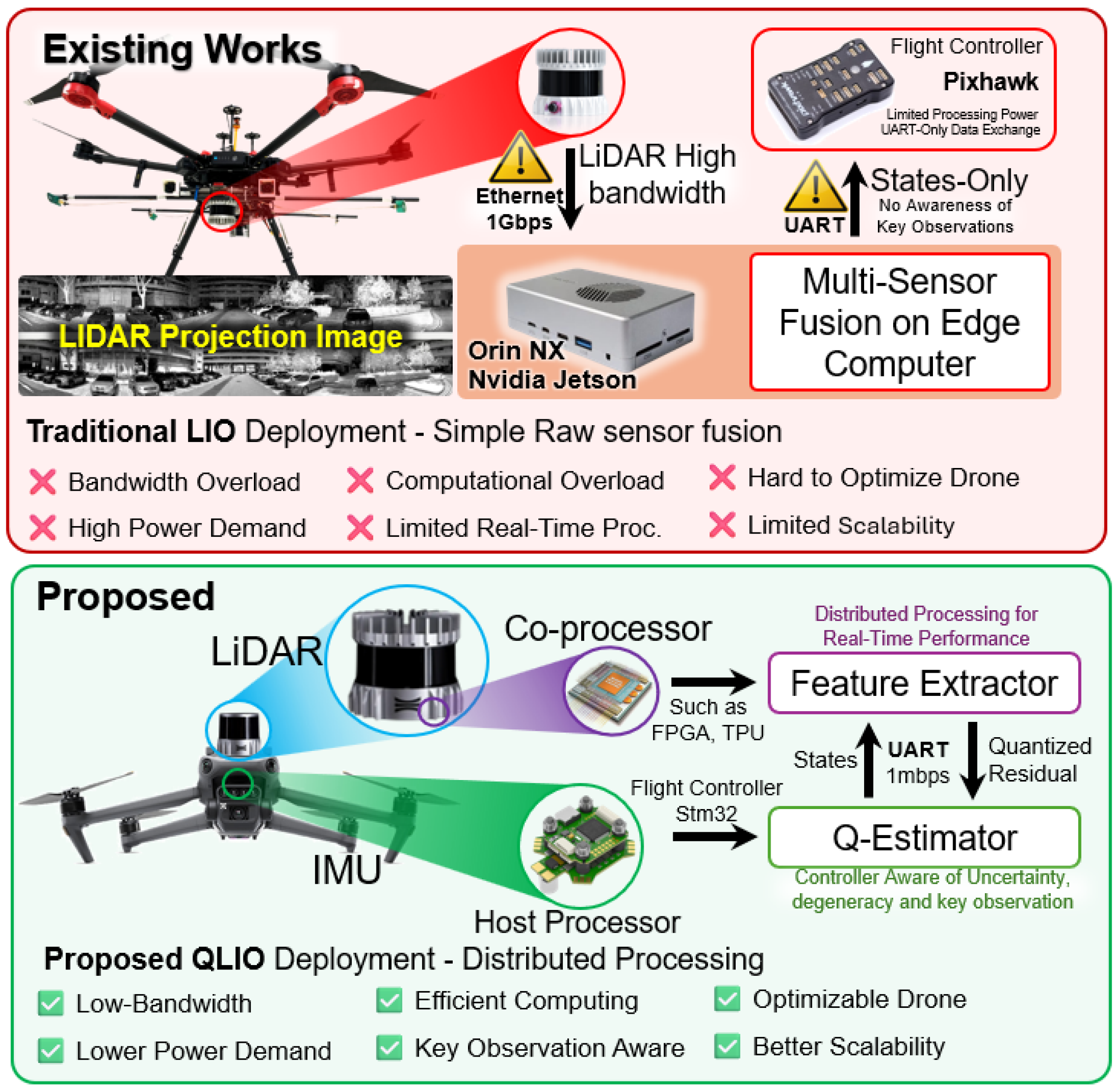
Figure 1: Comparison of Traditional LIO deployment [33, 34, 35] vs. Proposed QLIO: Enhancing Efficiency with Distributed Processing.

While integrating visual perception [19, 36, 37, 32, 38] improves state estimation, it increases computational complexity. The cloud-based LiDAR localization [39, 40, 41] offloads processing but suffers from latency and network constraints. Efficient compression schemes [42, 43, 44, 45, 46] help address bandwidth limitations, yet balancing compression efficiency and data fidelity remains challenging. Meanwhile, advances in SoC architectures [47] and distributed processing frameworks [48] are shifting the research focus to edge computing, optimizing real-time compression, data transmission, and localized processing under strict SWaP constraints.

SoC and distributed processing [47, 48, 49] have proven effective for 2D visual pipelines. However, deploying such a solution to 3D LIO [50, 51, 52] in real-world systems remains challenging due to the trade-off between SWaP and robustness. Robust algorithms require substantial processing power [53], yet practical platforms, such as UAVs and humanoids, must remain lightweight and efficient. This trade-off limits scalability, demanding a rethink of LIO architectures for adaptive processing and efficiency.

To bridge this gap, we propose QLIO, a multi-processor distributed quantized LIO framework tailored for edge devices. Unlike prior work such as Quantized Visual-Inertial Odometry (QVIO) [48], which applies quantization-based estimation to visual features, QLIO introduces LiDAR-specific optimizations that enhance efficiency while maintaining localization accuracy. Our method employs structured point-to-plane residual compression and rQ-vector-based adaptive resampling to reduce computational load and bandwidth consumption without compromising geometric integrity. Our contribution can be summarized as follows.

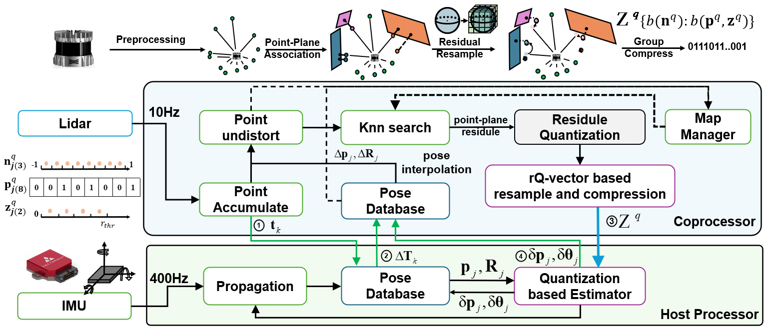
Figure 2: QLIO system architecture with a dual-processor setup. The coprocessor handles LiDAR preprocessing, residual quantization, and compression, while the host processor performs IMU propagation and quantized state estimation, optimizing efficiency for real-time localization.

• Distributed Multi-Processor LIO Architecture: We propose QLIO, a distributed LiDAR-Inertial Odometry framework, leveraging a co-processor for LiDAR preprocessing and a host processor for state estimation. This reduces computational load and bandwidth usage, specifically tailored for LiDAR data.

• Quantized MAP Estimation for LIO: We introduce a multi-bit quantized Maximum A Posteriori (QMAP) estimator for LIO, optimizing 3D LiDAR residuals, reducing data transmission while preserving localization accuracy.

• rQ-Vector-Based Adaptive Resampling and Compression: We present an rQ-vector-based resampling and compression technique, focusing on LiDAR’s 3D geometric structure to improve data efficiency and minimize computational redundancy.

• Open-Source LIO Framework with Real-World Validation: Our open-source QLIO framework is validated on real-world datasets, demonstrating significant bandwidth reduction (14.1×) while maintaining high localization accuracy, making it ideal for SWaP-constrained systems.

II Related Works

To reduce the computational load of the state estimation, LiDAR-SLAM systems [54, 55, 56, 57, 58, 59, 60, 21, 3, 24, 7, 61, 62] often utilize the structural characteristics to quantize the point cloud measurements through feature extraction[63, 64] or voxel downsampling[5, 6]. In subsequent work, downsampling based on an octree structure was proposed [65], as well as adaptive downsampling methods [11] to improve performance in degradation scenarios. Y.C et al. proposed a loop-closure BTC descriptor [66], which obtains a lightweight representation by using binary height description.

Quantized state estimation, though underexplored, has a foundation in observation quantization. The field originated from the SOI-KF framework [39], which introduced 1-bit residual sign discrimination to balance information retention and efficiency. Later advancements extended quantization theory to distributed architectures through multi-bit MAP estimation and IQEKF variants [67, 41, 40]. QVIO [48] further developed this by integrating dual quantization strategies: zQVIO for multi-bit observation quantization and rQVIO for 1-bit residual quantization, achieving millimeter precision with minimal bandwidth. While effective for VIO, QVIO’s 2D pixel-based quantization does not generalize to LIO, which depends on 3D point-cloud geometry. Addressing this gap, QLIO employs structured point-to-plane residual quantization and adaptive rQ-vector grouping for efficient LiDAR data compression while preserving geometric consistency. This innovation bridges quantization theory to LIO, ensuring accurate and bandwidth-efficient processing.

III Quantized LiDAR-Inertial-Odometry

Our framework inherits architectural principles from FastLIO2 [5] and QVIO [48], assuming fixed and pre-calibrated LiDAR-IMU extrinsic parameters excluded from the optimization manifold. The system maintains the core state vector defined in FastLIO2:

$$\mathbf{{x}}\triangleq\left[{\mathop{{}^{G}{\mathbf{R}}_{I}^{T}}},{\mathop{{}^{G}{\mathbf{p}}_{I}^{T}}},{\mathop{{}^{G}{\mathbf{v}}_{I}^{T}}},\mathbf{\mathit{\mathbf{b}}}_{\omega}^{T},\mathbf{\mathit{\mathbf{b}}}_{a}^{T},{\mathop{{}^{G}{\mathbf{g}}_{I}^{T}}}\right]^{T}\in\mathcal{M}$$ (1)

$$\mathbf{u}\triangleq\left[\omega_{m}^{T}\quad\mathbf{a}_{m}^{T}\right]^{T},\mathbf{w}\triangleq\left[\mathbf{n}_{\omega}^{T}\quad\mathbf{n}_{\mathrm{a}}^{T}\quad\mathbf{n}_{\mathrm{b}\omega}^{T}\quad\mathbf{n}_{\mathrm{ba}}^{T}\right]^{T}$$ (2)

$$\mathbf{x}_{i+1}=\mathbf{x}_{i}\boxplus\left(\Delta t\mathbf{f}\left(\mathbf{x}_{i},\mathbf{u}_{i},\mathbf{w}_{i}\right)\right)$$ (3)

$\mathbf{R}$, $\mathbf{p}$, and $\mathbf{v}$ represent rotation, translation, and velocity, respectively. $\mathit{\mathbf{b}}_{a}$ and ${\mathbf{b}}_{\omega}$ are acceleration biases and the angular velocity of the IMU. $\mathbf{g}$ denote the gravity and $\mathbf{w}$ and $\mathbf{u}$ denote IMU measurement noise and control input. Global frame ${}^{G}(\text{·})$ represents the World-fixed reference frame initialized at system startup. Body frame ${}^{I}(\text{·})$ rigidly attached to IMU with origin at its measurement center, establishing the inertial reference for kinematic computations and LiDAR frame ${}^{L}(\text{·})$ defined by LiDAR’s optical center, where raw point clouds are initially captured in this right-handed Cartesian system.

III-A System Overivew

Our system architecture comprises two synchronized components as illustrated in Figure 2.

$$\begin{split}\mathbf{x}_{i+1}=\mathbf{x}_{i}\boxplus\left(\Delta t\mathbf{f}\left(\widehat{\mathbf{x}}_{i},\mathbf{u}_{i},\mathbf{0}\right)\right),\widehat{\mathbf{x}}_{0}=\overline{\mathbf{x}}_{k-1},\\ \widehat{\mathbf{P}}_{i+1}=\mathbf{F}_{\mathbf{x}_{i}}\widehat{\mathbf{P}}_{i}\mathbf{F}_{\mathbf{x}_{i}}^{T}+\mathbf{F}_{\mathbf{w}_{i}}\mathbf{Q}_{i}\mathbf{F}_{\mathbf{w}_{i}}^{T};\widehat{\mathbf{P}}_{0}=\overline{\mathbf{P}}_{k-1}\end{split}$$ (4)

The host processor performs IMU integration and pose updates (Equation 4), while a dedicated co-processor efficiently handles point cloud processing, including nearest neighbor search and residual computation. Unlike Visual-Inertial Odometry (VIO) systems that rely on image-based feature tracking and quantized pixel measurements [48], our method is tailored for LiDAR-Inertial Odometry (LIO), leveraging structured point-to-plane residual quantization to compress geometric information efficiently. By integrating a quantization-aware four-stage pipeline, our architecture minimizes bandwidth and computational costs while maintaining precise inter-processor synchronization.
1. Upon LiDAR scan arrival at timestamp $\mathbf{t}_{k}$, coprocessor sent the pose request with the timestamp $\mathbf{t}_{k}$ to the host-processor.
2. The host-processor responds with the relative pose transform $\Delta\mathbf{T}_{k}=\left(\Delta\mathbf{p}_{k},\Delta{\mathbf{R}}_{k}\right)$ obtained by the short term IMU integration from $\mathbf{t}_{k-1}$ to $\mathbf{t}_{k}$. Then the coprocessor downsample and undistorted the points using the relative pose interpolation and transform points to the global coordinate system:

$$\begin{split}{}^{L}\mathbf{p}_{j}&={{}^{L}\mathbf{T}_{I}}\Delta\mathbf{T}_{j}{{}^{I}\mathbf{T}_{L}}\mathbf{p}_{j}\\ {}^{G}\mathbf{p}_{j}&=\Delta\mathbf{T}_{k}\mathbf{T}_{k-1}{{}^{I}\mathbf{T}_{L}}{{}^{L}\mathbf{p}_{j}}\end{split}$$ (5)

where $\Delta\mathbf{T}_{j}=\left(\Delta\mathbf{p}_{j},\Delta{\mathbf{p}_{j}}_{ori}\right)$ respected to the LiDAR relative pose from the ${{\mathbf{p}}_{j}}_{ori}$ arrived time $\mathbf{t}_{j}$ to the end of the scan $\mathbf{t}_{k}$. Then using the ${}^{G}\mathbf{p}_{j}$ perform knn search based on map manager, finding the nearest five points. If the they can fit an plane, we will find the associations between points and plane, as well as the residual measurements $\mathbf{z}_{i}$ in [5]:

$$\mathbf{z}_{i}=\mathbf{u}_{i}^{T}\left({}^{G}\mathbf{p}_{i}-{}^{G}\mathbf{m}_{i}\right)=\left\|\mathbf{n}_{i}\right\|,\quad\mathbf{n}_{i}=d_{i}\cdot\frac{\mathbf{u}_{i}^{T}}{\left\|\mathbf{u}_{i}^{T}\right\|}$$ (6)

$$0=\mathbf{h}_{i}\left(\mathbf{x}_{k},{}^{L}\mathbf{p}_{i}+{}^{L}\mathbf{n}_{i}\right)$$ (7)

$$\mathbf{z}_{i}+\mathbf{h}_{i}(\mathbf{x}_{k}-\hat{\mathbf{x}}_{k})=-\mathbf{v}_{i}\sim\mathcal{N}\left(0,\mathbf{R}_{i}\right)$$ (8)

where ${\mathbf{v}_{i}}$ and ${\mathbf{R}_{i}}$ denote the measurment noise and covariance matrix. Residual vector $\mathbf{n}$ is obtained by projecting the displacement vector ($\mathbf{p}_{i}-\mathbf{m}_{i}$) onto the normal vector $\mathbf{u}_{i}^{T}$ of the associated plane.
3.Once point-plane association is established, the overall state estimation problem will solely depend on the associated points and residual vectors. We can use $s$ bits quantize them with $\mathbf{f}_{\mathbf{\mathit{p}}_{(s)}}^{\mathbf{\mathit{q}}}$, $\mathbf{f}_{\mathbf{\mathit{z}}_{(s)}}^{\mathbf{\mathit{q}}}$, $\mathbf{f}_{\mathbf{\mathit{n}}_{(s)}}^{\mathbf{\mathit{q}}}$ and perform resampling(Section III-B):

$$\mathbf{z}_{i}^{q} =\mathbf{b}\left(\mathbf{z}_{i}\right)=\mathbf{f}_{\mathbf{\mathit{z}}{(s)}}^{\mathbf{\mathit{q}}}\left(\mathbf{z}_{i}\right)$$ (9)

$${{{}^{L}}}\mathbf{p}_{\mathbf{\mathit{i}}}^{\mathbf{\mathit{q}}} =\mathbf{f}_{\mathbf{\mathit{p}}{(s)}}^{\mathbf{\mathit{q}}}\left({}^{L}\mathbf{p}_{\mathbf{\mathit{i}}}\right),{{{}^{G}}}\mathbf{n}_{\mathbf{\mathit{i}}}^{\mathbf{\mathit{q}}}=\mathbf{f}_{\mathbf{\mathit{n}}{(s)}}^{\mathbf{\mathit{q}}}\left({}^{G}\mathbf{n}_{\mathbf{\mathit{i}}}\right)$$

and then zip the all quantization result ${\mathbf{z}^{q},\mathbf{p}^{\mathbf{\mathit{q}}},\mathbf{n}^{\mathbf{\mathit{q}}}}$ to a group, $\mathcal{Z}^{q}$, and compressed to the bitstream, transmitting them to the host processor.
4.The host processor performs a quantization-based estimator (Section III-C) and updates the pose to the database.

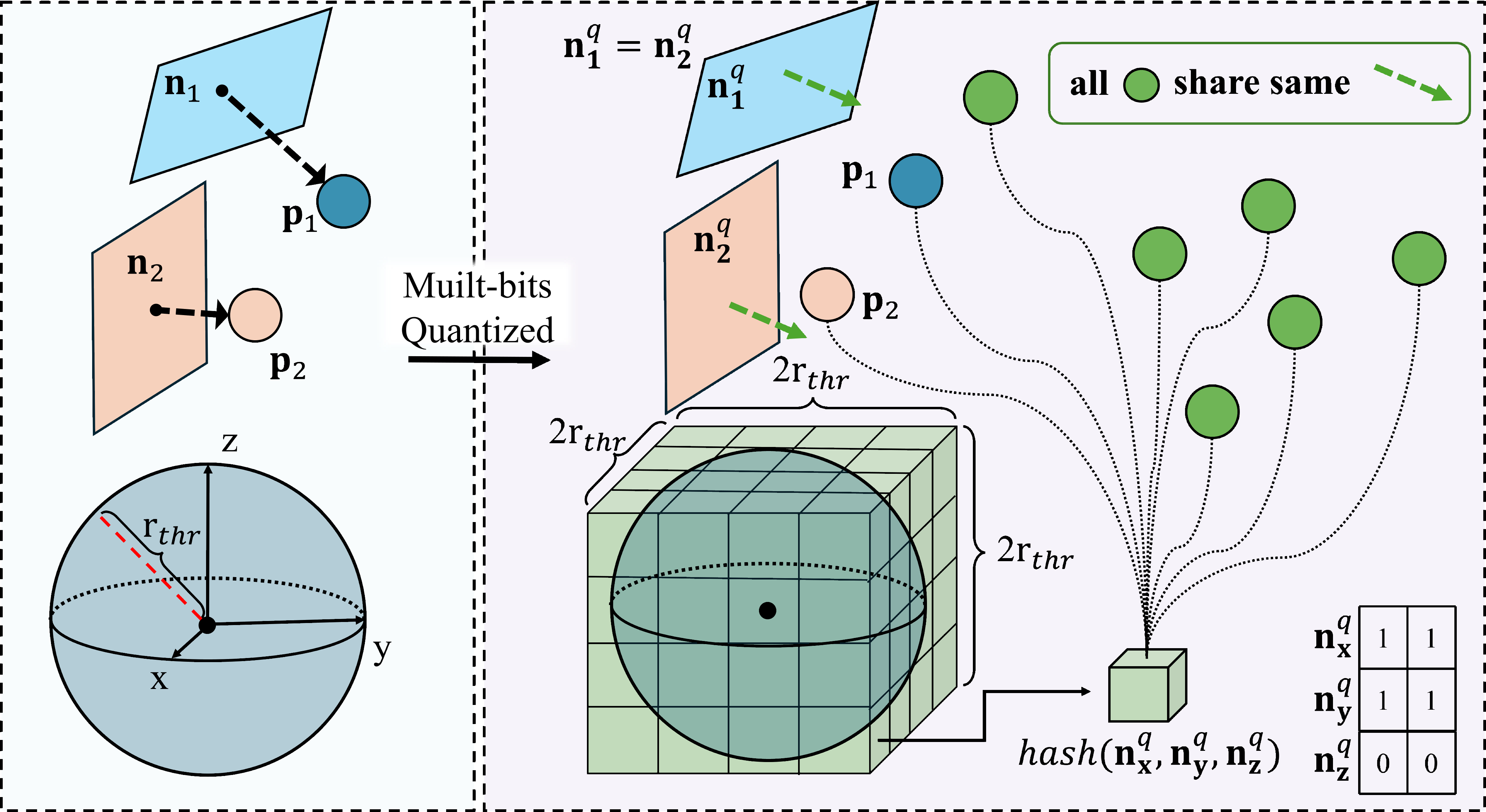
Figure 3: The residual vector space is quantized into a voxel space based on INT-2 quantization. 3D points with the same quantized residuals are grouped into the same hash index. Additionally, the point clouds can be compressed together according to the hash index.

III-B rQ-vector based Resampling and Group Compression

Although point cloud observations have undergone preliminary filtering through voxel downsampling and point-plane association, the remaining points and residual vectors (28 bytes per measurement based on Float32) remain computationally intensive for direct transmission, consuming substantial communication bandwidth. As shown in figure 3, we propose a quantization-based resampling approach that leverages quantized residual vector to construct hash indices and group the points, then adaptive downsample the points those shared with same rQ-vector. If we assume residual $\mathbf{z}=\left\|\mathbf{n}_{i}\right\|<{r}_{thr}$ , the quantization discretizes residual vectors by allocating $s$ bits per axis, creating $2^{s}$ intervals in each dimension that voxelize the normal vector space. This produces $2^{3s}$ unique space cells $\mathcal{C}_{k}$ where $k\in[1,2^{3s}]$, each corresponding to a specific rQ-vector range. For any observed point $\mathbf{p}_{i}$ with original residual vector $\mathbf{n}_{i}$, the quantization process $\mathbf{f}_{\mathbf{\mathit{p}}(s)}^{\mathbf{\mathit{q}}}$ will generate a 3$s$-bit hash key. All points sharing identical $\mathbf{n}^{q}$ are aggregated into the same hash bucket $\mathcal{H}_{k}$, where the bucket index $k$ can computed by hash function:

$$\mathbf{p}_{\mathbf{\mathit{i}}}^{\mathbf{\mathit{q}}}\in\mathcal{H}_{k},k=hash(\mathbf{n}_{\mathbf{\mathit{i}}}^{\mathbf{\mathit{q}}})$$ (10)

This spatial hashing ensures that the points with similar residuals are clustered into identical buckets. We then perform an adaptive 3D downsampling process to each buckets, where downsample size ${ds}_{k}$ can calculate as follows:

$${ds}_{k}={ds}_{0}+\alpha\sum_{i=1}^{n_{k}}\frac{1}{n_{k}}\left\|{\mathbf{\mathbf{p}}_{i}}\right\|$$ (11)

where ${ds}_{0}$ is the cloud preprocessing downsampling parameter and $\alpha$ is the distance penalty coefficient derived from the average Euclidean distance of the points within the same bucket.

Additionally, the filtered points and their corresponding residuals can subsequently be grouped based on rQ-vectors, employing a group encoding scheme with shared header structures to reduce transmission bandwidth. And the groups $\mathcal{Z}^{q}$ can then be constructed as:

$$\begin{split}\mathcal{Z}^{q}&=\left\{b(^{1}\mathbf{n}^{\mathbf{\mathit{q}}}_{k}):b({{}^{1}\mathbf{z}^{q}_{k}},{{}^{1}\mathbf{p}^{\mathbf{\mathit{q}}}_{k}}),b({{}^{2}\mathbf{z}^{q}_{k}},{{}^{2}\mathbf{p}^{\mathbf{\mathit{q}}}_{k}}),b({{}^{3}\mathbf{z}^{q}_{k}},{{}^{3}\mathbf{p}^{\mathbf{\mathit{q}}}_{k}}),...\right\},\\ &\left\{b({{}^{2}\mathbf{n}^{\mathbf{\mathit{q}}}_{k+1}}):b(^{1}{\mathbf{z}^{q}_{k+1}},{{}^{1}\mathbf{p}^{\mathbf{\mathit{q}}}_{k+1}}),b({{}^{2}\mathbf{z}^{q}_{k+1}},{{}^{2}\mathbf{p}^{\mathbf{\mathit{q}}}_{k+1}}),...\right\}...\end{split}$$ (12)

where $b(\text{·})$ denotes the multi-bit binary quantization.

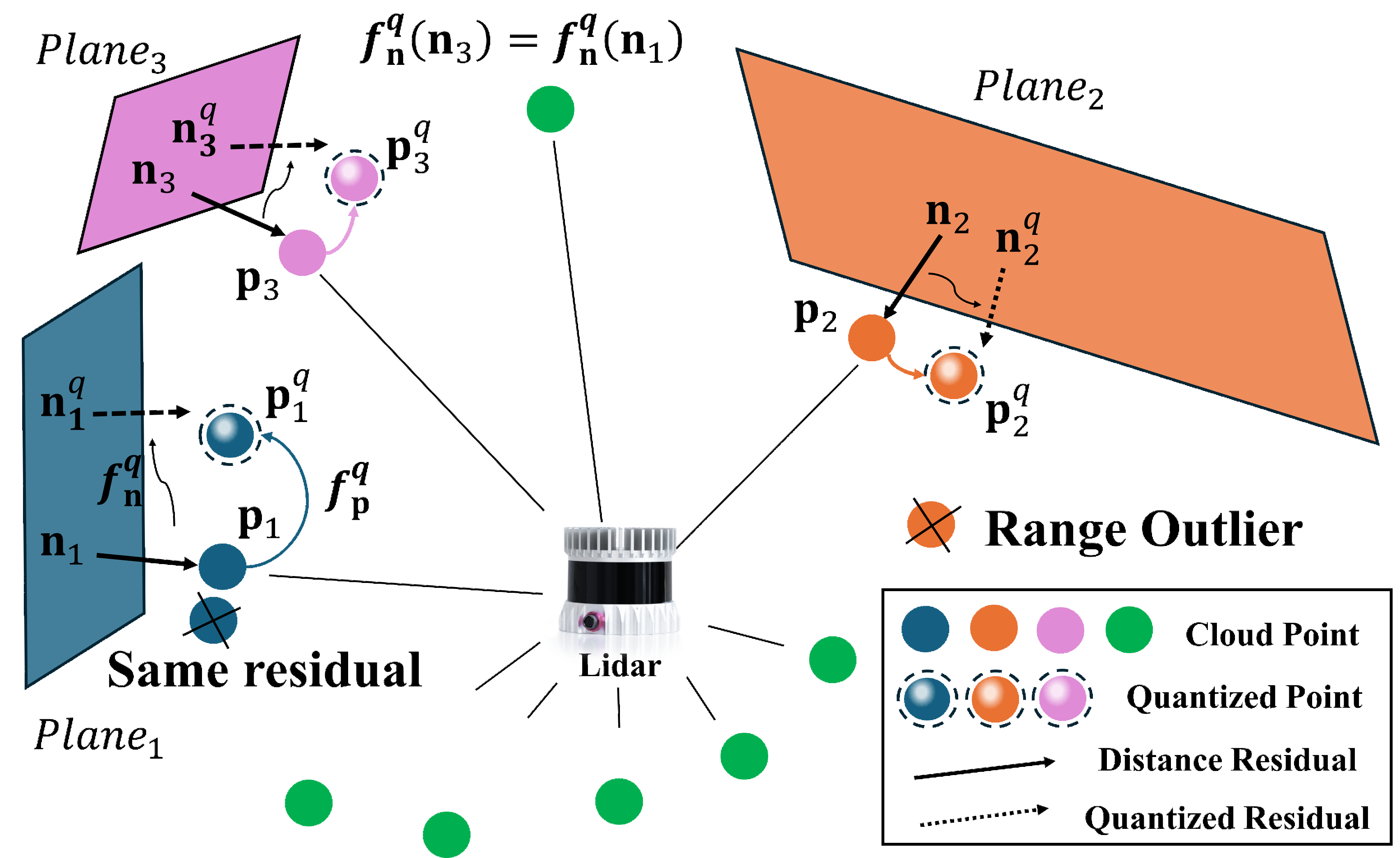
Figure 4: Quantization of the points and their association point-plane residuals.

III-C Quantization-based Estimation

The quantization-based estimation problem can formulate as a MAP problem [40][48]:

$$\arg\max p\left(\mathbf{x}|\mathbf{\mathbf{b}}\left(\mathbf{z}\right)\right)$$ (13)

$$= p\left(\mathbf{x}\right)\prod_{i=1}^{m}p\left(\mathbf{\mathbf{b}}\left(\mathbf{z}_{i}\right)|\mathbf{\mathbf{x}}_{i}\right)$$

$$= p\left(\mathbf{x}\right)\prod_{i=1}^{m}p\left(\mathbf{\mathbf{b}}(\mathbf{z}_{i})\in\left[\mathbf{z}^{0}_{i},\mathbf{z}^{1}_{i}\right]|\mathbf{\mathbf{x}}_{i}\right)$$

The original measurements of the quantized observation residuals $\mathbf{z}^{q}$ should fall within the quantization interval between $\mathbf{z}^{0}$ and $\mathbf{z}^{1}$. Using Equation 8 and $Q$ fuction to :

$$\begin{split}p\left(\mathbf{\mathbf{b}}(\mathbf{z})|\mathbf{x}\right)&=\mathbf{Pr}\left\{\mathbf{z}^{0}<-h\left(\mathbf{x}-\hat{\mathbf{x}}\right)-\mathbf{v}<\mathbf{z}^{1}\middle|\mathbf{x}\right\}\\ &=\mathbf{Pr}\left\{\frac{\mathbf{z}^{0}}{\sigma}<\frac{-h\left(\mathbf{x}-\hat{\mathbf{x}}\right)-\mathbf{v}}{\sigma}<\frac{\mathbf{z}^{1}}{\sigma}\,\middle|\,\mathbf{x}\right\}\\ &=Q\left(\mathbf{\mathcal{X}}^{1}\right)-Q\left(\mathbf{\mathcal{X}}^{0}\right)\end{split}$$ (14)

$$\mathbf{\mathcal{X}}^{0}=\frac{-\mathbf{z}^{0}-h\left(\mathbf{\mathbf{x}}-\hat{\mathbf{\mathbf{x}}}\right)}{\sigma},\textrm{ }\mathbf{\mathcal{X}}^{1}=\frac{-\mathbf{z}^{1}-h\left(\mathbf{\mathbf{x}}-\hat{\mathbf{\mathbf{x}}}\right)}{\sigma}$$ (15)

where $Q(\mathbf{\mathbf{x}})$ is the Gaussian tail probability and $\sigma$ is the scalar of noise standard deviation that normalizes the measurement noise. The MAP problem(Equation 13) is then equivalent to minimizing the following cost function:

$$\begin{split}\mathcal{L\left(\mathbf{x}\right)}&=\left\|\mathbf{x}_{k}\boxminus\hat{\mathbf{x}}_{k}\right\|_{\mathbf{P}_{k}}^{2}+\sum_{i=1}^{m}2ln\left(Q\left(\mathbf{\mathcal{X}}^{1}_{i}\right)-Q\left(\mathbf{\mathcal{X}}^{0}_{i}\right)\right)\\ &=\left\|\mathbf{x}_{k}\boxminus\hat{\mathbf{x}}_{k}\right\|_{\mathbf{P}_{k}}^{2}+\sum_{i=1}^{m}\left\|\mathbf{H}_{i}^{{}^{\prime}}\tilde{\mathbf{x}}+z_{i}^{\prime}\right\|_{\mathbf{R}^{{}^{\prime}}_{k}}^{2}\end{split}$$ (16)

By performing Taylor expansion on Equation 16 and the assumption of quantized measurement-based posterior PDFs will still be close to bell-shaped Gaussian PDFs[41, 40] the above equation can be solved using Kalman filtering[5, 48]:

$$\mathbf{K} =\left({\mathbf{H^{{}^{\prime}}}}^{T}\mathbf{R^{{}^{\prime}}}\mathbf{H^{{}^{\prime}}}+\mathbf{P}^{-1}\right)\mathbf{{H^{{}^{\prime}}}^{T}}\mathbf{{R}^{{}^{\prime}}}^{-1},$$ (17)

$$\overline{\mathbf{x}}_{k} =\hat{\mathbf{x}}_{k}\boxplus\left(-\mathbf{K}\mathbf{z}^{{}^{\prime}}_{k}-\left(\mathbf{I}-\mathbf{K}\mathbf{H^{{}^{\prime}}}\right)\left(\mathbf{J^{{}^{\prime}}}^{-1}\right)\tilde{\mathbf{x}}_{k}\right)$$

Unlike the iterative approach [40], our method is executed in a single pass, eliminating the need for multiple iterations. For further technical details, we refer the reader to the relevant works [41, 48].

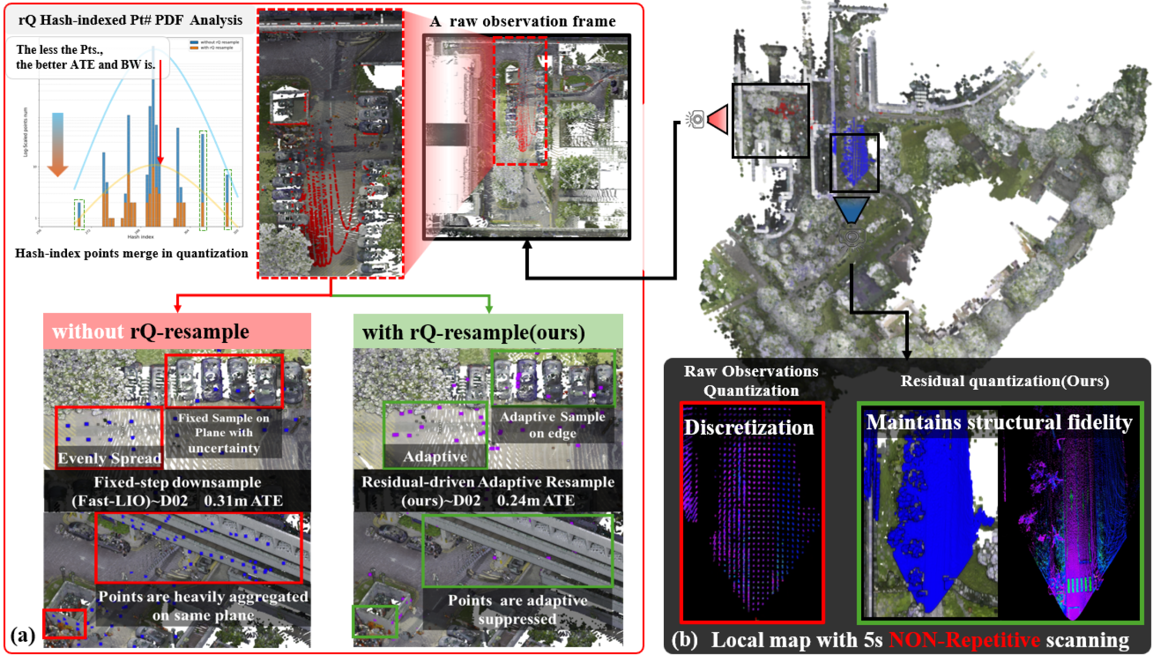
Figure 5: The test result on MCD-NTU dataset. (a) Conventional methods exhibit uniform planar point distributions, while our rQ-resample strategy preserves residual coherence, achieving lower ATE with fewer points. (b) Standard INT8 compression to the raw observation (left) induces discrete local map errors and causes point-plane association failure, whereas residual-aware quantization maintains structural fidelity.

IV Experimental Results

IV-A Quantization Precision Analysis

We adopt a simple and efficient fixed-point quantization for the LiDAR point $\mathbf{p}$, the residual vector $\mathbf{n}$ and the meansurment ${\mathbf{z}}$, which maintains a static codebook configuration. We use $(-{r}_{max},{r}_{max})$ to represent the maximum quantization range of the LiDAR point (e.g. ${r}_{max}$=200m) and filter out the residual norm greater than the threshold ${r}_{thr}$ (e.g. 0.04 cm), meaning the residual space is truncated into a spherical space (see figure 3). Let ${l}_{p}$, ${l}_{n}$ and ${l}_{z}$ as the quantization number of bits, fixed-point multi-bit $\mathbf{p}^{\mathbf{\mathit{q}}}$, $\mathbf{n}^{\mathbf{\mathit{q}}}$, ${\mathbf{z}^{q}}$ and the required bits number with out rQ $N$ can represent as:

$$\mathbf{p}^{\mathbf{\mathit{q}}} =\mathbf{f}_{{p}}^{\mathbf{\mathit{q}}}\left(\mathbf{p}\right)=(p_{1}^{q},p_{2}^{q},p_{3}^{q}),\ \mathbf{n}^{\mathbf{\mathit{q}}}=\mathbf{f}_{{n}}^{\mathbf{\mathit{q}}}\left(\mathbf{n}\right)=(n_{1}^{q},n_{2}^{q},n_{3}^{q})$$ (18)

$$p_{j}^{q} =\left\lfloor\dfrac{p_{j}+r_{max}}{2^{(1-l_{p})}r_{max}}\right\rfloor\cdot 2^{(1-l_{p})}r_{max}-r_{max}+2^{(-l_{p})}r_{max}$$

$$n_{j}^{q} =\left\lfloor\dfrac{n_{j}+r_{thr}}{2^{(1-l_{n})}r_{thr}}\right\rfloor\cdot 2^{(1-l_{n})}r_{thr}-r_{thr}+2^{(-l_{n})}r_{thr}$$

$$\mathbf{z}^{q} =\left\lfloor\dfrac{\mathbf{z}}{2^{(-l_{\mathbf{\mathit{z}}})}{r}_{thr}}\right\rfloor\cdot 2^{(-l_{\mathbf{\mathit{z}}})}{r}_{thr}+2^{(-l_{\mathbf{\mathit{z}}}-1)}{r}_{thr}$$

$$N =3l_{\mathbf{\mathit{p}}}+3l_{\mathbf{\mathit{n}}}+l_{\mathbf{\mathit{z}}},j=1,2,3.$$

where $\left\lfloor\dfrac{p_{j}+r_{max}}{2^{(1-l_{p})}r_{max}}\right\rfloor$ , $\left\lfloor\dfrac{n_{j}+r_{thr}}{2^{(1-l_{n})}r_{thr}}\right\rfloor$, $\left\lfloor\dfrac{\mathbf{z}}{2^{(-l_{\mathbf{\mathit{z}}})}{r}_{thr}}\right\rfloor$ can then compressed to the binary bit stream based on rQ-vector grouping compressed strategy Equation 12.

IV-B Real World Experiment

We evaluate the proposed QLIO on the MCD-NTU dataset[35]. The MCD-NTU dataset was collected using an ATV within the NTU campus with a solid-state hybrid LiDAR (Livox-Mid70, Mid), a mechanical LiDAR (Ouster128, OS) and an external IMU sensor(VN100), including 6 sequnces. Our system is built based on FastLIO[5]. We first conduct a comparative evaluation between FastLIO and our residual-quantized (rQ) vector-based resampling strategy (rQrs) employing fixed hash hierarchy levels ($l_{n}=3$, equivalent to 512 hash buckets). The “X” means failed below and the average absolute trajectory error(ATE) results are shown in the Table I. It can be observed that the accuracy of FastLIO has been significantly improved after the application of rQrs, which is attributed to the resampling of the point observation and the residual, as shown in the Figure 5.

TABLE I: ATE in meters for different methods and sequences.

Method/Seq.	D01	D02	D10	N04	N08	N13
OS	1.48	0.27	2.08	1.59	2.05	1.29
OS-rQrs	1.28	0.23	1.28	1.25	1.62	0.89
Mid	1.09	0.31	1.63	0.85	1.54	1.88
Mid-rQrs	0.91	0.24	1.47	0.49	1.33	2.33
OS-dacro(8)	X	X	X	X	X	X
Mid-INT(8)	X	15.75	X	X	X	X

TABLE II: for different methods and sequences.

Method/Seq.	d-c cost/ms	p.r	bits/mea.	avg.num
OS	0	1	96	15020.65
OS-rQrs	0.59	1	96	566.07
Mid	0	1	96	2799.16
Mid-rQrs	0.23	1	96	248.98
OS-dacro(8)	1868.25	3.98	24.12	16555.97
Mid-INT(8)	0.14	4	24	2665.32

The fixed-step downsampling method arranges observations more regularly(see Figure 5.a “without rQ-resample”), yet induces directional residual concentration bias through its fixed sampling interval, resulting in observation direction imbalance (as per distribution analysis). However, our method resolves this imbalance, achieving measurement uniformity with fewer sampling points while maintaining optimization stability.

In addition, we implemented two conventional point cloud compression methods within our LiDAR-Inertial Odometry (LIO) pipeline to simulate centralized processing with fully compressed observations. To our knowledge, conventional compression methods are rarely tested in such tightly coupled LIO frameworks (most existing evaluations focus on pure LiDAR odometry like LOAM). Specifically, we applied INT8 Quantization and 8-bit Dacro two distinct compression techniques. Both approaches maintained identical post-processing pipelines with the original LIO algorithm where p.r (point cloud compression ratio), d-c (decompress-compress) cost time, and avg.num (average number of points per scan included in state estimation) were measured under varying compression configurations. Surprisingly, both methods exhibited significant performance degradation: INT8 fails because of the precision loss from point value truncation destroyed planar continuity, as shown in Figure 5.b, where original smooth surfaces became discrete grids. This fundamentally disrupted point-to-plane data association. Dacro limits because of the excessive compression/decompression latency (see Table II) caused cumulative IMU integration drift during processing gaps, ultimately compromising state estimation. It should be noted that the observed INT8 quantization-induced plane matching failures may stem from implementation specifics rather than inherent limitations of INT8 quantization. Alternative quantization strategies (e.g., log-scale quantization, variable-bit quantization) could theoretically resolve this, though our exhaustive experiments with these approaches revealed suboptimal performance-all variants required extensive hyperparameter tuning with additional parameters (detailed ablation studies will be documented in the supplementary material) thereby introducing prohibitive complexity in benchmark control. Consequently, we adopted the deterministic min-max INT8 quantization scheme to ensure reproducibility, sacrificing marginal accuracy for experimental stability. Notably, these approaches represent common paradigms for edge-device state estimation and we will then introduce our targeted solution QLIO framework.

TABLE III: ATE meters/rads in different ${l}_{n}$ influences

M/O	${l}_{n}$	D01	D02	D10	N04	N08	N13
OS	1	X	1.21/0.02	X	X	X	X
	2	1.57/0.02	0.25/0.01	1.39/0.03	1.37/0.03	1.54/0.02	0.86/0.04
	3	1.41/0.02	0.29/0.01	1.36/0.03	1.36/0.03	1.82/0.02	0.91/0.04
Mid	1	X	X	X	X	X	X
	2	1.96/0.03	0.56/0.02	1.57/0.02	1.32/0.03	3.89/0.02	X
	3	1.23/0.03	0.29/0.02	1.41/0.02	0.62/0.03	1.40/0.02	X

TABLE IV: ATE in meters/rads for different methods and sequences using differnt ${l}_{z}$.

M/O	${l}_{z}$	D01	D02	D10	N04	N08	N13
OS	1	1.37/0.02	0.24/0.01	1.32/0.03	1.40/0.03	1.76/0.02	0.88/0.04
	2	1.57/0.02	0.24/0.01	1.36/0.03	1.32/0.03	1.58/0.02	0.86/0.04
	3	1.30/0.02	0.25/0.01	1.44/0.03	1.41/0.03	1.90/0.02	0.88/0.04
	4	1.23/0.02	0.24/0.01	1.51/0.03	1.43/0.03	1.79/0.02	0.86/0.04
Mid	1	1.34/0.02	0.43/0.02	1.93/0.02	1.75/0.04	3.09/0.02	X
	2	1.99/0.02	0.29/0.02	1.97/0.02	1.23/0.03	3.28/0.02	X
	3	1.36/0.02	0.32/0.02	1.38/0.02	1.21/0.04	1.56/0.02	X
	4	1.26/0.02	0.31/0.02	1.57/0.02	1.26/0.04	2.46/0.02	X

We first performed comparative ablation studies on residual component quantization bits ${l}_{n}$ versus residual-vector quantization bits ${l}_{z}$ (which may also directly determine the number of the hash bucket) systematically varying each parameter from 1-bit to 3-bit configurations under rQrs. This parametric sweep enabled empirical analysis of accuracy variations under progressive quantization refinement. Our experiments demonstrate that residual vector quantization with ${l}_{n}=1$ consistently induces system failure across both OS and MID platforms, indicating catastrophic sensitivity to insufficient quantization precision. The experimental results of increasing the quantization level reveal distinct platform-dependent characteristics: ${l}_{n}$ demonstrates negligible accuracy variation on OS, whereas MID exhibits consistent precision improvement that correlates with its unique multi-echo radar architecture. As the residual-vector quantization bits ${l}_{z}$ increases, both MID and OS demonstrate minimal variation across all test sequences, with the notable exception of the N13 sequence (as shown in Table V).

On the N13 sequence involving rapid 180° rotations, we observed MID70 divergence. This is attributed to mid70’s single-frame observation mechanism, which differs from Ouster in that it fails to capture a complete spherical point cloud. The incomplete spatial sampling leads to concentrated distributions of residual vectors after low-bit quantization, significantly disrupting original data associations. As we progressively increased quantization bits, system accuracy recovered accordingly. Precision returned to baseline levels when ${l}_{n}=3$. This demonstrates that QLIO requires higher bit allocation under degraded conditions to maintain system stability. However, even when increasing to 4-bit quantization (compared to the original 32-bit float representation), this tradeoff remains worthwhile for devices with stringent communication bandwidth requirements.

TABLE V: ATE result in different combination of ${l}_{z}$ and ${l}_{n}$ using Mid70 in N13.

N13-MID	${l}_{n}=1$	${l}_{n}=2$	${l}_{n}=3$
${l}_{z}=1$	X	X	X
${l}_{z}=2$	X	X	1.31/0.04
${l}_{z}=3$	X	15.54/0.14	1.25/0.04
${l}_{z}=4$	X	4.14/0.06	1.45/0.04

TABLE VI: ATE in meters/rads and the bits/Bytes occupation‌ per measurements for ${l}_{p}$ and sequences.

seq	rQrs	${l}_{p}=3$	${l}_{p}=4$	${l}_{p}=5$	${l}_{p}=6$	${l}_{p}=7$	${l}_{p}=8$	${l}_{p}=9$	${l}_{p}=10$	${l}_{p}=11$	${l}_{p}=12$
D01	w/o	2.95/0.04	2.10/0.04	1.76/0.04	1.62/0.04	1.59/0.04	1.63/0.04	1.61/0.04	1.57/0.04	1.64/0.04	1.68/0.04
	w/	1.98/0.03	1.74/0.03	1.51/0.03	1.52/0.03	1.40/0.03	1.48/0.03	1.46/0.03	1.55/0.03	1.44/0.03	1.51/0.03
D02	w/o	0.33/0.01	0.31/0.01	0.32/0.01	0.31/0.01	0.31/0.01	0.31/0.01	0.31/0.01	0.32/0.01	0.31/0.01	0.31/0.01
	w/	0.24/0.01	0.24/0.01	0.25/0.01	0.26/0.01	0.25/0.01	0.25/0.01	0.25/0.01	0.25/0.01	0.26/0.01	0.26/0.01
D10	w/o	2.74/0.04	2.52/0.04	2.74/0.04	2.76/0.04	2.63/0.04	2.71/0.04	2.69/0.04	2.66/0.04	2.61/0.04	2.58/0.04
	w/	1.18/0.04	1.06/0.04	1.31/0.04	1.27/0.04	1.36/0.04	1.34/0.04	1.30/0.04	1.30/0.04	1.42/0.04	1.30/0.04
N04	w/o	1.60/0.03	1.61/0.03	1.64/0.03	1.64/0.03	1.67/0.03	1.66/0.03	1.70/0.03	1.67/0.03	1.67/0.03	1.65/0.03
	w/	1.21/0.03	1.27/0.03	1.31/0.03	1.41/0.03	1.31/0.03	1.37/0.03	1.41/0.03	1.39/0.03	1.39/0.03	1.40/0.03
N08	w/o	2.62/0.02	2.76/0.02	3.17/0.02	2.91/0.02	3.08/0.02	2.98/0.02	2.98/0.02	3.07/0.02	3.06/0.02	2.89/0.02
	w/	2.07/0.02	1.53/0.02	1.67/0.02	1.85/0.02	1.68/0.02	1.48/0.02	1.54/0.02	1.84/0.02	1.56/0.02	1.75/0.02
N13	w/o	1.41/0.05	1.34/0.05	1.30/0.05	1.30/0.05	1.29/0.05	1.29/0.05	1.29/0.05	1.30/0.05	1.29/0.05	1.29/0.05
	w/	0.89/0.05	0.85/0.05	0.86/0.05	0.87/0.05	0.88/0.05	0.88/0.05	0.89/0.05	0.87/0.05	0.87/0.05	0.87/0.05
avg.b/B	w/o	20/2.50	23/2.87	26/3.25	29/3.62	32/4.00	35/4.37	38/4.75	41/5.12	44/5.50	47/5.87
	w/	5.84/0.73	6.84/0.85	7.84/0.98	8.84/1.10	9.84/1.23	10.84/1.35	11.84/1.48	12.84/1.60	13.84/1.73	14.84/1.85

Based on our prior experiments, we fixed the 3-bit residual vector quantization and 2-bit residual quantization schemes(${l}_{n}=3$, ${l}_{z}=2$) then conducted systematic tests on LiDAR point quantization bits ranging from 3 to 12 bits using Ouster. The corresponding ATE meter/rads results, per-observation bit counts, and byte consumption are detailed inTable VI .The results demonstrate that implementing the rQrs strategy significantly enhances precision while drastically reducing observation counts. This efficiency gain stems from our group compression protocol - points sharing same rQ-vector are packaged together during compression, thereby reducing the cost required for rQ-vector processing.

Figure 6: The total bits per frame in D10 seq.

Surprisingly, significant fluctuations in the quantization bit number did not lead to substantial accuracy loss. Notably, progressive reduction of quantization bits from 12 to 3 bits reveals a precision-bandwidth trade-off: 3-bit quantization achieves minimal measurement overhead (5.84bits per mea.)but also the minimal precision while more bit quantization achieves more precision gain. Crucially, even with 12-bit quantization under rQrs(14.84bits per mea.), total per-frame bandwidth consumption on the MCD-D10 dataset remains below 1.5kB(as shown in Figure 6). This translates to $<$1.2Mbps total bandwidth usage, enabling practical transmission via edge-device-friendly protocols like UART/SPI (typically supporting 1-10Mbps rates).

V Conclusion and Future Work

QLIO redefines LIO deployment on edge devices by integrating multi-processor quantization, adaptive resampling, and extreme bandwidth reduction. It enables real-time LiDAR state estimation on low-power platforms such as drones and humanoid robots. Unlike 2D visual feature quantization methods like QVIO, QLIO introduces structured 3D point-to-plane quantization and a LiDAR-specific MAP-based estimator. The experimental results show a 15.1× per-observation bandwidth reduction while preserving localization accuracy, demonstrating the need for sensor-specific quantization strategies in LiDAR odometry.

However, QLIO currently relies on heuristic quantization parameters, which may limit adaptability to dynamically changing environments. Additionally, its multi-processor architecture, while improving efficiency, introduces hardware dependencies that require careful integration with different computing platforms. Our future research will prioritize the development of an intelligent parameter optimization framework, such as implementing a reinforcement learning-based architecture with multi-head attention mechanisms for adaptive point cloud feature selection. This approach will systematically replace heuristic parameter design in QLIO with bandwidth-aware optimization, particularly improving spectral efficiency in SLAM applications through adaptive data compression strategies based on communication condition monitoring.

References

- [1] S. Yuan, Y. Yang, T. H. Nguyen, T.-M. Nguyen, J. Yang, F. Liu, J. Li, H. Wang, and L. Xie, “Mmaud: A comprehensive multi-modal anti-uav dataset for modern miniature drone threats,” in 2024 IEEE International Conference on Robotics and Automation (ICRA), 2024, pp. 2745–2751.
- [2] T. He, Z. Luo, X. He, W. Xiao, C. Zhang, W. Zhang, K. M. Kitani, C. Liu, and G. Shi, “Omnih2o: Universal and dexterous human-to-humanoid whole-body teleoperation and learning,” Conference on Robot Learning (CoRL), 2024.
- [3] J. Li, S. Yuan, M. Cao, T.-M. Nguyen, K. Cao, and L. Xie, “Hcto: Optimality-aware lidar inertial odometry with hybrid continuous time optimization for compact wearable mapping system,” ISPRS Journal of Photogrammetry and Remote Sensing, vol. 211, pp. 228–243, 2024.
- [4] J. Li, Q. Leng, J. Liu, X. Xu, T. Jin, M. Cao, T.-M. Nguyen, S. Yuan, K. Cao, and L. Xie, “Helmetposer: A helmet-mounted imu dataset for data-driven estimation of human head motion in diverse conditions,” in Proceedings of the IEEE International Conference on Robotics and Automation (ICRA), 2025.
- [5] W. Xu, Y. Cai, D. He, J. Lin, and F. Zhang, “Fast-lio2: Fast direct lidar-inertial odometry,” IEEE Transactions on Robotics, vol. 38, no. 4, pp. 2053–2073, 2022.
- [6] C. Bai, T. Xiao, Y. Chen, H. Wang, F. Zhang, and X. Gao, “Faster-lio: Lightweight tightly coupled lidar-inertial odometry using parallel sparse incremental voxels,” IEEE Robotics and Automation Letters, vol. 7, no. 2, pp. 4861–4868, 2022.
- [7] T.-M. Nguyen, X. Xu, T. Jin, Y. Yang, J. Li, S. Yuan, and L. Xie, “Eigen is all you need: Efficient lidar-inertial continuous-time odometry with internal association,” IEEE Robotics and Automation Letters, vol. 9, no. 6, pp. 5330–5337, 2024.
- [8] T. Shan, B. Englot, D. Meyers, W. Wang, C. Ratti, and D. Rus, “Lio-sam: Tightly-coupled lidar inertial odometry via smoothing and mapping,” in 2020 IEEE/RSJ international conference on intelligent robots and systems (IROS). IEEE, 2020, pp. 5135–5142.
- [9] T.-M. Nguyen, S. Yuan, M. Cao, L. Yang, T. H. Nguyen, and L. Xie, “Miliom: Tightly coupled multi-input lidar-inertia odometry and mapping,” IEEE Robotics and Automation Letters, vol. 6, no. 3, pp. 5573–5580, 2021.
- [10] T. Shan, B. Englot, C. Ratti, and D. Rus, “Lvi-sam: Tightly-coupled lidar-visual-inertial odometry via smoothing and mapping,” in 2021 IEEE international conference on robotics and automation (ICRA). IEEE, 2021, pp. 5692–5698.
- [11] H. Lim, D. Kim, B. Kim, and H. Myung, “Adalio: Robust adaptive lidar-inertial odometry in degenerate indoor environments,” in 2023 20th International Conference on Ubiquitous Robots (UR). IEEE, 2023, pp. 48–53.
- [12] T.-M. Nguyen, D. Duberg, P. Jensfelt, S. Yuan, and L. Xie, “Slict: Multi-input multi-scale surfel-based lidar-inertial continuous-time odometry and mapping,” IEEE Robotics and Automation Letters, vol. 8, no. 4, pp. 2102–2109, 2023.
- [13] I. Vizzo, T. Guadagnino, B. Mersch, L. Wiesmann, J. Behley, and C. Stachniss, “Kiss-icp: In defense of point-to-point icp–simple, accurate, and robust registration if done the right way,” IEEE Robotics and Automation Letters, vol. 8, no. 2, pp. 1029–1036, 2023.
- [14] K. Chen, R. Nemiroff, and B. T. Lopez, “Direct lidar-inertial odometry: Lightweight lio with continuous-time motion correction,” in 2023 IEEE international conference on robotics and automation (ICRA). IEEE, 2023, pp. 3983–3989.
- [15] Z. Chen, Y. Xu, S. Yuan, and L. Xie, “ig-lio: An incremental gicp-based tightly-coupled lidar-inertial odometry,” IEEE Robotics and Automation Letters, vol. 9, no. 2, pp. 1883–1890, 2024.
- [16] X. Ji, S. Yuan, P. Yin, and L. Xie, “Lio-gvm: an accurate, tightly-coupled lidar-inertial odometry with gaussian voxel map,” IEEE Robotics and Automation Letters, vol. 9, no. 3, pp. 2200–2207, 2024.
- [17] Y. Wu, T. Guadagnino, L. Wiesmann, L. Klingbeil, C. Stachniss, and H. Kuhlmann, “Lio-ekf: High frequency lidar-inertial odometry using extended kalman filters,” in 2024 IEEE International Conference on Robotics and Automation (ICRA). IEEE, 2024, pp. 13 741–13 747.
- [18] M. Eisoldt, J. Gaal, T. Wiemann, M. Flottmann, M. Rothmann, M. Tassemeier, and M. Porrmann, “A fully integrated system for hardware-accelerated tsdf slam with lidar sensors (hatsdf slam),” Robotics and Autonomous Systems, vol. 156, p. 104205, 2022.
- [19] J. Lin and F. Zhang, “R 3 live: A robust, real-time, rgb-colored, lidar-inertial-visual tightly-coupled state estimation and mapping package,” in 2022 International Conference on Robotics and Automation (ICRA). IEEE, 2022, pp. 10 672–10 678.
- [20] T. Jin, X. Xu, Y. Yang, S. Yuan, T.-M. Nguyen, J. Li, and L. Xie, “Robust loop closure by textual cues in challenging environments,” IEEE Robotics and Automation Letters, vol. 10, no. 1, pp. 812–819, 2025.
- [21] J. Li, T.-M. Nguyen, S. Yuan, and L. Xie, “Pss-ba: Lidar bundle adjustment with progressive spatial smoothing,” in 2024 IEEE/RSJ International Conference on Intelligent Robots and Systems (IROS), 2024, pp. 1124–1129.
- [22] J. Li, T.-M. Nguyen, M. Cao, S. Yuan, T.-Y. Hung, and L. Xie, “Graph optimality-aware stochastic lidar bundle adjustment with progressive spatial smoothing,” in arXiv preprint arXiv:2410.14565, 2024.
- [23] Y. Ma, J. Xu, S. Yuan, T. Zhi, W. Yu, J. Zhou, and L. Xie, “Mm-lins: a multi-map lidar-inertial system for over-degenerate environments,” IEEE Transactions on Intelligent Vehicles, vol. -, pp. 1–11, 2024.
- [24] P. Yin, H. Cao, T.-M. Nguyen, S. Yuan, S. Zhang, K. Liu, and L. Xie, “Outram: One-shot global localization via triangulated scene graph and global outlier pruning,” in 2024 IEEE International Conference on Robotics and Automation (ICRA). IEEE, 2024, pp. 13 717–13 723.
- [25] C. Zhao, K. Hu, J. Xu, L. Zhao, B. Han, K. Wu, M. Tian, and S. Yuan, “Adaptive-lio: Enhancing robustness and precision through environmental adaptation in lidar inertial odometry,” IEEE Internet of Things Journal, 2024.
- [26] H. Rebecq, T. Horstschäfer, G. Gallego, and D. Scaramuzza, “Evo: A geometric approach to event-based 6-dof parallel tracking and mapping in real time,” IEEE Robotics and Automation Letters, vol. 2, no. 2, pp. 593–600, 2016.
- [27] W. Wang, D. Zhu, X. Wang, Y. Hu, Y. Qiu, C. Wang, Y. Hu, A. Kapoor, and S. Scherer, “Tartanair: A dataset to push the limits of visual slam,” in 2020 IEEE/RSJ International Conference on Intelligent Robots and Systems (IROS). IEEE, 2020, pp. 4909–4916.
- [28] M. Helmberger, K. Morin, B. Berner, N. Kumar, G. Cioffi, and D. Scaramuzza, “The hilti slam challenge dataset,” IEEE Robotics and Automation Letters, vol. 7, no. 3, pp. 7518–7525, 2022.
- [29] A. D. Nair, J. Kindle, P. Levchev, and D. Scaramuzza, “Hilti slam challenge 2023: Benchmarking single+ multi-session slam across sensor constellations in construction,” IEEE Robotics and Automation Letters, 2024.
- [30] C. Wang, J. Yuan, and L. Xie, “Non-iterative slam,” in 2017 18th International Conference on Advanced Robotics (ICAR). IEEE, 2017, pp. 83–90.
- [31] Z. Yang, K. Xu, S. Yuan, and L. Xie, “A fast and light-weight noniterative visual odometry with rgb-d cameras,” Unmanned Systems, vol. 0, no. 0, pp. 1–13, 2024.
- [32] C. Zheng, W. Xu, Z. Zou, T. Hua, C. Yuan, D. He, B. Zhou, Z. Liu, J. Lin, F. Zhu et al., “Fast-livo2: Fast, direct lidar-inertial-visual odometry,” IEEE Transactions on Robotics, 2024.
- [33] T.-M. Nguyen, M. Cao, S. Yuan, Y. Lyu, T. H. Nguyen, and L. Xie, “Viral-fusion: A visual-inertial-ranging-lidar sensor fusion approach,” IEEE Transactions on Robotics, vol. 38, no. 2, pp. 958–977, 2021.
- [34] T.-M. Nguyen, S. Yuan, M. Cao, Y. Lyu, T. H. Nguyen, and L. Xie, “Ntu viral: A visual-inertial-ranging-lidar dataset, from an aerial vehicle viewpoint,” The International Journal of Robotics Research, vol. 41, no. 3, pp. 270–280, 2022.
- [35] T.-M. Nguyen, S. Yuan, T. H. Nguyen, P. Yin, H. Cao, L. Xie, M. Wozniak, P. Jensfelt, M. Thiel, J. Ziegenbein et al., “Mcd: Diverse large-scale multi-campus dataset for robot perception,” in Proceedings of the IEEE/CVF Conference on Computer Vision and Pattern Recognition, 2024, pp. 22 304–22 313.
- [36] K. Xu, Y. Hao, S. Yuan, C. Wang, and L. Xie, “Airvo: An illumination-robust point-line visual odometry,” in 2023 IEEE/RSJ International Conference on Intelligent Robots and Systems (IROS). IEEE, 2023, pp. 3429–3436.
- [37] P. Pfreundschuh, H. Oleynikova, C. Cadena, R. Siegwart, and O. Andersson, “Coin-lio: Complementary intensity-augmented lidar inertial odometry,” in 2024 IEEE International Conference on Robotics and Automation (ICRA). IEEE, 2024, pp. 1730–1737.
- [38] K. Xu, Y. Hao, S. Yuan, C. Wang, and L. Xie, “Airslam: An efficient and illumination-robust point-line visual slam system,” IEEE Transactions on Robotics, 2025.
- [39] A. Ribeiro, G. B. Giannakis, and S. I. Roumeliotis, “Soi-kf: Distributed kalman filtering with low-cost communications using the sign of innovations,” IEEE Transactions on signal processing, vol. 54, no. 12, pp. 4782–4795, 2006.
- [40] N. Trawny, S. I. Roumeliotis, and G. B. Giannakis, “Cooperative multi-robot localization under communication constraints,” in 2009 IEEE international conference on robotics and automation. IEEE, 2009, pp. 4394–4400.
- [41] E. J. Msechu, S. I. Roumeliotis, A. Ribeiro, and G. B. Giannakis, “Decentralized quantized kalman filtering with scalable communication cost,” IEEE Transactions on Signal Processing, vol. 56, no. 8, pp. 3727–3741, 2008.
- [42] R. Schnabel and R. Klein, “Octree-based point-cloud compression.” PBG@ SIGGRAPH, vol. 3, no. 3, 2006.
- [43] F. Galligan, M. Hemmer, O. Stava, F. Zhang, and J. Brettle, “Google/draco: a library for compressing and decompressing 3d geometric meshes and point clouds,” 2018.
- [44] D. Graziosi, O. Nakagami, S. Kuma, A. Zaghetto, T. Suzuki, and A. Tabatabai, “An overview of ongoing point cloud compression standardization activities: Video-based (v-pcc) and geometry-based (g-pcc),” APSIPA Transactions on Signal and Information Processing, vol. 9, p. e13, 2020.
- [45] S. Wang, J. Jiao, P. Cai, and L. Wang, “R-pcc: A baseline for range image-based point cloud compression,” in 2022 International Conference on Robotics and Automation (ICRA). IEEE, 2022, pp. 10 055–10 061.
- [46] J. Wang, D. Ding, Z. Li, X. Feng, C. Cao, and Z. Ma, “Sparse tensor-based multiscale representation for point cloud geometry compression,” IEEE Transactions on Pattern Analysis and Machine Intelligence, vol. 45, no. 7, pp. 9055–9071, 2022.
- [47] D. Jiang, B. Liu, J. Wang, A. Hu, Y. Zhao, M. Bao, Z. Fan, Z. Shen, K. Wang, and C. Wang, “Live demonstration: A reconfigurable, energy-efficient and high-frame-rate ekf-slam accelerator based soc design for autonomous mobile robot applications,” in 2024 IEEE International Symposium on Circuits and Systems (ISCAS). IEEE, 2024, pp. 1–1.
- [48] Y. Peng, C. Chen, and G. Huang, “Quantized visual-inertial odometry,” in 2024 IEEE International Conference on Robotics and Automation (ICRA). IEEE, 2024, pp. 17 954–17 960.
- [49] Z. Huai and G. Huang, “A consistent parallel estimation framework for visual-inertial slam,” IEEE Transactions on Robotics, 2024.
- [50] H. Cai, S. Yuan, X. Li, J. Guo, and J. Liu, “Bev-lio (lc): Bev image assisted lidar-inertial odometry with loop closure,” arXiv preprint arXiv:2502.19242, 2025.
- [51] J. Li, X. Xu, J. Liu, K. Cao, S. Yuan, and L. Xie, “Ua-mpc: Uncertainty-aware model predictive control for motorized lidar odometry,” IEEE Robotics and Automation Letters, 2025.
- [52] J. Li, Z. Liu, X. Xu, J. Liu, S. Yuan, and L. Xie, “Limo-calib: On-site fast lidar-motor calibration for quadruped robot-based panoramic 3d sensing system,” arXiv preprint arXiv:2502.12655, 2025.
- [53] X. Ji, S. Yuan, J. Li, P. Yin, H. Cao, and L. Xie, “Sgba: Semantic gaussian mixture model-based lidar bundle adjustment,” IEEE Robotics and Automation Letters, vol. 9, no. 12, pp. 10 922–10 929, 2024.
- [54] M. Cao, T.-M. Nguyen, S. Yuan, A. Anastasiou, A. Zacharia, S. Papaioannou, P. Kolios, C. G. Panayiotou, M. M. Polycarpou, X. Xu et al., “Cooperative aerial robot inspection challenge: A benchmark for heterogeneous multi-uav planning and lessons learned,” arXiv preprint arXiv:2501.06566, 2025.
- [55] H. Liang, Y. Yang, J. Hu, J. Yang, F. Liu, and S. Yuan, “Unsupervised uav 3d trajectories estimation with sparse point clouds,” in Proceedings of the IEEE International Conference on Acoustics, Speech, and Signal Processing (ICASSP). IEEE, 2025.
- [56] J. Xu, G. Huang, W. Yu, X. Zhang, L. Zhao, R. Li, S. Yuan, and L. Xie, “Selective kalman filter: When and how to fuse multi-sensor information to overcome degeneracy in slam,” in arXiv preprint arXiv:2412.17235, 2024.
- [57] T. Deng, Y. Chen, L. Zhang, J. Yang, S. Yuan, J. Liu, D. Wang, H. Wang, and W. Chen, “Compact 3d gaussian splatting for dense visual slam,” in arXiv preprint arXiv:2403.11247, 2024.
- [58] T.-M. Nguyen, Z. Cao, K. Li, S. Yuan, and L. Xie, “Gptr: Gaussian process trajectory representation for continuous-time motion estimation,” in arXiv preprint arXiv:2410.22931, 2024.
- [59] R. Bai, S. Yuan, H. Guo, P. Yin, W.-Y. Yau, and L. Xie, “Collaborative graph exploration with reduced pose-slam uncertainty via submodular optimization,” in Proceedings of the 2024 IEEE/RSJ International Conference on Intelligent Robots and Systems (IROS). IEEE, 2024.
- [60] W. Yu, J. Xu, C. Zhao, L. Zhao, T.-M. Nguyen, S. Yuan, M. Bai, and L. Xie, “I2ekf-lo: A dual-iteration extended kalman filter based lidar odometry,” in 2024 IEEE/RSJ International Conference on Intelligent Robots and Systems (IROS), 2024, pp. 10 453–10 460.
- [61] T. Ji, S. Yuan, and L. Xie, “Robust rgb-d slam in dynamic environments for autonomous vehicles,” in 2022 17th International Conference on Control, Automation, Robotics and Vision (ICARCV). IEEE, 2022, pp. 665–671.
- [62] T.-M. Nguyen, M. Cao, S. Yuan, Y. Lyu, T. H. Nguyen, and L. Xie, “Liro: Tightly coupled lidar-inertia-ranging odometry,” in 2021 IEEE international conference on robotics and automation (ICRA). IEEE, 2021, pp. 14 484–14 490.
- [63] J. Zhang, S. Singh et al., “Loam: Lidar odometry and mapping in real-time.” in Robotics: Science and systems, vol. 2, no. 9. Berkeley, CA, 2014, pp. 1–9.
- [64] T. Shan and B. Englot, “Lego-loam: Lightweight and ground-optimized lidar odometry and mapping on variable terrain,” in 2018 IEEE/RSJ International Conference on Intelligent Robots and Systems (IROS). IEEE, 2018, pp. 4758–4765.
- [65] Z. Liu, H. Li, C. Yuan, X. Liu, J. Lin, R. Li, C. Zheng, B. Zhou, W. Liu, and F. Zhang, “Voxel-slam: A complete, accurate, and versatile lidar-inertial slam system,” arXiv preprint arXiv:2410.08935, 2024.
- [66] C. Yuan, J. Lin, Z. Liu, H. Wei, X. Hong, and F. Zhang, “Btc: A binary and triangle combined descriptor for 3-d place recognition,” IEEE Transactions on Robotics, vol. 40, pp. 1580–1599, 2024.
- [67] E. D. Nerurkar and S. I. Roumeliotis, “A communication-bandwidth-aware hybrid estimation framework for multi-robot cooperative localization,” in 2013 IEEE/RSJ International Conference on Intelligent Robots and Systems. IEEE, 2013, pp. 1418–1425.