BUFFER-X: Towards Zero-Shot Point Cloud Registration in Diverse Scenes

Abstract

Recent advances in deep learning-based point cloud registration have improved generalization, yet most methods still require retraining or manual parameter tuning for each new environment. In this paper, we identify three key factors limiting generalization: (a) reliance on environment-specific voxel size and search radius, (b) poor out-of-domain robustness of learning-based keypoint detectors, and (c) raw coordinate usage, which exacerbates scale discrepancies. To address these issues, we present a zero-shot registration pipeline called BUFFER-X by (a) adaptively determining voxel size/search radii, (b) using farthest point sampling to bypass learned detectors, and (c) leveraging patch-wise scale normalization for consistent coordinate bounds. In particular, we present a multi-scale patch-based descriptor generation and a hierarchical inlier search across scales to improve robustness in diverse scenes. We also propose a novel generalizability benchmark using 11 datasets that cover various indoor/outdoor scenarios and sensor modalities, demonstrating that BUFFER-X achieves substantial generalization without prior information or manual parameter tuning for the test datasets. Our code is available at https://github.com/MIT-SPARK/BUFFER-X.

1 Introduction

The field of deep learning-based point cloud registration has made steady and remarkable progress, including enhancing feature distinctiveness [2, 4, 5, 6, 16, 49, 32, 15], improving data association strategies [32, 91, 90, 26, 45, 46, 87, 44], and developing more robust pose estimation solvers [67, 33, 79, 94]. Consequently, existing approaches achieve strong performance on test sequences within the same dataset used for training, successfully estimating the relative pose between two partially overlapping point clouds [77, 40, 43, 78, 10, 84].

More recently, there has been growing interest in tackling the generalization of these deep learning-based methods [5, 6, 54, 25, 17], which is the capability of a network to perform well across diverse real-world scenarios. While these approaches have demonstrated excellent generalization performance, in practice, most existing methods still require the user to provide optimal parameters, such as voxel size for downsampling cloud points and search radius for descriptor generation, when dealing with unseen domain datasets. In this paper, we refer to this manual tuning as an oracle. Therefore, it is still desirable to develop zero-shot registration approaches for better usability and practical deployment.

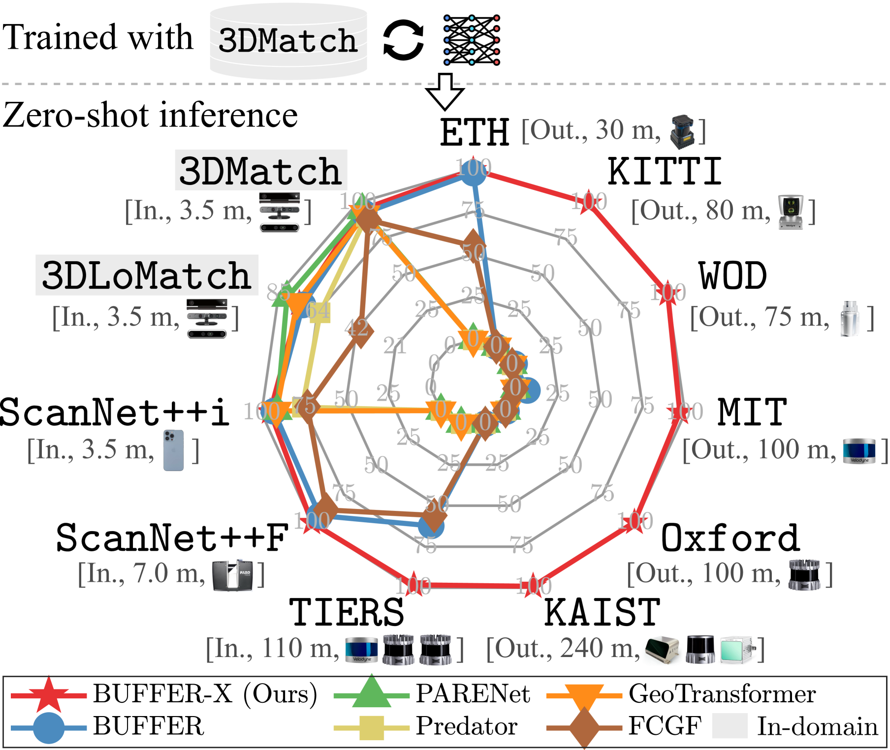
Fig. 1: Sucess rate (unit: %) of zero-shot point cloud registration with state-of-the-art approaches on 11 datasets [28, 88, 34, 32, 81, 60, 61, 69, 71, 56]. Without any prior information or manual parameter tuning for the test datasets, our BUFFER-X shows robust generalization capability across diverse scenes even though the network is only trained on the 3DMatch dataset [88].

Furthermore, despite nearly a decade of research in deep learning-based registration, most studies remain confined to specific scenarios, primarily conducting experiments using omnidirectional LiDAR point clouds for outdoor environments [82, 28] and RGB-D depth clouds for indoor settings [88]. For this reason, domain generalization experiments on LiDAR point clouds in indoors [60] or with different LiDAR scan patterns in outdoor environments [60, 34, 39] are less explored. This underscores the need for a new benchmark that better reflects real-world sensor variations to evaluate generalizability across unseen environments and diverse scanning patterns.

In this context, the main contribution of this paper is addressing two key issues above and propose: a) a zero-shot registration architecture and b) a novel benchmark to help evaluate the generalization capability of deep learning-based registration approaches, as shown in Fig. 1. First, inspired by the remarkable generalization of BUFFER [5] as long as a user manually tunes the voxel size and search radius, we first thoroughly analyze the architectural principles that underpin its generalization. Then, we identify three factors that hinder the zero-shot capabilities of existing methods in Sec. 3. Building on these insights, we introduce a self-adaptive mechanism to determine the optimal voxel size for each test scene and streamline the pipeline of BUFFER, ultimately presenting a robust multi-scale patch-wise approach. We name our approach BUFFER-X to signify that it is an extension of BUFFER.

Second, we establish a comprehensive benchmark that encompasses both indoor and outdoor settings, ensuring that outdoor settings include culturally and geographically diverse locations (e.g., captured in Europe, Asia, and the USA), various environmental scales (ranging from meters to kilometers), and different LiDAR scanning patterns, while indoor settings also incorporate LiDAR-captured data. Subsequently, we demonstrate that our method achieves promising generalization capability without any prior information or manual parameter tuning during the evaluation; see Fig. 1.

In summary, we make three key claims: (i) we thoroughly analyze the limitations of existing approaches and identify the key factors that have hindered zero-shot generalization, (ii) we present an improved approach, named BUFFER-X, that addresses the generalization issues of state-of-the-art methods, and (iii) we introduce a benchmark to evaluate zero-shot generalization performance comprehensively.

2 Related Work

3D point cloud registration, which estimates the relative pose between two partially overlapping point clouds, is a fundamental problem in the fields of robotics and computer vision [7, 83, 18, 13, 37]. Overall, point cloud registration methods are classified into two categories based on whether their performance relies on the availability of an initial guess for registration: a) local registration [11, 66, 55, 36, 57, 72] and b) global registration [27, 24, 78, 94, 10, 76, 77, 43, 40]. Global registration methods can be further classified into two types: a) correspondence-free [62, 12, 10, 52, 23, 19, 65, 50, 31, 51, 93] and b) correspondence-based [27, 78, 94, 24, 38, 87, 44, 86] approaches. In this study, we focus on the latter and particularly place more emphasis on deep learning-based registration methods.

Since Qi et al. [58] demonstrated that learning-based techniques in 2D images can also be applied to 3D point clouds, a wide range of learning-based point cloud registration approaches have been proposed. Building on these advances, novel network architectures with increased capacity have continuously emerged, ranging from MinkUNet [22, 20, 21], cylindrical convolutional network [6, 5, 95], KPConv [32, 70, 8] to Transformers [59, 74, 73, 16].

While these advancements have led to improved registration performance, some of these methods often exhibit limited generalization capability, leading to performance degradation when applied to point clouds captured by different sensor configurations or in unseen environments. To tackle the generalization problem, Ao et al. [6, 3] introduce SpinNet, a patch-based method that normalizes the range of local point coordinates within a fixed-radius neighborhood to $[-1,1]$. This makes us come to realize that patch-wise scale normalization is key to achieving a data-agnostic registration pipeline.

Further, Ao et al. [5] proposed BUFFER to enhance efficiency by combining point-wise feature extraction with patch-wise descriptor generation. However, we found that such learning-based keypoint detectors can hinder robust generalization, as their failure in out-of-domain distributions may trigger a cascading failure in subsequent steps; see Sec. 3.2.3. In addition, despite the high generalizability of BUFFER, we observed that during cross-domain testing, users had to manually specify the optimal voxel size for the test data, which hinders fully zero-shot inference.

Under these circumstances, we revisit the generalization problem in point cloud registration and explore how to achieve zero-shot registration while preserving the key benefits of BUFFER’s scale normalization strategy. In addition, we remove certain modules that hinder robustness and introduce an adaptive mechanism that determines the voxel size and search radii depending on the given cloud points pair. To the best of our knowledge, this is the first approach to evaluate the zero-shot generalization across diverse scenes covering various environments, geographic regions, scales, sensor types, and acquisition setups.

3 Preliminaries

3.1 Problem statement

The goal of point cloud registration is to estimate the relative 3D rotation matrix ${\bm{R}}\in\mathrm{SO}(3)$ and translation vector ${\bm{t}}\in\mathbb{R}^{3}$ between two unordered 3D point clouds $\mathcal{P}$ and $\mathcal{Q}$. To this end, most approaches [32, 41] follow three steps: a) apply voxel sampling $f_{v}({\cdot})$ to the point cloud with voxel size $v$ as preprocessing, b) establish associations (or correspondences) $\mathcal{A}$, and c) estimate ${\bm{R}}$ and ${\bm{t}}$.

Formally, by denoting corresponding points for a correspondence $(i,j)$ in $\mathcal{A}$ as ${\bm{p}}_{i}\in f_{v}({\mathcal{P}})$ and ${\bm{q}}_{j}\in f_{v}({\mathcal{Q}})$, respectively, the objective function used for pose estimation can be defined as:

$$\hat{{\bm{R}}},\hat{{\bm{t}}}=\operatorname*{arg\,min}_{{\bm{R}}\in\mathrm{SO}(3),{\bm{t}}\in\mathbb{R}^{3}}\sum_{(i,j)\in\mathcal{A}}\rho\Big{(}\|{\bm{q}}_{j}-{\bm{R}}{\bm{p}}_{i}-{\bm{t}}\|_{2}\Big{)},$$ (1)

where $\rho(\cdot)$ represents a nonlinear kernel function that mitigates the effect of spurious correspondences in $\mathcal{A}$.

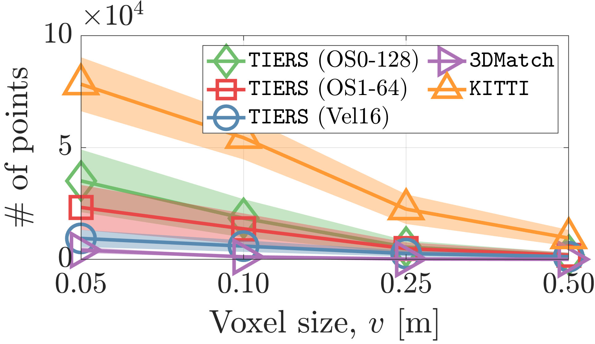
(a)

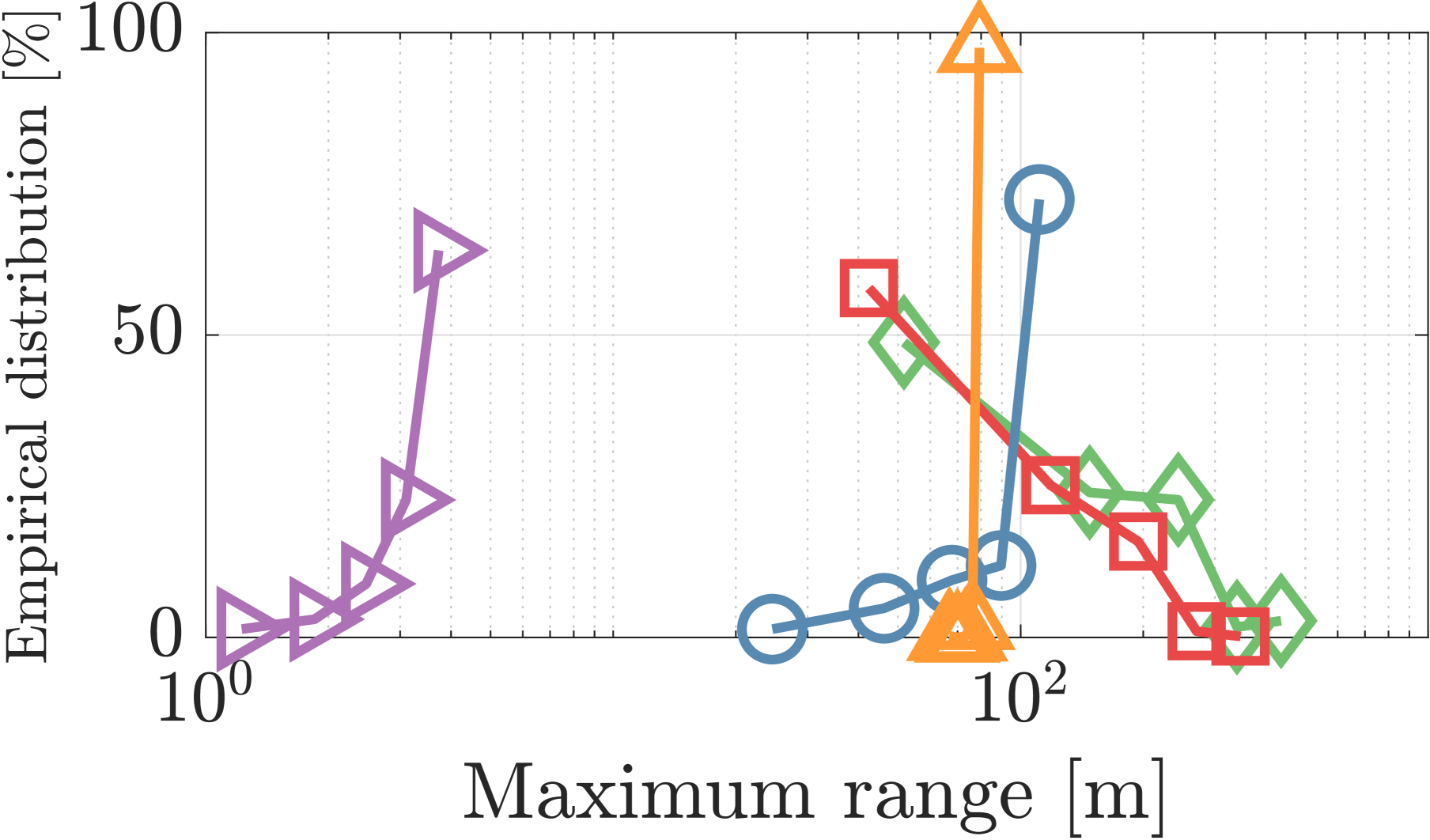
(b)

Fig. 2: (a) Variation in the number of points after voxelization at different voxel sizes $v$ for multiple datasets. Note that even in indoor environments, the number of points varies significantly depending on the sensor (i.e.,TIERS [60] from three different LiDAR sensors vs. 3DMatch [88] from an RGB-D camera). Additionally, even both TIERS and KITTI are acquired using the same sensor type (i.e., omnidirectional LiDAR sensors), the number of voxel-sampled points can differ greatly depending on the environment (i.e.,TIERS, collected in indoor scenes vs. KITTI [28], acquired in outdoor environments using a 64-channel LiDAR sensor). (b) Empirical distribution of the datasets’ maximum range.

3.2 Key observations

If $\mathcal{A}$ in 1 is accurate, solving 1 is easy. However, we have observed there exist three factors that cause learning-based registration to struggle in estimating $\mathcal{A}$ when given out-of-domain data.

3.2.1 Voxel size and search radius

First, dependencies of optimal search radius $r$ for local descriptors and voxel size $v$ for each dataset are problematic. The optimal parameters vary significantly across datasets due to differences in scale and point density (e.g., small indoor scenes vs. large outdoor spaces [5]) Consequently, improper $r$ or $v$ can severely degrade registration performance by failing to account for specific scale and density characteristics of a given environment or sensor; see Sec. 5.1. For instance, in Fig. 2(a), as $v$ controls the maximum number of points that can be fed into the network, a too-small $v$ can trigger out-of-memory errors when outdoor data processed with parameters optimized for indoor environments are taken as input to the network.

In particular, most methods heavily depend on manual tuning, which hinders generalization. Therefore, we employ a geometric bootstrapping to adaptively determine $v$ and $r$ at test time based on the scale and point density of the given input clouds; see Sec. 4.1.

3.2.2 Input scale normalization

Next, directly feeding raw $x$, $y$, and $z$ values into the network leads to strong in-domain dependency [32, 59]. That is, when a model fits to the training distribution, large scale discrepancies between training and unseen data can cause catastrophic failure (see Fig. 2(b) for an example of maximum range discrepancy). For this reason, we conclude that normalizing input points within local neighborhoods (or patches) is necessary to achieve generalizability, ensuring that their coordinates lie within a bounded range (e.g., $[-1,1]$) [6, 5].

Based on these insights, we adopt patch-based descriptor generation as our pipeline for descriptor matching; see Sec. 4.2.

3.2.3 Keypoint detection

Following Sec. 3.2.2, we observed that point-wise feature extractor modules in existing methods [32, 59, 80] are empirically brittle to out-of-domain data. Because failed keypoint detection leads to the selection of unreliable and non-repeatable points as keypoints, it results in low-quality descriptors and ultimately degrades the quality of $\mathcal{A}$ [30].

An interesting observation is that replacing the learning-based detector with the farthest point sampling (FPS) preserves registration performance. For this reason, we adopt FPS over a learning-based module (see Sec. 5.3). Specifically, we apply it separately at local, middle, and global scales to account for multi-scale variations.

4 BUFFER-X

Building upon our key observations in Sec. 3.2, we present our multi-scale zero-shot registration pipeline; see Fig. 3. First, the appropriate voxel size and radii for each cloud pair are predicted by geometric bootstrapping (Sec. 4.1), considering the overall distribution of cloud points and the density of neighboring points, respectively. Then, we extract Mini-SpinNet-based features [5] for the sampled points via FPS at multiple scales (Sec. 4.2). Finally, at the intra- and cross-scale levels, refined correspondences are estimated based on consensus maximization [68, 67, 89] (Sec. 4.3) and serve as input for the final relative pose estimation using a solver.

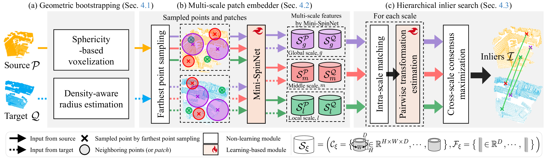
Fig. 3: Overview of our BUFFER-X, which mainly consists of three steps. (a) Geometric bootstrapping (Sec. 4.1) to determine the appropriate voxel size and radii for the given source $\mathcal{P}$ and target $\mathcal{Q}$ clouds. (b) Multi-scale patch embedder (Sec. 4.2) to generate patch-wise descriptor $\mathcal{S}_{\xi}$ for multiple scale $\xi\in\{l,m,g\}$, where $l$, $m$, and $g$ represent local, middle, and global scales, respectively. Specifically, Mini-SpinNet [5] outputs cylindrical feature maps $\mathcal{C}_{\xi}$ and vector feature set $\mathcal{F}_{\xi}$. (c) Hierarchical inlier search (Sec. 4.3), which first performs nearest neighbor-based intra-scale matching using $\mathcal{F}^{\mathcal{P}}_{\xi}$ and $\mathcal{F}^{\mathcal{Q}}_{\xi}$ at each scale, followed by pairwise transformation estimation. Finally, it identifies globally consistent inliers $\mathcal{I}$ across all scales to refine correspondences based on consensus maximization [68, 89].

4.1 Geometric bootstrapping

Sphericity-based voxelization. First, we determine proper voxel size $v$ by leveraging sphericity, quantified using eigenvalues [29, 1], to reflect how the cloud points are dispersed in space. To this end, we apply principal component analysis (PCA) [42] to the covariance of sampled points, which can efficiently capture point dispersion by analyzing eigenvalues while remaining computationally lightweight.

Formally, let $h(\mathcal{P},\mathcal{Q})$ be a function that selects the larger point cloud based on cardinality, let $g(\mathcal{P},\delta)$ be a function that samples $\delta\%$ of points from a given point cloud, and let ${\bm{C}}\in\mathbb{R}^{3\times 3}$ be the covariance of $g(h(\mathcal{P},\mathcal{Q}),\delta_{v})$, where $\delta_{v}$ is a user-defined sampling ratio. Then, using PCA, three eigenvalues $\lambda_{a}$ and their corresponding eigenvectors ${\bm{v}}_{a}$ are calculated as follows:

$${\bm{C}}{\bm{v}}_{a}=\lambda_{a}{\bm{v}}_{a},\quad a\in\{1,2,3\},$$ (2)

which are assumed to be $\lambda_{1}\geq\lambda_{2}\geq\lambda_{3}$. Then, using these properties, we can compute the sphericity $\frac{\lambda_{3}}{\lambda_{1}}$ [1], which quantifies how evenly a point cloud is distributed in space. Since LiDAR points are primarily distributed along the sensor’s horizontal plane (i.e., forming a disc-like shape), $\frac{\lambda_{3}}{\lambda_{1}}$ tends to be low compared to RGB-D point clouds.

In addition, as observed in Fig. 2(a), LiDAR point clouds require a larger voxel size; thus, we set $v$ as follows:

$$v=\begin{cases}\kappa_{\text{spheric}}\sqrt{s},&\text{if}\;\frac{\lambda_{3}}{\lambda_{1}}\geq\tau_{v},\\ \kappa_{\text{disc}}\sqrt{s},&\text{otherwise},\end{cases}$$ (3)

where $\kappa_{\text{spheric}}$ and $\kappa_{\text{disc}}$ are constant user-defined coefficients across all datasets, satisfying $\kappa_{\text{spheric}}<\kappa_{\text{disc}}$, $\tau_{v}$ is a user-defined threshold, and $s$ is the length that represents the spread of points along the eigenvector corresponding to the smallest eigenvalue ${\bm{v}}_{3}$ (i.e., $s=\max(\mathcal{P}_{\text{sampled}}\cdot{\bm{v}}_{3})-\min(\mathcal{P}_{\text{sampled}}\cdot{\bm{v}}_{3})$). Consequently, as $\frac{\lambda_{3}}{\lambda_{1}}$ and $s$ adapt based on the environment (i.e., indoor or outdoor) and the field of view of the sensor type (i.e., RGB-D or LiDAR point cloud), 3 enables the adaptive setting of $v$.

Hereafter, for brevity, we denote $f_{v}(\mathcal{P})$ and $f_{v}(\mathcal{Q})$ simply as $\mathcal{P}$ and $\mathcal{Q}$, respectively,

Density-aware radius estimation. Next, in contrast to some state-of-the-art approaches [5, 6] that use a single fixed user-defined search radius, we determine $r$ at local, middle, and global scales, respectively, by considering the input point densities. Let neighboring search function within the radius $r$ around a query point ${\bm{p}}_{q}$ be:

$$\mathcal{N}\big{(}{\bm{p}}_{q},\mathcal{P},r\big{)}=\big{\{}{\bm{p}}\in\mathcal{P}|\;\|{\bm{p}}-{\bm{p}}_{q}\|_{2}\leq r\big{\}}.$$ (4)

Then, as presented in Fig. 4(a), the radius for patch-wise descriptor generation for each scale $r_{\xi}$ is defined as follows:

$$r_{\xi}=\operatorname*{arg\,min}_{r}\left|\frac{1}{N}\sum_{{\bm{p}}_{q}\in\mathcal{P}_{r}}\text{card}\Big{(}\mathcal{N}\big{(}{\bm{p}}_{q},\mathcal{P}_{r},r\big{)}\Big{)}-\tau_{\xi}\right|,$$ (5)

where $\xi\in\{l,m,g\}$ denotes the scale level (i.e., local, middle, and global scale, respectively), $\tau_{\xi}$ denotes the user-defined threshold, which represents the desired neighborhood density (i.e., average proportion of neighboring points relative to the total number of points), satisfying $\tau_{l}\leq\tau_{m}\leq\tau_{g}$ (accordingly, $r_{l}\leq r_{m}\leq r_{g}$ as presented in Fig. 4(a)), and $\mathcal{P}_{r}$ is a set of $N_{r}$ points sampled from $h(\mathcal{P},\mathcal{Q})$, where $N_{r}$ is a user-defined parameter for radius estimation. To account for cases where the points are too sparse, we set the maximum truncation radius $r_{\text{max}}$ as $r_{\xi}\leftarrow\text{max}(r_{\xi},r_{\text{max}})$.

4.2 Multi-scale patch embedder

Next, with the voxelized point clouds $\mathcal{P}$ and $\mathcal{Q}$ and radii estimated by 5, patch-wise descriptors are generated at each scale.

Farthest point sampling. As discussed in Sec. 3.2.3, we sample ${\mathcal{P}_{\xi}}$ from $\mathcal{P}$ at each scale using FPS to be free from a learning-based keypoint detector (resp. ${\mathcal{Q}_{\xi}}$ from $\mathcal{Q}$). Note that instead of extracting local, middle, and global-scale descriptors for the same sampled point [85], we independently sample separate points for each scale, as illustrated in Fig. 3(b). This is because we empirically found that different regions may require distinct scales for optimal feature extraction; see Sec. 5.3.

Mini-SpinNet-based descriptor generation. Using multiple radii $r_{\xi}$, we sample patches at three distinct scales, providing a more comprehensive multi-scale representation. Then, we use Mini-SpinNet[5] for descriptor generation, which is a lightweight version of SpinNet [6].

In particular, building on the insights from Sec. 3.2.2, we ensure the scale of points in each patch is normalized to a bounded range of $[-1,1]$ by dividing by $r_{\xi}$; see Fig. 4(b). By doing so, we can resolve the dependency on the in-domain scale. To maintain consistency across patches at all scales, we fix the patch size to $N_{\text{patch}}$ and randomly sample when a patch exceeds this size, ensuring a consistent number of points regardless of scale variations.

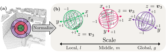
Fig. 4: (a) Visual description of local ($r_{l}$), middle ($r_{m}$), and global ($r_{g}$) radii for the same point to illustrate scale differences and (b) normalized patches ranging from $[-1,1]$. Note that their reference frames follow the eigenvectors obtained from principal component analysis (PCA) [42, 1]. The $z$-axis is assigned to the eigenvector ${\bm{v}}_{3}$, which corresponds to the smallest eigenvalue.

Finally, taking these normalized patches as inputs, Mini-SpinNet outputs a superset $\mathcal{S}^{\mathcal{P}}_{\xi}$ consisting of $D$-dimensional feature vectors $\mathcal{F}^{\mathcal{P}}_{\xi}$ and cylindrical feature maps $\mathcal{C}^{\mathcal{P}}_{\xi}$, where corresponds to ${\mathcal{P}_{\xi}}$ (resp. $\mathcal{S}^{\mathcal{Q}}_{\xi}$ consisting of $\mathcal{F}^{\mathcal{Q}}_{\xi}$ and $\mathcal{C}^{\mathcal{Q}}_{\xi}$ from ${\mathcal{Q}_{\xi}}$), as described in Fig. 3. Note that while BUFFER [5] utilizes learned reference axes to extract cylindrical coordinates, our approach defines the reference axes for each patch by applying PCA to the covariance of points within the patch, setting the $z$-direction as ${\bm{v}}_{3}$ (as in 2 and illustrated by $z={\bm{v}}_{3}$ in Fig. 4(b)), to eliminate potential dataset-specific inductive biases.

4.3 Hierarchical inlier search

Here, we first perform inter-scale matching to get initial correspondences $\mathcal{A}_{\xi}$ at each scale and then establish cross-scale consistent correspondences in a consensus maximization manner.

Intra-scale matching. First, we perform nearest neighbor-based mutual matching [47] between $\mathcal{F}^{\mathcal{P}}_{\xi}$ and $\mathcal{F}^{\mathcal{Q}}_{\xi}$, yielding matched correspondences $\mathcal{A}_{\xi}$ at each scale. Using $\mathcal{A}_{\xi}$, we extract the corresponding elements from $\mathcal{C}^{\mathcal{P}}_{\xi}$ and $\mathcal{C}^{\mathcal{Q}}_{\xi}$, denoted as $\widehat{\mathcal{C}}^{\mathcal{P}}_{\xi}$ and $\widehat{\mathcal{C}}^{\mathcal{Q}}_{\xi}$, and the sampled keypoints from ${\mathcal{P}_{\xi}}$ and ${\mathcal{Q}_{\xi}}$ as $\widehat{\mathcal{P}}_{\xi}$ and $\widehat{\mathcal{Q}}_{\xi}$, respectively (i.e., $|\mathcal{A}_{\xi}|=|\widehat{\mathcal{C}}^{\mathcal{P}}_{\xi}|=|\widehat{\mathcal{C}}^{\mathcal{Q}}_{\xi}|=|\widehat{\mathcal{P}}_{\xi}|=|\widehat{\mathcal{Q}}_{\xi}|$).

Pairwise transformation estimation. Next, using each cylindrical feature pair ${\bm{c}}^{{\bm{p}}}\in\widehat{\mathcal{C}}^{\mathcal{P}}_{\xi}$ and ${\bm{c}}^{{\bm{q}}}\in\widehat{\mathcal{C}}^{\mathcal{Q}}_{\xi}$ at each scale, each of whose size is $\mathbb{R}^{H\times W\times D}$, we calculate pairwise 3D relative transformation between two patches. Here, $H$, $W$, and $D$ denote the height, sector size for the yaw direction along the $z$-axis of the reference axes, and feature dimensionality of a cylindrical feature, respectively.

As mentioned earlier, since the cylindrical feature is aligned with the local reference axes via PCA, the relative 3D rotation between ${\bm{v}}^{\bm{p}}_{3}$ (resp. ${\bm{v}}^{\bm{q}}_{3}$) and the unit $z$-axis, ${\bm{z}}=[0\;0\;1]^{\intercal}$, can be calculated using Rodrigues’ rotation formula [48] as follows:

$${\bm{R}}^{{\bm{p}}}={\bm{I}}+\sin(\theta^{{\bm{p}}})[{\bm{n}}^{{\bm{p}}}]_{\times}+\big{(}1-\cos(\theta^{{\bm{p}}})\big{)}[{\bm{n}}^{{\bm{p}}}]_{\times}^{2},$$ (6)

where ${\bm{n}}^{{\bm{p}}}={\bm{v}}^{{\bm{p}}}_{3}\times{\bm{z}}$, $\theta^{{\bm{p}}}=\cos^{-1}\left({\bm{v}}^{{\bm{p}}}_{3}\cdot{\bm{z}}\right)$, and $[\cdot]_{\times}$ denotes the skew operator (resp. ${\bm{R}}^{\bm{q}}$). Thus, once the yaw rotation between the two patches ${\bm{R}}_{\text{yaw}}$ is determined, the full 3D rotation can be obtained as ${\bm{R}}=\left({\bm{R}}^{\bm{q}}\right)^{\intercal}{\bm{R}}_{\text{yaw}}{\bm{R}}^{\bm{p}}$.

As explained by Ao  et al. [5], ${\bm{c}}^{{\bm{p}}}$ and ${\bm{c}}^{{\bm{q}}}$ follow discretized SO(2)-equivariant representation; thus, by finding the yaw rotation that maximizes circular cross-correlation between ${\bm{c}}^{{\bm{p}}}$ and ${\bm{c}}^{{\bm{q}}}$, we can estimate the relative SO(2) rotation ${\bm{R}}_{\text{yaw}}$. To this end, a 4D matching cost volume ${\bm{V}}\in\mathbb{R}^{H\times W\times W\times D}$ is constructed to represent the sector-wise differences between ${\bm{c}}^{{\bm{p}}}$ and ${\bm{c}}^{{\bm{q}}}$. Then, ${\bm{V}}$ is processed by a 3D cylindrical convolutional network (3DCCN) [6], mapping ${\bm{V}}$ to a score vector ${\bm{\beta}}$ of size $W$.

By applying the softmax operation $\sigma(\cdot)$ to ${\bm{\beta}}$, we obtain $\sigma({\bm{\beta}})$, where the $w$-th element $\sigma_{w}({\bm{\beta}})\in[0,1]$ represents the probability mass assigned to the discrete yaw rotation index $w$. Using this distribution, the discrete rotation offset $d$ is computed as follows:

$$d=\sum_{w=1}^{W}\sigma_{w}({\bm{\beta}})\times w.$$ (7)

Finally, ${\bm{R}}_{\text{yaw}}$ is calculated as follows:

$${\bm{R}}_{\text{yaw}}=\begin{bmatrix}\cos\left(\frac{2\pi d}{W}\right)&-\sin\left(\frac{2\pi d}{W}\right)&0\\ \sin\left(\frac{2\pi d}{W}\right)&\cos\left(\frac{2\pi d}{W}\right)&0\\ 0&0&1\end{bmatrix}.$$ (8)

Subsequently, the translation vector is given by ${\bm{t}}={\bm{q}}-{\bm{R}}{\bm{p}}$, where ${\bm{p}}\in\widehat{\mathcal{P}}_{\xi}$ and ${\bm{q}}\in\widehat{\mathcal{Q}}_{\xi}$ are a matched point pair.

Cross-scale consensus maximization. Then, using per-pair $({\bm{R}},{\bm{t}})$ estimates from all scales, the 3D point pairs with the largest cardinality across scales should be selected as the final inlier correspondences $\mathcal{I}$, ensuring cross-scale consistency. To achieve this, we formulate the cross-scale inlier selection as consensus maximization problem [68, 89].

Formally, by denoting $N=\sum_{\xi}|\mathcal{A}_{\xi}|$, let $({\bm{R}},{\bm{t}})\in\mathcal{T}$ be a candidate transformation set of size $N$, and let $({\bm{p}}_{n},{\bm{q}}_{n})\in\mathcal{D}$ be the set of matched point pairs, where $n\in\{1,\dots,N\}$, ${\bm{p}}_{n}\in\bigcup_{\xi}\widehat{\mathcal{P}}_{\xi}$ and ${\bm{q}}_{n}\in\bigcup_{\xi}\widehat{\mathcal{Q}}_{\xi}$. Then, $\mathcal{I}$ is estimated as follows:

$$\max_{({\bm{R}},{\bm{t}})\in\mathcal{T},\;\mathcal{I}}|\mathcal{I}|$$ (9)

$$\text{s.t.}~~\|{\bm{R}}{\bm{p}}_{n}+{\bm{t}}-{\bm{q}}_{n}\|_{2}<\epsilon,~~\forall({\bm{p}}_{n},{\bm{q}}_{n})\in\mathcal{I}\subseteq\mathcal{D},$$

where $\epsilon$ is an inlier threshold.

Finally, $\mathcal{I}$ is given as input to a solver, such as RANSAC [27] or TEASER++ [77] to estimate $\hat{{\bm{R}}}$ and $\hat{{\bm{t}}}$. For a fair comparison with existing approaches, we use RANSAC.

4.4 Loss function and training

Loss functions. Unlike BUFFER, which was trained in four stages, our network follows a relatively simpler two-stage training process thanks to its detector-free nature. First, we train the feature discriminability of Mini-SpinNet descriptors using contrastive learning [82], followed by training $d$ in 7 to improve transformation estimation accuracy.

In particular, we employ the Huber loss [92] $\rho_{\text{Huber}}(\cdot)$ for training $d$ to remain robust to outliers[9], while balancing sensitivity to small errors, which is formulated as follows:

$$\rho_{\text{Huber}}(r)=\begin{cases}\frac{1}{2}r^{2},&\text{if }|r|\leq\delta\\ \delta(|r|-\frac{1}{2}\delta),&\text{otherwise},\end{cases}$$ (10)

where $r$ denotes the residual and $\delta$ denotes the user-defined truncation threshold. Then, denoting the total number of data pairs by ${N_{d}}$, the $\gamma$-th predicted offset by $d_{\gamma}$, and the corresponding ground-truth offset by $d^{*}_{\gamma}$, the loss function $\mathcal{L}_{d}$ is defined as follows:

$$\mathcal{L}_{d}=\frac{1}{N_{d}}\sum_{\gamma=1}^{N_{d}}\rho_{\text{Huber}}(d_{\gamma}-d^{*}_{\gamma}).$$ (11)

Patch distribution augmentation. Furthermore, we propose an inter-patch point distribution augmentation to allow Mini-SpinNet to experience a wider variety of patch distribution patterns. Specifically, we empirically sample the radius within $[\frac{2}{3}r,\frac{4}{3}r]$ based on a uniform probability. As mentioned in Sec. 4.2, since $N_{\text{patch}}$ points within the radius are randomly selected as an input, a diverse set of patterns can be provided as $r$ varies.

Notably, training is conducted using only a single scale. This leverages the scale normalization characteristic of BUFFER-X, making it unnecessary to train with multi-scale separately.

5 Experiments

Datasets. As presented in Table 1, we designed our generalizability benchmark using eleven different datasets [88, 32, 81, 60, 69, 28, 56, 34, 71, 61] to ensure balanced consideration of the following aspects: a) variation in environmental scales (i.e., indoor and outdoor environments), b) different scanning patterns with different sensor types; see “Sensor Type” column in Table 1, c) acquisition setups, and d) diversity of geographic and cultural environments as the data was collected across Europe, Asia, and the USA (i.e., Oxford, KAIST, and MIT campuses, respectively). More details can be found in Appendices B and C.

	Dataset Name	Env.	Sensor Type	Acquisition	Range [m]	# Pairs
Indoor	3DMatch [88]	Room	RGB-D cameras	Handheld	3.5	1,623
	3DLoMatch [32]	Room	RGB-D cameras	Handheld	3.5	1,781
	ScanNet++i [81]	Room	iPhone 13 Pro${}^{\text{\char 93}}$	Handheld	3.5	2,074
	ScanNet++F [81]	Room	FARO (Stationary LiDAR)	Tripod	7.0	2,016
	TIERS [60]	Room, Interior	VLP16, OS1-64, OS0-128	Cart	110	870
Outdoor	WOD [69]	City	Laser Bear Honeycomb${}^{\text{\char 93}}$	Vehicle	75	130
	KITTI [28]	City	HDL-64E	Vehicle	80	555
	ETH [56]	Forest	Rotating 2D Scanner	Tripod	30	713
	KAIST (from HeLiPR [34])	Campus	OS2-128, Livox Avia${}^{\text{\char 93}}$, Aeva Aeries II${}^{\text{\char 93}}$	Vehicle	240	1,991
	MIT (from Kimera-Multi [14])	Campus	VLP16	Wheeled	100	230
	Oxford (from NewerCollege [61])	Campus	OS1-64	Quadruped / Handheld	100	301

Table 1: Overview of datasets used in our experiments, categorized by the environment, measurement sensor type, acquisition setup, average maximum range, and a number of test pairs. The superscript ✽ highlights solid-state LiDAR sensors to especially emphasize that our evaluation is not limited to conventional omnidirectional spinning LiDAR sensors, but contains different scanning patterns.

Training settings. Then, we only train the network on a single dataset, such as 3DMatch [88] or KITTI [28]. Using the same hyperparameters of BUFFER [5], we conducted a two-stage optimization (i.e., Mini-SpinNet is first trained, followed by training the 3DCCN) and we used Adam optimizer [35] with a learning rate of 0.001, a weight decay of 1e-6, and a learning rate decay of 0.5. We used NVIDIA GeForce RTX 3090 with AMD EPYC 7763 64-Core.

Testing settings. In the case of the existing datasets [88, 32, 69, 28, 56], we follow the conventional given pairs. The description of the newly employed datasets for evaluation can be found in Appendix B.

Evaluation Metrics. As a key metric, we use the success rate, which directly assesses the robustness of global registration [40]. Specifically, a registration is deemed successful if the translation and rotation errors are within $\tau_{\text{trans}}$ and $\tau_{\text{rot}}$, respectively [82]. For successful cases, we evaluated the performance using relative translation error (RTE) and relative rotation error (RRE), which are defined as follows:

• $\text{RTE}=\sum_{n=1}^{N_{\text{success}}}({\bm{t}}_{n,\text{GT}}-{\hat{{\bm{t}}}}_{n})^{2}/N_{\text{success}}$,

• $\text{RRE}=\frac{180}{\pi}\sum_{n=1}^{N_{\text{success}}}|\cos^{-1}(\frac{\operatorname{Tr}\left({\hat{{\bm{R}}}}_{n}^{\intercal}{\bm{R}}_{n,\text{GT}}\right)-1}{2})|/N_{\text{success}}$

where ${\bm{t}}_{n,\text{GT}}$ and ${\bm{R}}_{n,\text{GT}}$ denote the $n$-th ground truth translation and rotation, respectively; $N_{\text{success}}$ represents the number of successful registration. The more detailed criteria for determining a successful registration are provided in table A2.

	Env.	Indoor					Outdoor						Average rank
	Dataset	3DMatch	3DLoMatch	ScanNet++i	ScanNet++F	TIERS	KITTI	WOD	KAIST	MIT	ETH	Oxford
Conven- tional	FPFH [63] + FGR [94] +	62.53	15.42	77.68	92.31	80.60	98.74	100.00	89.80	74.78	91.87	99.00	9.55
	FPFH [63] + Quatro [43] +	8.22	1.74	9.88	97.27	86.57	99.10	100.00	91.46	79.57	51.05	91.03	10.73
	FPFH [63] + TEASER++ [77] +	52.00	13.25	66.15	97.22	73.13	98.92	100.00	89.20	71.30	93.69	99.34	10.00
Deep learning-based	FCGF [22]	88.18	40.09	72.90	88.69	55.96	0.00	0.00	0.00	0.00	54.98	0.00	15.00
	+	88.18	40.09	85.87	88.69	78.62	90.27	97.69	92.91	92.61	54.98	93.68	10.18
	+ +	88.18	40.09	85.87	88.69	80.11	94.41	97.69	93.55	93.04	55.53	95.68	9.55
	Predator [32]	90.60	62.40	75.94	N/A	N/A	N/A	N/A	N/A	N/A	N/A	N/A	15.73
	+	90.60	62.40	75.94	29.81	56.44	0.00	0.00	0.95	0.00	0.14	0.33	14.55
	+ +	90.60	62.40	75.94	86.01	75.74	77.29	86.92	87.09	79.56	54.42	93.68	11.82
	GeoTransformer [59]	92.00	75.00	91.18	N/A	N/A	N/A	N/A	N/A	N/A	N/A	N/A	14.00
	+	92.00	75.00	91.18	7.54	5.06	0.36	0.77	0.25	0.87	0.00	0.33	13.09
	+ +	92.00	75.00	92.72	97.02	92.99	92.43	89.23	91.86	95.65	71.53	97.01	6.27
	BUFFER [5]	92.90	71.80	92.72	93.75	62.30	0.00	1.54	0.50	6.96	97.62	0.66	10.45
	+	92.90	71.80	93.01	94.69	88.96	99.46	100.00	97.24	95.65	99.30	99.00	3.82
	+ +	92.90	71.80	93.01	94.69	88.96	99.46	100.00	97.24	95.65	99.30	99.00	3.82
	PARENet [80]	95.00	80.50	90.84	N/A	N/A	N/A	N/A	N/A	N/A	N/A	N/A	13.27
	+	95.00	80.50	90.84	43.75	6.21	0.18	0.77	0.75	1.30	1.40	1.66	11.55
	+ +	95.00	80.50	90.84	87.95	75.06	84.86	92.31	86.44	84.78	69.42	93.36	8.82
	Ours with only $r_{m}$	93.38	71.69	93.10	99.60	90.80	99.82	100.00	99.05	95.65	99.30	99.34	3.00
	Ours	95.58	74.18	94.99	99.90	93.45	99.82	100.00	99.15	97.30	99.72	99.67	1.55

Table 2: Quantitative performance comparison on rate to evaluate generalization capability. Deep learning-based models were trained only on 3DMatch [88] and RANSAC was used with the maximum iteration of 50K. The icons represent oracle tuning () to set proper voxel size and search radius to each dataset, and scale alignment () to normalize dataset scales to be similar to that of 3DMatch data (e.g., the scale of KITTI, which typically uses a voxel size of 0.3 m, is adjusted to match the scale of 3DMatch, which typically uses a voxel size of 0.025 m, by dividing by $\frac{0.3}{0.025}$).

5.1 Analyses on the generalization

First, we demonstrate that existing methods struggle in achieving out-of-the-box generalization, leading to performance degradation due to the issues explained in Sec. 3. In this experiment, we mainly used renowned learning-based approaches: FCGF [22], Predator [32], GeoTransformer (GeoT for brevity) [59], BUFFER [5], and PARENet [80].

As shown in Table 2, models trained with small voxel sizes and search radii for indoor datasets exhibited substantial performance degradation in outdoor scenarios. In particular, as explained in Sec. 3.2.1, we observed that some approaches even did not work due to out-of-memory issues (i.e., N/A in Table 2) caused by an excessively large number of input points.

Once a properly user-tuned voxel size and search radius were provided (referred to as oracle tuning, ), BUFFER showed a remarkable performance increase owing to its patch-wise input scale normalization characteristics. In contrast, other approaches still showed relatively lower success rates because the networks received point clouds with magnitudes not encountered during training. This potential limitation is further evidenced by the performance improvement of Predator after scale alignment, supporting our claim that scale normalization is a key factor in achieving generalizability.

5.2 Performance comparison

Second, we demonstrate that our proposed algorithm, inspired by these key observations, achieves substantial out-of-the-box generalization; see Table 2. In particular, our approach achieved lower RTE and RRE than state-of-the-art approaches even with oracle tuning and scale alignment (Fig. 5), while maintaining competitive in-domain performance (Table 3). Therefore, this experimental evidence supports our claim that our algorithm achieves a high generalization capability and successfully performs in-domain scenarios.

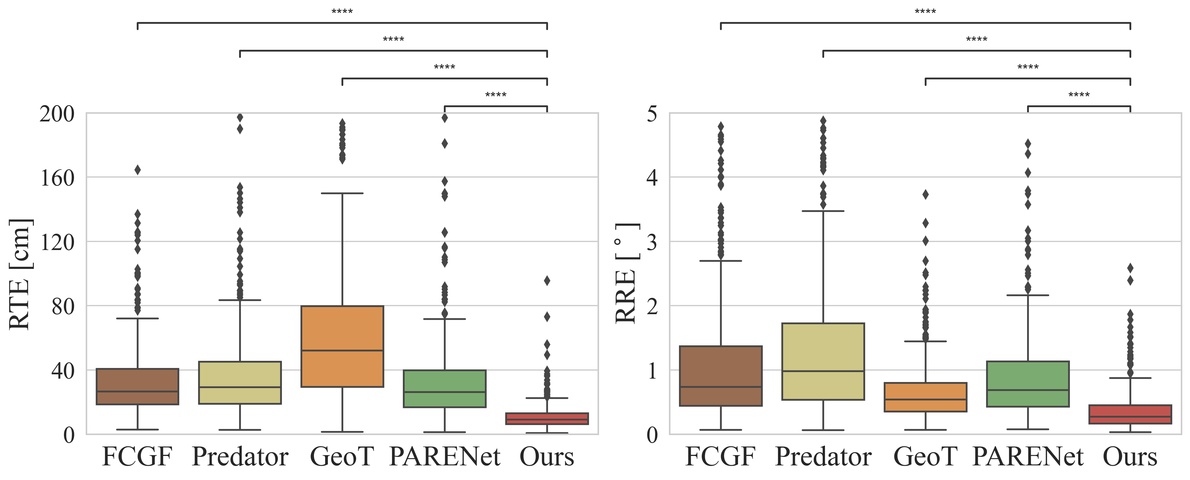
Fig. 5: Relative translation error (RTE) and relative rotation error (RRE) of our approach to state-of-the-art methods, all trained on 3DMatch and tested on KITTI, with oracle tuning and scale alignment, corresponding to those in Table 2 under the + + setting. The **** annotations indicate measurements with a $p$-value $<10^{-4}$ after a paired $t$-test.

	Method	RTE [cm] $\downarrow$	RRE [°] $\downarrow$	Succ. rate [%] $\uparrow$
Conventional.	G-ICP [66]	8.56	0.22	37.95
	FPFH [63] + FGR [94]	18.75	0.38	98.74
	FPFH [63] + Quatro [43]	18.56	0.93	99.10
	FPFH [63] + TEASER++ [77]	15.35	0.68	98.92
	KISS-Matcher [41]	21.33	0.96	99.46
Learning-based	3DFeat-Net [82]	25.90	0.57	95.97
	FCGF [22]	6.47	0.23	98.92
	DIP [53]	8.69	0.44	97.30
	Predator [32]	5.60	0.24	99.82
	SpinNet [6]	9.88	0.47	99.10
	CoFiNet [85]	8.20	0.41	99.82
	D3Feat [8]	11.00	0.24	99.82
	GeDi [54]	7.55	0.33	99.82
	GeoTransformer [59]	7.40	0.27	99.82
	BUFFER [5]	7.46	0.26	99.64
	PARE-Net [80]	4.90	0.23	99.82
	Proposed	7.74	0.27	99.82

Table 3: In-domain quantitative results in terms of relative translation error (RTE), relative rotation error (RRE), and success rate on KITTI [82].

5.3 Ablation study

Impact of geometric bootstrapping. Fig. 6 supports our claim that voxel size and radius have a more direct impact on performance than expected. Unlike BUFFER, which relies on manual tuning, our method automatically estimates optimal $v$ and $r$, adapting to different scenes and maintaining consistency across varying dataset densities (Fig. 6(b)).

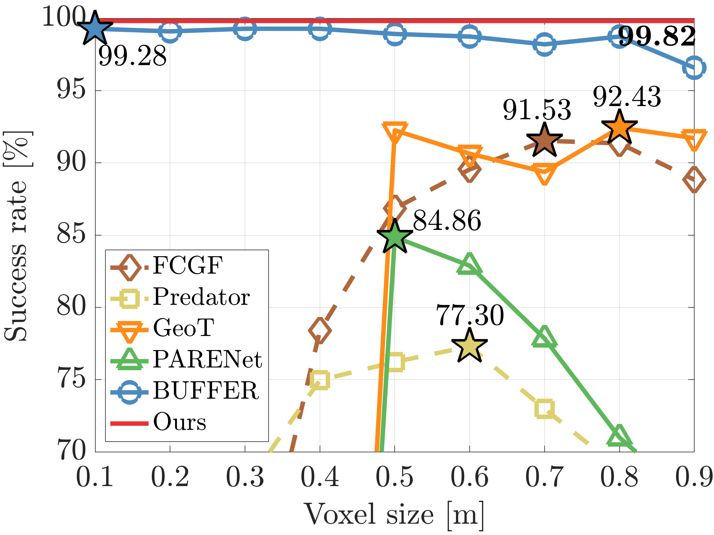
(a)

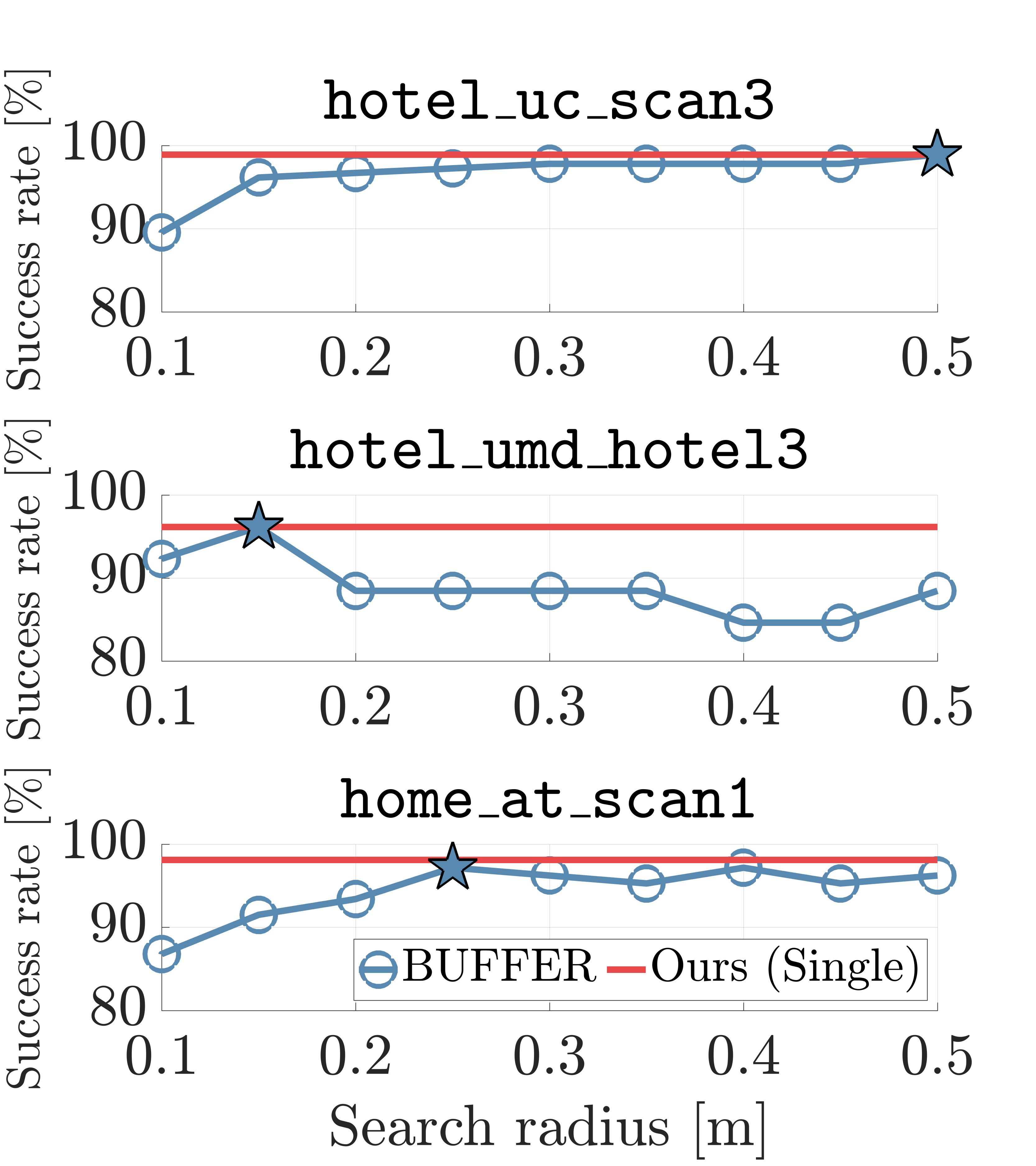
(b)

Fig. 6: Success rate changes of state-of-the-art approaches based on the voxel size and search radius, where ★ indicates the best performance after tuning. (a) Impact of voxel size on success rate for models trained on 3DMatch with scale alignment, evaluated on KITTI. (b) Comparison of our BUFFER-X and BUFFER with varying search radius, highlighting that the optimal radius might differ even within the same dataset. For a fair comparison, BUFFER-X is evaluated in single-scale mode.

Learning-based detector vs. Farthest point sampling. Interestingly, FPS rather showed better performance than the learning-based keypoint detector in BUFFER[5], even in its training domain (i.e., in 3DMatch and 3DLoMatch). In particular, the performance gap sometimes becomes more pronounced in the out-of-domain scenes, demonstrating that robust cross-domain generalization can be achieved without the need for additional learning-based keypoint selection.

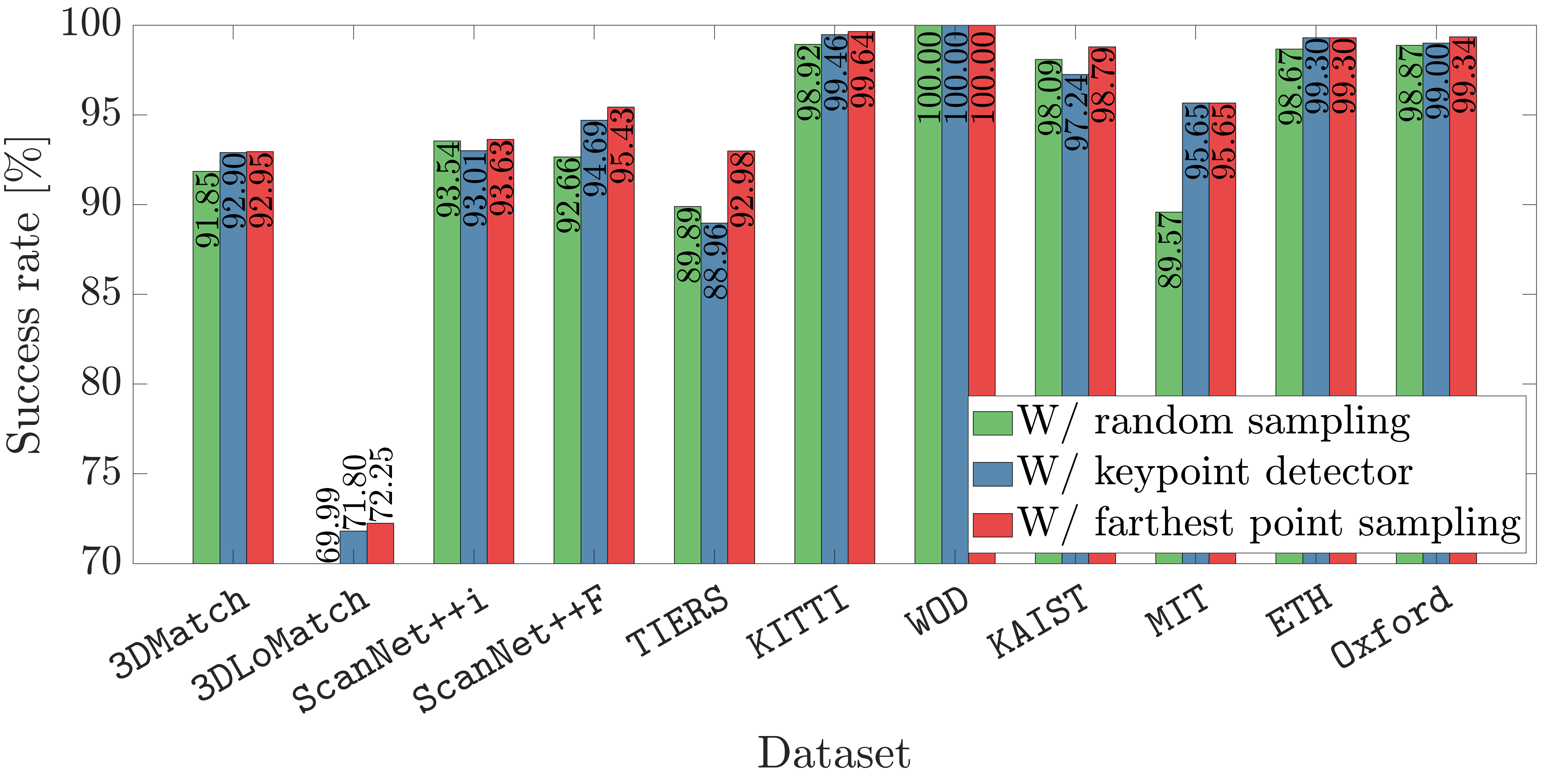
Fig. 7: Comparison of success rates between random sampling, learning-based keypoint detection in BUFFER [5], and our farthest point sampling (FPS) strategy, showing that FPS performs comparably or even better across various datasets.

Impact of multi-scale. While we demonstrated that using only the middle scale in a single-scale setting is comparable to the multi-scale approach (see Table 2), Table 4 shows that incorporating multiple scales further increases the success rate. This implies that correspondences across scales complement each other, leading to higher success rates. However, increasing the number of scales introduces a trade-off between accuracy and computational cost (Fig. 8), allowing users to balance efficiency and performance based on their specific needs.

5.4 Limitations

As seen in Table 2, our approach showed lower success rate in 3DLoMatch, which only have 10-30% overlaps. This is because Eq. 9 selects correspondences with the largest cardinality as inliers. However, in partial overlap scenarios, maximizing the number of correspondences might not yield the actual global optimum (i.e., there might exist $\mathcal{I}^{*}$ that satisfies $|\mathcal{I}^{*}|\leq|\mathcal{I}|$ but leads to a better relative pose estimate). This highlights a trade-off between generalization and robustness to partial overlaps (see Appendix D for further analyses).

Local	Middle	Global	RTE [cm] $\downarrow$	RRE [°] $\downarrow$	Succ. rate [%] $\uparrow$	Hz $\uparrow$
✓			6.57	2.15	84.06	5.61
	✓		5.87	1.85	93.38	5.47
		✓	6.06	1.91	93.57	5.49
✓	✓		5.73	1.81	94.31	2.35
✓		✓	5.77	1.81	94.02	2.36
	✓	✓	5.78	1.81	94.62	2.33
✓	✓	✓	5.78	1.79	95.58	1.81

Table 4: Ablation study: the impact of different scale combinations on registration performance in the 3DMatch [88].

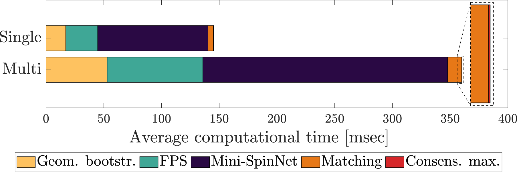
Fig. 8: Area plot of computation time per scale for each module on an NVIDIA GeForce RTX 3090 using 3DMatch [88]. Note that our cross-scale consensus maximization (red) only took 0.40 msec on average.

6 Conclusion

In this study, we addressed the generalization limitations of deep learning-based registration and analyzed key factors hindering it. Based on these insights, we proposed a fully zero-shot pipeline, BUFFER-X, and introduced a comprehensive benchmark for evaluating generalization on real-world point cloud data. In future works, we plan to study how to boost the inference speed for better usability.

A Parameters setup and pseudo code

Here, we summarize the parameter values in Table A1. While some values were set empirically based on prior work, others were tuned to maintain generalizability without dataset-specific fine-tuning. In addition, we also provide pseudo code in Algorithm 1 to outline the core steps of our approach, making it easier to understand the implementation details and facilitate reproducibility.

1 Input:  Source cloud $\mathcal{P}$ and target cloud $\mathcal{Q}$; User-defined parameters $\tau_{v}$, $\delta_{v}$, $\delta_{r}$, $[\tau_{l},\tau_{m},\tau_{g}]$, and $N_{\text{FPS}}$

2 Output: 3D inliers $\mathcal{I}$

3 $\mathcal{P}_{r}\leftarrow\texttt{select\_larger\_cloud}(\mathcal{P},\mathcal{Q})$

4 $\mathcal{P}_{\text{sampled}}=\texttt{sample}(\mathcal{P}_{r},\delta_{v})$ % Sample $\delta_{v}$% of cloud points

5 % Step 1. Geometric bootstrapping

6 $v=\texttt{calc\_voxel\_size}(\mathcal{P}_{\text{sampled}},\tau_{v})$ % See Eq. 3

7 $\mathcal{P}\leftarrow f_{v}(\mathcal{P}),\mathcal{Q}\leftarrow f_{v}(\mathcal{Q})$ % Downsample the point clouds

8 $\mathcal{P}_{r}\leftarrow\texttt{select\_larger\_cloud}(\mathcal{P},\mathcal{Q})$

9 $\mathcal{R}=\texttt{estimate\_radii}(\texttt{sample}(\mathcal{P}_{r},N_{r}),[\tau_{l},\tau_{m},\tau_{g}]),$

10   where $\mathcal{R}=[r_{l},r_{m},r_{g}]$ % See Eq. 5

11 % Step 2. Multi-scale patch embedder

12 $\mathcal{M}^{\mathcal{P}}=\varnothing,\mathcal{M}^{\mathcal{Q}}=\varnothing$ % Containers of embedding output

13 for $r_{\xi}$ in $\mathcal{R}$ do

14    $\mathcal{P}_{\xi}=\texttt{farthest\_point\_sampling}(\mathcal{P},N_{\text{FPS}})$

15    $\mathcal{Q}_{\xi}=\texttt{farthest\_point\_sampling}(\mathcal{Q},N_{\text{FPS}})$

16    $\mathcal{F}^{\mathcal{P}}_{\xi},\mathcal{C}^{\mathcal{P}}_{\xi}=\texttt{MiniSpinNet}(\mathcal{P}_{\xi},\mathcal{P},r_{\xi})$

17    $\mathcal{F}^{\mathcal{Q}}_{\xi},\mathcal{C}^{\mathcal{Q}}_{\xi}=\texttt{MiniSpinNet}(\mathcal{Q}_{\xi},\mathcal{Q},r_{\xi})$

18    $\mathcal{M}^{\mathcal{P}}.\texttt{append}((\mathcal{P}_{\xi},\mathcal{F}^{\mathcal{P}}_{\xi},\mathcal{C}^{\mathcal{P}}_{\xi}))$

19    $\mathcal{M}^{\mathcal{Q}}.\texttt{append}((\mathcal{Q}_{\xi},\mathcal{F}^{\mathcal{Q}}_{\xi},\mathcal{C}^{\mathcal{Q}}_{\xi}))$

20   

21 end for

22% Step 3. Hierarchical inlier search

23 $\mathcal{D}=\varnothing,\mathcal{T}=\varnothing$

24 for $i$ in range(size($\mathcal{M}^{\mathcal{P}}$)) do

25    $(\mathcal{P}_{\xi},\mathcal{F}^{\mathcal{P}}_{\xi},\mathcal{C}^{\mathcal{P}}_{\xi})=\mathcal{M}^{\mathcal{P}}[i]$

26    $(\mathcal{Q}_{\xi},\mathcal{F}^{\mathcal{Q}}_{\xi},\mathcal{C}^{\mathcal{Q}}_{\xi})=\mathcal{M}^{\mathcal{Q}}[i]$

27    % Step 3-1. Nearest neighbor-based intra-scale matching

28    $\mathcal{A}_{\xi}=\texttt{mutual\_matching}(\mathcal{F}^{\mathcal{P}}_{\xi},\mathcal{F}^{\mathcal{Q}}_{\xi})$

29    $(\widehat{\mathcal{P}}_{\xi},\widehat{\mathcal{Q}}_{\xi},\widehat{\mathcal{C}}^{\mathcal{P}}_{\xi},\widehat{\mathcal{C}}^{\mathcal{Q}}_{\xi})=\texttt{filter}(\mathcal{M}^{\mathcal{P}}[i],\mathcal{M}^{\mathcal{Q}}[i],\mathcal{A}_{\xi})$

30    % Step 3-2. Pairwise transformation estimation

31    $\mathcal{T}_{\xi}=\texttt{calc\_pairwise\_R\_and\_t}(\widehat{\mathcal{C}}^{\mathcal{P}}_{\xi},\widehat{\mathcal{C}}^{\mathcal{Q}}_{\xi})$

32    $\mathcal{D}.\texttt{append}(\widehat{\mathcal{P}}_{\xi},\widehat{\mathcal{Q}}_{\xi}))$, $\mathcal{T}.\texttt{append}(\mathcal{T}_{\xi})$

33   

34 end for

35% Step 3-3. Cross-scale consensus maximization

36 $\mathcal{I}=\texttt{consensus\_maximization}(\mathcal{D},\mathcal{T})$ % See Eq. 9

Algorithm 1 BUFFER-X pipeline

B Detailed experimental setups and datasets

Here, we elaborate on the experimental setups that are briefly outlined in Table A2. For widely used datasets, we followed the existing training and testing protocols. The details of the datasets employed in our generalizability benchmark are described as follows.

Param.	Description	Value
$\kappa_{\text{spheric}}$	Coefficient for voxel size when sphericity is high	0.10
$\kappa_{\text{disc}}$	Coefficient for voxel size when sphericity is low	0.15
$\tau_{v}$	Threshold in Eq. 3	0.05
$\tau_{l}$	Threshold for the local ($l$) search radius	0.005
$\tau_{m}$	Threshold for the middle ($m$) search radius	0.02
$\tau_{g}$	Threshold for the local ($g$) search radius	0.05
$\delta_{v}$	Sampling ratio for sphericity-based voxelization	10%
$N_{r}$	Number of sampling points for radius estimation	2,000
$r_{\text{max}}$	Maximum radius	5.0 m
$N_{\text{FPS}}$	Number of sampled points by FPS	1,500
$N_{\text{patch}}$	Maximum number of points in each patch	512
$\delta$	Truncation threshold for Huber loss	1.0
$H$	Height of the cylindrical map in Mini-SpinNet	7
$W$	Sector size of the cylindrical map in Mini-SpinNet	20
$D$	Feature dimension of the cylindrical map in Mini-SpinNet	32

Table A1: Parameters of each module in our BUFFER-X. Note that with this parameter setup, our approach operates in our generalizability benchmark in an out-of-the-box manner without any human intervention.

• 3DMatch follows conventional protocol proposed by Zeng et al.[88].

• 3DLoMatch follows conventional protocol proposed by Huang et al.[32]. This dataset is derived from 3DMatch by selectively extracting pairs with low overlap (i.e., 10–30%), allowing for the evaluation of robustness to low-overlap scenarios.

• ScanNet++F is from ScanNet++ [81]. For each sequence, a pre-merged PLY file representing the entire space is provided, along with the poses of the stationary FARO LiDAR sensor used to measure it. That is, the dataset does not provide individual scans. For that reason, using the given scanner poses, we generate per-scanner point clouds by sampling along raycasting paths from each position within the full map, simulating virtual scans. The sampling process respects the scanner’s horizontal angular resolution as well as its vertical resolution between consecutive rays [64], ensuring a realistic approximation of the original scans. For each ray, the nearest intersecting point in the merged point cloud is selected to simulate the original scan.

• ScanNet++i is also from ScanNet++ [81]. There are depth images captured using a LiDAR sensor attached to an iPhone 13 Pro. These depth images were converted into point clouds using the toolbox provided by 3DMatch [88]. To generate dense point cloud fragments, 50 consecutive frames were accumulated. Finally, pairs with an overlap ratio of at least 0.4 (i.e., 40% overlap between two fragments) were selected as the final test pairs.

• TIERS consists of Indoor06, Indoor08, Indoor09, Indoor10, and Indoor11 sequences in the TIERS dataset [60]. To reduce redundant test pairs, we exclude Indoor07 because it was acquired in the same room as Indoor06.

  In particular, we used data obtained from the Velodyne VLP-16, Ouster OS1-64, and Ouster OS0-128. While more sensors are available, we observed that point clouds from the Livox Horizon and Livox Avia contain too few points. Specifically, when a human surveyor moves close to a wall in an indoor environment, the narrow field of view of these feed-forwarding LiDAR sensors causes only partial wall surfaces to be captured, unlike omnidirectional LiDAR sensors. Additionally, during rotation, there exist segments where the overlap between consecutive scans becomes completely zero, making them unsuitable for the registration problem.

  Dataset/Sequence Name	3DMatch, 3DLoMatch	ScanNet++F	ScanNet++i	TIERS
  Environment	Room	Room, Interior	Room, Interior	Room, Campus Interior
  Acquisition Site	N/A	N/A	N/A	Univ. Turku, Turku, Finland
  Measurement Type	Structured Light	Laser	Laser	Laser
  Employed Sensor(s)	Microsoft Kinect, Structure Sensor, Asus Xtion Pro Live, and Intel RealSense	Faro Focus Premium	Iphone RGB-D Sensor	Velodyne VLP-16, Ouster OS1-64, Ouster0-128
  Approx. Range [m]	3.5	7.0	3.5	110
  # of Points/Frame	336,274	1,381,013	444,876	34,777
  # of Test Pairs	1,623 / 1,781	2,016	2,074	870
  Success Criteria	Follow Zeng et al. [88]’s criteria (Point-wise RMSE $2$ m)	RTE $0.3$ m, RRE $15^{\circ}$	RTE $0.3$ m, RRE $15^{\circ}$	RTE $2.0$ m, RRE $5^{\circ}$

  Dataset/Sequence Name	WOD	KITTI	ETH	KAIST	MIT	Oxford
  Environment	Urban	Urban	Forest	Campus	Campus	Campus
  Acquisition Site	Phoenix, USA	Karlsruhe, Germany	N/A	KAIST campus, Daejeon, South Korea	MIT campus, Cambridge, USA	Oxford campus, London, UK
  Measurement Type	Laser	Laser	Laser	Laser	Laser	Laser
  Employed Sensor(s)	Laser Bear Honeycomb	Velodyne HDL-64E	Rotating Hokuyo UTM-30LX	Livox Avia, Aeva Aeries II, Ouster2-128	Velodyne VLP-16	Ouster OS-1 64
  Approx. Scale [m]	120	80	85	240	100	100
  # Points/Frame	143,960	123,518	96,884	68,790	24,792	55,914
  # of Test Pairs	130	555	713	1,991	230	301
  Success Criteria	RTE $2.0$ m, RRE $5^{\circ}$	RTE $2.0$ m, RRE $5^{\circ}$	RTE $0.3$ m, RRE $2^{\circ}$	RTE $2.0$ m, RRE $5^{\circ}$	RTE $2.0$ m, RRE $5^{\circ}$	RTE $2.0$ m, RRE $5^{\circ}$

  Table A2: Overview of the datasets used in our experiments, including their environments, acquisition sites, measurement types, employed sensors, approximate ranges or scales, and the number of test pairs. The datasets cover a variety of indoor and outdoor environments, spanning different geographic and cultural regions.

• WOD follows protocol proposed by Liu et al.[44]. This dataset is from the Waymo Open Dataset[69] Perception dataset by extracting LiDAR sequences and corresponding pose files, which are then converted into the KITTI format to ensure compatibility with standard benchmarking pipelines. We set $\tau_{\text{dist}}=10\,\text{m}$

• KITTI follows conventional protocol proposed by Yew et al.[82]. In test scenes, 08, 09, and 10 sequences are employed. Originally, $\tau_{\text{dist}}=10\,\text{m}$.

• ETH is from the gazebo_summer, gazebo_winter, wood_autmn, and wood_summer sequences of the dataset proposed by Pomerleau et al. [56]. The original dataset contains a wider various of scenes; however, following the existing protocol proposed by Ao et al. [5], we used four sequences.

• KAIST is from the KAIST05 sequence of the HeLiPR dataset [34]. Originally, HeLiPR contains multiple sequences, but each sequence in the HeLiPR is much longer than those in MIT and Oxford, resulting in many more test pairs compared to other campus scenes (i.e., 1991 vs. 230 or 301 in Table A2). For this reason, we balanced the datasets by using only one sequence. We set $\tau_{\text{dist}}=10\,\text{m}$.

  Instead of emphasizing that HeLiPR is a heterogeneous LiDAR sensor dataset, we refer to a subset of it as KAIST in our paper to highlight that our dataset was curated with consideration for geographic and cultural environments. Similarly, we use MIT (from the Kimera-Multi dataset [71]) and Oxford (from the NewerCollege dataset [61]) to emphasize the institutions for the same reason. Further details are provided in Appendix C.

• MIT is from 10_14_acl_jackal sequence of from the Kimera-Multi dataset [71], which is a multi-robot multi-session SLAM dataset. We could have used more scenes, but we chose to use only one sequence to a) match Oxford’s frame count as closely as possible (i.e., 230 vs. 301 in Table A2) and b) reduce the redundant test pairs, as multi-robot SLAM datasets often observe the same space multiple times.

  Note that the data was taken from a wheeled robot and acquired using a Velodyne VLP 16 sensor, so we observed that registration almost fails due to point cloud sparsity when $\tau_{\text{dist}}=10\,\text{m}$ like KITTI, WOD, and KAIST. Therefore, we decided to set $\tau_{\text{dist}}=5\,\text{m}$.

• Oxford is from the 01, 05, and 07 sequences of the NewerCollege dataset [61]. An interesting aspect is that 01 and 07 were acquired by handheld setup, while the 05 sequence was acquired using a quadruped robot. As shown in Fig. A2, the campus scale was relatively small, so if we use only a single sequence, it only generates few test pairs. For that reason, to ensure at least a similar number of test pairs as MIT, unlike KAIST and MIT, we used three sequences and set $\tau_{\text{dist}}=5\,\text{m}$.

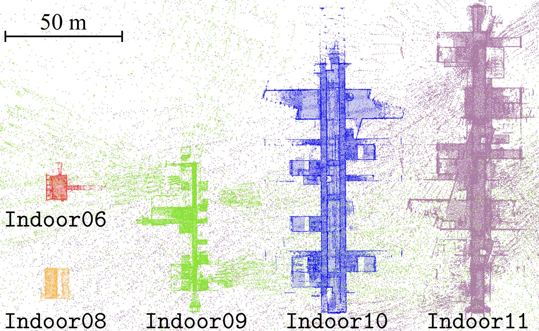
(a)

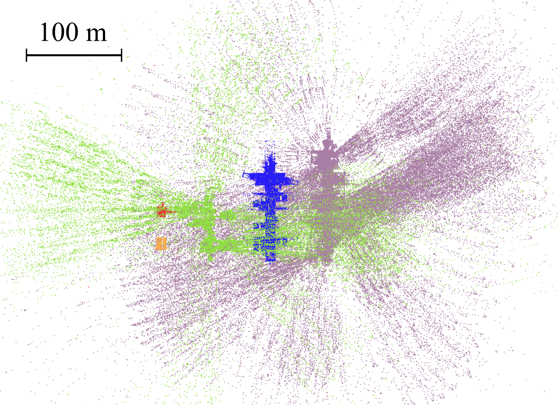
(b)

Fig. A1: Visualized map clouds of the TIERS dataset in our experiments. (a) Different scales of the sequences used in our experiments. While each scan is utilized for our evaluation, we build and then visualize map clouds using LiDAR point cloud scans and corresponding poses to illustrate the different scales of the surroundings. (b) A zoomed-out visualization of (a), highlighting the noisy characteristics inherent to indoor LiDAR scanning. Unlike RGB-D sensors, LiDAR sensors emit laser rays and calculate distance by measuring time-of-flight. However, in indoor environments, materials with high reflectivity, such as marble and glass, are highly likely to cause specular and multiple reflections. As a result, these reflections increase the time-of-flight, leading to noisy and incorrect range measurements.

C Rationale behind dataset selection

Here, we explain our detailed rationale for why we chose the aforementioned data as our comprehensive dataset.

Variation in environmental scales. First, we want to construct sufficient domain generalization between indoor and outdoor scenes. For existing approaches, only 3DMatch and KITTI were used for indoor-to-outdoor (and vice versa) evaluations. Unfortunately, these experimental setups could not assess how well the methods would perform indoors when using a non-RGB-D camera. Specifically, the maximum range was set to 5 m for 3DMatch and 80–100 m for KITTI.

However, even in indoor environments, LiDAR sensors can measure much farther, as presented in Fig. 2(b) and Fig. A1. Therefore, we aimed to challenge the bias that indoor and outdoor settings can be strictly distinguished by maximum range and decided to include TIERS. That is, in TIERS, although all sequences were collected within the same indoor building, they were captured in diverse environments such as rooms, classrooms, and hallways. As a result, the scale of the surroundings captured by the sensor varies significantly. This was intended to evaluate whether methods could still perform well on indoor scenes beyond the room level, as opposed to the conventional settings in 3DMatch. Moreover, in the TIERS, when data is acquired in a real corridor environment using LiDAR, the point cloud becomes noisy due to the diffuse reflection of laser rays; see Fig. A1(b).

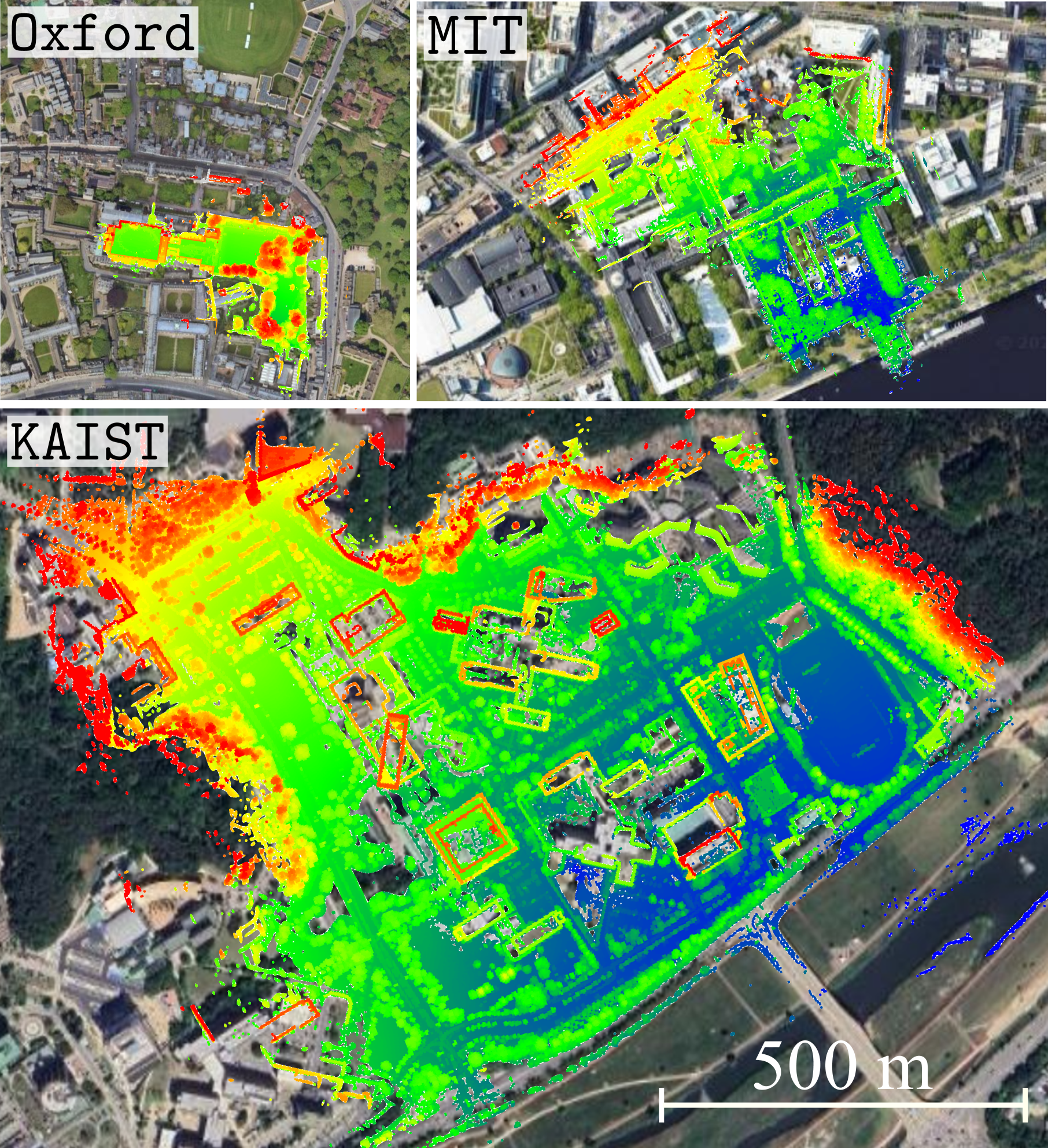
Fig. A2: Scale comparison of three sequences: Oxford from the NewerCollege [61], MIT from the Kimera-Multi [71], and KAIST from the HeLiPR dataset [34] at the same scale (i.e., 500 m). Note that although these sequences fall under the same campus category, their scales differ. For clarity, the map clouds are visualized with respect to their $z$ values.

Likewise, one might think that the scales of campus environments are similar; however, as shown in Fig. A2, even within the campus category, variations in campus size can lead to differences in the distribution of LiDAR sensor data. Therefore, by incorporating datasets with varying environmental scales, we aim to ensure that our generalizability benchmark includes the full spectrum of scale variations, enabling a more comprehensive assessment of generalization across different settings.

Different scanning patterns with different sensor types. In addition to using the TIERS for the reasons mentioned above, we also aimed to evaluate whether the same space remains robust to different scanning patterns. To this end, we employed KAIST and TIERS. As shown in Fig. A3, even when the same space is captured, variations in the number of laser rays and sensor patterns result in different representations.

Acquisition setups.   We also considered that acquisition setups vary in multiple ways. A common bias in previous evaluations in the state-of-the-art approaches is that indoor scanning is performed using handheld devices, whereas outdoor scanning is conducted using vehicles (i.e., the assumption that indoor scanning is performed using a handheld setup, while outdoor scanning is conducted using a vehicle). Thus, we aimed to evaluate whether registration remains robust to different acquisition setups to challenge this assumption. For this reason, we included TIERS, which was acquired using a sensor cart, and Oxford, which was acquired using both a handheld device and a quadruped robot.

Additionally, MIT was captured using a mobile robot, which performs planar motion similar to a vehicle. However, due to its smaller size, the robot’s body experiences significantly more roll and pitch motion, potentially introducing greater motion noise compared to a vehicle.

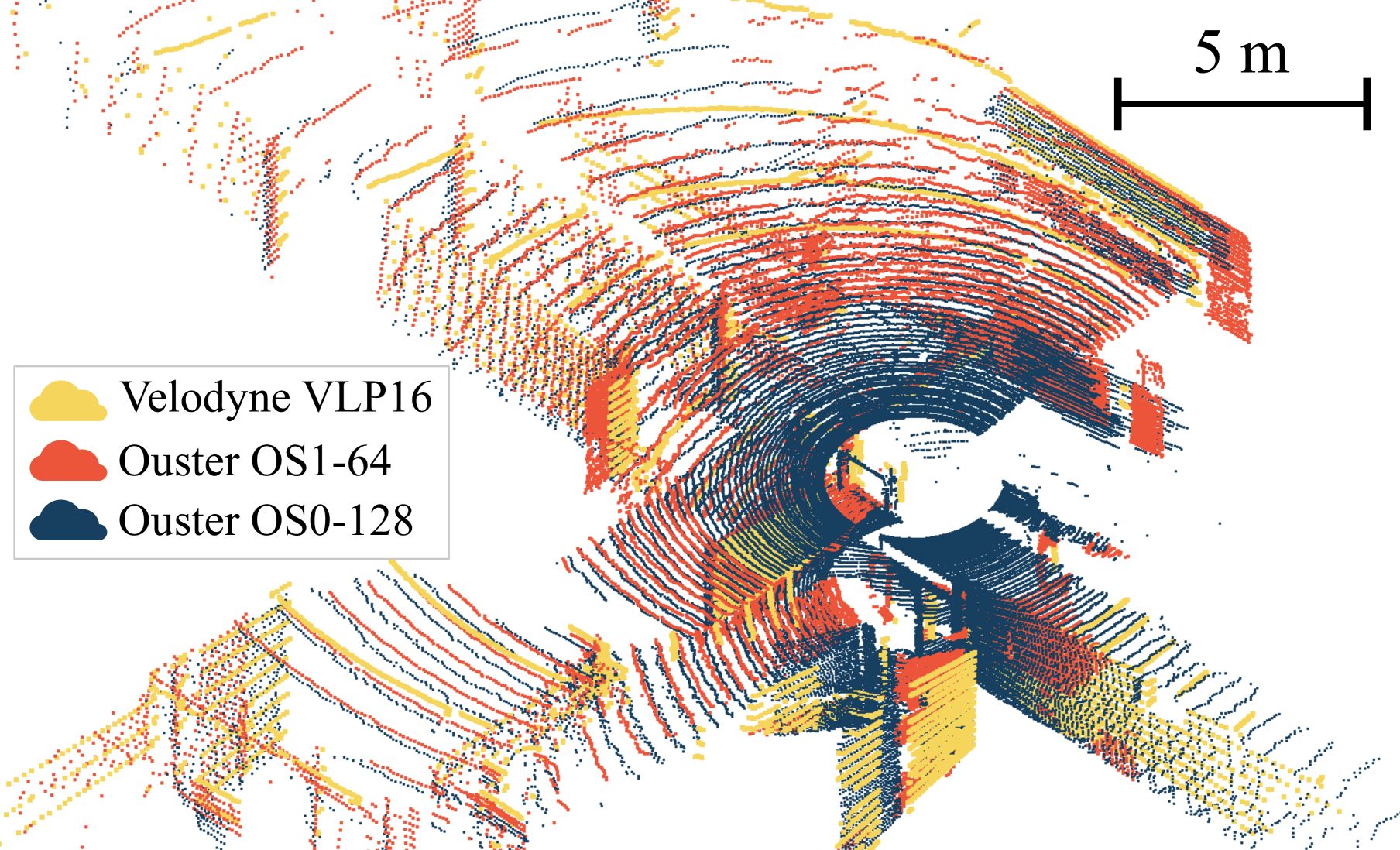
(a)

(b)

Fig. A3: Examples of visualized LiDAR scans from different LiDAR sensors in (a) the Indoor10 of TIERS dataset [60] and (b) KAIST05 sequence of the HeLiPR dataset [34]. Note that even in the same environment, differences in the number of LiDAR rays and field of view result in point clouds with different patterns.

Diversity of geographic and cultural environments. Lastly, we also aimed to assess whether the acquired data could be generalized across geographic and cultural differences. Some studies [13] have claimed that training on KITTI and testing on KITTI-360 could demonstrate domain generalization. However, since both datasets were collected in Germany using the same vehicle platform, they fall short of demonstrating actual cultural differences.

To address this issue, we leveraged datasets collected from campuses in Asia, Europe, and the USA to evaluate whether such geographic and cultural variations could be accounted for in our proposed benchmark.

D Trade-off between generalization and robustness against partial overlaps

Here, as a supplement to the explanation in Sec. 5.4, we explain with an example why our methodology performed relatively poorly on 3DLoMatch in detail [32]. Suppose we have two arbitrary L-shaped point clouds, as presented in Fig. A4(a). Then, these two L-shaped point clouds can be registered in the following cases:

• Case A: overlapped along the longer segment (Fig. A4(b))

• Case B: overlapped in the short direction (Fig. A4(c))

• Case C: fully overlapped (Fig. A4(d)).

Obviously, the lowest value of the loss function is the fully overlapped case (i.e., Case C); however, in the partial overlap problem, the other local optima (i.e., the partially overlapped case along the longer or shorter segment) can be the actual global optimum. This phenomenon implies that when partial overlap is severe, the relative pose with the smallest loss value is not necessarily the true global optimum.

Therefore, in terms of the optimization problem, we can say that the state with the actual global optimum is not necessarily equal to the state with the global optimum in the cost function. Furthermore, this problem cannot be solved mathematically without prior knowledge of how the two point clouds should be aligned. We refer to this phenomenon as global optimum ambiguity.

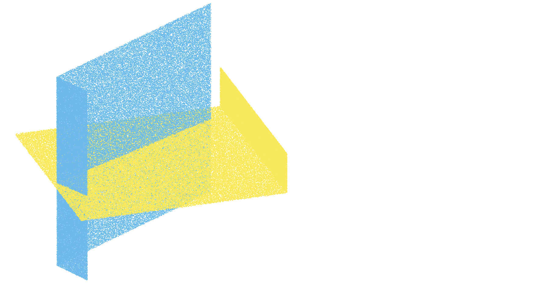
(a)

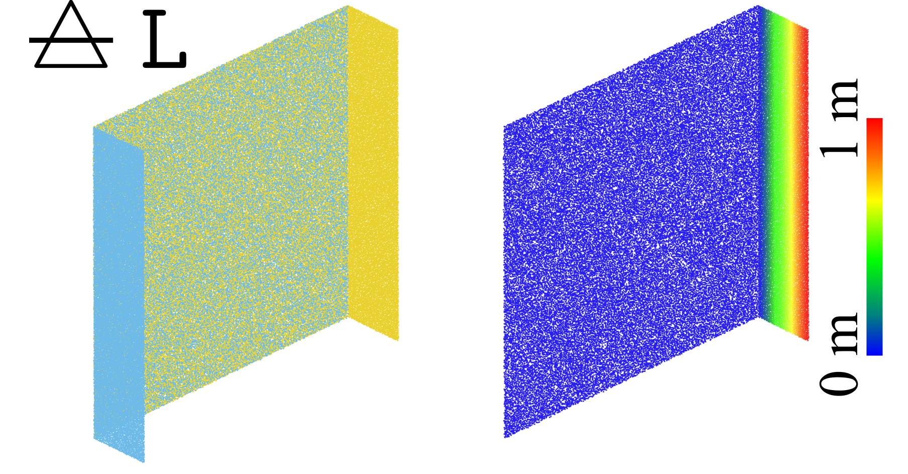
(b)

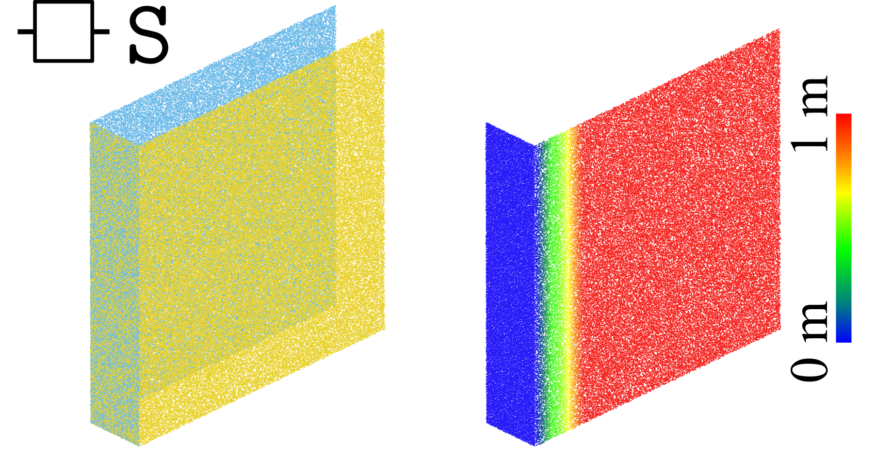
(c)

(d)

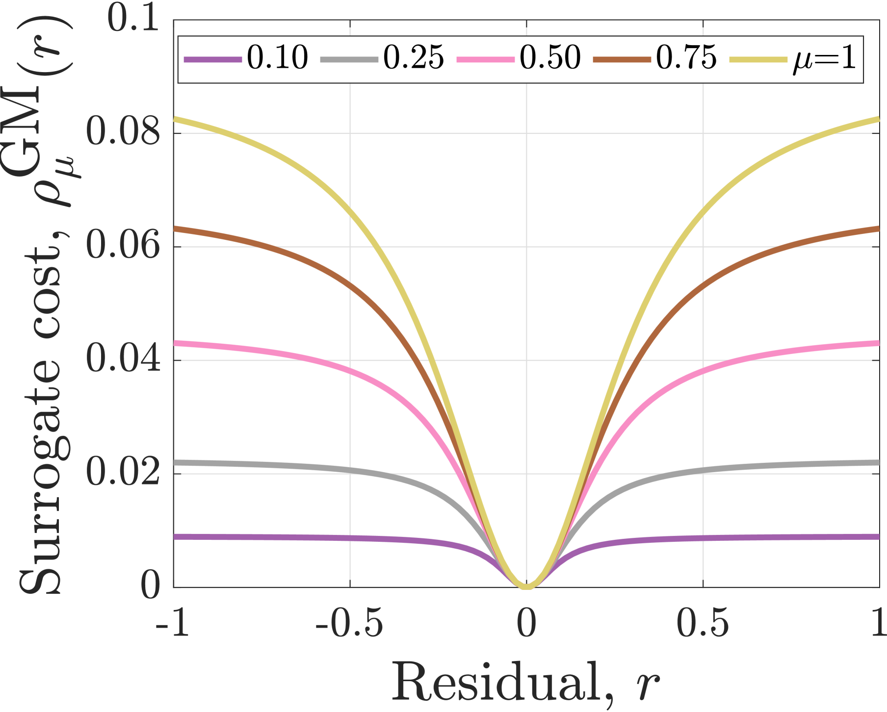
(e)

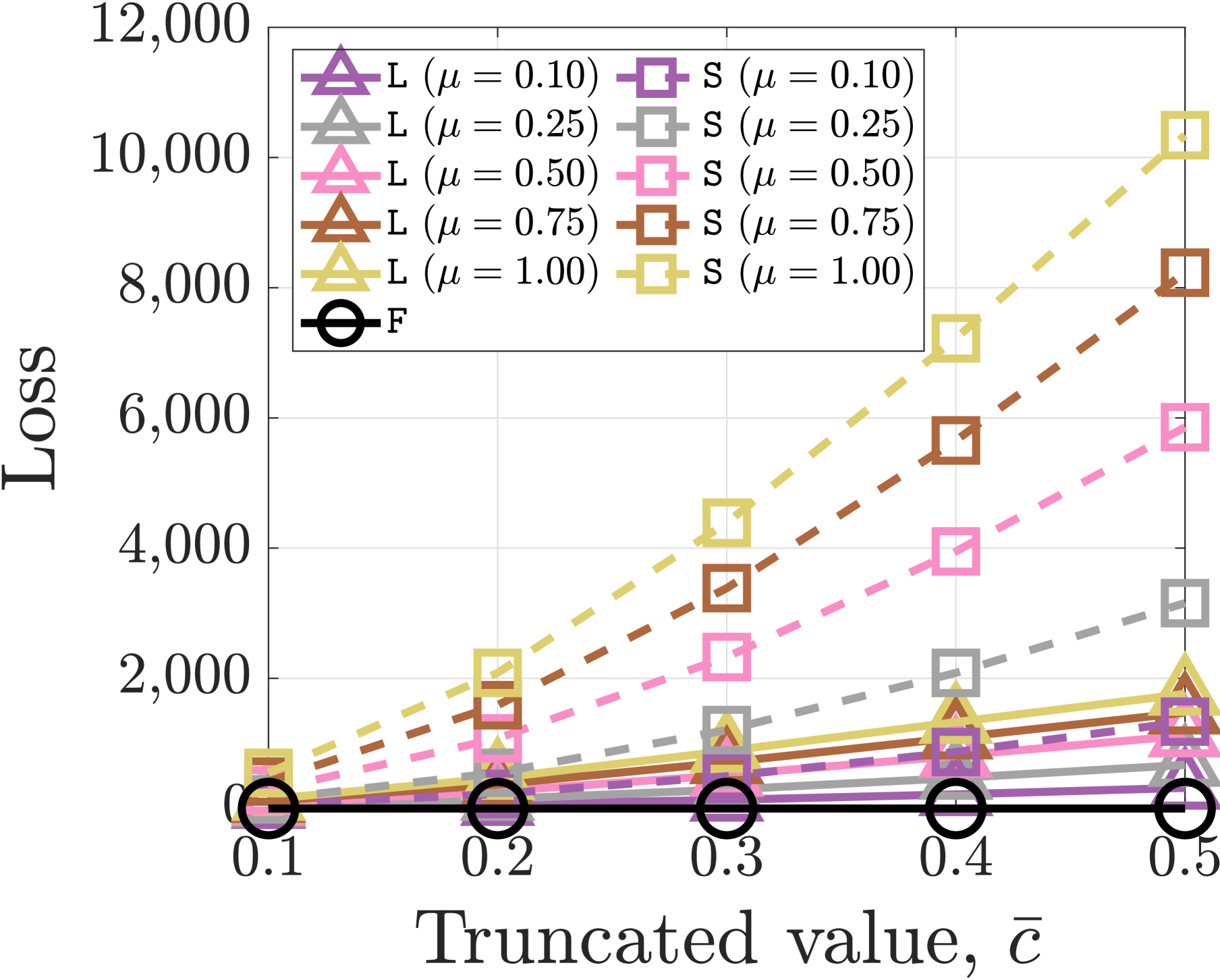
(f)

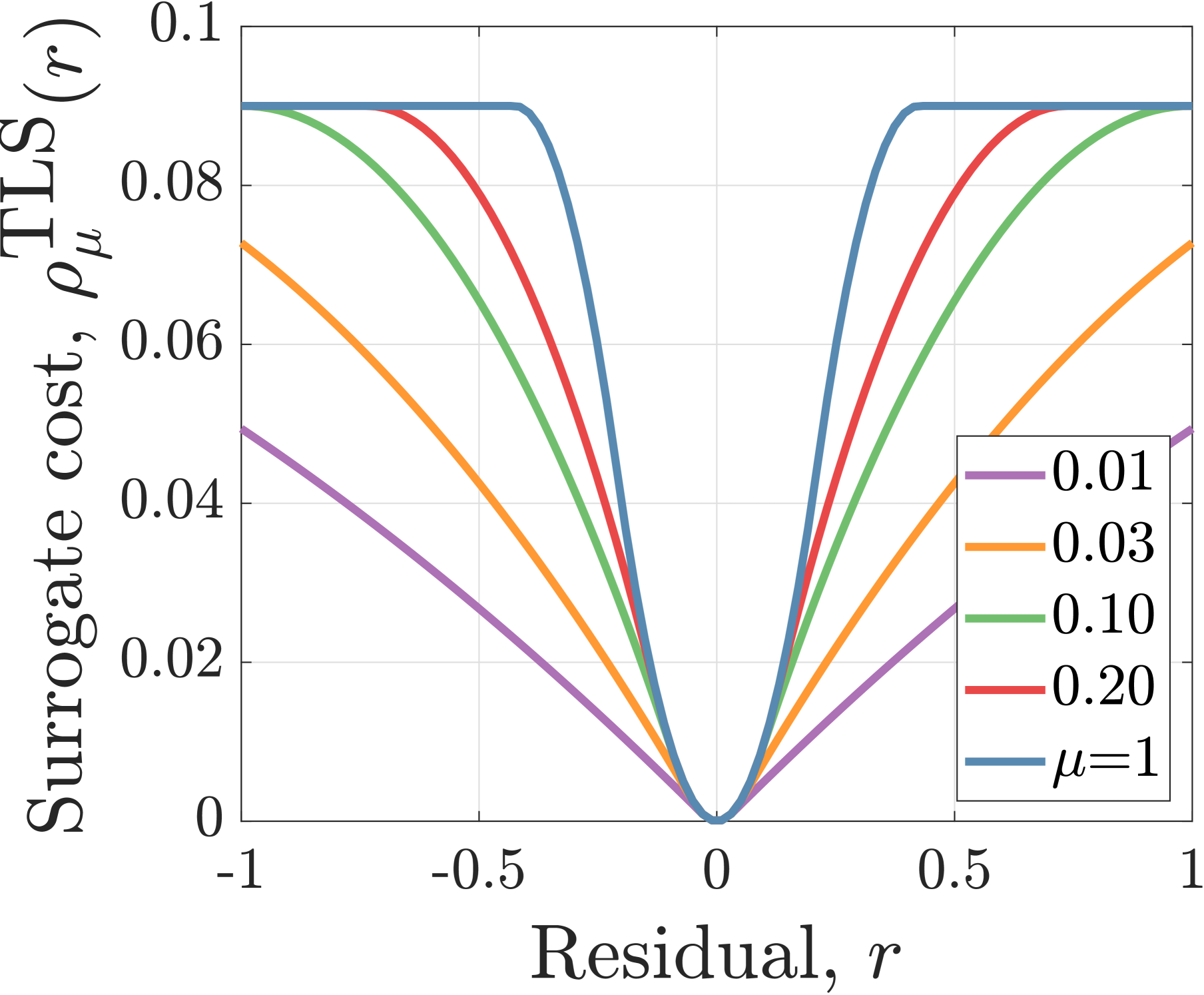
(g)

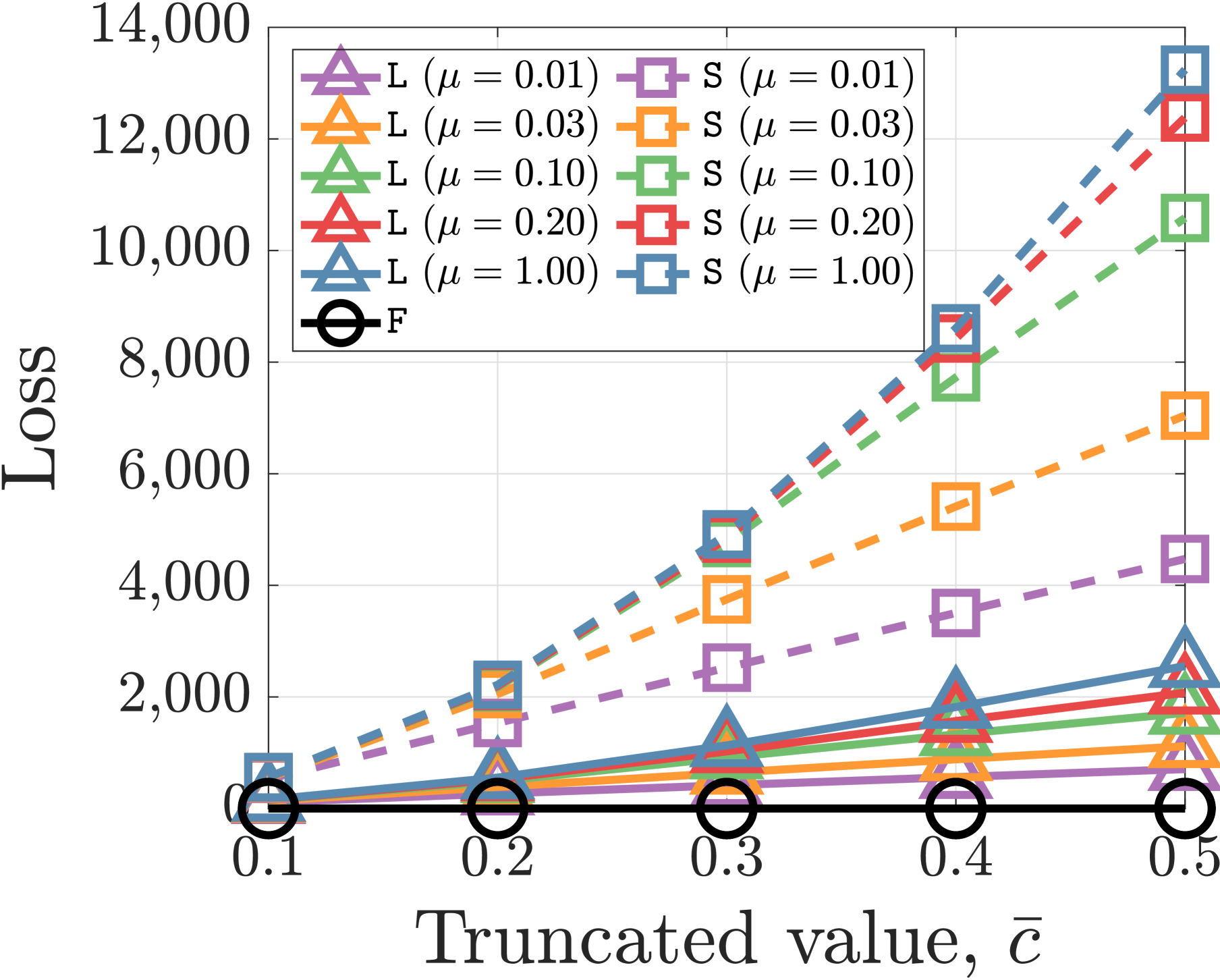
(h)

Fig. A4: Illustration of the global optimum ambiguity problem in point cloud registration. (a) Example of two misaligned L-shaped point clouds and (b)–(d) possible registration cases. (b) An overlapped case along the longer segment (expressed as L), (c) an overlapped case along the shorter segment (expressed as S), and (d) a fully overlapped case (expressed as F). (e) The behavior of the surrogate cost function of German-McClure (GM) with varying control parameter $\mu$ and (f) corresponding loss values for various $\mu$ with the user-defined threshold parameter $\bar{c}$. (g) The behavior of the surrogate cost function of truncated least squares (TLS) with $\mu$ and (f) corresponding loss values for various $\mu$ with the user-defined threshold parameter $\bar{c}$. Note that, regardless of the given $\mu$ and $\bar{c}$, the fully overlapped case (i.e., (d)) always results in the lowest loss (since the loss value is zero for any $\mu$ and $\bar{c}$, for simplicity, only a single F is presented in (f) and (h)).

In addition, even with a learnable non-linear robust kernel, this problem cannot be perfectly resolved. For instance, we examine two renowned non-convex cost functions: a) German-McClure (GM) function and b) truncated least squares (TLS) function, and use them as surrogate cost functions $\rho_{\mu}(r)$ that adjust their non-linearity by changing the control parameter $\mu$ [75]. Formally, by letting the $r$ be the residual and $\bar{c}$ be the user-defined parameter that determines the shape of a kernel, the GM function with $\mu$ can be expressed as follows:

$$\rho^{\text{GM}}_{\mu}(r)=\frac{\mu\bar{c}^{2}r^{2}}{\mu\bar{c}^{2}+r^{2}},$$ (A12)

and the TLS function with $\mu$ can be expressed as follows:

As shown in Fig. A4, even if we vary the non-linearity of the kernel by adjusting the shape of the surrogate cost via $\mu$; see Figs. A4(e) and (g), the fully overlapped case still yields the lowest loss; see Figs. A4(f) and (h). This supports our claim that the global optimum ambiguity problem cannot be easily resolved, no matter how much we formulate it as a non-linear function.

E Qualitative results in diverse scenes

We present the quantitative results in Fig. A5 and Fig. A6. Remarkably, even when trained on 3DMatch, which consists solely of RGB-D point clouds with an approximate maximum range of 3.5 m, the model performs robustly on sparse LiDAR point clouds in both indoor and outdoor environments. In particular, our approach successfully performed registration regardless of the sensor type or acquisition setup, whether the sparse 3D point clouds were acquired by solid-state LiDAR sensors (the first row among the KAIST rows in Fig. A6) or captured from a robot platform (MIT rows in Fig. A6).

ScanNet++i
ScanNet++F
TIERS

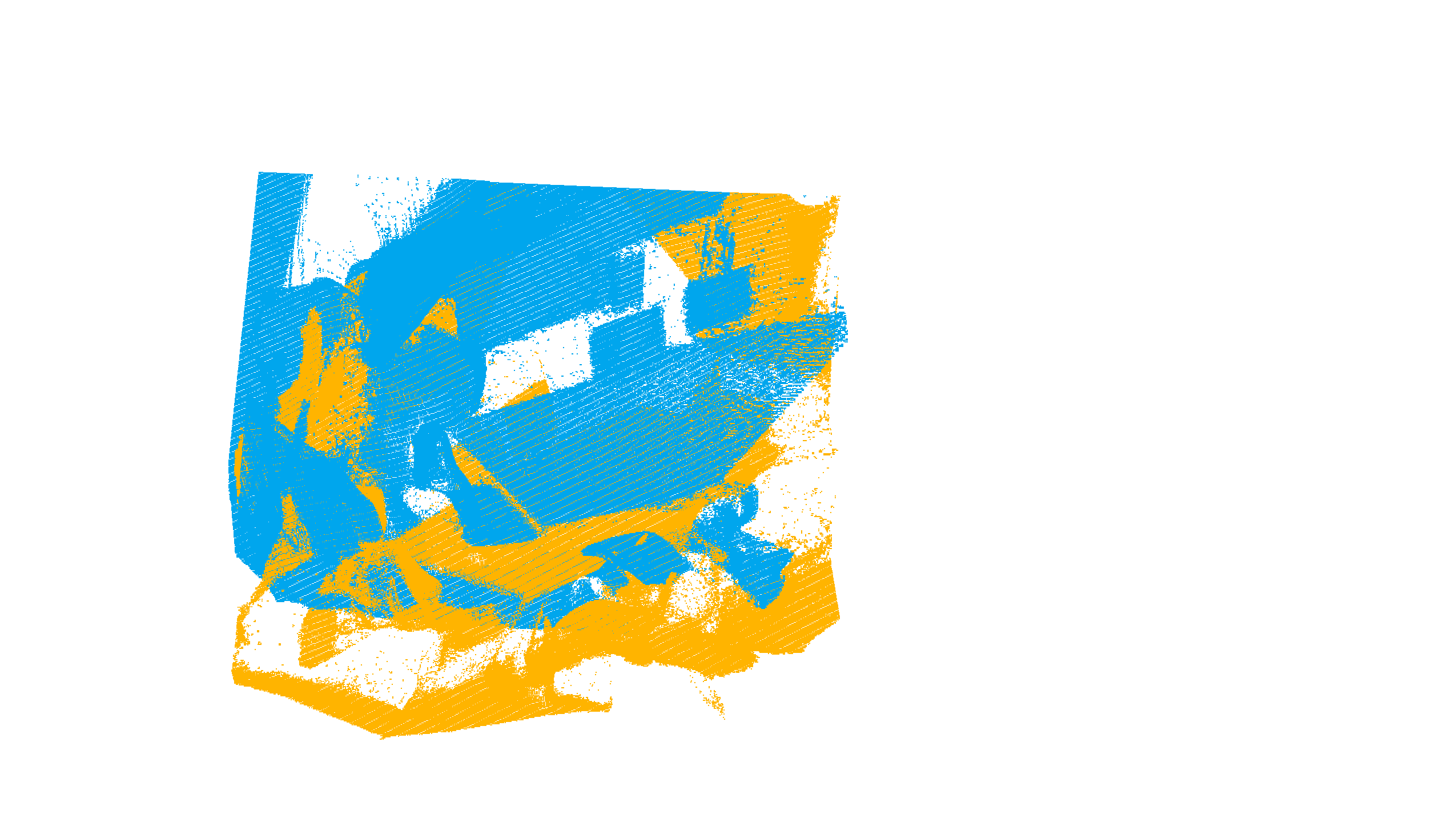
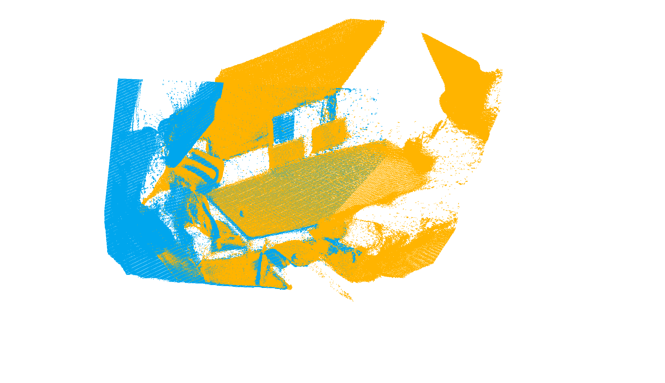
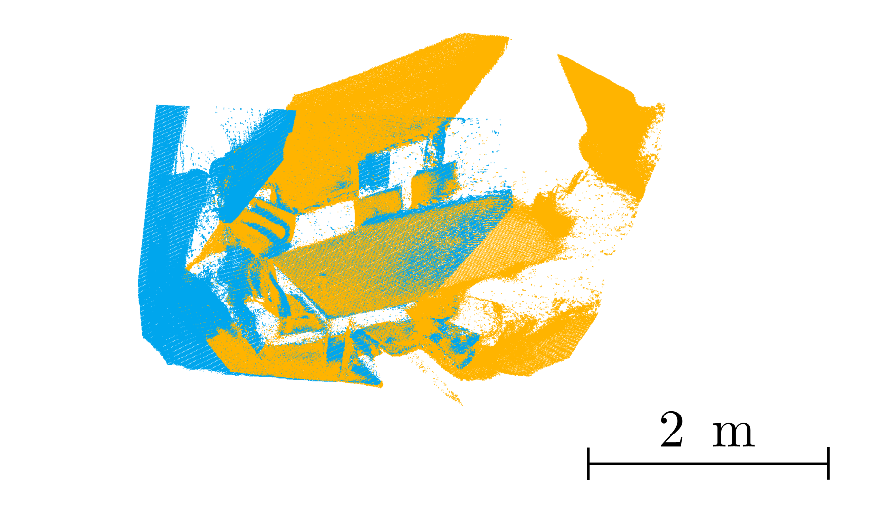
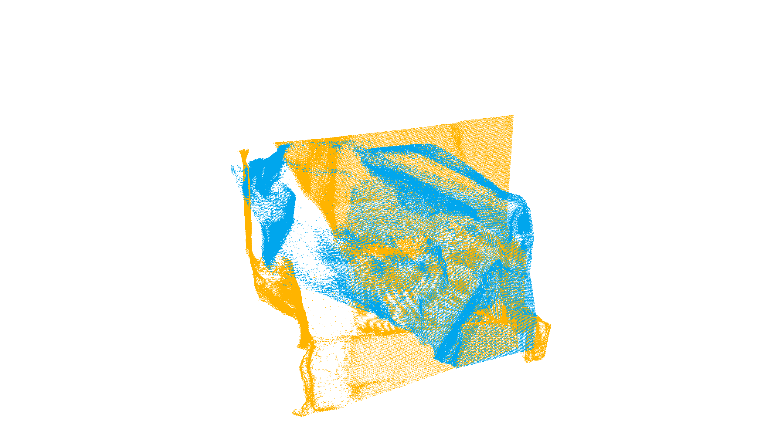
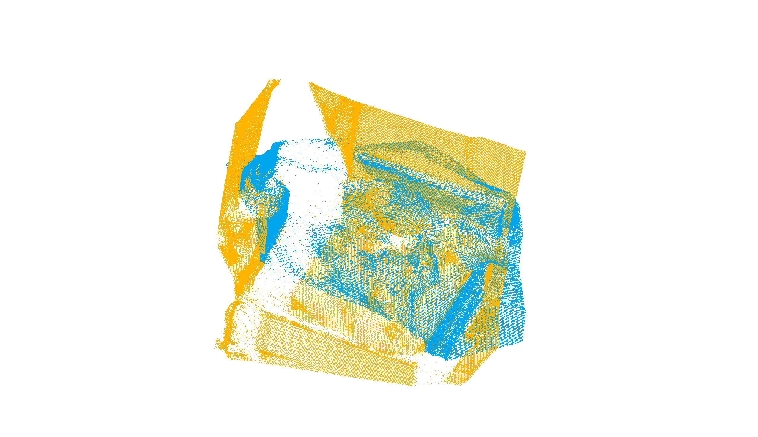
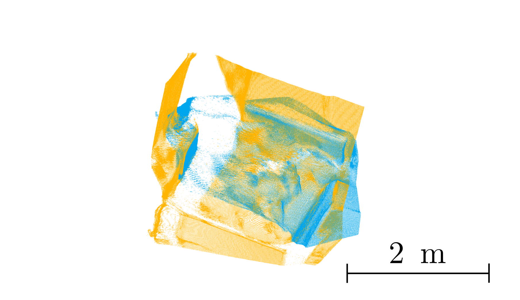
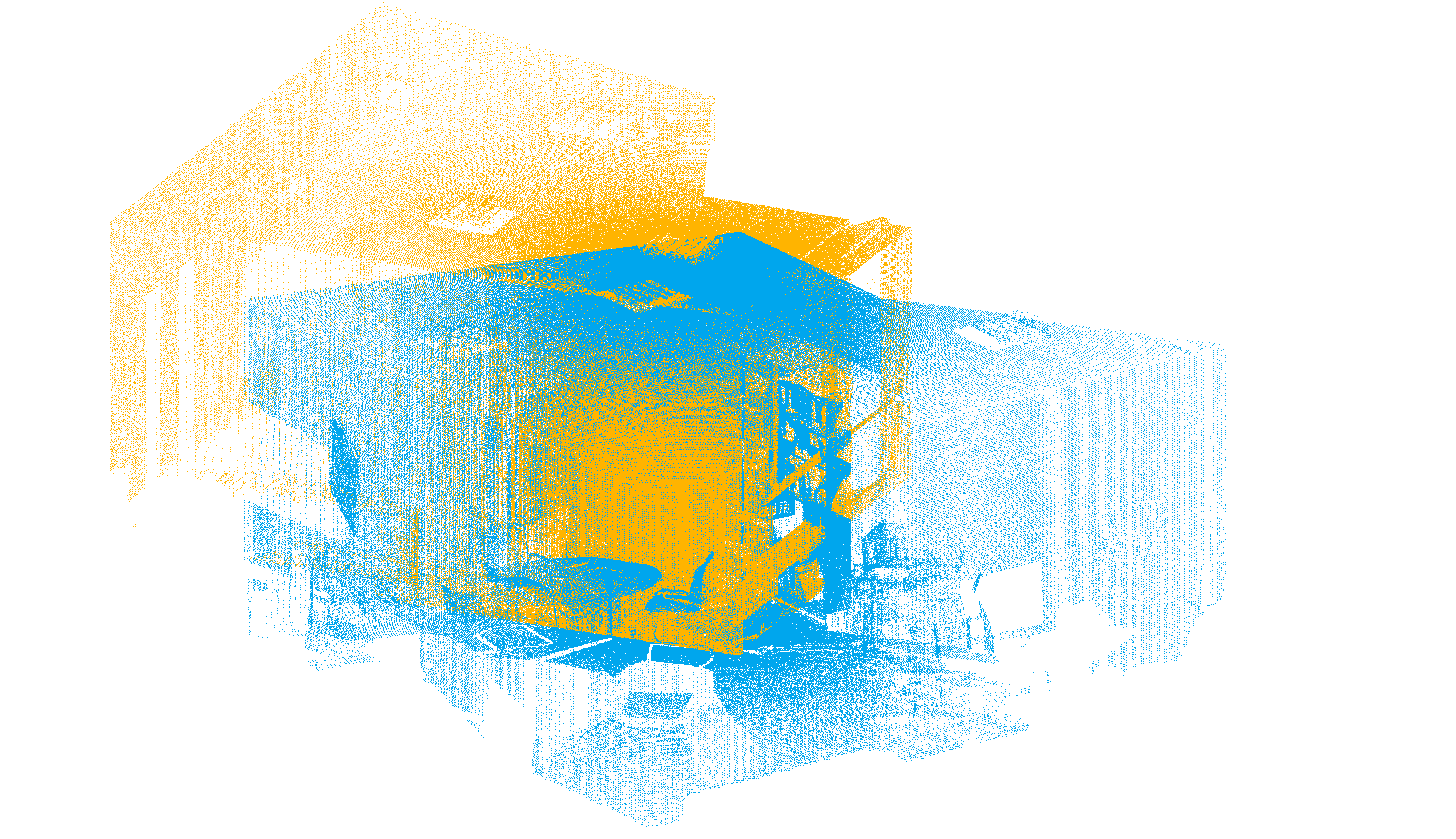
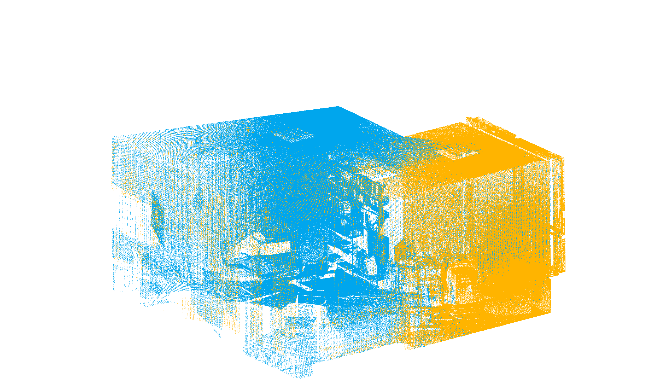
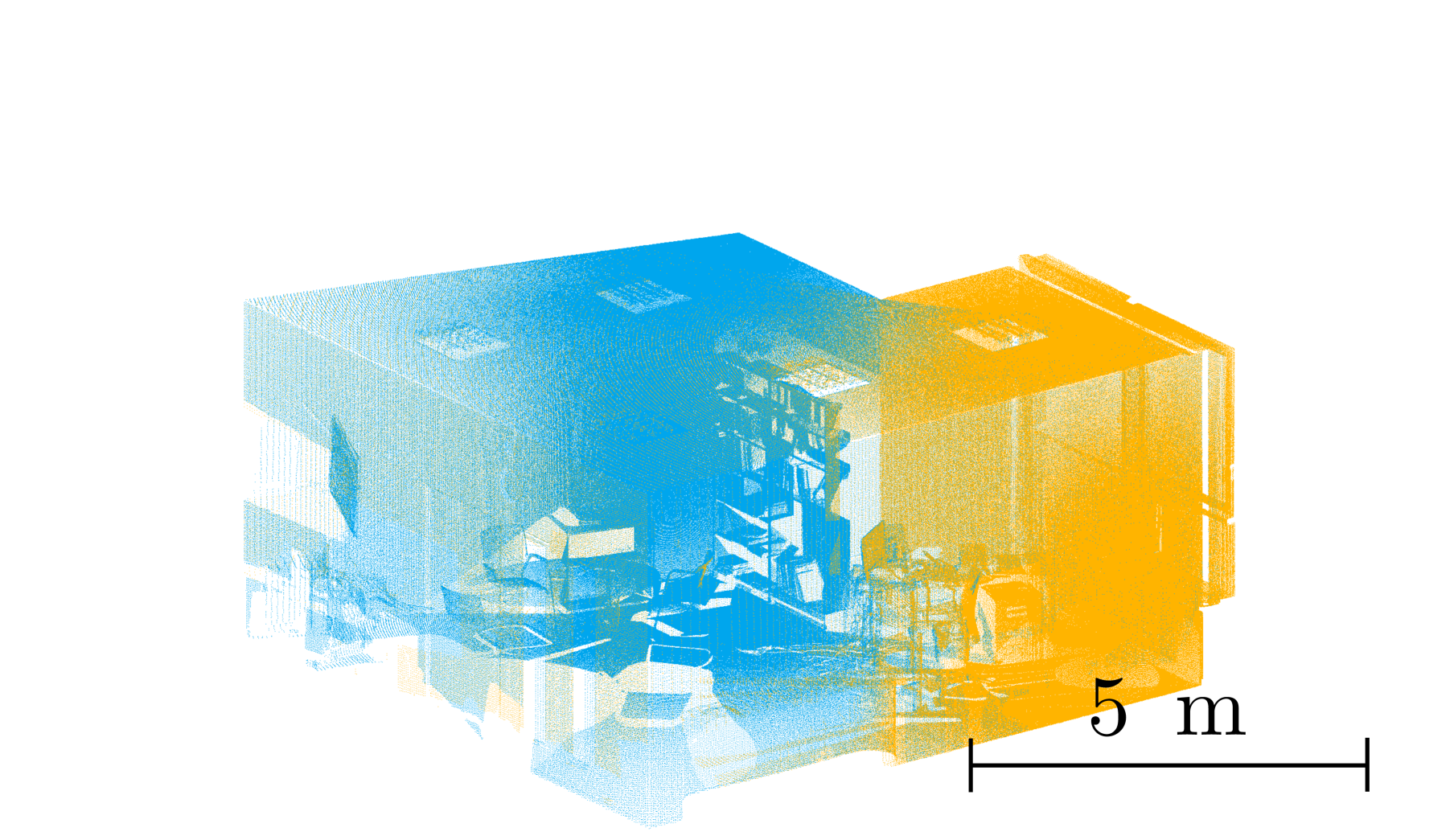
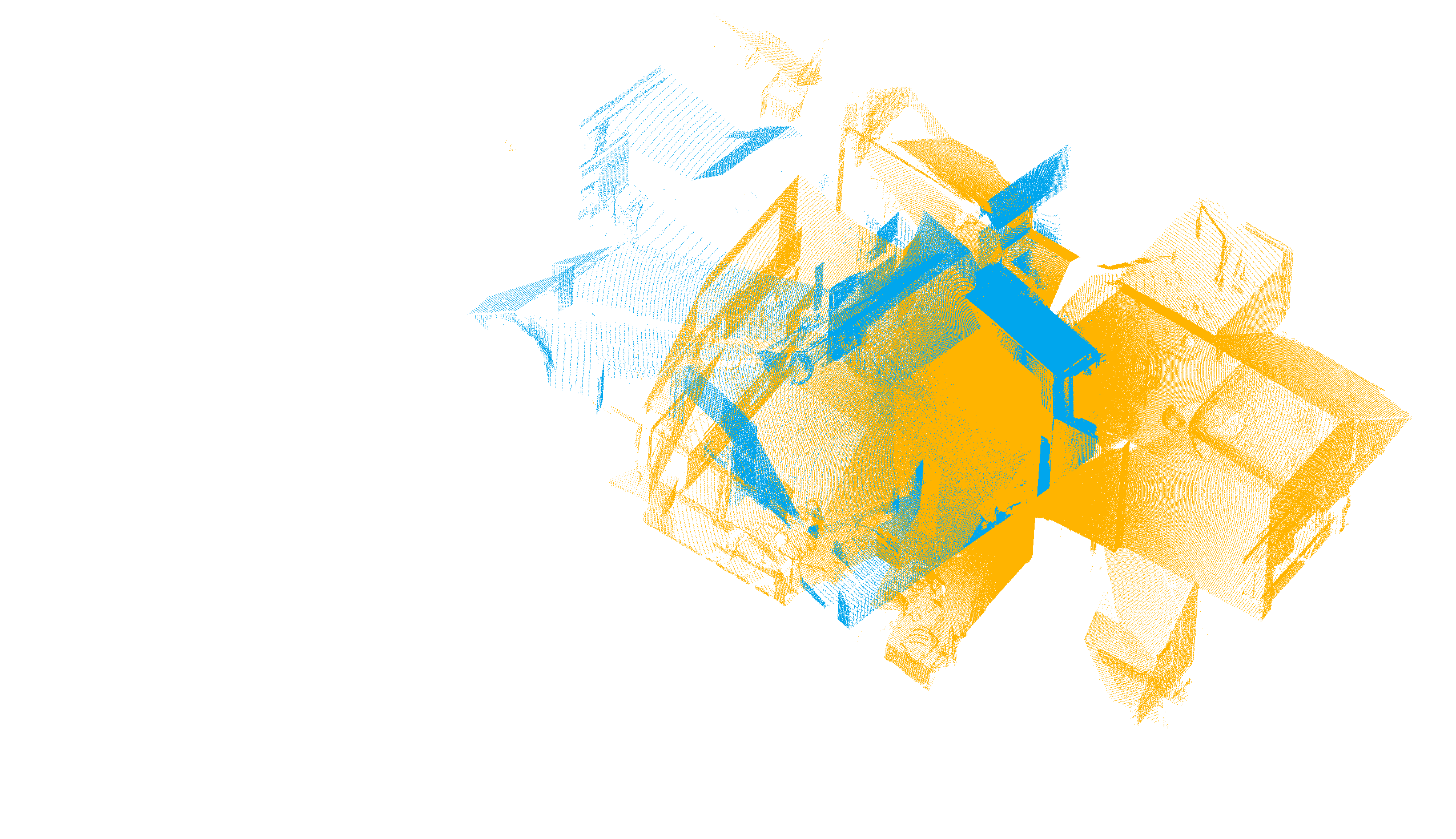
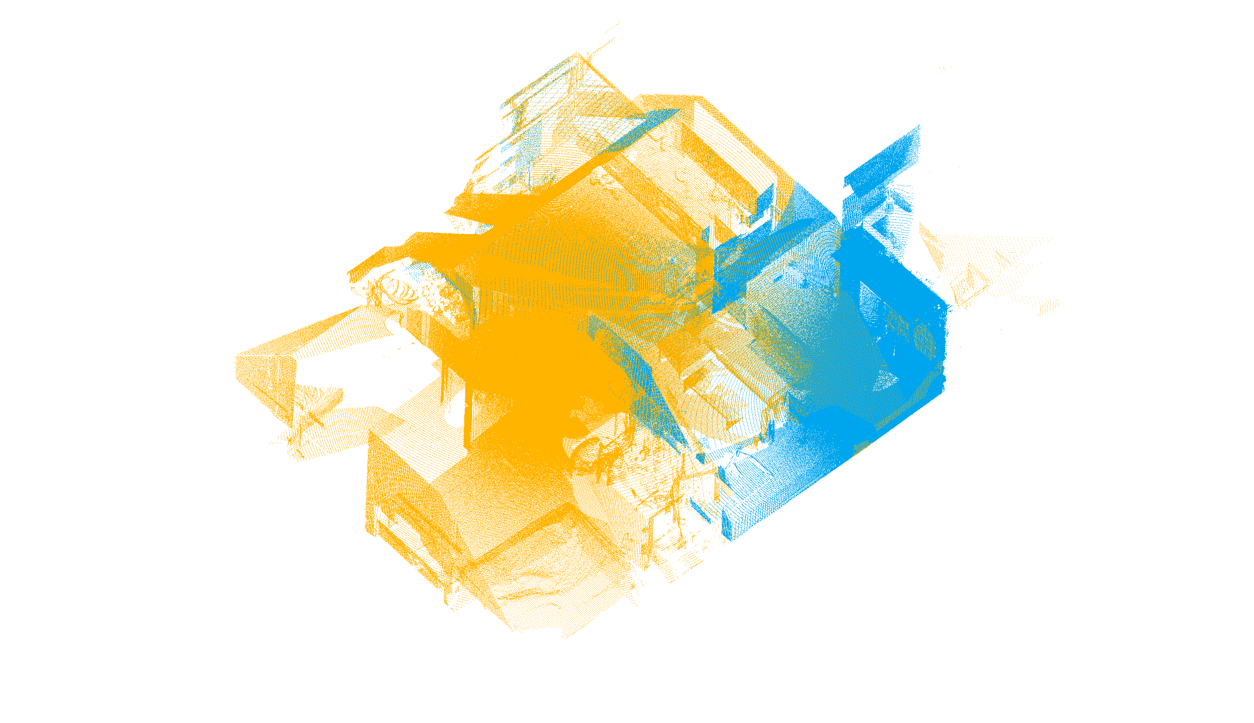
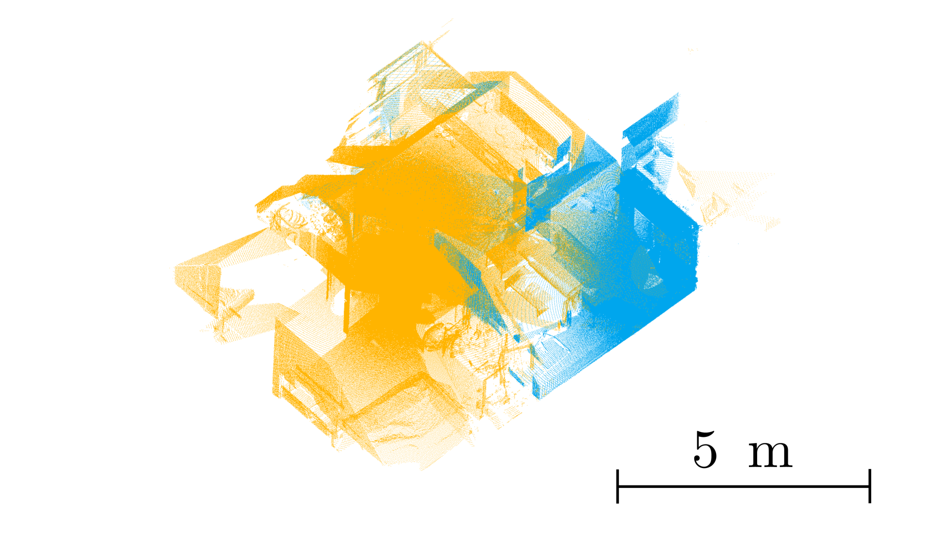
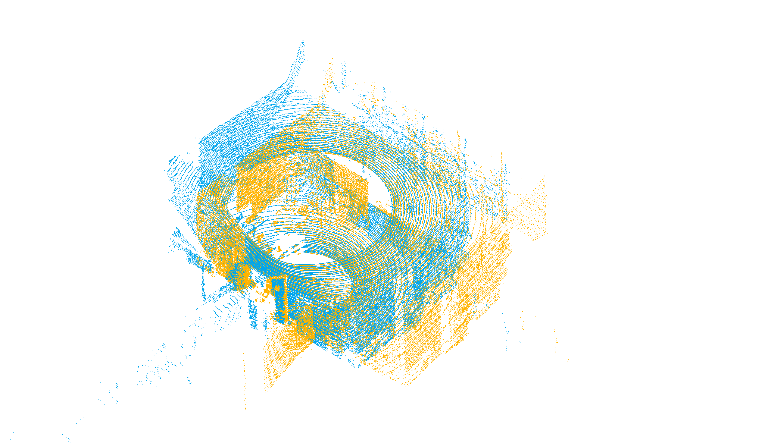
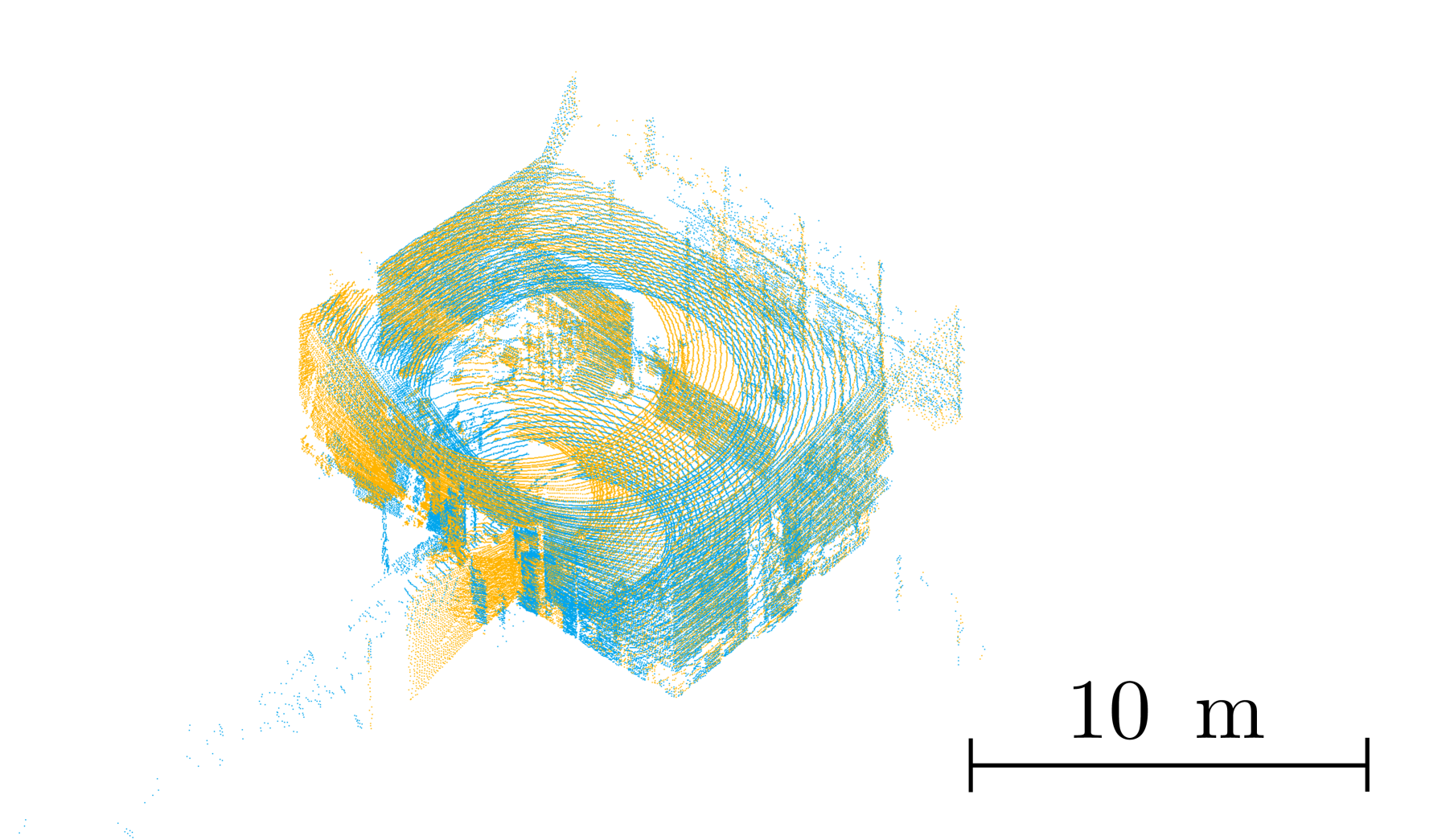
(a) Source and target

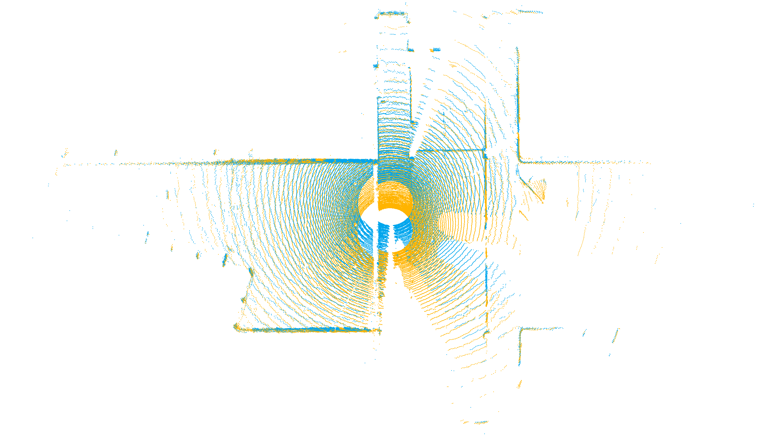
(b) BUFFER-X (Ours)

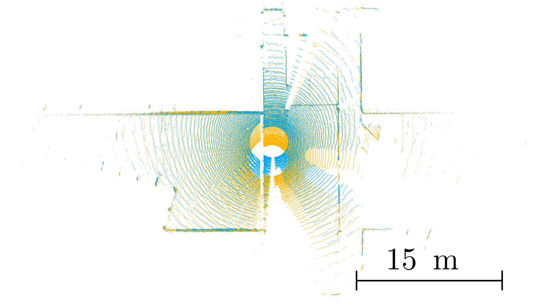
(c) Ground truth

Fig. A5: Qualitative results on indoor point cloud registration (T-B): ScanNet++i, ScanNet++F, and TIERS sequences. (a) Input source (yellow) and target (cyan) point clouds before registration. (b) Registration results obtained using our BUFFER-X. (c) Ground truth alignment. Visualization demonstrates that BUFFER-X achieves accurate alignment, closely matching the ground truth.

Oxford
KAIST
MIT

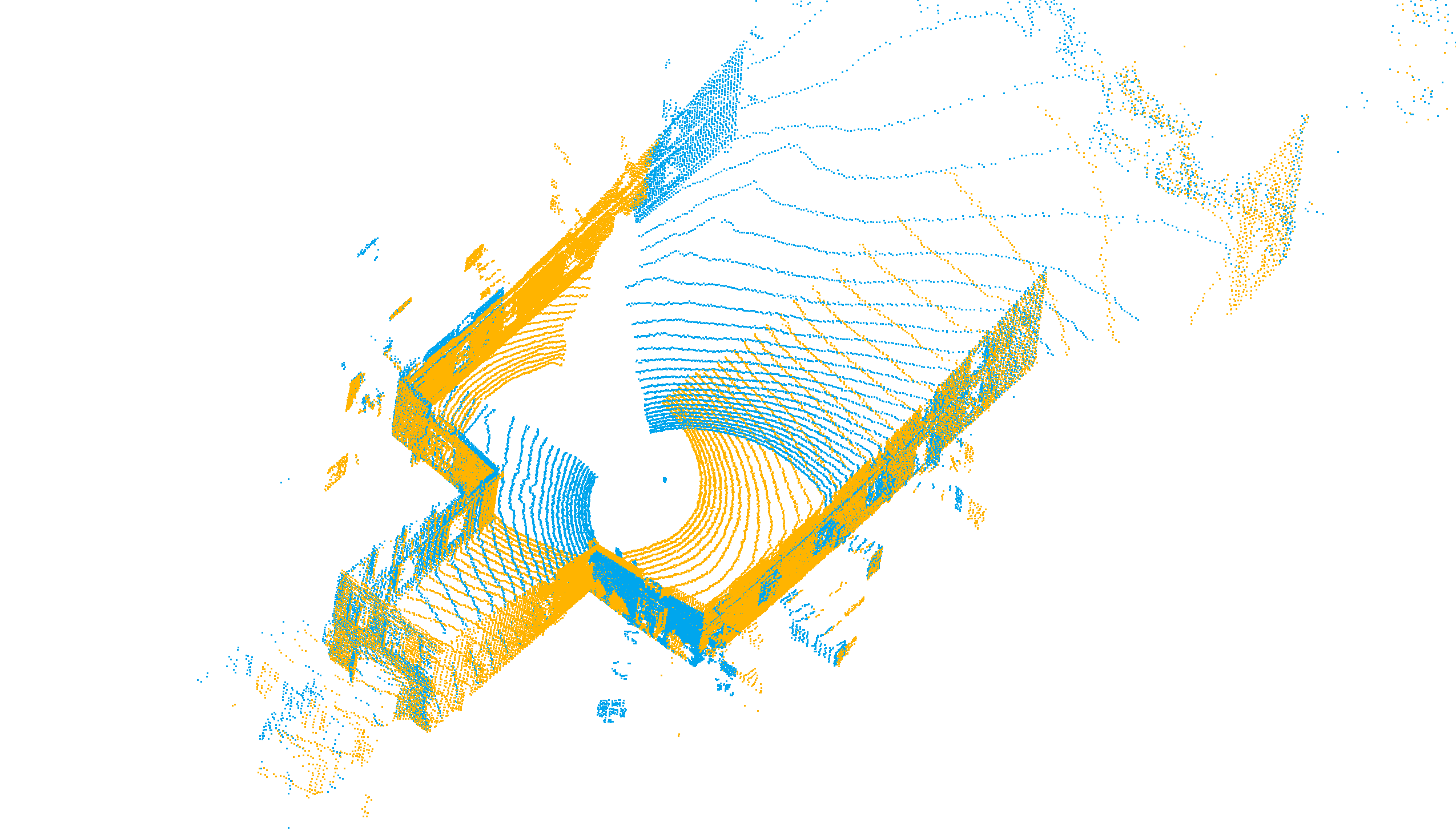
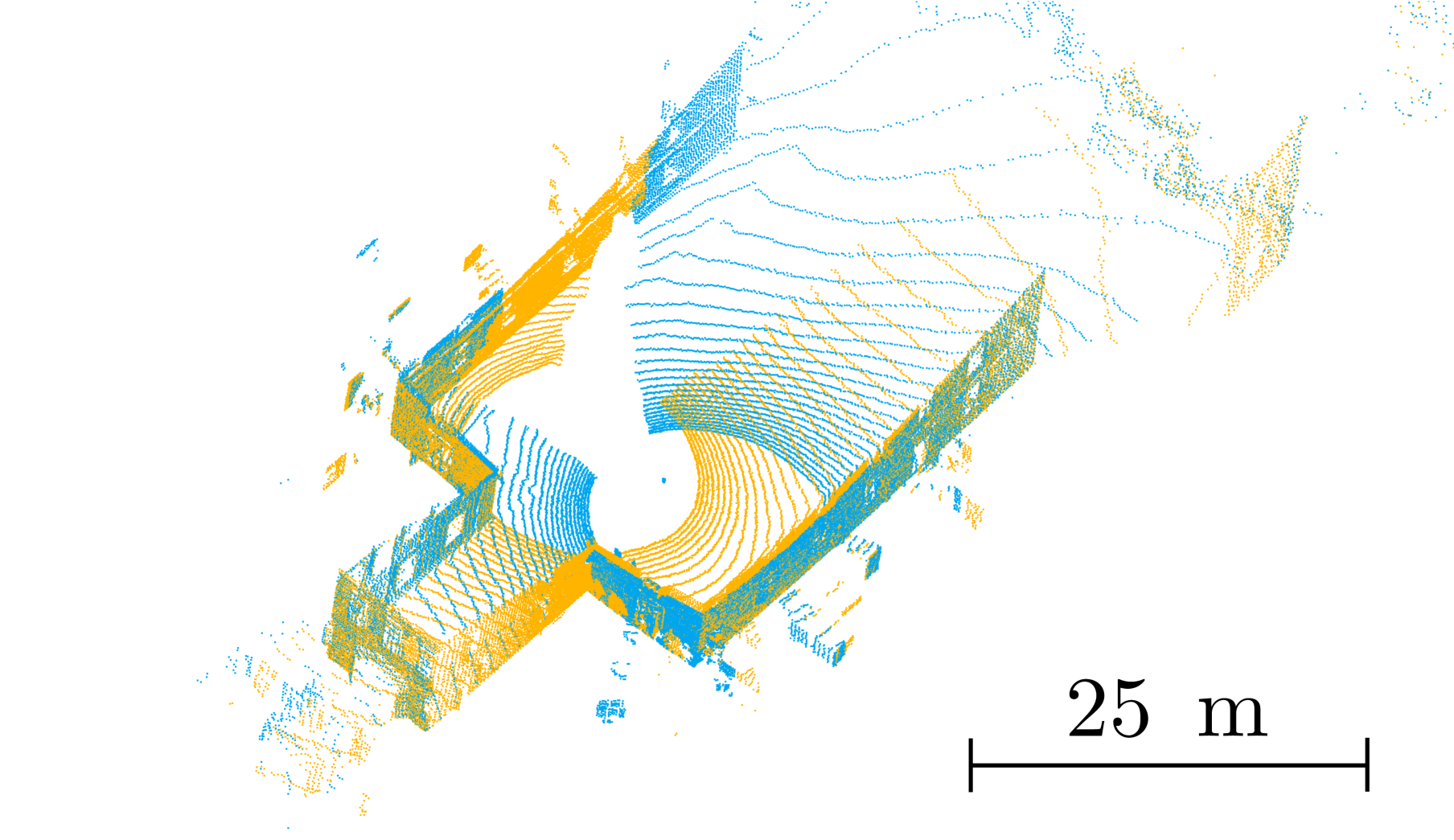
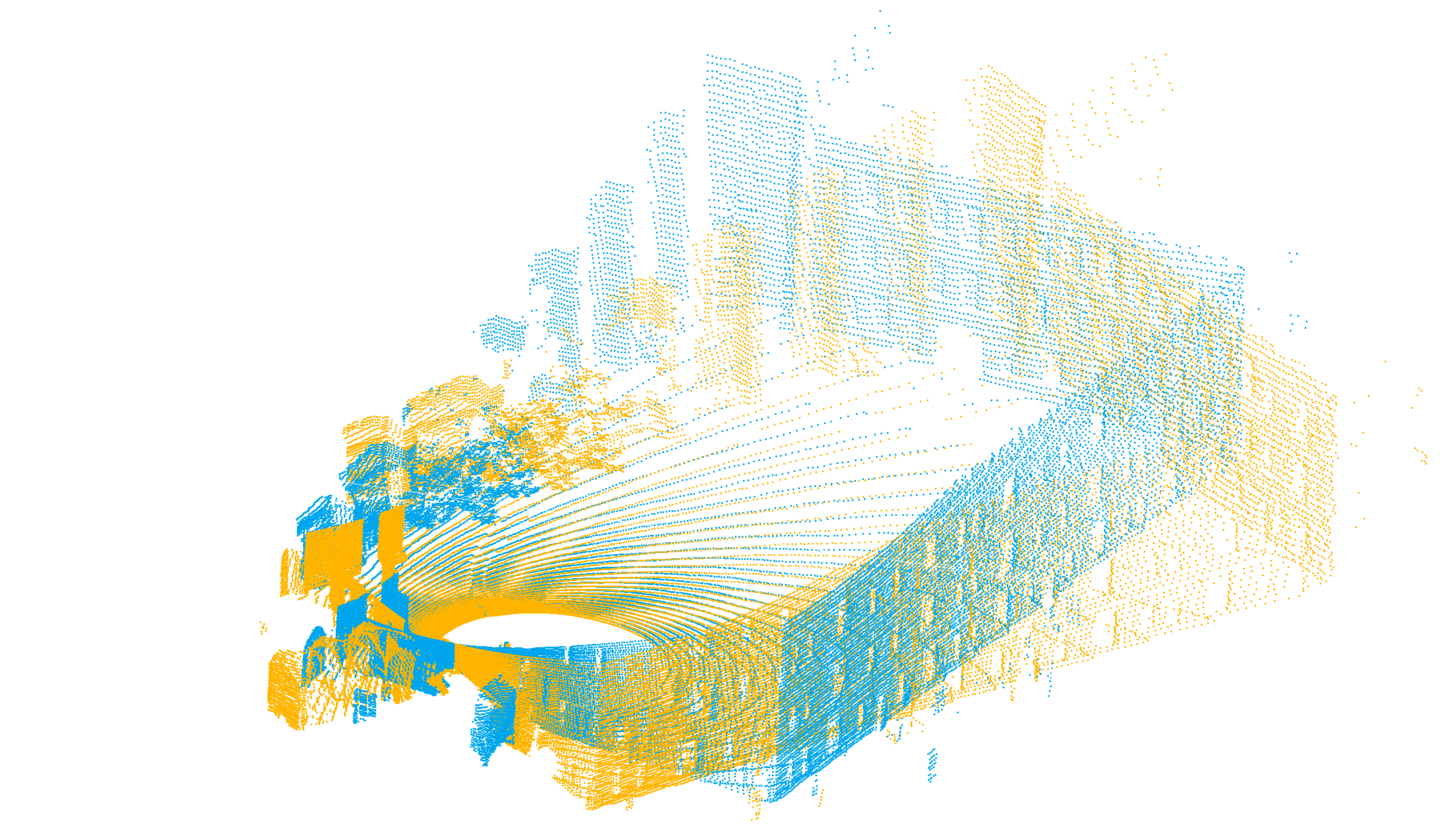
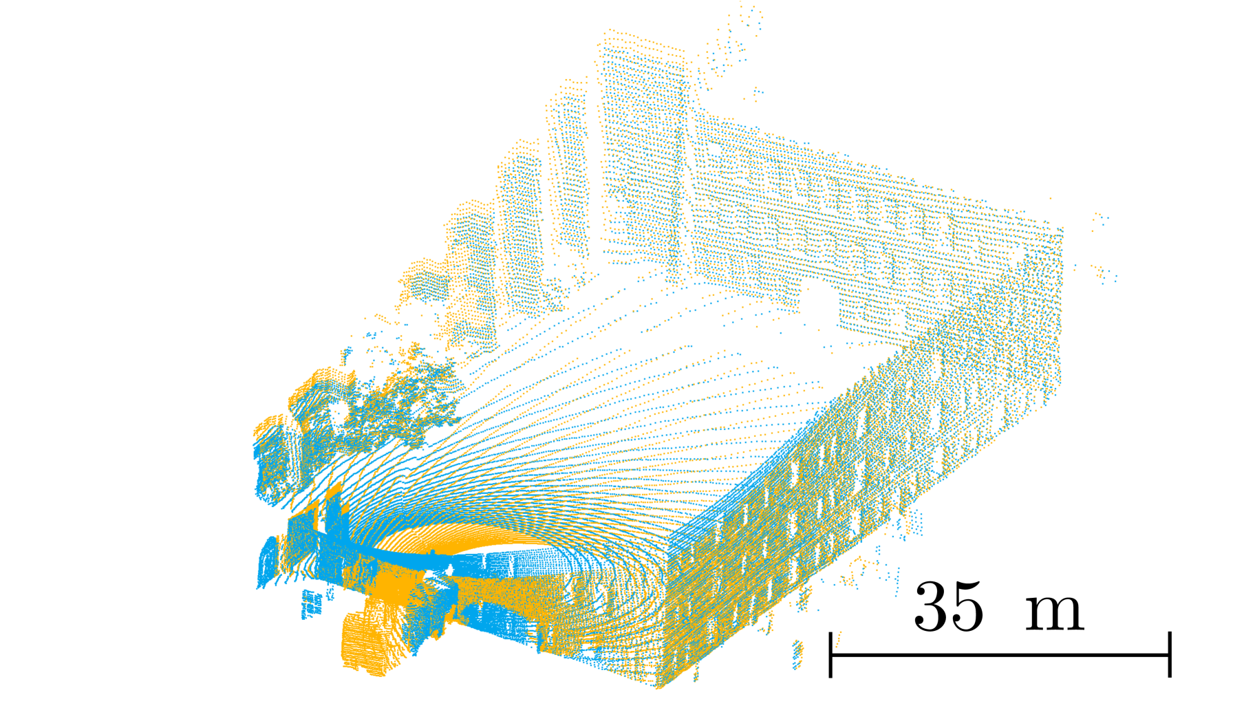
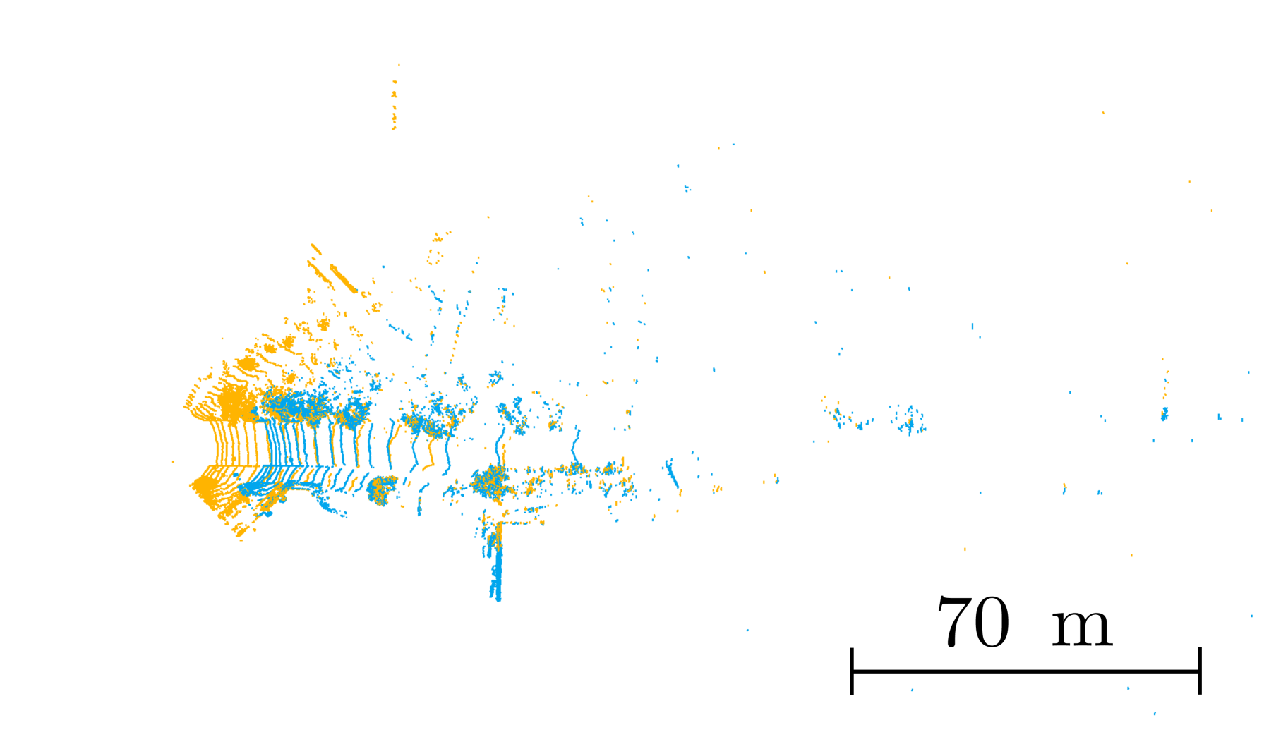
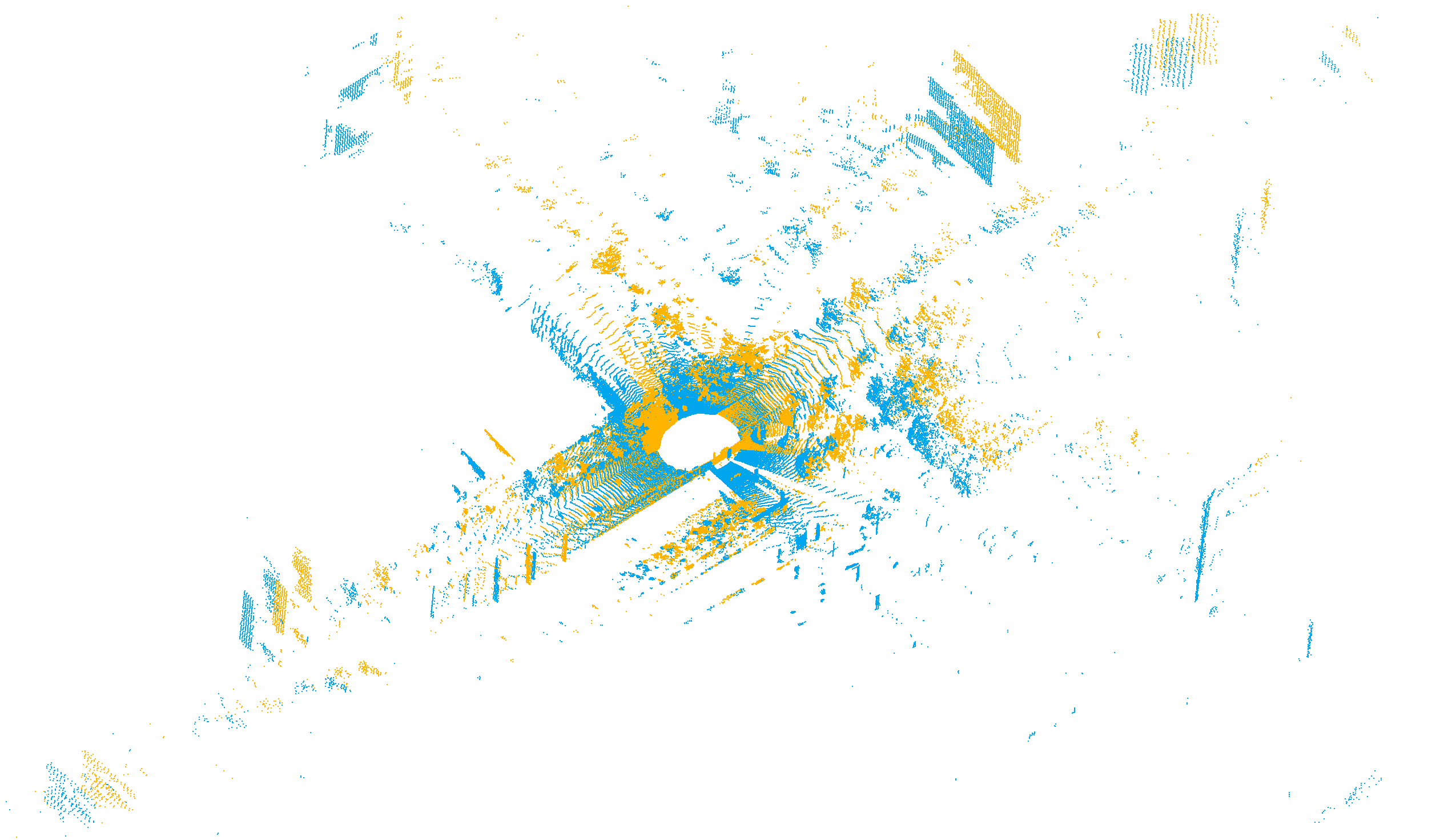
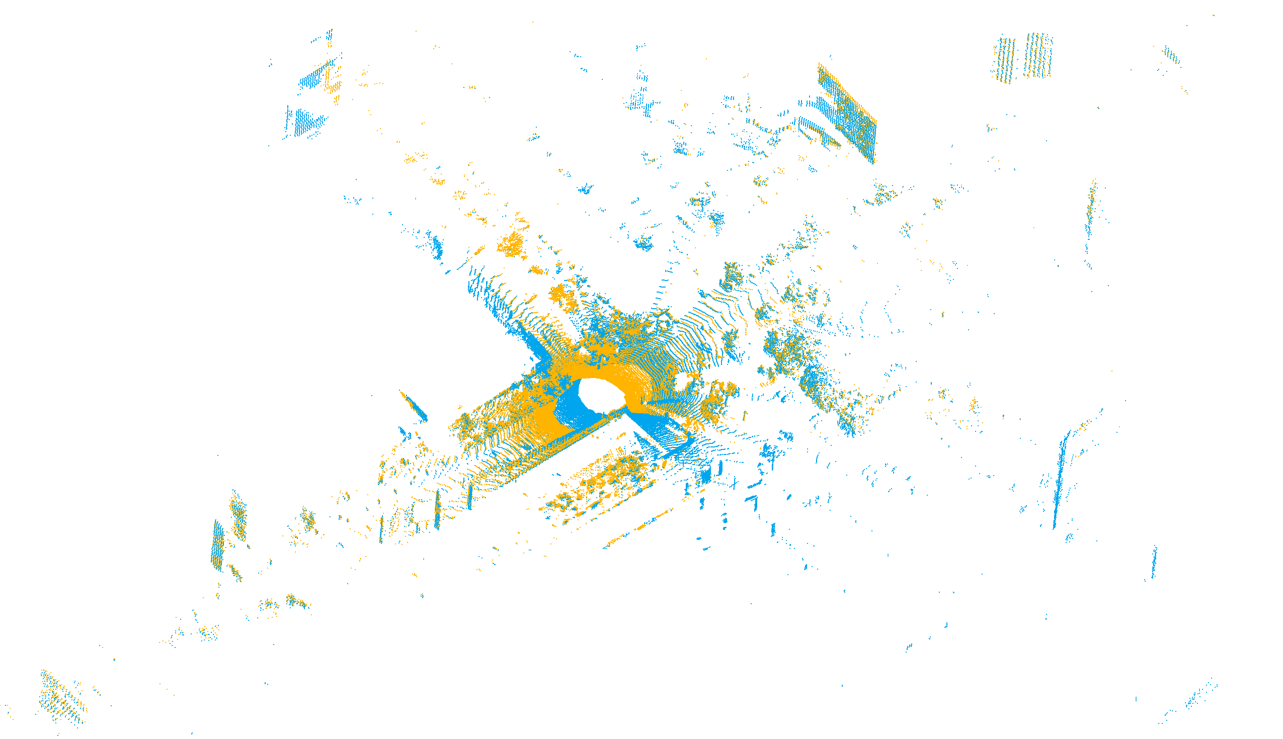
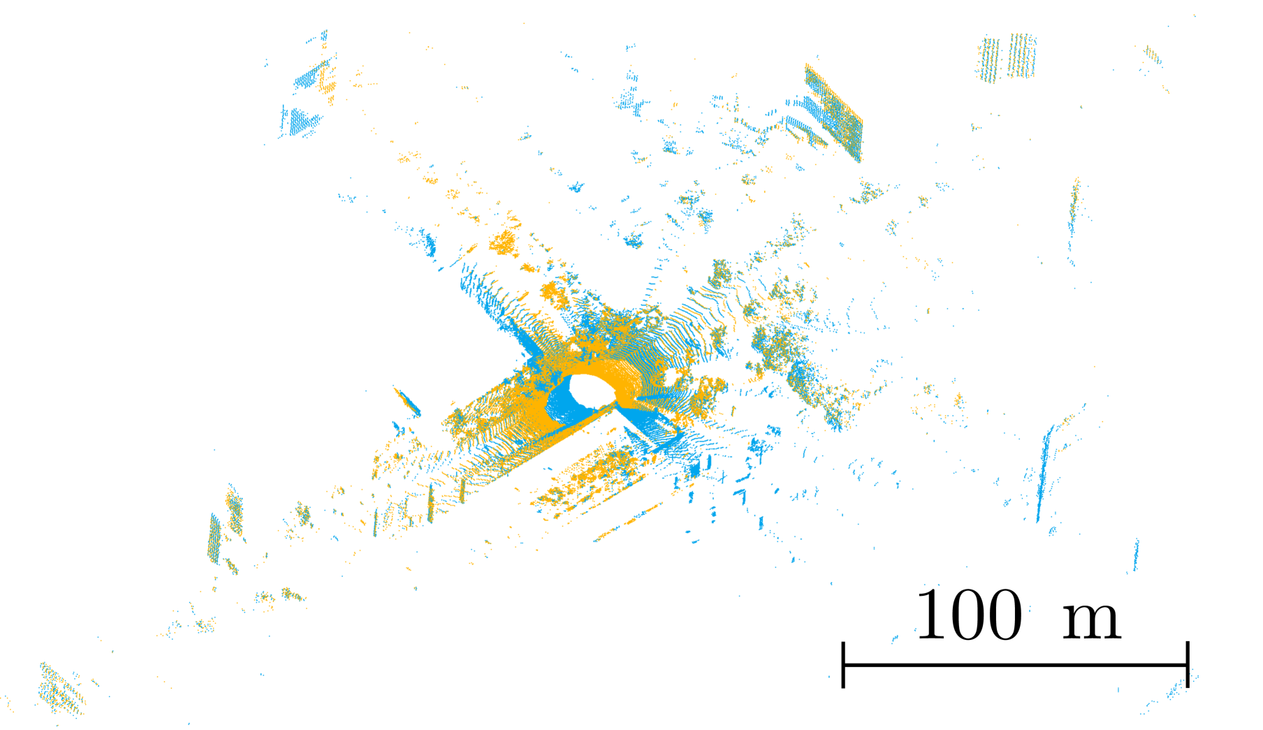
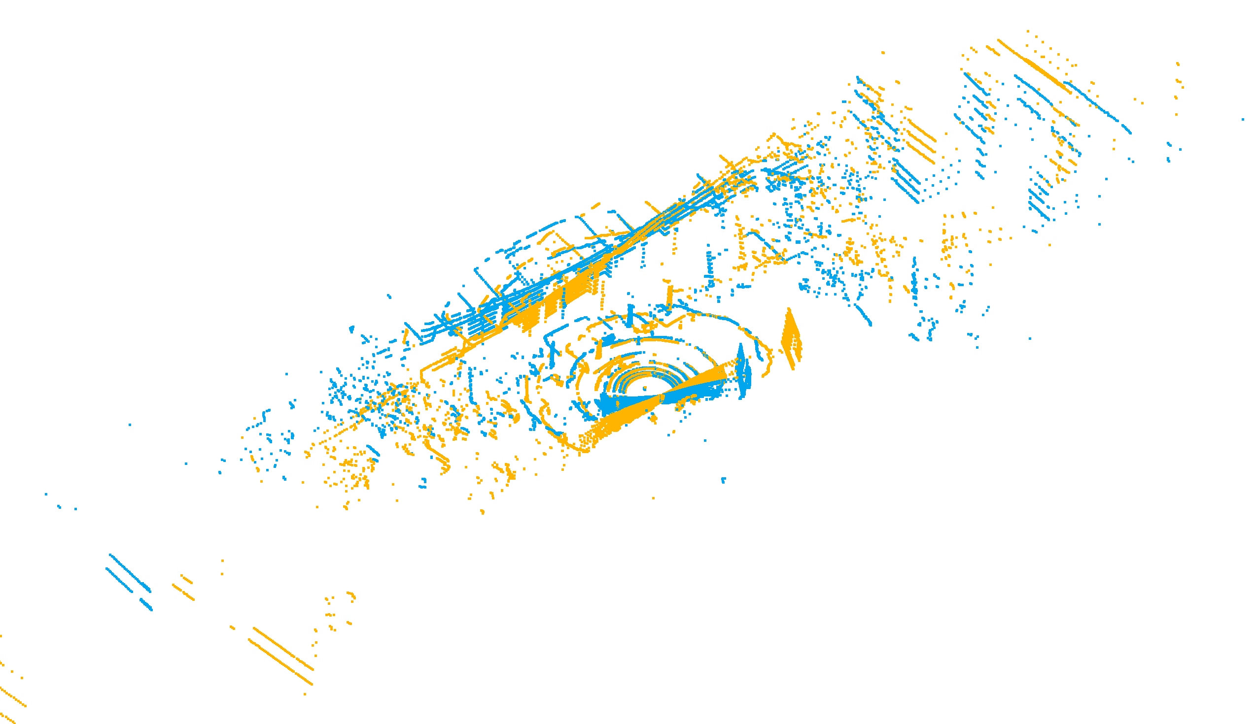
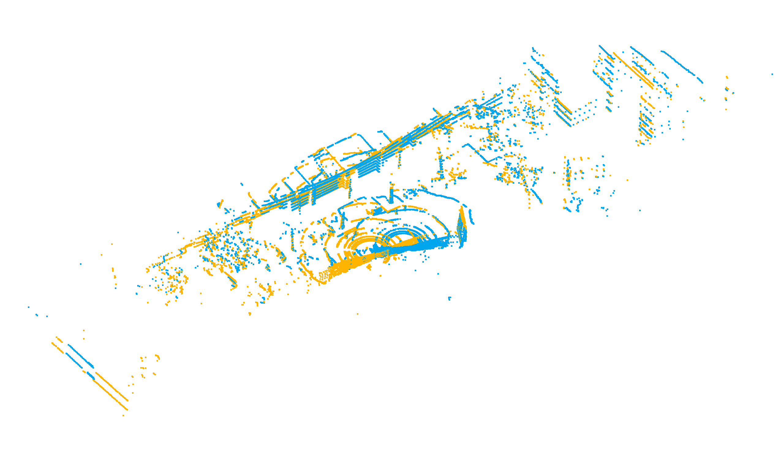
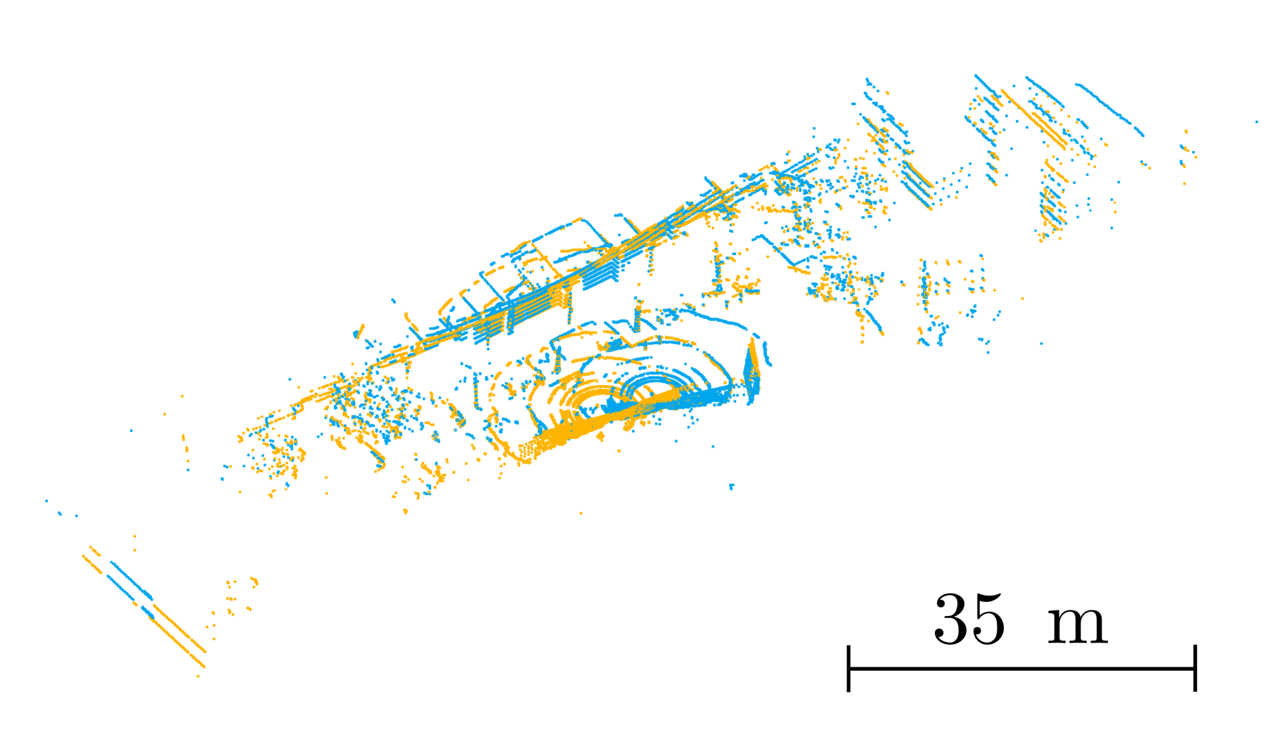
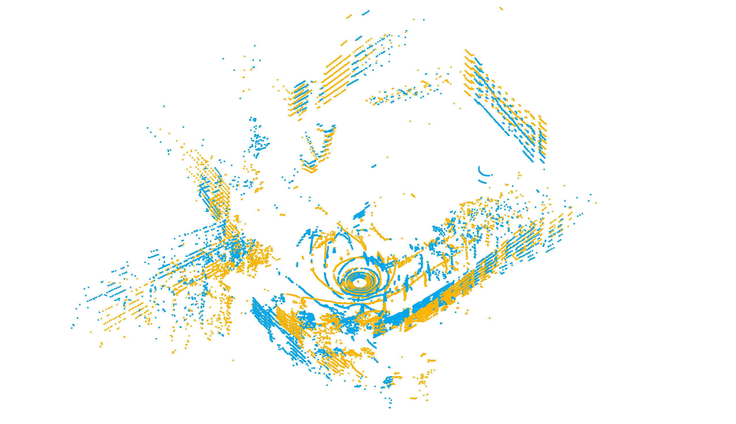
(a) Source and target

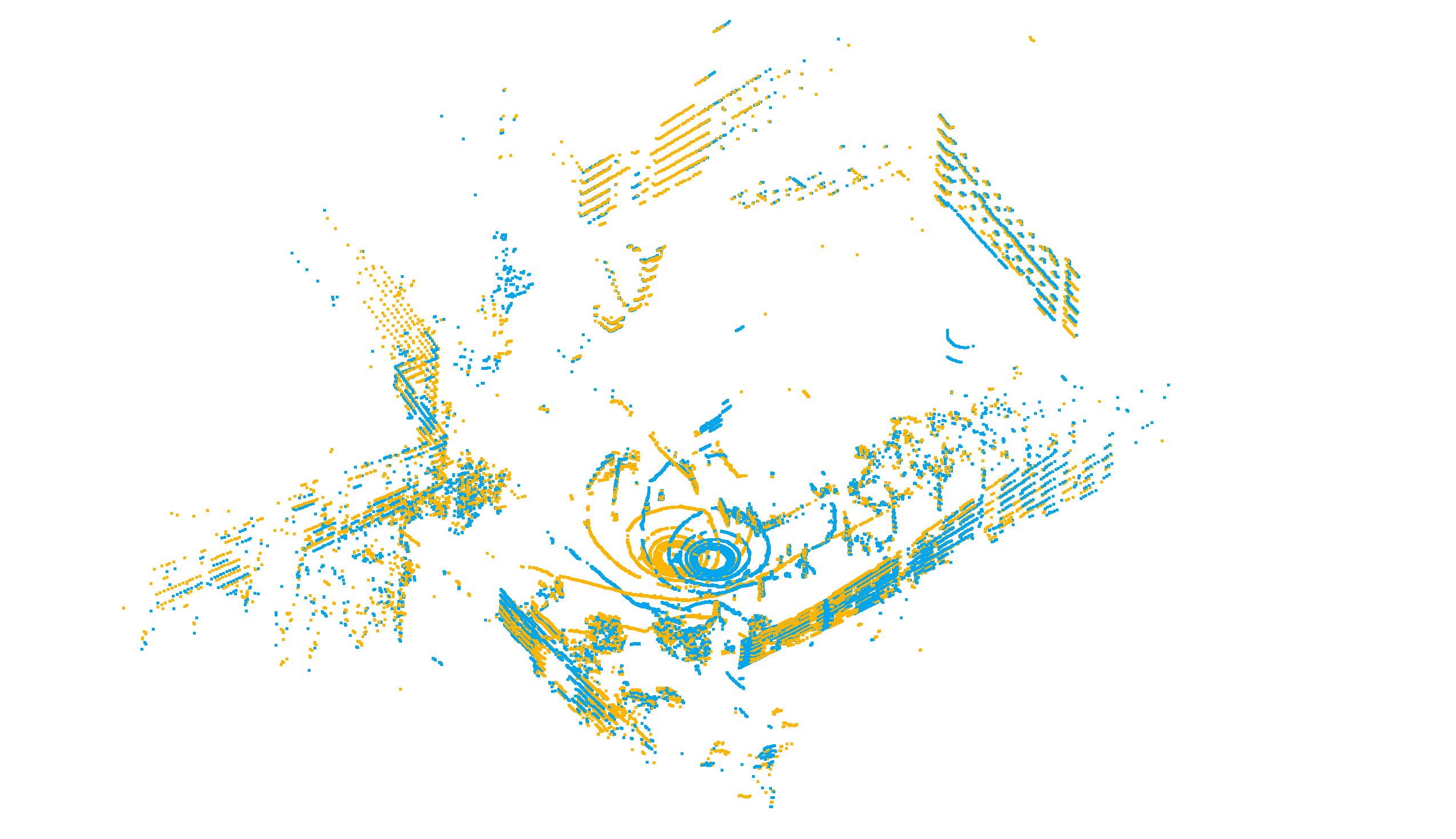
(b) BUFFER-X (Ours)

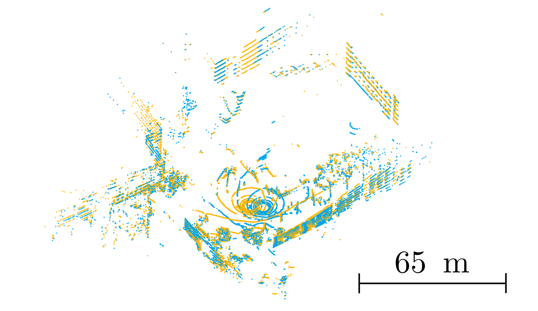
(c) Ground truth

Fig. A6: Qualitative results on outdoor point cloud registration: (T-B): Oxford, KAIST, and MIT sequences. (a) Input source (yellow) and target (blue) point clouds before registration. (b) Registration results obtained using our BUFFER-X. (c) Ground truth alignment. Visualization demonstrates that BUFFER-X achieves accurate alignment, closely matching the ground truth.

Therefore, these qualitative results further support the zero-shot registration capability of our BUFFER-X, regardless of the environment, sensor type, acquisition setup, or range.

	Env.	Indoor					Outdoor						Average rank
	Dataset	3DMatch	3DLoMatch	ScanNet++i	ScanNet++F	TIERS	KITTI	WOD	KAIST	MIT	ETH	Oxford
Conven- tional	FPFH [63] + FGR [94] +	62.53	15.42	77.68	92.31	80.60	98.74	100.00	89.80	74.78	91.87	99.00	8.55
	FPFH [63] + Quatro [43] +	8.22	1.74	9.88	97.27	86.57	99.10	100.00	91.46	79.57	51.05	91.03	10.82
	FPFH [63] + TEASER++ [77] +	52.00	13.25	66.15	97.22	73.13	98.92	100.00	89.20	71.30	93.69	99.34	8.82
Deep	FCGF [22]	8.04	0.17	19.96	23.07	77.82	98.92	95.38	88.34	82.17	6.59	75.08	14.82
	+	34.97	4.12	31.00	25.10	77.93	98.92	96.92	94.22	89.13	39.97	86.05	12.00
	+ +	34.97	4.12	33.37	25.10	77.93	98.92	99.23	94.22	90.43	39.97	90.03	11.27
	Predator [32]	N/A (Err)	N/A (Err)	N/A (Err)	N/A (Err)	69.43	99.82	100.00	N/A (OOM)	54.78	55.68	89.04	14.09
	+	16.47	0.00	9.40	3.72	69.77	99.82	100.00	71.3	76.52	56.67	89.04	12.00
	+ +	23.2	3.31	9.40	3.72	69.77	99.82	100.00	94.02	86.08	71.95	95.02	9.91
	GeoTransformer [59]	N/A (Err)	N/A (Err)	N/A (Err)	N/A (Err)	N/A (Err)	99.82	100.00	63.84	93.91	77.00	73.42	12.73
	+	5.94	0.30	15.91	34.18	20.57	99.82	100.00	63.84	93.91	77.56	73.42	10.90
	+ +	62.17	14.38	76.52	90.63	87.36	99.82	100.00	96.84	96.52	81.77	98.01	5.55
	BUFFER [5]	N/A (Err)	N/A (Err)	17.60	88.84	93.34	99.64	100.00	99.50	95.22	98.18	99.34	8.27
	+	91.19	64.51	93.15	97.81	93.57	99.64	100.00	99.55	97.39	99.86	99.34	3.27
	+ +	91.19	64.51	93.15	97.81	93.57	99.64	100.00	99.55	97.39	99.86	99.34	3.27
	PARENet [80]	N/A (Err)	N/A (Err)	N/A (Err)	N/A (Err)	N/A (Err)	99.82	97.69	57.51	75.22	68.30	66.11	15.82
	+	0.77	0.10	3.04	12.00	19.20	99.82	98.46	57.51	75.22	68.44	66.11	15.00
	+ +	22.09	4.98	29.99	42.91	52.99	99.82	100.00	89.50	87.39	72.65	94.02	9.18
	Ours with only $r_{m}$	91.96	63.59	92.38	99.45	94.37	99.82	100.00	99.55	99.13	100.00	99.67	1.82
	Ours	93.79	65.89	95.13	99.65	94.83	99.82	100.00	99.55	99.13	100.00	99.67	1.00

Table A3: Quantitative performance comparison on rate to evaluate generalization capability. All the models were trained only on KITTI [28] and RANSAC was used with the maximum iteration of 50K. The icons represent oracle tuning () to set proper voxel size and search radius to each dataset, and scale-up alignment () to normalize dataset scales to be similar to that of the KITTI data (e.g., the scale of 3DMatch, which typically uses a voxel size of 0.025, is adjusted to match the scale of KITTI, which typically uses a voxel size of 0.3, by multiplying by $\frac{0.3}{0.025}$). N/A (Err) indicates that the network cannot run due to an insufficient number of points remaining after voxelization with the voxel size typically used for outdoor settings, making keypoint extraction or descriptor generation infeasible. N/A (OOM) indicates an out-of-memory error caused by excessive memory usage.

F Quantitative results using KITTI

One may wonder how the model performs when trained on KITTI, so we also present the results of training on KITTI in Table A3. Interestingly, the success rates in 3DMatch and 3DLoMatch become slightly lower, while those in TIERS, KAIST, MIT, ETH improve when our BUFFER-X was trained on KITTI instead of 3DMatch. We speculate that because the model was trained on LiDAR data, it is better optimized for the distribution of LiDAR point clouds. Additionally, training on sparse point clouds results in exposure to relatively less diverse patch patterns, which may explain the performance drop when testing on 3DMatch.

Specifically, because the cloud points in 3DMatch are much denser than those in KITTI, randomly sampling $N_{\text{patch}}$ points from these clouds for each patch results in more varied local coordinate patterns. Thus, training in 3DMatch enables the model to learn more diverse local neighborhood patterns during training by randomly adjusting the size of $N_{\text{patch}}$. In contrast, in the case of KITTI, the points are relatively sparse because they are acquired using a LiDAR sensor. As a result, even when randomly sampling $N_{\text{patch}}$ points within the local neighborhoods, the diversity of local patterns remains relatively limited.

Moreover, our method demonstrated a higher rank compared to the state-of-the-art approaches. In particular, we observed that applying the voxel size used for outdoor training to indoor environments resulted in too few points remaining, leading to unexpected errors (referred to as “N/A (Err)” in Table A3). For example, when downsampling a $3\times 3\times 6$ m³ space with the 0.3 m voxel size, which is a typical size used for outdoor settings, only 2,000 points remain. In addition, we found that networks requiring large memory, such as Predator, encountered out-of-memory errors when processing denser point clouds (referred to as “N/A (OOM)” in Table A3). This means that an out-of-memory issue occurs when handling a 128-channel LiDAR point cloud without manual tuning of the parameters used for a 64-channel LiDAR point cloud.

Therefore, while training on KITTI led to some variations in overall performance, our approach remains more robust than other state-of-the-art methods in zero-shot registration.

References

- [1] Evangelos Alexiou, Xuemei Zhou, Irene Viola, and Pablo Cesar. PointPCA: Point cloud objective quality assessment using PCA-based descriptors. EURASIP Journal on Image and Video Processing, 2024(1):20, 2024.
- [2] Sheng Ao, Yulan Guo, Shangtai Gu, Jindong Tian, and Dong Li. SGHs for 3D local surface description. IET Computer Vision, 14(4):154–161, 2020.
- [3] Sheng Ao, Yulan Guo, Qingyong Hu, Bo Yang, Andrew Markham, and Zengping Chen. You only train once: Learning general and distinctive 3d local descriptors. IEEE Transactions on Pattern Analysis and Machine Intelligence, 45(3):3949–3967, 2022.
- [4] Sheng Ao, Yulan Guo, Jindong Tian, Yong Tian, and Dong Li. A repeatable and robust local reference frame for 3D surface matching. Pattern Recognition, 100:107186, 2020.
- [5] Sheng Ao, Qingyong Hu, Hanyun Wang, Kai Xu, and Yulan Guo. BUFFER: Balancing accuracy, efficiency, and generalizability in point cloud registration. In IEEE Conf. on Computer Vision and Pattern Recognition (CVPR), pages 1255–1264, 2023.
- [6] Sheng Ao, Qingyong Hu, Bo Yang, Andrew Markham, and Yulan Guo. SpinNet: Learning a general surface descriptor for 3D point cloud registration. In IEEE Conf. on Computer Vision and Pattern Recognition (CVPR), pages 11753–11762, 2021.
- [7] Koki Aoki, Kenji Koide, Shuji Oishi, Masashi Yokozuka, Atsuhiko Banno, and Junichi Meguro. 3D-BBS: Global localization for 3D point cloud scan matching using branch-and-bound algorithm. IEEE Intl. Conf. on Robotics and Automation (ICRA), pages 1796–1802, 2024.
- [8] Xuyang Bai, Zixin Luo, Lei Zhou, Hongbo Fu, Long Quan, and Chiew-Lan Tai. D3feat: Joint learning of dense detection and description of 3d local features. In IEEE Conf. on Computer Vision and Pattern Recognition (CVPR), 2020.
- [9] Jonathan T. Barron. A general and adaptive robust loss function, 2019.
- [10] Lukas Bernreiter, Lionel Ott, Juan Nieto, Roland Siegwart, and Cesar Cadena. PHASER: A robust and correspondence-free global point cloud registration. IEEE Robotics and Automation Letters, 6(2):855–862, 2021.
- [11] P. J. Besl and N. D. McKay. A method for registration of 3-D shapes. IEEE Trans. Pattern Anal. Machine Intell., 14(2), 1992.
- [12] Mark Brown, David Windridge, and Jean-Yves Guillemaut. A family of globally optimal branch-and-bound algorithms for 2D-3D correspondence-free registration. Pattern Recognition, 93:36–54, 2019.
- [13] Daniele Cattaneo, Matteo Vaghi, and Abhinav Valada. LCDNet: Deep loop closure detection and point cloud registration for LiDAR SLAM. IEEE Trans. Robotics, 38(4):2074–2093, 2022.
- [14] Y. Chang, Y. Tian, J.P. How, and L. Carlone. Kimera-Multi: a system for distributed multi-robot metric-semantic simultaneous localization and mapping. In IEEE Intl. Conf. on Robotics and Automation (ICRA), 2021. arXiv preprint: 2011.04087, (pdf).
- [15] Guangyan Chen, Meiling Wang, Yi Yang, Li Yuan, and Yufeng Yue. Fast and robust point cloud registration with tree-based transformer. In 2024 IEEE International Conference on Robotics and Automation (ICRA), pages 773–780, 2024.
- [16] Hong Chen, Pei Yan, Sihe Xiang, and Yihua Tan. Dynamic cues-assisted transformer for robust point cloud registration. In Proceedings of the IEEE/CVF Conference on Computer Vision and Pattern Recognition, pages 21698–21707, 2024.
- [17] Tianyi Chen, Bo Ji, Tianyu Ding, Biyi Fang, Guanyi Wang, Zhihui Zhu, Luming Liang, Yixin Shi, Sheng Yi, and Xiao Tu. Only train once: A one-shot neural network training and pruning framework. Advances in Neural Information Processing Systems, 34:19637–19651, 2021.
- [18] Xieyuanli Chen, Thomas Läbe, Andres Milioto, Timo Röhling, Jens Behley, and Cyrill Stachniss. OverlapNet: A siamese network for computing LiDAR scan similarity with applications to loop closing and localization. Autonomous Robots, 46(1):61–81, 2022.
- [19] Sunglok Choi, Taemin Kim, and Wonpil Yu. Performance evaluation of RANSAC family. J. of Computer Vision, 24(3):271–300, 1997.
- [20] Christopher Choy, Wei Dong, and Vladlen Koltun. Deep global registration. In IEEE Conf. on Computer Vision and Pattern Recognition (CVPR), 2020.
- [21] Christopher Choy, JunYoung Gwak, and Silvio Savarese. 4D Spatio-Temporal Convnets: Minkowski convolutional neural networks. In IEEE Conf. on Computer Vision and Pattern Recognition (CVPR), pages 3075–3084, 2019.
- [22] Christopher Choy, Jaesik Park, and Vladlen Koltun. Fully convolutional geometric features. In Intl. Conf. on Computer Vision (ICCV), pages 8958–8966, 2019.
- [23] Ondřej Chum, Jiří Matas, and Josef Kittler. Locally optimized RANSAC. In Joint Pattern Recognition Symposium, pages 236–243, 2003.
- [24] Zhen Dong, Bisheng Yang, Yuan Liu, Fuxun Liang, Bijun Li, and Yufu Zang. A novel binary shape context for 3D local surface description. ISPRS Journal of Photogrammetry and Remote Sensing, 130:431–452, 2017.
- [25] Alexey Dosovitskiy and Josip Djolonga. You only train once: Loss-conditional training of deep networks. In International conference on learning representations, 2019.
- [26] Kaveh Fathian and Tyler Summers. CLIPPER+: A Fast Maximal Clique Algorithm for Robust Global Registration. IEEE Robotics and Automation Letters, 2024.
- [27] M. Fischler and R. Bolles. Random sample consensus: a paradigm for model fitting with application to image analysis and automated cartography. Commun. ACM, 24:381–395, 1981.
- [28] Andreas Geiger, Philip Lenz, Christoph Stiller, and Raquel Urtasun. Vision meets robotics: The KITTI dataset. Intl. J. of Robotics Research, 32(11):1231–1237, 2013.
- [29] Signe Schilling Hansen, Verner Brandbyge Ernstsen, Mikkel Skovgaard Andersen, Zyad Al-Hamdani, Ramona Baran, Manfred Niederwieser, Frank Steinbacher, and Aart Kroon. Classification of boulders in coastal environments using random forest machine learning on topo-bathymetric LiDAR data. Remote Sensing, 13(20):4101, 2021.
- [30] Chris Harris, Mike Stephens, et al. A combined corner and edge detector. In Alvey vision conference, pages 10–5244, 1988.
- [31] R.I. Hartley and F. Kahl. Global optimization through rotation space search. Intl. J. of Computer Vision, 82(1):64–79, 2009.
- [32] Shengyu Huang, Zan Gojcic, Mikhail Usvyatsov, Andreas Wieser, and Konrad Schindler. PREDATOR: Registration of 3D Point Clouds with Low Overlap. In IEEE Conf. on Computer Vision and Pattern Recognition (CVPR), pages 4265–4274, Jun. 2021.
- [33] Tianyu Huang, Liangzu Peng, Rene Vidal, and Yun-Hui Liu. Scalable 3D Registration via Truncated Entry-wise Absolute Residuals. In Proceedings of the IEEE/CVF Conference on Computer Vision and Pattern Recognition (CVPR), pages 27477–27487, June 2024.
- [34] Minwoo Jung, Wooseong Yang, Dongjae Lee, Hyeonjae Gil, Giseop Kim, and Ayoung Kim. HeLiPR: Heterogeneous LiDAR dataset for inter-LiDAR place recognition under spatial and temporal variations. The International Journal of Robotics Research, 2023.
- [35] Diederik P Kingma. Adam: A method for stochastic optimization. arXiv preprint arXiv:1412.6980, 2014.
- [36] Kenji Koide, Masashi Yokozuka, Shuji Oishi, and Atsuhiko Banno. Voxelized GICP for fast and accurate 3D point cloud registration. In IEEE Intl. Conf. on Robotics and Automation (ICRA), pages 11054–11059, 2021.
- [37] Kanghee Lee, Junha Lee, and Jaesik Park. Learning to register unbalanced point pairs. arXiv preprint arXiv:2207.04221, 2022.
- [38] Huan Lei, Guang Jiang, and Long Quan. Fast descriptors and correspondence propagation for robust global point cloud registration. IEEE Trans. Image Processing, 26(8):3614–3623, 2017.
- [39] Hyungtae Lim, Seoyeon Jang, Benedikt Mersch, Jens Behley, Hyun Myung, and Cyrill Stachniss. Helimos: A dataset for moving object segmentation in 3d point clouds from heterogeneous lidar sensors. In IEEE/RSJ International Conference on Intelligent Robots and Systems (IROS), pages 14087–14094, 2024.
- [40] Hyungtae Lim, Beomsoo Kim, Daebeom Kim, Eungchang Mason Lee, and Hyun Myung. Quatro++: Robust global registration exploiting ground segmentation for loop closing in LiDAR SLAM. Intl. J. of Robotics Research, pages 685–715, 2024.
- [41] Hyungtae Lim, Daebeom Kim, Gunhee Shin, Jingnan Shi, Ignacio Vizzo, Hyun Myung, Jaesik Park, and Luca Carlone. KISS-Matcher: Fast and Robust Point Cloud Registration Revisited. IEEE Intl. Conf. on Robotics and Automation (ICRA), 2025. Accepted. To appear.
- [42] Hyungtae Lim, Minho Oh, and Hyun Myung. Patchwork: Concentric zone-based region-wise ground segmentation with ground likelihood estimation using a 3D LiDAR sensor. IEEE Robotics and Automation Letters, 6(4):6458–6465, 2021.
- [43] Hyungtae Lim, Suyong Yeon, Soohyun Ryu, Yonghan Lee, Youngji Kim, Jaeseong Yun, Euigon Jung, Donghwan Lee, and Hyun Myung. A single correspondence is enough: Robust global registration to avoid degeneracy in urban environments. In IEEE Intl. Conf. on Robotics and Automation (ICRA), pages 8010–8017, 2022.
- [44] Quan Liu, Hongzi Zhu, Zhenxi Wang, Yunsong Zhou, Shan Chang, and Minyi Guo. Extend your own correspondences: Unsupervised distant point cloud registration by progressive distance extension. In Proceedings of the IEEE/CVF Conference on Computer Vision and Pattern Recognition, pages 20816–20826, 2024.
- [45] Shaocong Liu, Tao Wang, Yan Zhang, Ruqin Zhou, Li Li, Chenguang Dai, Yongsheng Zhang, Longguang Wang, and Hanyun Wang. Deep semantic graph matching for large-scale outdoor point cloud registration. IEEE Transactions on Geoscience and Remote Sensing, 2024.
- [46] Xin Liu, Rong Qin, Junchi Yan, and Jufeng Yang. Ncmnet: Neighbor consistency mining network for two-view correspondence pruning. IEEE Transactions on Pattern Analysis and Machine Intelligence, 2024.
- [47] D.G. Lowe. Distinctive image features from scale-invariant keypoints. Intl. J. of Computer Vision, 60(2):91–110, 2004.
- [48] Johan Ernest Mebius. Derivation of the Euler-Rodrigues formula for three-dimensional rotations from the general formula for four-dimensional rotations. arXiv preprint math/0701759, 2007.
- [49] Juncheng Mu, Lin Bie, Shaoyi Du, and Yue Gao. ColorPCR: Color point cloud registration with multi-stage geometric-color fusion. In Proceedings of the IEEE/CVF Conference on Computer Vision and Pattern Recognition, pages 21061–21070, 2024.
- [50] Carl Olsson, Fredrik Kahl, and Magnus Oskarsson. Branch-and-bound methods for euclidean registration problems. IEEE Trans. Pattern Anal. Machine Intell., 31(5):783–794, 2009.
- [51] Jin Pan, Zhe Min, Ang Zhang, Han Ma, and Max Q-H Meng. Multi-view global 2D-3D registration based on branch and bound algorithm. In Proc. IEEE Int. Conf. Robot. Biomim., pages 3082–3087, 2019.
- [52] Chavdar Papazov, Sami Haddadin, Sven Parusel, Kai Krieger, and Darius Burschka. Rigid 3D geometry matching for grasping of known objects in cluttered scenes. Intl. J. of Robotics Research, 31(4):538–553, 2012.
- [53] Fabio Poiesi and Davide Boscaini. Distinctive 3D local deep descriptors. In Intl. Conf. on Pattern Recognition (ICPR), pages 5720–5727, 2021.
- [54] Fabio Poiesi and Davide Boscaini. Learning general and distinctive 3D local deep descriptors for point cloud registration. IEEE Trans. Pattern Anal. Machine Intell., 45(3):3979–3985, 2022.
- [55] F. Pomerleau, F. Colas, R. Siegwart, and S. Magnenat. Comparing ICP variants on real-world data sets. Autonomous Robots, 34(3):133–148, 2013.
- [56] François Pomerleau, Ming Liu, Francis Colas, and Roland Siegwart. Challenging data sets for point cloud registration algorithms. The International Journal of Robotics Research, 31(14):1705–1711, 2012.
- [57] F. Pomerleau, M. Liu, F. Colas, and R. Siegwart. Challenging data sets for point cloud registration algorithms. Intl. J. of Robotics Research, 31(14):1705–1711, 2012.
- [58] Charles R Qi, Hao Su, Kaichun Mo, and Leonidas J Guibas. Pointnet: Deep learning on point sets for 3D classification and segmentation. In IEEE Conf. on Computer Vision and Pattern Recognition (CVPR), pages 652–660, 2017.
- [59] Zheng Qin, Hao Yu, Changjian Wang, Yulan Guo, Yuxing Peng, Slobodan Ilic, Dewen Hu, and Kai Xu. GeoTransformer: Fast and robust point cloud registration with geometric transformer. IEEE Transactions on Pattern Analysis and Machine Intelligence, 45(8):9806–9821, 2023.
- [60] Li Qingqing, Yu Xianjia, Jorge Pena Queralta, and Tomi Westerlund. Multi-modal LiDAR dataset for benchmarking general-purpose localization and mapping algorithms. In IEEE/RSJ Intl. Conf. on Intelligent Robots and Systems (IROS), pages 3837–3844, 2022.
- [61] Milad Ramezani, Yiduo Wang, Marco Camurri, David Wisth, Matias Mattamala, and Maurice Fallon. The newer college dataset: Handheld lidar, inertial and vision with ground truth. In 2020 IEEE/RSJ International Conference on Intelligent Robots and Systems (IROS), pages 4353–4360. IEEE, 2020.
- [62] Mohammad Rouhani and Angel D Sappa. Correspondence free registration through a point-to-model distance minimization. In Intl. Conf. on Computer Vision (ICCV), pages 2150–2157, 2011.
- [63] R.B. Rusu, N. Blodow, and M. Beetz. Fast point feature histograms (fpfh) for 3d registration. In IEEE Intl. Conf. on Robotics and Automation (ICRA), pages 3212–3217. Citeseer, 2009.
- [64] Kwonyoung Ryu, Soonmin Hwang, and Jaesik Park. Instant domain augmentation for lidar semantic segmentation. In Proceedings of the IEEE/CVF Conference on Computer Vision and Pattern Recognition, pages 9350–9360, 2023.
- [65] Ruwen Schnabel, Roland Wahl, and Reinhard Klein. Efficient RANSAC for point-cloud shape detection. In Computer Graphics Forum, pages 214–226, 2007.
- [66] Aleksandr Segal, Dirk Haehnel, and Sebastian Thrun. Generalized ICP. In Robotics: Science and Systems (RSS), Jun. 2009.
- [67] Pengcheng Shi, Shaocheng Yan, Yilin Xiao, Xinyi Liu, Yongjun Zhang, and Jiayuan Li. RANSAC back to SOTA: A two-stage consensus filtering for real-time 3D registration. IEEE Robotics and Automation Letters, 2024.
- [68] Lei Sun and Lu Deng. TriVoC: Efficient voting-based consensus maximization for robust point cloud registration with extreme outlier ratios. IEEE Robotics and Automation Letters, 7(2):4654–4661, 2022.
- [69] Pei Sun, Henrik Kretzschmar, Xerxes Dotiwalla, Aurelien Chouard, Vijaysai Patnaik, Paul Tsui, James Guo, Yin Zhou, Yuning Chai, Benjamin Caine, et al. Scalability in perception for autonomous driving: Waymo open dataset. In Proceedings of the IEEE/CVF Conference on Computer Vision and Pattern Recognition, pages 2446–2454, 2020.
- [70] Hugues Thomas, Charles R Qi, Jean-Emmanuel Deschaud, Beatriz Marcotegui, François Goulette, and Leonidas J Guibas. Kpconv: Flexible and deformable convolution for point clouds. In Proceedings of the IEEE/CVF international conference on computer vision, pages 6411–6420, 2019.
- [71] Y. Tian, Y. Chang, L. Quang, A. Schang, C. Nieto-Granda, J.P. How, and L. Carlone. Resilient and distributed multi-robot visual SLAM: Datasets, experiments, and lessons learned. In IEEE/RSJ Intl. Conf. on Intelligent Robots and Systems (IROS), 2023. (pdf),(video),(code),(web).
- [72] Ignacio Vizzo, Tiziano Guadagnino, Benedikt Mersch, Louis Wiesmann, Jens Behley, and Cyrill Stachniss. KISS-ICP: In defense of point-to-point ICP – Simple, accurate, and robust registration if done the right way. IEEE Robotics and Automation Letters, pages 1029–1036, 2023.
- [73] Xiaoyang Wu, Li Jiang, Peng-Shuai Wang, Zhijian Liu, Xihui Liu, Yu Qiao, Wanli Ouyang, Tong He, and Hengshuang Zhao. Point Transformer V3: Simpler Faster Stronger. In Proceedings of the IEEE/CVF Conference on Computer Vision and Pattern Recognition, pages 4840–4851, 2024.
- [74] Xiaoyang Wu, Yixing Lao, Li Jiang, Xihui Liu, and Hengshuang Zhao. Point transformer v2: Grouped vector attention and partition-based pooling. Advances in Neural Information Processing Systems, 35:33330–33342, 2022.
- [75] H. Yang, P. Antonante, V. Tzoumas, and L. Carlone. Graduated non-convexity for robust spatial perception: From non-minimal solvers to global outlier rejection. IEEE Robotics and Automation Letters (RA-L), 5(2):1127–1134, 2020. arXiv preprint:1909.08605 (with supplemental material), (pdf).
- [76] H. Yang and L. Carlone. A polynomial-time solution for robust registration with extreme outlier rates. In Robotics: Science and Systems (RSS), 2019. (pdf), (video), (media), (media), (media).
- [77] H. Yang, J. Shi, and L. Carlone. TEASER: Fast and Certifiable Point Cloud Registration. IEEE Trans. Robotics, 37(2):314–333, 2020. extended arXiv version 2001.07715 (pdf).
- [78] J. Yang, H. Li, D. Campbell, and Y. Jia. Go-ICP: A globally optimal solution to 3D ICP point-set registration. IEEE Trans. Pattern Anal. Machine Intell., 38(11):2241–2254, Nov. 2016.
- [79] Jiaqi Yang, Xiyu Zhang, Peng Wang, Yulan Guo, Kun Sun, Qiao Wu, Shikun Zhang, and Yanning Zhang. MAC: Maximal Cliques for 3D Registration. IEEE Transactions on Pattern Analysis and Machine Intelligence, 2024.
- [80] Runzhao Yao, Shaoyi Du, Wenting Cui, Canhui Tang, and Chengwu Yang. Pare-net: Position-aware rotation-equivariant networks for robust point cloud registration. In European Conference on Computer Vision, pages 287–303. Springer, 2024.
- [81] Chandan Yeshwanth, Yueh-Cheng Liu, Matthias Nießner, and Angela Dai. Scannet++: A high-fidelity dataset of 3d indoor scenes. In Proceedings of the IEEE/CVF International Conference on Computer Vision, pages 12–22, 2023.
- [82] Z.J. Yew and G.H. Lee. 3dfeat-net: Weakly supervised local 3d features for point cloud registration. In European Conf. on Computer Vision (ECCV), 2018.
- [83] Huan Yin, Xuecheng Xu, Sha Lu, Xieyuanli Chen, Rong Xiong, Shaojie Shen, Cyrill Stachniss, and Yue Wang. A survey on global lidar localization: Challenges, advances and open problems. Intl. J. of Computer Vision, pages 1–33, 2024.
- [84] Pengyu Yin, Shenghai Yuan, Haozhi Cao, Xingyu Ji, Shuyang Zhang, and Lihua Xie. Segregator: Global point cloud registration with semantic and geometric cues. In IEEE Intl. Conf. on Robotics and Automation (ICRA), pages 2848–2854, 2023.
- [85] Hao Yu, Fu Li, Mahdi Saleh, Benjamin Busam, and Slobodan Ilic. CofiNet: reliable coarse-to-fine correspondences for robust pointcloud registration. Advances in Neural Information Processing Systems, 34:23872–23884, 2021.
- [86] Zhiyuan Yu, Zheng Qin, Lintao Zheng, and Kai Xu. Learning instance-aware correspondences for robust multi-instance point cloud registration in cluttered scenes. In Proceedings of the IEEE/CVF Conference on Computer Vision and Pattern Recognition (CVPR), pages 19605–19614, June 2024.
- [87] Yongzhe Yuan, Yue Wu, Xiaolong Fan, Maoguo Gong, Qiguang Miao, and Wenping Ma. Inlier confidence calibration for point cloud registration. In Proceedings of the IEEE/CVF Conference on Computer Vision and Pattern Recognition, pages 5312–5321, 2024.
- [88] Andy Zeng, Shuran Song, Matthias Nießner, Matthew Fisher, Jianxiong Xiao, and T Funkhouser. 3DMatch: Learning the matching of local 3d geometry in range scans. In IEEE Conf. on Computer Vision and Pattern Recognition (CVPR), page 4, 2017.
- [89] Xinyue Zhang, Liangzu Peng, Wanting Xu, and Laurent Kneip. Accelerating globally optimal consensus maximization in geometric vision. IEEE Transactions on Pattern Analysis and Machine Intelligence, 46(6):4280–4297, 2024.
- [90] Xiyu Zhang, Jiaqi Yang, Shikun Zhang, and Yanning Zhang. 3D registration with maximal cliques. In Proceedings of the IEEE/CVF Conference on Computer Vision and Pattern Recognition, pages 17745–17754, 2023.
- [91] Yifei Zhang, Hao Zhao, Hongyang Li, and Siheng Chen. FastMAC: Stochastic Spectral Sampling of Correspondence Graph. In Proceedings of the IEEE/CVF Conference on Computer Vision and Pattern Recognition, pages 17857–17867, 2024.
- [92] Zhengyou Zhang. Parameter estimation techniques: A tutorial with application to conic fitting. Image and vision Computing, 15(1):59–76, 1997.
- [93] Mingyang Zhao, Jingen Jiang, Lei Ma, Shiqing Xin, Gaofeng Meng, and Dong-Ming Yan. Correspondence-free non-rigid point set registration using unsupervised clustering analysis. In Proceedings of the IEEE/CVF Conference on Computer Vision and Pattern Recognition, pages 21199–21208, 2024.
- [94] Qian-Yi Zhou, Jaesik Park, and Vladlen Koltun. Fast global registration. In Proceedings of the European Conference on Computer Vision (ECCV), pages 766–782, 2016.
- [95] Xinge Zhu, Hui Zhou, Tai Wang, Fangzhou Hong, Yuexin Ma, Wei Li, Hongsheng Li, and Dahua Lin. Cylindrical and asymmetrical 3d convolution networks for lidar segmentation. In Proceedings of the IEEE/CVF conference on computer vision and pattern recognition, pages 9939–9948, 2021.