CAD-VAE: Leveraging Correlation-Aware Latents for Comprehensive Fair Disentanglement

Abstract

While deep generative models have significantly advanced representation learning, they may inherit or amplify biases and fairness issues by encoding sensitive attributes alongside predictive features. Enforcing strict independence in disentanglement is often unrealistic when target and sensitive factors are naturally correlated. To address this challenge, we propose CAD-VAE (Correlation-Aware Disentangled VAE), which introduces a correlated latent code to capture the shared information between target and sensitive attributes. Given this correlated latent, our method effectively separates overlapping factors without extra domain knowledge by directly minimizing the conditional mutual information between target and sensitive codes. A relevance-driven optimization strategy refines the correlated code by efficiently capturing essential correlated features and eliminating redundancy. Extensive experiments on benchmark datasets demonstrate that CAD-VAE produces fairer representations, realistic counterfactuals, and improved fairness-aware image editing. Code

1 Introduction

Deep generative models have achieved remarkable success in capturing complex data distributions for applications ranging from image synthesis [1] to video generation [34]. In particular, variational autoencoders (VAEs)[13, 21, 31, 33] have provided a principled approach to representation learning, where data are encoded into compact latent variables that effectively capture meaningful factors of variation. However, while these latent representations have enabled impressive performance in numerous tasks, concerns about fairness have emerged, as models can inadvertently learn and amplify biases present in training data[15].

Such fairness issues arise when the target label and sensitive label become entangled due to societal or dataset biases [24, 26]. To address these problems, existing methods commonly fall into two categories. Invariant learning techniques aim to remove sensitive attributes from the learned representation, often via adversarial training or additional regularization [24, 40]. By contrast, disentanglement approaches encourage the model to partition its latent space into separate codes for target and sensitive information, seeking statistical independence among them [6, 28]. Although these solutions have made progress, they typically assume minimal correlation between target and sensitive factors or enforce strict separation via mutual information penalties [3]. However, multiple works [15, 36] have demonstrated that achieving fully fair disentanglement is fundamentally impossible under realistic conditions. First, many datasets contain unwanted correlations between the target label and sensitive attributes due to societal bias, making it infeasible to preserve all predictive cues while completely discarding sensitive information [8]. Second, certain features inherently influence both target and sensitive attributes, so perfectly partitioning features into disjoint latent spaces is unachievable without compromising prediction accuracy [22]. In these circumstances, any attempt at full disentanglement faces an inevitable trade-off between fairness and utility.

A natural way to handle this correlation is to explicitly model how target and sensitive attributes overlap. For instance, some methods rely on causal graphs to separate task-relevant features and capture their relationships with sensitive variables [20, 41, 51, 14]. However, constructing such graphs requires extensive domain knowledge, which is often challenging to acquire in real-world scenarios.

Motivated by the limitations of existing methods, we introduce an additional latent code specifically designed to capture the shared information between target and sensitive attributes. Our approach directly minimizes the conditional mutual information between target and sensitive property predictions, conditioned on this correlated latent code. This design guarantees that the target and sensitive latent codes remain independent once the overlapping factors are absorbed. Moreover, an explicit relevance learning strategy ensures that the correlated latent code captures only the essential shared information without extra domain knowledge. In summary, our contributions are as follows:

1. We propose a novel correlation-aware representation learning framework that directly minimizes the conditional mutual information between target and sensitive property, conditioned on the correlated latent code, effectively addressing the conflict between predictive objectives and disentanglement.

2. We introduce an explicit relevance-driven optimization strategy that precisely regulates the correlated latent code, ensuring it captures only the essential shared information without extra domain knowledge.

3. We validate our approach through comprehensive experiments on multiple benchmark datasets, demonstrating its superiority in achieving correlation-aware disentanglement, enhancing fair prediction performance, and improving both counterfactual generation and fairness-aware image editing, as well as its broad applicability in the context of Vision-Language Models (VLM).

2 Related Work

2.1 Fair Disentanglement Learning

Instead of directly learning sensitive-information-free representations [28, 30, 46], Fair Disentanglement Learning focuses on disentangling these representations into two sets of latent variables, each dedicated to capturing target or sensitive information separately [43]. One of the pioneering works, $\beta$-VAE [13], introduced a framework for semantic feature disentanglement by enforcing a stronger prior constraint on the variational distribution. Extending this idea, FactorVAE [19] proposed minimizing the total correlation (TC) among latent variables to achieve a more refined decomposition of latent space. Specifically, FactorVAE introduces a discriminator-based approach to approximate the TC loss as:

$$L_{TC}=KL(q(z)||\prod_{j}q(z_{j}))\approx\mathbb{E}{q_{\phi}(z)}\left[\log\frac{D(z)}{1-D(z)}\right],$$ (1)

where the discriminator $D$ aims to distinguish whether the latent code $z$ is sampled from the aggregate posterior or from a combination of in-batch permutations of marginal distributions across each latent dimension $j$. Meanwhile, the encoder is trained to fool the discriminator, promoting independence among latent dimensions. Further advancements on FactorVAE, FairFactorVAE [28] incorporate strategies to obfuscate sensitive information within the latent space, enhancing privacy preservation.

Another notable approach, FFVAE [6], extends the use of total correlation [3] specifically to disentangle the sensitive code with adaptability to the dimension of sensitive information. GVAE [7] employs adversarial training to minimize the leakage of unwanted information in each latent code, offering an alternative method to enforce independence between target and sensitive representations. Meanwhile, ODVAE [42] introduces orthogonal priors for target and sensitive codes, ensuring that these codes maintain minimal overlap. FairDisCo [27] approaches the independence challenge through distance covariance minimization, offering a non-adversarial alternative to traditional methods.

2.2 Correlation-Aware Learning

While disentanglement methods advance different information separations, achieving perfectly independent latent codes remains challenging. The need to recover both sensitive and target information often conflicts with maintaining complete independence, as these types of information are frequently correlated in practice [32, 15]. For instance, in facial attribute recognition on the CelebA dataset [29], ’mustache’ (sensitive relevant) correlates with both gender (sensitive) and attractiveness (target), highlighting the inherent dependency between sensitive and target codes.

To address the challenge of correlated information, Correlation-Aware Learning [20, 41, 51, 14] employs a causal graph approach to separate latent variables based on their correlation with sensitive information. However, constructing such graphs requires domain knowledge and may not always be feasible. Additionally, not accounting for causal relationships between variables can hinder the independence of learned latent codes, leading to practical and computational challenges [15].

To address the inherent correlation between target and sensitive information while reducing dependence on domain knowledge, FADES [15] proposes a novel approach that minimizes conditional mutual information by grouping samples based on different attributes to learn shared information in the sensitive relevant code. Although innovative, this indirect method may not effectively eliminate unwanted information leakage and lacks explicit guidance to ensure the sensitive relevant code captures an appropriate and balanced amount of information. These limitations motivate our approach, which directly minimizes conditional mutual information to achieve complete disentanglement and provides explicit constraints to ensure accurate relevance capture.

2.3 Counterfactual Fairness

Counterfactual fairness (CF) ensures fairness by evaluating whether predictions remain consistent when sensitive attributes are altered while keeping other features unchanged, aiming to mitigate bias through comparisons between factual and counterfactual outcomes [23]. The causal inference technique is widely adopted to generate these counterfactual instances [50, 16, 51, 4, 45], enabling a comparative analysis between actual and hypothetical scenarios.

Graph-based models with predefined intervention and individual variables [20, 25] use causal effect analysis to capture feature interactions for realistic counterfactuals. However, their effectiveness relies on precise domain knowledge; without it, generated counterfactuals may become unrealistic or nonsensical, such as depicting a girl with a mustache.

While CF demonstrates strong theoretical foundations, its dependence on precise domain knowledge complicates model design and may limit practical utility. To address this, our approach introduces a correlated latent code with an explicit relevance learning strategy, allowing the model to learn attribute relationships autonomously and enhance counterfactual fairness without external knowledge.

3 Method

3.1 CAD-VAE

Let $\mathcal{D}=\{(x_{i},y_{i},s_{i})\}_{i=1}^{N}$ denote a dataset consisting of triplets, where $x_{i}$ denotes an input sample (e.g., an image), $y_{i}$ is the label of $x_{i}$ corresponding to target property $Y$, and $s_{i}$ is the label corresponding to the sensitive property $S$. The value range of $Y$ and $S$ is $\mathcal{Y}$ and $\mathcal{S}$, respectively, i.e., $y\in\mathcal{Y}$ and $s\in\mathcal{S}$. The goal is to learn a latent representation that factorizes the information pertinent to $Y$, the information pertinent to $S$, the shared information between $Y$ and $S$, and the background or irrelevant factors. We introduce the following latent representations to capture different information:

• $z_{X}$: captures task-irrelevant information.

• $z_{Y}$: encodes the information strongly correlated with $Y$.

• $z_{S}$: encodes the information strongly correlated with $S$.

• $z_{R}$: represents the shared information between $Y$ and $S$.

Hence, for a single observation, the corresponding latent variable set is $z:=(z_{X},z_{Y},z_{S},z_{R})$. We first present the problem definition, model components, and architecture in Section 3.1, which serve as crucial foundations for the subsequent sections. To achieve correlation-aware disentanglement learning, we propose directly minimizing the conditional mutual information between $z_{Y}$ and $z_{S}$ with respect to their corresponding opposite attributes $S$ and $Y$, conditioned on $z_{R}$. This approach is complemented by an explicit relevance learning strategy that constrains $z_{R}$ to effectively capture shared information between $Y$ and $S$ while avoiding redundant information. Detailed explanations of these strategies are provided in Section 3.3 and Section 3.4, respectively.

To learn such latent code, we employ a Variational Autoencoder (VAE) [13] with an encoder $q_{\phi}(z\mid x)$ and a decoder $p_{\theta}(x\mid z)$ as our backbone. The prior distribution over the latent variables $p_{\theta}(z)$ is typically chosen to be factorized as a standard Gaussian: $p_{\theta}(z)=\mathcal{N}(z\mid 0,I)$. To train the VAE, we minimize the negative evidence lower bound (negative ELBO), defined as

$$\min_{\theta,\phi}\Bigl{[}\mathcal{L}_{\text{VAE}}(\theta,\phi)\Bigr{]}\;=\;\mathbb{E}_{q_{\phi}(z\mid x)}\bigl{[}-\log p_{\theta}(x\mid z)\bigr{]}$$ (2)

$$\;+\;\mathrm{KL}\Bigl{(}q_{\phi}(z\mid x)\,\big{\|}\,p_{\theta}(z)\Bigr{)},$$

where $\theta$ represents the parameters of the decoder and $\phi$ represents the parameters of the encoder.

In addition, we introduce four classifiers to enforce different constraints, including:

• Eliminating information leakage (see in Section 3.3)

• Encouraging $z_{R}$ encapsulate only the correlated information $Y\cap S$ (see in Section 3.4)

• Enforcing $z_{Y}$ and $z_{S}$ to capture sufficient information ensures that attributes $Y$ and $S$ can be recovered correspondingly in alignment with $z_{R}$.

Here, we first present the training method and loss function of each classifiers.

• $f_{y}(z_{Y},z_{R})$ is a classifier that predicts $\hat{y}$ from $(z_{Y},z_{R})$;

• $f_{s}(z_{S},z_{R})$ predicts $\hat{s}$ from $(z_{S},z_{R})$;

• $f_{y\_op}(z_{S})$ is an opponent classifier that attempts to predict $\hat{y}$ from $z_{S}$;

• $f_{s\_op}(z_{Y})$ attempts to predict $\hat{s}$ from $z_{Y}$.

Let $\omega_{y}$, $\omega_{s}$, $\omega_{y\_op}$, and $\omega_{s\_op}$ denote the parameters of these four classifiers, respectively.

We define

$$\min_{\phi,\omega_{y}}\Bigl{[}\mathcal{L}_{y}(\omega_{y},\phi)\Bigr{]}\!=\!\mathbb{E}_{(x,y)\sim\mathcal{D}}\Bigl{[}-\log f_{y}\bigl{(}\hat{y}\,\big{|}\,z_{Y},z_{R}\bigr{)}\Bigr{]},$$ (3)

where $z_{Y}$ and $z_{R}$ are sampled from the encoder $q_{\phi}(z\mid x)$: $(z_{Y},z_{R})\sim q_{\phi}(z\mid x)$. The parameters $\omega_{y}$ and the encoder parameters $\phi$ are jointly updated to reduce the cross-entropy in (3), ensuring that $(z_{Y},z_{R})$ carry sufficient information about $Y$. Similarly, the classifier $f_{s}(z_{S},z_{R})$ predicts $s$:

$$\min_{\phi,\omega_{s}}\Bigl{[}\mathcal{L}_{s}(\omega_{s},\phi)\Bigr{]}\!=\!\mathbb{E}_{(x,s)\sim\mathcal{D}}\Bigl{[}-\log f_{s}\bigl{(}\hat{s}\,\big{|}\,z_{S},z_{R}\bigr{)}\Bigr{]}.$$ (4)

To measure the information leakage, which is illustrated in Section 3.3,we introduce:

$$\min_{\omega_{y\_op}}\Bigl{[}\mathcal{L}_{y\_op}(\omega_{y\_op};\phi)\Bigr{]}\!=\!\mathbb{E}_{(x,y)\sim\mathcal{D}}\Bigl{[}-\log f_{y\_op}\bigl{(}\hat{y}\,\big{|}\,z_{S}\bigr{)}\Bigr{]},$$ (5)

where $z_{S}\sim q_{\phi}(z\mid x)$ is produced by the frozen encoder i.e $\phi$ is not updated during the minimization of (5); this network is trained to detect any $Y$-relevant information that may unintentionally exist in $z_{S}$. Analogously, the classifier $f_{s\_op}(z_{Y})$ aims to predict $s$ given $z_{Y}$:

$$\min_{\omega_{s\_op}}\Bigl{[}\mathcal{L}_{s\_op}(\omega_{s\_op};\phi)\Bigr{]}\!=\!\mathbb{E}_{(x,s)\sim\mathcal{D}}\Bigl{[}-\log f_{s\_op}\bigl{(}\hat{s}\,\big{|}\,z_{Y}\bigr{)}\Bigr{]}.$$ (6)

Likewise, $\phi$ is fixed, and only $\omega_{s\_op}$ is updated when minimizing (6).

3.2 Conditional Independence

As discussed in the Related Works, correlated information between target attribute $Y$ and sensitive attribute $S$ is pervasive in disentanglement learning tasks. To address this challenge, we introduce an additional latent code $z_{R}$ to capture this correlated information, as described in Section 3.1.

The latent code $z_{R}$ specifically directs the overlapping information between $Y$ and $S$, enabling the independent latent codes $z_{Y}$ and $z_{S}$ to remain free of unwanted correlations while preserving the predictiveness of the model [6, 20].

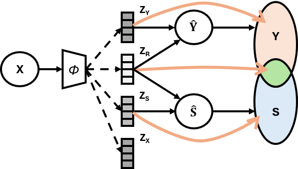
Figure 2: Illustration of the data flow. The orange lines connect the information in the observed space and their corresponding latent codes.

From a causal perspective, if $Y$ and $S$ are conditionally independent given $z_{R}$ (i.e., $Y\perp S\mid z_{R}$), $z_{R}$ effectively serves as the common cause, promoting the independence of $z_{Y}$ and $z_{S}$. Figure 2 illustrates this information flow, demonstrating how $z_{R}$ manages correlated information while maintaining the independence of the other latent codes.

Our fairness objective is to achieve independence between $z_{Y}$ and $z_{S}$ by enforcing conditional independence between $\hat{Y}$ and $\hat{S}$ given $z_{R}$, where: $\hat{Y}\!=\!f_{y}(z_{Y},z_{R})$ and $\hat{S}\!=\!f_{s}(z_{S},z_{R})$. Additionally, we utilize $z_{X}$ as an auxiliary latent code to filter out irrelevant features, allowing for more controlled counterfactual generation.

We first consider enforcing the proposed disentanglement by directly imposing Conditional Independence (CI), namely

$$p_{\theta}(\hat{Y},\hat{S}\mid z_{R})=p_{\theta}(\hat{Y}\mid z_{R})\,p_{\theta}(\hat{S}\mid z_{R}),$$ (7)

which implies $\hat{Y}\,\perp\,\hat{S}\;\big{|}\;z_{R}$. Ideally, one could measure how close $\hat{Y}$ and $\hat{S}$ are to being conditionally independent by minimizing the divergence $D\!\bigl{(}p_{\theta}(\hat{Y},\hat{S}\mid z_{R})\,\big{\|}\,p_{\theta}(\hat{Y}\mid z_{R})\,p_{\theta}(\hat{S}\mid z_{R})\bigr{)}$, but this is generally intractable to compute in practice. Instead, we follow standard information-theoretic principles and propose to minimize the Conditional Mutual Information (CMI): $I_{\phi}(\hat{Y};\hat{S}\mid z_{R})$, as a tractable surrogate objective. By definition of CMI,

$$I_{\phi}(\hat{Y};\hat{S}\mid z_{R})=$$ (8)

$$\int\!D_{\mathrm{KL}}\!\Bigl{(}p_{\theta}(\hat{Y},\hat{S}\!\mid\!z_{R})\,\big{\|}\,p_{\theta}(\hat{Y}\!\mid\!z_{R})\,p_{\theta}(\hat{S}\!\mid\!z_{R})\Bigr{)}\,\!dP_{z_{R}},$$

and thus minimizing $I_{\phi}(\hat{Y};\hat{S}\mid z_{R})$ is equivalent to driving the above divergence to zero. See Appendix A for a detailed proof of the equivalence between vanishing conditional mutual information and conditional independence.

From information theory, we know $I_{\phi}(\hat{Y};\hat{S}\mid z_{R})=I_{\phi}(\hat{S};\hat{Y}\mid z_{R})$, thus, when $I_{\phi}(\hat{Y};\hat{S}\mid z_{R})$ (and equivalently $I_{\phi}(\hat{S};\hat{Y}\mid z_{R})$) is minimized, any undesired dependence between $\hat{Y}$ and $\hat{S}$ is removed.

3.3 Direct Minimization of Conditional Mutual Information

To achieve CI as (7), we propose directly minimizing:

$$\min_{\phi}\Bigl{[}I_{\phi}(\hat{Y};\hat{S}\mid z_{R})+I_{\phi}(\hat{S};\hat{Y}\mid z_{R})\Bigr{]},$$ (9)

where:

$$I_{\phi}(\hat{Y};\hat{S}\mid z_{R})=H_{\phi}(\hat{Y}\mid z_{R})-H_{\phi}(\hat{Y}\mid\hat{S},z_{R}),$$ (10)

$H_{\phi}(*\mid*)$ stands for the conditional entropy. Incorporating $\hat{S}\!=\!f_{s}(z_{S},z_{R})$, we have:

$$I_{\phi}(\hat{Y};\hat{S}\mid z_{R}) =H_{\phi}(\hat{Y}\mid z_{R})-H_{\phi}(\hat{Y}\mid\hat{S},z_{R})$$ (11)

$$=H_{\phi}(\hat{Y}\mid z_{R})-H_{\phi}(\hat{Y}\mid f_{s}(z_{S},z_{R}),z_{R})$$

$$=H_{\phi}(\hat{Y}\mid z_{R})-H_{\phi}(\hat{Y}\mid z_{S},z_{R})$$

$$=I_{\phi}(\hat{Y};z_{S}\mid z_{R}),$$

from the same transformation (see detailed derivation in Appendix B):

$$I_{\phi}(\hat{S};\hat{Y}\mid z_{R}) =I_{\phi}(\hat{S};z_{Y}\mid z_{R})$$

$$=H_{\phi}(\hat{S}\mid z_{R})-H_{\phi}(\hat{S}\mid z_{Y},z_{R}).$$ (12)

Therefore, with the introduction of the correlated latent code $z_{R}$ that captures all relevant information between $\hat{Y}$ and $\hat{S}$:

$$\min_{\phi}\Bigl{[} I_{\phi}(\hat{Y};\hat{S}\mid z_{R})+I_{\phi}(\hat{S};\hat{Y}\mid z_{R})\bigr{]}$$ (13)

$$\equiv\min_{\phi}\Bigl{[}I_{\phi}(\hat{Y};z_{S}\mid z_{R})+I_{\phi}(\hat{S};z_{Y}\mid z_{R})\Bigr{]}.$$

For the minimization of $I_{\phi}(\hat{Y};z_{S}\mid z_{R})$, as shown in (11) , since $z_{R}$ is given as a condition, we can consider this CMI formula as a function where the independent variable is $z_{S}$ and the dependent variable is $\hat{Y}$, as shown as:

$$\mathcal{L}_{\hat{Y}}(z_{S})=H_{\phi}(\hat{Y}\mid z_{R})-H_{\phi}(\hat{Y}\mid z_{S},z_{R}),$$ (14)

where $z_{R}$ is determined here, $H_{\phi}(\hat{Y}\mid z_{R})$ is a constant, henceforth we need to minimize $-H_{\phi}(\hat{Y}\mid z_{S},z_{R})$. Empirically, we directly minimize the lower bound of it: $-H_{\phi}(\hat{Y}\mid z_{S})$, since: $-H_{\phi}(\hat{Y}\mid z_{S},z_{R})\geq-H_{\phi}(\hat{Y}\mid z_{S})$. Symmetrically, the minimization of $I_{\phi}(\hat{S};z_{Y}\mid z_{R})$ shown in (3.3) is the same concept, see Appendix B for detailed derivation. In this optimization process, $z_{R}$ is responsible for containing any correlation information between target attribute $Y$ and sensitive attribute $S$.

After these simplifications, we introduce the CMI loss to minimize (9):

$$\min_{\phi}\Bigl{[}\mathcal{L}_{\text{CMI}}(\omega_{y\_op};\omega_{s\_op};\phi)\Bigr{]}\!\!=\!-(H_{\phi}(\hat{Y}\mid z_{S})+H_{\phi}(\hat{S}\mid z_{Y})),$$ (15)

where only update encoder parameters $\phi$. Utilizing opponent classifier $f_{y\_op}(z_{S})$, the entropy term calculation are shown as below:

$$H_{\phi}(\hat{Y}\mid z_{S}) \!=\!\mathbb{E}_{q_{\phi}(z_{S}\mid x)}\!\biggl{[}-\!\sum_{\,\hat{y}\in\mathcal{Y}}\,\!p_{\theta}(\hat{y}\mid z_{S})\,\!\log\,p_{\theta}(\hat{y}\mid z_{S})\biggr{]}$$ (16)

$$\!=\!\frac{1}{\lvert B\rvert}\,\!\sum_{i=1}^{\lvert B\rvert}\,\!\sum_{\,\hat{y}\in\mathcal{Y}}\,\!\biggl{[}-\!p_{\theta}\bigl{(}\hat{y}\mid z_{S}^{(i)}\bigr{)}\!\log p_{\theta}\bigl{(}\hat{y}\mid z_{S}^{(i)}\bigr{)}\biggr{]},$$

where $p_{\theta}\bigl{(}\hat{y}\mid z_{S}^{(i)}\bigr{)}\!=\!f_{y\_op}\bigl{(}z_{S}^{(i)}\bigr{)}.$ Here, $z_{S}^{(i)}$ denotes the $z_{S}$ sample from the $i$-th element in a mini-batch of size $|B|$; the distribution $q_{\phi}(z_{S}\mid x)$ is given by the encoder. Similar calculation to $H_{\phi}(\hat{S}\mid z_{Y})$, see Appendix C for completed calculation formula. During this optimization process, the opponent classifier parameters $\omega_{y\_op}$ and $\omega_{s\_op}$ are frozen.

3.4 Learning Relevance Between Target And Sensitive Information

To encourage $z_{R}$ capture and only capture the shared information relevant to target property and sensitive property, as well as $z_{Y}$, $z_{S}$ capture main information of $Y$ and $S$ attributes respectively, we propose to maximize the conditional mutual information as Learning Relevance Information loss:

$$\min_{\phi}\Bigl{[}\mathcal{L}_{\text{LRI}}(\omega_{y};\omega_{s};\phi)\Bigr{]}\!=\!-(I_{\phi}(\hat{Y};Y\mid z_{R})+I_{\phi}(\hat{S};S\mid z_{R})),$$ (17)

where:

$$I_{\phi}(\hat{Y};Y\mid z_{R})=H_{\phi}(\hat{Y}\mid z_{R})-H_{\phi}(\hat{Y}\mid Y,z_{R}),$$ (18)

$$I_{\phi}(\hat{S};S\mid z_{R})=H_{\phi}(\hat{S}\mid z_{R})-H_{\phi}(\hat{S}\mid S,z_{R}),$$ (19)

$H_{\phi}(*\mid*)$ stands for the conditional entropy. Maximizing $H_{\phi}(\hat{Y}\mid z_{R})$, $H_{\phi}(\hat{S}\mid z_{R})$ avoid $z_{R}$ capture all information of $Y$ and $S$: $Y\cap S$, which will lead to the Information Bottleneck phenomenon[15, 6, 19] i.e $z_{R}$ capture all the information about target attribute $Y$ and sensitive attribute $S$, degenerating disentanglement performance. On the other hand, minimizing $H_{\phi}(\hat{Y}\mid Y,z_{R})$ and $H_{\phi}(\hat{S}\mid S,z_{R})$ encourage $z_{R}$ capture relevant information between $Y$ and $S$, which is achieved by marginalizing latent codes in different attribute groups as shown in next.

For entropy calculation of $H_{\phi}(\hat{Y}\mid z_{R})$, We approximate $p_{\theta}(\hat{y}\mid z_{R})$ by marginalizing over $z_{Y}$:

$$p_{\theta}(\hat{y}\mid z_{R}^{(k)}) =\mathbb{E}_{p(x)}\left[\mathbb{E}_{q_{\phi}(z_{Y}\mid x)}\left[p_{\theta}(\hat{y}\mid z_{Y},z_{R}^{(k)})\right]\right]$$ (20)

$$\approx\frac{1}{|B|}\sum_{i=1}^{|B|}p_{\theta}(\hat{y}\mid z_{Y}^{(i)},z_{R}^{(k)}),$$

where $p_{\theta}(\hat{y}\mid z_{Y}^{(i)},z_{R}^{(k)})\!=\!f_{y}\bigl{(}z_{Y}^{(i)},z_{R}^{(k)}\bigr{)}$, then

$$H_{\phi}(\hat{Y}\mid z_{R})\!=\!\mathbb{E}_{q_{\phi}(z_{R}\mid x)}\left[-\sum_{\hat{y}\in\mathcal{Y}}p_{\theta}(\hat{y}\mid z_{R})\log p_{\theta}(\hat{y}\mid z_{R})\right]$$ (21)

$$\!=\!\frac{1}{|B|}\sum_{i=1}^{|B|}\sum_{\hat{y}\in\mathcal{Y}}\left[-p_{\theta}(\hat{y}\mid z_{R}^{(i)})\log p_{\theta}(\hat{y}\mid z_{R}^{(i)})\right].$$

As for the calculation of conditional entropy term $H_{\phi}(\hat{Y}\mid Y,z_{R})$, we regard known condition $Y$ as attribute to grouping samples in a mini-batch of size $|B|$, and calculate the entropy term by marginalizing over $z_{Y}$ within each group, $p_{\theta}(\hat{y}\mid z_{R},y)$ can be computed for $z_{R}^{(k)}$ sampled from an instance $x^{(k)}\in B_{y}$ as:

$$p_{\theta}(\hat{y}|z_{R}^{(k)},y) =\mathbb{E}_{p(x\mid Y=y)}\left[\mathbb{E}_{q_{\phi}(z_{Y}\mid x)}\left[p_{\theta}(\hat{y}\mid z_{Y},z_{R}^{(k)})\right]\right]$$ (22)

$$\approx\frac{1}{|B_{y}|}\sum_{i=1}^{|B_{y}|}p_{\theta}(\hat{y}|z_{Y}^{(i)},z_{R}^{(k)}),$$

where $B_{y}$ denotes a subset of the batch with $Y=y$. Then the conditional entropy can be computed as:

$$H_{\phi}(\hat{Y}\mid Y,z_{R})=$$ (23)

$$\mathbb{E}_{(x,y)\sim\mathcal{D}}\!\left[\!\mathbb{E}_{q_{\phi}(z_{R}\mid x)}\!\left[\!-\!\sum_{\hat{y}\in\mathcal{Y}}\!p_{\theta}(\hat{y}\!\mid\!z_{R},y)\!\log p_{\theta}(\hat{y}\!\mid\!z_{R},\!y)\right]\!\right]\!$$

$$=\frac{1}{|B|}\!\sum_{y\in\mathcal{Y}}\!\sum_{i=1}^{|B_{y}|}\!\sum_{\hat{y}\in\mathcal{Y}}\left[-p_{\theta}(\hat{y}|z_{R}^{(i)},y)\!\log p_{\theta}(\hat{y}|z_{R}^{(i)},y)\right].$$

The calculation of $H_{\phi}(\hat{S}\mid z_{R})$ and $H_{\phi}(\hat{S}\mid S,z_{R})$ are similar to $H_{\phi}(\hat{Y}\mid z_{R})$, $H_{\phi}(\hat{Y}\mid Y,z_{R})$ respectively, see Appendix C for completed calculation formula. Plugging these estimates(21)(LABEL:cal_H_Y_Y_zr) back into (17), shared feature between $Y$ and $S$ will be learned in $z_{R}$ while getting rid of Information Bottleneck phenomenon. Note that the classifier parameters $\omega_{y}$ and $\omega_{s}$ are remain freeze when (17) optimizing.

3.5 Final Objective Function

To integrate the above components into a coherent training framework, we employ the two-step optimization strategy defined in (24) and (25).

$$\min_{\theta,\phi,\omega_{y},\omega_{s}}\Bigl{[}\mathcal{L}_{\text{VAE}}(\theta,\phi)+\bigl{(}\mathcal{L}_{y}(\omega_{y},\phi)+\mathcal{L}_{s}(\omega_{s},\phi)\bigr{)}\Bigr{]}\!\!+\!\min_{\phi}\Bigl{[}$$ (24)

$$\lambda_{\text{CMI}}\mathcal{L}_{\text{CMI}}(\omega_{y\_op},\omega_{s\_op};\phi)\!+\!\mathcal{L}_{\text{TC}}(\phi)\!+\!\lambda_{\text{LRI}}\,\mathcal{L}_{\text{LRI}}(\omega_{y},\omega_{s};\phi)\Bigr{]}$$

Specifically, in (24), we jointly update $(\theta,\phi,\omega_{y},\omega_{s})$ by minimizing the VAE loss (2) alongside the main classification losses (3) and (4), which together reformulate the ELBO. We further include the CMI loss (15) to reduce unwanted information leakage, the LRI loss (17) to capture shared patterns in $z_{R}$, and the TC penalty (1) to promote factorization among the latent codes $(z_{Y},z_{R},z_{S})$.

$$\min_{\omega_{y\_op},\omega_{s\_op}}\Bigl{[}\mathcal{L}_{y\_op}(\omega_{y\_op};\phi)+\mathcal{L}_{s\_op}(\omega_{s\_op};\phi)\Bigr{]}$$ (25)

In parallel, the second procedure (25) optimizes $(\omega_{y\_op},\omega_{s\_op})$ by minimizing the opponent classification losses (5) and (6) while holding $\phi$ fixed.

The hyperparameters $\lambda_{CMI},\lambda_{LRI}>0$ control the relative importance of these terms, ensuring each network component learns its designated function while enforcing minimal information leakage, preserving shared information in $z_{R}$ and maintaining the salient factors for $Y$ and $S$ in $z_{Y}$ and $z_{S}$ respectively. See hypermeter analysis in Appendix D.

4 Experiment

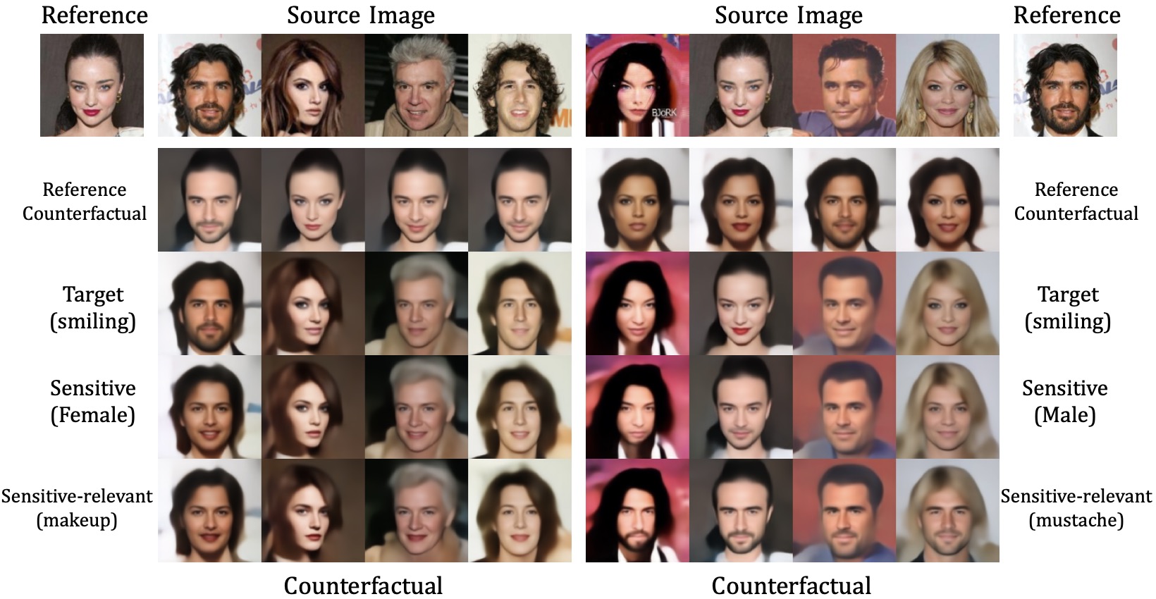
Figure 3: Examples of Fair Counterfactual Generation. The first row shows the source and reference images. Rows 2–5 display counterfactuals obtained by replacing latent subspaces $z_{X}$, $z_{Y}$, $z_{S}$, and $[z_{S},z_{R}]$, respectively. Notably, the replacement with $[z_{S},z_{R}]$ (row 5) naturally adapts sensitive features for different sensitive attributes without domain knowledge. (mustache for men and makeup for women).

To ensure a rigorous and comprehensive evaluation, we conduct experiments comparing our proposed method with a diverse set of state-of-the-art approaches across multiple categories of learning paradigms in various tasks. Specifically, we include FairFactorVAE [28], FairDisCo [27], FFVAE [6], GVAE [7], ODVAE [42] and FADES [15], shown in Section 2.1. As for traditional correlation-aware learning that is discussed in Section 2.2, since it require additional annotated data to build causal graph, we except them in our experiment. Further details on the experimental setup and additional discussions are provided in Appendix D.

4.1 Fair Classification

Table 1: Evaluation of downstream classification tasks on various datasets from learned representation. Best in bold, second in red.

                 Downstream Classification Performance Methods CelebA [29] UTKFace [49] Dogs and Cats [37] Color bias MNIST [17] Acc $\uparrow$ EOD $\downarrow$ DP $\downarrow$ Acc $\uparrow$ EOD $\downarrow$ DP $\downarrow$ Acc $\uparrow$ EOD $\downarrow$ DP $\downarrow$ Acc $\uparrow$ EOD $\downarrow$ DP $\downarrow$   FADES [15] [CVPR’24] 0.918 0.034 0.135 0.812 0.059 0.139 0.769 0.058 0.086 0.973 0.094 0.160 GVAE [7] [CVPR’20] 0.919 0.047 0.131 0.819 0.204 0.197 0.748 0.064 0.131 0.961 0.109 0.176 FFVAE [6] [PMLR’19] 0.892 0.076 0.072 0.766 0.269 0.201 0.729 0.059 0.110 0.952 0.081 0.092 ODVAE [42] [ECCV’20] 0.886 0.039 0.103 0.736 0.165 0.210 0.689 0.051 0.038 0.957 0.247 0.162 FairDisCo [27] [KDD’22] 0.839 0.074 0.051 0.766 0.266 0.200 0.680 0.115 0.111 0.949 0.129 0.136 FairFactorVAE [28] 0.914 0.055 0.136 0.720 0.096 0.134 0.707 0.055 0.110 0.957 0.096 0.128 CAD-VAE (Ours) 0.923 0.021 0.112 0.817 0.045 0.137 0.773 0.048 0.090 0.977 0.076 0.118  

The objective of fair classification is to achieve a balance between minimizing fairness violations and maintaining high predictive performance. To evaluate the effectiveness of our proposed method, we conduct experiments on a diverse set of benchmark fairness datasets. For facial attribute classification tasks, we utilize the CelebA [29] and UTKFace [49] datasets. Following prior works [44, 47, 48, 15], we set the CelebA classification task to predict the “Smiling” attribute, while for UTKFace, the objective is to classify whether a person depicted in the image is over 35 years old, with gender serving as the sensitive attribute. Additionally, the Dogs and Cats dataset [37] is used to distinguish between dogs and cats, with fur color as the sensitive attribute. Furthermore, we assess fair classification performance using the Colored MNIST dataset [18, 17, 35], which incorporates a controlled color bias in the standard MNIST dataset to simulate spurious correlations. To assess fairness violations, we use standard metrics including Demographic Parity (DP) [2] and Equalized Odds (EOD) [10]. See detailed experimental setup in Appendix D.

The result of fair classification can be seen in Table 1. Across all evaluated datasets, our method consistently achieves state-of-the-art classification accuracy and fairness, validating its effectiveness in robust disentanglement by preserving high-quality target-related information while minimizing sensitive attribute leakage. Among the baselines, FADES achieves competitive accuracy and strong fairness. However, its inability to strictly minimize conditional mutual information results in sensitive information leakage and an excessive capture of target-related data in the relevance latent code $z_{R}$, which limits classification performance. In contrast, our approach directly minimizes the conditional mutual information between $z_{Y}$ and $z_{S}$ regarding their respective opposite attributes $S$ and $Y$, and incorporates an explicit relevance learning strategy, as detailed in Section 3.3 and Section 3.4. This design ensures that $z_{R}$ captures sufficient, but not excessive, information about $Y$ and $S$, thereby enhancing fairness while preserving essential target information. More fair classification experiment results can be seen in Appendix E.

4.2 Fair Counterfactual Generation

We evaluate our approach on the CelebA dataset [29], a widely-used benchmark for facial attribute manipulation. We select Smiling as the target label $Y$ and Gender as the sensitive attribute $S$. In our experiments, we substitute specific latent code of source images with reference images, including $z_{X}$, $z_{Y}$, $z_{S}$, and $[z_{S},z_{R}]$. Figure 3 illustrates the generated counterfactuals, with the first row showing source and reference images and subsequent rows demonstrating the effects of substituting each latent code.

The experimental results demonstrate the effectiveness of our method in generating fair counterfactuals. As shown in Figure 3, substituting $[z_{S},z_{R}]$ (Row 5) leads to a natural adaptation of sensitive-relevant features without domain-specific knowledge. For instance, the model automatically adds makeup to female images and a mustache to male images, highlighting the semantic alignment of $z_{R}$ with both the target and sensitive attributes. Compared to substituting only $z_{S}$, our approach achieves more interpretable translation, ensuring that fairness is maintained throughout the counterfactual generation. More fair counterfactual generation experiment results can be seen in Appendix E.

To quantitatively assess the quality of the generated counterfactuals, we compare evaluation metrics between the direct reconstruction of the input image and the reconstructions obtained by randomly permuting $z_{Y}$ and $z_{S}$ within the evaluation set. Specifically, we use the FID [12, 15] to assess reconstruction fidelity and the Inception Score (IS) [5] to evaluate semantic and perceptual quality. Lower $\Delta\text{FID}$ values indicate minimal distortion and higher translation quality, while lower $\Delta\text{IS}$ values suggest that semantic and perceptual attributes are well preserved. Detailed experimental settings are provided in Appendix D.

Table 2: FID and IS difference between original reconstruction and perturbed target/sensitive codes’ reconstruction.

  CAD-VAE FADES GVAE FFVAE ODVAE FairFactorVAE $\Delta\textit{\text{FID}}\downarrow$ 1.072 1.167 3.710 1.409 14.647 6.239 $\Delta\textit{\text{IS}}\downarrow$ 1.214 2.379 3.148 3.829 6.113 5.378  

Quantitative analysis in Table 2 further validates our approach. Our method achieves both lower $\Delta\text{FID}$ and $\Delta\text{IS}$ compared to other fair representation learning methods, demonstrating that our fair counterfactual generation approach renders counterfactuals with superior image quality and minimal distortion.

4.3 Fair Fine-Grained Image Editing

With the introduction of the correlated latent code $z_{R}$, fair fine-grained image editing—as a fundamental concept in counterfactual fairness—can be naturally achieved by aligning latent codes from different samples. We use linear interpolation to synthesize a latent code: $z^{\prime}=(1-\lambda)z_{1}+\lambda z_{2}$, where $z_{1}$ is the latent code from the source image and $z_{2}$ is the corresponding code from the reference image. The synthesized $z^{\prime}$ replaces $z_{1}$, enabling a gradual transfer from the source to the reference latent code.

In our experiments, following the setup in Section 4.2 where Smiling is the target label $Y$ and Gender is the sensitive attribute $S$, we generate interpolated latent codes between source and reference images. In the blue-framed subfigure of Figure 1, images are generated by interpolating $z_{Y}$ and $z_{S}$: the horizontal axis shows the transition of $z_{S}$ from the source to the reference image, while the vertical axis shows the corresponding change in $z_{Y}$. During this interpolation, $z_{R}$ and $z_{X}$ remain unchanged, with the interpolation parameters for both $z_{Y}$ and $z_{S}$ set to $\lambda\in\{0,0.33,0.66,1\}$.

Similarly, in the red-framed subfigure, images are generated by interpolating $z_{Y}$ and $z_{R}$. Here, the horizontal axis corresponds to the transition of $z_{R}$ from the source to the reference image, and the vertical axis corresponds to $z_{Y}$. Note that the source image’s $z_{S}$ is fully replaced by that of the reference image, and $z_{X}$ remains constant. Initially, the interpolation parameters for $z_{R}$ are set to $\lambda\in\{0.5,1\}$, and when combined with the final column of the blue-framed subfigure, the range is extended to $\lambda\in\{0,0.5,1\}$.

Figure 1 demonstrates a smooth transformation of each attribute, with modifications in one latent code minimally affecting the others, a key characteristic of effective disentanglement. Specifically, as the correlated latent code $z_{R}$ captures sensitive relevant information, we can explicitly control these properties: in the left subfigure, we gradually introduce makeup (such as enhanced lipstick and eyeshadow), while in the right subfigure, we progressively add a mustache. More fair fine-grained image editing experiment results can be seen in Appendix E.

Similarly, we measure $\Delta\text{FID}$ and $\Delta\text{IS}$ to quantitatively assess the quality of fine-grained image editing. Unlike the evaluation setup in Section 4.2, we compute the differences in evaluation metrics between the direct reconstruction of the input image and the reconstructions obtained through latent code traversals for each $\lambda$ combination. Detailed experimental settings are provided in Appendix D. Table 3 summarizes the comparison results, showing that our method exhibits both lower $\Delta\text{FID}$ and $\Delta\text{IS}$ values compared to other fair generation methods. These results indicate that our fine-grained image editing approach not only ensures smoother attribute transformations and superior image fidelity, but also allows for more precise control of task-relevant features.

4.4 Fair Text-to-Image Editing

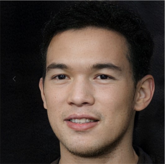
(a) Original

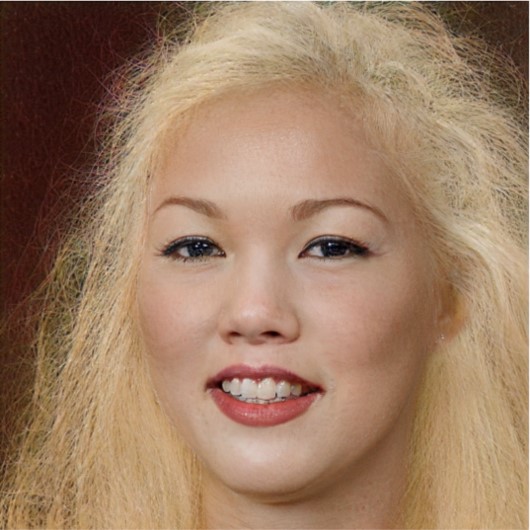
(b) StyleCLIP

(c) StyleCLIP+

Figure 4: Style transfer using StyleCLIP and the CAD-VAE extension. This example transforms the (a) into “a dancer with long blonde hair.” “StyleCLIP+” means StyleCLIP + CAD-VAE.

To further validate the capability and explore the applicability of our method, we integrated it as an adaptor on top of a pre-trained, frozen CLIP image encoder [39] and trained it on Facet dataset [9] to enhance fairness in vision-language tasks. Table 4 presents the experimental results. These results demonstrate that our approach significantly improves fairness without compromising performance compared to the linear probing baseline (ERM), underscoring its potential for a range of vision-language tasks with fairness considerations.

Furthermore, we applied our method in StyleCLIP [38] as a fair discriminator to address inherent fairness issues, such as career-gender biases, which persist even when an identity preservation loss is employed. As illustrated in Figure 8, StyleCLIP [38] exhibits a bias by correlating the role of “dancer” with a specific gender. In contrast, our method effectively mitigates this bias while maintaining the efficacy of attribute modification. See Appendix E for details.

Table 3: FID and IS difference between original reconstruction and traversed target/sensitive codes’ reconstruction.

  CAD-VAE FADES GVAE FFVAE ODVAE FairFactorVAE $\Delta\textit{\text{FID}}\downarrow$ 1.642 2.362 4.023 2.789 15.893 7.120 $\Delta\textit{\text{IS}}\downarrow$ 1.849 2.919 4.848 5.292 6.890 5.767  

Table 4: Performance of CLIP(ViTB/32) on Facet dataset. WG: Worst Group, Gap: Difference between WG and Avg.

  Method Top-1 Acc. (%) Top-3 Acc. (%) WG $\uparrow$ Avg $\uparrow$ Gap $\downarrow$ WG $\uparrow$ Avg $\uparrow$ Gap $\downarrow$   Zero-shot 2.79 53.45 50.66 15.31 76.79 61.48 Linear prob 1.17 65.46 64.29 1.79 85.34 83.55 CAD-VAE 69.97 70.54 0.57 85.36 85.95 0.59  

5 Conclusion

Our method aims to solve fairness concerns in representation learning and deep generative models. By introducing a correlated latent code that captures shared information, sensitive information leakage can be eliminated directly and efficiently without conflicting with the prediction objective, which is a core issue in disentanglement, by minimizing the conditional mutual information between target latent code and sensitive latent code. Parallel with our explicit relevance learning strategy imposed on the correlated latent code, it is encouraged to capture the essential shared information that cannot be perfectly separated without additional domain knowledge. Various benchmark tasks further demonstrate the robustness and wide applicability of our method. Further details on the experimental setup, results, discussion, and potential future directions are provided in the Appendix.

6 Relation between Conditional Mutual Information and Conditional Independence

Proposition 1

Let $X,Y,Z$ be random variables with a joint distribution $P_{X,Y,Z}$. Then the following are equivalent:

1. $I(X;Y\mid Z)=0$,

2. $X$ and $Y$ are conditionally independent given $Z$, i.e., $X\perp Y\mid Z$.

(2) $\implies$ (1). If $X$ is conditionally independent of $Y$ given $Z$, we have

$$P_{X,Y|Z}(x,y\mid z)\;=\;P_{X|Z}(x\mid z)\,P_{Y|Z}(y\mid z).$$ (26)

Thus, for each $z$ with $P_{Z}(z)>0$,

$$\log\!\biggl{[}\frac{P_{X,Y|Z}(x,y\mid z)}{P_{X|Z}(x\mid z)\,P_{Y|Z}(y\mid z)}\biggr{]}\;=\;\log(1)\;=\;0.$$ (27)

Therefore,

$$I(X;Y\!\mid\!Z)$$ (28)

$$=\!\!\sum_{z}\!P_{Z}(z)\!\sum_{x,y}\!P_{X,Y\mid Z}(x,y\!\mid\!z)\!\log\!\biggl{[}\frac{P_{X,Y|Z}(x,y\!\mid\!z)}{P_{X|Z}(x\!\mid\!z)\,P_{Y|Z}(y\!\mid\!z)}\!\biggr{]}$$

$$=0.$$

(1) $\implies$ (2). Suppose $I(X;Y\mid Z)=0$. Define

$$F(x,y)\;:=\;\frac{P_{X|Z}(x\mid z)\,P_{Y|Z}(y\mid z)}{P_{X,Y|Z}(x,y\mid z)},$$ (29)

for each $z$ such that $P_{Z}(z)>0$. A direct calculation shows

$$\sum_{x,y}P_{X,Y|Z}(x,y\mid z)\;F(x,y)$$ (30)

$$\!=\!\sum_{x,y}P_{X|Z}(x\mid z)\,P_{Y|Z}(y\mid z)\!=\!1.$$

The conditional mutual information can be written as

$$I(X;Y\!\mid\!Z)$$ (31)

$$=\!\!\sum_{z}\!P_{Z}(z)\!\sum_{x,y}\!P_{X,Y\mid Z}(x,y\!\mid\!z)\!\log\!\biggl{[}\frac{P_{X,Y|Z}(x,y\!\mid\!z)}{P_{X|Z}(x\!\mid\!z)\,P_{Y|Z}(y\!\mid\!z)}\!\biggr{]}$$

$$=-\,\sum_{z}P_{Z}(z)\sum_{x,y}P_{X,Y|Z}(x,y\mid z)\,\log F(x,y).$$

Using the identity

$$\!-\!\,\!\log F(x,y)\!=\!\bigl{[}F(x,y)\!-\!1\!-\!\log F(x,y)\bigr{]}\!-\!\bigl{[}F(x,y)\!-\!1\bigr{]},$$ (32)

and rearranging, one obtains

$$I(X;Y\mid Z)$$ (33)

$$=\!\sum_{z}\!P_{Z}(z)\!\sum_{x,y}\!P_{X,Y|Z}(x,y\!\mid\!z)\!\Bigl{[}F(x,y)\!-\!1\!-\!\log\!F(x,y)\Bigr{]}\!.$$

To see why this rearrangement holds, substitute the above identity into $\sum_{x,y}P_{X,Y|Z}(x,y\mid z)\,\log F(x,y)$. The result is a difference of two sums; one of these sums, $\sum_{x,y}P_{X,Y|Z}(x,y\mid z)\,\bigl{[}F(x,y)-1\bigr{]}$, is zero because

$$\sum_{x,y}P_{X,Y|Z}(x,y\mid z)\,\bigl{[}F(x,y)-1\bigr{]}$$ (34)

$$\;=\;\sum_{x,y}P_{X,Y|Z}(x,y\mid z)\,F(x,y)\!-\!\sum_{x,y}P_{X,Y|Z}(x,y\mid z)$$

$$\;=\;1-1=0.$$

Hence we arrive at the above expression for (33).

Since $\log t\leq t-1$ for all $t>0$, we have

$$F(x,y)-1-\log F(x,y)\;\geq\;0,$$ (35)

and hence each summand in the expression for $I(X;Y\mid Z)$ is nonnegative. Because $I(X;Y\mid Z)=0$ by hypothesis, it must be that

$$F(x,y)-1-\log F(x,y)\;=\;0\quad\text{for all $x,y$},$$ (36)

implying $F(x,y)=1$. Therefore,

$$F(x,y)=\frac{P_{X|Z}(x\mid z)\,P_{Y|Z}(y\mid z)}{P_{X,Y|Z}(x,y\mid z)}\;=\;1,$$ (37)

so that

$$P_{X,Y|Z}(x,y\mid z)\;=\;P_{X|Z}(x\mid z)\,P_{Y|Z}(y\mid z).$$ (38)

This is precisely the definition of conditional independence: $X\perp Y\mid Z$.

Since we have shown both directions $\textbf{(2)}\implies\textbf{(1)}$ and $\textbf{(1)}\implies\textbf{(2)}$, the proof is complete.

7 Complete Transformation Process of Conditional Mutual Information

$H_{\phi}(*\mid*)$ stand the conditional entropy, and

$$\hat{Y}=f_{y}(z_{Y},z_{R})$$ (39)

$$\hat{S}=f_{s}(z_{S},z_{R}).$$ (40)

Incorporating (40), we have:

$$I_{\phi}(\hat{Y};\hat{S}\mid z_{R}) =H_{\phi}(\hat{Y}\mid z_{R})-H_{\phi}(\hat{Y}\mid\hat{S},z_{R})$$ (41)

$$=H_{\phi}(\hat{Y}\mid z_{R})-H_{\phi}(\hat{Y}\mid f_{s}(z_{S},z_{R}),z_{R})$$

$$=H_{\phi}(\hat{Y}\mid z_{R})-H_{\phi}(\hat{Y}\mid z_{S},z_{R})$$

$$=I_{\phi}(\hat{Y};z_{S}\mid z_{R}).$$

Incorporating (39), we have:

$$I_{\phi}(\hat{S};\hat{Y}\mid z_{R}) =H_{\phi}(\hat{S}\mid z_{R})-H_{\phi}(\hat{S}\mid\hat{Y},z_{R})$$ (42)

$$=H_{\phi}(\hat{S}\mid z_{R})-H_{\phi}(\hat{S}\mid f_{y}(z_{Y},z_{R}),z_{R})$$

$$=H_{\phi}(\hat{S}\mid z_{R})-H_{\phi}(\hat{S}\mid z_{Y},z_{R})$$

$$=I_{\phi}(\hat{S};z_{Y}\mid z_{R}).$$

Therefore, with the introduction of the correlated latent code $z_{R}$ that captures all relevant information between $\hat{Y}$ and $\hat{S}$:

$$\min_{\phi}\Bigl{[} I_{\phi}(\hat{Y};\hat{S}\mid z_{R})+I_{\phi}(\hat{S};\hat{Y}\mid z_{R})\bigr{]}$$ (43)

$$\equiv\min_{\phi}\Bigl{[}I_{\phi}(\hat{Y};z_{S}\mid z_{R})+I_{\phi}(\hat{S};z_{Y}\mid z_{R})\Bigr{]}.$$

For the minimization of $I_{\phi}(\hat{Y};z_{S}\mid z_{R})$, as shown in (41), since $z_{R}$ is given as a condition, we can consider this CMI formula as a function where the independent variable is $z_{S}$ and the dependent variable is $\hat{Y}$, as shown as:

$$\mathcal{L}_{\hat{Y}}(z_{S})=H_{\phi}(\hat{Y}\mid z_{R})-H_{\phi}(\hat{Y}\mid z_{S},z_{R}),$$ (44)

where $z_{R}$ is determined here, $H_{\phi}(\hat{Y}\mid z_{R})$ is a constant, henceforth we need to minimize $-H_{\phi}(\hat{Y}\mid z_{S},z_{R})$. Empirically, we directly minimize the lower bound of it: $-H_{\phi}(\hat{Y}\mid z_{S})$, since: $-H_{\phi}(\hat{Y}\mid z_{S},z_{R})\geq-H_{\phi}(\hat{Y}\mid z_{S})$.

For the minimization of $I_{\phi}(\hat{S};z_{Y}\mid z_{R})$, as shown in (42), since $z_{R}$ is given as a condition, we can consider this CMI formula as a function where the independent variable is $z_{Y}$ and the dependent variable is $\hat{S}$, as shown as:

$$\mathcal{L}_{\hat{S}}(z_{Y})=H_{\phi}(\hat{S}\mid z_{R})-H_{\phi}(\hat{S}\mid z_{Y},z_{R}),$$ (45)

where $z_{R}$ is determined here, $H_{\phi}(\hat{S}\mid z_{R})$ is a constant, henceforth we need to minimize $-H_{\phi}(\hat{S}\mid z_{Y},z_{R})$. Empirically, we directly minimize the lower bound of it: $-H_{\phi}(\hat{S}\mid z_{Y})$, since: $-H_{\phi}(\hat{S}\mid z_{Y},z_{R})\geq-H_{\phi}(\hat{S}\mid z_{Y})$.

After these simplifications, we can introduce the CMI loss to minimize (43):

$$\min_{\phi}\Bigl{[}\mathcal{L}_{\text{CMI}}(\omega_{y\_op};\omega_{s\_op};\phi)\Bigr{]}\!\!=\!-(H_{\phi}(\hat{Y}\mid z_{S})+H_{\phi}(\hat{S}\mid z_{Y})),$$ (46)

where only update encoder parameters $\phi$.

8 Complete Calculation Formula of Entropy Term mentioned in Main Paper

1. $H_{\phi}(\hat{Y}\mid z_{S})$: We use the opponent classifier $f_{y\_op}(z_{S})$, which predicts $y$ from $z_{S}$. Denoting

$$p_{\theta}\bigl{(}\hat{y}\mid z_{S}^{(k)}\bigr{)}\;=\;f_{y\_op}\bigl{(}z_{S}^{(k)}\bigr{)},$$

then

$$H_{\phi}(\hat{Y}\mid z_{S})$$ (47)

$$\;=\;\mathbb{E}_{q_{\phi}(z_{S}\mid x)}\biggl{[}-\sum_{\,\hat{y}\in\mathcal{Y}}\,p_{\theta}(\hat{y}\mid z_{S})\,\log\,p_{\theta}(\hat{y}\mid z_{S})\biggr{]}$$

$$\;=\;\frac{1}{\lvert B\rvert}\,\sum_{i=1}^{\lvert B\rvert}\,\sum_{\,\hat{y}\in\mathcal{Y}}\,\biggl{[}-p_{\theta}\bigl{(}\hat{y}\mid z_{S}^{(i)}\bigr{)}\log p_{\theta}\bigl{(}\hat{y}\mid z_{S}^{(i)}\bigr{)}\biggr{]}.$$

Here, $z_{S}^{(i)}$ denotes the $z_{S}$ sample from the $i$-th element in a mini-batch of size $|B|$; the distribution $q_{\phi}(z_{S}\mid x)$ is given by the encoder.

2. $H_{\phi}(\hat{S}\mid z_{Y})$: Similarly, we employ the opponent classifier $f_{s\_op}(z_{Y})$ to measure how much $z_{Y}$ retains information about $s$. We define

$$p_{\theta}\bigl{(}\hat{s}\mid z_{Y}^{(k)}\bigr{)}\;=\;f_{s\_op}\bigl{(}z_{Y}^{(k)}\bigr{)},$$

and

$$H_{\phi}(\hat{S}\mid z_{Y})$$ (48)

$$\;=\;\mathbb{E}_{q_{\phi}(z_{Y}\mid x)}\biggl{[}-\sum_{\,\hat{s}\in\mathcal{S}}\,p_{\theta}(\hat{s}\mid z_{Y})\,\log\,p_{\theta}(\hat{s}\mid z_{Y})\biggr{]}$$

$$\;=\;\frac{1}{\lvert B\rvert}\,\sum_{i=1}^{\lvert B\rvert}\,\sum_{\,\hat{s}\in\mathcal{S}}\,\biggl{[}-p_{\theta}\bigl{(}\hat{s}\mid z_{Y}^{(i)}\bigr{)}\log p_{\theta}\bigl{(}\hat{s}\mid z_{Y}^{(i)}\bigr{)}\biggr{]}.$$

Here, $z_{Y}^{(i)}$ denotes the $z_{Y}$ sample from the $i$-th element in a mini-batch of size $|B|$; the distribution $q_{\phi}(z_{Y}\mid x)$ is given by the encoder.

3. $H_{\phi}(\hat{Y}\mid z_{R})$: We approximate $p_{\theta}(\hat{y}\mid z_{R})$ by marginalizing over $z_{Y}$:

$$p_{\theta}(\hat{y}\mid z_{R}^{(k)}) =\mathbb{E}_{p(x)}\left[\mathbb{E}_{q_{\phi}(z_{Y}\mid x)}\left[p_{\theta}(\hat{y}\mid z_{Y},z_{R}^{(k)})\right]\right]$$ (49)

$$\approx\frac{1}{|B|}\sum_{i=1}^{|B|}p_{\theta}(\hat{y}\mid z_{Y}^{(i)},z_{R}^{(k)}),$$

where $p_{\theta}(\hat{y}\mid z_{Y}^{(i)},z_{R}^{(k)})$ is obtained by $f_{y}(z_{Y},z_{R})$:

$$p_{\theta}(\hat{y}\mid z_{Y}^{(i)},z_{R}^{(k)})\;=\;f_{y}\bigl{(}z_{Y}^{(i)},z_{R}^{(k)}\bigr{)},$$ (50)

then

$$H_{\phi}(\hat{Y}\mid z_{R})$$ (51)

$$=\mathbb{E}_{q_{\phi}(z_{R}\mid x)}\left[-\sum_{\hat{y}\in\mathcal{Y}}p_{\theta}(\hat{y}\mid z_{R})\log p_{\theta}(\hat{y}\mid z_{R})\right]$$

$$=\frac{1}{|B|}\sum_{i=1}^{|B|}\sum_{\hat{y}\in\mathcal{Y}}\left[-p_{\theta}(\hat{y}\mid z_{R}^{(i)})\log p_{\theta}(\hat{y}\mid z_{R}^{(i)})\right],$$

4. $H_{\phi}(\hat{S}\mid z_{R})$: We approximate $p_{\theta}(\hat{s}\mid z_{R})$ by marginalizing over $z_{S}$:

$$p_{\theta}(\hat{s}\mid z_{R}^{(k)}) =\mathbb{E}_{p(x)}\left[\mathbb{E}_{q_{\phi}(z_{S}\mid x)}\left[p_{\theta}(\hat{s}\mid z_{S},z_{R}^{(k)})\right]\right]$$ (52)

$$\approx\frac{1}{|B|}\sum_{i=1}^{|B|}p_{\theta}(\hat{s}\mid z_{S}^{(i)},z_{R}^{(k)}),$$

where $p_{\theta}(\hat{s}\mid z_{S}^{(i)},z_{R}^{(k)})$ is obtained by $f_{s}(z_{S},z_{R})$:

$$p_{\theta}(\hat{s}\mid z_{S}^{(i)},z_{R}^{(k)})\;=\;f_{s}\bigl{(}z_{S}^{(i)},z_{R}^{(k)}\bigr{)},$$ (53)

then

$$H_{\phi}(\hat{S}\mid z_{R})$$ (54)

$$=\mathbb{E}_{q_{\phi}(z_{R}\mid x)}\left[-\sum_{\hat{s}\in\mathcal{S}}p_{\theta}(\hat{s}\mid z_{R})\log p_{\theta}(\hat{s}\mid z_{R})\right]$$

$$=\frac{1}{|B|}\sum_{i=1}^{|B|}\sum_{\hat{s}\in\mathcal{S}}\left[-p_{\theta}(\hat{s}\mid z_{R}^{(i)})\log p_{\theta}(\hat{s}\mid z_{R}^{(i)})\right],$$

5. $H_{\phi}(\hat{Y}\mid Y,z_{R})$: $p_{\theta}(\hat{y}\mid z_{R},y)$ can be computed for $z_{R}^{(k)}$ sampled from an instance $x^{(k)}\in B_{y}$ as:

$$p_{\theta}(\hat{y}|z_{R}^{(k)},y) =\mathbb{E}_{p(x\mid Y=y)}\left[\mathbb{E}_{q_{\phi}(z_{Y}\mid x)}\left[p_{\theta}(\hat{y}\mid z_{Y},z_{R}^{(k)})\right]\right]$$ (55)

$$\approx\frac{1}{|B_{y}|}\sum_{i=1}^{|B_{y}|}p_{\theta}(\hat{y}|z_{Y}^{(i)},z_{R}^{(k)}),$$

where $B_{y}$ denotes a subset of the batch with $Y=y$. Then the conditional entropy can be computed as:

$$H_{\phi}(\hat{Y}\mid Y,z_{R})=$$ (56)

$$\mathbb{E}_{(x,y)\sim\mathcal{D}}\!\left[\!\mathbb{E}_{q_{\phi}(z_{R}\mid x)}\!\left[\!-\!\sum_{\hat{y}\in\mathcal{Y}}\!p_{\theta}(\hat{y}\!\mid\!z_{R},y)\!\log p_{\theta}(\hat{y}\!\mid\!z_{R},\!y)\right]\!\right]\!$$

$$=\frac{1}{|B|}\!\sum_{y\in\mathcal{Y}}\!\sum_{i=1}^{|B_{y}|}\!\sum_{\hat{y}\in\mathcal{Y}}\left[-p_{\theta}(\hat{y}|z_{R}^{(i)},y)\!\log p_{\theta}(\hat{y}|z_{R}^{(i)},y)\right].$$

6. $H_{\phi}(\hat{S}\mid S,z_{R})$: $p_{\theta}(\hat{s}\mid z_{R},s)$ can be computed for $z_{R}^{(k)}$ sampled from an instance $x^{(k)}\in B_{s}$ as:

$$p_{\theta}(\hat{s}|z_{R}^{(k)},s) =\mathbb{E}_{p(x\mid S=s)}\left[\mathbb{E}_{q_{\phi}(z_{S}\mid x)}\left[p_{\theta}(\hat{s}\mid z_{S},z_{R}^{(k)})\right]\right]$$ (57)

$$\approx\frac{1}{|B_{s}|}\sum_{i=1}^{|B_{s}|}p_{\theta}(\hat{s}|z_{S}^{(i)},z_{R}^{(k)}),$$

where $B_{s}$ denotes a subset of the batch with $S=s$. Then the conditional entropy can be computed as:

$$H_{\phi}(\hat{S}\mid S,z_{R})=$$ (58)

$$\mathbb{E}_{(x,s)\sim\mathcal{D}}\!\left[\!\mathbb{E}_{q_{\phi}(z_{R}\mid x)}\!\left[\!-\!\sum_{\hat{s}\in\mathcal{S}}\!p_{\theta}(\hat{s}\!\mid\!z_{R},s)\!\log p_{\theta}(\hat{s}\!\mid\!z_{R},\!s)\right]\!\right]\!$$

$$=\frac{1}{|B|}\!\sum_{s\in\mathcal{S}}\!\sum_{i=1}^{|B_{s}|}\!\sum_{\hat{s}\in\mathcal{S}}\left[-p_{\theta}(\hat{s}|z_{R}^{(i)},s)\!\log p_{\theta}(\hat{s}|z_{R}^{(i)},s)\right].$$

9 Experiment Setup Details

9.1 Comparison Methods

Specifically, we include FairFactorVAE [19] and FairDisCo [27], both of which leverage invariant learning techniques to encode latent representations that remain independent of sensitive attributes. Additionally, FFVAE [6] employs a mutual information minimization strategy to effectively disentangle latent subspaces. GVAE [7] takes a distinct approach by minimizing information leakage to achieve fair representation learning. ODVAE [42], in contrast, introduces a non-adversarial learning framework that enforces orthogonal priors on the latent subspace, promoting fairness without adversarial training. Finally, FADES [15] proposes minimizing conditional mutual information to achieve fairness, aligning closely with our method. As for traditional correlation-aware learning that discussed in Section 2.2, since it require additional annotated data to build casual graph, we except them in our experiment.

To ensure a fair comparison, we adopt a grid search strategy to fine-tune the hyperparameters of all methods, optimizing for Equalized Odds (EOD) [10]. Specifically, for our method, hyperparameters are explored within the ranges: $\lambda_{CMI}\!\in\![0,10]$ and $\lambda_{LRI}\!\in\![0,100]$. We maintain a consistent architectural setup across all methods, utilizing a ResNet-18 backbone [11] with 512 latent dimensions for all tasks.

9.2 Dimension of each latent code

In our experiment, we set equal dimensional sizes for $z_{Y},z_{S},z_{R}\in\mathbb{R}^{d}$, with $d$ set as a power of 2. Through empirical selection via grid search, we determined $d=32$ for the reported results. Notably, the total latent dimension was fixed at $\mathbb{R}^{512}$ across all methods. Consequently, in our approach, we allocated $z_{X}\in\mathbb{R}^{512-3\times 32}=\mathbb{R}^{416}$. Our empirical findings revealed that setting $d$ beyond 64 led to a decline in reconstruction performance. This degradation likely stems from an excessive allocation of information to each subspace, ultimately compromising the model’s reconstructive capacity.

9.3 Hypermeter Analysis

We evaluated the effect of the two hyperparameters, $\lambda_{CMI}\in[0,10]$ and $\lambda_{LRI}\in[0,100]$, on both classification accuracy and fairness violation (measured as Equalized Odds Difference, EOD) in the CelebA dataset classification task. For the analysis of $\lambda_{CMI}$, we fixed $\lambda_{LRI}$ at 60, while for the analysis of $\lambda_{LRI}$, we fixed $\lambda_{CMI}$ at 5. The result can be seen in Figure 5.

Specifically, $\lambda_{CMI}$ governs the degree to which the conditional mutual information (CMI) loss is minimized. When $\lambda_{CMI}\leq 5$, we observed a modest increase in accuracy as the hyperparameter increases, accompanied by a uniformly decreasing trend in fairness violation. However, when $\lambda_{CMI}>5$, further increments in $\lambda_{CMI}$ lead to a decline in accuracy, even though the fairness violation continues to decrease. This behavior suggests that a moderate level of CMI minimization is beneficial in eliminating unwanted information from the latent code, yet an excessive emphasis on minimizing mutual information may inadvertently remove essential target information from $z_{Y}$.

Similarly, $\lambda_{LRI}$, which regulates the extent to which the latent code $z_{R}$ captures correlated information, exhibits a comparable pattern. For $\lambda_{LRI}\leq 60$, an increase in $\lambda_{LRI}$ results in an improvement in accuracy and a consistent reduction in fairness violation, indicating that a controlled increase enables $z_{R}$ to capture sufficient shared patterns while mitigating conflicts between disentanglement and target prediction. Conversely, when $\lambda_{LRI}>60$, the accuracy begins to decline, despite further reductions in fairness violation. This outcome implies that while a higher $\lambda_{LRI}$ encourages $z_{R}$ to absorb more correlated information and improves the overall disentanglement performance, it may also lead to the retention of excessive extraneous information, thereby compromising the integrity of the target information.

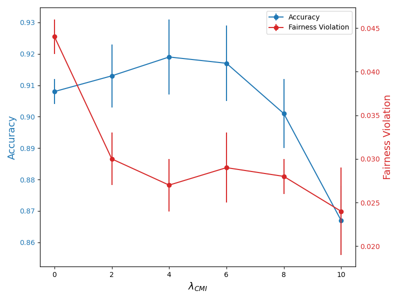
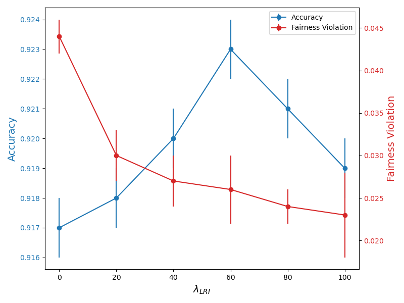
Figure 5: Top: Impact of varying $\lambda_{CMI}$ (with $\lambda_{LRI}$ fixed at 60) on classification accuracy and fairness violation (EOD) in the CelebA dataset classification task. Bottom: Impact of varying $\lambda_{LRI}$ (with $\lambda_{CMI}$ fixed at 5) on the same performance metrics.

9.4 Fair Classification

The objective of fair classification is to achieve a balance between minimizing fairness violations and maintaining high predictive performance. To evaluate the effectiveness of our proposed method, we conduct experiments on a diverse set of benchmark fairness datasets. For facial attribute classification tasks, we utilize the CelebA [29] and UTKFace [49] datasets. Following prior works [44, 47, 48, 15], we set the CelebA classification task to predict the ”Smiling” attribute, while for UTKFace, the objective is to classify whether a person depicted in the image is over 35 years old, with gender serving as the sensitive attribute. Additionally, the Dogs and Cats dataset [37] is used to distinguish between dogs and cats, with fur color as the sensitive attribute. Furthermore, we assess fair classification performance using the Colored MNIST dataset [18, 17, 35], which incorporates a controlled color bias in the standard MNIST dataset to simulate spurious correlations. In this dataset, a fixed color is assigned to each digit for a majority of the training samples—specifically, 70% of the samples have each of the 10 digits correlated with one of 10 predefined colors (with a small random perturbation), while the remaining 30% are assigned colors uniformly among the other options. For the test set, every digit is paired with a uniformly distributed color assignment to eliminate bias. In our fair classification task, the digit serves as the target attribute and the color as the sensitive attribute. Originally introduced to measure the color bias of classifiers predicting digits, this setup is critical for evaluating a model’s ability to disentangle the target digit information from the spurious color cues.

For model evaluation, we employ a 3-layered Multi-Layer Perceptron (MLP) classifier for all compared methods in all datasets. The input to the classifier consists of target-related features extracted from the pre-trained disentangled representations produced by each method. Specifically, we use $z_{Y}$ of our method to feed into the classifier, while using $z_{X}$ from FFVAE [6] and $z_{Y}$ from FADES [15]. For invariant learning methods including FairFactorVAE [19], FairDisCo [27], GVAE [7], the entire latent space is utilized for downstream classification tasks. For non-adversarial learning method, we use $z_{T}$ from ODVAE [42]. This experiment setup represents different disentanglement learning strategies as detailed in the related works section. To assess fairness violations, we use standard metrics including Demographic Parity (DP) [2] and Equalized Odds (EOD) [10]. Each method is evaluated over five experimental runs with different random dataset splits when the split is not predefined. This ensures robustness and statistical reliability in performance comparisons.

Demographic Parity (DP) is defined as:

$$DP=\left|\mathbb{P}(\hat{Y}=1\mid A=0)-\mathbb{P}(\hat{Y}=1\mid A=1)\right|,$$ (59)

where $\hat{Y}$ denotes the predicted outcome and $A$ represents the binary sensitive attribute (e.g., gender, race). This metric captures the absolute difference in positive prediction rates across the groups.

Equalized Odds (EOD) requires that the predictor’s true positive rates and false positive rates be equal across groups. It is defined as:

$$EOD\!=\!$$ (60)

$$\max_{y\in\{0,1\}}\!\left|\mathbb{P}(\hat{Y}\!=\!1\!\mid\!Y\!=\!y,A\!=\!0)\!-\!\mathbb{P}(\hat{Y}\!=\!1\!\mid\!Y\!=\!y,A\!=\!1)\right|,$$

where $Y$ represents the true outcome. This metric considers the maximum discrepancy over both outcome classes, ensuring fairness in both detection and error rates.

9.5 Fair Counterfactual Generation

To quantitatively assess the quality of the generated counterfactuals, we compare evaluation metrics between the direct reconstruction of the input image and the reconstructions obtained by randomly permuting the latent representations $z_{Y}$ and $z_{S}$ within the evaluation set. Specifically, we use the Fréchet Inception Distance (FID) [12, 15] to assess reconstruction fidelity and the Inception Score (IS) [5] to evaluate semantic and perceptual quality. Lower values of $\Delta\text{FID}$ indicate minimal distortion and higher translation quality, while lower values of $\Delta\text{IS}$ suggest that semantic and perceptual attributes are well preserved.

We first evaluate reconstruction fidelity by computing the FID between the original image set $X$ and its reconstructed counterpart $\hat{X}_{perm}$, where the reconstruction is performed after a random permutation of the latent codes. Formally, we define

$$\Delta\text{FID}=\text{FID}(X,\hat{X}_{perm}),$$ (61)

where $X=\{x_{i}\}_{i=1}^{N}$ denotes the set of original input images and $\hat{X}_{perm}=\{\hat{x}_{i}^{perm}\}_{i=1}^{N}$ represents the corresponding reconstructed images. A lower $\Delta\text{FID}$ value implies higher translation quality, as it reflects minimal image distortion and fidelity loss during the counterfactual generation process.

In addition, we assess the semantic and perceptual quality by employing the Inception Score. The IS for the direct reconstruction is computed as

$$\text{IS}(X)=\exp\left(\mathbb{E}_{x\sim p(x)}\left[\text{KL}\left(p(y|x)\,\|\,p(y)\right)\right]\right),$$ (62)

where $p(y|x)$ denotes the conditional probability distribution over labels given an image $x$, and $p(y)$ represents the marginal distribution over labels. Similarly, we compute $\text{IS}(\hat{X}_{perm})$ for the permuted reconstructions. The absolute difference between these scores is then defined as

$$\Delta\text{IS}=\left|\text{IS}(X)-\text{IS}(\hat{X}_{perm})\right|.$$ (63)

A lower $\Delta\text{IS}$ value indicates that the semantic and perceptual attributes of the image are well-preserved after translation, thereby validating the quality of the counterfactuals generated.

Together, these complementary metrics provide a comprehensive evaluation of the counterfactual generation quality. By quantifying both fidelity and semantic consistency, our experimental design rigorously validates the performance of the proposed method.

9.6 Fair Fine-Grained Image Editing

Similarly, we quantitatively assess the quality of fine-grained image editing by computing the differences in evaluation metrics between the direct reconstruction of the input image and the reconstructions obtained via latent code traversals with varying $\lambda$ combinations. Specifically, we define

$$\Delta\text{FID}=\text{FID}(X,\hat{X}_{trav}),$$ (64)

and

$$\Delta\text{IS}=\left|\text{IS}(X)-\text{IS}(\hat{X}_{trav})\right|,$$ (65)

where $X=\{x_{i}\}_{i=1}^{N}$ denotes the set of original input images, and $\hat{X}_{trav}=\{\hat{x}_{i}^{trav}\}_{i=1}^{N}$ represents the corresponding reconstructed images obtained via latent code traversals.

In our experimental setup, where Smiling is the target attribute $Y$ and Gender is the sensitive attribute $S$, we generate interpolated latent codes between source and reference images. Specifically, the interpolation is performed on the latent codes $z_{Y}$, $z_{S}$, and $z_{R}$. The interpolation parameters for $z_{Y}$ and $z_{S}$ are set to

$$\lambda\in\{0,\,0.33,\,0.66,\,1\},$$

while for $z_{R}$ the parameters are chosen from

$$\lambda\in\{0,\,0.5,\,1\}.$$

Thus, the overall combination of latent modifications involves $4\times 4\times 3$ distinct $\lambda$ combinations, corresponding to different configurations for $z_{Y}$, $z_{S}$, and $z_{R}$. During each traversal, the latent code $z_{X}$ remains unchanged, ensuring that the variations reflect only the task-relevant attribute transformations.

In this context, $\Delta\text{FID}$ measures the reconstruction fidelity, with lower values indicating that the traversed reconstructions closely resemble the original images in terms of their distribution. Likewise, $\Delta\text{IS}$ quantifies the preservation of semantic and perceptual quality; lower values suggest that the intrinsic content and visual features remain consistent despite the latent manipulations.

10 Additional Experiment

10.1 Fair Classification

Table 5: Evaluation of downstream classification tasks on CelebA dataset for various target attributes from learned representation. Best in bold, second in red.

                 CelebA Classification Performance Methods Smiling Blond Hair Attractive Young Acc $\uparrow$ EOD $\downarrow$ DP $\downarrow$ Acc $\uparrow$ EOD $\downarrow$ DP $\downarrow$ Acc $\uparrow$ EOD $\downarrow$ DP $\downarrow$ Acc $\uparrow$ EOD $\downarrow$ DP $\downarrow$   FADES [15] [CVPR’24] 0.918 0.034 0.135 0.930 0.118 0.153 0.763 0.308 0.346 0.835 0.164 0.169 GVAE [7] [CVPR’20] 0.919 0.047 0.131 0.940 0.484 0.247 0.779 0.564 0.431 0.841 0.209 0.176 FFVAE [6] [PMLR’19] 0.892 0.076 0.072 0.926 0.301 0.201 0.749 0.359 0.310 0.832 0.281 0.195 ODVAE [42] [ECCV’20] 0.886 0.039 0.103 0.896 0.465 0.210 0.719 0.551 0.438 0.827 0.297 0.262 FairDisCo [27] [KDD’22] 0.839 0.074 0.051 0.916 0.465 0.234 0.750 0.515 0.411 0.839 0.226 0.196 FairFactorVAE [28] 0.914 0.055 0.136 0.918 0.326 0.174 0.709 0.459 0.350 0.827 0.296 0.318 CAD-VAE (Ours) 0.923 0.021 0.112 0.939 0.105 0.137 0.773 0.268 0.290 0.847 0.151 0.155  

To further validate the efficacy of our method in achieving fairness via effective disentanglement, we conducted additional experiments with different target attributes. Following the experimental setup in the main paper on the CelebA dataset, our evaluations extended beyond the ”Smiling” attribute to include other widely adopted target labels, such as ”Blond Hair”, ”Attractiveness” and ”Young” under gender bias conditions. As summarized in Table 5, our method consistently achieves competitive accuracy while significantly mitigating fairness violations compared to existing approaches. These results further substantiate the robustness of our fair disentanglement learning strategy and demonstrate its applicability across a variety of target attributes.

10.2 Fair Counterfactual Generation

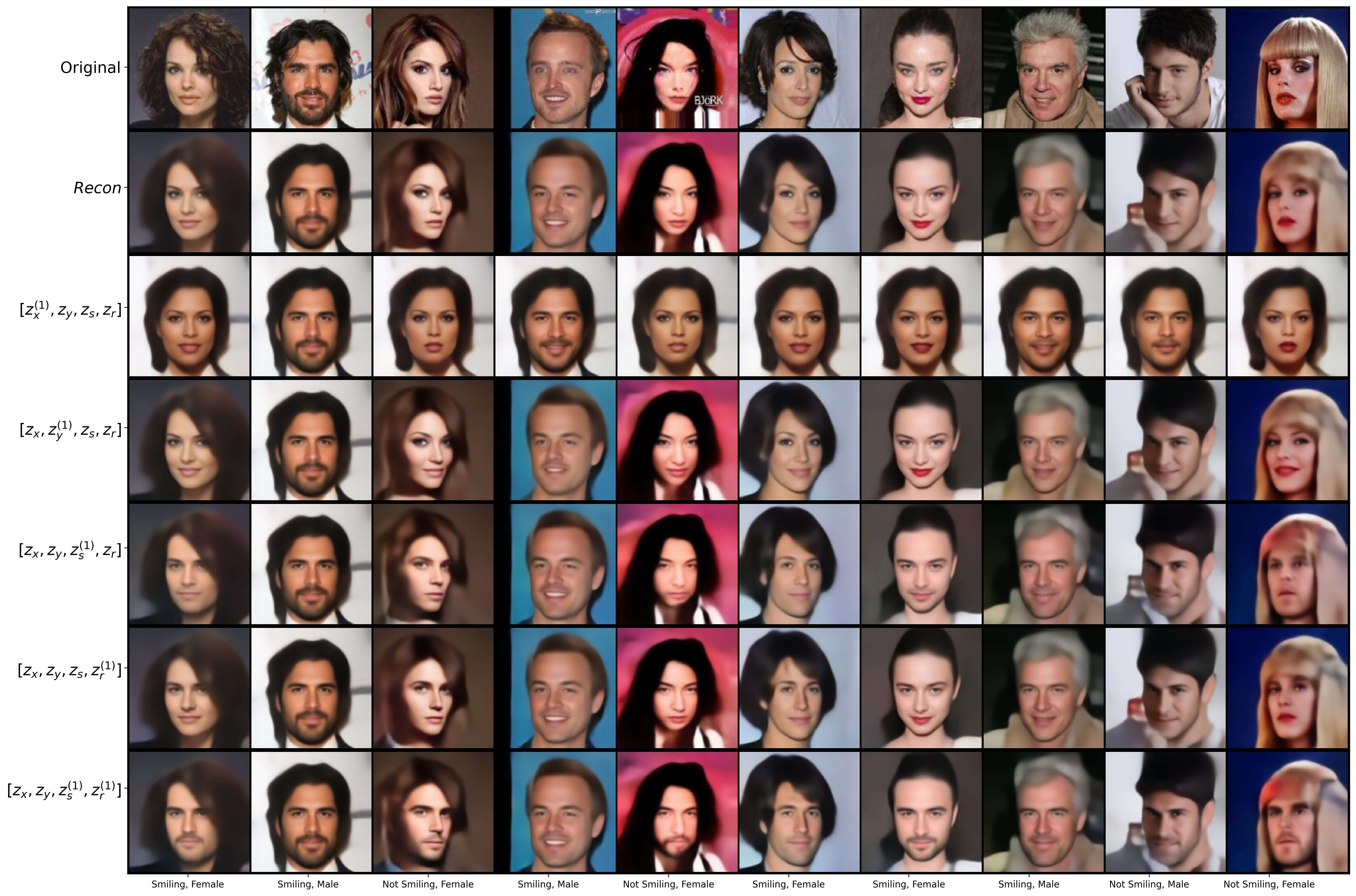
Figure 10: Examples of Fair Counterfactual Generation. The image in the 1th column serves as the reference, while the images in the remaining columns are the source images.

In this subsection, we present the results of counterfactual generation on the CelebA dataset[29]. Figure 9 and Figure 10 display a grid of images, each row corresponding to a specific configuration of latent codes. The second row shows the direct reconstruction of the original input image, which is shown in the first row. The intermediate rows illustrate variations derived from different latent code substitutions. For instance, in the third row of Figure 9, the latent code configuration $[z_{X}^{(0)},z_{Y},z_{S},z_{R}]$ is used, where the digit 0 indicates that the reference image is the one in the 0th column. In this configuration, the images in the subsequent columns are generated by replacing their latent code $z_{X}$ with the $z_{X}$ from the 0th column image, while the remaining latent codes ($z_{Y}$, $z_{S}$, and $z_{R}$) are retained. This approach effectively alters the corresponding features in the generated images. Our experiments demonstrate that both sensitive and target attributes can be distinctly translated. Moreover, the method supports the simultaneous translation of these attributes, thereby providing greater flexibility in generating counterfactuals. For instance, given an image of a smiling female, our approach can produce images representing a non-smiling male, a non-smiling female, and a smiling male, contributing to improved individual fairness [16] by ensuring that individuals with similar characteristics but different sensitive attributes receive comparable outcomes.

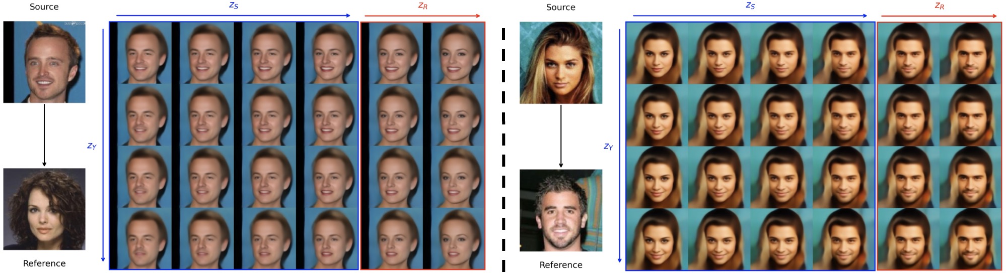
Figure 6: Examples of Fair Fine-Grained Image Editing. The leftmost column shows the source and reference images. The blue-framed section displays images generated by interpolating $z_{Y}$ and $z_{S}$ (with $z_{R}$ and $z_{X}$ fixed), where the horizontal axis varies $z_{S}$ and the vertical axis varies $z_{Y}$. The red-framed section illustrates images produced by interpolating $z_{Y}$ and $z_{R}$ (with $z_{S}$ fully replaced by the reference and $z_{X}$ constant). Modification in one latent code minimally affecting others, harness $z_{R}$ to edit sensitive relevant feature(makeup or mustache).

10.3 Fair Fine-Grained Image Editing

In this subsection, we display more fair fine-grained image editing results in Figure 6, following the experiment setup in the main paper. Specifically, as the correlated latent code $z_{R}$ captures sensitive relevant information, we can explicitly control these properties: in the left subfigure, we gradually introduce makeup (such as enhanced lipstick and eyeshadow), while in the right subfigure, we progressively add a mustache.

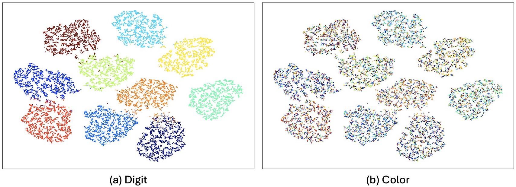
(a) CAD-VAE

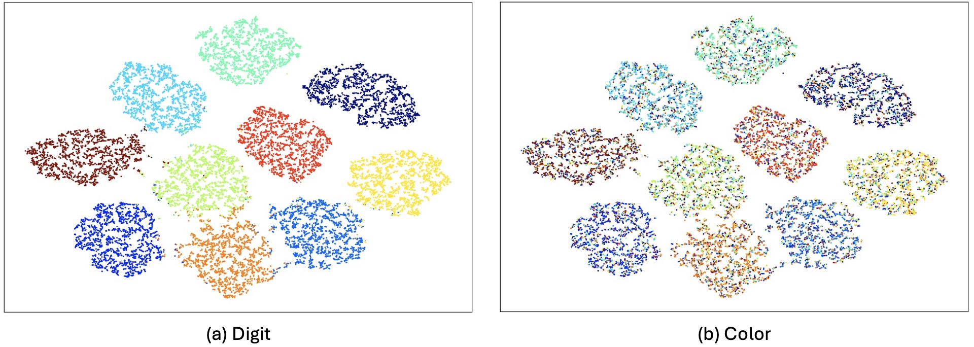
(b) FADES [15]

(c) GVAE [7]

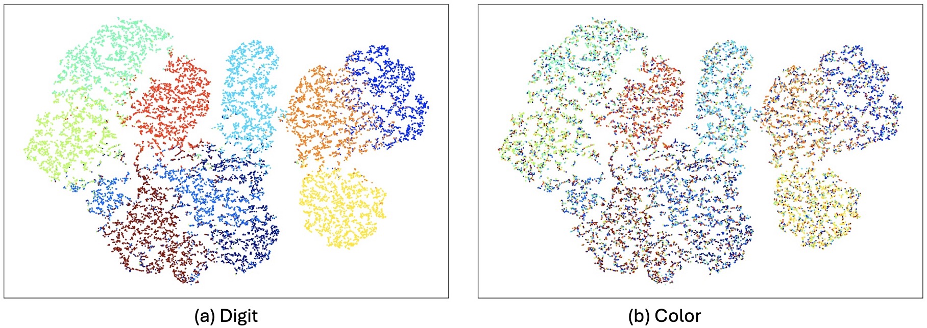
(d) FFVAE [6]

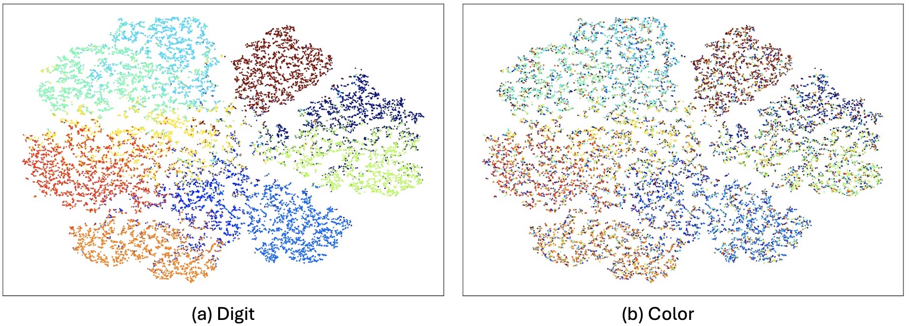
(e) ODVAE [42]

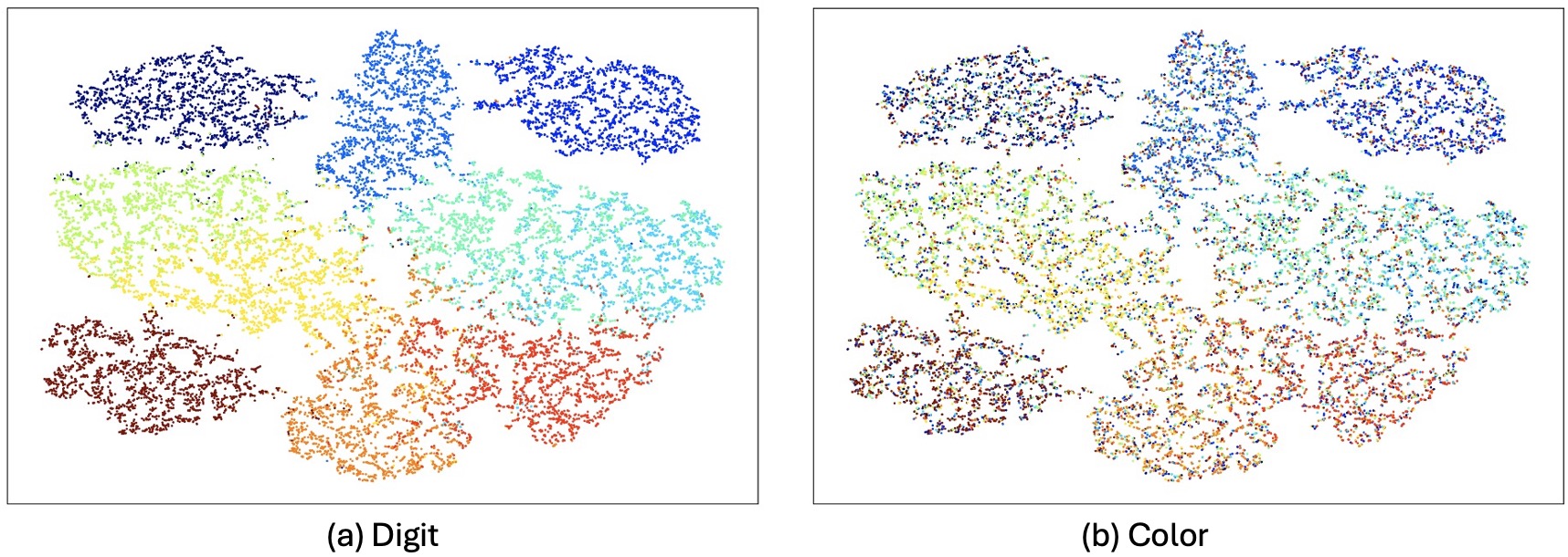
(f) FairDisCo [27]

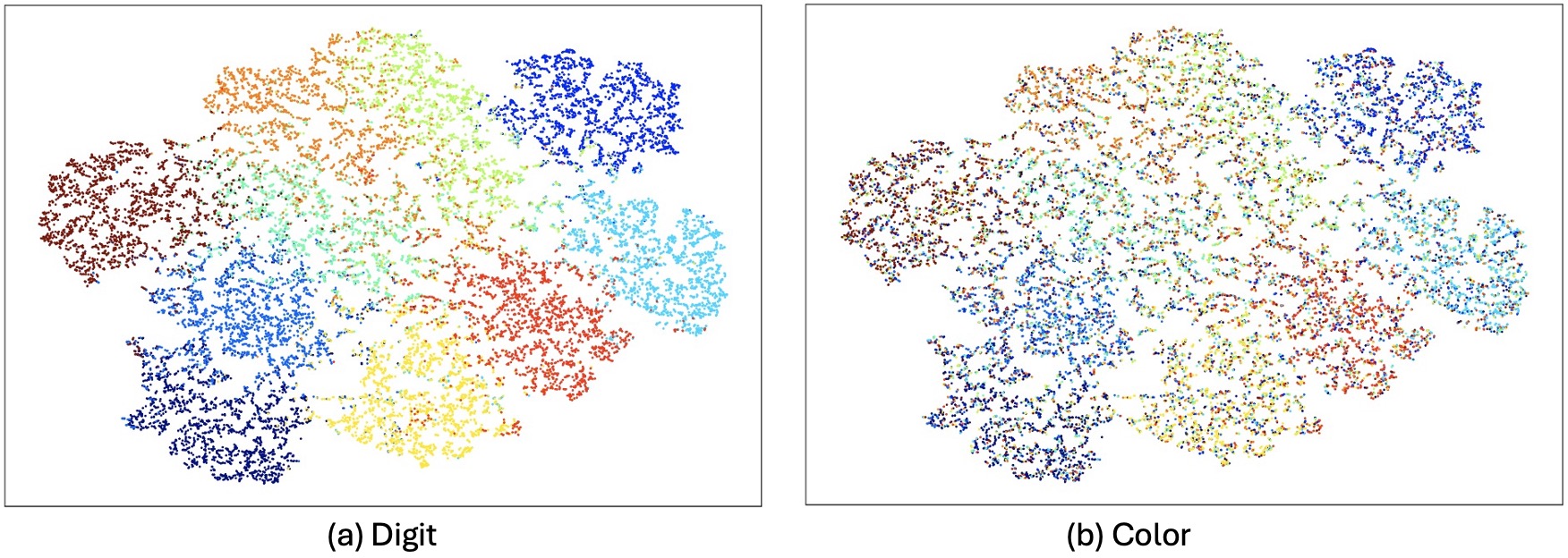
(g) FairFactorVAE [28]

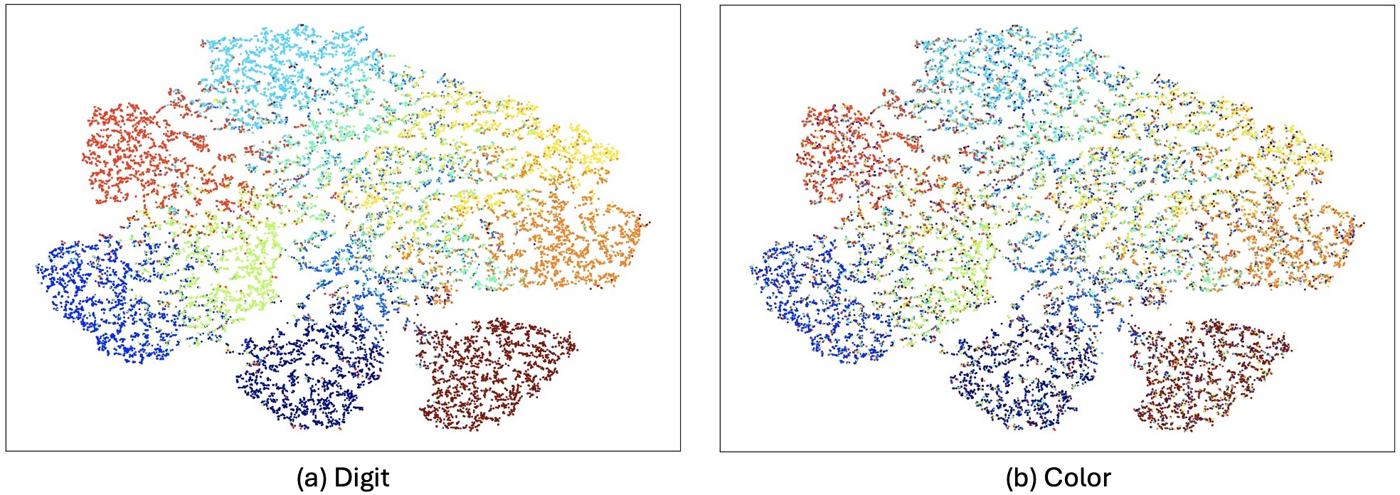
(h) FactorVAE [19]

Figure 7: t-SNE visualization of the target code from the test set for each method. Left subfigure is colored by Digit; right subfigure is colored by Color.

10.4 t-SNE Visualization

To better understand the distribution and disentanglement of the learned representation, we present a t-SNE visualization analysis of the target latent code of each method. The visualizations are derived from experiments in Section 4.1 of the main paper where the model is trained on a biased color MNIST dataset and tested on an unbiased color MNIST dataset. Each figure consists of two subfigures: the left subfigure is colored according to the Digit attribute (target attribute), and the right subfigure is colored according to the Color attribute (sensitive attribute). Clear and distinct clustering in the left subfigure indicates that the model has learned a robust and discriminative representation of the target attribute, thereby enhancing its recognizability. Conversely, if the right subfigure exhibits discernible color clusters, it suggests a correlation between the target and sensitive attributes, indicating weaker disentanglement performance. A uniform color distribution in the right subfigure, however, confirms that the sensitive information has been effectively filtered out.

This visualization in Figure 7 demonstrates that our proposed method effectively disentangles the learned representation. The target attribute (Digit) exhibits distinct, well-separated clusters with clear classification boundaries and a pure distribution, while the sensitive attribute (Color) is uniformly distributed and unrecognizable. This confirms that our method achieves superior separation of the target attribute without introducing unwanted bias from the sensitive attribute.

10.5 Text-to-Image Editing

To further validate the capability and explore the applicability of our method, we integrated it as an adaptor on top of a pre-trained, frozen CLIP image encoder [39] and trained it on datasets including CelebA [29] and Facet [9] to enhance fairness in vision-language tasks. Table 6 and Table 7 present the experimental results on CelebA and Facet, respectively. These results demonstrate that our approach significantly improves fairness without compromising performance compared to the linear probing baseline (ERM), underscoring its potential for a range of vision-language tasks such as search and image retrieval with fairness considerations.

In Table 7, we also present an ablation study that examines the contribution of each loss term, as detailed in the last three rows. Each row represents training using only $L_{ELBO}$, without $L_{CMI}$, and without $L_{LRI}$, respectively.

Table 6: Performance of CLIP(ViTB/32) on CelebA dataset.

  Method Acc $\uparrow$ EOD $\downarrow$ DP $\downarrow$   Zero-shot 0.857 0.834 0.715 Linear prob 0.918 0.924 0.837 CAD-VAE 0.921 0.037 0.133  

Table 7: Performance of CLIP(ViTB/32) on Facet dataset. WG: Worst Group, Gap: Difference between WG and Avg.

  Method Top-1 Acc. (%) Top-3 Acc. (%) WG $\uparrow$ Avg $\uparrow$ Gap $\downarrow$ WG $\uparrow$ Avg $\uparrow$ Gap $\downarrow$   Zero-shot 2.79 53.45 50.66 15.31 76.79 61.48 Linear prob 1.17 65.46 64.29 1.79 85.34 83.55 CAD-VAE 69.97 70.54 0.57 85.36 85.95 0.59 (Abl.) $\mathcal{L}_{\mathrm{ELBO}}$ 16.34 67.27 50.93 37.24 86.96 49.72 (Abl.) w/o $\mathcal{L}_{\mathrm{CMI}}$ 20.43 67.67 47.24 25.41 91.12 65.71 (Abl.) w/o $\mathcal{L}_{\mathrm{LRI}}$ 24.03 64.19 40.16 29.17 87.42 58.25  

Furthermore, we applied our method in StyleCLIP [38] as a fair discriminator to address inherent fairness issues, such as career-gender biases, which persist even when an identity preservation loss is employed. As illustrated in Figure 8, StyleCLIP [38] exhibits a bias by correlating the role of “dancer” with a specific gender. In contrast, our method effectively mitigates this bias while maintaining the efficacy of attribute modification.

(a) Original

(b) StyleCLIP

(c) StyleCLIP+

Figure 8: Style transfer using StyleCLIP and the CAD-VAE extension. This example transforms the (a) into “a dancer with long blonde hair.” “StyleCLIP+” means StyleCLIP + CAD-VAE.

Figure 9: Examples of Fair Counterfactual Generation. The image in the 0th column serves as the reference, while the images in the remaining columns are the source images.

11 Limitation and Future Works

The limitations of our work can be summarized in two main aspects. First, while our study addresses the inherent trade-off between fairness and performance under certain data biases, fairness violations can arise from a variety of sources. CAD-VAE specifically mitigates the unwanted correlation between sensitive attribute and target attribute, which represents one primary cause of fairness issues. However, in real-world applications, additional factors such as under-representation, intrinsic model bias, and the presence of missing or noisy features often co-occur, exacerbating fairness violations. Future research should aim to extend our theoretical framework to encompass these diverse and often overlapping sources of bias. Second, our current approach requires the availability of both target and sensitive attribute information during training. In many practical scenarios, acquiring such labeled data can be challenging due to high annotation costs or legal and regulatory restrictions. A promising direction for future work is to develop methods that relax this dependency, potentially through unsupervised or semi-supervised techniques, to learn fair and disentangled representations without explicit reliance on labeled sensitive information.

References

- Bai et al. [2024] Jinbin Bai, Tian Ye, Wei Chow, Enxin Song, Qing-Guo Chen, Xiangtai Li, Zhen Dong, Lei Zhu, and YAN Shuicheng. Meissonic: Revitalizing masked generative transformers for efficient high-resolution text-to-image synthesis. In The Thirteenth International Conference on Learning Representations, 2024.
- Barocas and Selbst [2016] Solon Barocas and Andrew D Selbst. Big data’s disparate impact. Calif. L. Rev., 104:671, 2016.
- Chen et al. [2018] Ricky TQ Chen, Xuechen Li, Roger B Grosse, and David K Duvenaud. Isolating sources of disentanglement in variational autoencoders. Advances in neural information processing systems, 31, 2018.
- Chiappa [2019] Silvia Chiappa. Path-specific counterfactual fairness. In Proceedings of the AAAI conference on artificial intelligence, pages 7801–7808, 2019.
- Chong and Forsyth [2020] Min Jin Chong and David Forsyth. Effectively unbiased fid and inception score and where to find them. In Proceedings of the IEEE/CVF conference on computer vision and pattern recognition, pages 6070–6079, 2020.
- Creager et al. [2019] Elliot Creager, David Madras, Jörn-Henrik Jacobsen, Marissa Weis, Kevin Swersky, Toniann Pitassi, and Richard Zemel. Flexibly fair representation learning by disentanglement. In International conference on machine learning, pages 1436–1445. PMLR, 2019.
- Ding et al. [2020] Zheng Ding, Yifan Xu, Weijian Xu, Gaurav Parmar, Yang Yang, Max Welling, and Zhuowen Tu. Guided variational autoencoder for disentanglement learning. In Proceedings of the IEEE/CVF conference on computer vision and pattern recognition, pages 7920–7929, 2020.
- Dressel and Farid [2018] Julia Dressel and Hany Farid. The accuracy, fairness, and limits of predicting recidivism. Science Advances, 4(1):eaao5580, 2018.
- Gustafson et al. [2023] Laura Gustafson, Chloe Rolland, Nikhila Ravi, Quentin Duval, Aaron Adcock, Cheng-Yang Fu, Melissa Hall, and Candace Ross. Facet: Fairness in computer vision evaluation benchmark, 2023.
- Hardt et al. [2016] Moritz Hardt, Eric Price, and Nati Srebro. Equality of opportunity in supervised learning. Advances in neural information processing systems, 29, 2016.
- He et al. [2016] Kaiming He, Xiangyu Zhang, Shaoqing Ren, and Jian Sun. Deep residual learning for image recognition. In Proceedings of the IEEE conference on computer vision and pattern recognition, pages 770–778, 2016.
- Heusel et al. [2017] Martin Heusel, Hubert Ramsauer, Thomas Unterthiner, Bernhard Nessler, and Sepp Hochreiter. Gans trained by a two time-scale update rule converge to a local nash equilibrium. Advances in neural information processing systems, 30, 2017.
- Higgins et al. [2017] Irina Higgins, Loic Matthey, Arka Pal, Christopher Burgess, Xavier Glorot, Matthew Botvinick, Shakir Mohamed, and Alexander Lerchner. beta-vae: Learning basic visual concepts with a constrained variational framework. In International conference on learning representations, 2017.
- Hwa et al. [2024] Jensen Hwa, Qingyu Zhao, Aditya Lahiri, Adnan Masood, Babak Salimi, and Ehsan Adeli. Enforcing conditional independence for fair representation learning and causal image generation. In Proceedings of the IEEE/CVF Conference on Computer Vision and Pattern Recognition, pages 103–112, 2024.
- Jang and Wang [2024] Taeuk Jang and Xiaoqian Wang. Fades: Fair disentanglement with sensitive relevance. In Proceedings of the IEEE/CVF Conference on Computer Vision and Pattern Recognition (CVPR), pages 12067–12076, 2024.
- Jung et al. [2025] Sangwon Jung, Sumin Yu, Sanghyuk Chun, and Taesup Moon. Do counterfactually fair image classifiers satisfy group fairness?–a theoretical and empirical study. Advances in Neural Information Processing Systems, 37:56041–56053, 2025.
- Kim et al. [2019] Byungju Kim, Hyunwoo Kim, Kyungsu Kim, Sungjin Kim, and Junmo Kim. Learning not to learn: Training deep neural networks with biased data. In Proceedings of the IEEE/CVF Conference on Computer Vision and Pattern Recognition (CVPR), 2019.
- Kim et al. [2021a] Eungyeup Kim, Jihyeon Lee, and Jaegul Choo. Biaswap: Removing dataset bias with bias-tailored swapping augmentation. In Proceedings of the IEEE/CVF International Conference on Computer Vision, pages 14992–15001, 2021a.
- Kim and Mnih [2018] Hyunjik Kim and Andriy Mnih. Disentangling by factorising. In International conference on machine learning, pages 2649–2658. PMLR, 2018.
- Kim et al. [2021b] Hyemi Kim, Seungjae Shin, JoonHo Jang, Kyungwoo Song, Weonyoung Joo, Wanmo Kang, and Il-Chul Moon. Counterfactual fairness with disentangled causal effect variational autoencoder. In Proceedings of the AAAI Conference on Artificial Intelligence, pages 8128–8136, 2021b.
- Kingma and Welling [2022] Diederik P Kingma and Max Welling. Auto-encoding variational bayes, 2022.
- Kohavi [1996] Ron Kohavi. Scaling up the accuracy of naive-bayes classifiers: a decision-tree hybrid. In Proceedings of the Second International Conference on Knowledge Discovery and Data Mining, page 202–207. AAAI Press, 1996.
- Kusner et al. [2017] Matt J Kusner, Joshua Loftus, Chris Russell, and Ricardo Silva. Counterfactual fairness. Advances in neural information processing systems, 30, 2017.
- Lahoti et al. [2020] Preethi Lahoti, Alex Beutel, Jilin Chen, Kang Lee, Flavien Prost, Nithum Thain, Xuezhi Wang, and Ed H. Chi. Fairness without demographics through adversarially reweighted learning, 2020.
- Li et al. [2025] Haoxuan Li, Yue Liu, Zhi Geng, and Kun Zhang. A local method for satisfying interventional fairness with partially known causal graphs. Advances in Neural Information Processing Systems, 37:135415–135436, 2025.
- Liu et al. [2021] Evan Zheran Liu, Behzad Haghgoo, Annie S. Chen, Aditi Raghunathan, Pang Wei Koh, Shiori Sagawa, Percy Liang, and Chelsea Finn. Just train twice: Improving group robustness without training group information, 2021.
- Liu et al. [2022] Ji Liu, Zenan Li, Yuan Yao, Feng Xu, Xiaoxing Ma, Miao Xu, and Hanghang Tong. Fair representation learning: An alternative to mutual information. In Proceedings of the 28th ACM SIGKDD Conference on Knowledge Discovery and Data Mining, pages 1088–1097, 2022.
- Liu et al. [2023] Shaofan Liu, Shiliang Sun, and Jing Zhao. Fair transfer learning with factor variational auto-encoder. Neural Processing Letters, 55(3):2049–2061, 2023.
- Liu et al. [2015] Ziwei Liu, Ping Luo, Xiaogang Wang, and Xiaoou Tang. Deep learning face attributes in the wild. In Proceedings of the IEEE international conference on computer vision, pages 3730–3738, 2015.
- Madras et al. [2018] David Madras, Elliot Creager, Toniann Pitassi, and Richard Zemel. Learning adversarially fair and transferable representations. In International Conference on Machine Learning, pages 3384–3393. PMLR, 2018.
- Mathieu et al. [2019] Emile Mathieu, Tom Rainforth, N. Siddharth, and Yee Whye Teh. Disentangling disentanglement in variational autoencoders, 2019.
- Mehrabi et al. [2021] Ninareh Mehrabi, Fred Morstatter, Nripsuta Saxena, Kristina Lerman, and Aram Galstyan. A survey on bias and fairness in machine learning. ACM computing surveys (CSUR), 54(6):1–35, 2021.
- Meo et al. [2024] Cristian Meo, Louis Mahon, Anirudh Goyal, and Justin Dauwels. $\alpha$TC-VAE: On the relationship between disentanglement and diversity. In The Twelfth International Conference on Learning Representations, 2024.
- Montanaro et al. [2024] Antonio Montanaro, Luca Savant Aira, Emanuele Aiello, Diego Valsesia, and Enrico Magli. Motioncraft: Physics-based zero-shot video generation. In Advances in Neural Information Processing Systems 38: Annual Conference on Neural Information Processing Systems 2024, NeurIPS 2024, Vancouver, BC, Canada, December 10 - 15, 2024, 2024.
- Nam et al. [2020] Junhyun Nam, Hyuntak Cha, Sungsoo Ahn, Jaeho Lee, and Jinwoo Shin. Learning from failure: De-biasing classifier from biased classifier. Advances in Neural Information Processing Systems, 33:20673–20684, 2020.
- Park et al. [2020] Sungho Park, Dohyung Kim, Sunhee Hwang, and Hyeran Byun. Readme: Representation learning by fairness-aware disentangling method, 2020.
- Parkhi et al. [2012] Omkar M Parkhi, Andrea Vedaldi, Andrew Zisserman, and CV Jawahar. Cats and dogs. In 2012 IEEE conference on computer vision and pattern recognition, pages 3498–3505. IEEE, 2012.
- Patashnik et al. [2021] Or Patashnik, Zongze Wu, Eli Shechtman, Daniel Cohen-Or, and Dani Lischinski. Styleclip: Text-driven manipulation of stylegan imagery. In Proceedings of the IEEE/CVF International Conference on Computer Vision (ICCV), pages 2085–2094, 2021.
- Radford et al. [2021] Alec Radford, Jong Wook Kim, Chris Hallacy, Aditya Ramesh, Gabriel Goh, Sandhini Agarwal, Girish Sastry, Amanda Askell, Pamela Mishkin, Jack Clark, Gretchen Krueger, and Ilya Sutskever. Learning transferable visual models from natural language supervision, 2021.
- Roy and Boddeti [2019] Proteek Chandan Roy and Vishnu Naresh Boddeti. Mitigating information leakage in image representations: A maximum entropy approach, 2019.
- Sánchez-Martin et al. [2022] Pablo Sánchez-Martin, Miriam Rateike, and Isabel Valera. Vaca: Designing variational graph autoencoders for causal queries. In Proceedings of the AAAI Conference on Artificial Intelligence, pages 8159–8168, 2022.
- Sarhan et al. [2020] Mhd Hasan Sarhan, Nassir Navab, Abouzar Eslami, and Shadi Albarqouni. Fairness by learning orthogonal disentangled representations. In Computer Vision–ECCV 2020: 16th European Conference, Glasgow, UK, August 23–28, 2020, Proceedings, Part XXIX 16, pages 746–761. Springer, 2020.
- Wang et al. [2024] Xin Wang, Hong Chen, Si’ao Tang, Zihao Wu, and Wenwu Zhu. Disentangled representation learning. IEEE Transactions on Pattern Analysis and Machine Intelligence, 46(12):9677–9696, 2024.
- Wang et al. [2022] Zhibo Wang, Xiaowei Dong, Henry Xue, Zhifei Zhang, Weifeng Chiu, Tao Wei, and Kui Ren. Fairness-aware adversarial perturbation towards bias mitigation for deployed deep models. In Proceedings of the IEEE/CVF conference on computer vision and pattern recognition, pages 10379–10388, 2022.
- Wu et al. [2019] Yongkai Wu, Lu Zhang, and Xintao Wu. Counterfactual fairness: Unidentification, bound and algorithm. In Proceedings of the twenty-eighth international joint conference on Artificial Intelligence, 2019.
- Xu et al. [2018] Depeng Xu, Shuhan Yuan, Lu Zhang, and Xintao Wu. Fairgan: Fairness-aware generative adversarial networks. In 2018 IEEE international conference on big data (big data), pages 570–575. IEEE, 2018.
- Xu et al. [2020] Tian Xu, Jennifer White, Sinan Kalkan, and Hatice Gunes. Investigating bias and fairness in facial expression recognition. In Computer Vision–ECCV 2020 Workshops: Glasgow, UK, August 23–28, 2020, Proceedings, Part VI 16, pages 506–523. Springer, 2020.
- Zeng et al. [2022] Huimin Zeng, Zhenrui Yue, Lanyu Shang, Yang Zhang, and Dong Wang. Boosting demographic fairness of face attribute classifiers via latent adversarial representations. In 2022 IEEE International Conference on Big Data (Big Data), pages 1588–1593. IEEE, 2022.
- Zhang et al. [2017] Zhifei Zhang, Yang Song, and Hairong Qi. Age progression/regression by conditional adversarial autoencoder. In Proceedings of the IEEE conference on computer vision and pattern recognition, pages 5810–5818, 2017.
- Zhou et al. [2024] Zeyu Zhou, Tianci Liu, Ruqi Bai, Jing Gao, Murat Kocaoglu, and David I Inouye. Counterfactual fairness by combining factual and counterfactual predictions. arXiv preprint arXiv:2409.01977, 2024.
- Zhu et al. [2023] Huaisheng Zhu, Enyan Dai, Hui Liu, and Suhang Wang. Learning fair models without sensitive attributes: A generative approach. Neurocomputing, 561:126841, 2023.