Variation of Dense Gas Mass-Luminosity conversion factor with metallicity in the Milky Way

Abstract

HCN and HCO⁺ are the most common dense gas tracers used both in the Milky Way and external galaxies. The luminosity of HCN and HCO⁺ $J=1\rightarrow 0$ lines are converted to a dense gas mass by the conversion factor, $\alpha_{Q}$. Traditionally, this $\alpha_{Q}$ has been considered constant throughout the Galaxy and in other galaxies, regardless of the environment. We analyzed 17 outer Galaxy clouds and 5 inner Galaxy clouds with metallicities ranging from 0.38 Z_⊙ to 1.29 Z_⊙. Our analysis indicates that $\alpha_{Q}$ is not constant; instead, it varies with metallicity. The metallicity-corrected $\alpha_{Q}$ derived from the HCN luminosity of the entire cloud is almost three times higher in the outer Galaxy than in the inner galaxy. In contrast, HCO⁺ seems less sensitive to metallicity. We recommend using the metallicity-corrected dense gas conversion factors $\alpha^{{}^{\prime}}_{\rm tot,Gas}(\rm HCN)=19.5^{+5.6}_{-4.4}Z^{(-1.53\pm 0.59)}$ and $\alpha^{{}^{\prime}}_{\rm tot,Gas}(\rm HCO^{+})=21.4^{+5.5}_{-4.4}Z^{(-1.32\pm 0.55)}$ for extragalactic studies. Radiation from nearby stars has an effect on the conversion factor of similar magnitude as that of the metallicity. If we extend the metallicity-corrected scaling relation for HCN to the Central Molecular Zone, the value of $\alpha(\mbox{{\rm HCN}})$ becomes $1/3$ to $1/2$ of the local values. This effect could partially account for the low star formation rate per dense gas mass observed in the CMZ.

1 Introduction

Studies of molecular clouds within the Milky Way found that most of the dense cores and young stellar objects (YSOs) are associated with regions of high surface density, measured by visual extinction, $\mbox{$A_{\rm V}$}>8\ \mathrm{mag}$ (Heiderman et al., 2010; Lada et al., 2010, 2012). Also, Vutisalchavakul et al. (2016) found a nearly linear relationship between the star formation rate (SFR) and the mass of dense gas, as determined by millimeter continuum emission data from the Bolocam Galactic Plane Survey (BGPS, Ginsburg et al. 2013), particularly for distant and massive clouds. Some studies have indicated a decreased star formation efficiency for the most massive dense clumps (Wells et al., 2022), but Mattern et al. (2024) found that the star formation efficiency in dense gas is nearly constant. Their analysis of all southern molecular clouds within 3 kpc shows that the amount of dense gas is the primary indicator of the star formation rate. On extragalactic scales, a pioneering study by Gao & Solomon (2004a) identified a robust linear relationship between far-infrared luminosities, related to the SFR, and HCN line luminosities, which serve as measures of dense gas content. A consistent observation has emerged from several studies investigating entire galaxies (Gao & Solomon, 2004a; Zhang et al., 2014; Liu et al., 2015) and spatially resolved nearby galaxies (Chen et al., 2015; Tan et al., 2018; Jiménez-Donaire et al., 2019; Heyer et al., 2022; Neumann et al., 2023), utilizing various dense gas tracers such as HCN, HCO⁺, CS, and high-$J$ ¹²CO lines. These studies suggest that the denser parts of the molecular clouds serve as the direct sources of fuel for the process of star formation. The correlation between star formation rate (SFR) and the luminosity of HCN $J=1\rightarrow 0$ emission ($L({\rm HCN})$) is tighter than the correlation of SFR with ¹²CO $J=1\rightarrow 0$ emission, supporting the idea that dense parts of molecular clouds are more likely sites of star formation.

There are three distinct methods in use to measure the mass of gas associated with star formation: a surface density criterion ($\mbox{$A_{\rm V}$}>8\ \mathrm{mag}$) used in nearby clouds (Heiderman et al., 2010; Lada et al., 2010, 2012), a millimeter continuum emission method used in more distant clouds in our Galaxy (Vutisalchavakul et al., 2016; Urquhart et al., 2024), and a line luminosity method (usually HCN, but also HCO⁺) (Wu et al., 2005; Evans et al., 2020; Patra et al., 2022) used most often in other galaxies. While the first method is based on column density, the last two methods are more sensitive to volume density because of the limited spatial scales available to ground-based millimeter continuum observations or the excitation criterion for molecules with large dipole moments (Shirley, 2015). Millimeter continuum dust emission is an optically thin tracer of gas column density in dense molecular clouds, effectively identifying molecular clumps where star formation may occur. However, due to the methods used to remove atmospheric fluctuations, the BGPS emission traces volume density, with the characteristic density probed decreasing with distance, averaging between $5\times 10^{3}$ to $1\times 10^{4}$ $\rm cm^{-3}$ for distances of 2-6 kpc (Dunham et al., 2011). We will compare these three methods in this paper.

Clouds in our Galaxy provide opportunities to study in greater detail the relation of these dense gas tracers to the mass of dense gas. Wu et al. (2005) showed that the relation between star formation rate and the luminosity of HCN seen in other galaxies persists into dense cores in Galactic clouds. However, subsequent studies that mapped HCN emission over larger regions found that a very substantial fraction of $L({\rm HCN})$ arises in lower density parts of the cloud (Shimajiri et al., 2017; Kauffmann et al., 2017; Pety et al., 2017; Evans et al., 2020; Barnes et al., 2020; Patra et al., 2022). In part, the ability of relatively diffuse parts of the cloud to produce significant contributions to $L({\rm HCN})$  arises from the good sensitivity of newer receivers and the fact that the area and mass of molecular clouds is dominated by low-density gas. Trapping of photons in optically thick lines and other excitation effects allows gas at densities far below the so-called critical density to produce detectable emission (Evans et al., 2020; Patra et al., 2022; Shirley, 2015). In addition, photo-ionization by ultraviolet photons can cause electron collisions to contribute to the excitation of HCN (Goldsmith & Kauffmann, 2017). Taken together, these results indicate that the relationship between $L({\rm HCN})$ and the mass of dense gas is more complicated than usually assumed.

A complication that has not been explored so far is the likelihood that the HCN abundance and hence emission will be affected by metallicity. It has become increasingly recognized that the mass-luminosity conversion factor for ¹²CO is not constant, but varies with metallicity (Gong et al., 2020; Hu et al., 2022). In extragalactic studies, the dependency of the ¹²CO conversion factor on metallicity has already been explored (Bolatto et al., 2013; Sun et al., 2020; Jiao et al., 2021; Chiang et al., 2021; Lee et al., 2024), and a super-linear dependence on metallicity is commonly assumed. This raises an important question: What about the effect of metallicity on the mass-luminosity conversion factor for dense gas as traced by HCN or HCO⁺? This question is the central focus of this paper.

The outer parts of the Milky Way provide a convenient laboratory for answering this question, as there is a well established gradient of decreasing metallicity with increasing Galactocentric radius (Méndez-Delgado et al., 2022; Pineda et al., 2024). It also provides a unique opportunity to study the impact of metallicity on star formation at spatial resolution sufficient to resolve individual clumps. The metallicity declines in the outer Galaxy (Esteban et al., 2017; Esteban & Garc´ıa-Rojas, 2018) extending down to values relative to solar (denoted $Z$) as low as 0.3, which overlaps with that of the Large Magellanic Cloud (LMC)($Z\sim 0.3-0.5$ Z_⊙; Russell & Dopita 1992). The abundance of HCN appears to decline in a similar way in the outer Galaxy and the LMC (Shimonishi, 2024).

By combining observations of 17 outer Galaxy star-forming regions with previous studies of regions in the Solar neighborhood and the inner Galaxy, we will examine the effects of metallicity on emission from HCN and HCO⁺.

This paper is organized as follows: Sections 2 and 3 describe the target and the observation dataset used, respectively. In Section 4, we estimate the dense gas mass conversion factors for HCN and HCO⁺ using various methods. Section 5 summarizes the mass-luminosity conversion factors in the Solar Neighborhood based on information from the literature. In Section 6, we discuss the results and their implications, followed by the conclusion in Section 7.

2 Sample

We have selected 17 clouds in the outer part of the Milky Way, i.e., with the Galactocentric  distance $R_{\rm G}$  greater than the Solar radius ($\mbox{$R_{\rm G,\sun}$}=8.178\pm 0.013_{stat.}\pm 0.022_{sys}$, Gravity Collaboration et al. 2019). Among them, 10 clouds are newly observed and 7 clouds are taken from our previous study (Patra et al., 2022). These 17 clouds exhibit diversity in their physical characteristics such as size, mass, gas density, metallicity and the associated massive stars, as well as distance, as detailed in Table 1. All these regions are associated with young clusters, most of which are analyzed in Patra et al. 2024, and the clusters’ ages range from $0.9$ to $2.1$ Myr.

Our selected star-forming regions are situated in the outer Galaxy with Galactic longitude in the range $97.45^{\circ}\leq l\leq 196.83^{\circ}$ and $R_{\rm G}$ ranging from 9.4 to 17 kpc. The spatial distribution plot of the star-forming regions of our sample within the Milky Way (shown in Patra et al. 2023) indicates that approximately half are located in or near spiral arms and half are not. The heliocentric distance ($D$) distribution among our sample indicates a varied landscape: four targets lie within 2 kpc of Sun, while five targets cover the $2<D<4$ kpc range. Moreover, four targets fall within the $4<D<6$ kpc range from the Sun, and an additional four targets are located beyond 6 kpc from the Sun. The distance information based on Gaia EDR3 (Early Data Release 3) parallaxes data are taken from Méndez-Delgado et al. (2022) except Sh2-142, Sh2-148, Sh2-242 and Sh2-269, for which we performed the following procedure for uniformity. For these targets, we first identified the ionizing sources (O, early B or Wolf-Rayet-type stars) and we placed their coordinates in the Gaia EDR3 catalogs to finally obtain their parallax-based distances (Bailer-Jones et al., 2018, 2021) information. We have taken the metallicity information i.e., the oxygen abundance with respect to hydrogen ($\mathrm{12+log[O/H]}$) without correction for temperature variations from Méndez-Delgado et al. (2022) and Wang et al. (2018). Table 1 also includes the $\mathrm{12+log[O/H]}$ values for each target, alongside their corresponding references. Table 1 also includes an estimate for the total luminosity of the associated stars, as discussed in §6.2.

We have also added five inner Galaxy clouds from Evans et al. (2020) to include regions with $Z>1$ in our study. We have excluded G034.158+00.147 from all the analysis, because this cloud is highly affected by the self-absorption of HCN and HCO⁺ (see the spectra of HCN and HCO⁺ in Figure A.1 of Evans et al. 2020). Distances of these five clouds are also taken from Evans et al. (2020). To determine the metallicity of these inner Galaxy clouds, we utilized the radial gradient equation obtained for the $R_{\rm G}$ range of $4.88-17$ kpc from Méndez-Delgado et al. (2022). This equation delineates the oxygen abundance gradient with a reported slope of $\mathrm{-0.044\pm 0.009\ dex\ kpc^{-1}}$ if temperature variation in the H II  region is negligible. This slope is similar to that observed in radio recombination lines (Balser et al., 2011) and is also consistent with the value observed in double-mode pulsating Cepheids, both at $-0.045\ \rm dex\ kpc^{-1}$ (Lemasle et al., 2018). As discussed by Evans et al. (2022), this dependence is both the most conservative (in the sense of the weakest dependence on $R_{\rm G}$) and the most well determined over a wide range of $R_{\rm G}$.

All the clouds were mapped in HCN and HCO⁺ (see more details in Section 3), and the mapping areas are listed in Table 1.

Table 1: Target Details

Target	$l$	$b$	$R_{\rm G}$	$D$	12+log(O/H)	Log $L_{*}$	Map Size
	(deg)	(deg)	(kpc)	(kpc)	[Ref]	(L⊙)	($\ \ {}^{\prime}\ \times\ \ ^{\prime}$)
	New Outer Galaxy Targets in this study
Sh2-128	$97.4485$	$3.1798$	$11.78^{+0.78}_{-0.64}$	$7.27^{+1.10}_{-0.82}$	$8.21^{+0.05}_{-0.05}$ [1]	5.14	$27\times 17$
Sh2-132	$102.9270$	$-0.6563$	$10.21^{+0.28}_{-0.26}$	$4.53^{+0.29}_{-0.27}$	$8.37^{+0.14}_{-0.15}$ [1]	5.81	$52\times 30$
Sh2-142	$107.2209$	$-0.9265$	$10.60^{+0.09}_{-0.08}$	$2.96^{+0.18}_{-0.15}$	$8.44^{+0.08}_{-0.08}$ [2]	5.54	$15\times 15$
Sh2-148	$108.3675$	$-1.0552$	$\ 9.79^{+0.12}_{-0.10}$	$3.36^{+0.20}_{-0.17}$	$8.30^{+0.08}_{-0.08}$ [2]	5.03	$90\times 48$
Sh2-156	$110.1027$	$0.0153$	$\ 9.40^{+0.21}_{-0.22}$	$2.56^{+0.22}_{-0.19}$	$8.34^{+0.10}_{-0.10}$ [1]	5.14	$32\times 44$
Sh2-209	$151.5999$	$-0.3602$	$17.00^{+0.70}_{-0.70}$	$9.33^{+0.70}_{-0.70}$	$8.08^{+0.26}_{-0.12}$ [1]	5.43	$12\times 20$
Sh2-242	$182.1487$	$0.3028$	$10.58^{+0.04}_{-0.03}$	$1.52^{+0.04}_{-0.03}$	$8.59^{+0.06}_{-0.06}$ [2]	4.47	$46\times 20$
Sh2-266	$195.7051$	$-0.1344$	$12.69^{+0.62}_{-0.64}$	$4.60^{+0.53}_{-0.51}$	$8.19^{+0.16}_{-0.16}$ [1]	4.19	$21\times 18$
Sh2-269	$196.4510$	$-1.6606$	$12.57^{+0.25}_{-0.21}$	$4.06^{+0.37}_{-0.31}$	$8.42^{+0.08}_{-0.08}$ [2]	4.89	$14\times 14$
Sh2-270	$196.8288$	$-3.1458$	$16.10^{+1.40}_{-1.40}$	$8.08^{+1.29}_{-1.29}$	$8.09^{+0.26}_{-0.26}$ [1]	4.47	$11\times 15$
	Outer Galaxy Targets from Patra et al. (2022)
Sh2-206	$150.5886$	$-0.8570$	$10.88^{+0.25}_{-0.26}$	$2.96^{+0.17}_{-0.15}$	$8.37^{+0.08}_{-0.08}$ [2]	5.67	$15\times 15$
Sh2-208	$151.3098$	$1.9045$	$11.87^{+0.37}_{-0.34}$	$4.02^{+0.27}_{-0.25}$	$8.43^{+0.07}_{-0.07}$ [2]	4.57	$10\times 20$
Sh2-212	$155.3375$	$2.6345$	$14.76^{+1.30}_{-1.30}$	$6.65^{+1.36}_{-1.26}$	$8.34^{+0.26}_{-0.13}$ [1]	5.14	$13\times 14$
Sh2-228	$169.1432$	$-1.0475$	$10.72^{+0.19}_{-0.19}$	$2.56^{+0.09}_{-0.09}$	$8.39^{+0.07}_{-0.07}$ [2]	4.96	$11\times 33$
Sh2-235	$173.6682$	$2.7799$	$9.85^{+0.16}_{-0.17}$	$1.66^{+0.07}_{-0.07}$	$8.42^{+0.07}_{-0.07}$ [1]	4.68	$30\times 30$
Sh2-252	$189.8418$	$0.3156$	$10.09^{+0.12}_{-0.11}$	$1.92^{+0.12}_{-0.11}$	$8.51^{+0.08}_{-0.08}$ [2]	5.23	$30\times 30$
Sh2-254	$192.7935$	$0.0290$	$10.13^{+0.21}_{-0.21}$	$1.96^{+0.12}_{-0.09}$	$8.41^{+0.10}_{-0.10}$ [1]	4.89	$50\times 34$
	Inner Galaxy Targets from Evans et al. (2020)
G034.997+00.330	$35.0697$	$0.3682$	$5.99^{+0.24}_{-0.24}$	$10.43^{+0.38}_{-0.41}$	$8.60^{+0.14}_{-0.14}$ [3]	6.46	$10\times 20$
G036.459-00.183	$36.5175$	$-0.1529$	$5.30^{+0.24}_{-0.21}$	$8.68^{+0.56}_{-0.60}$	$8.63^{+0.14}_{-0.14}$ [3]	5.83	$14\times 22$
G037.677+00.155	$37.6765$	$0.0201$	$5.01^{+0.11}_{-0.12}$	$6.60^{+0.13}_{-0.14}$	$8.64^{+0.14}_{-0.14}$ [3]	5.73	$10\times 26$
G045.825-00.291	$45.8250$	$-0.2910$	$6.43^{+0.20}_{-0.17}$	$8.31^{+0.46}_{-0.62}$	$8.58^{+0.15}_{-0.15}$ [3]	6.26	$30\times 30$
G046.495-00.241	$46.4000$	$-0.2410$	$6.25^{+0.21}_{-0.18}$	$3.71^{+0.68}_{-0.60}$	$8.58^{+0.15}_{-0.15}$ [3]	5.15	$20\times 10$

Note. — [1] Méndez-Delgado et al. (2022); [2] Wang et al. (2018); [3] Calculated by using radial gradient equation from Méndez-Delgado et al. (2022);

Data availability:

3 Observations and Data sets

3.1 Molecular line observations with the TRAO

We conducted observations of the ten outer Galaxy clouds using the HCN($J=1\rightarrow 0$, 88.631847 GHz) and HCO⁺($J=1\rightarrow 0$, 89.1885296 GHz) lines simultaneously. Additionally, we acquired data for eight of these targets in the ¹³CO($J=1\rightarrow 0$) and ¹²CO($J=1\rightarrow 0$) lines. All these observations were obtained at the Taeduk Radio Astronomy Observatory (TRAO) between January and March 2021. The TRAO facility is equipped with the SEcond QUabbin Optical Image Array (SEQUOIA-TRAO), a multi-beam receiver featuring a 16-pixel array arranged in a $4\times 4$ configuration, operating within the 85-115 GHz range. Its back-end utilizes a 2G FFT (Fast Fourier Transform) Spectrometer. Comprehensive details regarding the instrumental specifications are available in Jeong et al. (2019). The main-beam sizes of TRAO 14-m telescope at frequencies of 86.243 GHz, 110.201 GHz, and 115.271 GHz are $57\pm 2$″, $49\pm 1$″, and $47\pm 1$″ respectively, as detailed in Jeong et al. (2019). Furthermore, the main-beam efficiency ($\rm\eta_{mb}$) of TRAO is characterized by values of $45\pm 2\%$, $46\pm 2\%$, and $41\pm 2\%$ at the aforementioned frequencies. We used the main-beam corrected temperature ($\rm T_{X}=T_{A}^{*}/\eta_{mb}$) of the species $X$ (HCN, HCO⁺) for luminosity calculations. The individual SEQUOIA beams maintain consistency in beam size and efficiency, exhibiting variations of only a few arcseconds and a few percent respectively. Moreover, these beams demonstrate a high degree of circularity, with beam efficiencies fluctuating by less than $3\%$ with changes in elevation angle.

Using the OTF (On-The-Fly) mode, we mapped the clouds, determining the areas for each target based on their ¹³CO ($J=1\rightarrow 0$) line emission maps. We estimated the mapping area for HCN and HCO⁺ using a threshold value of 5 times the RMS noise in the ¹³CO map. All targets were mapped in Galactic coordinates, and the mapped areas for each target are listed in Table 1. During HCN and HCO⁺ observations, the system temperature was around $180\ \rm K$, and we used $\rm SiO$ maser sources at 86 GHz every 3 hours for telescope pointing and focusing. We applied a boxcar function to smooth the data, achieving a velocity resolution of approximately 0.2 km s^-1, which led to an RMS sensitivity of 0.13-0.18 K on the main-beam corrected temperature $(\rm T_{X})$ scale for all targets. System temperatures during ¹²CO and ¹³CO observations were approximately $500\ \rm K$ and $250\ \rm K$ respectively. Total observing time was approximately $500\ \rm hrs$ of observations.

Table 2: TRAO Telescope Parameters

Molecular Lines	12CO	13CO	HCN	HCO+
Frequency [GHz]	115.271204	110.201353	88.631847	89.188526
Main-beam Size ($\rm\theta_{M}$) [″]	$47\pm 1$	$49\pm 1$	$57\pm 2$	$57\pm 2$
Main-beam Efficiency ($\rm\eta_{B}$) [%]	$41\pm 2$	$46\pm 2$	$45\pm 2$	$45\pm 2$
System Temperature ($\rm T_{sys}$) [K]	550	250	180	180
RMS Sensitivity in $\rm T_{X}$ [K]	0.73	0.43	0.13-0.18	0.13-0.18
Velocity Resolution [km s-1]	0.16	0.31	0.20	0.20

To process the data, we executed the following steps (same as Patra et al. 2022). First, we utilized the OTFTOOL to read the raw OTF data for each map of each tile and subsequently converted them into the CLASS format map after subtracting a first-order baseline. We also applied noise weighting and opted for an output cell size of $20\arcsec$ using OTFTOOL. We did not apply any convolution function during the mapping process, ensuring that the effective beam size matched the main-beam size. We proceeded with further data reduction using the CLASS format of GILDAS, available at https://www.iram.fr/IRAMFR/GILDAS/. Comprehensive details of the reduction process are outlined in §Appendix A, Table LABEL:tab:reduction. Finally, we subtracted a second-order polynomial baseline and converted the resulting files to FITS format using GREG. For all analysis, we corrected the antenna temperature to the main-beam temperature by using the main beam efficiencies, given above.

3.2 Millimeter Dust Continuum Emission

We utilized 1.1 mm continuum emission data from the Bolocam Galactic Plane Survey (BGPS) conducted with Bolocam on the Caltech Submillimeter Observatory. The survey covers four specific regions unevenly: IC1396, a region toward the Perseus arm, W3/4/5, and Gem OB1, with an effective resolution of $33\arcsec$. Due to non-uniform coverage, not all targets in the outer Galaxy regions have BGPS data, as indicated in Table 1. Sh2-128, Sh2-206, Sh2-208, Sh2-209 and Sh2-270 are not covered by the BGPS survey. The mask files of the sources are in V2.1 table, where pixel values above the $2\sigma$ ($\sigma$ is the rms noise of the BGPS image) threshold are cataloged, otherwise set to zero (Ginsburg et al., 2013). Bolocat V2.1 provides photometry for 8594 sources at aperture radii of $20\arcsec$, $40\arcsec$, and $60\arcsec$, alongside integrated flux densities.

3.3 Far Infrared data from Herschel

We utilized the dust temperature maps obtained from Herschel data (Marsh et al., 2017), which are accessible on the Herschel infrared Galactic Plane (Hi-GAL) survey site (Molinari et al., 2010). These maps are created using the PPMAP procedure (Marsh et al., 2015) applied to the continuum data ranging from 70 to 500 $\rm\mu$m from the Hi-GAL survey. Note that the Hi-GAL survey does not cover all the targets in our list. The data availability for each source is indicated in the notes for Table 1.

4 Estimation of Mass-Luminosity Conversion Factor

Our aim is to obtain the mass-luminosity conversion factor which is used to estimate the mass of dense gas ($M_{\rm dg}$) from the line luminosity of a molecule, generically labeled Q. The conversion factor is defined as the ratio between the gas mass and the line luminosity:

$$\alpha_{Q}=M_{\rm dg}/L_{Q},$$ (1)

where $\alpha_{Q}$ is typically measured in units of $\mathrm{\mbox{M${}_{\odot}$}(K\ km\ s^{-1}\ pc^{2})^{-1}}$. Here, we computed $M_{dg}$ using two approaches, one based on gas analysis and the other one using dust. For $L_{Q}$, we used the line luminosities from HCN and HCO⁺, widely utilized tracers of dense gas among the extragalactic community (Bigiel et al., 2016; Jiménez-Donaire et al., 2019).

Two categories of mass-luminosity conversion factors exist. One uses the tracer luminosity, $L_{\rm X,tot}$, obtained from a map of the whole molecular cloud, where $X$ indicates the tracer. This is generally the only measure available for extragalactic observations, in which most clouds are not resolved. It provided the basis for the original Gao & Solomon (2004a) relation. In contrast, Galactic clouds have large angular extent, and most early work (e.g., Wu et al. 2005, 2010) mapped only the regions of relatively strong emission. Because substantial luminosity can arise from weak, extended emission (e.g., Evans et al. 2020; Patra et al. 2022; Santa-Maria et al. 2023), estimates of luminosity based on partial maps can be substantially smaller, leading to larger mass-luminosity conversion factors. To distinguish these, Evans et al. (2020) introduced the notation $L_{\rm X,in}$ to represent the luminosity inside a contour of gas above some level of volume or column density, either $\mbox{$A_{\rm V}$}=8$ mag or the region of mm-wave emission in the BGPS survey. This measure is more relevant to Galactic clouds, for which most maps of HCN and HCO⁺ are incomplete. The ratio $f_{l}=L_{\rm X,in}/L_{\rm X,tot}$ ranged from 0 to 0.54, with a mean of $0.172\pm 0.185$ for HCN and the $\mbox{$A_{\rm V}$}=8$ mag criterion. Patra et al. (2022) found somewhat higher ratios for six outer Galaxy clouds ($f_{l}\equiv L_{\rm X,in}/L_{\rm X,tot}=0.343\pm 0.225$), but the general trend is the same: on average, most of the line luminosity arises from outside the boundaries used to measure dense gas mass. In fact, much of the luminosity can arise from regions where individual spectra do not detect lines (Fig. 11 in Evans et al. 2020).

We compare the luminosities of HCN and HCO⁺ $J=1\rightarrow 0$ transitions to other conventional tracers of dense gas, in particular extinction thresholds and millimeter-wave emission from dust. However, extinction maps based on background stars are not available for distant clouds, so we translate the extinction threshold to one of gas column density. Visual extinction ($A_{\rm V}$) is related to the column density of molecular hydrogen (H₂) in molecular clouds through the equation $N_{\rm H_{2}}=1\times 10^{21}\mbox{$A_{\rm V}$}\ \rm cm^{-2}$ leading to a dense gas criterion of 8${}\times 10^{21}$ cm^-2 to correspond to the $\mbox{$A_{\rm V}$}=8$ mag criterion locally (Heiderman et al., 2010; Lada et al., 2010, 2012). To determine gas column density, we used maps derived from ¹³CO and ¹²CO. We refer to this method as the ‘Gas based analysis’.

For the dust emission, we utilize the mask file of the BGPS data, which indicates the presence of gas with relatively high volume density (Dunham et al., 2011). We refer to this method as the ‘Dust based analysis’. We conducted the analysis both with and without accounting for metallicity correction. We also calculated $\alpha_{Q}$ both for line luminosities inside the dense gas regions for comparison to other resolved studies and for the total line luminosity over the whole cloud, more relevant to extragalactic studies. Using line luminosities from HCN and HCO⁺ separately, we obtain 8 distinct estimates of $\alpha_{Q}$.

4.1 Gas based Analysis

Our first approach is to use the molecular hydrogen column density ($N_{\rm{H_{2}}}$) map to measure the line luminosities of HCN and HCO⁺ $J=1\rightarrow 0$ emission based on the threshold criterion and estimate the mass of the dense gas. Finally, we derive the mass-luminosity conversion factor.

4.1.1 Column Density Maps

In this section, we outline the approach for determining the luminosity of line tracers originating from both the dense region and the entire cloud, relying on the $N_{\rm{H_{2}}}$ map derived from ¹³CO column density. First, we generate the maps of molecular hydrogen column density ($N_{\rm{H_{2}}}$) for each target. This analysis is conducted for both cases, with and without metallicity correction.

To derive the molecular hydrogen column density map, we have used the ¹²CO and ¹³CO data of each target. We assume that both molecular lines originate from the same regions within the clouds. We selected the velocity range by examining the spectrum of ¹³CO emission averaged over the whole mapped region of each target. The ¹²CO line is optically thick, whereas its isotopologue ¹³CO is optically thin. We assume that both lines share the same excitation temperature $(T_{ex})$. Therefore, we determine the $T_{ex}$ using the peak brightness temperature $(T_{12;pk})$ of the optically thick ¹²CO line. The procedure for generating column density maps of ¹³CO is thoroughly explained in Appendix C of Patra et al. (2022). Our approach involves applying equations C1-C5 from the same appendix in Patra et al. (2022) to create the total column density map of ¹³CO ($N(\mbox{${}^{13}$CO})$), utilizing data from both ¹³CO and ¹²CO. Following that, we perform convolution and regridding on the ¹³CO column density map to align it with the HCN and HCO⁺ $J=1\rightarrow 0$ emission map from TRAO. Subsequently, we convert it into a molecular hydrogen column density ($N_{\rm{H_{2}}}$) map using the following equation

$${N_{\rm H_{2}}}={N(\rm\mbox{${}^{13}$CO})}\left[\frac{\rm{H_{2}}}{\rm{\mbox{${}^{12}$CO}}}\right]_{\odot}\left[\frac{\rm{\mbox{${}^{12}$CO}}}{\mbox{${}^{13}$CO}}\right].$$ (2)

Here $\left[\frac{\rm{H_{2}}}{\rm{\mbox{${}^{12}$CO}}}\right]_{\odot}$ corresponds to the local ISM value of $\left[\frac{\rm{H_{2}}}{\rm{\mbox{${}^{12}$CO}}}\right]$. We employ the isotopic ratio $[^{12}$C]/[¹³C] as determined by Jacob et al. (2020), which exhibits a linear dependency on the Galactocentric  distance of the observed target

$$\frac{[^{12}\mbox{C}]}{[^{13}\mbox{C}]}=5.87\times\frac{\mbox{$R_{\rm G}$}}{\mathrm{kpc}}+13.25.$$ (3)

We assume a fractional abundance of ¹²CO from Lacy et al. (2017):

$$\left[\frac{\rm{H_{2}}}{\rm{\mbox{${}^{12}$CO}}}\right]_{\odot}=6000.$$ (4)

To incorporate the metallicity correction factor in the hydrogen column density estimation, we have introduced a multiplication factor of $\mathrm{Z^{-1}}$ in equation 2, assuming $\mathrm{CO}$ abundance is proportional to metallicity (Gong et al., 2020). The dependence of the ¹²CO abundance on metallicity can be complicated, depending on radiation environment, how dust grain properties depend on metallicity, etc. (Glover & Mac Low, 2011; Hirashita, 2023), but the dependence is generally stronger than linear. Even for the optically thick ¹²CO $J=1\rightarrow 0$ emission intensity, the dependence is nearly linear (Gong et al., 2020), and here we need the actual abundance since we are using the optically thin ¹³CO. We take a conservative approach in assuming a linear dependence on $Z$.

The column density map after metallicity correction ($N_{\rm H_{2}}^{{}^{\prime}}$) is as follows

$$\begin{split}{N_{\rm H_{2}}^{{}^{\prime}}}&=\rm{N(\mbox{${}^{13}$CO})}\left[\frac{\rm{H_{2}}}{\rm{\mbox{${}^{12}$CO}}}\right]\left[\frac{\rm{\mbox{${}^{12}$CO}}}{\mbox{${}^{13}$CO}}\right]\\ &=\rm{N(\mbox{${}^{13}$CO})}\left[\frac{\rm{H_{2}}}{\rm{\mbox{${}^{12}$CO}}}\right]_{\odot}\left[\frac{1}{\textit{Z}}\right]\left[\frac{\rm{\mbox{${}^{12}$CO}}}{\mbox{${}^{13}$CO}}\right].\end{split}$$ (5)

The metallicity $Z$ is relative to the metallicity in the local interstellar medium (ISM). We have used the following equation

$$Z=\rm{\frac{Z_{*}}{Z_{\odot}}}=\rm{10^{[M/H]}},$$ (6)

where $\mathrm{[M/H]}$ is the metallicity difference between the target and solar neighborhood ISM measured by oxygen ($\mathrm{(12+log[O/H])_{*}-(12+log[O/H])_{local\ ISM}}$). We have used the value for $\mathrm{(12+log[O/H])_{local\ ISM}=8.50}$ based on Esteban et al. (2022). The metallicity of individual targets is represented by $\mathrm{(12+log[O/H])_{*}}$ and the values are taken from Méndez-Delgado et al. (2022), Wang et al. (2018) and from the Galactic metallicity gradient, as mentioned in Table 1. We use oxygen as our proxy for metallicity as it is the best determined over the widest range of galactocentric distances.

The column density maps are employed to delineate areas of column density corresponding to the threshold of $N_{\rm{H_{2}}}(\mathrm{and}\ N_{\rm{H_{2}}}^{{}^{\prime}})\geq 8\times 10^{21}\ \rm{cm^{-2}}$ utilized in the surface density criterion. Figure 1 shows the integrated intensity maps of HCN and HCO⁺ for the new targets studied in this work. The contours in Figure 1 indicate the regions satisfying the column density threshold criterion with (red contours) and without (white contours) correction for metallicity. Red contours are always bigger than white contours for the sub-solar metallicity clouds and opposite for super-solar metallicity clouds. The cyan contours in Figure 1 represent the BGPS “in” regions for the new targets having dust continuum emission data. These cyan contours generally align well with the $N_{\rm H_{2}}$-based contours. However, the dense regions indicated by the BGPS contours typically correspond to lower extinction regions (see more discussion in Section 4.2.1). The integrated intensity maps of HCN and HCO⁺ show that those emissions extend beyond the ‘dense gas’ contours as seen previously (Patra et al., 2022; Evans et al., 2020). To maintain a consistent analysis for the entire cloud, we set $N_{\rm{H_{2}}}(\mathrm{and}\ N_{\rm{H_{2}}}^{{}^{\prime}})\geq 1.5\times 10^{21}\ \rm{cm^{-2}}$ as the outer boundary for the clouds. This threshold corresponds to the largest value of 5 times the RMS noise in all the ¹³CO maps (Patra et al., 2022).

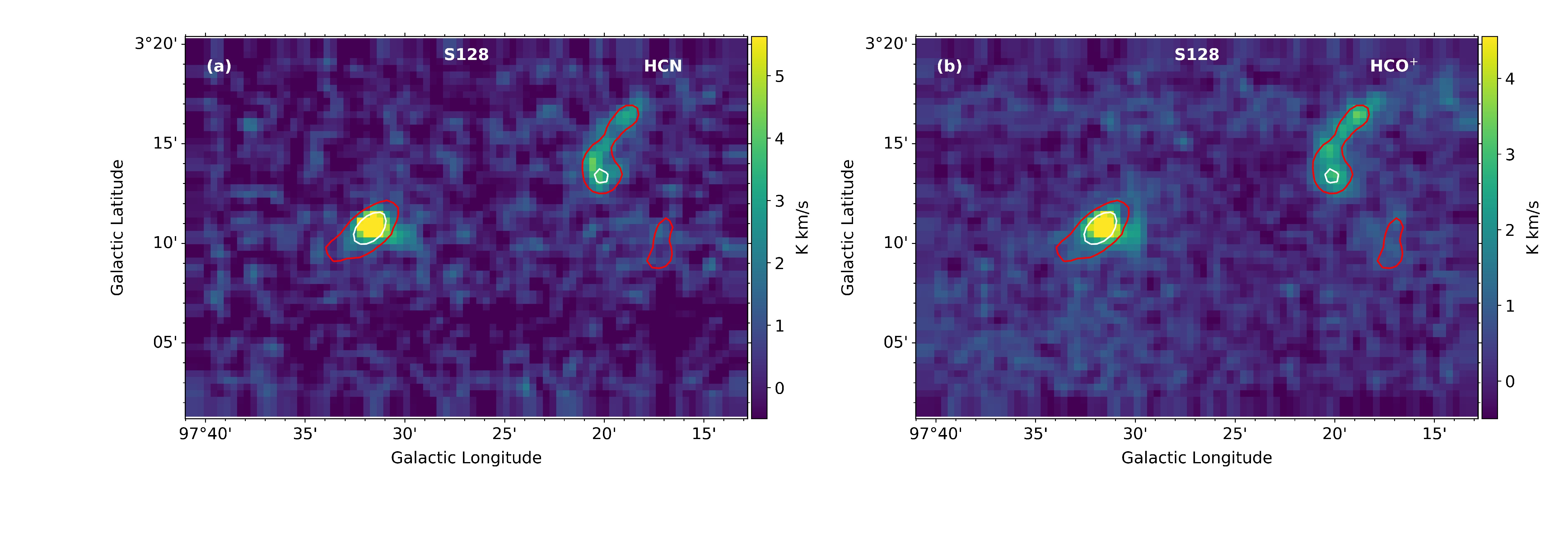
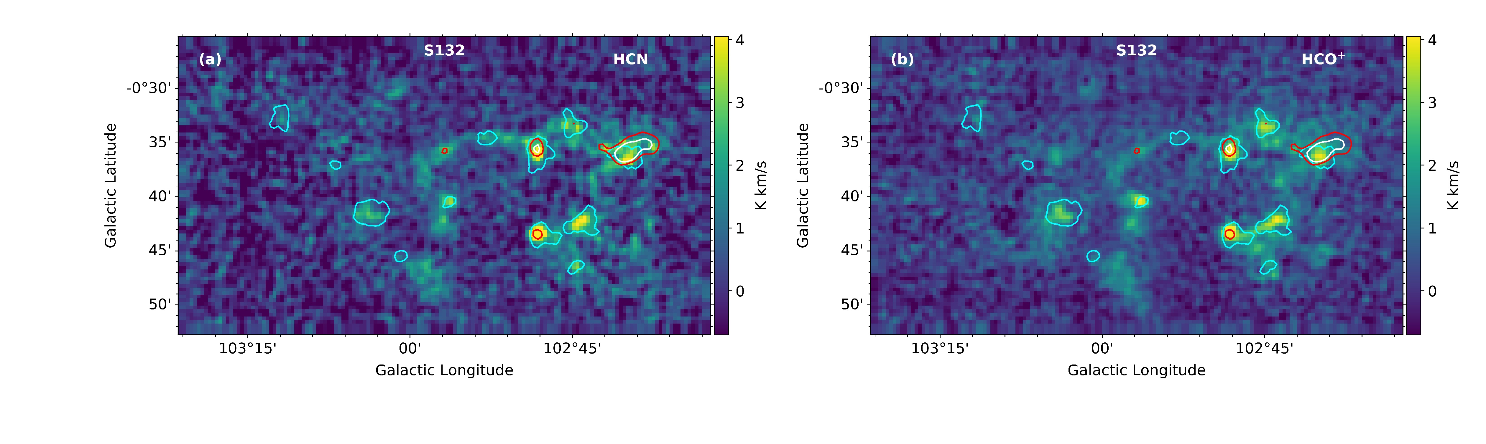
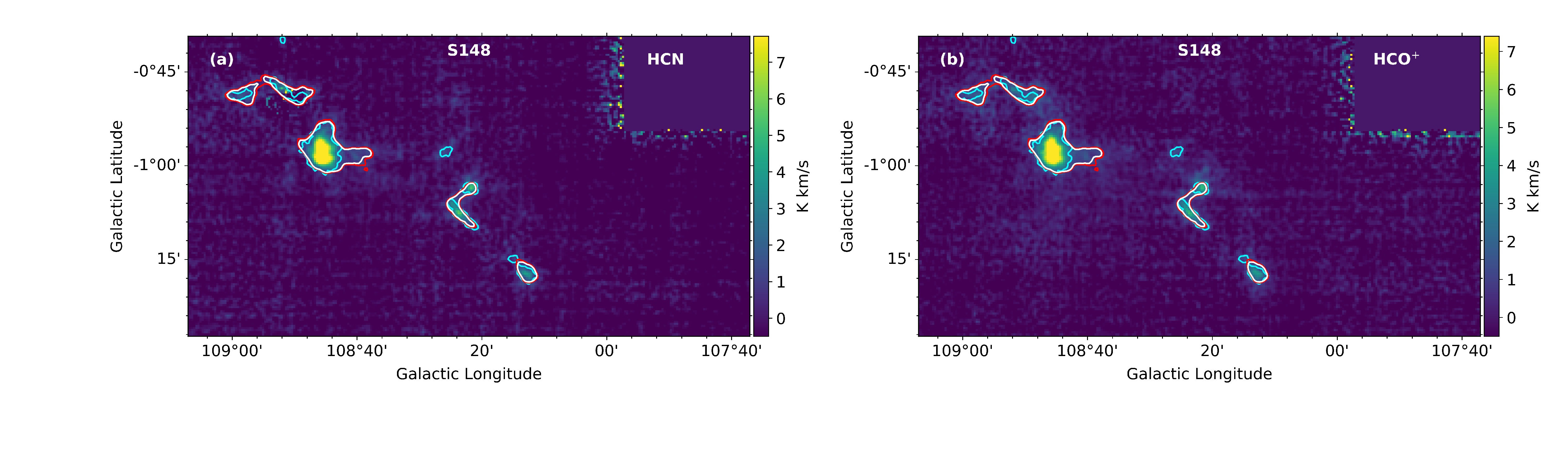
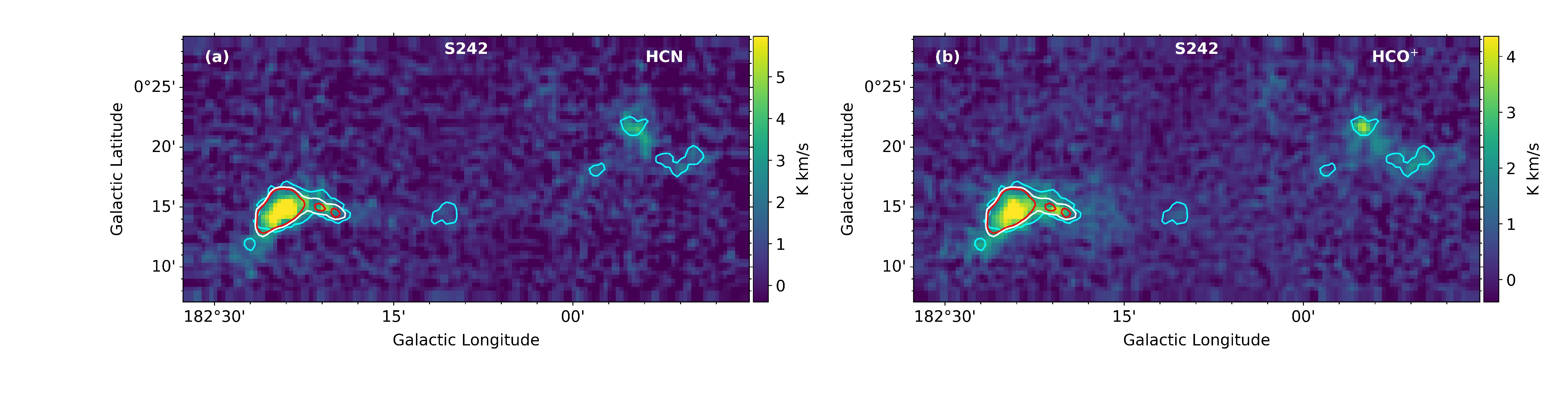
Figure 1: The integrated intensity map of (a) HCN and (b) HCO⁺, respectively, for the new outer Galaxy targets studied in this paper, as identified in each panel. The white contours indicate the $N_{\rm{H_{2}}}\geq 8\times 10^{21}\ \rm{cm^{-2}}$ regions, red contours show the $Z-$corrected column density, $N_{\rm{H_{2}}}^{{}^{\prime}}\geq 8\times 10^{21}\ \rm{cm^{-2}}$ regions, derived from ¹³CO(see Section 4.1.1), and cyan contours indicate the BGPS mask regions. There is no cyan contour in Sh2-128 as it lacks BGPS data.

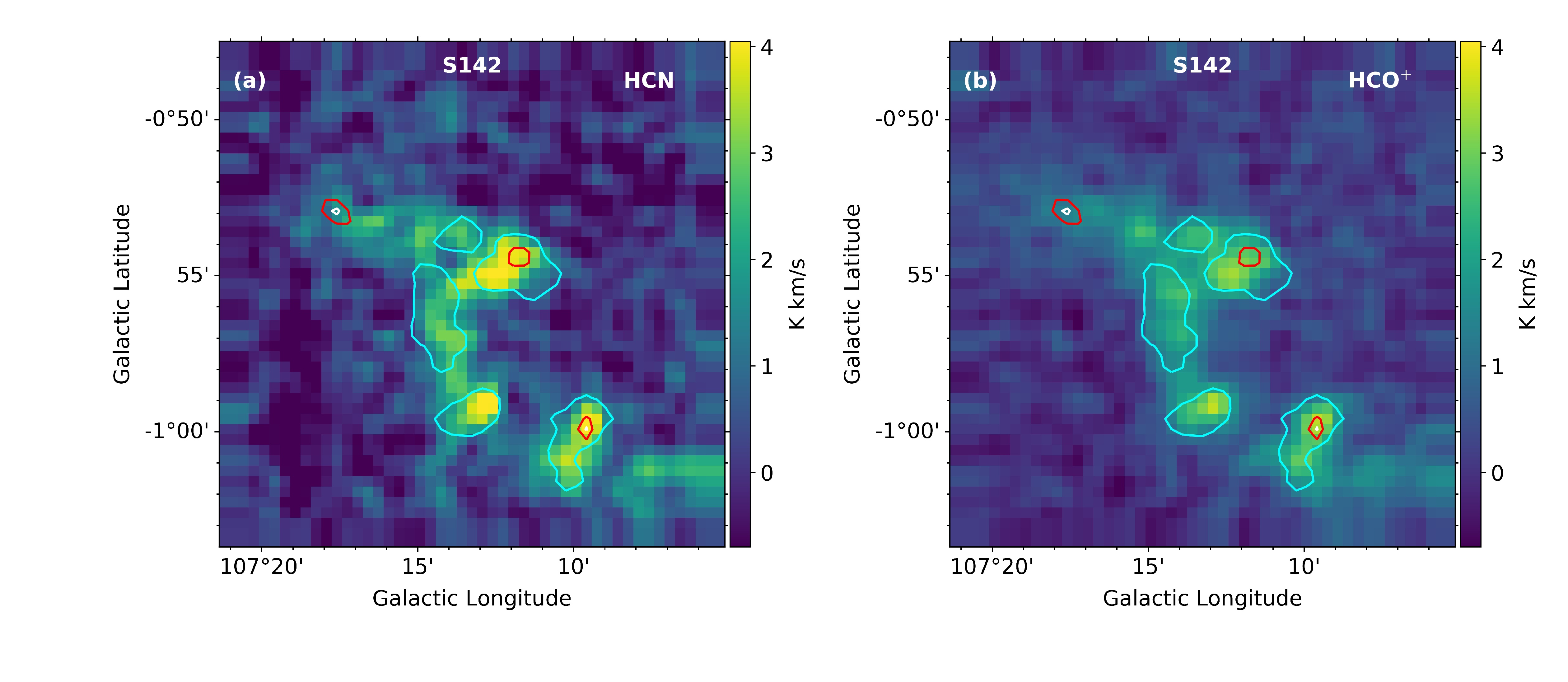
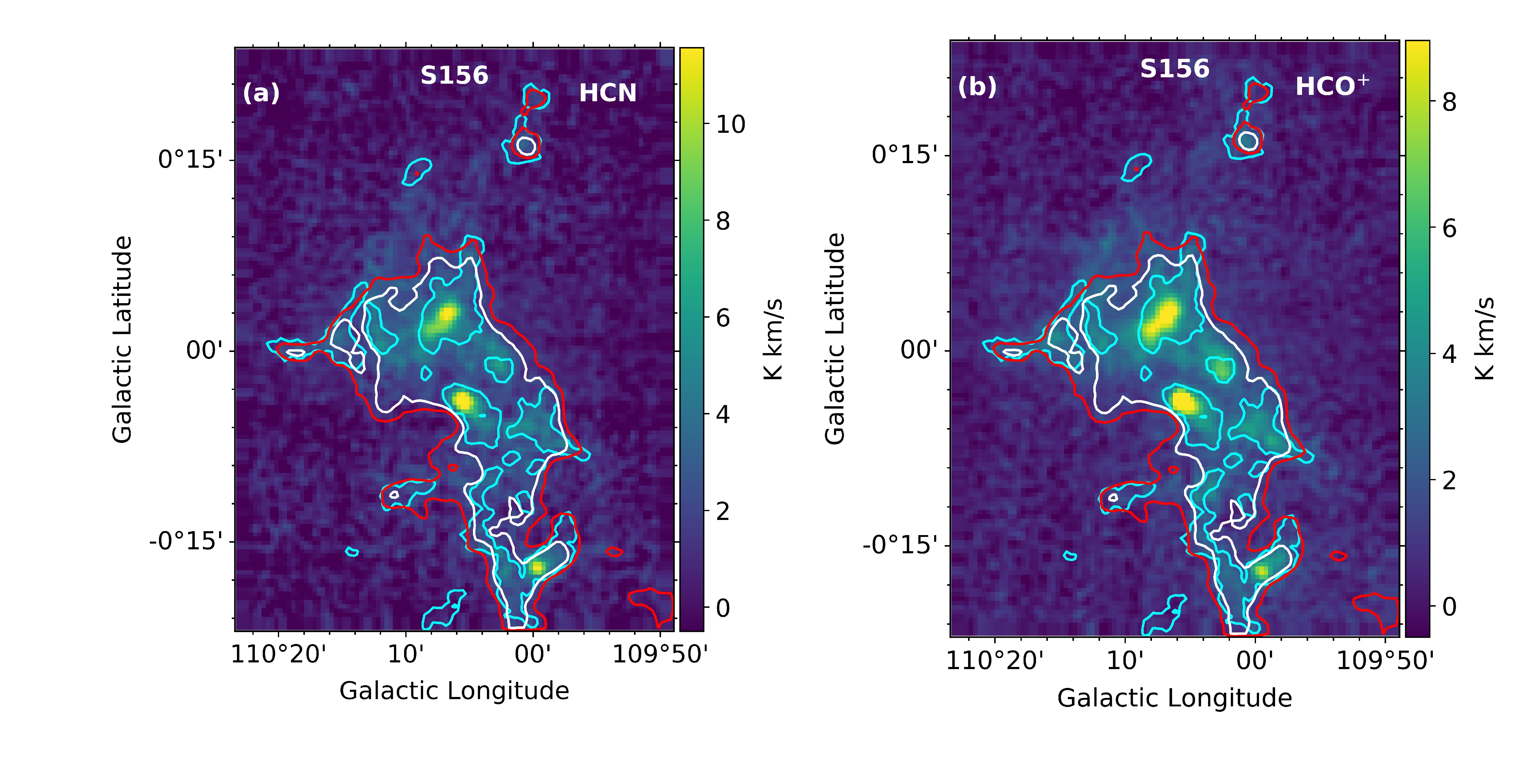
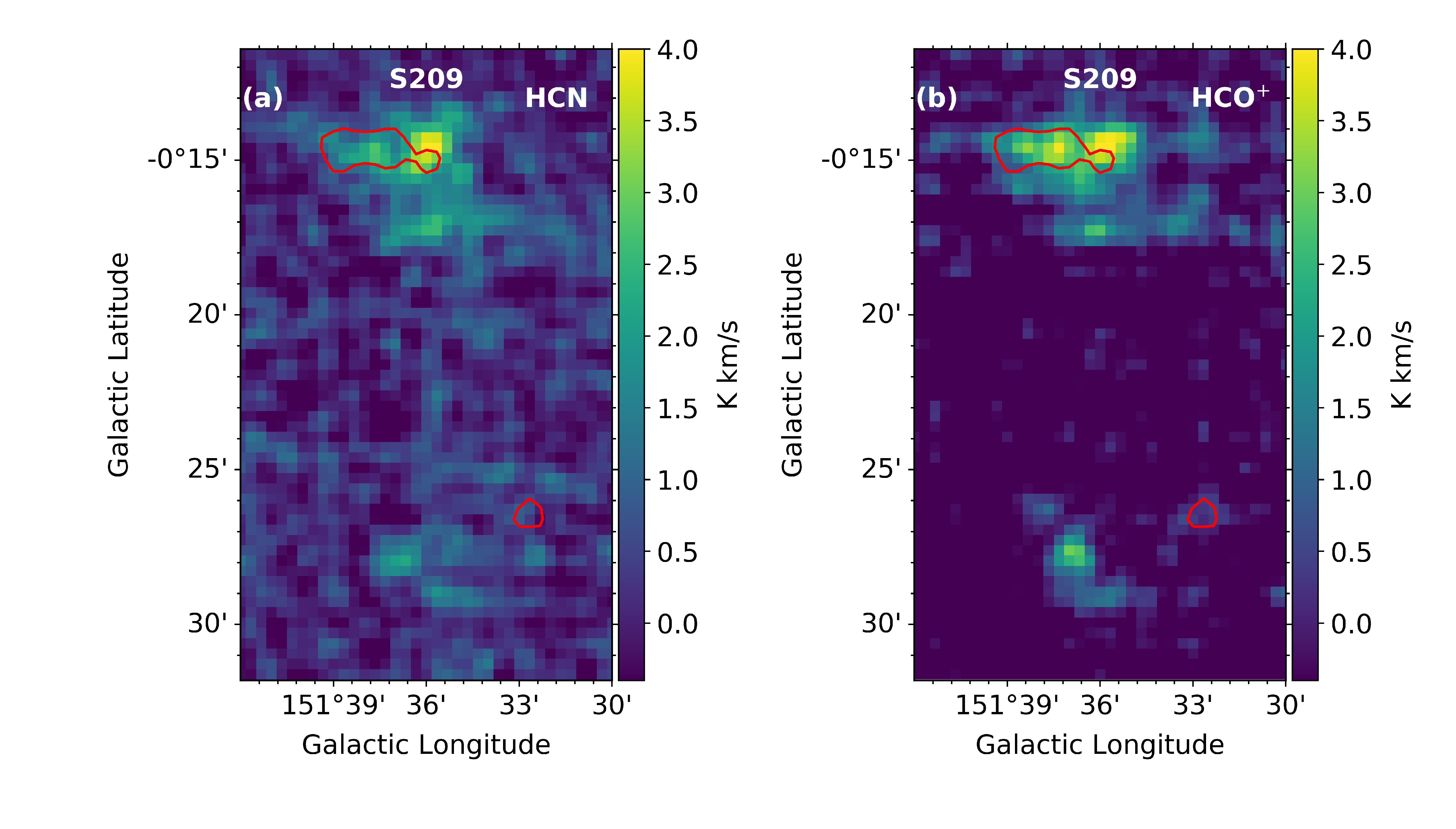
Figure 1: (continued) same as described before. There is no cyan contour in Sh2-209 as it lacks BGPS data and also it has no white contours as there is no region satisfying $N_{\rm{H_{2}}}\geq 8\times 10^{21}\ \rm{cm^{-2}}$.

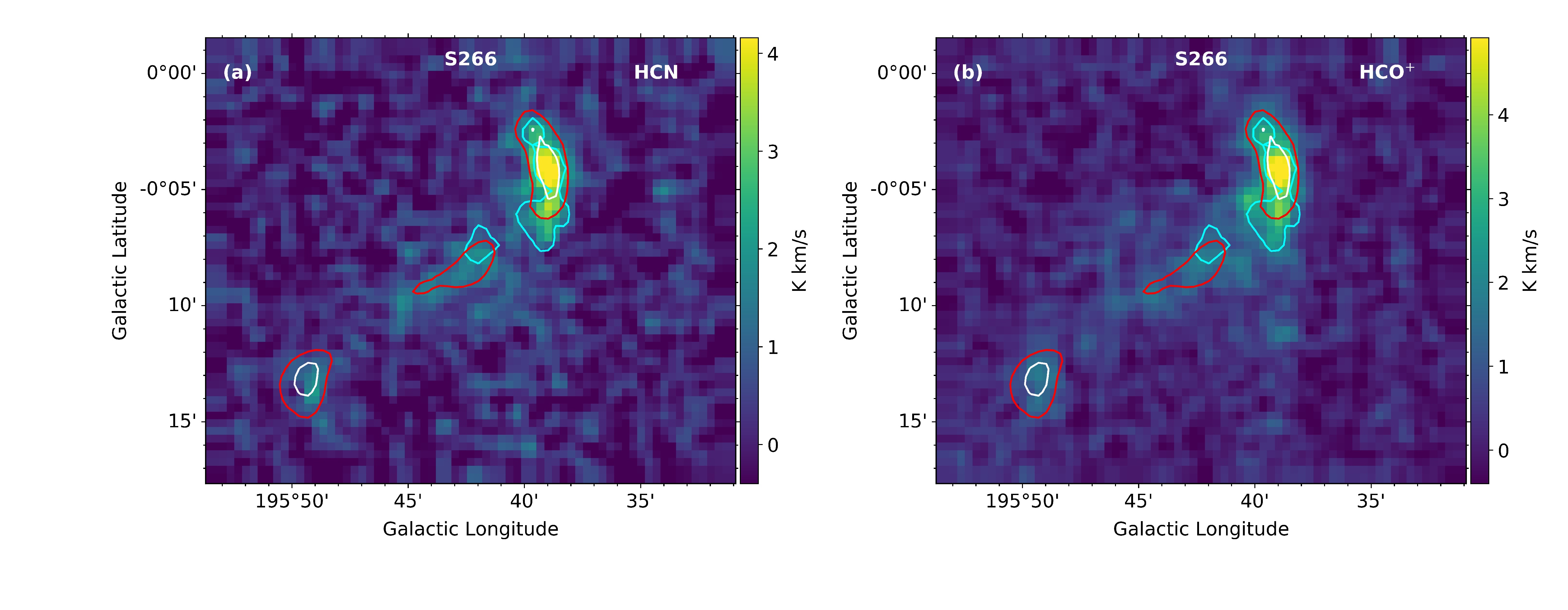
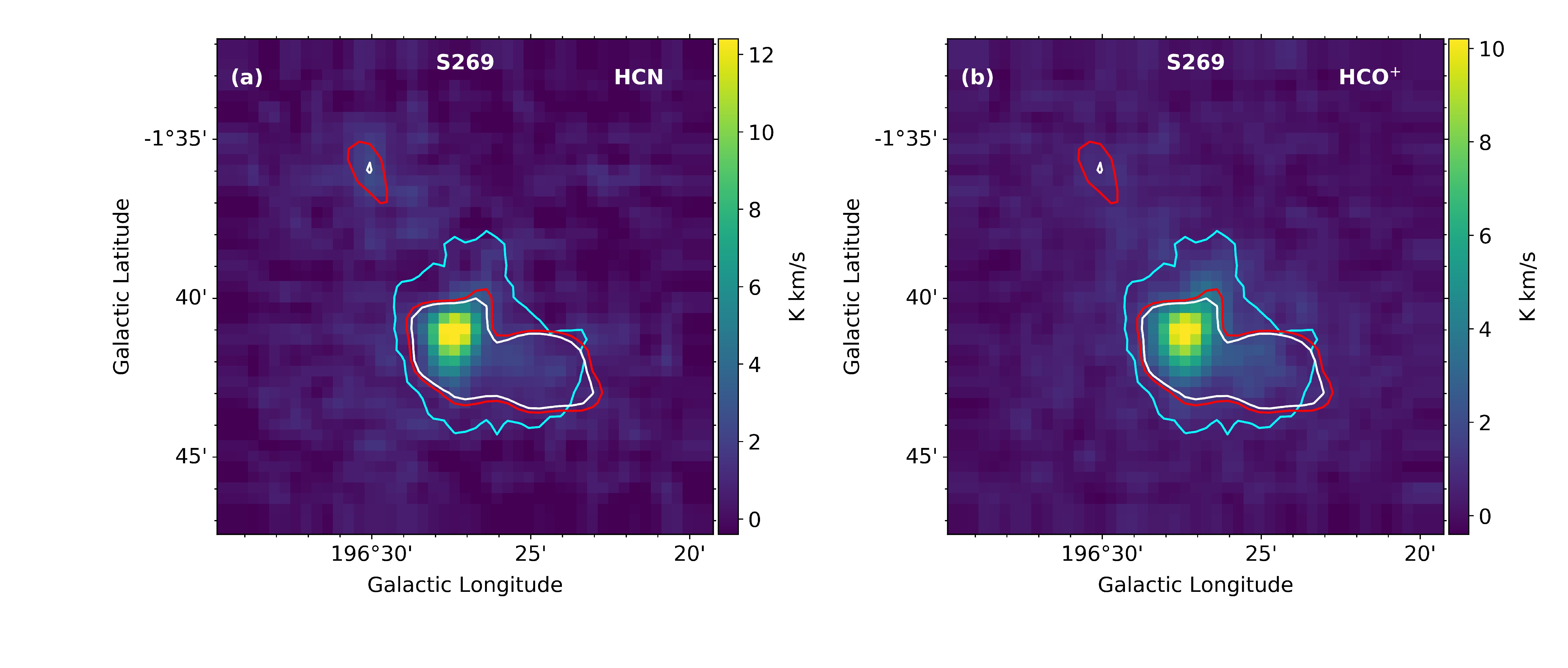
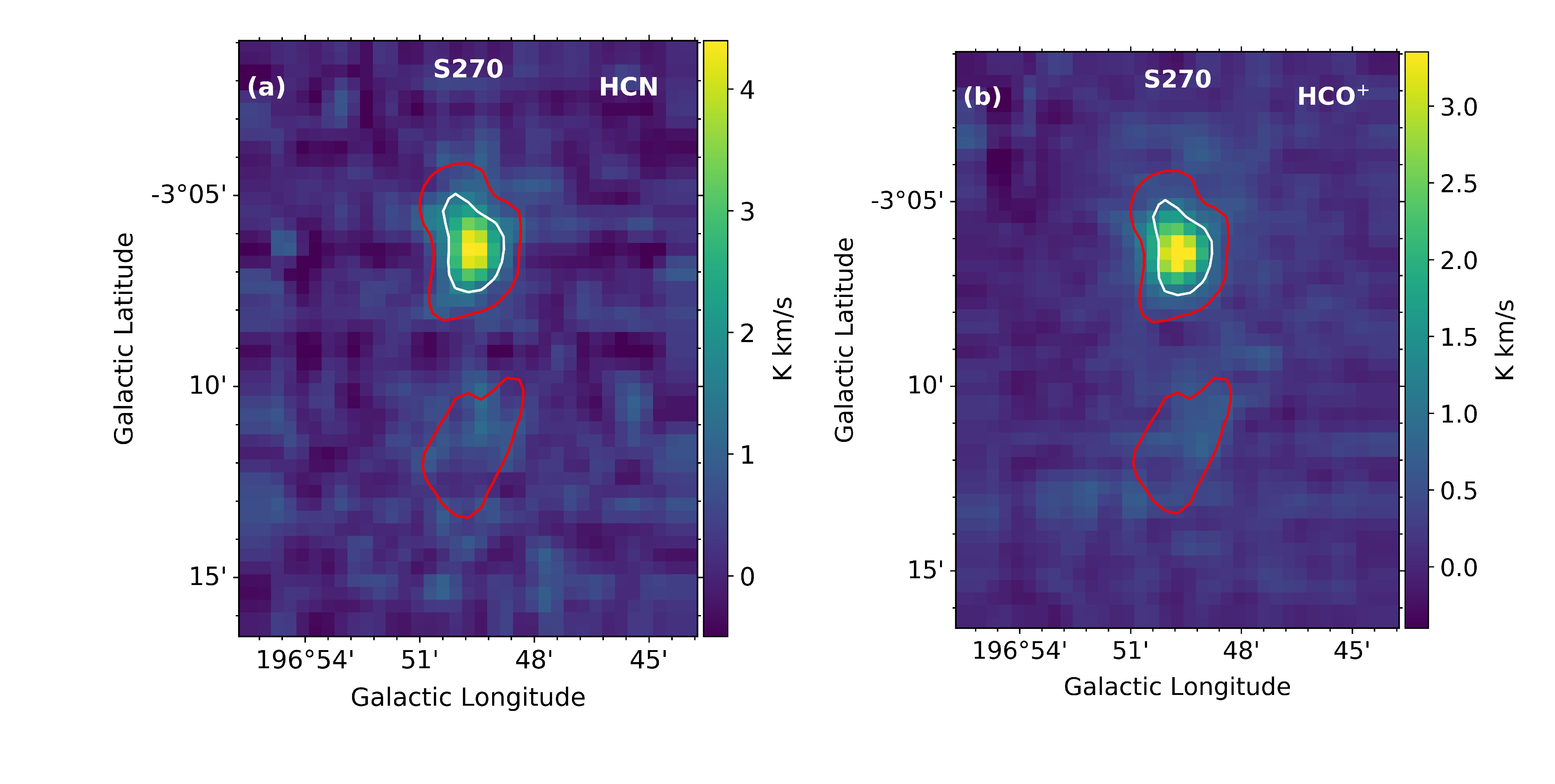
Figure 1: (continued) same as described before. There is no cyan contour in Sh2-270 as it lacks BGPS data.

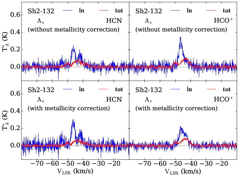
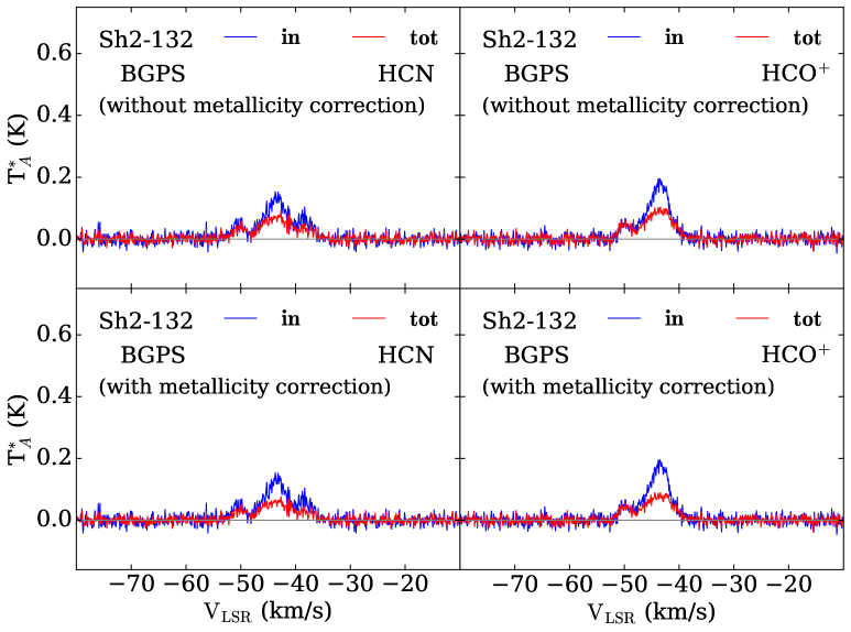
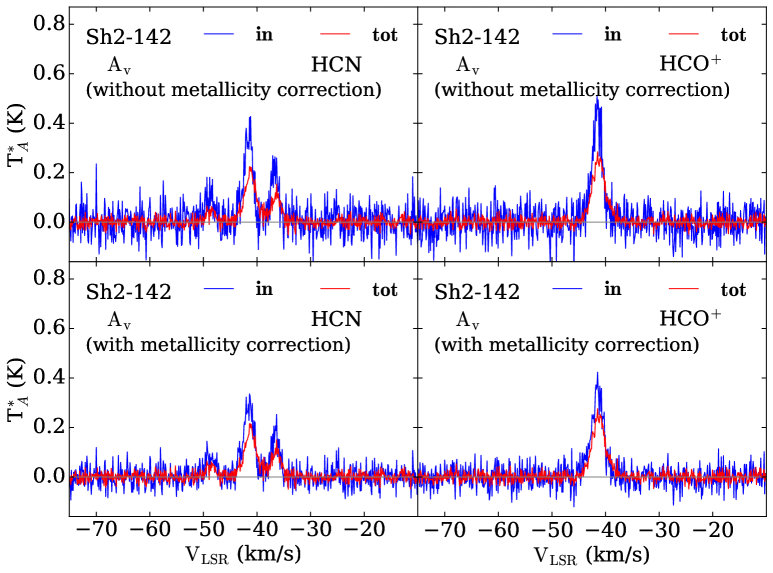
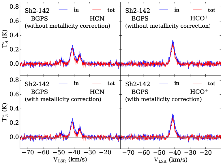
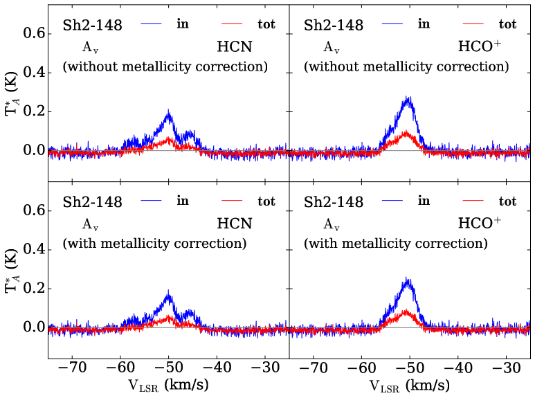
Figure 4: The average spectrum plot for the new outer Galaxy targets studied in this paper, as identified in each panel, based on ‘Gas based analysis’ and ’Dust based analysis’, respectively, with and without metallicity correction. The left panel in all images are for HCN and right panels are for HCO⁺. The blue line indicates the line emission coming from the “in” regions based on gas and dust analysis in the respective images. The red line indicates the emission from the “total” regions. The upper panels of each image show the average spectrum for without metallicity correction case and the bottom panels depict the case after applying the metallicity correction, respectively.

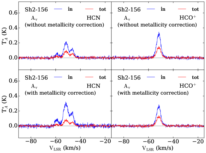
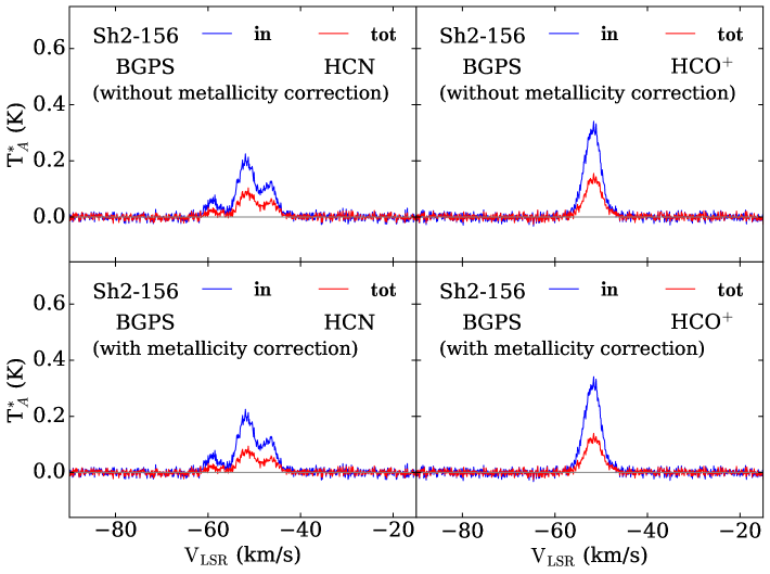
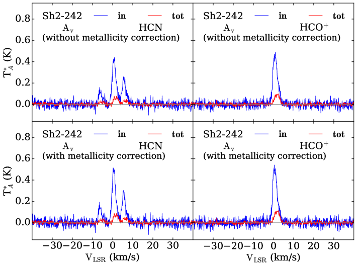
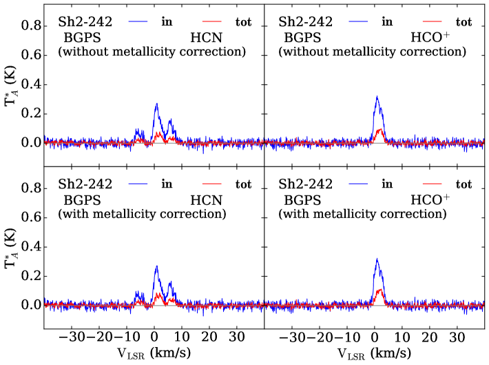
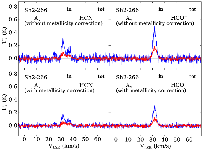
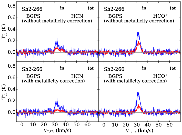
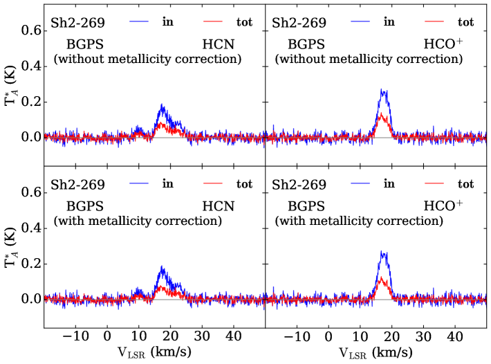
Figure 2: (continued) Same as described earlier for the clouds Sh2-156, Sh2-242, Sh2-266, and Sh2-269.

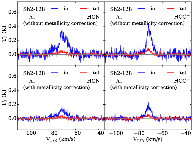
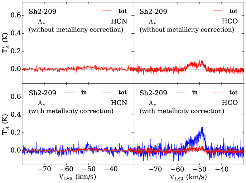
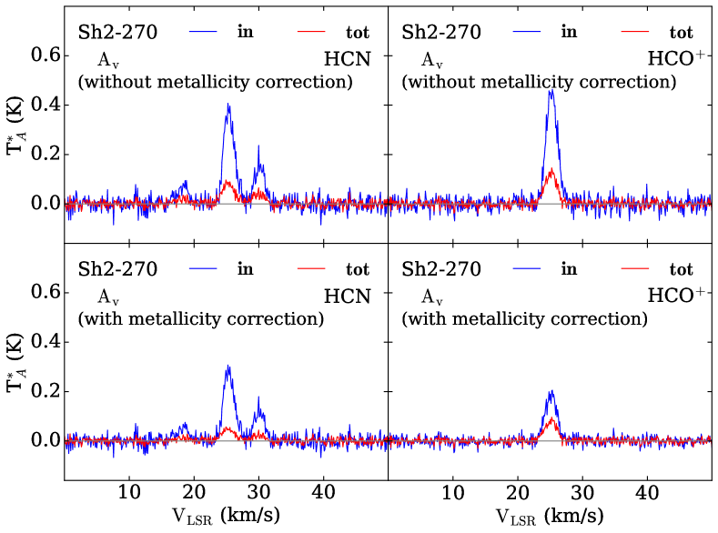
Figure 2: (continued) Same as described earlier for the clouds Sh2-128, Sh2-209, and Sh2-270, based on ‘Gas-based analysis’. The upper panel of Sh2-209 has no blue line because there is no region above $N_{\rm{H_{2}}}\geq 8\times 10^{21}\ \rm{cm^{-2}}$.

4.1.2 Line Luminosity Estimation

To determine the line luminosity of HCN and HCO⁺ within the dense region ($L_{\rm X,in}$), we identified pixels that meet the column density threshold criteria for the “dense” region. To calculate the luminosity from the entire cloud ($L_{\rm X,tot}$), we used the outer boundary condition of column density, $N_{\rm{H_{2}}}\geq 1.5\mbox{${}\times 10^{21}$}\ \rm{cm^{-2}}$. The velocity range for HCO⁺ is the same as for ¹³CO  while for HCN, the velocity range is broader (approximately 3-6 km s^-1 on each side, according to target requirements, as reported in Table A.1) compared to ¹³CO to accommodate the hyperfine structure. Our luminosity and uncertainty in luminosity calculations are based on the method presented in Patra et al. (2022). The luminosity for the dense region is defined as follows

$$L_{\rm X,in}=D^{2}I_{\rm X}N_{\rm in}\Omega_{\rm pix}$$ (7)

where $N_{\rm in}$ represents the number of pixels accounted as “dense” region, $\Omega_{\rm pix}$ denotes the solid angle of a pixel, $D$ is the heliocentric distance of the target in pc and $I_{\rm X}$ is the average integrated intensity for the velocity interval spanning from $v_{\rm sp,l}$ to $v_{\rm sp,u}$, which are the lower and upper limits of the line spectral window. We utilize the spectra (Figure 4) that are averaged over the relevant contours to determine the average integrated intensity.

$$I_{\rm X}=\int_{v_{\rm sp,l}}^{v_{\rm sp,u}}T_{X}dv$$ (8)

We calculated the uncertainty in luminosity using the following equation

$$\sigma_{L}=D^{2}\delta v\sqrt{N_{ch}}\ \sigma_{T_{X}}\ N_{\rm in}\Omega_{\rm pix},$$ (9)

where, $N_{ch}$ and $\delta v$ represents the number of channels within the line region and channel width, respectively, and $\sigma_{T_{X}}$ denotes the rms noise in the baseline of the averaged spectrum. In a similar way, we have estimated the luminosity from the entire cloud ($L_{\rm X,tot}$) by considering the pixels satisfying $N_{\rm{H_{2}}}(\mathrm{and}\ N_{\rm{H_{2}}}^{{}^{\prime}})\geq 1.5\times 10^{21}\ \rm{cm^{-2}}$.

Figure 4 shows the average HCN and HCO⁺ spectrum for the new targets, showing both “in” and “total” regions. The left column presents average spectrum from the gas-based analysis, while the right column shows the dust-based analysis. Sh2-128, Sh2-209, and Sh2-270 are included only in the gas-based analysis. Red lines represent the spectra averaged over the entire cloud, with a column density threshold of $N_{\rm{H_{2}}}(\mathrm{and}\ N_{\rm{H_{2}}}^{{}^{\prime}})\geq 1.5\times 10^{21}\ \rm{cm^{-2}}$ for the top (no metallicity correction) and bottom (with $Z-$correction) panels. The blue lines in the left column represent the spectra averaged over pixels that satisfy the “in” condition based on column density criterion for both the no $Z-$correction (top panel) and with $Z-$correction (bottom panel). In the right column, the blue lines show the average spectrum from the BGPS mask region.

We tabulated the logarithmic values of the luminosity with and without metallicity correction ($L_{\rm Q}$ and $L_{\rm Q}^{{}^{\prime}}$) in Table 3 and 4, respectively. The luminosity values for the “in” region ($L_{\rm in}$) of Sh2-209, Sh2-212, and G037.677+00.155 are not included in Table 3. This omission is due to the absence of pixels with $N_{\rm{H_{2}}}\geq 8\times 10^{21}\ \rm{cm^{-2}}$ when the metallicity correction is not applied. After applying the metallicity correction in the molecular hydrogen column density estimation, G036.459-00.183 and G037.677+00.155 have no pixels satisfying the “dense” condition ($N_{\rm{H_{2}}}^{{}^{\prime}}\geq 8\times 10^{21}\ \rm{cm^{-2}}$), see Table 4. Interestingly, despite the lack of dense pixels, all these sources exhibit significant 24 µm luminosities and are associated with H II regions (Vutisalchavakul et al., 2016), which clearly indicates ongoing or recent star formation. A lack of dense gas now can indicate that star formation is about to pause or end.

Table 3: $M_{\rm dg,Gas}$ versus Luminosities (without metallicity correction)

Source	$\mathrm{Log}\ M_{\rm dg,Gas}$	Log $L_{\rm tot}$	Log $L_{\rm in}$	$\mathrm{Log\ \alpha_{tot}}$	$\mathrm{Log\ \alpha_{in}}$	Log $L_{\rm tot}$	Log $L_{\rm in}$	$\mathrm{Log\ \alpha_{tot}}$	$\mathrm{Log\ \alpha_{in}}$
	(M⊙)	HCN				HCO+
	Outer Galaxy Targets
Sh2-128	$3.35^{+0.11}_{-0.11}$	$2.39^{+0.12}_{-0.11}$	$1.77^{+0.11}_{-0.11}$	$0.96^{+0.12}_{-0.11}$	$1.58^{+0.11}_{-0.11}$	$2.47^{+0.11}_{-0.11}$	$1.65^{+0.11}_{-0.11}$	$0.88^{+0.12}_{-0.11}$	$1.70^{+0.11}_{-0.11}$
Sh2-132	$3.24^{+0.05}_{-0.05}$	$2.57^{+0.05}_{-0.06}$	$1.36^{+0.05}_{-0.06}$	$0.67^{+0.05}_{-0.06}$	$1.88^{+0.05}_{-0.06}$	$2.58^{+0.05}_{-0.06}$	$1.33^{+0.05}_{-0.06}$	$0.66^{+0.05}_{-0.06}$	$1.91^{+0.05}_{-0.06}$
Sh2-142	$1.48^{+0.05}_{-0.05}$	$1.70^{+0.05}_{-0.05}$	$-0.28^{+0.05}_{-0.05}$	$-0.22^{+0.05}_{-0.05}$	$1.76^{+0.05}_{-0.05}$	$1.65^{+0.05}_{-0.05}$	$-0.40^{+0.05}_{-0.05}$	$-0.17^{+0.05}_{-0.05}$	$1.88^{+0.05}_{-0.05}$
Sh2-148	$4.46^{+0.05}_{-0.05}$	$2.43^{+0.05}_{-0.05}$	$2.31^{+0.05}_{-0.05}$	$2.03^{+0.05}_{-0.05}$	$2.15^{+0.05}_{-0.05}$	$2.57^{+0.05}_{-0.05}$	$2.30^{+0.05}_{-0.05}$	$1.89^{+0.05}_{-0.05}$	$2.09^{+0.05}_{-0.05}$
Sh2-156	$4.46^{+0.07}_{-0.07}$	$2.82^{+0.07}_{-0.07}$	$2.54^{+0.07}_{-0.07}$	$1.64^{+0.07}_{-0.07}$	$1.92^{+0.07}_{-0.07}$	$2.81^{+0.07}_{-0.07}$	$2.52^{+0.07}_{-0.07}$	$1.65^{+0.07}_{-0.07}$	$1.94^{+0.07}_{-0.07}$
Sh2-209	$\cdots$	$2.09^{+0.07}_{-0.08}$	$\cdots$	$\cdots$	$\cdots$	$2.39^{+0.06}_{-0.07}$	$\cdots$	$\cdots$	$\cdots$
Sh2-242	$2.97^{+0.02}_{-0.02}$	$1.61^{+0.03}_{-0.02}$	$1.08^{+0.02}_{-0.02}$	$1.36^{+0.03}_{-0.02}$	$1.89^{+0.02}_{-0.02}$	$1.55^{+0.03}_{-0.02}$	$0.94^{+0.02}_{-0.02}$	$1.42^{+0.03}_{-0.02}$	$2.03^{+0.02}_{-0.02}$
Sh2-266	$3.09^{+0.09}_{-0.11}$	$1.96^{+0.09}_{-0.11}$	$1.25^{+0.09}_{-0.11}$	$1.13^{+0.09}_{-0.11}$	$1.84^{+0.09}_{-0.11}$	$2.06^{+0.09}_{-0.11}$	$1.30^{+0.09}_{-0.11}$	$1.03^{+0.09}_{-0.11}$	$1.79^{+0.09}_{-0.11}$
Sh2-269	$3.77^{+0.07}_{-0.07}$	$2.09^{+0.07}_{-0.07}$	$1.80^{+0.07}_{-0.07}$	$1.68^{+0.07}_{-0.07}$	$1.97^{+0.07}_{-0.07}$	$2.07^{+0.07}_{-0.07}$	$1.77^{+0.07}_{-0.07}$	$1.70^{+0.07}_{-0.07}$	$2.00^{+0.07}_{-0.07}$
Sh2-270	$3.62^{+0.12}_{-0.17}$	$2.11^{+0.12}_{-0.17}$	$1.64^{+0.12}_{-0.17}$	$1.51^{+0.12}_{-0.17}$	$1.98^{+0.12}_{-0.17}$	$2.03^{+0.12}_{-0.17}$	$1.54^{+0.12}_{-0.17}$	$1.59^{+0.12}_{-0.17}$	$2.08^{+0.12}_{-0.17}$
	Outer Galaxy Targets from Patra et al. (2022)
Sh2-206	$3.02^{+0.05}_{-0.05}$	$1.88^{+0.05}_{-0.05}$	$1.14^{+0.05}_{-0.05}$	$1.14^{+0.05}_{-0.05}$	$1.88^{+0.05}_{-0.05}$	$1.84^{+0.05}_{-0.05}$	$1.05^{+0.05}_{-0.05}$	$1.18^{+0.05}_{-0.05}$	$1.97^{+0.05}_{-0.05}$
Sh2-208	$2.58^{+0.05}_{-0.06}$	$1.31^{+0.06}_{-0.06}$	$0.63^{+0.06}_{-0.06}$	$1.27^{+0.06}_{-0.06}$	$1.95^{+0.06}_{-0.06}$	$1.39^{+0.05}_{-0.06}$	$0.62^{+0.05}_{-0.06}$	$1.19^{+0.06}_{-0.06}$	$1.96^{+0.06}_{-0.06}$
Sh2-212	$\cdots$	$1.89^{+0.15}_{-0.21}$	$\cdots$	$\cdots$	$\cdots$	$1.95^{+0.15}_{-0.21}$	$\cdots$	$\cdots$	$\cdots$
Sh2-228	$1.84^{+0.03}_{-0.03}$	$1.40^{+0.05}_{-0.05}$	$-0.44^{+0.08}_{-0.09}$	$0.44^{+0.05}_{-0.05}$	$2.28^{+0.08}_{-0.09}$	$1.29^{+0.04}_{-0.05}$	$-0.74^{+0.10}_{-0.13}$	$0.55^{+0.05}_{-0.05}$	$2.59^{+0.08}_{-0.09}$
Sh2-235	$3.89^{+0.03}_{-0.04}$	$2.45^{+0.04}_{-0.04}$	$2.18^{+0.03}_{-0.04}$	$1.44^{+0.04}_{-0.04}$	$1.71^{+0.03}_{-0.04}$	$2.43^{+0.03}_{-0.04}$	$2.10^{+0.03}_{-0.04}$	$1.46^{+0.03}_{-0.04}$	$1.79^{+0.03}_{-0.04}$
Sh2-252	$4.33^{+0.05}_{-0.05}$	$2.53^{+0.05}_{-0.05}$	$2.35^{+0.05}_{-0.05}$	$1.80^{+0.05}_{-0.05}$	$1.98^{+0.05}_{-0.05}$	$2.48^{+0.05}_{-0.05}$	$2.27^{+0.05}_{-0.05}$	$1.85^{+0.05}_{-0.05}$	$2.06^{+0.05}_{-0.05}$
Sh2-254	$3.91^{+0.05}_{-0.04}$	$2.50^{+0.05}_{-0.04}$	$2.16^{+0.05}_{-0.04}$	$1.41^{+0.05}_{-0.04}$	$1.75^{+0.05}_{-0.04}$	$2.50^{+0.05}_{-0.04}$	$2.06^{+0.05}_{-0.04}$	$1.41^{+0.05}_{-0.04}$	$1.85^{+0.05}_{-0.04}$
	Inner Galaxy Targets from Evans et al. (2020)
G034.997+00.330	$4.51^{+0.03}_{-0.04}$	$3.25^{+0.03}_{-0.04}$	$2.80^{+0.03}_{-0.04}$	$1.26^{+0.03}_{-0.04}$	$1.71^{+0.03}_{-0.04}$	$3.20^{+0.03}_{-0.04}$	$2.68^{+0.03}_{-0.04}$	$1.31^{+0.03}_{-0.04}$	$1.83^{+0.03}_{-0.04}$
G036.459-00.183	$2.72^{+0.05}_{-0.06}$	$2.80^{+0.05}_{-0.07}$	$0.75^{+0.06}_{-0.08}$	$-0.08^{+0.05}_{-0.07}$	$1.97^{+0.06}_{-0.08}$	$2.71^{+0.05}_{-0.07}$	$0.82^{+0.06}_{-0.07}$	$0.01^{+0.05}_{-0.07}$	$1.90^{+0.06}_{-0.07}$
G037.677+00.155	$\cdots$	$2.12^{+0.03}_{-0.04}$	$\cdots$		$\cdots$	$1.94^{+0.03}_{-0.03}$	$\cdots$	$\cdots$	$\cdots$
G045.825-00.291	$4.49^{+0.05}_{-0.07}$	$3.02^{+0.05}_{-0.08}$	$2.41^{+0.05}_{-0.07}$	$1.47^{+0.05}_{-0.08}$	$2.08^{+0.05}_{-0.07}$	$2.85^{+0.06}_{-0.08}$	$2.17^{+0.06}_{-0.08}$	$1.64^{+0.06}_{-0.08}$	$2.32^{+0.06}_{-0.08}$
G046.495-00.241	$3.30^{+0.14}_{-0.17}$	$2.24^{+0.14}_{-0.17}$	$1.43^{+0.14}_{-0.17}$	$1.06^{+0.14}_{-0.17}$	$1.87^{+0.14}_{-0.17}$	$2.14^{+0.14}_{-0.17}$	$1.34^{+0.14}_{-0.17}$	$1.16^{+0.14}_{-0.17}$	$1.96^{+0.14}_{-0.17}$

Note. — 1. Units of luminosities are K km s^-1pc².

2. Units of conversion factors are $\mbox{M${}_{\odot}$}\ (\rm K\ km\ s^{-1}\ pc^{2})^{-1}$.

3. Sh2-142, Sh2-228, and G036.459-00.183 have fewer than 9 pixels meeting the column density criterion for dense region, hence excluded for reliability.

Table 4: $M_{\rm dg,Gas}^{{}^{\prime}}$ versus Luminosities (with metallicity correction)

Source	$\mathrm{Log}\ M_{\rm dg,Gas}^{{}^{\prime}}$	Log $L_{\rm tot}^{{}^{\prime}}$	Log $L_{\rm in}^{{}^{\prime}}$	$\mathrm{Log\ \alpha^{\prime}_{tot}}$	$\mathrm{Log\ \alpha^{\prime}_{in}}$	Log $L_{\rm tot}^{{}^{\prime}}$	Log $L_{\rm in}^{{}^{\prime}}$	$\mathrm{Log\ \alpha^{\prime}_{tot}}$	$\mathrm{Log\ \alpha^{\prime}_{in}}$
	(M⊙)	HCN				HCO+
	Outer Galaxy Targets
Sh2-128	$4.23^{+0.11}_{-0.11}$	$2.45^{+0.12}_{-0.12}$	$2.21^{+0.11}_{-0.11}$	$1.78^{+0.12}_{-0.12}$	$2.02^{+0.11}_{-0.11}$	$2.61^{+0.12}_{-0.11}$	$2.14^{+0.11}_{-0.11}$	$1.62^{+0.12}_{-0.11}$	$2.09^{+0.11}_{-0.11}$
Sh2-132	$3.69^{+0.05}_{-0.05}$	$2.62^{+0.05}_{-0.05}$	$1.77^{+0.05}_{-0.06}$	$1.06^{+0.05}_{-0.05}$	$1.92^{+0.05}_{-0.06}$	$2.65^{+0.05}_{-0.06}$	$1.68^{+0.05}_{-0.06}$	$1.04^{+0.05}_{-0.06}$	$2.01^{+0.05}_{-0.06}$
Sh2-142	$2.32^{+0.05}_{-0.05}$	$1.72^{+0.05}_{-0.05}$	$0.47^{+0.05}_{-0.05}$	$0.60^{+0.05}_{-0.05}$	$1.84^{+0.05}_{-0.05}$	$1.67^{+0.05}_{-0.05}$	$0.37^{+0.05}_{-0.05}$	$0.65^{+0.05}_{-0.05}$	$1.95^{+0.05}_{-0.05}$
Sh2-148	$4.56^{+0.05}_{-0.05}$	$2.42^{+0.05}_{-0.05}$	$2.34^{+0.05}_{-0.05}$	$2.14^{+0.05}_{-0.05}$	$2.22^{+0.05}_{-0.05}$	$2.58^{+0.05}_{-0.05}$	$2.41^{+0.05}_{-0.05}$	$1.98^{+0.05}_{-0.05}$	$2.15^{+0.05}_{-0.05}$
Sh2-156	$4.74^{+0.07}_{-0.07}$	$2.83^{+0.07}_{-0.07}$	$2.66^{+0.07}_{-0.07}$	$1.91^{+0.07}_{-0.07}$	$2.08^{+0.07}_{-0.07}$	$2.83^{+0.07}_{-0.07}$	$2.63^{+0.07}_{-0.07}$	$1.91^{+0.07}_{-0.07}$	$2.11^{+0.07}_{-0.07}$
Sh2-209	$3.85^{+0.06}_{-0.07}$	$2.67^{+0.07}_{-0.08}$	$1.16^{+0.10}_{-0.12}$	$1.18^{+0.07}_{-0.08}$	$2.69^{+0.10}_{-0.12}$	$2.51^{+0.07}_{-0.09}$	$1.90^{+0.06}_{-0.07}$	$1.33^{+0.07}_{-0.09}$	$1.95^{+0.06}_{-0.07}$
Sh2-242	$2.78^{+0.02}_{-0.02}$	$1.59^{+0.03}_{-0.02}$	$0.97^{+0.02}_{-0.02}$	$1.19^{+0.03}_{-0.02}$	$1.80^{+0.02}_{-0.02}$	$1.52^{+0.02}_{-0.02}$	$0.81^{+0.02}_{-0.02}$	$1.26^{+0.02}_{-0.02}$	$1.97^{+0.02}_{-0.02}$
Sh2-266	$3.89^{+0.09}_{-0.11}$	$2.06^{+0.09}_{-0.11}$	$1.71^{+0.09}_{-0.11}$	$1.83^{+0.09}_{-0.11}$	$2.18^{+0.09}_{-0.11}$	$2.20^{+0.09}_{-0.11}$	$1.78^{+0.09}_{-0.11}$	$1.69^{+0.09}_{-0.11}$	$2.11^{+0.09}_{-0.11}$
Sh2-269	$3.90^{+0.07}_{-0.07}$	$2.10^{+0.07}_{-0.07}$	$1.85^{+0.07}_{-0.07}$	$1.80^{+0.07}_{-0.07}$	$2.05^{+0.07}_{-0.07}$	$2.09^{+0.07}_{-0.07}$	$1.81^{+0.07}_{-0.07}$	$1.81^{+0.07}_{-0.07}$	$2.09^{+0.07}_{-0.07}$
Sh2-270	$4.44^{+0.12}_{-0.17}$	$2.21^{+0.12}_{-0.17}$	$1.96^{+0.12}_{-0.17}$	$2.23^{+0.12}_{-0.17}$	$2.48^{+0.12}_{-0.17}$	$2.16^{+0.12}_{-0.17}$	$1.86^{+0.12}_{-0.17}$	$2.27^{+0.12}_{-0.17}$	$2.58^{+0.12}_{-0.17}$
	Outer Galaxy Targets from Patra et al. (2022)
Sh2-206	$3.27^{+0.05}_{-0.05}$	$1.93^{+0.05}_{-0.05}$	$1.27^{+0.05}_{-0.05}$	$1.34^{+0.05}_{-0.05}$	$2.00^{+0.05}_{-0.05}$	$1.89^{+0.05}_{-0.05}$	$1.19^{+0.05}_{-0.05}$	$1.38^{+0.05}_{-0.05}$	$2.07^{+0.05}_{-0.05}$
Sh2-208	$2.73^{+0.05}_{-0.06}$	$1.33^{+0.06}_{-0.06}$	$0.85^{+0.06}_{-0.06}$	$1.40^{+0.06}_{-0.06}$	$1.88^{+0.06}_{-0.06}$	$1.43^{+0.05}_{-0.06}$	$0.84^{+0.05}_{-0.06}$	$1.30^{+0.05}_{-0.06}$	$1.89^{+0.05}_{-0.06}$
Sh2-212	$1.88^{+0.22}_{-0.43}$	$1.96^{+0.15}_{-0.21}$	$0.08^{+0.15}_{-0.21}$	$-0.08^{+0.15}_{-0.21}$	$1.79^{+0.15}_{-0.21}$	$2.03^{+0.15}_{-0.21}$	$0.04^{+0.15}_{-0.21}$	$-0.15^{+0.15}_{-0.21}$	$1.84^{+0.15}_{-0.21}$
Sh2-228	$2.87^{+0.03}_{-0.03}$	$1.42^{+0.05}_{-0.06}$	$0.60^{+0.04}_{-0.05}$	$1.45^{+0.05}_{-0.06}$	$2.27^{+0.04}_{-0.05}$	$1.32^{+0.05}_{-0.05}$	$0.51^{+0.04}_{-0.04}$	$1.55^{+0.05}_{-0.05}$	$2.36^{+0.04}_{-0.04}$
Sh2-235	$4.03^{+0.03}_{-0.04}$	$2.45^{+0.04}_{-0.04}$	$2.22^{+0.03}_{-0.04}$	$1.57^{+0.04}_{-0.04}$	$1.80^{+0.03}_{-0.04}$	$2.44^{+0.04}_{-0.04}$	$2.16^{+0.03}_{-0.04}$	$1.58^{+0.04}_{-0.04}$	$1.87^{+0.03}_{-0.04}$
Sh2-252	$4.32^{+0.05}_{-0.05}$	$2.53^{+0.05}_{-0.05}$	$2.34^{+0.05}_{-0.05}$	$1.79^{+0.05}_{-0.05}$	$1.97^{+0.05}_{-0.05}$	$2.48^{+0.05}_{-0.05}$	$2.26^{+0.05}_{-0.05}$	$1.83^{+0.05}_{-0.05}$	$2.05^{+0.05}_{-0.05}$
Sh2-254	$4.09^{+0.05}_{-0.04}$	$2.51^{+0.05}_{-0.04}$	$2.23^{+0.05}_{-0.04}$	$1.58^{+0.05}_{-0.04}$	$1.86^{+0.05}_{-0.04}$	$2.51^{+0.05}_{-0.04}$	$2.15^{+0.05}_{-0.04}$	$1.57^{+0.05}_{-0.04}$	$1.94^{+0.05}_{-0.04}$
	Inner Galaxy Targets from Evans et al. (2020)
G034.997+00.330	$4.13^{+0.03}_{-0.04}$	$3.23^{+0.03}_{-0.04}$	$2.57^{+0.03}_{-0.04}$	$0.90^{+0.03}_{-0.04}$	$1.56^{+0.03}_{-0.04}$	$3.17^{+0.03}_{-0.04}$	$2.42^{+0.03}_{-0.04}$	$0.96^{+0.03}_{-0.04}$	$1.71^{+0.03}_{-0.04}$
G036.459-00.183	$\cdots$	$2.76^{+0.05}_{-0.07}$	$\cdots$	$\cdots$	$\cdots$	$2.68^{+0.05}_{-0.07}$	$\cdots$	$\cdots$	$\cdots$
G037.677+00.155	$\cdots$	$2.02^{+0.03}_{-0.03}$	$\cdots$	$\cdots$	$\cdots$	$1.87^{+0.03}_{-0.03}$	$\cdots$	$\cdots$	$\cdots$
G045.825-00.291	$4.25^{+0.05}_{-0.07}$	$3.00^{+0.05}_{-0.08}$	$2.23^{+0.05}_{-0.07}$	$1.25^{+0.05}_{-0.08}$	$2.02^{+0.05}_{-0.07}$	$2.83^{+0.06}_{-0.08}$	$2.01^{+0.06}_{-0.08}$	$1.41^{+0.06}_{-0.08}$	$2.24^{+0.06}_{-0.08}$
G046.495-00.241	$3.01^{+0.14}_{-0.17}$	$2.23^{+0.14}_{-0.17}$	$1.19^{+0.14}_{-0.17}$	$0.78^{+0.14}_{-0.17}$	$1.82^{+0.14}_{-0.17}$	$2.12^{+0.14}_{-0.17}$	$1.09^{+0.14}_{-0.17}$	$0.89^{+0.14}_{-0.17}$	$1.92^{+0.14}_{-0.17}$

Note. — 1. Units of luminosities are K km s^-1pc².

2. Units of conversion factors are $\mbox{M${}_{\odot}$}\ (\rm K\ km\ s^{-1}\ pc^{2})^{-1}$.

3. Sh2-212 has only 1 pixel meeting the column density criterion for dense region, hence excluded for reliability.

4.1.3 Dense Gas Mass Measurement

We have calculated the mass of dense gas by considering the pixels satisfying the “dense” condition ($N_{\rm{H_{2}}}(\mathrm{and}\ N_{\rm{H_{2}}}^{{}^{\prime}})\geq 8\times 10^{21}\ \rm{cm^{-2}}$), with and without metallicity correction. The calculation of dense gas mass ($M_{\rm dg,Gas}$) from the gas based analysis is performed using the following equation.

$$M_{\rm dg,Gas}=\mu_{\rm H_{2}}m_{\rm H}A_{\rm pix}\Sigma N_{\rm H_{2}}$$ (10)

where $\mu_{\rm H_{2}}$ is the mean molecular weight, which is 2.809 (Evans et al., 2022), $m_{\rm H}$ is the mass of the hydrogen atom, $A_{\rm pix}$ is the area of a pixel in $\rm cm^{2}$ and $\Sigma N_{\rm H_{2}}$ is the sum of molecular hydrogen column density satisfying the condition for the “dense” region. The dense gas mass values in logarithmic scale for all the targets are listed in Table 3. However, Sh2-142, Sh2-228, and G036.459-00.183 have only 2, 6 and 4 pixels satisfying the above criterion. We have excluded clouds with less than 9 pixels satisfying the column density criterion, providing sufficient resolution of the emission region to ensure the reliability and statistical significance of our analysis.

The metallicity-corrected mass values are obtained using the following equation

$$M_{\rm dg,Gas}^{{}^{\prime}}=\mu_{\rm H_{2}}m_{\rm H}A_{\rm pix}\Sigma N_{\rm H_{2}}^{{}^{\prime}}$$ (11)

where $N_{\rm H_{2}}^{{}^{\prime}}$ corresponds to the molecular hydrogen column density after applying the metallicity correction. We have excluded Sh2-212 because only one pixel meets the “dense” criterion. We tabulated the logarithmic values of $M_{\rm dg,Gas}^{{}^{\prime}}$ in Table 4.

Table 5: Statistical summary: average mass-luminosity conversion factors from Gas Analysis

		$\rm Log\ \alpha_{\rm in,Gas}$		$\rm Log\ \alpha_{\rm tot,Gas}$			$\rm Log\ \alpha^{\prime}_{\rm in,Gas}$		$\rm Log\ \alpha^{\prime}_{\rm tot,Gas}$
	HCN
Inner Galaxy		$1.89\pm 0.18$		$1.26\pm 0.20$			$1.80\pm 0.23$		$0.98\pm 0.24$
Outer Galaxy		$1.88\pm 0.13$		$1.39\pm 0.35$			$2.07\pm 0.24$		$1.55\pm 0.41$
	HCO+
Inner Galaxy		$2.04\pm 0.25$		$1.37\pm 0.24$			$1.96\pm 0.27$		$1.09\pm 0.28$
Outer Galaxy		$1.94\pm 0.12$		$1.38\pm 0.36$			$2.08\pm 0.17$		$1.55\pm 0.38$

Note. — 1. Units of conversion factors are $\mbox{M${}_{\odot}$}\ (\rm K\ km\ s^{-1}\ pc^{2})^{-1}$.

Figure 7: Variation of $\alpha_{\rm tot,Gas}$ for HCN (top panels) and HCO⁺ (bottom panels) derived from gas based analysis with metallicity, with and without metallicity correction. The blue stars correspond to $\alpha_{\rm tot,Gas}$ values for local clouds with solar metallicity taken from the literature (see Section 5). The horizontal dashed line in the top and bottom left panels shows the mean value of $\alpha_{\rm tot,Gas}$. The dash-dotted line in the top and bottom right panels are the result of fitting the data. In both the cases local clouds are not considered.

4.1.4 Mass Conversion factor: The alpha-factor ($\alpha_{Q}$) from Gas-based analysis

In this section, we describe how we calculated the $\alpha-$factors using the gas-based analysis. We computed $\alpha_{\rm Q}$ by limiting the analysis to the luminosity emanating from the “dense” molecular gas and also for the total luminosity of the bulk molecular gas. We have estimated the mass conversion factor $\alpha_{\rm in}$ by dividing the mass of dense gas by the luminosity confined to the dense region ($\alpha_{\rm in,Gas}=M_{\rm dg,Gas}/L_{\rm in}$). To enable a more appropriate comparison with extra-galactic observations, which encompass global cloud measurements of dense gas (HCN, HCO⁺) emissions across lower extinctions and densities, we calculated $\alpha_{\rm tot,Gas}$ using the formula $\alpha_{\rm tot,Gas}=M_{\rm dg,Gas}/L_{\rm tot}$. In Table 3, we have listed the values of $\alpha_{\rm in,Gas}$ and $\alpha_{\rm tot,Gas}$ in logarithmic scale (without considering the metallicity correction) for both HCN and HCO⁺. We have also estimated the mass conversion factors $\alpha^{\prime}_{\rm in,Gas}$ and $\alpha^{\prime}_{\rm tot,Gas}$ after considering the metallicity correction in Table 4, where $\alpha^{\prime}_{\rm in,Gas}=M_{\rm dg,Gas}^{{}^{\prime}}/L_{\rm in}^{{}^{\prime}}$ and $\alpha^{\prime}_{\rm tot,Gas}=M_{\rm dg,Gas}^{{}^{\prime}}/L_{\rm tot}^{{}^{\prime}}$.

We estimated the statistical parameters (mean and standard deviation) for mass conversion factors (logarithmic scale) for both the inner and outer Galaxy clouds separately. We have estimated the mean values, $\langle\mathrm{log}\ \alpha_{\rm in,Gas}\rangle$ and $\langle\mathrm{log}\ \alpha_{\rm tot,Gas}\rangle$, based on 13 targets from the outer Galaxy for this analysis, namely Sh2-128, Sh2-132, Sh2-148, Sh2-156, Sh2-242, Sh2-266, Sh2-269, Sh2-270, Sh2-206, Sh2-208, Sh2-235, Sh2-252, and Sh2-254. Also, we have considered 3 targets from the inner Galaxy, namely G034.997+00.330, G045.825-00.291, and G046.495-00.241, for statistical analysis without applying metallicity corrections. Sh2-212, Sh2-209 and G037.677+00.155 have no pixels satisfying the ‘dense’ condition based on molecular hydrogen column density. Sh2-142, Sh2-228, and G036.459-00.183 have fewer than 9 pixels meeting the column density criterion for a dense region, and thus we have excluded these targets to ensure reliability (see Table 3).

For the metallicity-corrected $\alpha-$factors, we have considered 16 outer Galaxy targets and the same 3 inner galaxy targets for statistical analysis. After metallicity correction, all but Sh2-212 satisfy the criteria for inclusion. G036.459-00.183 and G037.677+00.155 have no pixels satisfying the ‘dense’ condition based on molecular hydrogen column density (see Table 4). Table 5 presents a summary of all mean and standard deviation values obtained from the analysis of both HCN and HCO⁺ data. We calculate means in the logarithmic values to avoid over-weighting outliers and for consistency with previous work. For discussion purposes, we convert the mean value of the logarithm to a value.

The $\langle\mathrm{log}\ \alpha_{\rm in,Gas}(\mbox{{\rm HCN}})\rangle$ value is $1.89\pm 0.18$ for inner Galaxy and $1.88\pm 0.13$ for outer Galaxy targets. The mean values in linear scale, translated from logarithmic values, are approximately 78 and 76 $\mbox{M${}_{\odot}$}\ (\rm K\ km\ s^{-1}\ pc^{2})^{-1}$, respectively. Without metallicity correction, the values for the inner and outer Galaxy are very similar.

The metallicity-corrected mean mass conversion values $\langle\mathrm{log}\ \alpha^{\prime}_{\rm in,Gas}(\mbox{{\rm HCN}})\rangle$ is $1.80\pm 0.23$ for inner Galaxy targets, and it is $2.07\pm 0.24$ for the outer Galaxy sample. The mean values in linear scale are approximately 63 (inner) and 117.5 (outer) $\mbox{M${}_{\odot}$}\ (\rm K\ km\ s^{-1}\ pc^{2})^{-1}$, respectively. Correction for metallicity creates a decrease in mass conversion factor values in the inner Galaxy, and an increase in the outer Galaxy. A similar pattern applies to HCO⁺ as well.

For comparison to extra-galactic observations, the line emission from the entire cloud is used. The averages without metallicity correction for HCN in Table 5, translated to linear values, are 18.2 and 24.5 $\mbox{M${}_{\odot}$}\ (\rm K\ km\ s^{-1}\ pc^{2})^{-1}$ in the inner and outer Galaxy, correspondingly. In contrast, after applying the metallicity correction, the values in linear scale are $9.5$ $\mbox{M${}_{\odot}$}\ (\rm K\ km\ s^{-1}\ pc^{2})^{-1}$ for inner Galaxy clouds and $35.5$ in the outer Galaxy. Similarly, for HCO⁺, the uncorrected averages are 23.4 and 23.9 $\mbox{M${}_{\odot}$}\ (\rm K\ km\ s^{-1}\ pc^{2})^{-1}$, while the corrected values are 12.3 and 35.5 $\mbox{M${}_{\odot}$}\ (\rm K\ km\ s^{-1}\ pc^{2})^{-1}$ for inner and outer Galaxy clouds respectively.

In this section, we estimated $\alpha_{Q}$ through a gas-based analysis. We calculated the dense gas mass using a threshold column density derived from $N_{\rm H_{2}}$ maps based on ¹³CO and ¹²CO data, both with and without considering the metallicity correction. The mass conversion factors exhibit significant dispersion among different targets. However, there is an overarching increasing trend observed across the dataset with increasing galactocentric distance.

In Figure 7, we have plotted the $\alpha_{\rm tot,Gas}\ \rm(and\ \alpha^{\prime}_{\rm tot,Gas})$ with respect to metallicity. The panels on the left make no correction for metallicity in computing the mass. Once we correct for $Z$, an inverse relation between mass conversion factor and metallicity is apparent for both HCN and HCO⁺. We performed linear least-squares polynomial fits for both species using the numpy.polyfit function in Python. The fit was obtained by minimizing the sum of the squared residuals between the observed data and the polynomial model. The coefficients of the polynomial, along with their associated uncertainties, were determined. The uncertainties were derived from the covariance matrix of the fit, which accounts for the variance and covariance of the fitted parameters. The fit corresponds to the relations: $\alpha^{{}^{\prime}}_{\textrm{ tot, Gas}}(\textrm{HCN})=19.5^{+5.6}_{-4.4}Z^{(-1.53\pm 0.59)}$ and $\alpha^{{}^{\prime}}_{\textrm{ tot, Gas}}(\textrm{\mbox{{\rm HCO}${}^{+}$}})=21.4^{+5.5}_{-4.4}Z^{(-1.32\pm 0.55)}$ The implications of these relations will be discussed in §6.

4.2 Dust based Analysis

The dust thermal continuum emission at millimeter wavelengths is another way to characterize the “dense” region. In this section, we employ the same method to estimate luminosities of HCN and HCO⁺, but use the dust thermal continuum emission from BGPS to identify the “in” region. Also, we measure the dense gas mass based on dust thermal emission where we apply the correction for the metallicity in the gas-to-dust ratio.

4.2.1 Line Luminosity Estimation

To define the region of dense gas, as indicated by millimeter continuum emission, we downloaded the mask maps of BGPS from Bolocat V2.1. The masked regions, where the source is above the $2\sigma$ threshold, are used as the “in” region (see section 3). Combining both inner and outer Galaxy sample, 18 targets are covered by the BGPS survey (see Table 1). We convolved and regridded the BGPS masks to the same grid as the TRAO maps. Next, we calculated the luminosities of HCN and HCO⁺ and their uncertainties for the “in” region ($L_{\rm in}$). The BGPS “in” regions are shown by the cyan contours in Figure 1. This process follows the same methodology outlined in Section 4.1.2 and involves the use of equations 6, 7, and 8. In the BGPS-based analysis, the value of $L_{\rm in}$ remains the same with and without metallicity correction. This is because we cannot implement any metallicity correction in the mask file. The total luminosities ($L_{\rm tot}$) are the same as those obtained using the column density condition ($N_{\rm{H_{2}}}(\mathrm{and}\ N_{\rm{H_{2}}}^{{}^{\prime}})\geq 1.5\times 10^{21}\ \rm{cm^{-2}}$) in Section 4.1.2. The luminosity values are given in Table 6 and 7 in logarithmic scale. The average spectra of HCN and HCO⁺ for the entire cloud and BGPS “in” region are shown in red and blue lines for the new targets listed in Tables 6 and 7 in the right column of Figure 4.

Table 6: $M_{\rm dg,BGPS}$ versus Luminosities (without metallicity correction)

Source	$\mathrm{Log}\ M_{\rm dg,BGPS}$	Log $L_{\rm tot}$	Log $L_{\rm in}$	$\mathrm{Log\ \alpha_{tot}}$	$\mathrm{Log\ \alpha_{in}}$	Log $L_{\rm tot}$	Log $L_{\rm in}$	$\mathrm{Log\ \alpha_{tot}}$	$\mathrm{Log\ \alpha_{in}}$
	(M⊙)	HCN				HCO+
	Outer Galaxy Targets
Sh2-132	$3.66^{+0.08}_{-0.09}$	$2.57^{+0.05}_{-0.06}$	$2.13^{+0.05}_{-0.06}$	$1.09^{+0.08}_{-0.09}$	$1.52^{+0.08}_{-0.09}$	$2.58^{+0.05}_{-0.06}$	$2.13^{+0.05}_{-0.06}$	$1.07^{+0.08}_{-0.09}$	$1.53^{+0.08}_{-0.09}$
Sh2-142	$2.90^{+0.09}_{-0.11}$	$1.70^{+0.05}_{-0.05}$	$1.43^{+0.05}_{-0.05}$	$1.20^{+0.09}_{-0.11}$	$1.47^{+0.09}_{-0.11}$	$1.65^{+0.05}_{-0.05}$	$1.36^{+0.05}_{-0.05}$	$1.25^{+0.09}_{-0.11}$	$1.54^{+0.09}_{-0.11}$
Sh2-148	$4.07^{+0.06}_{-0.06}$	$2.43^{+0.05}_{-0.05}$	$2.29^{+0.05}_{-0.05}$	$1.64^{+0.06}_{-0.07}$	$1.78^{+0.06}_{-0.06}$	$2.58^{+0.05}_{-0.05}$	$2.31^{+0.05}_{-0.05}$	$1.49^{+0.06}_{-0.06}$	$1.76^{+0.06}_{-0.06}$
Sh2-156	$3.65^{+0.08}_{-0.09}$	$2.82^{+0.07}_{-0.07}$	$2.37^{+0.07}_{-0.07}$	$0.83^{+0.08}_{-0.09}$	$1.28^{+0.08}_{-0.09}$	$2.81^{+0.07}_{-0.07}$	$2.35^{+0.07}_{-0.07}$	$0.84^{+0.08}_{-0.09}$	$1.30^{+0.08}_{-0.09}$
Sh2-242	$3.10^{+0.05}_{-0.06}$	$1.61^{+0.03}_{-0.03}$	$1.23^{+0.02}_{-0.02}$	$1.48^{+0.06}_{-0.06}$	$1.87^{+0.06}_{-0.06}$	$1.55^{+0.03}_{-0.02}$	$1.11^{+0.02}_{-0.02}$	$1.55^{+0.06}_{-0.06}$	$1.99^{+0.06}_{-0.06}$
Sh2-266	$3.28^{+0.13}_{-0.19}$	$1.96^{+0.09}_{-0.11}$	$1.51^{+0.09}_{-0.11}$	$1.32^{+0.13}_{-0.19}$	$1.78^{+0.13}_{-0.19}$	$2.07^{+0.09}_{-0.11}$	$1.58^{+0.09}_{-0.11}$	$1.22^{+0.13}_{-0.19}$	$1.70^{+0.13}_{-0.19}$
Sh2-269	$3.91^{+0.08}_{-0.09}$	$2.09^{+0.07}_{-0.07}$	$1.90^{+0.07}_{-0.07}$	$1.82^{+0.08}_{-0.09}$	$2.01^{+0.08}_{-0.09}$	$2.07^{+0.07}_{-0.07}$	$1.90^{+0.07}_{-0.07}$	$1.84^{+0.08}_{-0.09}$	$2.01^{+0.08}_{-0.09}$
	Outer Galaxy Targets from Patra et al. (2022)
Sh2-212	$3.14^{+0.17}_{-0.25}$	$1.89^{+0.15}_{-0.21}$	$1.75^{+0.15}_{-0.21}$	$1.25^{+0.17}_{-0.25}$	$1.39^{+0.17}_{-0.25}$	$1.95^{+0.15}_{-0.21}$	$1.80^{+0.15}_{-0.21}$	$1.19^{+0.17}_{-0.25}$	$1.33^{+0.17}_{-0.25}$
Sh2-228	$2.11^{+0.07}_{-0.08}$	$1.40^{+0.05}_{-0.05}$	$0.84^{+0.03}_{-0.03}$	$0.71^{+0.08}_{-0.1}$	$1.26^{+0.07}_{-0.08}$	$1.29^{+0.05}_{-0.05}$	$0.89^{+0.03}_{-0.03}$	$0.81^{+0.08}_{-0.09}$	$1.22^{+0.07}_{-0.08}$
Sh2-235	$3.29^{+0.05}_{-0.06}$	$2.45^{+0.04}_{-0.04}$	$2.08^{+0.04}_{-0.04}$	$0.85^{+0.05}_{-0.06}$	$1.21^{+0.05}_{-0.06}$	$2.43^{+0.04}_{-0.04}$	$2.02^{+0.04}_{-0.04}$	$0.86^{+0.05}_{-0.06}$	$1.28^{+0.05}_{-0.06}$
Sh2-252	$3.62^{+0.06}_{-0.07}$	$2.53^{+0.05}_{-0.05}$	$2.26^{+0.05}_{-0.05}$	$1.09^{+0.06}_{-0.07}$	$1.37^{+0.06}_{-0.07}$	$2.49^{+0.05}_{-0.05}$	$2.18^{+0.05}_{-0.05}$	$1.14^{+0.06}_{-0.07}$	$1.44^{+0.06}_{-0.07}$
Sh2-254	$3.46^{+0.06}_{-0.06}$	$2.50^{+0.05}_{-0.04}$	$2.12^{+0.05}_{-0.04}$	$0.96^{+0.06}_{-0.06}$	$1.33^{+0.06}_{-0.06}$	$2.50^{+0.05}_{-0.04}$	$2.02^{+0.05}_{-0.04}$	$0.96^{+0.06}_{-0.06}$	$1.44^{+0.06}_{-0.06}$
	Inner Galaxy Targets from Evans et al. (2020)
G034.997+00.330	$4.36^{+0.05}_{-0.06}$	$3.25^{+0.03}_{-0.04}$	$2.97^{+0.04}_{-0.04}$	$1.10^{+0.05}_{-0.06}$	$1.39^{+0.05}_{-0.06}$	$3.20^{+0.03}_{-0.04}$	$2.88^{+0.04}_{-0.05}$	$1.15^{+0.05}_{-0.06}$	$1.47^{+0.06}_{-0.07}$
G036.459-00.183	$3.78^{+0.07}_{-0.09}$	$2.81^{+0.06}_{-0.07}$	$2.41^{+0.06}_{-0.08}$	$0.97^{+0.08}_{-0.09}$	$1.37^{+0.08}_{-0.1}$	$2.71^{+0.06}_{-0.07}$	$2.37^{+0.06}_{-0.08}$	$1.07^{+0.08}_{-0.09}$	$1.41^{+0.08}_{-0.10}$
G037.677+00.155	$3.35^{+0.07}_{-0.08}$	$2.12^{+0.03}_{-0.03}$	$1.51^{+0.11}_{-0.14}$	$1.23^{+0.07}_{-0.09}$	$1.84^{+0.12}_{-0.17}$	$1.94^{+0.03}_{-0.03}$	$1.45^{+0.10}_{-0.14}$	$1.41^{+0.07}_{-0.09}$	$1.91^{+0.12}_{-0.17}$
G045.825-00.291	$4.09^{+0.08}_{-0.10}$	$3.02^{+0.05}_{-0.08}$	$2.11^{+0.09}_{-0.13}$	$1.07^{+0.08}_{-0.11}$	$1.98^{+0.11}_{-0.15}$	$2.85^{+0.06}_{-0.08}$	$2.15^{+0.09}_{-0.12}$	$1.23^{+0.08}_{-0.12}$	$1.94^{+0.10}_{-0.15}$
G046.495-00.241	$3.07^{+0.15}_{-0.20}$	$2.25^{+0.14}_{-0.17}$	$1.62^{+0.17}_{-0.25}$	$0.82^{+0.15}_{-0.2}$	$1.45^{+0.18}_{-0.28}$	$2.14^{+0.14}_{-0.17}$	$1.53^{+0.17}_{-0.27}$	$0.93^{+0.15}_{-0.20}$	$1.54^{+0.18}_{-0.30}$

Note. — 1. Units of luminosities are K km s^-1pc².

2. Units of conversion factors are $\mbox{M${}_{\odot}$}\ (\rm K\ km\ s^{-1}\ pc^{2})^{-1}$.

4.2.2 Dense Gas Mass Measurement

We have estimated the dense gas mass from thermal dust emission ($M_{\rm dg,BGPS}$) of targets having BGPS data by following the same procedure described in Patra et al. (2022). The 1.1 mm dust emission is assumed to be optically thin and at a single temperature, and a dust opacity is assumed.

$$M_{\rm dg,BGPS}=\frac{S_{1.1}D^{2}\gamma}{B_{\nu,\rm 1.1}(T_{\rm dust})\kappa_{\rm dust,1.1}},$$ (12)

where $S_{1.1}$ is the integrated flux density taken from the BGPS Source catalog table (Rosolowsky et al., 2010), $B_{\nu,\rm 1.1}$ is the Planck function evaluated at $\lambda=1.1$ mm, $T_{\rm dust}$ is the dust temperature, and $\gamma$ is the gas-to-solids ratio. The dust opacity per gram of dust, denoted as $\kappa_{\rm dust,1.1}$, is specified as $1.14$ $\rm{cm^{2}g^{-1}}$ (Enoch et al., 2006). Introducing the variable $\gamma$, equation 12 can be expressed in convenient units (e.g., Rosolowsky et al. 2010), as

$$\begin{split}M_{\rm dg,BGPS}&=13.1M_{\odot}\left(\frac{D}{1\mathrm{kpc}}\right)^{2}\left(\frac{S_{1.1}}{1\mathrm{Jy}}\right)\left(\frac{\gamma}{\gamma_{\odot}}\right)\\ &\left[\frac{e^{(13.0\mathrm{K}/T_{dust})}-1}{e^{(13.0/20)}-1}\right].\end{split}$$ (13)

We have estimated the dust temperature for the targets with Herschel data using the dust temperature map (Marsh et al., 2015), which includes all the inner galaxy clouds and six outer galaxy clouds (Sh2-156, Sh2-228, Sh2-242, Sh2-252, Sh2-254, and Sh2-266). For the targets with available $T_{\rm dust}$ information from Herschel, we use their individual measurements. For the outer galaxy targets without Herschel data, we have applied the mean temperature of 17.6 K based on the six outer galaxy targets. The dust temperature in the outer Galaxy sources is generally lower compared to the inner Galaxy sources. The mean temperature of the targets in the inner Galaxy is 20.7 K, while in the outer Galaxy it is 17.6 K. Elia et al. (2021) found the median temperatures of candidate H II regions in the inner and outer Galaxy are 24.6 and 23.9 K, respectively. However, Urquhart et al. (2018) reported higher dust temperature in the outer Galaxy compared to inner Galaxy targets. Our limited sample is more consistent with the result of Elia et al. (2021).

The conventional practice in Milky Way studies is to use a single gas-to-solids ratio ($\gamma$) as an assumption for estimating the mass and column density of molecular hydrogen from dust thermal continuum observations. We have assumed the local value of the gas-to-solids ratio ($\gamma_{\sun}$) to be 100 (Hildebrand, 1983), but we discuss the uncertainties in this number and its dependence on environment in Appendix B, where we note that the mass of solids (dust plus ice) is the quantity that is about 100 for the extinction regions we consider to be dense gas. When not correcting for metallicity variation, we have used $\gamma=\mbox{$\gamma_{\sun}$}$ in equation 13 and computed $M_{\rm{dg,BGPS}}$ for all the targets having BGPS data. The values are tabulated in logarithmic scale in Table 6.

To convert dust column or volume densities to total (gas plus solid) values for regions far from the Solar neighborhood, we need to consider the dependence of the gas-to-solid ratio on metallicity. Studies of other galaxies indicate that this ratio decreases with increasing metallicity (e.g., Aniano et al. 2020a, b). The dependence steepens for $Z<0.3$, but is roughly linear, with a substantial dispersion, for the range of $Z$ values in our sample (Rémy-Ruyer et al., 2014). In addition to galaxy-wide variations, $\gamma$ varies within galaxies. For example, $\gamma$ increases with radius in M83, a galaxy rather similar to the Milky Way (Lee et al., 2024). Theoretical studies generally reproduce the observed super-linear decrease of $\gamma$ with increasing $Z$ below $Z\sim 0.2$ but leveling off to a roughly linear dependence for $Z$ in the range of values found in the Milky Way (Hirashita, 2015; Aoyama et al., 2017, 2020).

Although variations in $\gamma$ are rarely considered in studies of molecular clouds in the Milky Way, metal abundances are known to decrease with $R_{\rm G}$ (Méndez-Delgado et al., 2022), which would lead to an increase in $\gamma$ with $R_{\rm G}$. Indeed, Giannetti et al. (2017), using a subset of the Hi-GAL data, found that $\gamma\propto Z^{\beta}$ with $\beta=-1.4^{+0.3}_{-1.0}$, steeper than linear. For consistency with our assumption that the ¹²CO abundance is linearly proportional to $Z$, and the evidence from theory and extragalactic work, we choose to define $\beta\equiv-1.0$. For the dependence of metallicity on $R_{\rm G}$, we have adopted the gradient for [O/H] without correction for temperature variation ($-0.044\pm 0.009$) from Méndez-Delgado et al. (2022), again for consistency with our gas-based analysis. This choice is also consistent with more recent analysis of the full Hi-GAL data set (Elia et al., 2025).

In summary, if we have information on $Z$ for a particular region, we use

$$\gamma=\mbox{$\gamma_{\sun}$}Z^{-1.0}.$$ (14)

For outer Galaxy targets, we used this $\gamma$ vs $Z$ relation, because we have direct measurements of $Z$ for them.

In the case that we have to estimate $Z$ from location in the Galaxy (e.g., the inner Galaxy clouds), we use the following equation:

$$\gamma=\mbox{$\gamma_{\sun}$}10^{(0.044\pm 0.009)(\mbox{$R_{\rm G}$}-\mbox{$R_{\rm G,\sun}$})}.$$ (15)

The uncertainties on these relations are statistical; systematic uncertainties are certainly larger but are undetermined. For whole galaxies, Rémy-Ruyer et al. (2014) found a dispersion of 0.37 dex about the mean. Lee et al. (2024) found smaller intra-galactic dispersions ($\sim 40$%) in 2 kpc wide radial bins in M83. We take the latter as a crude estimate of source-to-source scatter for sources in our sample.

To obtain the metallicity-corrected dense gas mass ($M_{\rm dg,BGPS}^{{}^{\prime}}$), we have used equations 14 and 15 for the $\gamma$ value in equation 13 for individual targets of outer and inner Galaxy, respectively. The dust temperature values of the regions are used from Herschel dust temperature maps, as discussed earlier. The metallicity-corrected dense gas mass ($M_{\rm dg,BGPS}^{{}^{\prime}}$) values for all the targets (including inner and outer Galaxy) are tabulated in Table 7 in logarithmic scale.

Table 7: $M_{\rm dg,BGPS}^{{}^{\prime}}$ versus Luminosities (with metallicity correction)

Source	$\mathrm{Log}\ M_{\rm dg,BGPS}^{{}^{\prime}}$	Log $L_{\rm tot}^{{}^{\prime}}$	Log $L_{\rm in}^{{}^{\prime}}$	$\mathrm{Log\ \alpha^{\prime}_{tot}}$	$\mathrm{Log\ \alpha^{\prime}_{in}}$	Log $L_{\rm tot}^{{}^{\prime}}$	Log $L_{\rm in}^{{}^{\prime}}$	$\mathrm{Log\ \alpha^{\prime}_{tot}}$	$\mathrm{Log\ \alpha^{\prime}_{in}}$
	(M⊙)	HCN				HCO+
	Outer Galaxy Targets
Sh2-132	$3.79^{+0.08}_{-0.09}$	$2.63^{+0.05}_{-0.06}$	$2.13^{+0.05}_{-0.06}$	$1.16^{+0.08}_{-0.10}$	$1.65^{+0.08}_{-0.09}$	$2.65^{+0.05}_{-0.06}$	$2.13^{+0.05}_{-0.06}$	$1.13^{+0.08}_{-0.09}$	$1.66^{+0.08}_{-0.09}$
Sh2-142	$2.96^{+0.09}_{-0.11}$	$1.72^{+0.05}_{-0.05}$	$1.43^{+0.05}_{-0.05}$	$1.24^{+0.09}_{-0.11}$	$1.53^{+0.09}_{-0.11}$	$1.67^{+0.05}_{-0.05}$	$1.36^{+0.05}_{-0.05}$	$1.29^{+0.09}_{-0.11}$	$1.60^{+0.09}_{-0.11}$
Sh2-148	$4.27^{+0.06}_{-0.06}$	$2.42^{+0.05}_{-0.05}$	$2.29^{+0.05}_{-0.05}$	$1.86^{+0.06}_{-0.07}$	$1.98^{+0.06}_{-0.06}$	$2.58^{+0.05}_{-0.05}$	$2.31^{+0.05}_{-0.05}$	$1.69^{+0.06}_{-0.06}$	$1.96^{+0.06}_{-0.06}$
Sh2-156	$3.81^{+0.08}_{-0.09}$	$2.83^{+0.07}_{-0.07}$	$2.37^{+0.07}_{-0.07}$	$0.98^{+0.08}_{-0.09}$	$1.44^{+0.08}_{-0.09}$	$2.83^{+0.07}_{-0.07}$	$2.35^{+0.07}_{-0.07}$	$0.98^{+0.08}_{-0.09}$	$1.46^{+0.08}_{-0.09}$
Sh2-242	$3.01^{+0.05}_{-0.06}$	$1.59^{+0.03}_{-0.02}$	$1.23^{+0.02}_{-0.02}$	$1.41^{+0.06}_{-0.06}$	$1.78^{+0.06}_{-0.06}$	$1.52^{+0.03}_{-0.02}$	$1.11^{+0.02}_{-0.02}$	$1.49^{+0.06}_{-0.06}$	$1.90^{+0.06}_{-0.06}$
Sh2-266	$3.59^{+0.13}_{-0.19}$	$2.06^{+0.09}_{-0.11}$	$1.51^{+0.09}_{-0.11}$	$1.53^{+0.14}_{-0.19}$	$2.09^{+0.13}_{-0.19}$	$2.20^{+0.09}_{-0.11}$	$1.58^{+0.09}_{-0.11}$	$1.39^{+0.13}_{-0.19}$	$2.01^{+0.13}_{-0.19}$
Sh2-269	$3.99^{+0.08}_{-0.09}$	$2.10^{+0.07}_{-0.07}$	$1.90^{+0.07}_{-0.07}$	$1.89^{+0.08}_{-0.09}$	$2.09^{+0.08}_{-0.09}$	$2.09^{+0.07}_{-0.07}$	$1.90^{+0.07}_{-0.07}$	$1.90^{+0.08}_{-0.09}$	$2.09^{+0.08}_{-0.09}$
	Outer Galaxy Targets from Patra et al. (2022)
Sh2-212	$3.30^{+0.17}_{-0.25}$	$1.96^{+0.15}_{-0.21}$	$1.75^{+0.15}_{-0.21}$	$1.34^{+0.17}_{-0.25}$	$1.55^{+0.17}_{-0.25}$	$2.04^{+0.15}_{-0.21}$	$1.80^{+0.15}_{-0.21}$	$1.26^{+0.17}_{-0.25}$	$1.49^{+0.17}_{-0.25}$
Sh2-228	$2.22^{+0.07}_{-0.08}$	$1.42^{+0.05}_{-0.06}$	$0.84^{+0.03}_{-0.03}$	$0.80^{+0.08}_{-0.10}$	$1.37^{+0.07}_{-0.08}$	$1.32^{+0.05}_{-0.05}$	$0.89^{+0.03}_{-0.03}$	$0.89^{+0.08}_{-0.10}$	$1.33^{+0.07}_{-0.08}$
Sh2-235	$3.37^{+0.05}_{-0.06}$	$2.45^{+0.04}_{-0.04}$	$2.08^{+0.04}_{-0.04}$	$0.92^{+0.05}_{-0.06}$	$1.29^{+0.05}_{-0.06}$	$2.44^{+0.04}_{-0.04}$	$2.02^{+0.04}_{-0.04}$	$0.93^{+0.05}_{-0.06}$	$1.36^{+0.05}_{-0.06}$
Sh2-252	$3.61^{+0.06}_{-0.07}$	$2.53^{+0.05}_{-0.05}$	$2.26^{+0.05}_{-0.05}$	$1.08^{+0.06}_{-0.07}$	$1.36^{+0.06}_{-0.07}$	$2.48^{+0.05}_{-0.05}$	$2.18^{+0.05}_{-0.05}$	$1.13^{+0.06}_{-0.07}$	$1.43^{+0.06}_{-0.07}$
Sh2-254	$3.55^{+0.06}_{-0.06}$	$2.51^{+0.05}_{-0.04}$	$2.12^{+0.05}_{-0.04}$	$1.03^{+0.06}_{-0.06}$	$1.42^{+0.06}_{-0.06}$	$2.51^{+0.05}_{-0.04}$	$2.02^{+0.05}_{-0.04}$	$1.03^{+0.06}_{-0.06}$	$1.53^{+0.06}_{-0.06}$
	Inner Galaxy Targets from Evans et al. (2020)
G034.997+00.330	$4.26^{+0.05}_{-0.06}$	$3.23^{+0.03}_{-0.04}$	$2.97^{+0.04}_{-0.04}$	$1.04^{+0.05}_{-0.06}$	$1.30^{+0.05}_{-0.06}$	$3.17^{+0.03}_{-0.04}$	$2.88^{+0.04}_{-0.05}$	$1.09^{+0.05}_{-0.06}$	$1.38^{+0.06}_{-0.07}$
G036.459-00.183	$3.65^{+0.07}_{-0.09}$	$2.76^{+0.06}_{-0.07}$	$2.41^{+0.06}_{-0.08}$	$0.89^{+0.08}_{-0.09}$	$1.24^{+0.08}_{-0.10}$	$2.68^{+0.06}_{-0.07}$	$2.37^{+0.06}_{-0.08}$	$0.97^{+0.08}_{-0.09}$	$1.28^{+0.08}_{-0.10}$
G037.677+00.155	$3.21^{+0.07}_{-0.08}$	$2.02^{+0.03}_{-0.03}$	$1.51^{+0.11}_{-0.14}$	$1.19^{+0.07}_{-0.09}$	$1.70^{+0.12}_{-0.17}$	$1.87^{+0.03}_{-0.03}$	$1.45^{+0.10}_{-0.14}$	$1.34^{+0.07}_{-0.09}$	$1.77^{+0.12}_{-0.17}$
G045.825-00.291	$4.01^{+0.08}_{-0.10}$	$3.00^{+0.05}_{-0.08}$	$2.11^{+0.09}_{-0.13}$	$1.01^{+0.08}_{-0.11}$	$1.91^{+0.11}_{-0.15}$	$2.84^{+0.06}_{-0.08}$	$2.15^{+0.09}_{-0.12}$	$1.18^{+0.08}_{-0.11}$	$1.86^{+0.10}_{-0.15}$
G046.495-00.241	$2.98^{+0.15}_{-0.20}$	$2.23^{+0.14}_{-0.17}$	$1.62^{+0.17}_{-0.25}$	$0.76^{+0.15}_{-0.20}$	$1.36^{+0.18}_{-0.28}$	$2.12^{+0.14}_{-0.17}$	$1.53^{+0.17}_{-0.27}$	$0.86^{+0.15}_{-0.20}$	$1.45^{+0.18}_{-0.30}$

Note. — 1. Units of luminosities are K km s^-1pc².

2. Units of conversion factors are $\mbox{M${}_{\odot}$}\ (\rm K\ km\ s^{-1}\ pc^{2})^{-1}$.

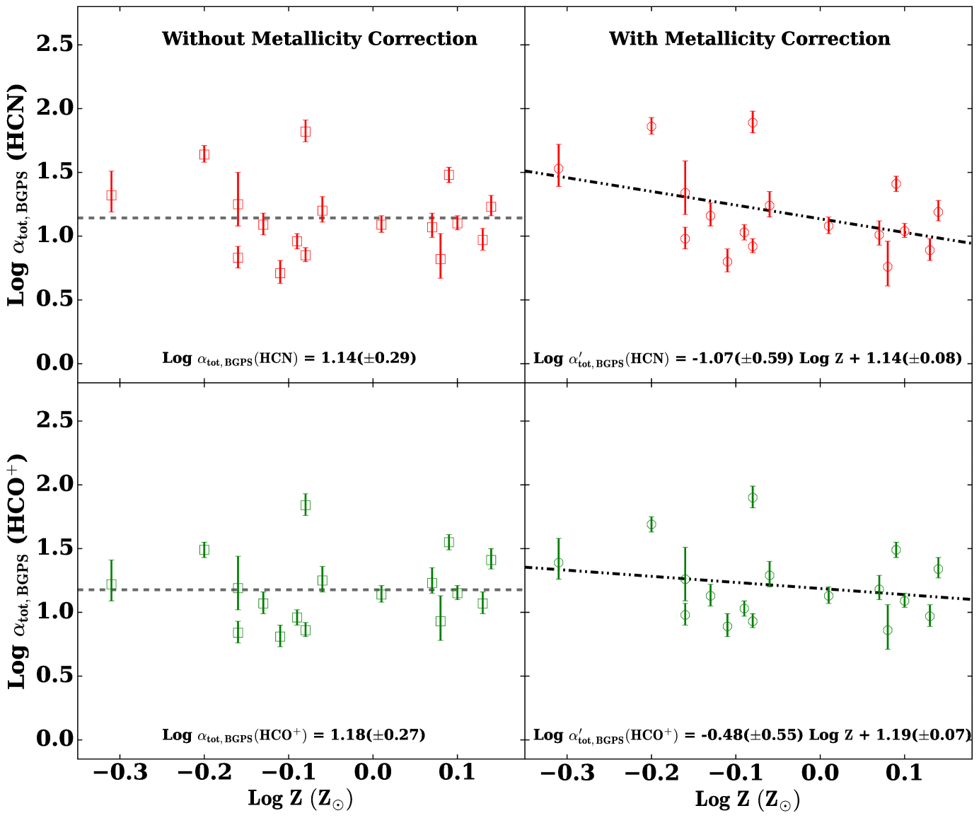
Figure 8: Variation of $\alpha_{\rm tot,BGPS}$ for HCN (top panels) and HCO⁺ (bottom panels) derived from dust based analysis with metallicity, both with (right) and without (left) metallicity correction. The horizontal dashed line in the top and bottom left panels shows the mean value of $\alpha_{\rm tot,BGPS}$. The dash-dotted line in the top and bottom right panels are done by fitting.

4.2.3 Mass Conversion factor: The alpha-factor ($\alpha_{Q}$) from Dust-based analysis

Following Section 4.1.4, we have derived mass conversion factor $\alpha_{\rm in,BGPS}$ by dividing the mass of dense gas ($M_{\rm{dg,BGPS}}$) by the HCN or HCO⁺ luminosity within the “dense” region defined by BGPS mask region. For $\alpha_{\rm tot,BGPS}$, we divide $M_{\rm{dg,BGPS}}$ by $L_{\rm tot}$ for HCN or HCO⁺. The values, presented in Table 6, are listed in logarithmic scale without metallicity correction for both HCN and HCO⁺.

Subsequently, we computed metallicity-corrected mass conversion factors $\alpha^{\prime}_{\rm in,BGPS}$ and $\alpha^{\prime}_{\rm tot,BGPS}$ for all targets in Table 7 using the metallicity-corrected dense gas mass ($M_{\rm dg,BGPS}^{{}^{\prime}}$) values. Finally, we obtained the statistical parameters separately for inner and outer Galaxy clouds, detailed in Table 8, to discern potential variations between the inner and outer Galaxy regions. Correction for the effects of metallicity leads to significant differences in $\alpha^{\prime}_{\rm tot,BGPS}$. For instance, the mean value of the $\alpha_{\rm tot,BGPS}(\mbox{{\rm HCN}})$ in linear scale is 11 and 15.5 $\mbox{M${}_{\odot}$}\ (\rm K\ km\ s^{-1}\ pc^{2})^{-1}$ for inner and outer Galaxy targets, respectively, for the case where we do not consider the metallicity correction. The $\alpha^{\prime}_{\rm tot,BGPS}$ for HCN  decreases by a factor of 1.15 for inner Galaxy clouds and increases by a factor of 1.20 for outer Galaxy targets once the correction is applied. In Figure 8, we have plotted the $\alpha_{\rm tot,BGPS}\ \rm(and\ \alpha^{\prime}_{\rm tot,BGPS})$ with respect to metallicity for both HCN and HCO⁺. These plots also show the inverse relation between mass conversion factor and metallicity.

Table 8: Statistical summary: average mass-luminosity conversion factors from BGPS analysis

		$\rm Log\ \alpha_{\rm in,BGPS}$		$\rm Log\ \alpha_{\rm tot,BGPS}$			$\rm Log\ \alpha^{\prime}_{\rm in,BGPS}$		$\rm Log\ \alpha^{\prime}_{\rm tot,BGPS}$
	HCN
Inner Galaxy		$1.61\pm 0.28$		$1.04\pm 0.15$			$1.50\pm 0.29$		$0.98\pm 0.16$
Outer Galaxy		$1.52\pm 0.27$		$1.19\pm 0.34$			$1.63\pm 0.29$		$1.27\pm 0.35$
	HCO+
Inner Galaxy		$1.65\pm 0.25$		$1.16\pm 0.18$			$1.55\pm 0.25$		$1.09\pm 0.18$
Outer Galaxy		$1.54\pm 0.27$		$1.18\pm 0.31$			$1.65\pm 0.27$		$1.26\pm 0.31$

Note. — 1. Units of conversion factors are $\mbox{M${}_{\odot}$}\ (\rm K\ km\ s^{-1}\ pc^{2})^{-1}$.

5 Mass-Luminosity conversion factors in the Solar neighborhood

In order to comprehensively assess the mass-conversion factor across the Milky Way, we included molecular clouds within the Solar neighborhood in our analysis. Several recent studies have focused on elucidating the characteristics of the nearby clouds. For instance, Dame & Lada (2023) surveyed the entire Perseus molecular cloud using the CfA 1.2m telescope, focusing on HCN. Santa-Maria et al. (2023) employed the IRAM 30m telescope to investigate the Orion B Giant Molecular Cloud (GMC). Tafalla et al. (2023) expanded their research to cover three distinct star-forming regions — California, Perseus, and Orion A – employing the IRAM 30m telescope at a wavelength of 3 mm. Yun et al. (2021, 2024), utilizing the TRAO 14m telescope, explored Orion A and Ophiuchus, concentrating on HCN and HCO⁺. We have compiled the mass and luminosity information for these clouds from the respective studies and tabulated the data in Table 9. For Ophiuchus, we extracted mass information from Evans et al. (2014) and rescaled it to the updated distance value of 137 pc. Luminosity values for HCN and HCO⁺ were obtained from Yun et al. (2024), and we subsequently calculated the total mass-to-luminosity ratio ($\mathrm{\alpha_{tot}}$). The Orion A cloud was investigated by both Tafalla et al. (2023) and Yun et al. (2021, 2024). The luminosity values in the corrected table (Yun et al., 2024) are consistent with those in Tafalla et al. (2023). However, Yun et al. (2021) did not measure the dense-gas mass, so we have used the mass information from Tafalla et al. (2023). Similarly, the Perseus molecular cloud was studied by Tafalla et al. (2023) and Dame & Lada (2023). Both studies indicate higher $\mathrm{\alpha_{tot}}$ values for Perseus compared to most clouds, excluding Ophiuchus. The $\mathrm{\alpha_{tot}(\mbox{{\rm HCN}})}$ value reported by Dame & Lada (2023) is significantly larger than that of Tafalla et al. (2023). The observed discrepancy in values may be attributed to differences in the methodology employed for calculating HCN luminosity. Dame & Lada (2023) mentioned that $\mathrm{\alpha_{tot}(\mbox{{\rm HCN}})=76\ \mbox{M${}_{\odot}$}\ (\rm K\ km\ s^{-1}\ pc^{2})^{-1}}$ if they consider HCN outside their sampling boundary, which is consistent with Tafalla et al. (2023).

Across the entire sample of Solar neighborhood clouds, the dense-gas mass to HCN luminosity for the entire cloud varies from 23 to 122 $\mbox{M${}_{\odot}$}\ (\rm K\ km\ s^{-1}\ pc^{2})^{-1}$. The $\mathrm{\alpha_{tot}}$ values for HCN and HCO⁺ for the Perseus and Ophiuchus clouds are notably higher than the typical values. In Figure 7, we have indicated the $\alpha_{\rm tot}$ values of individual local clouds with the blue star marks. The local clouds are not shown in Figure 8 because BGPS surveys of nearby clouds were sensitive only to cores, not the larger clumps (Dunham et al., 2011).

Most of the values of $\mathrm{\alpha_{tot}}$ are notably higher for the Solar neighborhood clouds, especially the low-mass clouds, Perseus and Ophiuchus. We have computed the average values, both with and without those two clouds, in Table 9. Translated to actual values, the average without the two clouds is about 50% bigger than our fitted relationship would predict. With those two clouds, the average is about three times larger. Neither of those two clouds is characteristic of the clouds in our sample, so the conversion factors may be affected by other properties.

Table 9: Dense gas masses and conversion factors in molecular clouds from the Solar neighborhood

Cloud	Log $M_{\rm dense}$	Log $L_{\rm tot}$	Log $\mathrm{\alpha_{tot}}$	Log $L_{\rm tot}$	Log $\mathrm{\alpha_{tot}}$	References
	M⊙	HCN	HCN	HCO+	HCO+
California	3.68	2.32	1.36	2.24	1.45	Tafalla et al. (2023)
Orion B	3.49	2.04	1.46	2.08	1.40	Santa-Maria et al. (2023)
Orion A	4.38	2.72	1.66	2.73	1.64	Tafalla et al. (2023)
	4.38	2.62	1.76	2.61	1.76	Yun et al. (2021, 2024), Tafalla et al. (2023)
Ophiuchus	3.16	1.08	2.09	1.03	2.13	Yun et al. (2021, 2024), Evans et al. (2014)
Perseus	3.75	1.89	1.86	1.91	1.83	Tafalla et al. (2023)
	3.71	1.74	1.96	$\cdots$	$\cdots$	Dame & Lada (2023)
Mean	3.69	1.98	1.71	1.99	1.70
Median	3.68	2.04	1.71	2.08	1.70
Std	0.45	0.60	0.30	0.60	0.30
Mean†	3.85	2.34	1.51	2.33	1.52
Median†	3.68	2.32	1.46	2.24	1.45
Std†	0.47	0.31	0.18	0.30	0.16

Note. — 1. Units of luminosities are K km s^-1pc².

2. Units of conversion factors are $\mbox{M${}_{\odot}$}\ (\rm K\ km\ s^{-1}\ pc^{2})^{-1}$.

3. ^†We have excluded Ophiuchus and Perseus from the statistical analysis of these local clouds.

6 Discussion

6.1 Effect of Metallicity on Mass Conversion Factor

The outer Milky Way is a convenient proxy for other low-metallicity systems, at the same time offering easier and clearer observations of molecular clouds than nearby galaxies. This study explores the impact of metallicity on the mass-luminosity conversion factor of dense gas in the Milky Way, comparing the inner parts of the Galaxy, with metallicity up to 1.29 times solar metallicity, with the outer disk, where the metallicity falls as low as 0.3 times the solar metallicity.

Recent studies (Shimajiri et al., 2017; Kauffmann et al., 2017; Pety et al., 2017; Evans et al., 2020; Barnes et al., 2020; Patra et al., 2022; Dame & Lada, 2023; Tafalla et al., 2023; Santa-Maria et al., 2023) have highlighted that HCN, HCO⁺ emissions can originate from regions with low levels of extinction and emphasized the need to account for the entire cloud when calculating the $\alpha_{Q}$ factor for comparison with extra-galactic studies, where the line luminosity of the whole cloud is used to estimate mass. Gao & Solomon (2004b) estimated the value for the extragalactic conversion factor $\alpha_{\rm HCN(1\to 0)}=10$ $\mbox{M${}_{\odot}$}\ (\rm K\ km\ s^{-1}\ pc^{2})^{-1}$ from a theoretical consideration, where luminosity from the whole cloud is considered to obtain mass. This value has been widely adopted, although Neumann et al. (2023) use a value of 14, rather than 10. In the following section, we discuss the effect of metallicity on mass conversion factor when the line luminosity is computed from the whole cloud ($\alpha_{\rm tot}$), which is most relevant to extragalactic comparisons.

In Section 4.1.4, we calculated $\alpha_{\rm tot,Gas}$ and $\alpha^{\prime}_{\rm tot,Gas}$ for HCN and HCO⁺ from a gas-based analysis, without and with metallicity correction, respectively. Figure 7 presents all the results in a four-panel diagram. The upper left and lower left panels of Figure 7 illustrate $\mathrm{log\ \alpha_{\rm tot,Gas}}$ plotted against $\mathrm{log\ Z}$ for HCN and HCO⁺, respectively, without accounting for metallicity corrections in the analysis. All data points scatter around the mean value, represented by the black dashed line, revealing a ‘flat’ distribution without significant upward or downward trends. It corresponds to a constant mass-luminosity conversion factor across the Galaxy when metallicity corrections are not considered. The mean value of the logarithm translates to $\mathrm{\alpha_{\rm tot,Gas}}$ for HCN of $22.9^{+26.1}_{-12.2}$ $\mbox{M${}_{\odot}$}\ (\rm K\ km\ s^{-1}\ pc^{2})^{-1}$; for HCO⁺, the value is $23.4^{+26.7}_{-12.5}$ $\mbox{M${}_{\odot}$}\ (\rm K\ km\ s^{-1}\ pc^{2})^{-1}$, combining both inner and outer Galaxy clouds. These values are around a factor of 2 higher than the value derived by Gao & Solomon (2004a), and commonly used in extragalactic studies. We have also plotted the $\alpha_{\rm tot}$ values of the local clouds mentioned in Table 9 in Figure 7.

The scenario changes when we use the metallicity correction in the analysis outlined in section 4.1. The targets with low metallicity (i.e., with large $R_{\rm G}$) show higher $\mathrm{\alpha^{\prime}_{\rm tot,Gas}}$ value compared the targets with higher metallicity (or located in the inner Galaxy). The upper right and lower right panels of Figure 7 illustrate $\mathrm{log\ \alpha^{\prime}_{\rm tot,Gas}}$ plotted against $\mathrm{log}\ Z$ for HCN and HCO⁺, respectively, after considering the metallicity corrections in the analysis. Both HCN and HCO⁺ conversion factors demonstrate a decreasing trend with increasing metallicity, echoing the observed pattern in $\mathrm{X_{CO}}$ variation with metallicity (Gong et al., 2020; Lee et al., 2024). The Pearson correlation parameter between $\mathrm{\alpha^{\prime}_{tot,gas}(\mbox{{\rm HCN}})}$ and $\mathrm{log}\ Z$, the Pearson correlation coefficient is $-0.53$, and for HCO⁺ it is $-0.51$ (see Figure 11). To quantitatively analyze this relationship, we fit linear functions in log-log space to derive the scaling relations. However, we have not included the local clouds for the fitting because of the diversity of mass measurements and the outer boundary definitions. For HCN, the scaling relation obtained from this dataset is $\mathrm{\alpha^{\prime}_{tot,gas}(\mbox{{\rm HCN}})\propto Z^{-1.53(\pm 0.59)}}$ and for HCO⁺, it is $\mathrm{\alpha^{\prime}_{tot,gas}(\mbox{{\rm HCO}${}^{+}$})\propto Z^{-1.32(\pm 0.55)}}$. While uncertain, the $Z$ dependence for HCN is stronger than linear; this would be consistent with the evidence for strong dependence of the HCN abundance on metallicity (Shimonishi, 2024). Similarly in section 4.2.3, we have calculated the mass-luminosity conversion factor $\alpha_{\rm tot,BGPS}$ by taking the ratio between the dense mass of gas obtained from BGPS dust continuum data and HCN, HCO⁺ line luminosities from the entire cloud. The upper left and lower left panels of Figure 8 illustrate $\mathrm{log\ \alpha_{\rm tot,BGPS}}$ plotted against $\mathrm{log}\ Z$ for HCN and HCO⁺, respectively, without accounting for metallicity corrections in the analysis. The black-dashed lines correspond to the mean value of $\alpha_{\rm tot,BGPS}$ in logarithmic scale, combining inner and outer Galaxy targets. The mean values, converted from the logarithm, are $\mathrm{\alpha_{\rm tot,BGPS}}$ for HCN $13.8^{+13.1}_{-6.7}$ $\mbox{M${}_{\odot}$}\ (\rm K\ km\ s^{-1}\ pc^{2})^{-1}$ and for HCO⁺, $15.1^{+13.0}_{-7.0}$ $\mbox{M${}_{\odot}$}\ (\rm K\ km\ s^{-1}\ pc^{2})^{-1}$, combining both inner and outer Galaxy clouds.

The upper and lower right panels of Figure 8 depict the variation of $\mathrm{log\ \alpha^{\prime}_{\rm tot,BGPS}}$ with $\mathrm{log}\ Z$ for HCN and HCO⁺, respectively, after correcting for the metallicity in the dense gas mass obtained from dust continuum data. The conversion factor for HCN shows an decreasing trend with increasing metallicity, while for HCO⁺ the trend is weak. To quantify the analysis, we fitted the data as shown in the figures and the scaling relations are $\mathrm{\alpha^{\prime}_{tot,BGPS}(\mbox{{\rm HCN}})}\propto Z^{-1.07(\pm 0.59)}$ for HCN, and $\mathrm{\alpha^{\prime}_{tot,BGPS}(\mbox{{\rm HCO}${}^{+}$})}\propto Z^{-0.48(\pm 0.55)}$ for HCO⁺. The Pearson correlation parameter between $\mathrm{\alpha^{\prime}_{tot,BGPS}(\mbox{{\rm HCN}})}$ and $\mathrm{log}\ Z$ is $-0.47$ and for HCO⁺ it is $-0.28$, respectively.

The mass conversion factors derived from the gas-based analysis in Section 4.1 are somewhat higher than those from the BGPS-based analysis in Section 4.2. This difference is caused by the fact that $M_{\rm dg,Gas}$ is on average higher than $M_{\rm dg,BGPS}$ (mean ratio is 1.76, with a median value of 1.54 and a standard deviation of 1.64, indicating substantial dispersion). This fact seems in conflict with Figure 1, which shows that the BGPS (cyan) contours are bigger than the gas-based dense regions (white (or red) contours) for most (but not all) of the clouds (e.g., Sh2-132, Sh2-142, Sh2-242, Sh2-266, Sh2-269). Comparison with the $N_{\rm H_{2}}$ maps indicates that BGPS mask boundaries correspond to regions with $A_{\rm V}$ values ranging from 3-8 magnitudes across the sample, so that the BGPS traces somewhat lower density regions on average, and thus should result in larger masses. The discrepancy is probably caused by the assumed opacity at 1.1 mm, which may be too high for these regions.

Despite these caveats, both analyses show that using the traditional method without correcting for metallicity in galactic clouds results in overestimating the mass conversion factor (and therefore the mass) for entire clouds in the inner part of the Galaxy (or high metallicity regions). Simultaneously, it leads to underestimating the mass conversion factor (and thus the mass) in outer Galaxy regions (or low metallicity regions).

Without correcting for metallicity effects, no variations in the mass conversion factors with $Z$ are seen (left panels of Figures 7 and 8). Linear fits to those data showed no statistically significant slopes: $0.05\pm 0.59$, $0.32\pm 0.60$, $-0.37\pm 0.58$, $0.19\pm 0.54$ for $\alpha_{\rm tot,Gas}$(HCN), $\alpha_{\rm tot,Gas}$(HCO⁺), $\alpha_{\rm tot,BGPS}$(HCN), $\alpha_{\rm tot,BGPS}$(HCO⁺), respectively. The most significant of these is 0.6 of the uncertainty on the slope and most are much smaller than the uncertainty. Because the mass is measured with ¹³CO or dust emission, both assumed to scale with metallicity, the most likely explanation is that the HCN and HCO⁺ emission also scales with metallicity, thus cancelling out. In the left panels, no scaling of mass determined from ¹³CO or dust with $Z$ is applied, so masses at $Z>1$ are overestimated by the factor, $Z$. If HCN and HCO⁺ emission increases linearly with $Z$, the luminosities will increase in the same way, obscuring any actual trend in $\alpha_{\rm tot}$. We find dependences on $Z$ that are somewhat stronger than linearly proportional, but linear with uncertainties. Our model for how the mass depends on $Z$ is very simple, indicating the need for theoretical analysis for the $Z$ dependence of HCN and HCO⁺ emission, similar to that available for CO (Gong et al., 2020; Hu et al., 2022).

While our main focus is on $\alpha_{\rm tot}$, relevant to extra-galactic studies, we comment briefly on $\alpha_{\rm in}$ relevant to studies in the Milky Way. Wu et al. (2010) was the first to attempt to obtain $\alpha_{\text{in}}(\text{HCN})$ for massive, dense cores in the Milky Way, which was found to be on average 20 $\mbox{M${}_{\odot}$}\ (\rm K\ km\ s^{-1}\ pc^{2})^{-1}$. Shimajiri et al. (2017) calculated $\alpha_{\text{in}}(\text{HCN})$ in the range of $35–454$ for 10 heavily extincted regions with $\mbox{$A_{\rm V}$}>8$ mag based on Herschel dust map, indicating a large spread in the derived values.

Without correcting for metallicity, the average values, converted from logarithmic to linear scale, for the mass conversion factor in the dense region are 78 and 76 $\mbox{M${}_{\odot}$}\ (\rm K\ km\ s^{-1}\ pc^{2})^{-1}$ for inner and outer Galaxy targets, respectively, in gas-based analysis (mentioned in Section 4.1.4). However, after applying the metallicity correction, the mean values in linear scale decreases to 63 $\mbox{M${}_{\odot}$}\ (\rm K\ km\ s^{-1}\ pc^{2})^{-1}$ for inner Galaxy targets and increases to 117.5 $\mbox{M${}_{\odot}$}\ (\rm K\ km\ s^{-1}\ pc^{2})^{-1}$ for outer Galaxy targets, respectively. The same trend is observed for HCO⁺. Also, in the analysis based on BGPS, the mass conversion factor ($\alpha_{\text{in}}(\mbox{{\rm HCN}})$) derived from the dense regions of the cloud decreases by a factor of 1.29 for inner Galaxy clouds, whereas for outer Galaxy targets, it increases by the same factor, after applying the metallicity correction. The high value of $\alpha_{\text{in}}$ observed in our study, as well as in the local clouds discussed in Section 5 can be explained by the larger mapping area conducted in these cases compared to that of Wu et al. (2010). The latter primarily focused on the clump positions within the dense regions of the cloud rather than encompassing the entire area.

For maps of resolved regions, common in Galactic studies, the observational details, such as sensitivity and mapping area have a major impact on the conversion from observations to the mass of dense gas.

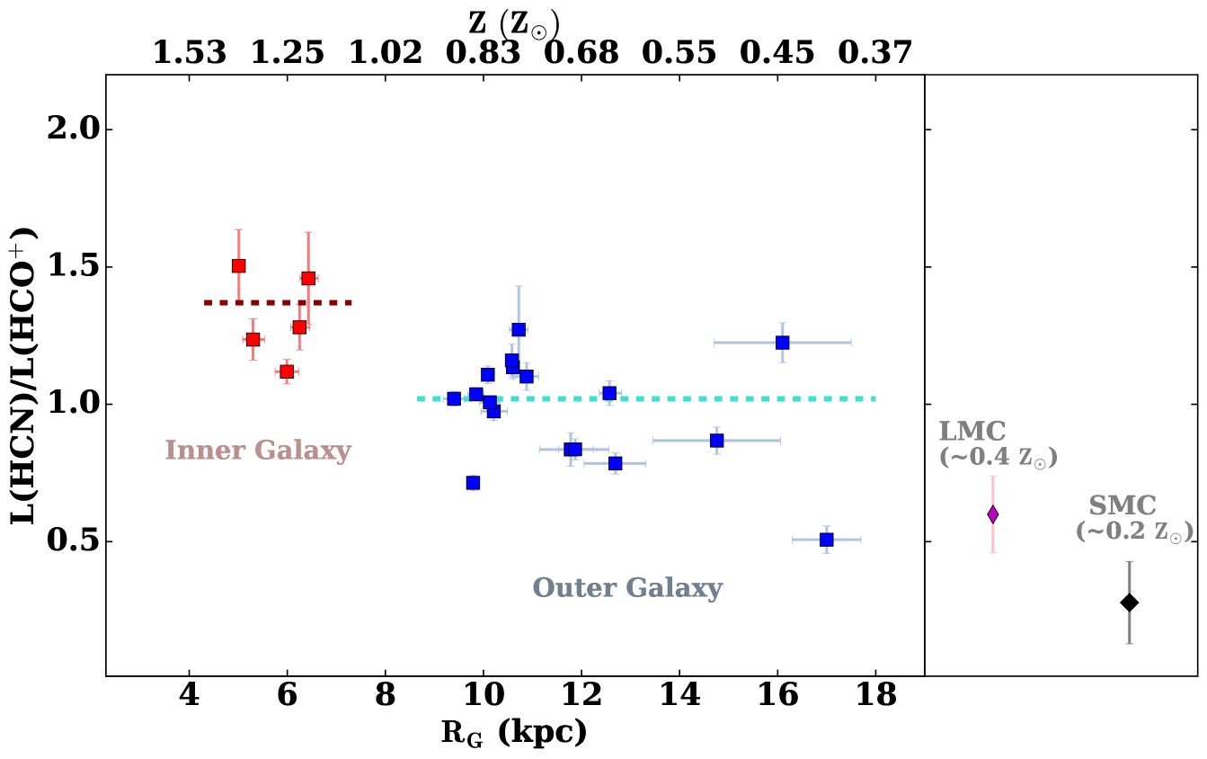
Figure 9: Luminosity ratio of HCN and HCO⁺ for inner Galaxy (red squares) and outer Galaxy (blue squares) targets, as a function of $R_{\rm G}$. The red and cyan dashed line show the median value of $L(\mbox{{\rm HCN}})/L(\mbox{{\rm HCO}${}^{+}$})$ for the inner and outer Galaxy sample, respectively. The magenta and black diamonds show the HCN and HCO⁺ ratio for LMC, SMC (Chin et al., 1997; Galametz et al., 2020), respectively.

6.1.1 Comparison between HCN and HCO⁺ as tracers

The bottom right panel of Figure 8 shows that the luminosity to mass conversion for HCO⁺ is less sensitive to metallicity than the same factor for HCN, making it more robust against metallicity variations. HCN and HCO⁺ are both linear molecules, with similar dipole moments, but the collisional cross-section of HCO⁺ is significantly larger than that of HCN. The net result is that the effective density for excitation of the $J=1\rightarrow 0$ transition of HCO⁺ is about 0.12 that for HCN (Shirley, 2015), suggesting that HCN would better probe the denser gas. However, other factors like radiative trapping and other excitation mechanisms such as electron collisions and mid-infrared pumping also affect the line luminosity. Chemical abundances can also affect the observed luminosities. The substitution of $\rm O^{+}$ for N in HCO⁺ suggests that the nitrogen-to-oxygen (N/O) abundance ratio will affect the relative abundance of these molecules. Pineda et al. (2024) finds a steeper dependence on $R_{\rm G}$ for N/H ($-0.068$ dex/kpc) than the dependence for O/H ($-0.044$ dex/kpc).

These molecules have been observed also in low-metallicity galaxies (Chin et al., 1997; Buchbender et al., 2013; Braine et al., 2017; Galametz et al., 2020). The previous studies on LMC, SMC, M33, IC10, M31 show that the $\mbox{{\rm HCN}}/\mbox{{\rm HCO}${}^{+}$}$ intensity ratio decreases from solar to sub-solar metallicity galaxies. Further decreases have been observed in the Large Magellanic Cloud, where the ratio is approximately 0.6 (Chin et al., 1997), and in the Small Magellanic Cloud, where it reaches 0.3 (Chin et al., 1998).

In Figure 9, we have plotted the luminosity ratio of HCN and HCO⁺  ($L_{\mathrm{tot}}(\mbox{{\rm HCN}})/L_{\mathrm{tot}}(\mbox{{\rm HCO}${}^{+}$})$) for the entire sample including five inner Galaxy and 17 outer Galaxy targets. It shows that $L_{\mathrm{tot}}(\mbox{{\rm HCN}})/L_{\mathrm{tot}}(\mbox{{\rm HCO}${}^{+}$})$ decreases with increasing $R_{\rm G}$. The median value of $L_{\mathrm{tot}}(\mbox{{\rm HCN}})/L_{\mathrm{tot}}(\mbox{{\rm HCO}${}^{+}$})$ is 1.37 for the inner Galaxy targets and 1.02 for the outer Galaxy sample. For comparison, the LMC and SMC are also shown on the right. The $L(\mbox{{\rm HCN}})/L(\mbox{{\rm HCO}${}^{+}$})$ ratios for the two nearest low-metallicity dwarf galaxies are marked with magenta and black diamond points (Chin et al., 1997; Galametz et al., 2020), highlighting the trend of decreasing ratio with lower metallicity. In other words, the luminosity ratio of $\mbox{{\rm HCN}}/\mbox{{\rm HCO}${}^{+}$}$ decreases by a factor of 3 as the metallicity decreases from 1.3 $\rm Z_{\odot}$ to 0.3 $\rm Z_{\odot}$, in agreement with Braine et al. (2017). This behavior is consistent with a strong change in the abundance ratio of HCO⁺ to HCN with $Z$ and with [N/H] in particular (Shimonishi, 2024; Nishimura et al., 2016a, b).

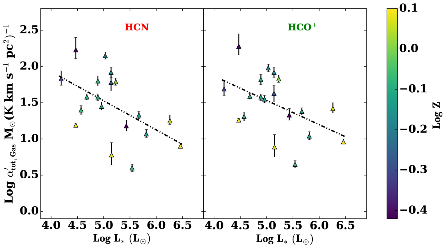
Figure 10: Variation of $\alpha_{\rm tot,Gas}$ derived from gas based analysis with bolometric luminosity from nearby massive star(s) and the metallicity of the regions.

6.2 Dispersion in the dense gas mass conversion factor

The dispersion in the $\alpha_{\rm tot}$ values across different regions is quite large, even after applying the metallicity correction. We consider here the possible effects of radiation, as traced by the total stellar luminosity of the associated cluster. The ultraviolet (UV) radiation from the massive stars (OB type stars) impacts the physics and chemistry of star-forming regions significantly. Shimajiri et al. (2017) mentioned that the the conversion factors for HCN and HCO⁺ anti-correlate with the strength of the local UV radiation. Mirocha et al. (2021) also studied the impact of UV on HCN in the immediate surroundings of protostars, but they did not find much effect of UV on the overall HCN. Pety et al. (2017) showed that the molecules such as HCN (also HCO⁺, CN, and HNC) are sensitive to the far-UV radiation produced from star formation. In short, the effect of UV on $\alpha_{\rm tot}$ has been unclear.

We have used the $\alpha_{\rm tot}$ value obtained from gas-based analysis since all the targets are included. For instance, Sh2-270 and Sh2-209 both are metal-poor star forming regions with 12+log[O/H] value 8.08 and 8.09, respectively. Despite their similarity in metallicity, the $\alpha_{\rm tot}$ values for these regions exhibit a huge difference. The $\alpha_{\rm tot}(\mbox{{\rm HCN}})$ value for Sh2-209 is 15 $\mbox{M${}_{\odot}$}\ (\rm K\ km\ s^{-1}\ pc^{2})^{-1}$, whereas $\alpha_{\rm tot}(\mbox{{\rm HCN}})$ for Sh2-270 is 11 times higher than Sh2-209, 170 $\mbox{M${}_{\odot}$}\ (\rm K\ km\ s^{-1}\ pc^{2})^{-1}$. The difference in the number of massive stars among these regions is striking; Sh2-270 has only one B-type star (Méndez-Delgado et al., 2022), whereas Sh2-209 has at least 4 O-type and 1 B-type star (Yasui et al., 2023). This difference in the number of massive stars suggests a stronger far-ultraviolet (UV) radiation field in Sh2-209, as O-type stars are known to emit significant amounts of UV radiation. The UV radiation is 9 times stronger in Sh2-209 region compared to Sh2-270. The UV can help with excitation by creating photo-ionization, and electrons excite the HCN (Goldsmith & Kauffmann, 2017); as a result $\alpha_{\rm tot}$ will be lower for regions having a strong UV radiation field. We have seen a similar case for another pair of regions — Sh2-142 and Sh2-235 ($\mathrm{12+log[O/H]\sim 8.43}$); Sh2-142 has binary O-type stars DH Cep (O6$+$O7) (Sharma et al., 2022); Sh2-235 has a single O-type (O9.5V) star and a few B-type stars (Kirsanova et al., 2008). While both clouds have O stars, the early type binary will produce a lot more ionizing photons than one O9.5 star, resulting in Sh2-142 having seven times stronger UV radiation compared to the Sh2-235 region. In this case, Sh2-142 has low $\alpha_{\rm tot}$ compared to Sh2-235. Among the solar neighborhood star forming regions, Perseus and Ophiuchus have very large $\alpha_{\rm tot}$ values for HCN and HCO⁺. These regions lack OB stars, thereby avoiding the influence of UV radiation emitted by such massive stars. Consequently, the dominance of electrons for the excitation of HCN is not significant in these areas, resulting in high $\alpha_{\rm tot}$ values for HCN. Santa-Maria et al. (2023) argue that the enhanced UV radiation favors the formation of HCN and the excitation of the $J=1-0$ line at large scales for Orion B.

Because we lack information on the UV radiation for some regions, we use the total stellar luminosity ($L_{*}$) as a proxy for external radiation, as reported in Table 1. For the outer Galaxy clouds, we have used the spectral types of the main stars (spectral types earlier than B2) from Méndez-Delgado et al. (2022) or from the literature on the cluster. From these, we computed the bolometric luminosity for each region from Binder & Povich (2018). We have no direct information on the stars for the inner Galaxy targets, so we assume that $L_{*}$ is the same as the far-infrared luminosity ($L_{\mathrm{FIR}}$). $L_{\mathrm{FIR}}$ was derived by combining data from the MIPSGAL (Spitzer) and Hi-GAL (Herschel) surveys, covering wavelengths from 24 to 500 $\mu$m. A spectral energy distribution (SED) was constructed for each pixel, and its integral was calculated. As a first step, all maps were re-projected onto a common grid corresponding to the coarsest resolution, that of the Herschel 500 $\mu$m map. For each pixel, a modified blackbody function was fitted to the portion of the SED at wavelengths $\lambda\geq 160\mu$m (e.g., Elia et al., 2013). The total SED integral was then calculated by summing two components: the integral of the observed SED between 24 and 160 $\mu$m and the analytic integral of the best-fit modified blackbody for $\lambda\geq 160\mu$m, an extrapolation that adds the contribution from unmapped emission at $\lambda>500\mu$m. After appropriate unit conversions, the final pixel luminosity was obtained by multiplying by the factor $4\pi D^{2}$, where $D$ is the heliocentric distance. Finally, the luminosities of all pixels lying within the defined outer boundary ($N_{\rm{H_{2}}}^{{}^{\prime}}\geq 1.5\times 10^{21}\ \rm{cm^{-2}}$) were summed to obtain the total luminosity of the region.

In Figure 10, we plot the $\mathrm{log}\ \alpha^{\prime}_{\rm tot,Gas}$ against the total bolometric luminosity ($\mathrm{log}\ L_{*}$) of nearby massive stars. The color gradient in the plot represents the variation in metallicity values. The regions with higher metallicity (i.e., the points with yellowish color) show higher bolometric luminosity (Urquhart et al., 2024). Regions exhibiting higher radiation levels display lower $\alpha^{\prime}_{\rm tot}$ values compared to clouds with comparable metallicity levels. We have calculated the correlation parameter between $\mathrm{\alpha^{\prime}_{\rm tot,Gas}(\mbox{{\rm HCN}})}$ and $\mathrm{log}\ L_{*}$; the Pearson correlation coefficient is $-0.54$ and for HCO⁺ it is $-0.49$ (Figure 11). The fit to the relation between $\alpha^{{}^{\prime}}_{\rm tot,Gas}(\rm HCN)$ and $\rm log\ L_{*}$ is (in linear scale and normalized to a typical luminosity) $\alpha^{{}^{\prime}}_{\rm tot,Gas}(\rm HCN)=33.6(L_{*}/10^{5})^{-0.40\pm 0.15}$. For HCO⁺, the relation is $\alpha^{{}^{\prime}}_{\rm tot,Gas}(\rm\mbox{{\rm HCO}${}^{+}$})=34.0(L_{*}/10^{5})^{-0.33\pm 0.14}$. These relations are valid only for the range of $\mathrm{log}\ L_{*}$ in this sample.

6.3 Multiple Factors affecting the mass conversion factors

In Figures 7 and 8, the mass conversion factor varies with metallicity for both HCN and HCO⁺, though HCO⁺ exhibits a weaker dependence on metallicity. Another contributor to the scatter in the plot is the variation in UV field strength, as illustrated in Figure 10. In Figure 11, we have shown the correlation matrix, which is a $5\times 5$ square matrix with the same variables shown in the rows and columns. This correlation matrix represents how different variables ($\alpha^{\prime}_{\rm tot,Gas}(\mbox{{\rm HCN}})$, $\alpha^{\prime}_{\rm tot,Gas}(\mbox{{\rm HCO}${}^{+}$})$, $\mathrm{log}\ Z\mathrm{(Z_{\odot}})$, $R_{\rm G}$, and $\textrm{ log}\ L_{*}$) interact with each other. In the correlation matrix, the Pearson correlation coefficient is calculated between pairs of variables, considering only the two variables at a time and disregarding the contribution of other variables. Figure 11 reveals that $\alpha^{\prime}_{\rm tot,Gas}(\text{HCN})$ and $\alpha^{\prime}_{\rm tot,Gas}(\text{HCO}^{+})$ exhibit a moderate negative correlation with both metallicity and the bolometric luminosity from external radiation. It is noteworthy that the $\alpha^{\prime}_{\rm tot}$ values for HCN and HCO⁺ are equally influenced by metallicity and UV radiation from massive stars.

There could be several other potential factors that can influence the mass conversion factors. For example, the evolutionary stages of the regions may be different. The evolutionary stage affects the gas distribution, radiation field, and star formation feedback processes, which in turn influence both the mass of the region and its luminosity, thus altering the mass-to-luminosity conversion factor over time. There can be other factors like the dust grain properties or the cosmic ray ionization rate in the region. Though these factors are potentially important, our current dataset is limited in scope and does not allow for a full exploration of these variables. This presents an exciting opportunity for future work to investigate these influences in greater detail. In particular, observing more sources in the inner Galaxy with metallicity and well sampled maps of HCN and HCO⁺  is the most pressing need.

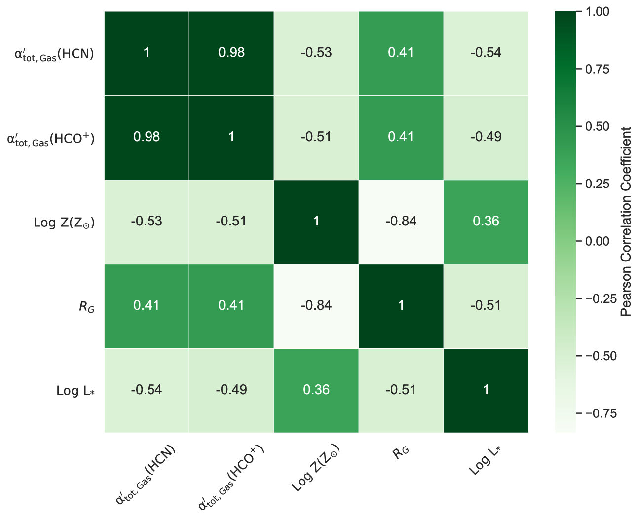
Figure 11: The Correlation Matrix: Correlation among the parameters $\alpha_{\rm tot,Gas}(\mbox{{\rm HCN}})$, $\alpha_{\rm tot,Gas}(\mbox{{\rm HCO}${}^{+}$})$, $\mathrm{Log}\ Z\mathrm{(Z_{\odot}})$, $R_{\rm G}$, and $\mathrm{Log}\ L_{*}$. The color scale represents the Pearson correlation coefficient, as indicated by the labeled color bar.

6.4 Impact of Metallicity on Dense Gas Mass in the Central Molecular Zone

A longstanding puzzle in astronomy is the slow rate of star formation per unit mass of dense gas in the Central Molecular Zone (CMZ) of the Milky Way (Longmore et al., 2013). While there are many factors that may be at work (see Henshaw et al. 2023 for a recent review), essentially all measures of dense gas mass (molecular line emission, dust continuum emission, etc.) are likely to be affected by metallicity. Extrapolating the relations of Méndez-Delgado et al. (2022) to $\mbox{$R_{\rm G}$}=0.5$ kpc predicts $Z=2.18$. If we extrapolate our scaling relation for HCN to the CMZ, $\alpha^{\prime}_{\rm tot,Gas}(\mbox{{\rm HCN}})=5.92$, and $\alpha^{\prime}_{\rm tot,BGPS}(\mbox{{\rm HCN}})=5.99$, about 1/3 the local values. The nitrogen abundance in the CMZ is about 1.3 times higher than the local value (Pineda et al., 2024). If this factor increases the NH₃ abundance used by Longmore et al. (2013) to estimate dense gas mass, it would decrease the dense gas mass estimate. Similarly, Ginsburg et al. (2018) used a $\gamma$ of 100 to compute surface densities from Herschel data for Sgr B2, concluding that the threshold surface density for star formation is at least an order of magnitude larger than the local value. If $\gamma$ ratio varies according to equation 15, the column density estimates would decrease by a factor of about 2. The same would be true for the CMZoom study (Battersby et al., 2020) and the recent analysis of 3D-CMZ (Battersby et al., 2024), which also assumed $\gamma=100$. Interestingly, Elia et al. (2025) found no deficit of star formation in the CMZ compared to that predicted from dense gas relations using the Hi-GAL catalog of dense clumps.

Consideration of the effects of metallicity on inferred cloud and clump properties in the CMZ may contribute substantially to explaining the low star formation rate per dense gas mass, along with recent evidence of higher incipient star formation rates (Hatchfield et al., 2024). The amount of dense gas may also be overestimated if molecular line conversion factors are overestimated in regions of large velocity dispersions, as seen in the centers of other barred galaxies (Teng et al., 2024).

7 Conclusions

In this study, we have analyzed 17 outer Galaxy clouds, along with 5 inner Galaxy clouds from Evans et al. (2020), and 5 local clouds to obtain a sample with metallicity range from $0.38\ \rm Z_{\odot}-1.29\ \rm Z_{\odot}$. We have investigated the impact of metallicity on the mass-luminosity conversion factor obtained from HCN and HCO⁺, commonly used tracers of dense gas.

1. The metallicity can be an important factor to consider when calculating the mass of dense gas using HCN or HCO⁺. The average value of $\alpha_{\rm tot}(\mbox{{\rm HCN}})$ is $\sim 3$ times higher in the outer Galaxy than in the inner Galaxy after correcting for metallicity.

2. We suggest to use $\alpha^{{}^{\prime}}_{\textrm{ tot, Gas}}(\textrm{HCN})=19.5^{+5.6}_{-4.4}Z^{(-1.53\pm 0.59)}$ and $\alpha^{{}^{\prime}}_{\textrm{ tot, Gas}}(\textrm{\mbox{{\rm HCO}${}^{+}$}})=21.4^{+5.5}_{-4.4}Z^{(-1.32\pm 0.55)}$ for the metallicity corrected dense gas factor for extragalactic studies.

3. Analyses of HCN emission in other galaxies (e.g., Neumann et al. 2023) may have been systematically underestimating the mass of dense gas by using smaller conversion factors in galaxies with solar metallicity. Larger factors could arise for metallicities considerably different from solar.

4. Our results indicate that HCO⁺ is less sensitive to metallicity than HCN, so HCO⁺ may be the more robust tracer of dense gas. The luminosity ratio $L(\mbox{{\rm HCN}})/L(\mbox{{\rm HCO}${}^{+}$})$ decreases by a factor of 3 as the metallicity drops from 1.3 $\rm Z_{\odot}$ to 0.3 $\rm Z_{\odot}$.

5. The dispersion in the mass conversion factors are large, even after correction for metallicity. The effect of environment, in particular UV luminosity, appears to have an effect similar in significance to that of metallicity. This effect could be important in low-$Z$ dwarf galaxies with higher radiation fields and less dust shielding.

6. The mass conversion factors derived from gas based analysis and BGPS based analysis differ. The gas-based $\alpha_{\rm tot}$ values are about 1.7 times the BGPS-based values, reflecting lower masses in the dust-based definition of dense gas. This is likely related to the choice of dust continuum opacity.

7. The values of $\alpha_{\rm tot}$ for Solar neighborhood clouds tend to be higher than predicted by our best-fitting relations, especially for the low-mass star forming regions.

8. Extrapolation of the metallicity corrections to the Central Molecular Zone would result in column densities lower than the usual estimates by factors of 2 to 3, contributing to an explanation of the relatively slow star formation there.

Appendix A TRAO Data Reduction

We follow the standard data reduction method explained in Appendix A of Patra et al. (2022). The steps are as follows. We first examine the data to identify the velocity intervals with significant emission ($v_{win}$). Next, we exclude the velocity window containing line emission and subtract the second-order polynomial baseline, utilizing only the velocity range necessary to obtain a good baseline at both ends ($v_{sp}$). We varied the velocity range ($v_{sp}$) and baseline order to achieve the best fit (for more details see Patra et al. 2022). Following this, we generate spectral cubes in FITS format to facilitate further analysis. Details regarding the total velocity range and excluded windows can be found in Table LABEL:tab:reduction.

Table 10: Velocity intervals considered for baseline subtraction and integration

Source	Line	$v_{sp}$	$v_{win}$
		(km s-1)	(km s-1)
Sh2-128	12CO	-110, -35	-80, -65
	13CO	-110, -35	-80, -65
	HCO+	-110, -35	-80, -65
	HCN	-110, -35	-85, -60
Sh2-132	12CO	-80, -10	-55, -38
	13CO	-80, -10	-55, -38
	HCO+	-80, -10	-55, -38
	HCN	-80, -10	-58, -35
Sh2-142	12CO	-75, -10	-46, -34
	13CO	-75, -10	-46, -34
	HCO+	-75, -10	-46, -34
	HCN	-75, -10	-54, -32
Sh2-148	12CO	-75, -25	-58, -44
	13CO	-75, -25	-58, -44
	HCO+	-75, -25	-58, -44
	HCN	-75, -25	-60, -42
Sh2-156	12CO	-90, -15	-60, -44
	13CO	-90, -15	-60, -44
	HCO+	-90, -15	-60, -44
	HCN	-90, -15	-65, -40
Sh2-209	HCO+	-80, -30	-60, -48
	HCN	-80, -30	-64, -44
Sh2-242	HCO+	-30, 30	-5, 8
	HCN	-30, 30	-10, 10
Sh2-266	12CO	-5, 70	25, 38
	13CO	-5, 70	25, 38
	HCO+	-5, 70	25, 38
	HCN	-5, 70	20, 40
Sh2-269	12CO	-20, 50	12, 24
	13CO	-20, 50	12, 24
	HCO+	-20, 50	12, 24
	HCN	-20, 50	6, 27
Sh2-270	12CO	0, 50	22, 28
	13CO	0, 50	22, 28
	HCO+	0, 50	22, 28
	HCN	0, 50	16, 32

Appendix B The Gas to Solid Ratio in the Solar Neighborhood

Conversion from dust continuum emission to gas density requires an assumption of a gas-to-dust mass ratio. Papers often say only that they used a “standard gas-to-dust” value. Almost always, this phrase means that they assume that every gram of dust corresponds to 100 grams of gas. This is a dubious assumption, even for the solar neighborhood, so we reconsider the value of the solar neighborhood gas-to-dust ratio ($\gamma_{\sun}$) here.

We use the latest model of dust in the diffuse ISM, but older models do not change the argument much. The newest model (Hensley & Draine, 2021, 2023, 2024) accounts for many observations not adequately explained by previous models. It is based on the abundances given in Table 2 of Hensley & Draine (2021). The table has values for abundances (expressed as [X/H]) for the ISM and separately for those abundances in the gas and solid phase in the diffuse ISM, including the 9 most important elements, from O to Ni. These abundances are for the local ISM so should determine the local gas-to-dust ratio, $\gamma_{\sun}$.

If we add the information on atomic mass for the solar isotope mix (Cox, 2000), we can compute the dust to hydrogen ratio for each element from the column labeled (X/H)_dust in Hensley & Draine (2021) for each element and add them up.

$$1/\mbox{$\gamma_{\sun}$}_{\rm diffuse}=\sum X/H_{dust}\times AW_{X}$$ (B1)

where $AW_{X}$ is the atomic weight of each element with a solar mix of isotopes (e.g., 12.011 for C, 24.3 for Mg). The result is the dust to hydrogen ratio. To get the dust-to-gas ratio, including He, we divide by the mass per H atom in amu, $\mu_{\rm H}=1.404$ (Shirley et al. in prep.). The result is that dust-to-hydrogen ratio is 1.06${}\times 10^{-2}$ and the dust-to-gas ratio is 7.55${}\times 10^{-3}$. Thus, the gas-to-dust ratio is 132.5. This is what we really should use for the diffuse ISM.

The plot thickens in molecular clouds, where more heavy elements condense as ices (Whittet et al., 2013; Pontoppidan et al., 2014). For this case, we use the column labeled (X/H)_gas in Table 2 of Hensley & Draine (2021). In the limit that all heavy elements condense, the result for the ice-to-hydrogen ratio is 1.00${}\times 10^{-2}$ and the ice-to-gas ratio is 7.12${}\times 10^{-3}$ (or gas-to-ice ratio of 140). So, in the extreme, ice can roughly double the mass of solids. If we add dust and ice, we get a solid-to-gas ratio of 1.46${}\times 10^{-2}$ and a gas-to-solids ratio of 68.2. It could be even lower if the C and O bring H with them. In the extreme case that all C is in CH₄ and all O is in H₂O, the gas to solid ratio would be 60. So, in a very icy protostellar core, the correct gas-to-solid ratio is at least 60 but probably closer to 60 than to 132.5.

What is the evidence on ice-to-dust ratios in clouds with $A_{V}\sim 8$ mag that characterizes most of our observations? Figure 5 of Pontoppidan et al. (2014) shows ratios of ices to silicates for “intra-cloud medium”, YSOs and “extreme” (deeply embedded) YSOs. Even for the intra-cloud medium, they favor a ratio of about 1.3. What range of column densities has substantial ice? Whittet et al. (2013) found a threshold of $A_{V}=3.2\pm 0.1$ mag for water ice mantles and a super-linear growth (slope of $1.30\pm 0.04$) with $A_{V}$. In the absence of more detailed information for each source, we use the ice-to-dust ratio from Pontoppidan et al. (2014) for the intra-cloud medium of 1.3. This leads to a gas-to-solid ratio for the Solar neighborhood, $\mbox{$\gamma_{\sun}$}=101.5$. We approximate this with $\mbox{$\gamma_{\sun}$}=100$, for consistency with common practice, but we emphasize that this is the gas-to-solid ratio, where solid includes both ice and dust, that the uncertainties are substantial, and that it depends on location in the ISM.

References

- Aniano et al. (2020a) Aniano, G., Draine, B. T., Hunt, L. K., et al. 2020a, ApJ, 889, 150, doi: 10.3847/1538-4357/ab5fdb
- Aniano et al. (2020b) —. 2020b, ApJ, 897, 184, doi: 10.3847/1538-4357/aba0bb
- Aoyama et al. (2020) Aoyama, S., Hirashita, H., & Nagamine, K. 2020, MNRAS, 491, 3844, doi: 10.1093/mnras/stz3253
- Aoyama et al. (2017) Aoyama, S., Hou, K.-C., Shimizu, I., et al. 2017, MNRAS, 466, 105, doi: 10.1093/mnras/stw3061
- Astropy Collaboration et al. (2013) Astropy Collaboration, Robitaille, T. P., Tollerud, E. J., et al. 2013, A&A, 558, A33, doi: 10.1051/0004-6361/201322068
- Astropy Collaboration et al. (2018) Astropy Collaboration, Price-Whelan, A. M., Sipőcz, B. M., et al. 2018, AJ, 156, 123, doi: 10.3847/1538-3881/aabc4f
- Bailer-Jones et al. (2021) Bailer-Jones, C. A. L., Rybizki, J., Fouesneau, M., Demleitner, M., & Andrae, R. 2021, AJ, 161, 147, doi: 10.3847/1538-3881/abd806
- Bailer-Jones et al. (2018) Bailer-Jones, C. A. L., Rybizki, J., Fouesneau, M., Mantelet, G., & Andrae, R. 2018, AJ, 156, 58, doi: 10.3847/1538-3881/aacb21
- Balser et al. (2011) Balser, D. S., Rood, R. T., Bania, T. M., & Anderson, L. D. 2011, ApJ, 738, 27, doi: 10.1088/0004-637X/738/1/27
- Barnes et al. (2020) Barnes, A. T., Kauffmann, J., Bigiel, F., et al. 2020, MNRAS, 497, 1972, doi: 10.1093/mnras/staa1814
- Battersby et al. (2020) Battersby, C., Keto, E., Walker, D., et al. 2020, ApJS, 249, 35, doi: 10.3847/1538-4365/aba18e
- Battersby et al. (2024) Battersby, C., Walker, D. L., Barnes, A., et al. 2024, arXiv e-prints, arXiv:2410.17332, doi: 10.48550/arXiv.2410.17332
- Bigiel et al. (2016) Bigiel, F., Leroy, A. K., Jiménez-Donaire, M. J., et al. 2016, ApJ, 822, L26, doi: 10.3847/2041-8205/822/2/L26
- Binder & Povich (2018) Binder, B. A., & Povich, M. S. 2018, ApJ, 864, 136, doi: 10.3847/1538-4357/aad7b2
- Bolatto et al. (2013) Bolatto, A. D., Wolfire, M., & Leroy, A. K. 2013, ARA&A, 51, 207, doi: 10.1146/annurev-astro-082812-140944
- Braine et al. (2017) Braine, J., Shimajiri, Y., André, P., et al. 2017, A&A, 597, A44, doi: 10.1051/0004-6361/201629781
- Buchbender et al. (2013) Buchbender, C., Kramer, C., Gonzalez-Garcia, M., et al. 2013, A&A, 549, A17, doi: 10.1051/0004-6361/201219436
- Chen et al. (2015) Chen, H., Gao, Y., Braine, J., & Gu, Q. 2015, ApJ, 810, 140, doi: 10.1088/0004-637X/810/2/140
- Chiang et al. (2021) Chiang, I.-D., Sandstrom, K. M., Chastenet, J., et al. 2021, ApJ, 907, 29, doi: 10.3847/1538-4357/abceb6
- Chin et al. (1998) Chin, Y. N., Henkel, C., Millar, T. J., Whiteoak, J. B., & Marx-Zimmer, M. 1998, A&A, 330, 901, doi: 10.48550/arXiv.astro-ph/9710253
- Chin et al. (1997) Chin, Y. N., Henkel, C., Whiteoak, J. B., et al. 1997, A&A, 317, 548, doi: 10.48550/arXiv.astro-ph/9606081
- Cox (2000) Cox, A. N. 2000, Allen’s astrophysical quantities
- Dame & Lada (2023) Dame, T. M., & Lada, C. J. 2023, ApJ, 944, 197, doi: 10.3847/1538-4357/acb438
- Dunham et al. (2011) Dunham, M. K., Rosolowsky, E., Evans, Neal J., I., Cyganowski, C., & Urquhart, J. S. 2011, ApJ, 741, 110, doi: 10.1088/0004-637X/741/2/110
- Elia et al. (2025) Elia, D., Evans, II, N. J., Soler, J. D., et al. 2025, arXiv e-prints, arXiv:2501.14471, doi: 10.48550/arXiv.2501.14471
- Elia et al. (2013) Elia, D., Molinari, S., Fukui, Y., et al. 2013, ApJ, 772, 45, doi: 10.1088/0004-637X/772/1/45
- Elia et al. (2021) Elia, D., Merello, M., Molinari, S., et al. 2021, MNRAS, 504, 2742, doi: 10.1093/mnras/stab1038
- Enoch et al. (2006) Enoch, M. L., Young, K. E., Glenn, J., et al. 2006, ApJ, 638, 293, doi: 10.1086/498678
- Esteban et al. (2017) Esteban, C., Fang, X., García-Rojas, J., & Toribio San Cipriano, L. 2017, MNRAS, 471, 987, doi: 10.1093/mnras/stx1624
- Esteban & Garc´ıa-Rojas (2018) Esteban, C., & García-Rojas, J. 2018, MNRAS, 478, 2315, doi: 10.1093/mnras/sty1168
- Esteban et al. (2022) Esteban, C., Méndez-Delgado, J. E., García-Rojas, J., & Arellano-Córdova, K. Z. 2022, ApJ, 931, 92, doi: 10.3847/1538-4357/ac6b38
- Evans et al. (2014) Evans, Neal J., I., Heiderman, A., & Vutisalchavakul, N. 2014, ApJ, 782, 114, doi: 10.1088/0004-637X/782/2/114
- Evans et al. (2020) Evans, Neal J., I., Kim, K.-T., Wu, J., et al. 2020, ApJ, 894, 103, doi: 10.3847/1538-4357/ab8938
- Evans et al. (2022) Evans, N. J., Kim, J.-G., & Ostriker, E. C. 2022, ApJ, 929, L18, doi: 10.3847/2041-8213/ac6427
- Galametz et al. (2020) Galametz, M., Schruba, A., De Breuck, C., et al. 2020, A&A, 643, A63, doi: 10.1051/0004-6361/202038641
- Gao & Solomon (2004a) Gao, Y., & Solomon, P. M. 2004a, ApJS, 152, 63, doi: 10.1086/383003
- Gao & Solomon (2004b) —. 2004b, ApJ, 606, 271, doi: 10.1086/382999
- Giannetti et al. (2017) Giannetti, A., Leurini, S., König, C., et al. 2017, A&A, 606, L12, doi: 10.1051/0004-6361/201731728
- Ginsburg et al. (2013) Ginsburg, A., Glenn, J., Rosolowsky, E., et al. 2013, ApJS, 208, 14, doi: 10.1088/0067-0049/208/2/14
- Ginsburg et al. (2018) Ginsburg, A., Bally, J., Barnes, A., et al. 2018, ApJ, 853, 171, doi: 10.3847/1538-4357/aaa6d4
- Glover & Mac Low (2011) Glover, S. C. O., & Mac Low, M. M. 2011, MNRAS, 412, 337, doi: 10.1111/j.1365-2966.2010.17907.x
- Goldsmith & Kauffmann (2017) Goldsmith, P. F., & Kauffmann, J. 2017, ApJ, 841, 25, doi: 10.3847/1538-4357/aa6f12
- Gong et al. (2020) Gong, M., Ostriker, E. C., Kim, C.-G., & Kim, J.-G. 2020, ApJ, 903, 142, doi: 10.3847/1538-4357/abbdab
- Gravity Collaboration et al. (2019) Gravity Collaboration, Abuter, R., Amorim, A., et al. 2019, A&A, 625, L10, doi: 10.1051/0004-6361/201935656
- Hatchfield et al. (2024) Hatchfield, H. P., Battersby, C., Barnes, A. T., et al. 2024, ApJ, 962, 14, doi: 10.3847/1538-4357/ad10af
- Heiderman et al. (2010) Heiderman, A., Evans, Neal J., I., Allen, L. E., Huard, T., & Heyer, M. 2010, ApJ, 723, 1019, doi: 10.1088/0004-637X/723/2/1019
- Henshaw et al. (2023) Henshaw, J. D., Barnes, A. T., Battersby, C., et al. 2023, in Astronomical Society of the Pacific Conference Series, Vol. 534, Protostars and Planets VII, ed. S. Inutsuka, Y. Aikawa, T. Muto, K. Tomida, & M. Tamura, 83, doi: 10.48550/arXiv.2203.11223
- Hensley & Draine (2021) Hensley, B. S., & Draine, B. T. 2021, ApJ, 906, 73, doi: 10.3847/1538-4357/abc8f1
- Hensley & Draine (2023) —. 2023, ApJ, 948, 55, doi: 10.3847/1538-4357/acc4c2
- Hensley & Draine (2024) —. 2024, ApJ, 962, 99, doi: 10.3847/1538-4357/ad205d
- Heyer et al. (2022) Heyer, M., Gregg, B., Calzetti, D., et al. 2022, ApJ, 930, 170, doi: 10.3847/1538-4357/ac67ea
- Hildebrand (1983) Hildebrand, R. H. 1983, QJRAS, 24, 267
- Hirashita (2015) Hirashita, H. 2015, MNRAS, 447, 2937, doi: 10.1093/mnras/stu2617
- Hirashita (2023) —. 2023, MNRAS, 522, 4612, doi: 10.1093/mnras/stad1286
- Hu et al. (2022) Hu, C.-Y., Schruba, A., Sternberg, A., & van Dishoeck, E. F. 2022, ApJ, 931, 28, doi: 10.3847/1538-4357/ac65fd
- Hunter (2007) Hunter, J. D. 2007, Computing in Science and Engineering, 9, 90, doi: 10.1109/MCSE.2007.55
- Jacob et al. (2020) Jacob, A. M., Menten, K. M., Wiesemeyer, H., et al. 2020, A&A, 640, A125, doi: 10.1051/0004-6361/201937385
- Jeong et al. (2019) Jeong, I.-G., Kang, H., Jung, J., et al. 2019, Journal of Korean Astronomical Society, 52, 227
- Jiao et al. (2021) Jiao, Q., Gao, Y., & Zhao, Y. 2021, MNRAS, 504, 2360, doi: 10.1093/mnras/stab1035
- Jiménez-Donaire et al. (2019) Jiménez-Donaire, M. J., Bigiel, F., Leroy, A. K., et al. 2019, ApJ, 880, 127, doi: 10.3847/1538-4357/ab2b95
- Joye & Mandel (2003) Joye, W. A., & Mandel, E. 2003, in Astronomical Society of the Pacific Conference Series, Vol. 295, Astronomical Data Analysis Software and Systems XII, ed. H. E. Payne, R. I. Jedrzejewski, & R. N. Hook, 489
- Kauffmann et al. (2017) Kauffmann, J., Goldsmith, P. F., Melnick, G., et al. 2017, A&A, 605, L5, doi: 10.1051/0004-6361/201731123
- Kirsanova et al. (2008) Kirsanova, M. S., Sobolev, A. M., Thomasson, M., et al. 2008, MNRAS, 388, 729, doi: 10.1111/j.1365-2966.2008.13429.x
- Lacy et al. (2017) Lacy, J. H., Sneden, C., Kim, H., & Jaffe, D. T. 2017, ApJ, 838, 66, doi: 10.3847/1538-4357/aa6247
- Lada et al. (2012) Lada, C. J., Forbrich, J., Lombardi, M., & Alves, J. F. 2012, ApJ, 745, 190, doi: 10.1088/0004-637X/745/2/190
- Lada et al. (2010) Lada, C. J., Lombardi, M., & Alves, J. F. 2010, ApJ, 724, 687, doi: 10.1088/0004-637X/724/1/687
- Lee et al. (2024) Lee, A. M., Koda, J., Hirota, A., Egusa, F., & Heyer, M. 2024, ApJ, 968, 97, doi: 10.3847/1538-4357/ad40a0
- Lemasle et al. (2018) Lemasle, B., Hajdu, G., Kovtyukh, V., et al. 2018, A&A, 618, A160, doi: 10.1051/0004-6361/201834050
- Liu et al. (2015) Liu, D., Gao, Y., Isaak, K., et al. 2015, ApJ, 810, L14, doi: 10.1088/2041-8205/810/2/L14
- Longmore et al. (2013) Longmore, S. N., Bally, J., Testi, L., et al. 2013, MNRAS, 429, 987, doi: 10.1093/mnras/sts376
- Marsh et al. (2015) Marsh, K. A., Whitworth, A. P., & Lomax, O. 2015, MNRAS, 454, 4282, doi: 10.1093/mnras/stv2248
- Marsh et al. (2017) Marsh, K. A., Whitworth, A. P., Lomax, O., et al. 2017, MNRAS, 471, 2730, doi: 10.1093/mnras/stx1723
- Mattern et al. (2024) Mattern, M., André, P., Zavagno, A., et al. 2024, A&A, 688, A163, doi: 10.1051/0004-6361/202449908
- Méndez-Delgado et al. (2022) Méndez-Delgado, J. E., Amayo, A., Arellano-Córdova, K. Z., et al. 2022, MNRAS, 510, 4436, doi: 10.1093/mnras/stab3782
- Mirocha et al. (2021) Mirocha, A., Karska, A., Gronowski, M., et al. 2021, A&A, 656, A146, doi: 10.1051/0004-6361/202140833
- Molinari et al. (2010) Molinari, S., Swinyard, B., Bally, J., et al. 2010, PASP, 122, 314, doi: 10.1086/651314
- Neumann et al. (2023) Neumann, L., Gallagher, M. J., Bigiel, F., et al. 2023, MNRAS, 521, 3348, doi: 10.1093/mnras/stad424
- Nishimura et al. (2016a) Nishimura, Y., Shimonishi, T., Watanabe, Y., et al. 2016a, ApJ, 818, 161, doi: 10.3847/0004-637X/818/2/161
- Nishimura et al. (2016b) —. 2016b, ApJ, 829, 94, doi: 10.3847/0004-637X/829/2/94
- Patra et al. (2022) Patra, S., Evans, Neal J., I., Kim, K.-T., et al. 2022, AJ, 164, 129, doi: 10.3847/1538-3881/ac83af
- Patra et al. (2023) Patra, S., Evans, N., Jose, J., et al. 2023, in Physics and Chemistry of Star Formation: The Dynamical ISM Across Time and Spatial Scales, ed. V. Ossenkopf-Okada, R. Schaaf, I. Breloy, & J. Stutzki, 63
- Patra et al. (2024) Patra, S., Jose, J., & Evans, N. J. 2024, ApJ, 970, 88, doi: 10.3847/1538-4357/ad4996
- Pety (2018) Pety, J. 2018, in Submillimetre Single-dish Data Reduction and Array Combination Techniques, 11, doi: 10.5281/zenodo.1205423
- Pety et al. (2017) Pety, J., Guzmán, V. V., Orkisz, J. H., et al. 2017, A&A, 599, A98, doi: 10.1051/0004-6361/201629862
- Pineda et al. (2024) Pineda, J. L., Horiuchi, S., Anderson, L. D., et al. 2024, ApJ, 973, 89, doi: 10.3847/1538-4357/ad615a
- Pontoppidan et al. (2014) Pontoppidan, K. M., Salyk, C., Bergin, E. A., et al. 2014, in Protostars and Planets VI, ed. H. Beuther, R. S. Klessen, C. P. Dullemond, & T. Henning, 363, doi: 10.2458/azu_uapress_9780816531240-ch016
- Rémy-Ruyer et al. (2014) Rémy-Ruyer, A., Madden, S. C., Galliano, F., et al. 2014, A&A, 563, A31, doi: 10.1051/0004-6361/201322803
- Rosolowsky et al. (2010) Rosolowsky, E., Dunham, M. K., Ginsburg, A., et al. 2010, ApJS, 188, 123, doi: 10.1088/0067-0049/188/1/123
- Russell & Dopita (1992) Russell, S. C., & Dopita, M. A. 1992, ApJ, 384, 508, doi: 10.1086/170893
- Santa-Maria et al. (2023) Santa-Maria, M. G., Goicoechea, J. R., Pety, J., et al. 2023, A&A, 679, A4, doi: 10.1051/0004-6361/202346598
- Sharma et al. (2022) Sharma, T., Chen, W. P., Panwar, N., Sun, Y., & Gao, Y. 2022, ApJ, 928, 17, doi: 10.3847/1538-4357/ac510b
- Shimajiri et al. (2017) Shimajiri, Y., André, P., Braine, J., et al. 2017, A&A, 604, A74, doi: 10.1051/0004-6361/201730633
- Shimonishi (2024) Shimonishi, T. 2024, arXiv e-prints, arXiv:2411.04451. https://arxiv.org/abs/2411.04451
- Shirley (2015) Shirley, Y. L. 2015, PASP, 127, 299, doi: 10.1086/680342
- Smithsonian Astrophysical Observatory (2000) Smithsonian Astrophysical Observatory. 2000, SAOImage DS9: A utility for displaying astronomical images in the X11 window environment, Astrophysics Source Code Library, record ascl:0003.002. http://ascl.net/0003.002
- Sun et al. (2020) Sun, J., Leroy, A. K., Schinnerer, E., et al. 2020, ApJ, 901, L8, doi: 10.3847/2041-8213/abb3be
- Tafalla et al. (2023) Tafalla, M., Usero, A., & Hacar, A. 2023, A&A, 679, A112, doi: 10.1051/0004-6361/202346136
- Tan et al. (2018) Tan, Q.-H., Gao, Y., Zhang, Z.-Y., et al. 2018, ApJ, 860, 165, doi: 10.3847/1538-4357/aac512
- Teng et al. (2024) Teng, Y.-H., Chiang, I.-D., Sandstrom, K. M., et al. 2024, ApJ, 961, 42, doi: 10.3847/1538-4357/ad10ae
- The Astropy Collaboration et al. (2022) The Astropy Collaboration, Price-Whelan, A. M., Lian Lim, P., et al. 2022, arXiv e-prints, arXiv:2206.14220. https://arxiv.org/abs/2206.14220
- Urquhart et al. (2018) Urquhart, J. S., König, C., Giannetti, A., et al. 2018, MNRAS, 473, 1059, doi: 10.1093/mnras/stx2258
- Urquhart et al. (2024) Urquhart, J. S., König, C., Colombo, D., et al. 2024, MNRAS, 528, 4746, doi: 10.1093/mnras/stad3983
- van der Walt et al. (2011) van der Walt, S., Colbert, S. C., & Varoquaux, G. 2011, Computing in Science and Engineering, 13, 22, doi: 10.1109/MCSE.2011.37
- Vutisalchavakul et al. (2016) Vutisalchavakul, N., Evans, Neal J., I., & Heyer, M. 2016, ApJ, 831, 73, doi: 10.3847/0004-637X/831/1/73
- Wang et al. (2018) Wang, L.-L., Luo, A. L., Hou, W., et al. 2018, PASP, 130, 114301, doi: 10.1088/1538-3873/aadf22
- Wells et al. (2022) Wells, M. R. A., Urquhart, J. S., Moore, T. J. T., et al. 2022, MNRAS, 516, 4245, doi: 10.1093/mnras/stac2420
- Whittet et al. (2013) Whittet, D. C. B., Poteet, C. A., Chiar, J. E., et al. 2013, ApJ, 774, 102, doi: 10.1088/0004-637X/774/2/102
- Wu et al. (2010) Wu, J., Evans, Neal J., I., Shirley, Y. L., & Knez, C. 2010, ApJS, 188, 313, doi: 10.1088/0067-0049/188/2/313
- Wu et al. (2005) Wu, J., Evans, II, N. J., Gao, Y., et al. 2005, ApJ, 635, L173, doi: 10.1086/499623
- Yasui et al. (2023) Yasui, C., Kobayashi, N., Saito, M., Izumi, N., & Ikeda, Y. 2023, ApJ, 943, 137, doi: 10.3847/1538-4357/ac94d5
- Yun et al. (2021) Yun, H.-S., Lee, J.-E., Choi, Y., et al. 2021, ApJS, 256, 16, doi: 10.3847/1538-4365/ac090e
- Yun et al. (2024) —. 2024, ApJS, 271, 36, doi: 10.3847/1538-4365/ad20f1
- Zhang et al. (2014) Zhang, Z.-Y., Gao, Y., Henkel, C., et al. 2014, ApJ, 784, L31, doi: 10.1088/2041-8205/784/2/L31