Convexification With the Viscocity Term for Electrical Impedance Tomography

Abstract

A version of the globally convergent convexification numerical method is constructed for the problem of Electrical Impedance Tomography in the 2D case. An important element of this version is the presence of the viscosity term. Global convergence analysis is carried out. Results of numerical experiments are presented.

, ,

Keywords: electrical impedance tomography, Carleman estimate, convexification numerical method, viscosity term, convergence analysis, numerical experiments.

1 Introduction

The electrical impedance tomography (EIT) problem has gained a significant popularity in the Inverse Problems community. We cite now some related publications. Since this paper is not a survey, then we restrict citations only to a few references [5, 11, 12, 13, 14, 19, 20, 29]. The EIT is a non expensive imaging method aimed to recover the spatially distributed electrical conductivity inside of an object of interest using boundary measurements. EIT has direct applications in medical imaging [15, 29].

Definition. We call a numerical method for a Coefficient Inverse Problem globally convergent if there exists a theorem which ensures that this method delivers points in a sufficiently small neighborhood of the true solution of this problem without any advanced knowledge of this neighborhood. If, however, convergence is guaranteed only if the starting point of iterations is located in that neighborhood, then we call this method locally convergent one.

This paper is concerned with the development of a version of the globally convergent convexification numerical method for a 2D Coefficient Inverse Problem (CIP) for EIT. More precisely, we work with such a version of the convexification method for the considered CIP, which uses a viscosity term. This was not done for our CIP in the past. The paper [21] is the originating publication, in which the idea of the introduction of the viscosity term in the convexification method was presented for the first time. The goal of [21] was to solve numerically the Hamilton-Jacobi equation. In addition, we refer to the more recent publication [26] on this subject. As to the use of the viscosity term in the convexification method for CIPs, the idea of [21, 26] was extended in [23] to a CIP for the radiative transport equation.

The CIP of this paper is about the reconstruction of the unknown spatially dependent electric conductivity coefficient from boundary measurements. In [19] and [20, Chapter 7] a version of the convexification method without the viscosity term was developed for our CIP. The presence of the viscosity term allows us to obtain a boundary value problem for a system of only two coupled elliptic PDEs to solve. On the other hand, in [19, 20] a system of $N>2$ coupled nonlinear elliptic equations was used. That system was generated by an expansion of the solution of a certain PDE derived from the original one in a truncated Fourier-like series with respect to a special orthonormal basis. That basis was originally introduced in [16]. The number $N$ was the number of terms in that truncated series.

The work [17] is the first one, where the convexification method was introduced in the field of Coefficient Inverse Problems with the goal to avoid the well known phenomenon of multiple local minima and ravines of conventional least squares mismatch functionals for these problems, see, e.g. [1, 3, 2, 4, 7, 8, 9, 10, 28, 30] and references cited therein for those functionals. The convexification method constructs globally convergent numerical procedures for CIPs, unlike locally convergent ones of these references. On the other hand, the global convergence issue for EIT is discussed in publications [12, 13, 14]. More precisely, the paper [12] presents a numerical example of multiple local minima for a CIP for EIT. To focus on the global convergence issue, [12] contains a quite fresh idea allowing to equivalently reformulate the EIT problem with a finite number of measurements as a convex semidefinite problem. In addition, it is shown in [13] how to globalize the level-set method for EIT by starting it with the globally convergent monotonicity method. The work [14] is about the closely related Robin problem, where, in addition to the global convergence, a rigorous characterization is provided of the number of electrodes, which are required to ensure a certain resolution.

While originally the convexification was proposed in [17] for a CIP only for a hyperbolic PDE, currently a number of versions of this method are developed for CIPs for PDEs for hyperbolic, parabolic, elliptic, transport PDEs, as well as for the system of PDEs governing mean field games, see, e.g. [16, 18, 19, 20, 22, 23, 24] and references cited therein. Each version of the convexification requires its own convergence analysis and its own numerical implementation. Convergence rates are explicitly written for all versions.

The convexification consists of two steps. On the first step, the original CIP is transformed to a boundary value problem (BVP) for such a nonlinear PDE (or a system of coupled PDEs), which does not contain the unknown coefficient. The boundary conditions are Dirichlet and Neumann boundary conditions on at least a part of the boundary of the domain of interest. On the second step, a globally strongly convex weighted Tikhonov-like functional is constructed to solve that BVP. The weight is the Carleman Weight Function (CWF), i.e. the function, which is involved in the Carleman estimate for the corresponding PDE operator. The global convergence of the gradient descent method of the minimization of that functional is established and explicit formulae for convergence rates of iterations of that method to the true solution of the CIP are given. Convergence to the true solution takes place as long as the noise in the input data tends to zero.

In section 2 we formulate both forward and inverse problems. In section 3 we present our transformation procedure. In section 4 we present the convexification method. In section 5 theorems of the convergence analysis are formulated. These theorems are proven in sections 6 and 7. In section 8 we present results of our numerical experiments.

2 Statements of Forward and Inverse Problems

Denote $\mathbf{x}=\left(x,y\right)$ points in $\mathbb{R}^{2}.$ Let $G\subset\mathbb{R}^{2}$ be a bounded domain with a sufficiently smooth boundary $\partial G.$ Let $\left(a,b\right)\subset G$ be a point in $G$ and let $A>0$ be a number. Let $D_{A}\left(a,b\right)$ be the disk of the radius $A$ with the center at $\left(a,b\right)$ and let $C_{A}\left(a,b\right)$ be the circle, which is the boundary of this disk,

$$\left.\begin{array}[]{c}D_{A}\left(a,b\right)=\left\{\mathbf{x}=\left(x,y\right):\left(x-a\right)^{2}+\left(y-b\right)^{2}<A^{2}\right\},\\ C_{A}\left(a,b\right)=\left\{\mathbf{x}=\left(x,y\right):\left(x-a\right)^{2}+\left(y-b\right)^{2}=A^{2}\right\}.\end{array}\right.$$ (2.1)

We assume that

$$D_{A}\left(a,b\right)\subset G,\mbox{ }C_{A}\left(a,b\right)\cap\partial G=\varnothing.$$ (2.2)

Let $c_{1},c_{2}>0$ be two numbers such that

$$\left.\begin{array}[]{c}\Omega=\left\{\mathbf{x}=\left(x,y\right):\left|x-a\right|<c_{1},\left|y-b\right|<c_{2}\right\}\subset D_{A}\left(a,b\right),\\ \left\{x=0\right\}\cap\overline{\Omega}=\varnothing.\end{array}\right.$$ (2.3)

be a rectangle with the center at the point $\left(a,b\right).$ Then $\partial\Omega\cap C_{A}\left(a,b\right)=\varnothing.$ Let $\Gamma\subset\partial\Omega$ be the side of the rectangle $\Omega$ defined as:

$$\Gamma=\left\{\mathbf{x}=\left(x,y\right):x=a+c_{1},\mbox{ }y\in\left(b-c_{2},b+c_{2}\right)\right\}$$ (2.4)

We assume that point sources $\mathbf{x}_{0}\mathbf{\in}C_{A}\left(a,b\right)$ run along the circle $C_{A}\left(a,b\right).$ It is natural to model the point source as the delta function $\delta\left(\mathbf{x}-\mathbf{x}_{0}\right).$ However, to simplify the presentation, we model the point source as the $\delta-$like function $f\left(\mathbf{x}-\mathbf{x}_{0}\right)$ [19], [20, page 141, formula (7.2)],

$$f\left(\mathbf{x-x}_{0}\right)=C_{\rho}\left\{\begin{array}[]{c}\exp\left(\frac{\left|\mathbf{x-x}_{0}\right|^{2}}{\rho^{2}-\left|\mathbf{x-x}_{0}\right|^{2}}\right),\left|\mathbf{\ x-x}_{0}\right|<\rho,\\ 0,\left|\mathbf{x-x}_{0}\right|\geq\rho\end{array}\right.$$ (2.5)

where $\rho\in\left(0,1\right)$ is a certain number. The number $C_{\rho}$ is chosen such that

$$C_{\rho}\int_{\left|\mathbf{x}\right|<\rho}\exp\left(\frac{\left|\mathbf{x}\right|^{2}}{\rho^{2}-\left|\mathbf{x}\right|^{2}}\right)d\mathbf{x}=1,$$

and also $\rho$ is so small that

$$f\left(\mathbf{x}-\mathbf{x}_{0}\right)=0\mbox{ for }\mathbf{x}\in\overline{\Omega}.$$ (2.6)

Let $u\left(\mathbf{x},\mathbf{x}_{0}\right)$ be the electrical potential at the point $\mathbf{x}\in G$ generated by the point source $\mathbf{x}_{0}\in C_{A}\left(a,b\right).$ Let $\sigma\left(\mathbf{x}\right)$ be the electrical conductivity of the medium at the point $\mathbf{x.}$ We assume that

$$\sigma\in C^{2}\left(\overline{G}\right),$$ (2.7)

$$\sigma\left(\mathbf{x}\right)\geq 1\mbox{ in }G\mbox{,}$$ (2.8)

$$\sigma\left(\mathbf{x}\right)=1\mbox{ in }G\diagdown\Omega.$$ (2.9)

The equation of the EIT is

$$\mbox{div}\left(\sigma\left(\mathbf{x}\right)\nabla u\right)=-f\left(\mathbf{x}-\mathbf{x}_{0}\right),\mbox{ }\mathbf{x}\in G.$$ (2.10)

We impose the zero Dirichlet boundary condition at $\partial G,$

$$u\left(\mathbf{x},\mathbf{x}_{0}\right)\mid_{\mathbf{x}\in\partial G}=0.$$ (2.11)

The forward problem of EIT is the problem of finding the solution $u\left(\mathbf{x},\mathbf{x}_{0}\right)\in C^{2}\left(\overline{G}\right)$ for $\mathbf{x}_{0}\in C_{A}\left(a,b\right)$ of the Dirichlet boundary value problem (BVP) (2.10), (2.11). It follows from the maximum principle and (2.1)-(2.11) that there exists a number $d>0$ such that [6, Chapter 3, Theorem 3.1]

$$u\left(\mathbf{x},\mathbf{x}_{0}\right)\geq d,\mbox{ }\forall\left(\mathbf{x},\mathbf{x}_{0}\right)\in\Omega\times C_{A}\left(a,b\right).$$ (2.12)

Our focus here is on the numerical solution of the following CIP:

Coefficient Inverse Problem (CIP). Let conditions (2.1 )-(2.11) be in place. Suppose that functions $g_{0}$ and $g_{1}$ are known, where

$$\left.\begin{array}[]{c}u\left(\mathbf{x},\mathbf{x}_{0}\right)\mid_{\mathbf{x}\in\partial\Omega}=g_{0}\left(\mathbf{x},\mathbf{x}_{0}\right),\mbox{ }\forall\left(\mathbf{x},\mathbf{x}_{0}\right)\in\partial\Omega\times C_{A}\left(a,b\right),\\ \partial_{n}u\left(\mathbf{x},\mathbf{x}_{0}\right)\mid_{\mathbf{x}\in\Gamma}=g_{1}\left(\mathbf{x},\mathbf{x}_{0}\right),\mbox{ }\forall\mathbf{x}\in\Gamma,\mbox{ }\forall\mathbf{x}_{0}\in C_{A}\left(a,b\right),\end{array}\right.$$ (2.13)

where $\Gamma\subset\partial\Omega$ is defined in (2.4) and $\partial_{n}$ is the normal derivative with respect to $\mathbf{x}$. Find the coefficient $\sigma\left(\mathbf{\ x}\right)$.

Hence, it is assumed in this CIP that the Dirichlet boundary condition is known on the entire boundary $\partial\Omega$ of the rectangle $\Omega$ and, in addition, the Neumann boundary condition is known on the side $\Gamma$ of this rectangle.

3 Transformation

Change variables via introducing the new function $p\left(\mathbf{x},\mathbf{x}_{0}\right),$

$$p\left(\mathbf{x},\mathbf{x}_{0}\right)=\sqrt{\sigma\left(\mathbf{x}\right)}u\left(\mathbf{x},\mathbf{x}_{0}\right).$$ (3.1)

Then by (2.5)-(2.10), (2.13) and (3.1)

$$\Delta p+a\left(\mathbf{x}\right)p=0,\mbox{ }\mathbf{x}\in\Omega,$$ (3.2)

$$\left.\begin{array}[]{c}p\left(\mathbf{x},\mathbf{x}_{0}\right)\mid_{\mathbf{x}\in\partial\Omega}=g_{0}\left(\mathbf{x},\mathbf{x}_{0}\right),\mbox{ }\forall\left(\mathbf{x},\mathbf{x}_{0}\right)\in\partial\Omega\times C_{A}\left(a,b\right),\\ \partial_{n}p\left(\mathbf{x},\mathbf{x}_{0}\right)\mid_{\mathbf{x}\in\Gamma}=g_{1}\left(\mathbf{x},\mathbf{x}_{0}\right),\mbox{ }\forall\mathbf{x}\in\Gamma,\forall\mathbf{x}_{0}\in C_{A}\left(a,b\right).\end{array}\right.$$ (3.3)

$$a\left(\mathbf{x}\right)=\frac{\Delta\left(\sqrt{\sigma\left(\mathbf{x}\right)}\right)}{\sqrt{\sigma\left(\mathbf{x}\right)}}.$$ (3.4)

Using (2.12) and (3.1), consider the second change of variables as

$$v\left(\mathbf{x},\mathbf{x}_{0}\right)=\ln\left(p\left(\mathbf{x},\mathbf{x}_{0}\right)\right).$$ (3.5)

Using (3.2), (3.3) and (3.5), we obtain

$$\Delta v+\left(\nabla v\right)^{2}+a\left(\mathbf{x}\right)=0,\mbox{ }\mathbf{x}\in\Omega,$$ (3.6)

$$v\left(\mathbf{x},\mathbf{x}_{0}\right)\mid_{\mathbf{x}\in\partial\Omega}=s_{0}\left(\mathbf{x},\mathbf{x}_{0}\right),\mbox{ }\forall\left(\mathbf{x},\mathbf{x}_{0}\right)\in\partial\Omega\times C_{A}\left(a,b\right),$$ (3.7)

$$\partial_{n}v\left(\mathbf{x},\mathbf{x}_{0}\right)\mid_{\mathbf{x}\in\Gamma}=s_{1}\left(\mathbf{x},\mathbf{x}_{0}\right),\mbox{ }\forall\mathbf{x}\in\Gamma,\forall\mathbf{x}_{0}\in C_{A}\left(a,b\right),$$ (3.8)

where

$$s_{0}\left(\mathbf{x},\mathbf{x}_{0}\right)=\ln\left(g_{0}\left(\mathbf{\ x},\mathbf{x}_{0}\right)\right),$$ (3.9)

$$s_{1}\left(\mathbf{x},\mathbf{x}_{0}\right)=\frac{g_{1}\left(\mathbf{x},\mathbf{x}_{0}\right)}{g_{0}\left(\mathbf{x},\mathbf{x}_{0}\right)}.$$ (3.10)

Using polar coordinates, we obtain for $\mathbf{x}_{0}\in C_{A}\left(a,b\right)$

$$\left.\begin{array}[]{c}\mathbf{x}_{0}=\left(x_{0},y_{0}\right),\mbox{ }x_{0}=a+A\cos\varphi,\mbox{ }y_{0}=b+A\sin\varphi,\\ \varphi\in\left(0,2\pi\right).\end{array}\right.$$ (3.11)

Hence, we replace below the notation $\mathbf{x}_{0}$ with $\varphi.$ Set

$$w\left(\mathbf{x},\varphi\right)=v\left(\mathbf{x},\mathbf{x}_{0}\right),\mbox{ }\mathbf{x}\in\Omega,\varphi\in\left(0,2\pi\right).$$ (3.12)

To eliminate the unknown coefficient $a\left(\mathbf{x}\right)$ from equation (3.6) we differentiate this equation with respect to $\varphi.$ We obtain

$$\Delta w_{\varphi}+2\nabla w_{\varphi}\nabla w=0,\mathbf{x}\in\Omega,\varphi\in\left(0,2\pi\right),$$ (3.13)

$$w_{\varphi}\mid_{\mathbf{x}\in\partial\Omega}=\partial_{\varphi}s_{0}\left(\mathbf{x},\varphi\right),\mbox{ }\forall\left(\mathbf{x},\varphi\right)\in\partial\Omega\times\left(0,2\pi\right),$$ (3.14)

$$\partial_{\varphi}\left(\partial_{n}w\left(\mathbf{x},\varphi\right)\right)\mid_{\mathbf{x}\in\Gamma}=\partial_{\varphi}s_{1}\left(\mathbf{x},\varphi\right),\mbox{ }\forall\left(\mathbf{x},\varphi\right)\in\Gamma\times\left(0,2\pi\right),$$ (3.15)

where functions $s_{0}$ and $s_{1}$ are those defined in (3.9), (3.10).

An inconvenience of equation (3.13) is that it contains two unknown functions $w$ and $w_{\varphi}.$ In the case of the convexification method for a CIP for time dependent equations, such as ones in, e.g. [17, 24], [20, chapter 9], $w_{\varphi}$ would be replaced with $w_{t}$ and then $w$ would be expressed via $w_{t}$ using an initial condition for $w$ and a Volterra integral with respect to $t$. In our case, however, we do not have an initial condition for $w.$

Hence, a truncated Fourier-like series with respect to a special orthonormal basis of functions depending on $\varphi$ was used in [19], [20, chapter 7] to approximately solve BVP (3.13)-(3.15). This basis was first introduced in [16]. Now, however, we introduce in equation (3.13) the viscosity term $-\varepsilon\Delta w$ instead of using that basis. More precisely we replace equation (3.13) with

$$-\varepsilon\Delta w+\Delta w_{\varphi}+2\nabla w_{\varphi}\nabla w=0,\mathbf{x}\in\Omega,\mbox{ }\varphi\in\left(0,2\pi\right),$$ (3.16)

where $\varepsilon\in\left(0,1\right)$ is a sufficiently small number to be chosen computationally. The problem of a rigorous proof of the convergence of our process as $\varepsilon\rightarrow 0$ is a substantially challenging one. Therefore, we do not address this problem here.

Denote

$$q=w_{\varphi}-\varepsilon w.$$ (3.17)

Then

$$w=\frac{w_{\varphi}-q}{\varepsilon}.$$ (3.18)

Then (3.13) and (3.16) become:

$$L_{1}\left(w_{\varphi},q\right)=\Delta w_{\varphi}+2\nabla w_{\varphi}\nabla\left(\frac{w_{\varphi}-q}{\varepsilon}\right)=0,\mathbf{x}\in\Omega,\varphi\in\left(0,2\pi\right),$$ (3.19)

$$L_{2}\left(w_{\varphi},q\right)=\Delta q+2\nabla w_{\varphi}\nabla\left(\frac{w_{\varphi}-q}{\varepsilon}\right)=0,\mathbf{x}\in\Omega,\varphi\in\left(0,2\pi\right).$$ (3.20)

Boundary conditions for the system of PDEs (3.19), (3.20) can be derived from (3.7)-(3.10), (3.12), (3.14), (3.15), (3.17) and (3.18):

$$w_{\varphi}\left(\mathbf{x},\varphi\right)\mid_{\mathbf{x}\in\partial\Omega}=\partial_{\varphi}s_{0}\left(\mathbf{x},\varphi\right),\mbox{ }\left(\mathbf{x},\varphi\right)\in\partial\Omega\times\left(0,2\pi\right),$$ (3.21)

$$\partial_{n}\left(\partial_{\varphi}w\left(\mathbf{x},\varphi\right)\right)\mid_{\mathbf{x}\in\Gamma}=\partial_{\varphi}s_{1}\left(\mathbf{x},\varphi\right),\mbox{ }\forall\left(\mathbf{x},\varphi\right)\in\Gamma\times\left(0,2\pi\right),$$ (3.22)

$$q\left(\mathbf{x},\varphi\right)\mid_{\mathbf{x}\in\partial\Omega}=\partial_{\varphi}s_{0}\left(\mathbf{x},\varphi\right)-\varepsilon s_{0}\left(\mathbf{x},\varphi\right),\forall\left(\mathbf{x},\varphi\right)\in\partial\Omega\times\left(0,2\pi\right),$$ (3.23)

$$\partial_{n}q\left(\mathbf{x},\varphi\right)=\partial_{\varphi}s_{1}\left(\mathbf{x},\varphi\right)-\varepsilon s_{1}\left(\mathbf{x},\varphi\right),\mbox{ }\forall\left(\mathbf{x},\varphi\right)\in\Gamma\times\left(0,2\pi\right).$$ (3.24)

Thus, we focus below on the solution of BVP (3.19)-(3.24) with respect to the pair $\left(w,q\right)$. Our solution will depend on $\varphi$ as a parameter. Suppose that we have solved this BVP. Then we will calculate our approximate unknown coefficient using (3.6), (3.12) and (3.18) as

$$a\left(\mathbf{x}\right)=-\frac{1}{2\pi}\int\limits_{0}^{2\pi}\left(\Delta w+\left(\nabla w\right)^{2}\right)\left(\mathbf{x},\varphi\right)d\varphi,\mbox{ }\mathbf{x}\in\Omega.$$ (3.25)

4 Convexification

Introduce spaces $H$ and $H_{2},$

$$\left.\begin{array}[]{c}H=\left\{\begin{array}[]{c}p\left(\mathbf{x},\varphi\right):p\left(\mathbf{x},\varphi\right)\in H^{3}\left(\Omega\right),\forall\varphi\in\left[0,2\pi\right],\\ \left\|p\right\|_{H}=\sup_{\varphi\in\left(0,2\pi\right)}\left(\left\|p\left(\mathbf{x},\varphi\right)\right\|_{H^{3}\left(\Omega\right)}\right)<\infty,\end{array}\right\}\\ H_{2}=\left\{\left(r,s\right)\left(\mathbf{x},\varphi\right)\in H\times H\right\},\\ \left\|\left(r,s\right)\left(\mathbf{x},\varphi\right)\right\|_{H_{2}}^{2}=\left\|r\left(\mathbf{x},\varphi\right)\right\|_{H}^{2}+\left\|s\left(\mathbf{x},\varphi\right)\right\|_{H}^{2}.\end{array}\right.$$ (4.1)

Let $R>0$ be an arbitrary number. Define the set $B\left(R\right)\subset H_{2}$

$$B\left(R\right)=\left\{\begin{array}[]{c}\left(r,s\right)\left(\mathbf{x},\varphi\right)\in H_{2}:\\ \left\|\left(r,s\right)\right\|_{H_{2}}<R,\mbox{ }\\ r\mbox{ satisfies boundary conditions (\ref{3.21}), (\ref{3.22}),}\\ s\mbox{ satisfies boundary conditions (\ref{3.23}), (\ref{3.24}).}\end{array}\right\}$$ (4.2)

By the Sobolev embedding theorem and (4.2)

$$\hskip-28.45274pt\left.\begin{array}[]{c}r\left(\mathbf{x},\varphi\right),s\left(\mathbf{x},\varphi\right)\in C^{1}\left(\overline{\Omega}\right),\forall\varphi\in\left(0,2\pi\right),\mbox{ }\forall\left(r,s\right)\in\overline{B\left(R\right)},\\ \sup_{\varphi\in\left(0,2\pi\right)}\left(\left\|r\left(\mathbf{x},\varphi\right)\right\|_{C^{1}\left(\overline{\Omega}\right)}^{2}+\left\|s\left(\mathbf{x},\varphi\right)\right\|_{C^{1}\left(\overline{\Omega}\right)}^{2}\right)\leq C,\mbox{ }\forall\left(r,s\right)\in\overline{B\left(R\right)},\end{array}\right.$$ (4.3)

where $C=C\left(R\right)>0$ is a certain number depending only on $R$.

The Carleman Weight Function is the same as the one in a slightly modified formula (10.29) of [20]:

$$\psi_{\lambda}\left(\mathbf{x}\right)=\exp\left(2\lambda x^{2}\right).$$ (4.4)

Introduce the functional $J_{\lambda,\alpha}\left(r,s\right)\left(\varphi\right),$ which depends on $\varphi$ as on a parameter,

$$J_{\lambda,\alpha}:\overline{B\left(R\right)}\rightarrow\mathbb{R},$$

$$\hskip-28.45274pt\left.\begin{array}[]{c}J_{\lambda,\alpha}\left(r,s\right)\left(\varphi\right)=\sqrt{\varepsilon}\int\limits_{\Omega}\left[\left(L_{1}\left(r,s\right)\left(\mathbf{x},\varphi\right)\right)^{2}+\left(L_{2}\left(r,s\right)\left(\mathbf{x},\varphi\right)\right)^{2}\right]\psi_{\lambda}\left(\mathbf{x}\right)d\mathbf{x}+\\ +\alpha\left\|\left(r,s\right)\left(\mathbf{x},\varphi\right)\right\|_{H^{3}\left(\Omega\right)\times H^{3}\left(\Omega\right)}^{2},\mbox{ }\forall\varphi\in\left(0,2\pi\right),\end{array}\right.$$ (4.5)

where the nonlinear operators $L_{1}$ and $L_{2}$ are defined in (3.19) and (3.20) respectively and $\alpha\in\left(0,1\right)$ is the regularization parameter. We introduce the multiplier $\sqrt{\varepsilon}$ in (4.5) for two reasons. First, to balance two terms in the right hand side of (4.5) since by (2.3) and (4.4) $\max_{\overline{\Omega}}\psi_{\lambda}\left(\mathbf{x}\right)=\exp\left[2\lambda\left(a+c_{1}\right)^{2}\right],$ whereas $\alpha\in\left(0,1\right).$ Second, we have computationally established that the term $\sqrt{\varepsilon}$ in (4.5) works well for computations, see section 8. We consider the following problem:

Minimization Problem 1. Minimize the functional $J_{\lambda}\left(r,s\right)\left(\varphi\right)$ on the set $\overline{B\left(R\right)}$ for each value of the parameter $\varphi\in\left(0,2\pi\right).$

Suppose that the minimizer $\left(r_{\min},s_{\min}\right)\left(\mathbf{\ x},\varphi\right)\in\overline{B\left(R\right)}$ of functional (4.5) is found. Then we set by (3.18) and (3.19)

$$\left.\begin{array}[]{c}w_{\varphi}\left(\mathbf{x},\varphi\right)=r_{\min}\left(\mathbf{x},\varphi\right),\mbox{ }w\left(\mathbf{x},\varphi\right)=\left(1/\varepsilon\right)\left(r_{\min}-s_{\min}\right)\left(\mathbf{x},\varphi\right),\\ \left(\mathbf{x},\varphi\right)\in\Omega\times\left(0,2\pi\right).\end{array}\right.$$ (4.6)

Next, the function $a\left(\mathbf{x}\right)$ is found via (3.25).

As soon as the function $a\left(\mathbf{x}\right)$ is found, it seems to be that the function $\sqrt{\sigma\left(\mathbf{x}\right)}$ can be found as the solution of the following Dirichlet boundary value problem, which follows from (2.7)-(2.9) and (3.4):

$$\Delta\left(\sqrt{\sigma\left(\mathbf{x}\right)}\right)-a\left(\mathbf{x}\right)\left(\sqrt{\sigma\left(\mathbf{x}\right)}\right)=0,$$ (4.7)

$$\sqrt{\sigma\left(\mathbf{x}\right)}\mid_{\partial\Omega}=1.$$ (4.8)

However, the existence and uniqueness theorem for this problem require $a\left(\mathbf{x}\right)\geq 0$ [6, 25]. This inequality is not guaranteed in the above procedure. Therefore, we use the Neumann boundary condition as well, which follows from (2.7)-(2.9),

$$\partial_{n}\left(\sqrt{\sigma\left(\mathbf{x}\right)}\right)\mid_{\mathbf{x}\in\partial\Omega}=0.$$ (4.9)

BVP (4.7)-(4.9) has the overdetermination in the boundary conditions. Hence, we find an approximate solution of BVP (4.7)-(4.9) via the variational Quasi-Reversibility Method (QRM) [20, chapter 4], which is basically a linear version of the Minimization Problem 1. More precisely, we solve the Minimization Problem 2.

Minimization Problem 2. Minimize the quadratic functional $K\left(V\right),$

$$K\left(V\right)=\int\limits_{\Omega}\left(\Delta V-a\left(\mathbf{x}\right)V\right)^{2}d\mathbf{x,}$$ (4.10)

over the set of functions $V\in H^{2}\left(\Omega\right)$ satisfying the boundary conditions:

$$V\mid_{\mathbf{x}\in\partial\Omega}=1,\quad\partial_{n}V\mid_{\mathbf{x}\in\partial\Omega}=0.$$ (4.11)

Suppose that we have found the minimizer $V_{\min}\left(\mathbf{x}\right)$ of functional (4.10) with the boundary conditions (4.11). Then we set

$$\sigma\left(\mathbf{x}\right)=V_{\min}^{2}\left(\mathbf{x}\right).$$ (4.12)

Existence and uniqueness of the minimizer $V_{\min}\in H^{2}\left(\Omega\right)$ satisfying boundary conditions (4.11) can be proven similarly with Theorem 4.3.1 of [20]. Hence, a convergence analysis for the Minimization Problem 2 is omitted here for brevity.

5 Theorems of the Convergence Analysis

In this section we formulate four theorems of our convergence analysis. One of them, about a Carleman estimate is known, another one we prove in this section, and two others are proven in section 6.

5.1 The global strong convexity

We start from a Carleman estimate. Denote

$$\left.\begin{array}[]{c}H_{0}^{2}\left(\Omega\right)=\left\{u\in H^{2}\left(\Omega\right):u\mid_{\partial\Omega}=0,\partial_{n}u\mid_{\Gamma}=0\right\},\\ H_{0}^{3}\left(\Omega\right)=\left\{u\in H^{3}\left(\Omega\right):u\mid_{\partial\Omega}=0,\partial_{n}u\mid_{\Gamma}=0\right\}.\end{array}\right.$$ (5.1)

Obviously $H_{0}^{3}\left(\Omega\right)\subset H_{0}^{2}\left(\Omega\right).$

Theorem 5.1 (Carleman estimate [20, Theorem 10.3.1]).  Let $\psi_{\lambda}\left(\mathbf{x}\right)$ be the CWF defined in (4.4). Then there exists a sufficiently large number $\lambda_{0}=\lambda_{0}\left(\Omega\right)\geq 1$ and a number $C=C\left(\Omega\right),$ both numbers depending only on $\Omega,$ such that the following Carleman estimate holds:

$$\int\limits_{\Omega}\left(\Delta u\right)^{2}\psi_{\lambda}\left(\mathbf{x}\right)d\mathbf{x\geq}\frac{C}{\lambda}\int\limits_{\Omega}\left(u_{xx}^{2}+u_{xy}^{2}+u_{yy}^{2}\right)\psi_{\lambda}\left(\mathbf{x}\right)d\mathbf{x+}$$

$$+C\lambda\int\limits_{\Omega}\left(\nabla u\right)^{2}\psi_{\lambda}\left(\mathbf{x}\right)d\mathbf{x+}C\lambda^{3}\int\limits_{\Omega}u^{2}\psi_{\lambda}\left(\mathbf{x}\right)d\mathbf{x,}$$

$$\forall\lambda\geq\lambda_{0},\mbox{ }\forall u\in H_{0}^{2}\left(\Omega\right).$$

The condition in the second line of (2.3) ensures that $\left|\nabla\psi_{\lambda}\left(\mathbf{x}\right)\right|\neq 0$ in $\overline{\Omega},$ which is important for the proof of this theorem.

Theorem 5.2 (the central result). The following holds true:

1. For each $\lambda>0$, for each $\varphi\in\left(0,2\pi\right)$ and for each pair $\left(r,s\right)\in\overline{B\left(R\right)}$ the functional $J_{\lambda,\alpha}\left(r,s\right)\left(\varphi\right)$ has the Fréchet derivative

$$J_{\lambda,\alpha}^{\prime}\left(r,s\right)\left(\varphi\right)\in H_{0}^{3}\left(\Omega\right)\times H_{0}^{3}\left(\Omega\right)\emph{,}\forall\varphi\in\left(0,2\pi\right).$$ (5.2)

 Furthermore, this derivative is Lipschitz continuous on $\overline{B\left(R\right)},$ i.e. there exists a number $D=D\left(\lambda,\varphi,R,\Omega\right)>0$ depending only on listed parameters such that

$$\left.\begin{array}[]{c}\left\|J_{\lambda,\alpha}^{\prime}\left(r_{2},s_{2}\right)\left(\varphi\right)-J_{\lambda,\alpha}^{\prime}\left(r_{1},s_{1}\right)\left(\varphi\right)\right\|_{H^{3}\left(\Omega\right)\times H^{3}\left(\Omega\right)}\leq\\ \leq D\left\|\left(r_{2},s_{2}\right)\left(\mathbf{x},\varphi\right)-\left(r_{1},s_{1}\right)\left(\mathbf{x},\varphi\right)\right\|_{H^{3}\left(\Omega\right)\times H^{3}\left(\Omega\right)},\\ \mbox{ }\forall\left(r_{1},s_{1}\right)\left(\mathbf{x},\varphi\right),\left(r_{2},s_{2}\right)\left(\mathbf{x},\varphi\right)\in\overline{B\left(R\right)}.\end{array}\right.$$ (5.3)

2. Let $\lambda_{0}=\lambda_{0}\left(\Omega\right)\geq 1$ be the number of Theorem 5.1. There exists a sufficiently large number $\lambda_{1}=\lambda_{1}\left(R,\Omega,\varepsilon\right)\geq\lambda_{0}$ such that for each $\lambda\geq\lambda_{1}$ the functional $J_{\lambda,\alpha}\left(r,s\right)$ is strongly convex on the set $\overline{B\left(R\right)},$ i.e. there exists a number $C_{1}=C_{1}\left(R,\Omega,\varepsilon\right)>0$ such that

$$\hskip-56.9055pt\left.\begin{array}[]{c}J_{\lambda,\alpha}\left(r_{2},s_{2}\right)\left(\varphi\right)-J_{\lambda,\alpha}\left(r_{1},s_{1}\right)\left(\varphi\right)-J_{\lambda,\alpha}^{\prime}\left(r_{1},s_{1}\right)\left(\varphi\right)\left(r_{2}-r_{1},s_{2}-s_{1}\right)\left(\mathbf{x},\varphi\right)\geq\\ \geq C_{1}\exp\left(\lambda\left(a-c_{1}\right)\right)\left\|\left(r_{2}-r_{1},s_{2}-s_{1}\right)\left(\mathbf{x},\varphi\right)\right\|_{H^{2}\left(\Omega\right)\times H^{2}\left(\Omega\right)}^{2}+\\ +\alpha\left\|\left(r_{2}-r_{1},s_{2}-s_{1}\right)\left(\mathbf{x},\varphi\right)\right\|_{H^{3}\left(\Omega\right)\times H^{3}\left(\Omega\right)}^{2},\\ \forall\varphi\in\left(0,2\pi\right),\mbox{ }\forall\left(r_{1},s_{1}\right)\left(\mathbf{x},\varphi\right),\left(r_{2},s_{2}\right)\left(\mathbf{x},\varphi\right)\in\overline{B\left(R\right)},\mbox{ }\forall\lambda\geq\lambda_{1}.\end{array}\right.$$ (5.4)

Both numbers $\lambda_{1}\left(R,\Omega,\varepsilon\right)$  and $C_{1}\left(R,\Omega,\varepsilon\right)$ depend only on $R,\Omega$ and $\varepsilon.$

3. For each $\lambda\geq\lambda_{1}$ there exists unique minimizer $\left(r_{\min,\lambda},s_{\min,\lambda}\right)\left(\mathbf{x},\varphi\right)\in\overline{B\left(R\right)}$ of the functional $J_{\lambda}\left(r,s\right)\left(\varphi\right)$ on the set $\overline{B\left(R\right)}.$ Furthermore, the following inequality holds:

$$\hskip-28.45274pt\left.\begin{array}[]{c}J_{\lambda,\alpha}^{\prime}\left(r_{\min,\lambda,\alpha},s_{\min,\lambda,\alpha}\right)\left(\varphi\right)\left(\left(r_{\min,\lambda,\alpha},s_{\min,\lambda,\alpha}\right)\left(\mathbf{x},\varphi\right)-\left(r,s\right)\left(\mathbf{x},\varphi\right)\right)\leq 0,\mbox{ }\\ \forall\varphi\in\left(0,2\pi\right),\forall\left(r,s\right)\left(\mathbf{x},\varphi\right)\in\overline{B\left(R\right)}.\end{array}\right.$$ (5.5)

Below $C_{1}=C_{1}\left(R,\Omega,\varepsilon\right)>0$ denotes different numbers depending only on listed parameters.

5.2 The accuracy of the minimizer

We now present the concept of this subsection. Assume that Theorem 5.1 is proven. In particular, this theorem guarantees the existence and uniqueness of the minimizer of functional (4.5) on the set  $\overline{B\left(R\right)}.$ We now want to estimate the accuracy of this minimizer. To do this, we follow one of main concepts of the theory of Ill-Posed Problems [31, 32] by assuming the existence of the exact solution $\sigma^{\ast}\left(\mathbf{x}\right)$ of our CIP satisfying conditions (2.7)-(2.9) and with the “ideal”, i.e. noiseless data $g_{0}^{\ast}\left(\mathbf{x,}\varphi\right),g_{1}^{\ast}\left(\mathbf{x,}\varphi\right)$ in (2.13). The function $\sigma^{\ast}\left(\mathbf{x}\right)$ generates the coefficient $a^{\ast}\left(\mathbf{x}\right)$ by (3.4) as well as the exact pair of functions $\left(r^{\ast},s^{\ast}\right)\left(\mathbf{x},\varphi\right).$ However, the input data for inverse problems always contain noise. Hence, we need to assume the existence of the noisy data $g_{0}\left(\mathbf{x,}\varphi\right),g_{1}\left(\mathbf{x,}\varphi\right)$ in (2.13) with a small level of noise $\xi\in\left(0,1\right).$ Then we need to estimate the distance between the minimizer $\left(r_{\min,\lambda},s_{\min,\lambda}\right)\left(\mathbf{x},\varphi\right)$ of the functional $J_{\lambda}\left(r,s\right)\left(\mathbf{x},\varphi\right)$ and the pair of functions $\left(r^{\ast},s^{\ast}\right)\left(\mathbf{x},\varphi\right)$. Using this estimate and (3.25), we will estimate the distance between the exact function $a^{\ast}\left(\mathbf{x}\right)$ and the function $a\left(\mathbf{x}\right),$ which we will obtain via $\left(r_{\min,\lambda},s_{\min,\lambda}\right)\left(\mathbf{x},\varphi\right).$ If taking into account Minimization Problem 2, then a further effort would lead to an estimate of the distance between $\sigma^{\ast}\left(\mathbf{x}\right)$ and the function $\sigma\left(\mathbf{x}\right)$ obtained from $a\left(\mathbf{x}\right)$ due to (4.10)-(4.12). However, we are not doing the latter for brevity since we do not provide a theory for Minimization Problem 2, see the last paragraph of section 4.

Assume that there exists a vector function $P\left(\mathbf{x,}\varphi\right),$

$$P\left(\mathbf{x,}\varphi\right)=\left(P_{1}\left(\mathbf{x,}\varphi\right),P_{2}\left(\mathbf{x,}\varphi\right)\right)\in H_{2}$$

such that $P_{1}\left(\mathbf{x,}\varphi\right)$ satisfies boundary conditions (3.21), (3.22) and $P_{2}\left(\mathbf{x,}\varphi\right)$ satisfies boundary conditions (3.23), (3.24). Here $P_{1}$ stands for $w_{\varphi},$ and $P_{2}$ stands for $q$. Let

$$P^{\ast}\left(\mathbf{x,}\varphi\right)=\left(P_{1}^{\ast},P_{2}^{\ast}\right)\left(\mathbf{x,}\varphi\right)\in H_{2}$$

be a vector function satisfying boundary conditions (3.21)-(3.24), in which the vector function $\left(\partial_{\varphi}s_{0},\partial_{\varphi}s_{1}\right)\left(\mathbf{x},\varphi\right)$ is replaced with $\left(\partial_{\varphi}s_{0}^{\ast},\partial_{\varphi}s_{1}^{\ast}\right)\left(\mathbf{x},\varphi\right)$ and such that

$$\left\|\left(P_{1},P_{2}\right)\left(\mathbf{x,}\varphi\right)-\left(P_{1}^{\ast},P_{2}^{\ast}\right)\left(\mathbf{x,}\varphi\right)\right\|_{H_{2}}<\xi,$$ (5.6)

where $\xi\in\left(0,1\right)$ is a sufficiently small number representing the noise level in the data. Here $\left(\partial_{\varphi}s_{0}^{\ast},\partial_{\varphi}s_{1}^{\ast}\right)\left(\mathbf{x},\varphi\right)$ is the vector function $\left(\partial_{\varphi}s_{0},\partial_{\varphi}s_{1}\right)\left(\mathbf{x},\varphi\right),$ which corresponds to the exact solution with noiseless data. In addition, we assume that

$$\left\|P\right\|_{H_{2}},\left\|P^{\ast}\right\|_{H_{2}}<R.$$ (5.7)

Denote

$$\overline{B^{\ast}\left(R\right)}=\left\{\begin{array}[]{c}Q\left(\mathbf{x,}\varphi\right)=\left(Q_{1},Q_{2}\right)\left(\mathbf{\ x,}\varphi\right)\in H_{2}:\left\|Q\right\|_{H_{2}}\leq R,\\ \mbox{functions }Q_{1}\mbox{ and }Q_{2}\mbox{ satisfy boundary conditions}\\ \mbox{ (\ref{3.21}), (\ref{3.22}) and }\\ \mbox{(\ref{3.23}),(\ref{3.24}) respectively,}\\ \mbox{in which the pair }\left(s_{0},s_{1}\right)\left(\mathbf{x,}\varphi\right)\\ \mbox{ is replaced with \ the pair }\left(s_{0}^{\ast},s_{1}^{\ast}\right)\left(\mathbf{x,}\varphi\right).\end{array}\right\}.$$ (5.8)

Hence, the exact pair of functions

$$\left(r^{\ast},s^{\ast}\right)\left(\mathbf{x},\varphi\right)\in\overline{B^{\ast}\left(R\right)}.$$ (5.9)

For every vector function $\left(r,s\right)\in\overline{B\left(R\right)}$ consider the vector function

$$\left(\widetilde{r},\widetilde{s}\right)=\left(r-P_{1},s-P_{2}\right).$$ (5.10)

In addition, introduce the vector function $\left(\widetilde{r}^{\ast},\widetilde{s}^{\ast}\right),$

$$\left(\widetilde{r}^{\ast},\widetilde{s}^{\ast}\right)=\left(r^{\ast}-P_{1}^{\ast},s^{\ast}-P_{2}^{\ast}\right).$$ (5.11)

Using (5.7)-(5.11) and triangle inequality we obtain

$$\left(\widetilde{r},\widetilde{s}\right),\left(\widetilde{r}^{\ast},\widetilde{s}^{\ast}\right)\in B_{0}\left(2R\right),$$ (5.12)

where

$$\hskip-28.45274pt\overline{B_{0}\left(2R\right)}=\left\{\begin{array}[]{c}Q\left(\mathbf{x,}\varphi\right)=\left(Q_{1},Q_{2}\right)\left(\mathbf{\ x,}\varphi\right)\in H_{2}:\left\|Q\right\|_{H_{2}}\leq 2R,\\ \mbox{functions }Q_{1}\mbox{ and }Q_{2}\mbox{ satisfy zero boundary conditions}\\ \mbox{ (\ref{3.21}), (\ref{3.22})}\\ \mbox{and (\ref{3.23}), (\ref{3.24}) respectively.}\end{array}\right\}$$ (5.13)

Introduce the functional $F_{\lambda}\left(r,s\right)$

$$\left.\begin{array}[]{c}F_{\lambda,\alpha}\left(r,s\right):\overline{B_{0}\left(2R\right)}\rightarrow\mathbb{R},\\ F_{\lambda,\alpha}\left(r,s\right)=J_{\lambda,\alpha}\left(r+P_{1},s+P_{2}\right).\end{array}\right.$$ (5.14)

It follows from (5.14) that an obvious analog of Theorem 5.1 holds for the functional $F_{\lambda}\left(r,s\right).$ The triangle inequality, (5.7) and (5.12) imply that

$$\left(r+P_{1},s+P_{2}\right)\in\overline{B\left(3R\right)},\mbox{ }\forall\left(r,s\right):\overline{B_{0}\left(2R\right)}.$$

Hence, in that analog of Theorem 5.1 for the functional $F_{\lambda,\alpha}\left(r,s\right),$ we should replace $\lambda_{1}\left(R,\Omega,\varepsilon\right)$ with

$$\lambda_{2}=\lambda_{1}\left(3R,\Omega,\varepsilon\right).$$ (5.15)

Theorem 5.2 (the accuracy of the minimizer). Assume that conditions (5.6)-(5.15) hold. For any $\lambda\geq\lambda_{2},$ let $\left(\widetilde{r}_{\min,\lambda},\widetilde{s}_{\min,\lambda}\right)\in\overline{B_{0}\left(2R\right)}$ be the unique minimizer on the set $\overline{B_{0}\left(2R\right)}$  of the functional $F_{\lambda,\alpha}\left(r,s\right)$, which was found in by Theorem 5.1,

$$F_{\lambda,\alpha}\left(\widetilde{r}_{\min,\lambda,\alpha},\widetilde{s}_{\min,\lambda,\alpha}\right)=\min_{\overline{B_{0}\left(2R\right)}}F_{\lambda,\alpha}\left(r,s\right).$$ (5.16)

 Denote

$$\left(\overline{r}_{\min,\lambda,\alpha},\overline{s}_{\min,\lambda,\alpha}\right)=\left(\widetilde{r}_{\min,\lambda,\alpha}+P_{1},\widetilde{s}_{\min,\lambda,\alpha}+P_{2}\right).$$ (5.17)

Let the regularization parameter

$$\alpha=\xi^{2}.$$ (5.18)

Then

$$\left(\overline{r}_{\min,\lambda,\alpha},\overline{s}_{\min,\lambda,\alpha}\right)\in\overline{B\left(3R\right)}$$

and the following accuracy estimates hold:

$$\left.\begin{array}[]{c}\left\|\left(\overline{r}_{\min,\lambda,\alpha},\overline{s}_{\min,\lambda,\alpha}\right)-\left(r^{\ast},s^{\ast}\right)\right\|_{H^{2}\left(\Omega\right)\times H^{2}\left(\Omega\right)}\leq C_{1}\xi\exp\left(\lambda\left(a+c_{1}\right)^{2}\right),\\ \forall\varphi\in\left(0,2\pi\right).\end{array}\right.$$ (5.19)

$$\left\|a_{\mbox{min},\lambda,\alpha}-a^{\ast}\right\|_{L_{2}\left(\Omega\right)}\leq C_{1}\xi\exp\left(\lambda\left(a+c_{1}\right)^{2}\right),$$ (5.20)

where the function $a_{\mbox{min},\lambda}\left(\mathbf{x}\right)$ is found via (3.25) and (4.6).

5.3 Global convergence of the gradient descent method

Let $\lambda_{2}$ be the number defined in (5.15). Since $\lambda_{2}=\lambda_{2}\left(R,\Omega,\varepsilon\right)$ depends on the same parameters as the number $C_{1},$ then, using (5.19) and (5.20), we denote

$$\overline{C}_{1}=\overline{C}_{1}\left(R,\Omega,\varepsilon\right)=C_{1}\exp\left(\lambda_{2}\left(a+c_{1}\right)^{2}\right)$$ (5.21)

and use notation (5.21) in this subsection for different positive constants depending only on these parameters.

Similarly with (5.9) we assume now that

$$\left.\begin{array}[]{c}R/3-\overline{C}_{1}\xi>0,\\ \left(r^{\ast},s^{\ast}\right)\left(\mathbf{x},\varphi\right)\in B^{\ast}\left(R/3-\overline{C}_{1}\xi\right).\end{array}\right.$$ (5.22)

Assume that (5.18) holds. Recalling $\left(\overline{r}_{\min,\lambda_{2},\alpha},\overline{s}_{\min,\lambda_{2},\alpha}\right)$ is the pair of functions defined in (5.17). It follows from (4.1), (4.2), (5.8), (5.19), (5.21) and (5.22) that it is reasonable to assume that

$$\left\|\left(\overline{r}_{\min,\lambda,\alpha},\overline{s}_{\min,\lambda,\alpha}\right)-\left(r^{\ast},s^{\ast}\right)\right\|_{H_{2}}\leq\overline{C}_{1}\xi.$$ (5.23)

Using (5.22) and (5.23), we obtain

$$\left(\overline{r}_{\min,\lambda_{2},\alpha},\overline{s}_{\min,\lambda_{2},\alpha}\right)\in B\left(\frac{R}{3}\right).$$ (5.24)

Let the number $\gamma\in\left(0,1\right)$ and let

$$\left(r_{0},s_{0}\right)\left(\mathbf{x},\varphi\right)\in B\left(\frac{R}{3}\right)$$ (5.25)

be an arbitrary point of the set $B\left(R/3\right)$. We construct the gradient descent method as:

$$\hskip-42.67912pt\left(r_{n},s_{n}\right)\left(\mathbf{x},\varphi\right)=\left(r_{n-1},s_{n-1}\right)\left(\mathbf{x},\varphi\right)-\gamma J_{\lambda_{2},\alpha}^{\prime}\left(r_{n-1},s_{n-1}\right)\left(\mathbf{x},\varphi\right),\mbox{ }n=1,2,...$$ (5.26)

Note that since by Theorem 5.1 $J_{\lambda_{2},\alpha}^{\prime}\left(r_{n-1},s_{n-1}\right)$ satisfies (5.2), then all terms of sequence (5.26) have the same boundary conditions (3.21)-(3.24).

Theorem 5.3. Let conditions (5.15), (5.18), (5.22)-(5.26) hold. Then there exists a sufficiently small number $\gamma\in\left(0,1\right)$ and a number $\theta=\theta\left(\gamma\right)\in\left(0,1\right)$ such that all terms of sequence (5.26) belong to $B\left(R\right)$ and the following estimates hold:

$$\left.\begin{array}[]{c}\left\|\left(r_{n},s_{n}\right)-\left(r^{\ast},s^{\ast}\right)\right\|_{H_{2}}\leq\\ \leq\overline{C}_{1}\xi+\theta^{n}\left\|\left(r_{\min,\lambda_{2},\alpha},s_{\min,\lambda_{2},\alpha}\right)-\left(r_{0},s_{0}\right)\right\|_{H_{2}},\end{array}\right.$$ (5.27)

$$\left.\begin{array}[]{c}\left\|a_{n,\mbox{min},\lambda_{2},\alpha}-a^{\ast}\right\|_{L_{2}\left(\Omega\right)}\leq\\ \leq\overline{C}_{1}\xi+\theta^{n}\left\|\left(r_{\min,\lambda_{2},\alpha},s_{\min,\lambda_{2},\alpha}\right)-\left(r_{0},s_{0}\right)\right\|_{H_{2}},\end{array}\right.$$ (5.28)

where functions $a_{n,\mbox{min},\lambda_{2},\alpha}$ are found via (3.25) and (4.6) with the replacement in (4.6) of $\left(r_{\min},s_{\min}\right)$ with $\left(r_{n},s_{n}\right).$

Proof. Assuming that Theorems 5.1 and 5.2 are valid the proof follows immediately from Theorem 6 of [18]. $\square$

Remark 5.1. Definition of the global convergence given in section 1 as well as (5.25) imply that actually Theorem 5.3 claims the global convergence. This is because the number $R$ is not assumed to be small.

6 Proof of Theorem 5.1

Let $\left(r_{1},s_{1}\right),\left(r_{2},s_{2}\right)\in\overline{B\left(R\right)}$ be two arbitrary pairs of functions. Consider their difference

$$\left(r_{2},s_{2}\right)-\left(r_{1},s_{1}\right)=\left(h_{1},h_{2}\right)\in\overline{B_{0}\left(2R\right)}.$$ (6.1)

Then the pair of functions $\left(h_{1},h_{2}\right)\left(\mathbf{x},\varphi\right)$ holds the same properties as the ones in (4.3) for the pair $\left(r,s\right)\left(\mathbf{x},\varphi\right).$ By (3.19) and (6.1) we have for $\mathbf{x}\in\Omega,\varphi\in\left(0,2\pi\right)$

$$L_{1}\left(r_{2},s_{2}\right)=L_{1}\left(r_{1}+h_{1},s_{1}+h_{2}\right)=\Delta r_{1}+\Delta h_{1}+$$

$$+2\nabla\left(r_{1}+h_{1}\right)\nabla\left(\frac{\left(r_{1}-s_{1}\right)+\left(h_{1}-h_{2}\right)}{\varepsilon}\right).$$

We now single out the linear, with respect to $\left(h_{1},h_{2}\right),$ part of this expression. We have

$$L_{1}\left(r_{2},s_{2}\right)=L_{1}\left(r_{1},s_{1}\right)+$$

$$+\Delta h_{1}+2\nabla r_{1}\nabla\left(\frac{h_{1}-h_{2}}{\varepsilon}\right)+2\nabla h_{1}\nabla\left(\frac{r_{1}-s_{1}}{\varepsilon}\right)+$$ (6.2)

$$+2\nabla h_{1}\nabla\left(\frac{h_{1}-h_{2}}{\varepsilon}\right).$$

Hence, the linear with respect to $\left(h_{1},h_{2}\right),$ part of the right hand side of (6.2) is

$$\hskip-28.45274ptL_{1,\mbox{lin}}\left(h_{1},h_{2}\right)=\Delta h_{1}+2\nabla r_{1}\nabla\left(\frac{h_{1}-h_{2}}{\varepsilon}\right)+2\nabla h_{1}\nabla\left(\frac{r_{1}-s_{1}}{\varepsilon}\right).$$ (6.3)

Using (6.2) and (6.3), we obtain

$$\left(L_{1}\left(r_{2},s_{2}\right)\right)^{2}-\left(L_{1}\left(r_{1},s_{1}\right)\right)^{2}=2L_{1}\left(r_{1},s_{1}\right)L_{1,\mbox{ lin}}\left(h_{1},h_{2}\right)+$$

$$+\left(L_{1,\mbox{lin}}\left(h_{1},h_{2}\right)\right)^{2}+4L_{1,\mbox{ lin}}\left(h_{1},h_{2}\right)\nabla h_{1}\nabla\left(\frac{h_{1}-h_{2}}{\varepsilon}\right)+$$ (6.4)

$$+2L_{1}\left(r_{1},s_{1}\right)\nabla h_{1}\nabla\left(\frac{h_{1}-h_{2}}{\varepsilon}\right)+\left[\nabla h_{1}\nabla\left(\frac{h_{1}-h_{2}}{\varepsilon}\right)\right]^{2}.$$

Using (4.3), (6.3), (6.4) and Cauchy-Schwarz inequality, we obtain

$$\left(L_{1}\left(r_{2},s_{2}\right)\right)^{2}-\left(L_{1}\left(r_{1},s_{1}\right)\right)^{2}=2L_{1}\left(r_{1},s_{1}\right)L_{1,\mbox{ lin}}\left(h_{1},h_{2}\right)\geq$$

$$\geq C_{1}\left(\Delta h_{1}\right)^{2}-C_{1}\left(\left|\nabla h_{1}\right|^{2}+\left|\nabla h_{2}\right|^{2}\right),\mbox{ }\forall\left(\mathbf{x},\varphi\right)\in\Omega\times\left(0,2\pi\right).$$ (6.5)

A similar procedure applied to the operator $L_{2}$ in (3.20) leads to the inequality, which is similar with (6.5),

$$\left(L_{2}\left(r_{2},s_{2}\right)\right)^{2}-\left(L_{2}\left(r_{1},s_{1}\right)\right)^{2}=2L_{2}\left(r_{1},s_{1}\right)L_{2,\mbox{ lin}}\left(h_{1},h_{2}\right)\geq$$

$$\geq C_{1}\left(\Delta h_{2}\right)^{2}-C_{1}\left(\left|\nabla h_{1}\right|^{2}+\left|\nabla h_{2}\right|^{2}\right),\mbox{ }\forall\left(\mathbf{x},\varphi\right)\in\Omega\times\left(0,2\pi\right),$$ (6.6)

where $L_{2,\mbox{lin}}\left(h_{1},h_{2}\right)$ is linear with respect to $\left(h_{1},h_{2}\right).$

Denote

$$\left[u,v\right],\forall u,v\in H^{3}\left(\Omega\right)\times H^{3}\left(\Omega\right).$$

the scalar product in the Hilbert space $H^{3}\left(\Omega\right)\times H^{3}\left(\Omega\right).$ Using (4.5), (6.5) and the obvious analog of (6.5) for the operator $L_{2},$ we obtain for all $\varphi\in\left(0,2\pi\right)$

$$J_{\lambda,\alpha}\left(r_{2},s_{2}\right)\left(\varphi\right)-J_{\lambda,\alpha}\left(r_{1},s_{1}\right)\left(\varphi\right)=$$

$$\hskip-42.67912pt=2\sqrt{\varepsilon}\int\limits_{\Omega}\left[L_{1}\left(r_{1},s_{1}\right)L_{1,\mbox{lin}}\left(h_{1},h_{2}\right)+L_{2}\left(r_{1},s_{1}\right)L_{2,\mbox{lin}}\left(h_{1},h_{2}\right)\right]\psi_{\lambda}\left(\mathbf{x}\right)d\mathbf{x}+$$

$$+2\alpha\left[\left(r_{1},s_{1}\right),\left(h_{1},h_{2}\right)\right]+$$

$$\hskip-42.67912pt+\sqrt{\varepsilon}\int\limits_{\Omega}\left[\left(L_{1,\mbox{lin}}\left(h_{1},h_{2}\right)\right)^{2}+4L_{1,\mbox{lin}}\left(h_{1},h_{2}\right)\nabla h_{1}\nabla\left(\frac{h_{1}-h_{2}}{\varepsilon}\right)\right]\psi_{\lambda}\left(\mathbf{x}\right)d\mathbf{x}+$$ (6.7)

$$\hskip-42.67912pt+\sqrt{\varepsilon}\int\limits_{\Omega}\left[\left\{2L_{1}\left(r_{1},s_{1}\right)\nabla h_{1}\nabla\left(\frac{h_{1}-h_{2}}{\varepsilon}\right)+\left[\nabla h_{1}\nabla\left(\frac{h_{1}-h_{2}}{\varepsilon}\right)\right]^{2}\right\}\right]\psi_{\lambda}\left(\mathbf{x}\right)d\mathbf{x+}$$

$$+S\left(h_{1},h_{2}\right)+\alpha\left\|\left(h_{1},h_{2}\right)\right\|_{H^{3}\left(\Omega\right)\times H^{3}\left(\Omega\right)}^{2},\mbox{ }\varphi\in\left(0,2\pi\right).$$

where the term $S\left(h_{1},h_{2}\right)$ is similar with the ones in the lines 4 and 5 of (6.7), except that it is generated by the operator $L_{2}$ in (3.20) rather than by the operator $L_{1}$ in (3.19). Consider the expression in the second and third lines of (6.7),

$$\hskip-42.67912pt\left.\begin{array}[]{c}\widehat{J}_{\lambda,\alpha,r_{1},s_{1}}\left(h_{1},h_{2}\right)\left(\varphi\right)=\\ =2\sqrt{\varepsilon}\int\limits_{\Omega}\left[L_{1}\left(r_{1},s_{1}\right)L_{1,\mbox{lin}}\left(h_{1},h_{2}\right)+L_{2}\left(r_{1},s_{1}\right)L_{2,\mbox{lin}}\left(h_{1},h_{2}\right)\right]\psi_{\lambda}\left(\mathbf{x}\right)d\mathbf{x}+\\ ++2\alpha\left[\left(r_{1},s_{1}\right),\left(h_{1},h_{2}\right)\right],\mbox{ }\varphi\in\left(0,2\pi\right).\end{array}\right.$$ (6.8)

It is clear that

$$\widehat{J}_{\lambda,\alpha,r_{1},s_{1}}\left(h_{1},h_{2}\right)\left(\varphi\right):H_{0}^{3}\left(\Omega\right)\times H_{0}^{3}\left(\Omega\right)\rightarrow\mathbb{R},\mbox{ }\forall\varphi\in\left(0,2\pi\right)$$ (6.9)

is a bounded linear functional of $\left(h_{1},h_{2}\right)$ for every $\varphi\in\left(0,2\pi\right)$. Hence, Riesz theorem implies that for each $\varphi\in\left(0,2\pi\right)$ there exists unique vector function $\widetilde{J}_{\lambda,\alpha,r_{1},s_{1}}\left(\varphi\right)\in H_{0}^{3}\left(\Omega\right)\times H_{0}^{3}\left(\Omega\right)$ such that

$$\left.\begin{array}[]{c}\widehat{J}_{\lambda,\alpha,r_{1},s_{1}}\left(h_{1},h_{2}\right)\left(\varphi\right)=\left[\widetilde{J}_{\lambda,\alpha,r_{1},s_{1}},\left(h_{1},h_{2}\right)\right]\left(\varphi\right),\\ \forall\left(h_{1},h_{2}\right)\in H_{0}^{3}\left(\Omega\right)\times H_{0}^{3}\left(\Omega\right).\end{array}\right.$$ (6.10)

It follows from (6.1)-(6.4) and (6.7)-(6.10) that for all $\varphi\in\left(0,2\pi\right)$

$$\hskip-42.67912pt\frac{J_{\lambda,\alpha}\left(r_{1}+h_{1},s_{1}+h_{2}\right)\left(\varphi\right)-J_{\lambda,\alpha}\left(r_{1},s_{1}\right)\left(\varphi\right)-\widehat{J}_{\lambda,\alpha,r_{1},s_{1}}\left(h_{1},h_{2}\right)\left(\varphi\right)}{\left\|\left(h_{1},h_{2}\right)\right\|_{H^{3}\left(\Omega\right)\times H^{3}\left(\Omega\right)}}\rightarrow 0$$ (6.11)

as $\left\|\left(h_{1},h_{2}\right)\right\|_{H^{3}\left(\Omega\right)\times H^{3}\left(\Omega\right)}\rightarrow 0.$ Hence, using (6.8)-(6.11), we obtain that $\widetilde{J}_{\lambda,\alpha,r_{1},s_{1}}$ is the Fréchet derivative of the functional $J_{\lambda,\alpha}$ at the point $\left(r_{1},s_{1}\right),$ i.e.

$$\widetilde{J}_{\lambda,q_{1},r_{1},s_{1}}\left(\varphi\right)=J_{\lambda,\alpha}^{\prime}\left(r_{1},s_{1}\right)\left(\varphi\right)\in H_{0}^{3}\left(\Omega\right)\times H_{0}^{3}\left(\Omega\right),\mbox{ }\forall\varphi\in\left(0,2\pi\right).$$ (6.12)

We omit the proof of the Lipschitz continuity property (5.3) of $J_{\lambda,\alpha}^{\prime}\left(r,s\right)\left(\varphi\right)$ since this proof is similar with the proof of Theorem 5.3.1 of [20].

We now prove the strong convexity property (5.4). Using Theorem 5.1, (6.5), (6.6), (6.7), (6.10) and (6.12), we obtain

$$\hskip-42.67912ptJ_{\lambda,\alpha}\left(r_{1}+h_{1},s_{1}+h_{2}\right)\left(\varphi\right)-J_{\lambda,\alpha}\left(r_{1},s_{1}\right)\left(\varphi\right)-\left[J_{\lambda,\alpha}^{\prime}\left(r_{1},s_{1}\right)\left(\varphi\right),\left(h_{1},h_{2}\right)\right]\geq$$

$$\hskip-42.67912pt\geq C_{1}\int\limits_{\Omega}\left[\left(\Delta h_{1}\right)^{2}+\left(\Delta h_{2}\right)^{2}\right]\psi_{\lambda}\left(\mathbf{x}\right)d\mathbf{x}-C_{1}\int\limits_{\Omega}\left[\left|\nabla h_{1}\right|^{2}+\left|\nabla h_{2}\right|^{2}\right]\psi_{\lambda}\left(\mathbf{x}\right)d\mathbf{x}\geq$$

$$\geq\frac{C_{1}}{\lambda}\int\limits_{\Omega}\left(h_{1xx}^{2}+h_{1xy}^{2}+h_{1yy}^{2}+h_{2xx}^{2}+h_{2xy}^{2}+h_{2yy}^{2}\right)\psi_{\lambda}\left(\mathbf{x}\right)d\mathbf{x}+$$ (6.13)

$$+C_{1}\lambda\int\limits_{\Omega}\left[\left(\nabla h_{1}\right)^{2}+\left(\nabla h_{2}\right)^{2}+\lambda^{2}\left(h_{1}^{2}+h_{2}^{2}\right)\right]\psi_{\lambda}\left(\mathbf{x}\right)d\mathbf{x}-$$

$$-C_{1}\int\limits_{\Omega}\left[\left|\nabla h_{1}\right|^{2}+\left|\nabla h_{2}\right|^{2}\right]\psi_{\lambda}\left(\mathbf{x}\right)d\mathbf{x}+\alpha\left\|\left(h_{1},h_{2}\right)\right\|_{H^{3}\left(\Omega\right)\times H^{3}\left(\Omega\right)}^{2},\mbox{ }$$

$$\forall\lambda\geq\lambda_{0},\mbox{ }\forall\varphi\in\left(0,2\pi\right).$$

Hence, we can choose a sufficiently large number $\lambda_{1}=\lambda_{1}\left(R,\Omega,\varepsilon\right)\geq\lambda_{0}$ such that (6.13) becomes

$$\hskip-42.67912ptJ_{\lambda,\alpha}\left(r_{1}+h_{1},s_{1}+h_{2}\right)\left(\varphi\right)-J_{\lambda,\alpha}\left(r_{1},s_{1}\right)\left(\varphi\right)-\left[J_{\lambda,\alpha}^{\prime}\left(r_{1},s_{1}\right)\left(\varphi\right),\left(h_{1},h_{2}\right)\right]\geq$$

$$\hskip-28.45274pt\geq C_{1}\exp\left(\lambda\left(a-c_{1}\right)\right)\left\|\left(h_{1},h_{2}\right)\right\|_{H^{2}\left(\Omega\right)\times H^{2}\left(\Omega\right)}^{2}+\alpha\left\|\left(h_{1},h_{2}\right)\right\|_{H^{3}\left(\Omega\right)\times H^{3}\left(\Omega\right)}^{2},$$ (6.14)

$$\forall\lambda\geq\lambda_{1},\mbox{ }\forall\varphi\in\left(0,2\pi\right).$$

which proves (5.4).

Existence and uniqueness of the minimizer $\left(r_{\min,\lambda,\alpha},s_{\min,\lambda,\alpha}\right)\left(\mathbf{x},\varphi\right)\in\overline{B\left(R\right)}$ of the functional $J_{\lambda,\alpha}\left(r,s\right)\left(\varphi\right)$ on the set $\overline{B\left(R\right)}$ as well as inequality (5.5) follow immediately from (5.4) and a combination of Lemma 5.2.1 with Theorem 5.2.1 of [20]. $\square$

7 Proof of Theorem 5.2

In this section $\lambda\geq\lambda_{2},$ where $\lambda_{2}$ is defined in (5.15). Let $F_{\lambda,\alpha}\left(r,s\right)$ be the functional defined in (5.14). Recall that an obvious analog of Theorem 5.1 is valid for $F_{\lambda,\alpha}\left(r,s\right)$. In addition, recall that $\left(\widetilde{r}_{\min,\lambda,\alpha},\widetilde{s}_{\min,\lambda,\alpha}\right)\in\overline{B_{0}\left(2R\right)}$  is the unique minimizer on the set $\overline{B_{0}\left(2R\right)}$ of the functional $F_{\lambda,\alpha}\left(r,s\right)$ for $\lambda.$ By (5.4), (5.11) and the second line of (5.14) we have for $\varphi\in\left(0,2\pi\right):$

$$F_{\lambda,\alpha}\left(\widetilde{r}^{\ast},\widetilde{s}^{\ast}\right)\left(\varphi\right)-F_{\lambda,\alpha}\left(\widetilde{r}_{\min,\lambda,\alpha},\widetilde{s}_{\min,\lambda,\alpha}\right)\left(\varphi\right)-$$

$$-\left[F_{\lambda,\alpha}^{\prime}\left(\widetilde{r}_{\min,\lambda,\alpha},\widetilde{s}_{\min,\lambda,\alpha}\right)\left(\varphi\right),\left(\widetilde{r}^{\ast}-\widetilde{r}_{\min,\lambda,\alpha},\widetilde{s}^{\ast}-\widetilde{s}_{\min,\lambda,\alpha}\right)\left(\varphi\right)\right]\geq$$ (7.1)

$$\geq C_{1}\exp\left(\lambda\left(a-c_{1}\right)\right)\left\|\left(\widetilde{r}^{\ast}-\widetilde{r}_{\min,\lambda,\alpha},\widetilde{s}^{\ast}-\widetilde{s}_{\min,\lambda,\alpha}\right)\left(\varphi\right)\right\|_{H^{2}\left(\Omega\right)\times H^{2}\left(\Omega\right)}^{2}.$$

By (5.5)

$$-\left[F_{\lambda,\alpha}^{\prime}\left(\widetilde{r}_{\min,\lambda,\alpha},\widetilde{s}_{\min,\lambda,\alpha}\right)\left(\varphi\right),\left(\widetilde{r}^{\ast}-\widetilde{r}_{\min,\lambda,\alpha},\widetilde{s}^{\ast}-\widetilde{s}_{\min,\lambda,\alpha}\right)\left(\varphi\right)\right]\leq 0.$$

Also, obviously $-F_{\lambda,\alpha}\left(\widetilde{r}_{\min,\lambda,\alpha},\widetilde{s}_{\min,\lambda,\alpha}\right)\left(\varphi\right)\leq 0.$ Hence, (7.1) implies for $\varphi\in\left(0,2\pi\right)$

$$F_{\lambda,\alpha}\left(\widetilde{r}^{\ast},\widetilde{s}^{\ast}\right)\left(\varphi\right)\geq$$

$$\geq C_{1}\exp\left(\lambda\left(a-c_{1}\right)\right)\left\|\left(\widetilde{r}^{\ast}-\widetilde{r}_{\min,\lambda,\alpha},\widetilde{s}^{\ast}-\widetilde{s}_{\min,\lambda,\alpha}\right)\left(\varphi\right)\right\|_{H^{2}\left(\Omega\right)\times H^{2}\left(\Omega\right)}^{2}.$$ (7.2)

Next, by (5.11) and (5.14)

$$F_{\lambda,\alpha}\left(\widetilde{r}^{\ast},\widetilde{s}^{\ast}\right)\left(\varphi\right)=J_{\lambda,\alpha}\left(\widetilde{r}^{\ast}+P_{1},\widetilde{s}^{\ast}+P_{2}\right)\left(\varphi\right)=$$

$$=J_{\lambda,\alpha}\left(\left(\widetilde{r}^{\ast}+P_{1}^{\ast}\right)+\left(P_{1}-P_{1}^{\ast}\right),\left(\widetilde{s}^{\ast}+P_{2}^{\ast}\right)+\left(P_{2}-P_{2}^{\ast}\right)\right)\left(\varphi\right)=$$ (7.3)

$$=J_{\lambda,\alpha}\left(r^{\ast}+\left(P_{1}-P_{1}^{\ast}\right),s^{\ast}+\left(P_{2}-P_{2}^{\ast}\right)\right).$$

Next, by (4.5) and (5.7) and (5.18) and

$$\hskip-42.67912pt\left.\begin{array}[]{c}J_{\lambda,\alpha}\left(r^{\ast}+\left(P_{1}-P_{1}^{\ast}\right),s^{\ast}+\left(P_{2}-P_{2}^{\ast}\right)\right)\left(\varphi\right)=\\ =\sqrt{\varepsilon}\int\limits_{\Omega}\left(L_{1}\left(r^{\ast}+\left(P_{1}-P_{1}^{\ast}\right),s^{\ast}+\left(P_{2}-P_{2}^{\ast}\right)\right)\left(\mathbf{x},\varphi\right)\right)^{2}\psi_{\lambda}\left(\mathbf{x}\right)d\mathbf{x}+\\ +\sqrt{\varepsilon}\int\limits_{\Omega}\left(L_{2}\left(r^{\ast}+\left(P_{1}-P_{1}^{\ast}\right),s^{\ast}+\left(P_{2}-P_{2}^{\ast}\right)\right)\left(\mathbf{x},\varphi\right)\right)^{2}\psi_{\lambda}\left(\mathbf{x}\right)d\mathbf{x+}\\ +\xi^{2}\left\|r^{\ast}+\left(P_{1}-P_{1}^{\ast}\right),s^{\ast}+\left(P_{2}-P_{2}^{\ast}\right)\left(\mathbf{x},\varphi\right)\right\|_{H^{3}\left(\Omega\right)\times H^{3}\left(\Omega\right)}^{2},\mbox{ }\forall\varphi\in\left(0,2\pi\right).\end{array}\right.$$ (7.4)

Obviously $L_{1}\left(r^{\ast},s^{\ast}\right)=L_{2}\left(r^{\ast},s^{\ast}\right)=0.$ Hence, (2.3), (4.4), (5.6), (5.18), (7.3) and (7.4) imply

$$F_{\lambda,\alpha}\left(\widetilde{r}^{\ast},\widetilde{s}^{\ast}\right)\left(\varphi\right)\leq C_{1}\exp\left(2\lambda\left(a+c_{1}\right)\right)\xi^{2}.$$

Combining this with (5.17) and (7.2), we obtain (5.19). Estimate (5.20) follows from (3.25), (4.6) and (5.19).  $\square$

8 Numerical Studies

For the disk $D_{A}\left(a,b\right)$ in (2.1), we choose $a=b=1.5,A=2$. For the domain $\Omega$ in (2.3), we choose $c_{1}=c_{2}=0.5$. In the forward problem (2.10), (2.11), we choose $G$ as the disk of the radius 3 with the center at $(1.5,1.5)$. We display the corresponding schematic diagram in Figure 1.

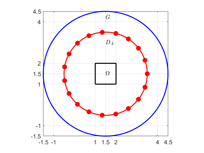
Figure 1: A schematic diagram of our measurement setup. The small black square indicates the domain $\Omega$ defined in (2.3). The large blue circle is the domain $G$ where the forward problem (2.10), (2.11) is solved to generate the data for the inverse problem. The red circle is the circle $C_{A}$ in (2.1) and small red discs on it indicate positions of the point source.

We choose $\rho=0.1$ in (2.5) for the function $f\left(\mathbf{x}-\mathbf{x}_{0}\right)$. For the conductivity coefficient $\sigma(\mathbf{x})$ to be reconstructed, we set

$$\sigma(\mathbf{x})=\left\{\begin{array}[]{cc}\sigma_{a}=const.>1,&\mbox{inside the tested inclusion,}\\ 1,&\mbox{outside the tested inclusion.}\end{array}\right.$$ (8.1)

To make sure $\sigma\left(\mathbf{x}\right)\in C^{1}\left(\overline{G}\right)$, we slightly smooth out $\sigma\left(\mathbf{x}\right)$ near the boundaries of our tested inclusions. Then we set:

$$\hskip-14.22636pt\mbox{correct inclusion/background contrast}=\frac{\sigma_{a}}{1},$$ (8.2)

$$\hskip-28.45274pt\mbox{computed inclusion/background contrast}=\frac{\max_{\mbox{inclusion}}\left(\sigma_{\mbox{comp}}(\mathbf{x})\right)}{1},$$ (8.3)

where $\sigma_{\mbox{comp}}(\mathbf{x})$ is the computed coefficient $\sigma(\mathbf{x}).$ In the numerical tests below, we take $\sigma_{a}=2,4$,$8$ which correspond to 2:1, 4:1 and 8:1 inclusion/background contrasts respectively. In the first series of numerical experiments we test the inclusions with the shapes of the letters ‘$A$’ and ‘$\Omega$’. In the second series we test the shapes of CT scans of an abdomen.

We choose the finite element method with $h=1/160$ to solve the forward problem in (2.10)-(2.11). For the source position $\mathbf{x}_{0}\in C_{A}$ in (3.11), we choose $\varphi=nh_{\varphi}$, $n=1,2,\cdots,199$, $h_{\varphi}=\pi/100$ . When the inclusion in (8.1) has the shape of the letter ‘$A$’ with $\sigma_{a}=2$, the results of the solution of the forward problem of $\mathbf{x}\in G$ and for four positions of the source

$$\mathbf{x}_{0}=(x_{0},y_{0})=(3.5,1.5),(1.5,3.5),(-0.5,1.5),(1.5,-0.5)$$

are displayed in Figure 2.

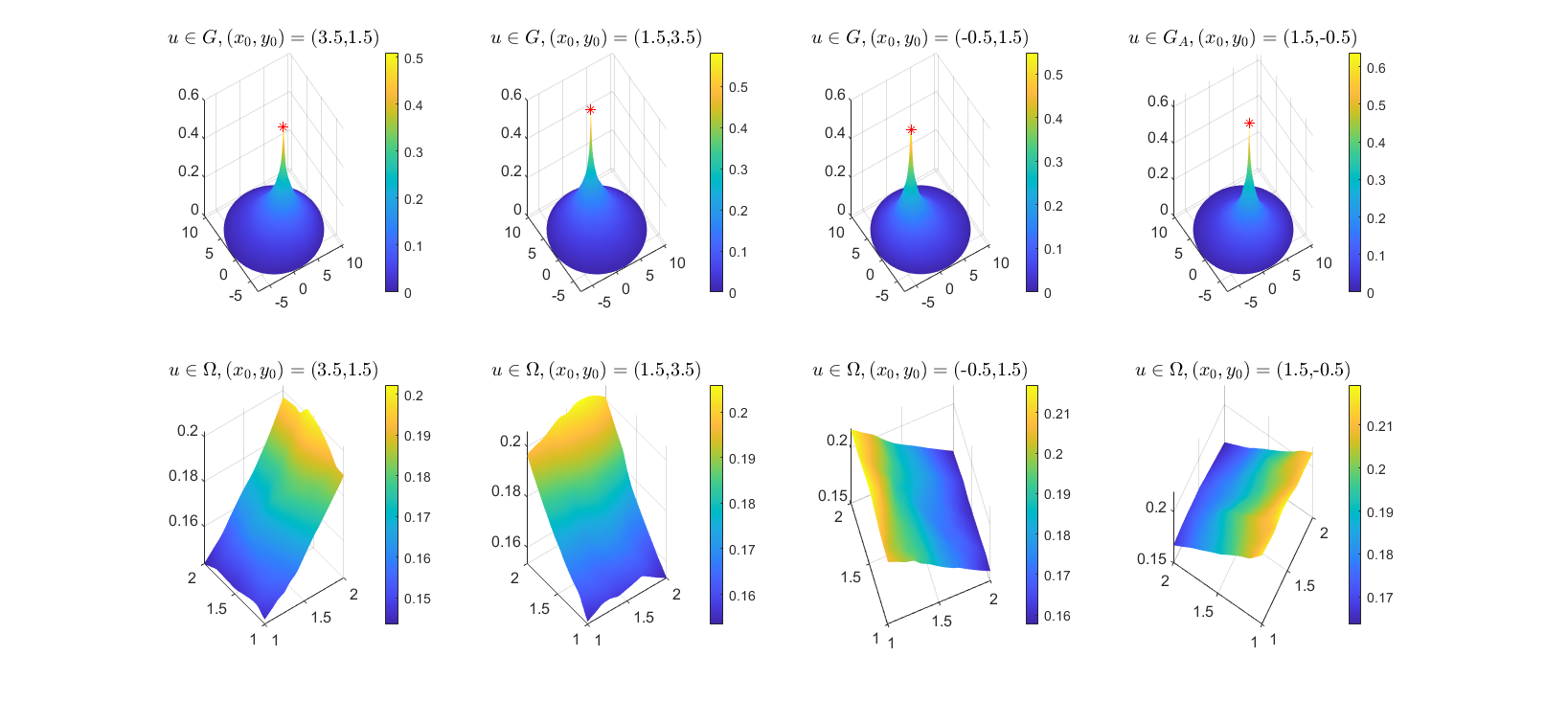
Figure 2: The results of the solution of the forward problem (2.10), (2.11) for the case when the inclusion has the shape of the letter ‘$A$’ with $\sigma_{a}=2$ inside of this letter, see (8.1). Top $\mathbf{x}\in G$, bottom $\mathbf{x}\in\Omega.$ The positions of the source are: $\mathbf{x}_{0}=(3.5,1.5)$ (1st column), $\mathbf{x}_{0}=(1.5,3.5)$ (2nd column), $\mathbf{x}_{0}=(-0.5,1.5)$ (3rt column), $\mathbf{x}_{0}=(1.5,-0.5)$ (4th column). The red star is the source position.

To solve Coefficient Inverse Problem (2.13), we have chosen the spatial mesh sizes in the computations of the Minimization Problem 1 in (4.5) and the Minimization Problem 2 in (4.10) as $1/40\times 1/40$. In both functionals $J_{\lambda,\alpha}\left(r,s\right)\left(\varphi\right)$ and $K\left(V\right)$ we write the differential operators in the forms of finite differences and minimize the resulting discretized functionals with respect to the values of corresponding functions at grid points. Since $H^{3}\left(\Omega\right)-$norms are inconvenient for the numerical implementation, we replace in (4.5) the regularization term $\alpha\left\|\left(r,s\right)\left(\mathbf{x},\varphi\right)\right\|_{H^{3}\left(\Omega\right)\times H^{3}\left(\Omega\right)}^{2}$ with $\alpha\left\|\left(r,s\right)\left(\mathbf{x},\varphi\right)\right\|_{H^{2}\left(\Omega\right)\times H^{2}\left(\Omega\right)}^{2}.$ Since we actually work with not too many grid points and since norms in finite dimensional spaces are equivalent, then this replacement did have a negative impact on our numerical results. An extension of the above theory on the discrete case is outside of the scope of this publication.

To guarantee that the solution of the problem of the minimization of the functional $J_{\lambda,\alpha}\left(r,s\right)\left(\varphi\right)$ in (4.5) satisfies the boundary conditions (3.21)-(3.24), we adopt the Matlab’s built-in optimization toolbox fmincon to minimize the discretized form of these corresponding functions. The same is true for the Minimization Problem 2.

The iterations of fmincon stop when the condition

$$|\nabla J_{\lambda,\alpha}\left(r,s\right)\left(\varphi\right)|<10^{-2},\quad|\nabla K(V)|<10^{-2}$$ (8.4)

are met. An explanation of the stopping criterion (8.4) is provided below.

We introduce the random noise in the observation data in (2.13) as follows:

$$\left.\begin{array}[]{c}g_{0}^{\xi_{0}}\left(\mathbf{x},\mathbf{x}_{0}\right)=g_{0}\left(\mathbf{x},\mathbf{x}_{0}\right)\left(1+\delta\xi_{0}\left(\mathbf{x}\right)\right),\quad\mathbf{x}\in\partial\Omega,\\ g_{1}^{\xi_{1}}\left(\mathbf{x},\mathbf{x}_{0}\right)=g_{1}\left(\mathbf{x},\mathbf{x}_{0}\right)\left(1+\delta\xi_{1}\left(\mathbf{x}\right)\right),\quad\mathbf{x}\in\Gamma,\end{array}\right.$$ (8.5)

where $\xi_{0}$ is the uniformly distributed random variable in the interval $[-1,1]$ depending on the point $\mathbf{x}\in\partial\Omega$. Also, $\xi_{1}$ is the uniformly distributed random variable in the interval $[-1,1]$ depending on the point $\mathbf{x}\in\Gamma$, and $\delta=0.03$ corresponds to the $3\%$ noise level. Since we deal with the first $\varphi-$derivatives of the noisy functions $g_{0}^{\xi_{0}}\left(\mathbf{x},\mathbf{x}_{0}\right)$ and $g_{1}^{\xi_{1}}\left(\mathbf{x},\mathbf{x}_{0}\right)$, we have to design a numerical method to differentiate the noisy data. First, we use the natural cubic splines to approximate the noisy input data (8.5). Next, we use the derivatives of those splines to approximate the derivatives of corresponding noisy observation data. We generate the corresponding cubic splines in $(0,2\pi)$ with the mesh grid size $h_{\varphi}=\pi/100$, and then we calculate their derivatives to approximate the first derivatives with respect to $\varphi$.

We choose the optimal pair of parameters $\left(\alpha,\varepsilon\right)$ by the trial and error procedure for the reference Test 1. For each considered pair $\left(\alpha,\varepsilon\right),$ we test different values of the parameter $\lambda$ to obtain its optimal value $\lambda_{\mbox{opt}}\left(\alpha,\varepsilon\right)$ for this pair. Once the so chosen triple $\left(\alpha,\varepsilon,\lambda\right)$ of parameters is selected, we consider it as the optimal choice of parameters. An important point to make here is that exactly the same triple of optimal parameters is used for all follow up tests when imaging letters below. However, when using the CT scan of the abdomen below, we deal with a different medium. This means that we repeat the procedure of our choice of parameters again for this case.

Remarks 8.1:

1. As the test media, we intentionally choose letter-like shapes of inclusions in the first series of numerical experiments and the CT scans of the abdomen in the second series. This is done to demonstrate that our technique works well for complicated media.

2. The above procedure of the choice of an optimal triple $\left(\alpha,\varepsilon,\lambda\right)$ of parameters is similar to the conventional calibration procedure, which is often used in many real World applications. Furthermore, quite similar procedures were used in all above cited works [18, 19, 20, 22, 23, 24] on the numerical studies of the convexification method for CIPs.

3. Even though theorems of our convergence analysis are valid only for sufficiently large values of the parameter $\lambda,$ we have discovered in all our works on the convexification listed in item 2 that actually optimal values of $\lambda$ belong to the interval $\lambda\in\left[1,5\right].$ In fact, this is similar with many asymptotic theories. Indeed, it is typically established in such a theory that if a certain parameter $X$ is sufficiently large, then a certain formula $Y$ provides a good approximation for a process. However, it is also typical that in a computational practice only numerical experiments can tell one which exactly values of $X$ are appropriate ones.

Test 1. We test the case when the inclusion in (8.1) has the shape of the letter ‘$A$’ with $\sigma_{a}=2$ inside of it. We use this test as a reference one to figure out the optimal triple $\left(\alpha,\varepsilon,\lambda\right)$ of parameters. We have found that this triple is

$$\alpha=0.01,\varepsilon=0.0002,\lambda=3.$$ (8.6)

This is our optimal choice of parameters for the case when inclusions have letter-like shapes.

Figure 3 shows how do we choose the optimal value of $\lambda$ once the optimal pair $\left(\alpha,\varepsilon\right)$ is selected as in (8.6). We observe that the images have a low quality for $\lambda=0,1,2$. Then the quality is improved with $\lambda=3,4,5$, and the reconstruction quality deteriorates at $\lambda=10$. On the other hand, the image is accurate at $\lambda=3$, including the accurate reconstruction of the inclusion/background contrast (8.2).

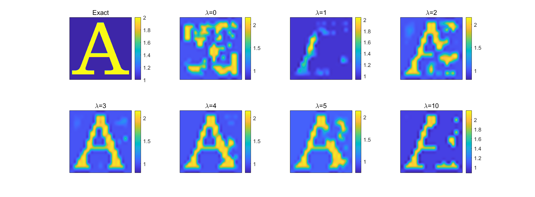
Figure 3: Test 1. The reconstructed coefficient $\sigma(\mathbf{x})$, where the function $\sigma(\mathbf{x})$ is given in (8.1) with $\sigma_{a}=2$ inside of the letter ‘A’. We test different values of $\lambda$.

We display now in Figure 4 the convergence behavior of $|\nabla J_{\lambda,\alpha}(r,s)(\varphi)|$ with respect to the iterations of fmincon for $\varphi=\pi$ and for the optimal triple $\left(\alpha,\varepsilon,\lambda\right)$ of parameters as in (8.6). This figure explains the stopping criterion (8.4).

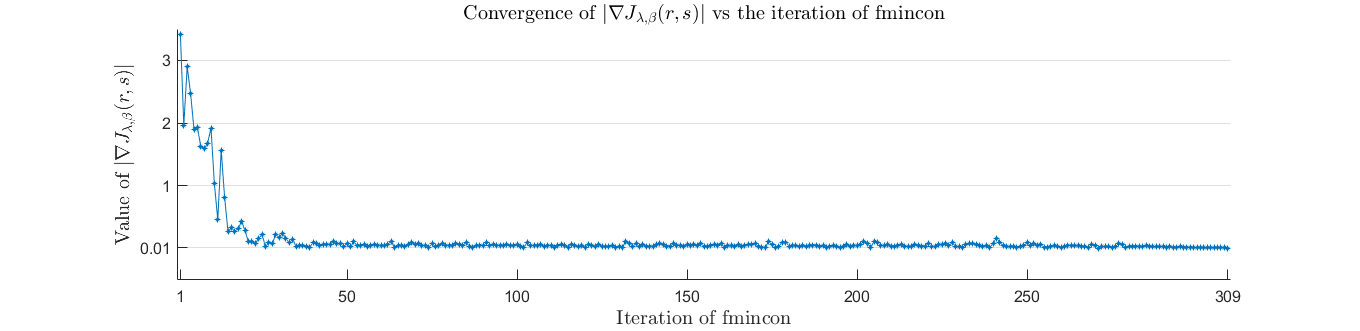
Figure 4: Test 1. The convergence behavior of $\left|\nabla J_{\lambda,\alpha}\left(r,s\right)\left(\varphi\right)\right|$ with the iterations of fmincon for $\varphi=\pi$ and the optimal triple of parameters $\left(\alpha,\varepsilon,\lambda\right)$ as in (8.6). The function $\sigma\left(\mathbf{x}\right)$ is given in (8.1) with $\sigma_{a}=2$ inside of the letter ‘$A$’. The $y-$axis corresponds to the value of $\left|\nabla J_{\lambda,\alpha}\left(r,s\right)\left(\varphi\right)\right|$.

Test 2. We test the case when the inclusion in (8.1) has the shape of the letter ‘$A$’ for different values of the parameter $\sigma_{a}=4,8$ inside of the letter ‘$A$’. Hence, by (8.2) the inclusion/background contrasts now are respectively $4:1$ and $8:1$. Computational results are displayed on Figure 5. One can observe that shapes of inclusions are imaged accurately. In addition, the computed inclusion/background contrasts (8.2) are accurate.

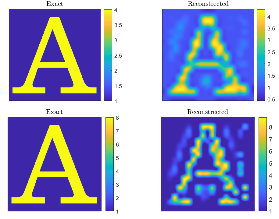
Figure 5: Test 2. Exact (left) and reconstructed (right) coefficient $\sigma(\mathbf{x})$ with $\sigma_{a}=4$ (first row) and $\sigma_{a}=8$ (second row) inside of the letter ‘A’ as in (8.1). The inclusion/background contrasts in (8.2) are respectively $4:1$ and $8:1$. The reconstructions of both shapes of inclusions and the inclusion/background contrasts (8.2) are accurate, although the image in the second row is more blurred.

Test 3. We test the case when the coefficient $\sigma(\mathbf{x})$ in (8.1) has the shape of the letter ‘$\Omega$’ with $\sigma_{a}=2$ inside of it. Results are presented on Figure 6. We again observe an accurate reconstruction.

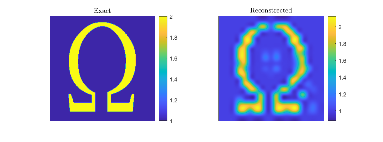
Figure 6: Test 3. Exact (left) and reconstructed (right) coefficient $\sigma(\mathbf{x})$, where the function $\sigma(\mathbf{x})$ is given in (8.1) with $\sigma_{a}=2$ inside of the letter ‘$\Omega$’. The reconstructions of both the shape of the inclusions and the inclusion/background contrast (8.2) are accurate.

Test 4. We consider the case when the random noisy is present in the data in (8.5) with $\delta=0.03$, i.e. with the 3% noise level. We test the reconstruction for the cases when the inclusion in (8.1) has the shape of either the letter ‘$A$’ or the letter ‘$\Omega$’ with $\sigma_{a}=2$ inside of them. The results are displayed on Figure 7. One can observe accurate reconstructions in all four cases. In particular, the inclusion/background contrasts in (8.2) are reconstructed accurately.

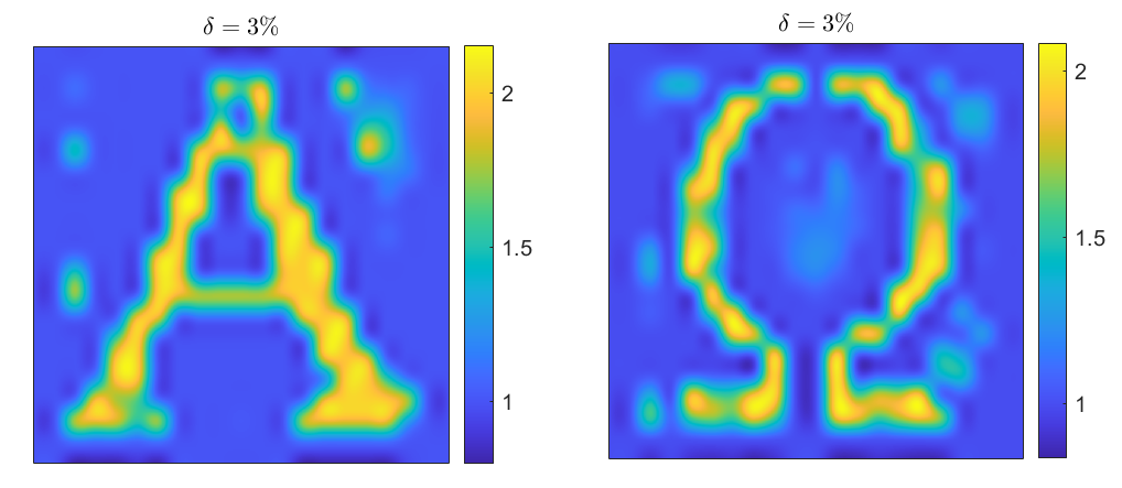
Figure 7: Test 4. Reconstructed coefficient $\sigma(\mathbf{x})$ with the shape of letters ‘A’ (left) or the letter ‘$\Omega$’ (right) with $\sigma_{a}=2$ from noisy data (8.5) with $\delta=0.03$, i.e. with 3% noise level. The reconstructions of both shapes of inclusions and inclusion/background contrasts in (8.2) are accurate.

Test 5. In this test, we verify the numerical method for the case, which is both more complex and more practical one. More precisely, we consider now the case when the coefficient $\sigma(\mathbf{x})$ in (8.1) has the shape of a CT scan of an abdomen. We obtain the CT image and the corresponding segmented image from [27]. The conductivity distributions in [27] range from 2 to 10. However, using a linear transformation, we obtain the coefficient $\sigma(\mathbf{x})$ in (8.1) with $\sigma_{a}=2$.

Since this is a completely new set of images, then we need to calibrate our method again, see item 2 of Remarks 8.1. Hence, we need to select a new optimal triple $\left(\alpha,\varepsilon,\lambda\right)$ of parameters. We use the same trial and error procedure as the one described above. The resulting optimal parameters are:

$$\alpha=0.02,\varepsilon=0.0005,\lambda=2.5.$$ (8.7)

The solution of our CIP for this case is presented on Figure 8, where the left image is exactly the segmented image of [27]. One can observe an accurate reconstruction.

Next, we test the optimal triple (8.7) of parameters for the segmented CT scan of [27], in which, however, we take $\sigma_{a}=3,$ unlike $\sigma_{a}=2$ of the previous case. The reconstructed image is displayed on Figure 9. The reconstruction is accurate again.

Finally, we use the set of parameters (8.7) to solve our CIP for the case of a more complicated segmented abdominal image, which we again take from [27]. The CT scan is displayed on the left Figure 10. The corresponding segmented image is displayed on the middle Figure 10. One can observe a range of colors here from dark blue to yellow, which indicates that this case is more complicated than the ones of two previous images. Our reconstructed image is presented on the right Figure 10. One can observe that the reconstruction is rather accurate even for this complicated case with many colors.

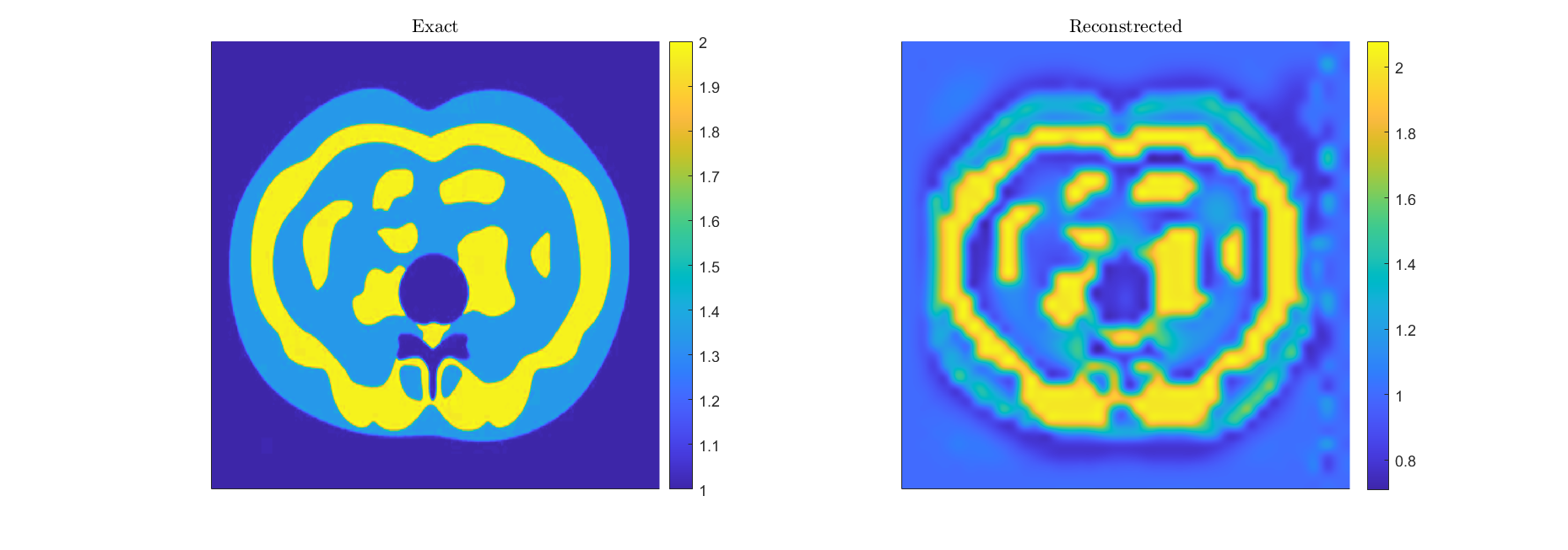
Figure 8: Test 5. Abdominal exact segmented image (left) and reconstructed (right) coefficient $\sigma(\mathbf{x})$, where the function $\sigma(\mathbf{x})$ is given in (8.1) with $\sigma_{a}=2$ with the shape of an abdomen. The reconstructions of both the shape of the inclusions and the inclusion/background contrast (8.2) are accurate.

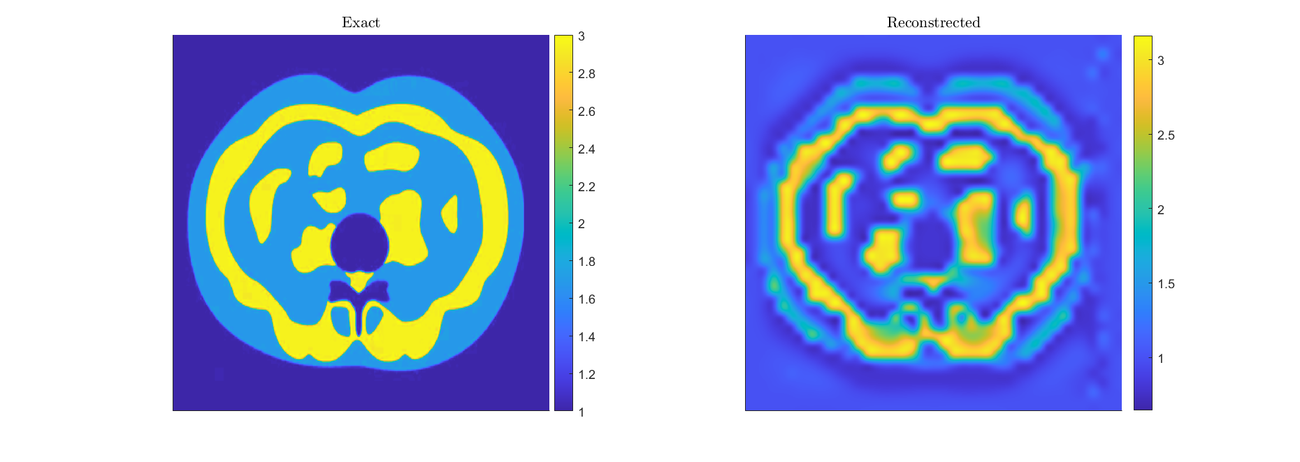
Figure 9: Test 5. Abdominal exact segmented image (left) and reconstructed (right) coefficient $\sigma(\mathbf{x})$, where the function $\sigma(\mathbf{x})$ is given in (8.1) with $\sigma_{a}=3$ with the shape of an abdomen. The reconstructions of both the shape of the inclusions and the inclusion/background contrast (8.2) are approximately good.

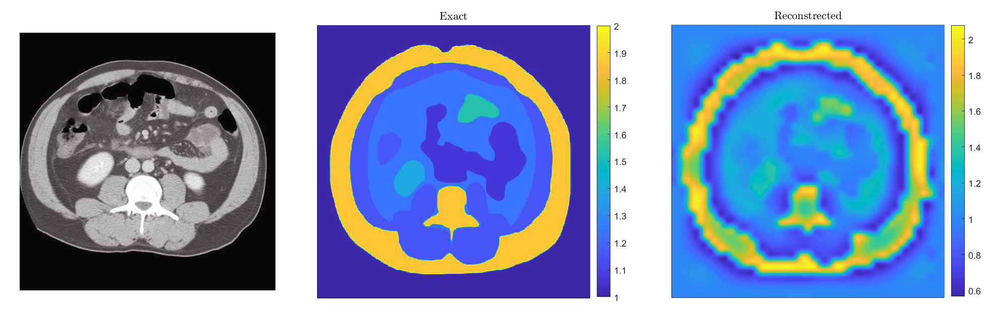
Figure 10: Test 5. Abdominal CI image (left), corresponding segmented image (middle) and reconstructed (right) coefficient $\sigma(\mathbf{x})$, where the function $\sigma(\mathbf{x})$ is given in (8.1) with $\sigma_{a}=2$ with the shape of a CT scan of an abdomen. The reconstruction is rather accurate even for this complicated case with many colors.

References

References

- [1] L. Beilina. Domain decomposition finite element/finite difference method for the conductivity reconstruction in a hyperbolic equation. Communications in Nonlinear Science and Numerical Simulation, 37:222–237, 2016.
- [2] L. Beilina, M. G. Aram, and E. M. Karchevskii. An adaptive finite element method for solving 3D electromagnetic volume integral equation with applications in microwave thermometry. J. Comput. Phys., 459:111122, 2022.
- [3] L. Beilina and E. Lindström. An adaptive finite element/finite difference domain decomposition method for applications in microwave imaging. Electronics, 11:1359, 2022.
- [4] G. Chavent. Nonlinear Least Squares for Inverse Problems: Theoretical Foundations and Step-by-Step Guide for Applications. Springer Science & Business Media, Berlin, 2010.
- [5] M. Gehre, B. Jin, and X. Lu. An analysis of finite element approximation in electrical impedance tomography. Inverse Problems, 30(4):045013, 3 2014.
- [6] G. Gilbarg and N. S. Trudinger. Elliptic Partial Differential Equations of Second Order. Springer-Verlag, New York, second edition, 1983.
- [7] G. Giorgi, M. Brignone, R. Aramini, and M. Piana. Application of the inhomogeneous Lippmann–Schwinger equation to inverse scattering problems. SIAM J. Appl. Math., 73:212–231, 2013.
- [8] A. V. Goncharsky and S. Y. Romanov. Iterative methods for solving coefficient inverse problems of wave tomography in models with attenuation. Inverse Probl., 33:025003, 2017.
- [9] A. V. Goncharsky, S. Y. Romanov, and S. Y. Seryozhnikov. On mathematical problems of two-coefficient inverse problems of ultrasonic tomography. Inverse Probl., 40:045026, 2024.
- [10] M. J. Grote and U. Nahum. Adaptive eigenspace for multi-parameter inverse scattering problems. Computers & Mathematics with Applications, 77:3264–3280, 2019.
- [11] S. J. Hamilton, J. M. Reyes, S. Siltanen, and X. Zhang. A Hybrid Segmentation and D-Bar Method for Electrical Impedance Tomography. SIAM Journal on Imaging Sciences, 9(2):770–793, 2016.
- [12] B. Harrah. The Calderon problem with finitely many unknowns is equivalent to convex semidifinite optimization. SIAM J. Mathematical Analysis, 55:5666–5684, 2023.
- [13] B. Harrah and H. Meftahi. A monotonicity-based globalization of the level-set method for inclusion detection. arXiv:2501.15887, 2025.
- [14] B. Harrah and A. Brojatsch. On the required number of electrodes for uniqueness and convex reformulation in an inverse coefficient problem. arXiv:2411.00482, 2025.
- [15] D. Holder. Electrical Impedance Tomography: Methods, History and Applications. Bristol: Institute of Physics, 2005.
- [16] M. V. Klibanov. Convexification of restricted Dirichlet to Neumann map. J. Inverse Ill-Posed Probl., 25:669–685, 2017.
- [17] M. V. Klibanov and O. V. Ioussoupova. Uniform strict convexity of a cost functional for three-dimensional inverse scattering problem. SIAM J. Math. Anal, 26:147–179, 1995.
- [18] M. V. Klibanov, V. A. Khoa, A. V. Smirnov, L. H. Nguyen, G. W. Bidney, L. Nguyen, A. Sullivan, and V. N. Astratov. Convexification inversion method for nonlinear SAR imaging with experimentally collected data. J. Appl. Ind. Math., 15:413–436, 2021.
- [19] M. V. Klibanov, J. Li, and W. Zhang. Electrical impedance tomography with restricted Dirichlet-to-Neumann map data. Inverse Probl., 35:035005, 2019.
- [20] M. V. Klibanov and J. Li. Inverse Problems and Carleman Estimates: Global Uniqueness, Global Convergence and Experimental Data. De Gruyter, Berlin, 2021.
- [21] M. V. Klibanov, L. H. Nguyen, and H. V. Tran. Numerical viscosity solutions to Hamilton-Jacobi equations via a Carleman estimate and the convexification method. Journal of Computational Physics, 451:110828, 2021.
- [22] M. V. Klibanov, J. Li, L.H. Nguyen, and Z. Yang. Convexification numerical method for a coefficient inverse problem for the radiative transport equation. SIAM J. Imag. Sci., 16:35–63, 1 2023.
- [23] M. V. Klibanov, J. Li, and Z. Yang. Convexification for the viscosity solution for a coefficient inverse problem for the radiative transport equation. Inverse Problems, 39:125002, 2023.
- [24] M. V. Klibanov, J. Li, and Z. Yang. Convexification numerical method for a coefficient inverse problem for the system of nonlinear parabolic equations governing mean field games. Inverse Problems and Imaging, 19:219–252, 2025.
- [25] O. A. Ladyzhenskaya and N. N. Uralceva. Linear and Quasilinear Elliptic Equations. Academic Press, New York, 1969.
- [26] H.P.N. Le, T. T. Le, and L. H. Nguyen. The Carleman convexification method for Hamilton-Jacobi equations. Computers & Mathematics with Applications, 159:173–185, 2024.
- [27] K. Lee, M. Yoo, A. Jargal, and H. Kwon. Electrical Impedance Tomography-Based Abdominal Subcutaneous Fat Estimation Method Using Deep Learning. Computational and Mathematical Methods in Medicine, 2020:1–14, 2020.
- [28] E. Lindström and L. Beilina. Energy norm error estimates and convergence analysis for a stabilized Maxwell’s equations in conductive media. Electronics, 69:415–436, 2024.
- [29] J. L. Mueller and S. Siltanen. The D-bar method for electrical impedance tomography-demystified. Inverse Problems, 36:093001, 2020.
- [30] G. Rizutti and A. Gisolf. An iterative method for 2D inverse scattering problems by alternating reconstruction of medium properties and wavelets: theory and application to the inversion of elastic waveforms. Inverse Problems, 33:035003, 2017.
- [31] A. N. Tikhonov and V. Y. Arsenin. Solutions of Ill-Posed Problems. Winston, New York, 1977.
- [32] A. N. Tikhonov, A. V. Goncharsky, V. V. Stepanov, and A. G. Yagola. Numerical methods for the solution of Ill-posed problems. Kluwer, London, 1995.