Co-Optimizing Distributed Energy Resources under Demand Charges and Bi-Directional Power Flow
Abstract
We address the co-optimization of behind-the-meter (BTM) distributed energy resources (DER), including flexible demands, renewable distributed generation (DG), and battery energy storage systems (BESS) under net energy metering (NEM) frameworks with demand charges. We formulate the problem as a stochastic dynamic program that accounts for renewable generation uncertainty and operational surplus maximization. Our theoretical analysis reveals that the optimal policy follows a threshold structure. Finally, we show that even a simple algorithm leveraging this threshold structure performs well in simulation, emphasizing its importance in developing near-optimal algorithms. These findings provide crucial insights for implementing prosumer energy management systems under complex tariff structures.
Index Terms:
Battery storage systems, distributed energy resources, dynamic programming, energy management systems, flexible demands, Markov decision process, net energy metering.I Background and Literature
A clean, resilient, and sustainable energy system requires optimal coordination of BTM DER, such as DG, flexible demands, and BESS [1]. Economic and technical aspects are the main drivers for BTM DER operation and coordination. Under NEM, prosumers can bi-directionally transact energy and money with the distribution utility (DU), who levy a buy (retail) rate or a sell (export) rate based on net-consumption – gross demand minus gross generation [2].
With the increasing penetration of new and large electric loads such as electric vehicles, electric ovens, and heat pumps, DUs are increasingly supplementing volumetric charges111Charges based on the total net consumption of energy. with demand charges. These are defined as $/kW fees imposed on the peak demand recorded during a billing cycle and are introduced to encourage smoother load profiles and reduce the operational costs of grid maintenance [3].222Demand charges differ from critical peak pricing, a form of time-varying pricing aimed at incentivizing load shedding during critical periods [4]. With the growing adoption of demand charges, several studies have highlighted the role of BTM DER in helping customers mitigate them [5].
This work focuses on the co-optimization of BTM DER, including flexible demand, renewable DG, and BESS, under NEM frameworks with differentiated buy and sell rates and demand charges (Fig. 1). A comparative overview of related studies in terms of demand flexibility, storage integration, NEM capabilities, and demand charges is provided in Table I. To the best of our knowledge, this work is the first to co-optimize flexible demand and storage operations under the combined presence of NEM and demand charges.
Previous research has addressed aspects of this problem. In [6, 7], dynamic programming was employed to minimize prosumer costs by optimally scheduling BESS operation under inelastic demand. Also, the co-optimization of demand flexibility and BESS was considered in [8, 9], though without incorporating the ability of prosumers to buy and sell energy under NEM. Studies such as [10, 11, 12, 13] incorporate the NEM buy-and-sell feature, optimizing storage scheduling in [10], and jointly optimizing storage and flexible demand in [11, 12, 13]. However, these works ignore demand charges, which significantly complicates the scheduling problem.
In contrast, while [3, 14] integrate demand charges in their optimization models, the assumed free disposal of surplus renewables eliminates NEM’s bidirectional energy transactions, which is a critical limitation given the growing real-world prevalence of such interactions.
Contributions. This paper advances research on optimal scheduling of BTM DERs with three key contributions:
-
1.
We develop a stochastic dynamic programming framework that jointly optimizes demand scheduling and BESS under NEM and demand charge constraints, maximizing prosumer operational surplus.
-
2.
We prove that the optimal policy maintains a threshold structure consistent with prior work while demonstrating how integrating multiple factors—demand flexibility, storage, and demand charges—leads to exponential computational complexity in the number of flexible demands.
-
3.
Through extensive simulations against baseline approaches, we demonstrate how leveraging the threshold structure properties enables the development of computationally efficient near-optimal algorithms.
II Problem Formulation
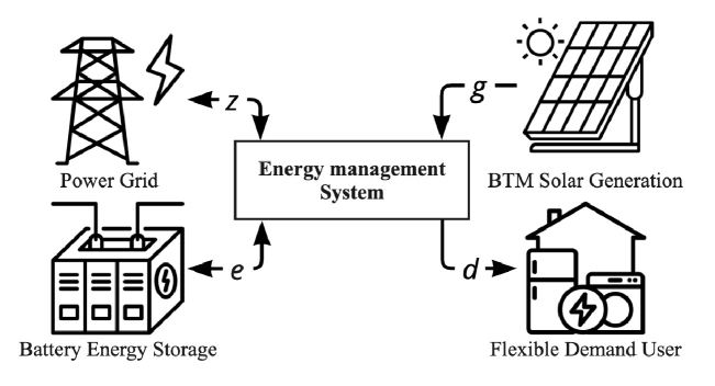
We study an energy management system (EMS) for prosumers that co-optimizes flexible demand, storage operation, and renewable distributed generation under a NEM tariff with distinct buy/sell rates and peak demand charges. The optimization objective maximizes the net benefit defined as consumption utility minus electricity costs, where demand charges are levied on the maximum consumption drawn from either load, battery charging, or both. As shown in Fig. 1, this dynamic programming formulation explicitly accounts for the temporal coupling of storage operations and an NEM tariff with bidirectional energy pricing and peak demand charges.
II-A Prosumer Resources
We consider the operation over a discrete and finite time horizon . As shown in Fig.1, the prosumer has BTM renewable DG, denoted by . The renewable DG is modeled as an exogenous (positive) Markov random process.
The flexible demands are denoted by the vector
| (1) |
where is the total number of prosumer devices. Here is the consumption bundle’s upper limit.
The prosumer also owns a BTM battery energy storage, which has output , where and are discharging and charging limits. The output is decomposed into charging and discharging . With charge/discharge efficiencies , the state of charge (SoC) evolves as:
| (2) |
where denotes battery capacity.
The net energy consumption of the prosumer at time is
| (3) |
Therefore, the prosumer imports power from the grid if and exports power to the grid if .
II-B System Dynamics
The system state at time , , is described as
| (4) |
where is the prosumer’s peak demand before time . We allow the system to be controlled by battery charging/discharging and consumption adjustments, i.e., the control action is
| (5) |
II-C NEM X Tariff with Demand Charges
Under NEM, when the prosumer’s gross loads (from consumption and storage charging) are higher than its generation (from renewable DG), the prosumer pays at the retail rate. Otherwise, the prosumer gets compensated at the export rate.
Let be the retail, export, and peak demand prices, respectively. We equivalently break down the peak demand charge at the end of time to each time step since . Thus, we can write the payment (cost) under NEM X in [2] for each time as
| (7) |
where () signifies a payment by the prosumer (DU) to the DU (prosumer).
II-D Flexible Demands and Storage Co-Optimization
At each time step , the prosumer’s utility of consuming is given by an additive utility function
| (8) |
that is assumed to be concave and continuously differentiable.
We define the reward function of the dynamic program as the difference between satisfaction from consumption (8) and payment (7). Therefore, the reward function is
| (9) |
To encourage the preservation of energy in the battery, we define a linear reward to the remaining energy at step , i.e.
| (10) |
for a . The salvage value rate influences optimal DER scheduling. Here, we assume , deferring analysis of ’s impact to future work.
The policy is a sequence of mapping from state space to action space such that . Given initial state , the storage-consumption co-optimization is then defined as:
| (11a) | ||||
| Subject to | ||||
| (11b) | ||||
| (11c) | ||||
| (11d) | ||||
| (11e) | ||||
| (11f) | ||||
| (11g) | ||||
| (11h) | ||||
| (11i) | ||||
Note: (11e) and (11h) introduce strong temporal dependencies.
The value function is defined as the total reward received under the policy , i.e., . The optimal value function is defined as .
III Dynamic Program Analytical Results
In this section, we show that the optimal policy for the co-optimization problem in Sec. II is a threshold policy.
The following lemma establishes a conclusion regarding the concavity of the optimal value function.
Lemma 1.
The optimal value function is concave in for every time step .
Proof.
We follow the proof technique for lemma 1 in [3].
Consider two different states and with their corresponding optimal trajectories and . Let be their average initial state, and define the average policy with corresponding trajectory .
It turns out that the optimal value function is also non-decreasing in the system state.
Lemma 2.
The optimal value function is non-decreasing in , , and for every time step .
Proof.
(1) : Consider two SoCs , such that , . Let be the optimal action sequence for SoC . If there exists , , action sequence is feasible for SoC . Hence . Otherwise, , , so action sequence is feasible for SoC , .
(2) : Consider two generations , . Let be the optimal action sequence for generation . Apply the action sequence to generation , , .
(3) : From (7), is non-increasing in , hence is non-decreasing in . ∎
Lastly, we derive a property that links the optimal Q-function, defined as , to the system’s control action .
Lemma 3.
The optimal Q-function is concave in .
Proof.
For , let be the trajectory of and be the trajectory of . By (12) - (14), applying actions to gives:
| (16) | ||||
Therefore, is concave in . ∎
Lem. 1 to Lem. 3 lead to Thm. 1 about the structure of the optimal co-optimization policy under demand charges.
Theorem 1.
For each step , the optimal policy is a threshold policy.
Proof.
The feasible region for action , is a compact set. From Lem. 1 to Lem. 3, the optimal value function and Q-function is concave in action , so the optimal action
| (17) |
must exist in the interior of the feasible set or at the boundary of the feasible set . The optimal action can be obtained by solving concave optimizations with and without boundary constraints, which results in a threshold policy. ∎
Although Thm. 1 reveals a structured policy, direct dynamic programming implementation remains impractical. First, optimization necessitates gradients of and , which are computationally prohibitive for complex utilities. Also, continuous-space Q-function tracking requires costly discretization, as validated in simpler settings [3]. We thus employ reinforcement learning (RL) to approximate the optimal policy efficiently.
IV Case Study
We investigate the effectiveness and efficiency of RL in solving this co-optimization problem. We compare Proximal Policy Optimization (PPO) [15] against Tesla’s backup mode [16], a threshold algorithm, and the optimal nonlinear program in simulation. Experiments were run on a server with 1 AMD Ryzen Threadripper 3990X 64-Core Processor and 4 Nvidia RTX A4000 GPUs.
IV-A Problem Setup
We adopt the concave utility function from [17]: , where , dynamically reflect the electricity costs and demand elasticity. The elasticity is set to -0.1 for an inelastic user [18]. Baseline battery parameters are set as kWh, kW with efficiencies . Electricity price is assumed static of for buying, for selling, and for daily peak demand charge.
IV-B Control Strategies
Baseline
The Tesla’s backup mode maintains a full battery by charging and only discharges during grid outages. It shows what would happen without a battery system [3].
Reinforcement Learning using PPO
The PPO algorithm uses an actor network and a critic network with the same Multilayer Perceptron (MLP) structure. For this case study, we used the default MLP policy from stable baseline [19].
Threshold Algorithm
Based on the optimal structure, we developed a simple threshold algorithm as follows:
| (18) |
and in both cases.
Nonlinear Program
Formulate the battery-demand co-optimization as a deterministic nonlinear program solved with Gurobi. It provides the optimal value for comparison.
IV-C Dataset
IV-D Results
| Scenario | Method | ||||||
| Generation | Demand | Battery Capacity | Charge/Discharge Limits | Backup | Threshold | PPO | Optimal |
| 25th Percentile | 75th Percentile | 5kWh | 1kW | 8.7 (0%) | 10.3 (18.4%) | 15.7 (80.5%) | 20.3 (133.3%) |
| 50th Percentile | 50th Percentile | 5kWh | 1kW | 10.4 (0%) | 11.9 (14.4%) | 17.2 (65.4%) | 21.9 (110.6%) |
| 75th Percentile | 25th Percentile | 5kWh | 1kW | 10.7 (0%) | 12.2 (14.0%) | 17.0 (58.9%) | 22.0 (105.6%) |
| 50th Percentile | 50th Percentile | 3kWh | 1kW | 10.4 (0%) | 11.2 (7.7%) | 14.8 (42.3%) | 19.8 (90.4%) |
| 50th Percentile | 50th Percentile | 7kWh | 1kW | 10.4 (0%) | 21.5 (106.7%) | 17.9 (72.1%) | 22.5(116.3%) |
| 50th Percentile | 50th Percentile | 5kWh | 0.5kW | 10.4 (0%) | 16.0 (53.8%) | 16.2 (55.8%) | 20.2 (94.2%) |
| 50th Percentile | 50th Percentile | 5kWh | 2kW | 10.4 (0%) | 11.9 (14.3%) | 18.5 (77.9%) | 21.9 (110.6%) |
We evaluate seven scenarios by varying:
-
•
Generation/Demand: 25th–75th percentile solar generation paired with 75th–25th percentile demand to simulate energy-abundant/scarce conditions;
-
•
Battery Capacity: 3kWh - 7kWh capacity to simulate small/medium/large battery size.
-
•
Battery Charge/Discharge Limit: 0.5 kW - 2kW to simulate low charging/discharging rates to high rates.
Tab. II shows the performance comparisons across all scenarios. The results are evaluated using reward metrics, with percentage gains calculated relative to the Backup baseline. Under varying generation-demand scenarios with fixed battery parameters (5kWh, 1kW), PPO dominates the threshold method with 58.9-80.5% versus 14.0-18.4% gains, demonstrating adaptability to varying generation-demand conditions. The threshold algorithm is sensitive to the capacity, which is improved significantly (106.7% gain) due to reduced demand-side dependency when the capacity is large, where the optimal and threshold policies are similar. By contrast, PPO maintains the robustness. Higher limits also amplify potential gains. While PPO follows the trend, the threshold shows over-aggressive control, degrading performance significantly.
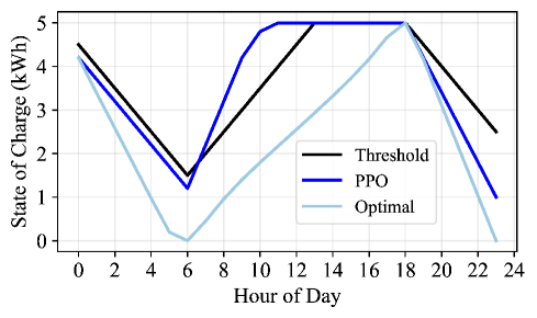
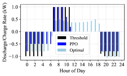
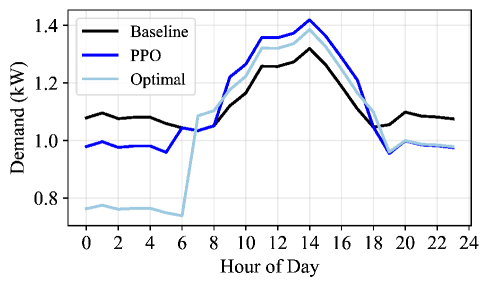
Fig. 3 shows the state and actions sequence of medium generation/demand and (5kWh, 1kW) battery configuration. Both threshold and RL policies align closely with optimal strategies in the scenario while being more aggressive in battery actions when lacking generation predictions. Key behavioral patterns include battery charging and demand elevation in the daytime to exploit solar surplus, and battery discharging and demand reduction in the evening to mitigate grid reliance.
V Conclusion
In conclusion, we presented a comprehensive investigation into the co-optimization of DERs in a realistic setting controlling both demands and energy storage under a bi-directional net metering pricing structure, including demand charge. We proposed a stochastic dynamic program to model the problem and proved the optimality of the threshold structure. Through simulations with real-world data, we demonstrated that the RL algorithm can achieve significant surplus gains compared to baseline approaches, highlighting the effectiveness of using RL to approximate optimal control for prosumer EMS.
References
- [1] M. F. Akorede, H. Hizam, and E. Pouresmaeil, “Distributed energy resources and benefits to the environment,” Renewable and Sustainable Energy Reviews, vol. 14, no. 2, pp. 724–734, Feb. 2010. [Online]. Available: https://linkinghub.elsevier.com/retrieve/pii/S1364032109002561
- [2] A. S. Alahmed and L. Tong, “On net energy metering X: Optimal prosumer decisions, social welfare, and cross-subsidies,” IEEE Trans. Smart Grid, vol. 14, no. 02, 2023.
- [3] J. Jin and Y. Xu, “Optimal Storage Operation Under Demand Charge,” IEEE Transactions on Power Systems, vol. 32, no. 1, pp. 795–808, Jan. 2017. [Online]. Available: http://ieeexplore.ieee.org/document/7452430/
- [4] J. L. Neufeld, “Price discrimination and the adoption of the electricity demand charge,” The Journal of Economic History, vol. 47, no. 3, pp. 693–709, 1987. [Online]. Available: http://www.jstor.org/stable/2121336
- [5] J. McLaren, P. Gagnon, and S. Mullendore, “Identifying potential markets for behind-the-meter battery energy storage: A survey of U.S. demand charges,” National Renewable Energy Laboratory, Tech. Rep., 2017. [Online]. Available: http://tiny.cc/NREL
- [6] P. Harsha and M. Dahleh, “Optimal management and sizing of energy storage under dynamic pricing for the efficient integration of renewable energy,” IEEE Transactions on Power Systems, vol. 30, no. 3, pp. 1164–1181, 2015.
- [7] N. Zhang, B. D. Leibowicz, and G. A. Hanasusanto, “Optimal residential battery storage operations using robust data-driven dynamic programming,” IEEE Transactions on Smart Grid, vol. 11, no. 2, pp. 1771–1780, 2020.
- [8] C. Chen, J. Wang, Y. Heo, and S. Kishore, “MPC-based appliance scheduling for residential building energy management controller,” IEEE Transactions on Smart Grid, vol. 4, no. 3, pp. 1401–1410, 2013.
- [9] R. Khezri, A. Mahmoudi, and M. H. Haque, “A demand side management approach for optimal sizing of standalone renewable-battery systems,” IEEE Transactions on Sustainable Energy, vol. 12, no. 4, pp. 2184–2194, 2021.
- [10] T. Li and M. Dong, “Residential energy storage management with bidirectional energy control,” IEEE Transactions on Smart Grid, vol. 10, no. 4, pp. 3596–3611, 2019.
- [11] Y. Xu and L. Tong, “Optimal Operation and Economic Value of Energy Storage at Consumer Locations,” IEEE Transactions on Automatic Control, vol. 62, no. 2, pp. 792–807, Feb. 2017. [Online]. Available: http://ieeexplore.ieee.org/document/7478023/
- [12] A. S. Alahmed, L. Tong, and Q. Zhao, “Co-Optimizing Distributed Energy Resources in Linear Complexity Under Net Energy Metering,” IEEE Transactions on Sustainable Energy, vol. 15, no. 4, pp. 2336–2348, Oct. 2024. [Online]. Available: https://ieeexplore.ieee.org/document/10568387/
- [13] B. Jeddi, Y. Mishra, and G. Ledwich, “Differential dynamic programming based home energy management scheduler,” IEEE Transactions on Sustainable Energy, vol. 11, no. 3, pp. 1427–1437, 2020.
- [14] F. Luo, W. Kong, G. Ranzi, and Z. Y. Dong, “Optimal home energy management system with demand charge tariff and appliance operational dependencies,” IEEE Transactions on Smart Grid, vol. 11, no. 1, pp. 4–14, 2020.
- [15] J. Schulman, F. Wolski, P. Dhariwal, A. Radford, and O. Klimov, “Proximal policy optimization algorithms,” arXiv preprint arXiv:1707.06347, 2017.
- [16] Tesla. (2024) Powerwall modes of operation with solar. Tesla, Inc. [Online]. Available: https://www.tesla.com/en_au/support/energy/powerwall/mobile-app/modes-of-operationwithsolar
- [17] A. S. Alahmed and L. Tong, “Integrating Distributed Energy Resources: Optimal Prosumer Decisions and Impacts of Net Metering Tariffs,” May 2022, arXiv:2204.06115. [Online]. Available: http://arxiv.org/abs/2204.06115
- [18] A. Asadinejad, A. Rahimpour, K. Tomsovic, H. Qi, and C.-f. Chen, “Evaluation of residential customer elasticity for incentive based demand response programs,” Electric Power Systems Research, vol. 158, pp. 26–36, 2018.
- [19] A. Raffin, A. Hill, A. Gleave, A. Kanervisto, M. Ernestus, and N. Dormann, “Stable-baselines3: Reliable reinforcement learning implementations,” Journal of Machine Learning Research, vol. 22, no. 268, pp. 1–8, 2021. [Online]. Available: http://jmlr.org/papers/v22/20-1364.html
- [20] J. M. Han, A. Malkawi, X. Han, S. Lim, E. X. Chen, S. W. Kang, Y. Lyu, and P. Howard, “A two-year dataset of energy, environment, and system operations for an ultra-low energy office building,” Scientific Data, vol. 11, no. 1, p. 938, Aug. 2024. [Online]. Available: https://www.nature.com/articles/s41597-024-03770-7