Disaggregated Design for
GPU-Based Volumetric Data Structures

Abstract

Volumetric data structures are traditionally optimized for data locality, with a primary focus on efficient memory access patterns in computational tasks. However, prioritizing data locality alone can overlook other critical factors necessary for optimal performance, e.g., occupancy, communication, and kernel fusion. We propose a novel disaggregated design approach that rebalances the trade-offs between data locality and these essential objectives. This includes reducing communication overhead in distributed memory architectures, mitigating the impact of register pressure in complex boundary conditions for fluid simulation, and increasing opportunities for kernel fusion.

We present a comprehensive analysis of the benefits of our disaggregated design, applied to a fluid solver based on the Lattice Boltzmann Method (LBM) and deployed on a single-node multi-GPU system. Our evaluation spans various discretizations, ranging from dense to block-sparse and multi-resolution representations, highlighting the flexibility and efficiency of the disaggregated design across diverse use cases. Leveraging the disaggregated design, we showcase how we target different optimization objectives that result in up to a $3\times$ speedup compared to state-of-the-art solutions.

I Introduction

Since the 2000s, the memory wall [1, 2] has underscored the critical importance of data locality optimizations in computational tasks. This challenge is particularly pronounced in physics simulations involving volumetric data, where applications are typically memory-bound. As a result, the research community has investigated various strategies to enhance data locality, e.g., blocking [3], time-tiling [4], polyhedral optimizations [5], and cache-oblivious techniques [6].

While GPU architectures offer high memory bandwidth and effectively mitigate memory latency, achieving optimal performance necessitates a broader perspective. Performance-critical factors beyond data locality must also be addressed, e.g., maximizing occupancy, ensuring load balancing, reducing synchronization overhead, and minimizing data movement.

In traditional approaches, data structures are initially designed with a focus on improving data locality. Subsequently, additional optimization strategies are applied to the application. Therefore, these strategies are not considered during the data structure design process, leading to missed opportunities for further performance gains. Examples of such techniques include overlapping computation and communication to hide latency [7], time skewing [8], kernel fusion [9], tiling optimizations [10], and efficient register allocation [11].

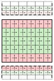
(a)

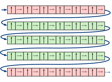
(b)

(c)

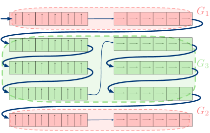
(d)

Figure 1: Illustration of a five-point stencil on a two-component vector field of a 2D Cartesian domain with grid partitioning along one axis (a). As summarized in Table I, the Array-of-Structures (AoS) layout (b) performs only two communications, which is the minimum required to exchange data between partitions. The Structure-of-Arrays (SoA) layout (c) instead ensures coalesced accesses. The disaggregated layout (d) achieves both properties at the same time by ensuring that the data of shared voxels (in red) is stored contiguously.

We argue that additional optimization objectives should be incorporated into the design space of volumetric data structures. While data locality remains a critical factor, we identify opportunities where selectively compromising on locality can lead to improved end-to-end performance by addressing other key objectives. For instance, optimizing multi-GPU communication efficiency by ensuring that transmitted data is laid out contiguously in memory can significantly reduce the number of messages exchanged. Although this approach may decrease data locality for computations within a single GPU, the overall performance benefits from enhanced communication efficiency can outweigh this trade-off (Figure 1).

In this paper, we introduce a method called disaggregated design for volumetric data structures, which seeks to balance multiple performance objectives by:

1. Grouping voxels based on desired properties: Instead of relying solely on spatial locality, we organize voxels according to their most relevant traits, prioritizing key performance objectives.

2. Applying traditional data locality optimizations within voxel groups: Within each group, we leverage data locality wherever possible, ensuring a balance between maintaining locality and addressing other critical performance goals.

We evaluate the performance of the disaggregated design approach on a fluid dynamics solver based on the Lattice Boltzmann Method (LBM) on single- and multi-GPU systems. The achievements of the disaggregated method include:

1. A zero-copy multi-GPU implementation that overlaps computation and communication for dense discretizations, improving scalability by minimizing both the number and size of data transfers. Depending on the domain size, this approach achieves up to a $3\times$ speedup compared to standard state-of-the-art (SOTA) solutions.

2. A disaggregated interface and its associated layout for block-sparse data structures that reduce the impact of high register pressure in complex boundary conditions, e.g., those used in the regularized LBM [12]. This approach achieves up to a $2\times$ speedup compared to a naive implementation while avoiding additional storage overhead for boundary-specific information.

3. A multi-resolution grid representations that maximize kernel fusion in regions of the domain unaffected by neighboring cells of different sizes. This results in up to a 26% performance gain in a single-GPU configuration.

Although we present the disaggregated design method specifically for dense, sparse, and multi-resolution voxel-based representations in this work, the underlying principles are readily applicable to other data structures, e.g., unstructured meshes.

II Disaggregated Design Method

Voxel-based representations, derived from Cartesian discretization, encompass a range of cases. These include the dense representation, where all voxels within a specified multidimensional interval are allocated; the sparse representation, which focuses on a subset of interest (potentially irregular) within the interval; and multi-resolution layouts, where voxels of varying sizes coexist within the same interval. Traditional data structure design has primarily centered on optimizing data locality, as it remains one of the most effective strategies at the software level for addressing the growing gap between computation speed and memory latency in modern architectures.

We recognize that performance-critical optimizations—e.g., minimizing communication overhead, reducing register pressure, and maximizing kernel fusion—are crucial too when designing data structures. To tackle these challenges, we introduce a methodology for the multi-objective design of volumetric data structures, termed disaggregated design, which we define as follows:

Definition 1.

Given an optimization objective $\Phi$ to be considered alongside data locality, a disaggregated design maps data distributed over a voxelized domain into a 1D memory address space through the following four-step process:

1. Definition: Identify a set of properties, $\mathcal{P}_{1},\mathcal{P}_{2},\ldots,\mathcal{P}_{n}$, that influence and improve the optimization objective $\Phi$.

2. Classification: Classify voxels in the domain into groups, $\mathcal{G}_{1},\mathcal{G}_{2},\ldots,\mathcal{G}_{n}$, based on these properties.

3. Mapping: Within each group $\mathcal{G}_{i}$, map voxel data to memory using classical techniques designed to optimize data locality.

4. Operations: Apply specific operations to each group $\mathcal{G}_{i}$ tailored to maximize the optimization objective $\Phi$.

The definition step establishes the design space, enabling a global optimization framework that addresses objectives beyond data locality. This facilitates the classification of voxels into groups, allowing targeted operations to optimize specific objectives. The mapping integrates classical data locality optimizations, albeit confined to a local scope within each group.

Consequently, the effectiveness of the disaggregated design depends on whether the performance gains from optimizing for the objective $\Phi_{i}$ outweigh the inherent limitations of the approach:

• Sub-optimal locality: Data locality may be compromised, as classical optimizations are restricted to the boundaries of individual groups, potentially leaving inter-group locality underutilized.

• Increased complexity: The additional indexing mechanisms required to manage different groups $\mathcal{G}_{i}$ introduce computational overhead and implementation complexity.

To study the applicability and advantages of the disaggregated design in a general context, we focus on a common for-each data-parallel computation pattern where users define a side-effect-free function that is applied independently to each voxel in the domain. Within this model, we analyze three distinct compute patterns:

• Map Pattern: The computation for a voxel depends solely on its local data.

• Uniform Stencil Pattern: The computation for a voxel involves querying data from its neighbors, e.g., in convolution filters or finite difference computations.

• Multi-resolution Stencil Pattern: Multi-resolution discretization extends the uniform Cartesian representation by allowing voxels to have different sizes where voxels fetch information from neighbors at varying resolutions.

In the following, we apply the disaggregated design method to these three compute patterns across dense, sparse, and multi-resolution representations. Sections VI-A and VI-B analyze the performance gains achieved through these optimizations on a fluid simulation solver. The disaggregated definition can naturally be extended to include additional objectives. However, in this study, we focus on a few specific cases where an extra objective is defined alongside data locality.

III Disaggregation on a Dense Domain

In this setup, we consider a dense grid distributed across multiple GPUs, with each GPU responsible for a specific region of the domain. During stencil computations, where data from neighboring voxels is required, one approach involves fetching data directly from neighboring GPUs during each computation step. However, this strategy is highly inefficient due to the substantial communication overhead it incurs.

To address this, a halo region is typically introduced for each partition (Figure LABEL:fig:jacobiParition). Halo regions contain copies of data from adjacent partitions, enabling stencil computations to be performed locally without frequent inter-GPU communication. Maintaining and updating these halo regions introduces its own challenges, as synchronization and communication between GPUs—referred to as the halo update—are required [7]. In a naive implementation [13], the halo update process must be completed before performing the stencil operation. As a result, all time spent on communication directly contributes to the overall execution time.

The Overlapping of Computation and Communication (OCC) optimization addresses this issue by dividing the stencil operation into two phases. The first phase processes private voxels, which can be computed entirely using data stored within a single partition. The second phase handles shared voxels, which rely on data from halo regions updated by neighboring partitions. With OCC, the halo update process is executed in parallel with the computation on private voxels, thereby reducing the direct impact of communication on the overall execution time. This approach is critical for achieving fine-grained parallelism, hiding latency, and improving scalability in multi-GPU systems.

Consider a communication performance model [14] that accounts for a constant setup time ($t_{setup}$) and a time proportional to the size of the transferred message. The latter is defined as the ratio of the message size to the throughput of the interconnect ($b_{com}$):

$$t_{send}(\text{msg})=t_{setup}+\frac{size(\text{msg})}{b_{com}}$$ (1)

This simple model assumes that messages are contiguous in memory. For data mapped to disjoint memory regions, multiple transfers are required to send the information.

On a dense grid, we consider a 2D stencil applied to a vector field, where each point in the Cartesian domain stores a 2D vector. Common memory layouts for representing a partition are Array-of-Structures (AoS) and Structure-of-Arrays (SoA). The SoA layout is generally more efficient on GPUs due to its coalesced memory access pattern [15]. For a grid with dimensions $d_{x}\times d_{y}$, and assuming a 1D partitioning scheme (see Figure LABEL:fig:jacobiParition), the overhead of the halo update for a generic partition can be modeled as:

$$t_{halo\_update}=\alpha t_{setup}+\beta\frac{size(T)}{b_{com}}$$ (2)

Here, $\alpha$ represents the number of transfer operations, while $\beta$ denotes the size of the total number of elements sent to other partitions. In this specific example, the minimum value for $\alpha$ is 2, as each partition in a 1D decomposition has both an upper and a lower neighbor. Meanwhile, $\beta$ corresponds to $2\cdot d_{y}$, representing the number of elements exchanged along the shared boundaries.

With an AoS layout (see Figure LABEL:fig:jacobiAoS), the data for all shared voxels is stored contiguously in memory, ensuring that $\alpha$ achieves its minimum value of 2. However, AoS layouts do not enable coalesced memory access on GPUs, leading to significant performance degradation [15].

Leveraging the SoA layout (Figure LABEL:fig:jacobiSoA) resolves the issue of coalesced memory access. However, it results in a higher $\alpha$ value of 4, as two separate memory transfers are required for each neighboring partition. This increase occurs because the 2D components are stored non-contiguously in memory, as illustrated by the four distinct regions in Figure LABEL:fig:jacobiSoA. To reduce the number of communication operations, the data would need to be copied into a contiguous buffer.

We apply the disaggregated design to minimize $\alpha$, i.e., reducing the number of continuous memory regions used to store shared voxels. In the first step of the disaggregated design, we define $\mathcal{P}_{1}$ and $\mathcal{P}_{2}$ as constraints to enforce a contiguous mapping for data exchanged with the upper and lower partitions, respectively.

Given $\mathcal{P}_{1}$ and $\mathcal{P}_{2}$, the group $\mathcal{G}_{1}$ contains all shared voxels that communicate with the upper partition, $\mathcal{G}_{2}$ includes those communicating with the lower partition, and finally $\mathcal{G}_{3}$ holds the remaining private voxels, as illustrated in Figure LABEL:fig:jacobiDisg. In the second step of the disaggregated design method, we select a SoA layout. By mapping each group separately in memory, the layout preserves the properties $\mathcal{P}_{1}$ and $\mathcal{P}_{2}$.

Table I compares the different memory layouts and demonstrates how the disaggregated method combines the best features of both SoA and AoS. Specifically, it achieves the lowest values for both $\alpha$ and $\beta$ while still supporting coalesced access patterns.

	$\boldsymbol{\alpha}$	$\boldsymbol{\beta}$	Coalesced accesses
AoS	2	$2\cdot d_{x}$	No
SoA	4	$2\cdot d_{x}$	Yes
Disaggregated SoA	2	$2\cdot d_{x}$	Yes

TABLE I: Comparison of the disaggregated layout with AoS and SoA layouts for a five-point stencil operation, based on the model in Eq. 2. The 2D domain has dimensions $d_{x}\times d_{y}$, with 1D partitioning performed along the y-axis.

IV Disaggregation on a Sparse Domain

When the region of interest in a simulation domain is significantly smaller than the full domain, using a dense representation becomes inefficient. In such cases, sparse representations are preferred, as they allocate data only for voxels actively involved in the computation, thereby saving memory and computational costs.

The map pattern is commonly employed in sparse domains, particularly for managing boundary conditions in physics solvers. Listing 1 illustrates a typical scenario, where computations on each voxel depend on its boundary condition type, if any.

For example, in computational fluid dynamics, boundary conditions represent fluid-structure interactions. Walls may enforce no-slip conditions on boundary voxels, while interior non-boundary voxels follow the Navier-Stokes equations.

Function For each voxel(VoxelID):

    // Initial computation on the voxel

    do_initial_computation(VoxelID);

   

   // Determine boundary type

    bc_voxel = get_boundary_condition(VoxelID);

   

   if bc_voxel then

       // Compute boundary conditions

       compute_bc(VoxelID);

      

   // Perform additional computations

    do_final_compute(VoxelID);

   

Algorithm 1 Boundary Conditions Handling

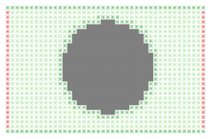
(a)

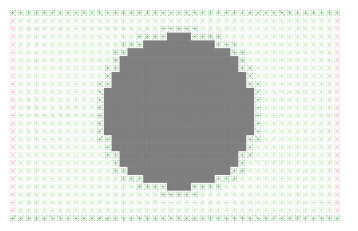
(b)

Figure 2: A typical problem setup for a physics solver, where only a subset of voxels (red) implement complex boundary conditions, while the gray region represents non-computational space. The domain is represented using a block-sparse layout (b), where a block is classified as a boundary block if at least one of its voxels is a boundary voxel.

	# Kernels	# Blocks	# Registers	Storage	Indexing
Naive	1	$n_{b}+n_{nb}$	$r_{b}$	$s_{w}n_{nb}b_{size}$	Direct
Disag - Bitmask	2	$n_{b}+n_{nb}$	$r_{b}$	$s_{i}(n_{b}+n_{nb})b_{size}$	Indirect
		$n_{b}+n_{nb}$	$r_{nb}$
Disag - Mem	2	$n_{b}$	$r_{b}$	$0$	Direct
		$n_{nb}$	$r_{nb}$

TABLE II: Comparison of the disaggregated design against the naive approach for a map pattern involving complex boundary conditions in a block-sparse representation. # Kernels indicates the number of kernels launched. # Blocks represents the number of blocks executed for each kernel. # Registers denotes the number of registers required for each kernel. Storage refers to the memory overhead, where $s_{w}$ is the size of memory required for each boundary voxel, $b_{\text{size}}$ is the number of voxels in a block, and $s_{i}$ is the size of the type selected for indexing.

The ratio of boundary voxels to the total domain is typically proportional to the surface-to-volume ratio of the problem. Consequently, boundary voxels often represent only a small fraction of the domain, as illustrated in Figure 2. In this section, we focus on sparse block representations and assume the use of space-filling curves to optimize memory mapping, although other layouts could also be employed.

The computational load on boundary voxels varies based on their type, introducing several challenges for efficient GPU implementations:

• Register pressure: Boundary condition computations may require additional registers, reducing kernel occupancy and potentially causing register spilling.

• Memory overhead: Managing boundary conditions often requires per-voxel metadata, increasing memory requirements.

To model resource usage, we define $r_{\text{nb}}$ as the resources required for non-boundary computations and $r_{\text{b}}$ for boundary computations. We focus the subsequent discussion, in more common and difficult scenarios where $r_{\text{b}}>r_{\text{nb}}$, resulting in performance degradation due to reduced occupancy or increased memory overhead.

IV-A Naive Approach

A naive approach executes a single GPU kernel across all voxels, with both core computations and boundary condition logic compiled into it. The resource usage is expressed as:

$$r=\max(r_{\text{nb}},r_{\text{b}})=r_{\text{b}}.$$ (3)

Although the majority of voxels require only $r_{\text{nb}}$ resources, the kernel is constrained by the higher resource demands of the boundary voxels ($r_{\text{b}}$). For example, managing complex boundary conditions may significantly increase the kernel’s register usage, leading to reduced occupancy and inefficient GPU utilization. Similarly, memory allocation in naive implementations typically follows a full buffer allocation strategy, where memory is allocated for the entire domain, even though boundary voxels occupy only a small fraction of the total space.

IV-B Disaggregated Approach

Sparse domains often exhibit heterogeneous workloads, where boundary voxels require significantly more resources than non-boundary voxels. By leveraging a disaggregated design, computations and memory layouts can be tailored to the specific needs of each group, mitigating inefficiencies inherent in traditional approaches.

Unlike the naive approach, which launches a single kernel constrained by $r_{\text{b}}$, the disaggregated approach divides the domain into two distinct groups:

• Boundary Group ($\mathcal{G}_{\text{b}}$): Blocks containing at least one boundary voxel.

• Non-Boundary Group ($\mathcal{G}_{\text{nb}}$): Blocks containing only non-boundary voxels.

This separation allows two specialized kernels to operate independently: one for boundary voxels and another for non-boundary voxels. We consider two implementations of this concept:

Memory-Based Grouping

In this implementation, boundary blocks are reordered to appear contiguously in memory, followed by non-boundary blocks. Two kernels are then launched to process their respective groups, eliminating the need for runtime checks at the block level. This static grouping simplifies memory access patterns and removes the overhead associated with indirect indexing.

Bitmask-Based Grouping

In this implementation, we use a bitmask at runtime to distinguish block types. Since the spans of the two groups are no longer contiguous, both kernels must execute over the entire domain. Memory for boundary-specific data is allocated using indirect indexing, where a unique identifier is assigned to each voxel. This identifier maps boundary voxels to their metadata, which is stored in a contiguous buffer.

Table II summarizes the properties of these three approaches. In Section VI-B, we analyze the performance and trade-offs of each implementation in detail.

V Disaggregation on a Multi-resolution Domain

(a)

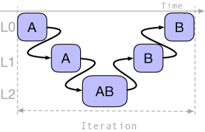
(b)

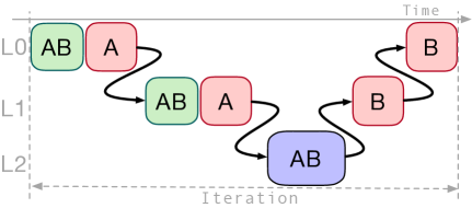
(c)

Figure 3: A multi-resolution domain with three levels (a) where red blocks are near resolution jumps, and green blocks are farther away. The computational graph (b) illustrates the dependencies between kernels: both kernel A and kernel B run on red and green blocks, but kernel B must wait for boundary information to be resolved. Since no boundaries exist at the finest level, kernels A and B can only be fused at that level. In the disaggregated approach (c), kernels can be fused at any level for green blocks, while red blocks requiring boundary resolution execute the two kernels sequentially after boundary information is resolved, reducing iteration time and improving efficiency.

Multi-resolution data structures manage voxels of varying sizes within the same domain (Figure 3) and provide mechanisms to support map operations, as well as stencil operations both within a resolution level (intra-level operations) and across adjacent resolution levels (cross-level operations).

In time discretization for multi-resolution scenarios [16], only voxels near a resolution jump participate in cross-level interactions during a solver iteration. Figure 3 highlights this distinction: green voxels represent regions of intra-level operations, while red voxels indicate regions affected by cross-level dependencies. Due to the producer/consumer relationship between resolution levels, iterations are traditionally split into two steps, which can only be fused at the finest resolution level, as illustrated in Figure LABEL:fig:mres:naive.

Using the disaggregated design, we improve memory throughput by maximizing kernel fusion opportunities for intra-level computations. Our approach leverages the observation that voxels far from resolution jumps do not require cross-level communication, allowing their iterations to be fused naturally at any resolution level. To formalize this, we introduce a discrete distance property, $\mathcal{P}_{d}$, which measures the distance of a voxel from a resolution jump, where a distance of zero indicates direct proximity to the jump. Based on this property, we classify blocks at each resolution level into two groups:

1. $\mathcal{G}_{\text{i}}$: Blocks where all voxels have a distance of one or greater from a resolution jump, allowing fully fused intra-level operations.

2. $\mathcal{G}_{\text{c}}$: Blocks containing at least one voxel with a distance of zero, requiring separate cross-level and intra-level computations.

We apply a standard memory locality layout to map each group within the block representation for each resolution level. In the disaggregated design, different kernels are executed for the two groups. For $\mathcal{G}_{\text{i}}$, computations are fully fused across resolution levels, enabling optimized kernel execution. In contrast, computations for $\mathcal{G}_{\text{c}}$ are delayed until boundary information becomes available, as shown in Figure LABEL:fig:mres:disg, which illustrates this for a three-level grid. The primary optimization objective of this approach is to reduce memory pressure by enabling efficient fused operations for $\mathcal{G}_{\text{i}}$, while ensuring accurate cross-level computations for $\mathcal{G}_{\text{c}}$.

VI Evaluation and Discussions

In this section, we will analyze the disaggregated design method by analyzing a fluid dynamics simulation application based on LBM on a dense, sparse, and multi-resolution grid. Emerging as a reliable, computationally efficient, and scalable alternative to conventional Navier-Stokes solvers, LBM is increasingly used for numerical simulation of complex engineering and environmental flows [17]. We pick LBM as a representative application since it could benefit from many of the objectives our design method targets.

The LBM describes the time evolution of a collection of fictitious particles, represented by time-dependent velocity distribution functions ($f_{i}$) along a set of discrete lattice directions, denoted by $e_{i}=(e_{1},\ldots,e_{q})$. We refer to $f_{i}$ as the populations. We employ 3D lattice structures with 19 (D3Q19) and 27 (D3Q27) directions. The values of $f_{i}$ are updated over time using a collide-and-stream algorithm, which consists of two key steps:

Collision: $$f_{i}^{\ast}(x,t)=\mathcal{C}(f_{i}(x,t))$$ (4)

Streaming: $$f_{i}(x+e_{i}\Delta x,t+\Delta t)=f_{i}^{\ast}(x,t)$$ (5)

The collision operation, $\mathcal{C}$, is a nonlinear and computationally local operation that modifies $f_{i}$ at a given lattice point. The fluid density, velocity, and pressure can then be derived from these distribution functions. We employ the single-relaxation-time collision model of Bhatnagar-Gross-Krook (BGK) [18] for this step. While the collision and boundary operations for each individual $f_{i}$ are typically local, the streaming operation is non-local—it advects $f_{i}$ in space by shifting information along each of the $Q$ discrete directions using a stencil operation. This spatial dependency introduces a key computational challenge in LBM, as it requires efficient handling of data movement across the lattice. In optimized LBM implementation on GPU, an entire iteration (collision, streaming, and boundary conditions) is fused into a single kernel [19].

We based our reference implementation on the work of Meneghin et al. [7], which achieved state-of-the-art performance for both single- and multi-GPU implementations. Our baseline performance aligns with their results. We also validate our implementation against empirical data (see Appendix -A).

VI-A Improving LBM Scalability

Using a lid-driven cavity flow problem modeled with LBM [20] on a cubic domain, we evaluate the scalability of our disaggregated design approach in single-node multi-GPU systems using a dense voxel representation. The analysis is based on a theoretical model following the formalism introduced in Section III, and an assessment of runtime performance.

VI-A1 Reference Implementation

In single-node multi-GPU systems, communication can be performed via PCI or specialized interconnects like Nvidia’s NVLink. While major MPI implementations (e.g., CUDA-aware MPI) are designed to leverage the best available interconnects, we utilize native communication mechanisms (cudaMemcpyPeer) exclusively, as they have demonstrated superior performance [21].

These systems typically support up to 8–16 GPUs, making 1D partitioning a practical choice over more complex 2D or 3D partitioning schemes [22]. With 1D partitioning, each partition has at most two neighbors, providing two key benefits: 1) a reduction in the number of communications required, and 2) compatibility with the linear memory topology, enabling efficient zero-copy memory transfers.

Figure LABEL:fig:partitionHalo illustrates the data dependencies between partitions imposed by the LBM streaming operator. Private voxels’ (highlighted in green) computations depend only on GPU-local data. Shared voxels (highlighted in red) require data from either the upper or lower neighboring partition. At the lattice granularity, some populations are local to the partition (white or gray populations inside grid cells), whereas others must be exchanged between partitions (colored populations). Specifically, red populations must be retrieved from the upper neighboring partition, and blue populations must be retrieved from the lower partition. Importantly, only a subset of a shared voxel’s population needs to be exchanged, which is a defining feature of the LBM streaming operation.

Efficient OCC is critical for achieving fine-grain scalability in LBM [7]. Figure LABEL:fig:occGraph illustrates the execution graph of an iteration using OCC, where computations on private voxels are overlapped with the communications required to resolve remote data dependencies for shared voxels. By overlapping these operations, communication latency is effectively hidden, resulting in improved overall performance and scalability. We refer to this approach as the reference implementation.

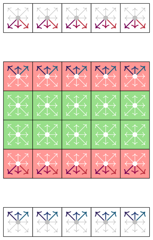
(a)

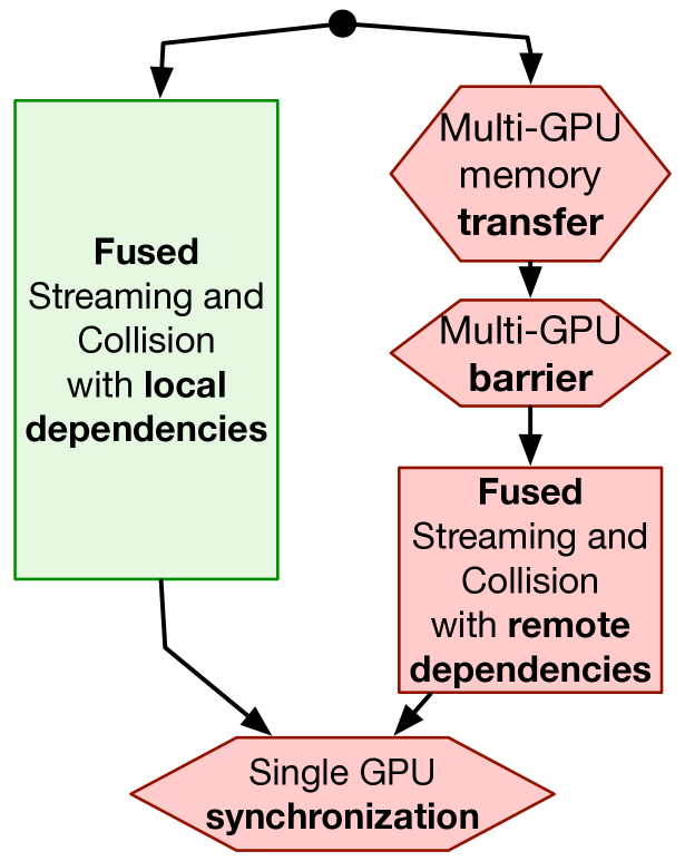
(b)

Figure 4: LBM grid with 1D partitioning (a) where white arrows indicate GPU-local dependencies, while blue and red arrows represent remote dependencies to the upper and lower partitions, respectively. The reference implementation employs OCC as depicted in the execution graph (b).

	D2Q9		D3Q19		D3Q27
	$\alpha$	$\beta$	$\alpha$	$\beta$	$\alpha$	$\beta$
AoS	2	18s	2	38s	2	54s
SoA	6	6s	10	10s	18	18s
Disaggregated SoA	2	6s	2	10s	2	18s

TABLE III: Modeling of the LBM communication overhead with respect to Eq. 2. $s$ represents half of the partition’s shared voxels: $d_{x}$ for the 2D case and $d_{x}\cdot d_{y}$ for the 3D case.

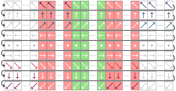
(a)

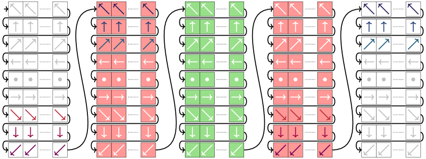
(b)

Figure 5: Representation of SoA and disaggregated SoA layouts of a dense domain for a D2Q9 LBM lattice. The color semantics follow those presented in Figure LABEL:fig:partitionHalo. The black arrows specify how the elements are mapped to memory.

VI-A2 Modeling Communication Overhead

For LBM, the parameters $\alpha$ and $\beta$ in Eq. 2 depend on both the type of LBM lattice and the data layout (Table III). As for the stencil operations on a vector field, the populations can be arranged according to AoS or SoA.

Considering a D2Q9 case with an AoS layout, the populations are stored contiguously for each voxel. To send the information to the upper partition, we can execute a transfer operation per voxel, which is not feasible as it would require too many transfers, i.e., the value of $\alpha$ would depend on the domain size. Alternatively, we can execute only one transfer exporting the entire voxel information which is more than what is needed to satisfy data dependencies, i.e., we increase $\beta$ to constrain the value of $\alpha$. For such a case, $\alpha$ is equal to two (a send operation per neighbor) and $\beta$ is equal to $18s$; $s$ is the number of shared voxels per neighboring partition.

For the D2Q9 with SoA case, we use Figure LABEL:fig:soaLayout to identify the parameter values. The populations that need to be transferred are represented by blue or red arrows, and they are stored continuously per direction. Therefore, we execute 9 send operations per neighbor, and we transfer the minimum amount of data required, which gives us a value of 6 for both $\alpha$ and $\beta$. Table III summarizes the model values, including D3Q19 and D3Q27. AoS has the lower value of $\alpha$ but also the higher value of $\beta$.

VI-A3 Disaggregated Optimization

In the following, we extend the disaggregated layout previously defined for stencil operations on a vector-valued field example. To fully support a zero-copy communication approach, we include halo regions. The defined properties ensure continuity for the following regions: upper halos, upper boundary voxels, lower boundary voxels, and lower halos. Each group is still mapped using an SoA layout. Figure LABEL:fig:disComLayout illustrates both the grouping and the resulting memory mapping. In this layout, any data that needs to be transferred or received is mapped contiguously in memory. This property is visually evident in Figure LABEL:fig:disComLayout, where populations of the same color (red or blue) are arranged continuously in memory. For the D2Q9 example, the disaggregated SoA layout achieves an $\alpha$ value of 2 (each partition sends only one message per neighboring partition) and a $\beta$ value of 6 (representing the minimum amount of data exchanged). Table III reports the $\alpha$ and $\beta$ values for the D3Q19 and D3Q27 lattices, confirming that the disaggregated layout consistently offers the best results. This layout combines the advantages of both AoS and SoA designs. It achieves the minimal number of send operations, comparable to AoS, while also minimizing the data transferred, as in SoA. It also maintains zero-copy efficiency, making it theoretically the most communication-efficient approach by minimizing overhead.

VI-A4 Benchmarking

While the performance model highlighted the positive impact of a disaggregated layout (Section III), runtime analysis is necessary to determine whether the intrinsic overheads introduced by the disaggregated approach (discussed in Section II) are justified by the overall performance improvements. For this evaluation, we focus on the lid-driven cavity flow problem on a cubic domain—a well-established benchmark in the computational fluid dynamics community. The boundary condition setup and problem implementation follow the work of Latt et al. [20].

We consider three single-node multi-GPU systems based on Nvidia architectures, as detailed in Table IV. The A100 serves as a high-end server-grade solution tailored for HPC and AI workloads, while the A10 provides a more affordable option designed primarily for graphics tasks. The V100, in contrast, represents the previous generation of Nvidia GPUs. Both the A100 and V100 systems leverage Nvidia’s high-speed NVLink interconnect for fast GPU-to-GPU communication.

Name	Architecture	GPUs	Memory	Interc.
DGX-A100	A100-SXM4	8	40GB	Nvlink-2
AWS p3	V100-SXM2	8	16GB	Nvlink-1
AWS g5	A10	8	24GB	PCI

TABLE IV: List of machines used for benchmarking.

In our benchmarks, we exclude AoS configurations due to their significantly lower performance for LBM, which is attributed to non-coalesced memory accesses. We focus on 3D domains utilizing D3Q19 and D3Q27 lattices, tested with both single and double precision data types (Figure 6 and Appendix -B). Solver throughput is evaluated using the Million Lattice Updates Per Second (MLUPS) metric.

(a)

Figure 6: Comparison of MLUPS performance between the disaggregated design (Disag) and SoA on the lid-driven cavity flow problem using D3Q19 lattices on 8 GPUs in a cubic domain.

The disaggregated layout consistently outperforms or matches the SoA layout across all configurations, delivering particularly notable performance gains for small to medium domain sizes. For domains smaller than $150^{3}$, the disaggregated layout achieves up to a $4\times$ speedup. For domains between $150^{3}$ and $250^{3}$, it provides a $2.5\times$ speedup. For larger domains, the performance gains taper to approximately $1.5\times$. This reduction in performance improvement for larger domains is well explained by Eq. 2: under a 1D partitioning strategy, the impact of $\beta$ (the amount of data transferred) increases with domain size. Meanwhile, the number of private voxels grows cubically with the domain edge length $L$, significantly increasing the amount of computation that can be overlapped with communication.

A similar pattern is observed when comparing single and double precision. Double precision increases $\beta$ due to the larger data size while maintaining the same $\alpha$ for a given lattice. However, it also makes computations more resource-intensive, creating additional opportunities to overlap computation with communication. This overlap mitigates the performance degradation caused by increased data transfer, ensuring the efficiency of the disaggregated layout.

The comparison between D3Q19 and D3Q27 lattices (see Appendix -B) reveals that the performance advantages of the disaggregated layout become more pronounced with lattices that feature a larger number of populations. This trend aligns with Eq. 2, as the difference in $\alpha$ values between the native and disaggregated layouts increases for D3Q27, driven by its higher population count.

To further illustrate scalability, Figure 7 presents a strong scaling plot for domains of size $192^{3}$ (additional results can be found in the Appendix -B). The plot highlights the effectiveness of the disaggregated approach across different levels of fine-grain parallelism. Traditional methods struggle to scale efficiently for these domain sizes, typically achieving a maximum speedup of around $3\times$ relative to single GPU execution. In contrast, the disaggregated layout consistently delivers scalability improvements of $6\times$ or more, regardless of the GPU architecture used.

Figure 7: Strong scaling of the LBM lid-driven cavity flow on a single-node multi-GPU system for a domain size of $192^{3}$, using a single precision D3Q27 lattice.

VI-B Improving LBM Register Allocation

To assess the impact of the disaggregated design on register allocation, we analyze an application simulating fluid flow over an obstacle in a cubic domain using LBM. The fluid domain is modeled using a block-sparse grid with fixed block sizes, where each block contains $4^{3}$ voxels. This setup represents a typical wind tunnel problem, where the bounce-back boundary condition [23] is applied to the surfaces of the obstacle and four faces of the cubic domain. Additionally, an inflow boundary condition is applied to one face to simulate the inlet flow, and an outflow boundary condition is applied to the opposite face for the outlet flow. Figure 2 provides a 2D illustration of this setup, with light green voxels representing internal fluid that requires no boundary conditions, dark green voxels marking bounce-back boundary condition regions, and red voxels for inflow and outflow regions.

The bounce-back boundary condition is a register-light method, requiring only $2Q$ populations—the same number used during the collide-and-stream steps, where $Q$ represents the lattice size of the LBM scheme. For voxels subject to boundary conditions, an LBM iteration typically consists of three steps that are often fused into a single kernel: 1) streaming, 2) boundary condition treatment, and 3) collision.

The bounce-back condition is highly efficient in terms of register usage, as its resource requirements closely match those of the stream and collision steps in standard LBM computations. In contrast, the inflow and outflow boundaries on opposite faces of the domain utilize the regularized boundary condition [24]. This method is register-heavy, requiring $3Q$ populations to represent the LBM state. A kernel that combines both boundary conditions—bounce-back and regularized—would need virtual registers proportional to $r>\max(3Q,2Q)$. This leads to increased register allocation and potential reduced kernel occupancy, especially since the proportion of regularized voxels relative to the total number of voxels decreases inversely with the domain size, $\mathcal{O}\left(\frac{1}{x}\right)$, where $x$ is the edge length of the domain. Thus, a naive implementation would result in over-allocation of registers for most of the domain, where such high resource usage is unnecessary.

To address this inefficiency, we apply the disaggregated design methodology, grouping voxels based on their register requirements. Voxels requiring the regularized method are assigned to the boundary group, while the remaining voxels, including bounce-back voxels, fall into the non-boundary group. For the rest of this section, the term boundary will exclusively refer to the regularized case. Consequently, blocks containing at least one boundary voxel are classified as boundary blocks, while the remaining blocks are classified as non-boundary blocks.

By either mapping boundary blocks contiguously in memory or using a bitmask to distinguish boundary from non-boundary blocks, the disaggregated approach ensures that kernels for non-boundary blocks operate with reduced register pressure, maximizing occupancy and execution efficiency. Analytically, this solution aligns with the theoretical advantages outlined in Table II, highlighting the efficacy of the disaggregated design in mitigating register-related bottlenecks.

Figure 8: Comparison of the performance between the baseline and our disaggregated design for flow over an obstacle on a single GPU, using a block-sparse grid with a D3Q27 lattice in single precision. Inflow and outflow boundary conditions are regularized boundary condition [24].

VI-B1 Benchmarks

We ran the application on a single GPU from the systems listed in Table IV, using CUDA compiler heuristics to determine the number of registers required and the amount of data to spill into the GPU’s local memory when necessary. Figure 8 presents the performance results of D3Q27 lattices in single precision across varying domain sizes (D3Q19 results are reported in Appendix -C). Across all GPUs and domain sizes, the disaggregated solutions (using either the bitmask or continuous block allocation approaches) consistently outperform the naive approach. Performance gains can exceed $2\times$, particularly on the V100 and A10 GPUs. On the A100, the maximum observed gain is capped at $1.3\times$. While the differences between the two disaggregated solutions are minimal, the continuous block allocation approach shows a slight advantage over the bitmask solution for larger domains, with gains of up to 6%.

The higher performance boost on the V100 is due to the naive kernel’s usage of 55 registers, the same number used by the boundary kernels in the disaggregated solutions. With 55 registers, registers spilling happens to the local memory which affects the naive approach for processing the whole domain. With the disaggregated approach, this kernel will only run on the boundary blocks while representing a small portion of the whole domain while the rest of the domain is processed via a more efficient kernel, i.e., non-boundary kernel. For a domain size of 368, the naive kernel experiences $2.2\times$ higher data traffic between L2 and DRAM, leading to the observed $2\times$ performance boost with the disaggregated solutions.

On the A100, all compiled kernels (naive and disaggregated) use 55 registers, and register spilling again occurs only with the naive method. However, the A100’s larger L2 cache mitigates the impact of spilling, resulting in reduced performance penalties for the naive approach compared to the V100 GPU. The naive kernel still incurs $1.3\times$ higher data traffic between L2 and DRAM compared to the disaggregated method, corresponding to the $1.3\times$ MLUPS speedup achieved with the disaggregated solution on the A100 GPU.

For the additional memory required to handle boundary conditions, the regularized method for a velocity profile stores a vector with $d$ components (2 in 2D and 3 in 3D). Therefore, given $F$ as the type used to represent velocity and $I$ as the type used for indexing, the memory requirements are calculated as follows: $s_{w}=\text{sizeOf}(F)\cdot d$ and $s_{i}=\text{sizeOf}(I)$. The disaggregated method remains the only approach that does not require any extra storage (see Table II).

VI-C Improving Multi-resolution LBM Kernel Fusion

GPU	Domain Size	Distribution	Ours	Baseline	Gain
A100	$512^{3}$	77, 4, 0.4	6072	4824	25%
A100	$512^{3}$	73, 3, 0.5, 0.003	6018	4769	26%
V100	$320^{3}$	15, 1, 0.1	4421	3770	17%
V100	$320^{3}$	15, 1, 0.1, 0.002	4422	3770	17%
V100	$480^{3}$	53, 4, 0.4	5006	4047	23%
V100	$480^{3}$	53, 4, 0.3, 0.008	5005	4050	23%
A10	$320^{3}$	15, 1, 0.1, 0.002	4083	3982	2%
A10	$480^{3}$	53, 4, 0.3, 0.008	4483	4306	4%
A10	$512^{3}$	77, 4, 0.4	4093	3901	4%
A10	$512^{3}$	73, 3, 0.5, 0.003	3890	3719	4%

TABLE V: Comparing the performance of the baseline algorithm grid refinement LBM to our disaggregated implementation using an example lid-driven cavity flow with three and four levels of grid refinement in single precision. Size indicates the length of the virtual box described in the finest level along $x$, $y$, and $z$ directions; Distribution indicates the distribution of active voxels across different levels starting from the finest level; Baseline refers to the MLUPS achieved by the baseline algorithm [25]; Ours refers to our implementation; and Gain = (Ours-Baseline)/Baseline $\times$ 100%.

We tested the disaggregated approach on a single-GPU-optimized multi-resolution LBM algorithm, as described by Mahmoud et al. [25]. The data structure consists of a stack of uniform block-sparse grids, one for each resolution level, along with metadata to manage transitions between levels.

In the context of multi-resolution LBM, the algorithm introduces inter-level data dependencies during execution. These dependencies manifest in two distinct ways:

• Explosion: Collision data at a given resolution level is used by lower resolution levels, propagating information downward in the hierarchy.

• Coalescence: Streaming data is consumed from higher resolution levels, aggregating information upward in the hierarchy.

These dependencies create a dependency graph similar to the one presented in Figure LABEL:fig:mres:naive, where operator A represents collision, and operator B represents streaming. At all resolution levels except the finest, these dependencies prevent kernel fusion, as explosion and coalescence require intermediate data to be available between operations.

Since only voxels near resolution transitions (jumps) are affected by these inter-level dependencies, we classify blocks into two categories:

• $\mathcal{P}_{\text{uniform}}$: Blocks that execute the LBM algorithm in a uniform manner without requiring explosion or coalescence.

• $\mathcal{P}_{\text{jump}}$: Blocks where explosion and coalescence dependencies must be explicitly managed for at least one voxel.

Using the disaggregated interface, we reorganize the multi-resolution execution graph by eliminating unnecessary dependencies due to kernel granularity. For blocks in $\mathcal{P}_{\text{uniform}}$, we execute a fused version of the LBM kernel, leveraging the absence of inter-level dependencies to improve efficiency. For blocks in $\mathcal{P}_{\text{jump}}$, we maintain the original execution graph to handle explosion and coalescence correctly.

Table V summarizes the performance comparison between our disaggregated implementation and the optimized baseline algorithm [25] for the lid-driven cavity flow problem, using single precision across different GPUs and domain sizes. The results demonstrate that the disaggregated approach consistently outperforms the baseline, with performance gains varying across GPU architectures and problem configurations. On the A100 GPU, which represents a high-end architecture, the disaggregated solution achieves up to a 26% improvement for a $512^{3}$ domain. The V100 GPU also shows substantial gains, with up to 23% improvement for domains of $480^{3}$. These gains are attributed to the efficient handling of explosion and coalescence dependencies through the disaggregated design, which enables kernel fusion for uniform blocks while maintaining the original execution graph for jump blocks.

In contrast, the A10 GPU, designed for less demanding workloads, exhibits more modest performance improvements, with gains ranging from 2% to 4%. This is due to spilling, which has a greater impact on the A10 due to its reduced cache sizes and slower memory bandwidth compared to the A100, despite being based on the same architecture. Overall, the results highlight the effectiveness of the disaggregated design in leveraging different GPU architectures, with the largest benefits observed for larger domains with more active voxels across multiple levels of grid refinement.

VII Related Work

While extensive research has been conducted on optimizing stencil computations, most efforts focus on improving data locality. To the best of our knowledge, this work is the first to propose a data structure design methodology aimed at multi-objective optimization, where data locality can be strategically traded off for other performance goals.

Optimizing communications via data layout: Zhao et al. [26] introduced a layout scheme for block representations designed to minimize communication overhead and enable zero-copy communication. Their approach incorporates virtual memory techniques to reduce the impact of indirect indexing which is effective for stencils with a radius that is a multiple of four. However, for stencils with a radius of one, users must resort to time tiling, which can increase message sizes or become infeasible if reductions are involved. While their method demonstrates significant speedups on distributed systems, it does not address the challenges of multi-cardinality fields.

Reducing Register Pressure and Spilling: Managing register pressure and minimizing spilling are critical challenges in GPU computing. Temporal blocking techniques, e.g., register blocking, serialize one domain dimension to improve data reuse [27]. Other strategies leverage GPU shared memory to mitigate the impact of spilling [28]. However, no prior work has explored using data structure design to address register pressure, especially for complex boundary conditions.

Kernel Fusion: Kernel fusion is a well-known optimization for memory-bound problems, as it reduces memory pressure by keeping shared data in registers between consecutive kernels. This technique is widely used in dense LBM implementations [20] and multi-resolution representations [29]. However, existing works do not explore leveraging data layouts to facilitate kernel fusion.

VIII Conclusion and Future Works

Prior research on volumetric computation has enabled data structure designers to define new layouts that maximize performance, primarily by improving memory access patterns. In this paper, we introduced the disaggregated design approach, a unified framework that expands the scope of performance optimizations to address a broader range of objectives, including reducing multi-GPU memory transfers, minimizing register pressure, and maximizing kernel fusion. Through analytical and empirical evaluation, we demonstrated the advantages of these optimizations while also addressing potential trade-offs. Although the resulting data structures may involve more complex indexing schemes and could compromise memory locality, their overall effectiveness depends on whether the performance gains outweigh these limitations.

This work represents the first comprehensive analysis of the disaggregated design approach and its applicability. It also opens the door for future research in several key directions. First, extending the applicability of the disaggregated design to other spatial data structures, e.g., unstructured meshes, hash grids, and tree-based structures. Second, exploring additional optimization objectives tailored to diverse computational workloads, e.g., enhancing load balancing for particle-based simulations and improving efficiency in distributed systems. Finally, investigating the composability of these solutions—how they can integrate seamlessly with existing frameworks and workflows—represents another important avenue for future exploration.

-A Validation

Figure 9: LBM lid-driven cavity flow validation.

We validated our simulation using the canonical lid-driven cavity flow against the accepted reference data of Ghia et al. [30] where we sampled the domain along $x$ and $y$ axes that run through the center of the domain. Figure 9 shows that our results are well-aligned with the reference data.

-B Improving LBM Scalability - Additional Data

We provide additional scalability data for the LBM disaggregated design discussed in Section VI-A. Figure 12 shows the LBM throughput for a D3Q27 lattice in both single and double precision, as well as the performance for D3Q19 in double precision. Additionally, Figure 10 shows the strong scaling of a D3Q27 lattice in single precision on a $208^{3}$ cubic domain.

Figure 10: Strong scaling of the LBM lid-driven cavity flow on a single-node multi-GPU system for a domain size of $208^{3}$, using a single precision D3Q27 lattice.

-C Improving LBM Register Allocation - Additional Data

We provide additional performance data for the LBM disaggregated design discussed in Section VI-B using a block-sparse representation. Figure 11 presents the single-GPU throughput for a D3Q19 lattice in single precision.

Figure 11: Comparison of the performance between the baseline and our disaggregated design for flow over an obstacle on a single GPU, using a block-sparse grid with a D3Q19 lattice in single precision. Inflow and outflow boundary conditions are regularized boundary condition [24].

(a)

(b)

(c)

Figure 12: Lid-driven cavity flow MLUPS performance for D3Q19 and D3Q27 lattices on 8 GPUs in a cubic domain, with grid resolution specified by the domain’s edge length.

References

- [1] W. A. Wulf and S. A. McKee, “Hitting the memory wall: implications of the obvious,” ACM SIGARCH Computer Architecture News, vol. 23, no. 1, pp. 20–24, Mar. 1995.
- [2] K. Asanovic, R. Bodik, J. Demmel, T. Keaveny, K. Keutzer, J. Kubiatowicz, N. Morgan, D. Patterson, K. Sen, J. Wawrzynek, D. Wessel, and K. Yelick, “A view of the parallel computing landscape,” Communications of the ACM, vol. 52, no. 10, pp. 56–67, Oct. 2009.
- [3] T. Endo, “Applying recursive temporal blocking for stencil computations to deeper memory hierarchy,” in 2018 IEEE 7th Non-Volatile Memory Systems and Applications Symposium (NVMSA). IEEE, 2018, pp. 19–24.
- [4] D. Wonnacott, “Using time skewing to eliminate idle time due to memory bandwidth and network limitations,” in Proceedings 14th International Parallel and Distributed Processing Symposium., ser. IPDPS 2000, May 2000, pp. 171–180.
- [5] U. Bondhugula, A. Hartono, J. Ramanujam, and P. Sadayappan, “A practical automatic polyhedral parallelizer and locality optimizer,” in Proceedings of the 29th ACM SIGPLAN Conference on Programming Language Design and Implementation, 2008, pp. 101–113.
- [6] M. Frigo, C. E. Leiserson, H. Prokop, and S. Ramachandran, “Cache-oblivious algorithms,” in 40th Annual Symposium on Foundations of Computer Science (Cat. No. 99CB37039). IEEE, 1999, pp. 285–297.
- [7] M. Meneghin, A. H. Mahmoud, P. K. Jayaraman, and N. J. W. Morris, “Neon: A multi-GPU programming model for grid-based computations,” in Proceedings of the 36th IEEE International Parallel and Distributed Processing Symposium, Jun. 2022, pp. 817–827. [Online]. Available: https://escholarship.org/uc/item/9fz7k633
- [8] D. Wonnacott, “Using time skewing to eliminate idle time due to memory bandwidth and network limitations,” in Proceedings 14th International Parallel and Distributed Processing Symposium. IPDPS 2000. IEEE, 2000, pp. 171–180.
- [9] X. Wang, Y. Qiu, S. R. Slattery, Y. Fang, M. Li, S.-C. Zhu, Y. Zhu, M. Tang, D. Manocha, and C. Jiang, “A massively parallel and scalable multi-GPU material point method,” ACM Trans. Graph., vol. 39, no. 4, Aug. 2020.
- [10] N.-P. Tran, M. Lee, and S. Hong, “Performance optimization of 3d lattice Boltzmann flow solver on a GPU,” Scientific Programming, vol. 2017, no. 1, Jan. 2017.
- [11] A. B. Hayes, L. Li, D. Chavarría-Miranda, S. L. Song, and E. Z. Zhang, “Orion: A framework for gpu occupancy tuning,” in Proceedings of the 17th International Middleware Conference, ser. Middleware ’16. New York, NY, USA: Association for Computing Machinery, Nov. 2016.
- [12] J. Latt, B. Chopard, O. Malaspinas, M. Deville, and A. Michler, “Straight velocity boundaries in the lattice Boltzmann method,” Physical Review E, vol. 77, no. 5, p. 056703, 2008.
- [13] W.-m. W. Hwu, D. B. Kirk, and I. El Hajj, Programming Massively Parallel Processors: A Hands-on Approach, 1st ed. San Francisco, CA, USA: Morgan Kaufmann Publishers Inc., 2023.
- [14] D. Culler, R. Karp, D. Patterson, A. Sahay, K. E. Schauser, E. Santos, R. Subramonian, and T. von Eicken, “LogP: towards a realistic model of parallel computation,” in Proceedings of the Fourth ACM SIGPLAN Symposium on Principles and Practice of Parallel Programming, ser. PPOPP ’93. New York, NY, USA: Association for Computing Machinery, Jul. 1993, pp. 1–12.
- [15] M. Wittmann, T. Zeiser, G. Hager, and G. Wellein, “Comparison of different propagation steps for lattice Boltzmann methods,” Comput. Math. Appl., vol. 65, no. 6, pp. 924–935, Mar. 2013.
- [16] D. Lagrava, O. Malaspinas, J. Latt, and B. Chopard, “Advances in multi-domain lattice Boltzmann grid refinement,” Journal of Computational Physics, vol. 231, pp. 4808–4822, may 2012.
- [17] C. K. Aidun and J. R. Clausen, “Lattice-boltzmann method for complex flows,” Annual review of fluid mechanics, vol. 42, pp. 439–472, 2010.
- [18] T. Krüger, H. Kusumaatmaja, A. Kuzmin, O. Shardt, G. Silva, and E. M. Viggen, The Lattice Boltzmann method, 1st ed. Springer Cham, 2016.
- [19] M. Geier and M. Schönherr, “Esoteric Twist: An efficient in-place streaming algorithmus for the lattice boltzmann method on massively parallel hardware,” Computation, vol. 5, no. 2, p. 19, Mar. 2017.
- [20] J. Latt, C. Coreixas, and J. Beny, “Cross-platform programming model for many-core lattice Boltzmann simulations,” PLOS ONE, vol. 16, no. 4, pp. 1–29, 04 2021.
- [21] J. Kraus. Multi-GPU programming models. Nvidia. [Online]. Available: https://www.nvidia.com/en-us/on-demand/session/gtcfall21-a31140/
- [22] B. Wilkinson and M. Allen, Parallel programming: techniques and applications using networked workstations and parallel computers, 2nd ed. USA: Prentice-Hall, Inc., Jan. 2004.
- [23] P. Lavallée, J. P. Boon, and A. Noullez, “Boundaries in lattice gas flows,” Physica D: Nonlinear Phenomena, vol. 47, no. 1, pp. 233–240, 1991. [Online]. Available: https://www.sciencedirect.com/science/article/pii/016727899190294J
- [24] J. Latt, B. Chopard, O. Malaspinas, M. Deville, and A. Michler, “Straight velocity boundaries in the lattice Boltzmann method,” Physical Review E, vol. 77, no. 5, May 2008.
- [25] A. H. Mahmoud, H. Salehipour, and M. Meneghin, “Optimized GPU implementation of grid refinement in lattice Boltzmann method,” in Proceedings of the 38th IEEE International Parallel and Distributed Processing Symposium, Jul. 2024, pp. 398–407. [Online]. Available: http://escholarship.org/uc/item/0x86w4w1
- [26] T. Zhao, M. Hall, H. Johansen, and S. Williams, “Improving communication by optimizing on-node data movement with data layout,” in Proceedings of the 26th ACM SIGPLAN Symposium on Principles and Practice of Parallel Programming, ser. PPoPP ’21. New York, NY, USA: Association for Computing Machinery, 2021, pp. 304–317.
- [27] K. Matsumura, H. R. Zohouri, M. Wahib, T. Endo, and S. Matsuoka, “AN5D: automated stencil framework for high-degree temporal blocking on GPUs,” in Proceedings of the 18th ACM/IEEE International Symposium on Code Generation and Optimization, ser. CGO ’20. New York, NY, USA: Association for Computing Machinery, 2020, pp. 199–211.
- [28] P. Sakdhnagool, A. Sabne, and R. Eigenmann, “Optimizing GPU programs by register demotion: poster,” in Proceedings of the 24th Symposium on Principles and Practice of Parallel Programming, ser. PPoPP ’19. New York, NY, USA: Association for Computing Machinery, 2019, pp. 405–406.
- [29] F. Schornbaum and U. Rüde, “Massively parallel algorithms for the lattice boltzmann method on nonuniform grids,” SIAM Journal on Scientific Computing, vol. 38, pp. C96–C126, 2016.
- [30] U. Ghia, K. Ghia, and C. Shin, “High-re solutions for incompressible flow using the Navier-Stokes equations and a multigrid method,” Journal of Computational Physics, vol. 48, pp. 387–411, december 1982.