Structure and Dynamics of the Sun’s Interior Revealed by Helioseismic and Magnetic
Imager
Abstract
High-resolution helioseismology observations with the Helioseismic and Magnetic Imager (HMI) onboard Solar Dynamics Observatory (SDO) provide a unique three-dimensional view of the solar interior structure and dynamics, revealing a tremendous complexity of the physical processes inside the Sun. We present an overview of the results of the HMI helioseismology program and discuss their implications for modern theoretical models and simulations of the solar interior.
keywords:
Active Regions – Flares – Helioseismology – Interior – Magnetic Fields – Oscillations – Rotation – Sunspots – Turbulence – Velocity FieldIntroduction
The Solar Dynamics Observatory (SDO) is the first mission for NASA’s Living With a Star (LWS) Program and was launched on 11 February 2010. The SDO science goals are to determine how the Sun’s magnetic field is generated and structured, how this stored magnetic energy is released into the heliosphere and geospace as the solar wind, energetic particles, and variations in solar irradiance (Pesnell, Thompson, and Chamberlin, 2012). The Helioseismic and Magnetic Imager (HMI) instrument is one of three instruments onboard SDO with the primary goal of studying the origin of solar variability and characterizing and understanding the Sun’s interior and the various components of magnetic activity, as described in the LWS Science Architecture Team Report (Mason et al., 2001) and the SDO Science Definition Team Report (Hathaway et al., 2001). The HMI instrument is designed to study convection-zone dynamics and the solar dynamo, the origin and evolution of sunspots, active regions, and complexes of activity, the sources and drivers of solar magnetic activity and disturbances, links between the internal processes and dynamics of the corona and heliosphere, and precursors of solar disturbances for space-weather forecasts (Scherrer et al., 2012).
With 14 years of SDO/HMI data analyzed by the heliophysics community, we provide an overview of the results of the SDO/HMI program focusing on the dynamics and structure of the Sun’s interior. The review describes results that are publicly available, mainly in refereed journals, and does not report on work in progress. The review paper is organized into 14 sections, as follows: 1. HMI Observables and Data Products, 2. Global Helioseismology Measurements, 3. Local Helioseismology Techniques, 4. Solar Structure, 5. Convection and Large-Scale Flows, 6. Differential Rotation, 7. Meridional Circulation, 8. Solar Inertial Waves, 9. Solar Cycle Variation and Dynamo, 10. Seismology of Sunspots and Active Regions, 11. Helioseismic Imaging of the Solar Far-Side Active Regions, 12. Early Detection of Emerging Magnetic Flux, and 13. Sunquakes, 14. Solar Irradiance.
Finally, we summarize the results presented in this review and discuss current challenges and unresolved problems.
1 HMI Observables and Data Products
Calibrated filtergrams from the first HMI camera collected over an interval of 180 s are interpolated in both time and space and analyzed to compute full-disk Dopplergrams, line-of-sight magnetograms, and images in continuum intensity and line depth every 45 s. These mapped quantities are termed observables. Spatial interpolation is required for coalignment and elimination of smearing due to solar rotation. Temporal interpolation reduces the effects of acceleration during the time the filtergrams are collected. The timing of the observables is chosen so the images are evenly spaced in time for an observer at a constant Sun-Earth distance of 1 AU. A separate pipeline uses filtergrams from both cameras to generate a full set of 24 Stokes-parameter filtergrams every 720 s; this hmi.S_720s time series is used to compute the vector magnetic field and other quantities averaged over 12 minutes to reduce the helioseismic signals (Hoeksema et al., 2014; Couvidat et al., 2016; Hoeksema et al., 2018). From these observables, the HMI pipeline derives a variety of higher-level data products, including those used for helioseismology.
1.1 Helioseismic Data Products
The time series of 45 s Dopplergrams is used to produce higher-level data products that can be used to derive the subsurface structure and dynamics of the Sun using helioseismic techniques.
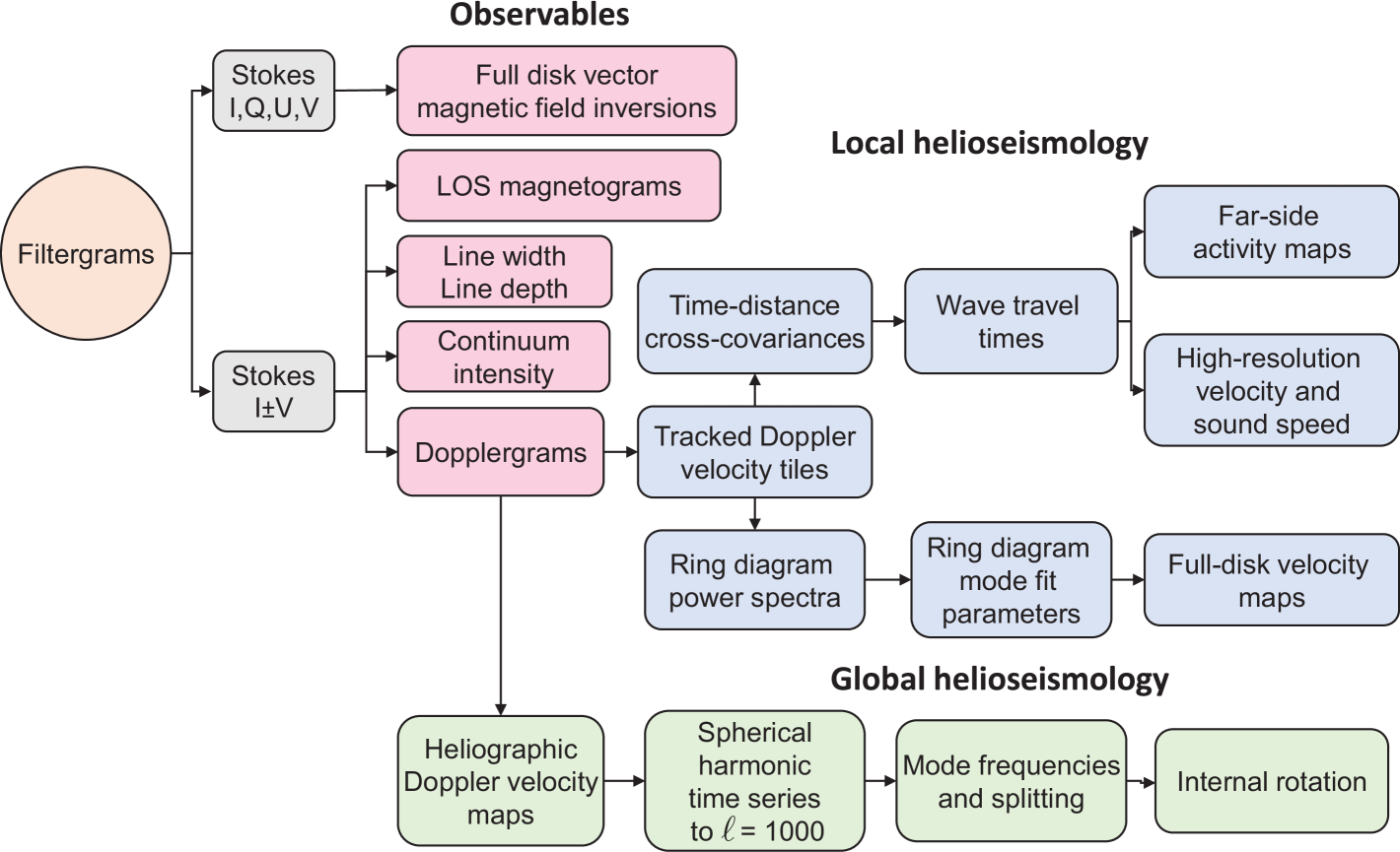
Figure 1 shows the simplified HMI data pipeline emphasizing data products related to helioseismology. Boxes on the right edge show final high-level data products. Users of HMI data can access any of the products via the SDO Joint Science Operations Center (JSOC)111jsoc.stanford.edu.
The Dopplergrams feed two helioseismology pipelines: global and local. The global pipeline remaps the full-disk Dopplergrams to heliographic coordinates, computes time series of spherical harmonics that reveal resonant acoustic-wave oscillations, determines mode frequencies and splittings, and performs inversions to determine internal rotation and sound speed profiles. Boxes in green near the bottom of the figure indicate the global-mode helioseismic data products. The HMI global pipeline analysis (Larson and Schou, 2018) is similar to that performed using data from the Michelson Doppler Imager (MDI: Scherrer et al., 1995; Kosovichev et al., 1997; Larson and Schou, 2015) on board the Solar and Heliospheric Observatory (SoHO: Domingo, Fleck, and Poland, 1995) in Solar Cycle 23. Others have extended the analysis to higher order modes (Reiter et al., 2015, 2020) and have applied alternative methods for inversion to determine rotation profiles (Korzennik and Eff-Darwich, 2024).
The local-helioseismology pipeline starts with tracked surface-velocity tiles that are then used in two analysis techniques: Ring Diagrams and Time-Distance. The blue boxes in the middle show local helioseismology products. The tiles in the synoptic pipeline are centered on a regular Carrington grid and tracked at a fixed rotation rate (Bogart et al., 2011a, b). Pipeline tiles have three sizes: , , and , and are spatially sampled at half the size of the tile out to from the disk center. The velocities are corrected for the motion of the spacecraft relative to that point on the Sun and for instrument sensitivity. Tiles are remapped from heliographic coordinates to Postel’s azimuthal equidistant projection. The data cubes formed by time series of tracked tiles form the basis for subsequent analysis.
The Ring-Diagram technique, initially suggested by Gough and Toomre (1983), was first developed by Hill (1988) to measure local flows at moderate depths beneath the solar surface, 15 - 30 Mm, depending on the tile size. Tiles for the HMI Rings synoptic pipeline (Bogart et al., 2011a, b) are tracked at the Carrington rate. The software performs a 3D Fourier spectral analysis of the cubes and fits the resulting shape and location of the rings of mode power at each frequency. The ring parameters are then inverted to resolve the depth dependence of the horizontal velocity. Additional details can be found in Section 3.1 and the HMI Rings Team website222hmi.stanford.edu/teams/rings/.
The Time-Distance helioseismology technique was pioneered by Duvall et al. (1993). Acoustic waves of a particular wavelength and frequency penetrate to a certain depth (wave turning point). By applying appropriate temporal and spatial filters, waves traveling in opposite directions between surface points can be identified, and the differences in travel times can be used to determine the velocity along the ray path. With assumptions about the ray propagation, an appropriate inversion for many points results in a map of subsurface motions (Kosovichev, 1996b). The method has been developed over the years and implemented in the HMI pipeline (see Zhao et al., 2012b for an introduction and a detailed description of the HMI analysis pipeline). The pipeline uses tiles tracked at the differential rotation rate to build up a map of flow vs depth for the near side of the Sun to a depth of Mm every 8 hours (see Section 3.2).
Lindsey and Braun (2000b) first realized that the largest spatial-scale waves could be used to detect perturbations on the far side of the Sun. Particular acoustic waves that originate at one point on the far side will follow well-defined paths whose reflection points can be detected in predictable patterns on the visible side of the Sun. By isolating specific combinations of such waves that originate at different locations on the far side, increasingly sophisticated maps of propagation delays can be constructed (Duvall and Kosovichev, 2001; Zhao, 2007; Zhao et al., 2019). Delays of a few seconds in the several-hour travel time of waves reveal locations on the far side where the magnetic field is strong (Chen et al., 2022).
Table 1 lists some of the most relevant helioseismology data series available in the HMI pipeline. The rest of this report discusses scientific results based on these data.
| JSOC Data Series | Method | Description |
|---|---|---|
| hmi.V_45s | Time series of full-disk Dopplergrams at 45 s cadence | |
| hmi.V_sht_gf_72d | Global | Spherical harmonic time series of HMI velocity data, gap-filled and detrended |
| hmi.V_sht_pow | Global | Power spectra of detrended and gap-filled time series |
| hmi.V_sht_modes | Global | Mode fits to the spherical harmonic power spectra, symmetric mode profile |
| hmi.V_sht_modes_asym | Global | Same as above but asymmetric profile |
| hmi.V_sht_2drls | Global | 2D RLS inversion for rotation profile from symmetric mode parameters |
| hmi.V_sht_2drls_asym | Global | Same as above using asymmetric mode parameters |
| hmi.rdVpspec_fd30 | Rings | Power spectra of tracked regions |
| hmi.rdVpspec_fd15 | Rings | Power spectra of tracked regions |
| hmi.rdVflows_fd30_frame | Rings | Inverted flows for tracked regions |
| hmi.rdVflows_fd15_frame | Rings | Inverted flows for regions |
| hmi.rdVfitsc_fd05 | Rings | Ring-diagram fits of flows and mode parameters for regions |
| hmi.tdVtimes_synopHC | Time-Distance | Travel times for 25 areas of |
| hmi.tdVinvrt_synopHC | Time-Distance | Subsurface flow fields |
| hmi.td_fsi_12h | Time-Distance | Time-distance far-side images |
| hmi.fsi_phase_lon_lat | Holography | Holography-method far-side images |
1.2 JSOC Data Access
The SDO Joint Science Operations Center (JSOC) Science Data Processing facility at Stanford receives SDO data in near-real time from the satellite downlink station. JSOC processes both HMI and Atmospheric Imaging Assembly (AIA: Lemen et al., 2012) data for use by the community. Quick-look data, such as magnetograms and solar far-side activity maps, are produced for space-weather studies. Definitive science data are generated with some delay, which can take several days, to ensure that all of the relevant calibrations that depend on time history are complete and that time series of sufficient duration are available.
Each data product is stored in a data_series that consists of a series of data records. The record is the basic unit of data and consists of keywords, segments, and links. Each data_series is organized around one or more prime keywords, such as time. Other keywords contain metadata describing the series or a particular record or segment. A segment is a collection of files with the actual data, typically one or more files in the FITS format. A link is a pointer to a segment in another data series associated with the same prime keywords.
For example, the HMI Dopplergrams are in the data series hmi.V_45s with records organized by the prime keywords t_rec and camera. Many other keywords provide information about the data in that record; for example, obs_vr provides the radial velocity of the SDO satellite relative to the disk center at the time of observation. This series has a single segment called Dopplergram, which is a FITS file with the 40964096 line-of-sight velocity image in m s-1.
By contrast, the ring diagram flow series, hmi.rdVflows_fd15_frame has prime keywords CarrRot and CMLon indicating the Carrington Rotation and central meridian longitude for a set of computed rings; there is one record for each of Carrington Longitude. For each record, there are two segments, Ux and Uy, that contain velocities in the zonal and meridional directions, respectively. In this series, each segment consists of 284 ASCII tables, one for each of the rings spaced every in longitude from E to W and in latitude between + and within of the disk center. For each ring pixel, the table provides the velocity computed at 31 target depths from 0.970 to 1.000 solar radii, along with uncertainties and other information.
The JSOC data series are managed by a Data Record Management System (DRMS). Various tools are available to query the database and export data. On export, the keywords, segments, and links are combined. A general introduction to SDO data access is available in the Guide to SDO Data Analysis333www.lmsal.com/sdodocs/doc/dcur/SDOD0060.zip/zip/entry/. For exploratory work, the web-based tool lookdata444jsoc.stanford.edu/ajax/lookdata.html is recommended. The export data tool provides various options for preprocessing and refining, extracting, or projecting data. The JSOC website555jsoc.stanford.edu/ provides more information. There are also Python tools for sunpy666docs.sunpy.org/en/stable/tutorial/acquiring_data/jsoc.html and solarsoft777www.lmsal.com/sdodocs/doc/dcur/SDOD0060.zip/zip/entry/sdoguidese6.html#x11-390006.3 tools for IDL.
2 Global Helioseismology Measurements
The primary goal of global helioseismology measurements is to provide estimates of resonant mode frequencies, amplitudes, line widths, and asymmetry, as well as parameters of the background convective noise. Mode frequencies are primarily used to determine the solar interior structure and differential rotation and their variations using helioseismic inversion procedures. In addition, the mode amplitudes, line widths, asymmetry, and background are valuable for studying the physics of solar oscillations and characterizing solar-cycle variations.
Continuous high-resolution HMI observations substantially extended the capabilities of global helioseismology measurements from the Global Oscillation Network Group (GONG) and Michelson Doppler Imager (MDI) and led to the development of new data analysis methods. Because of the telemetry restrictions for transmitting the observational data from SoHO, MDI’s full-disk -pixel Dopplergram images with a 1-min temporal cadence were transmitted only two months a year during the Dynamics campaigns. All other times the data were transmitted only after a ‘vector-weighted’ binning of the full-disk images, which reduced the spatial resolution by a factor of 4. These data were used to measure the frequencies of the oscillation modes in the range of the spherical harmonic degrees, , from 0 to 300 (aka the Medium- Program; Kosovichev et al., 1997). SDO orbit allows for the continuous and nearly uninterrupted transmission of HMI full-resolution -pixel Doppler images with a 45-sec cadence.
The HMI data analysis pipeline continues the MDI Medium- program. The data are processed by performing the spherical harmonic decomposition for the full-resolution -pixel Dopplergrams, and also by simulating the MDI vector-weighted binning to investigate potential systematic effects caused by the binning scheme. In addition, the frequency measurement procedure was substantially improved and thoroughly tested (Larson and Schou, 2018, 2024). These improvements made it possible to investigate potential systematic errors. In particular, it was determined that a signature of a high-latitude jet, which appeared in some inversions of the MDI data (Schou et al., 1998), was an artifact.
The global helioseismology analysis of the HMI data in the medium-degree range measures the mean frequencies of mode multiplets and the coefficients of a polynomial expansion to represent the mode frequency splitting as a function of azimuthal order, , using orthogonal polynomials (the so-called -coefficients). This frequency splitting results from the differential rotation and departures of the solar structure from spherical symmetry. The global helioseismology analysis also measures other properties of the oscillation modes, such as the mode amplitude, line width, and background noise level (Larson and Schou, 2015). Two models are used for fitting the oscillation line profiles, a symmetrical Lorentzian profile describing a damped harmonic oscillator and a non-symmetrical profile (based on the formulation of Nigam and Kosovichev, 1998), describing oscillations excited by acoustic sources localized in the subsurface layers. The mode fitting results and the inferred differential rotation profiles are available via the JSOC for these two models.
The precision of global helioseismology measurements is higher for longer observing periods. However, the analysis has to be performed for relatively short intervals to capture variations in the solar structure and rotation associated with solar magnetic activity. Hence the JSOC global heliosesimology pipeline fits time series that are 72-day and 360-day long. The oscillation power spectrum corresponding to a 72-day long time series is illustrated in Figure 2. This power spectrum is obtained by projecting the Doppler velocity images onto spherical harmonics, performing the Fourier transform for the spherical harmonic coefficients time series, and averaging the power over the mode multiplets after applying corrections for the rotational frequency splitting.
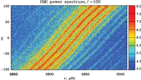
The power spectral density (on a logarithmic scale) as a function of frequency and the azimuthal order, , for a mode of the angular degree, , is shown in Figure 3. The change of slope in this diagram reflects the latitudinal changes in the solar rotation. The multiple lines (‘spatial leaks’) are caused by the leakage of the power of modes with the angular degrees in the vicinity of the target mode (mostly in the range of ) because the spherical harmonic transform is performed only in a visible hemisphere of the Sun. The mode leakage is calculated and taken into account in the data analysis (e.g. Korzennik et al., 2013).
The measurements (fitting the mode peaks in the power spectrum) are performed approximating the rotational splitting by polynomials of three orders, 6, 18, and 36, and available in the HMI data products hmi.V_sht_modes and hmi.V_sht_modes_asym (Table 1). The odd -coefficients in the 6-order approximation provide estimates of only the first three terms in the differential rotation, but the high-degree approximations resolve the evolving zonal flows (so-called ‘torsional oscillations’) and investigate their relationship to the solar activity. The 36-order approximation provides better latitudinal resolution than the 18-order approximation; however, the inversion results for the 36-order approximation may be noisier. Therefore, both approximations should be used for analysis. The even-degree -coefficients are used to study the aspherical structure of the Sun.
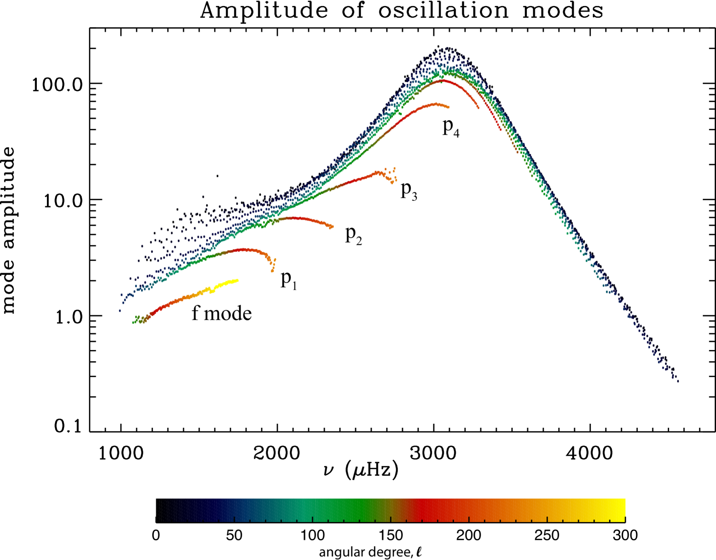

In addition, the data are analyzed at the Center for Astrophysics, Harvard & Smithsonian (CfA) for various time intervals using a novel technique (Korzennik, 2023). This technique uses optimal multi-taper power spectrum estimators to reduce the noise and fit the individual multiplets that are visible in the power spectrum (Korzennik, 2005). The rotational frequency coefficients are calculated from the individual frequencies for each multiplet. The frequencies and frequency splitting obtained by this technique from the HMI data are available at the CfA website888lweb.cfa.harvard.edu/˜sylvain/research/tables/ (Korzennik, 2023) and the JSOC data products su_sylvain.hmi_V_sht_modes_sym_v7 for fitting symmetric mode profiles and su_sylvain.hmi_V_sht_modes_asym_v7. for the asymmetrical profile. In particular, the HMI provides an opportunity to obtain high-precision measurements by using very long time series. Figures 4 and 5 show the amplitude and frequency measurements obtained from a 2304-day (6.3 years) long time series of observations of Doppler velocity. The mode amplitude is colored according to the mode angular degree. The amplitude of higher-degree modes is reduced because of stronger dissipation in the near-surface layers. The error bars in Figure 5 show the error estimates magnified by a factor of 2000. The work on identifying potential systematic uncertainties that may affect the inversion results for the solar rotation and structure is still actively pursued (Korzennik, 2023).
The oscillation modes of high angular degree () carry important information about the near-surface layers of the Sun. At high degrees, however, the spatial leaks get closer in frequency due to a smaller mode separation, and the peaks get wider and eventually overlap since the mode’s lifetime gets smaller. As a result, high-degree modes blend into broad ridges of power. Unfortunately, the properties of such ridges do not correspond to those of the underlying individual peaks. This is because the amplitudes of the spatial leaks are asymmetrical with respect to the targeted mode, and so the central frequency of the ridge is significantly shifted away from the underlying individual mode frequency. Therefore, fitting a ridge requires detailed knowledge of the distribution of power that leaks into the sidelobes adjacent to the targeted spectral peak.
Techniques for measuring properties of the high-degree modes have been developed (Korzennik et al., 2013; Reiter et al., 2020), but they have yet to be routinely applied for analyzing the HMI data. One approach consists of fitting the power ridges and correcting the resulting values by using a sophisticated model of the underlying power distribution of the modes that blend into such a ridge. The offsets between the underlying mode characteristics and the resulting modeled ridge properties are then used in a parametric formulation to derive underlying mode characteristics from measured ridge characteristics. The other approach consists of fitting a multimodal extended model to the observed ridge, which incorporates some a priori knowledge of the power distribution.
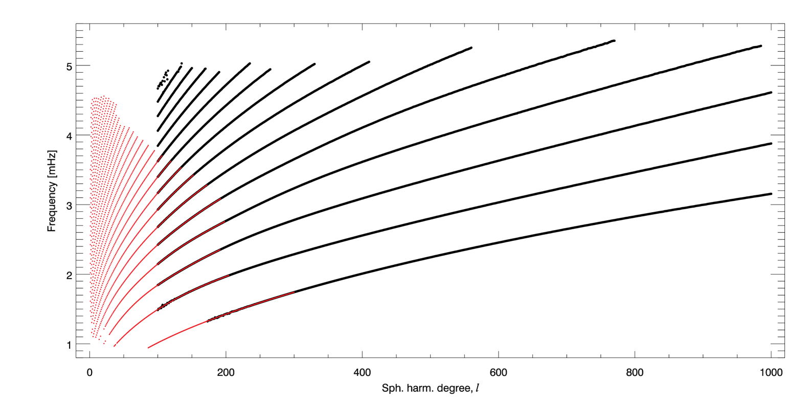
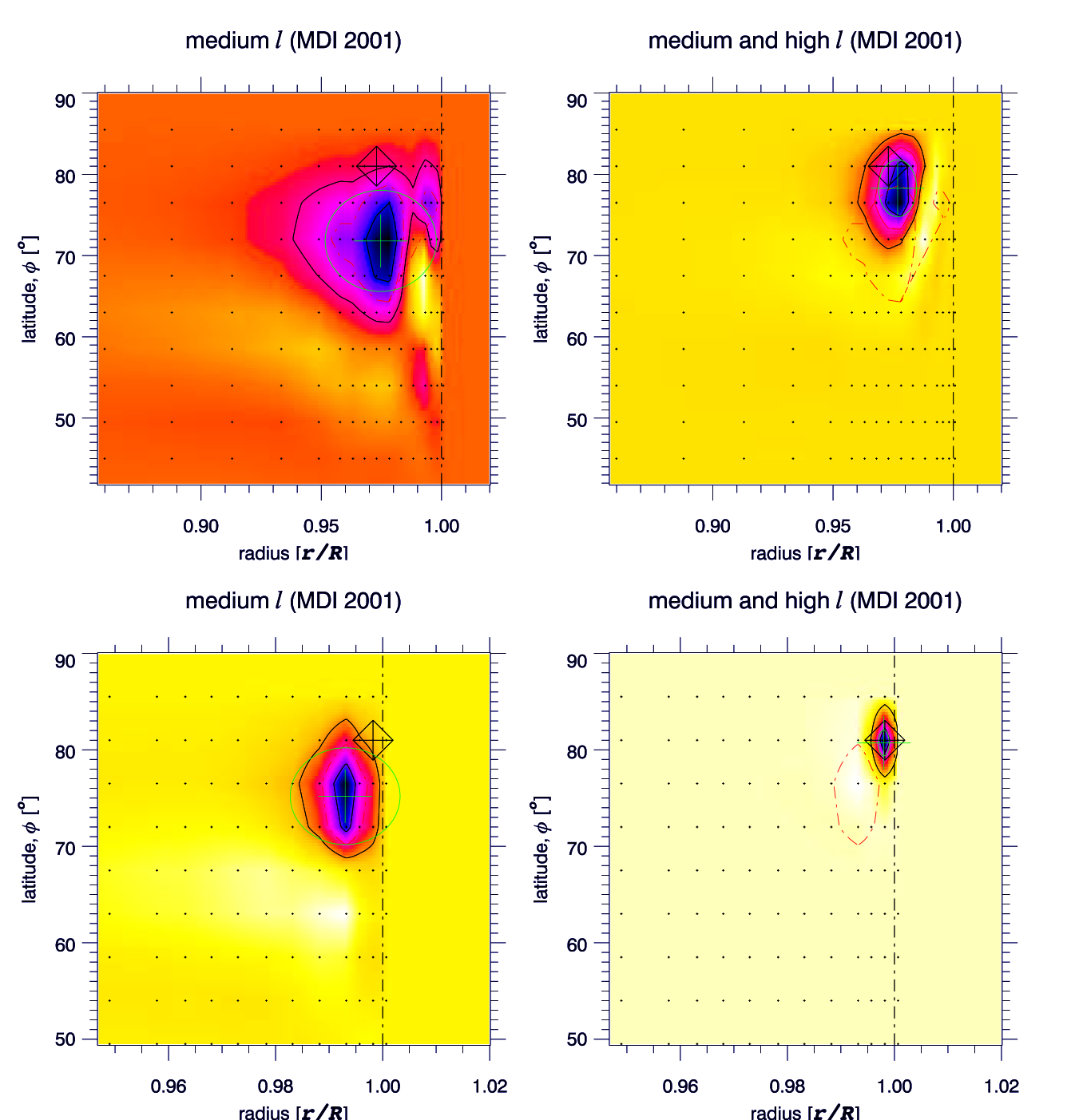
The extent and potential of these high-degree modes are illustrated in Figures 6 and 7, where we show the coverage in an diagram of the high-degree modes compared to the medium-degree ones, while Figure 7 compares the expected resolution, as indicated by averaging kernels, near the surface when including or not high degree modes in a rotation inversion. It has also been shown that the high-degree mode measurements can substantially improve the resolution of the solar structure in the near-surface shear layer (Reiter et al., 2015, 2020).
3 Local Helioseismology Techniques
Several techniques have been developed to measure and characterize large-scale mass flows on the Sun. Doppler imaging uses the Dopplergrams to measure the line-of-sight velocities of plasma motions on the solar surface. Correlation and Structure Tracking methods involve tracking the motion of magnetic features or intensity patterns over time. Local helioseismology methods enabled the inference of near-surface and deep subsurface flows from observations of solar oscillations. The Time–Distance method measures the travel times of acoustic waves between different points on the solar surface, while the Ring Diagram technique analyzes the power spectra of solar oscillations in localized regions; both methods determine flow velocities at various depths through which the observed waves propagate. The Helioseismic Holography method provides important information about acoustic sources of solar flares and quiet Sun regions and is routinely used for detecting and tracking sunspot regions on the far side of the Sun. In addition, new methods of Mode Coupling enabled the discovery and analysis of Rossby waves and inertial modes on the Sun.
3.1 Ring-Diagram Method
In the Ring-Diagram technique, small regions of the solar disk, typically with diameters of 5∘, 15∘, and 30∘, are tracked at the Carrington rotation rate for durations corresponding to their angular size (approximately 9.6, 28.8, and 57.6 hours, respectively). These regions are then remapped into solar latitude and longitude coordinates using the azimuthal equidistant (Postel’s) projection. A plane-wave approximation can be applied because the horizontal wavelengths of acoustic waves observed at these scales are significantly smaller than the solar radius. This enables us to calculate the power spectrum using three-dimensional Fourier transforms as a function of the horizontal wavenumber components, and (corresponding to longitude and latitude directions), and temporal frequency. The resulting spectrum exhibits a characteristic structure resembling nested “trumpets” along the frequency axis. When examining horizontal slices of this power distribution at constant frequencies, distinct rings for each radial order are observed (Figure 8).
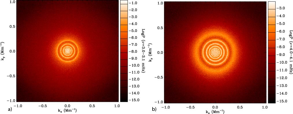
This distinctive pattern gives rise to the term “ring diagram analysis” for this technique. The presence of a velocity field, , introduces perturbations to the wave frequency producing an apparent frequency shift, which can be expressed as: , where and represent the components of the velocity vector along the longitude () and latitude () directions.

The 3D power spectrum is analyzed using two fitting methods to estimate the horizontal velocity field. In the first approach (Basu and Antia, 1999), implemented in the HMI pipeline as hmi.rdVfitsc data series (Table 1, HMI Observables), the spectrum is fitted at a set of selected frequencies (Figure 9).
The second method, developed by Schou and Bogart (1998), involves unwrapping the 3D power spectrum. For each wavenumber (where ), a cylindrical section is extracted by interpolating the original three-dimensional spectrum onto a uniform grid in azimuth angle at each frequency. This spectrum is then Fourier filtered in and subsampled to reduce computational time. While this approach is significantly faster than the first method, it results in a smaller number of measurements. The velocity field is fitted for each , and in the HMI pipeline, the resulting fitted parameters are provided in the hmi.rdVfitsf data series. It’s worth noting that this second method is also employed in the GONG pipeline (Corbard et al., 2003).

In ring-diagram analysis, we infer the horizontal velocity variation with depth using the relation , derived from spherical harmonics, to estimate an effective angular degree, . These estimated values are then interpolated to the nearest integral value. Subsequently, we apply inversion methods from global helioseismology to analyze the data. The ring-diagram fitted parameters, and , plotted as a function of and the radius of the mode inner turning points, , in Figure 10, illustrate the depth coverage of the ring-diagram method. The inner turning point defines the deepest point of wave propagation into the Sun’s interior from the surface. It depends on the ratio of the mode angular degree, , and frequency .
The HMI pipeline employs the Optimally Localized Average (OLA) technique, as described by Backus and Gilbert (1968) and further elaborated by Basu and Antia (1999). Another inversion method commonly used is the regularized least squares (RLS). In the HMI pipeline, the OLA method is used to calculate the inverted flows, which are provided in the data series hmi.rdVflows_fd15_frame and hmi.rdVflows_fd30_frame (Table 1 in Section 1: HMI Observables). These calculations are performed by the rdvinv module (Bogart et al., 2011a).

The maximum depth achievable in this analysis is approximately equal to the size of the tile under examination. For instance, when analyzing a 15-degree (30-degree) region, we can infer flows from very close to the surface down to depths of about 15 Mm (30 Mm). It’s important to note that as fewer waves penetrate deeper layers, the uncertainty in the horizontal location increases with depth (Figure 11).
The analysis of smaller tiles presents additional challenges due to the reduced number of measurements. This limitation makes the inversion process more difficult. As a result, the HMI pipeline currently does not provide inversion results for 5-degree tiles (Bogart et al., 2023).
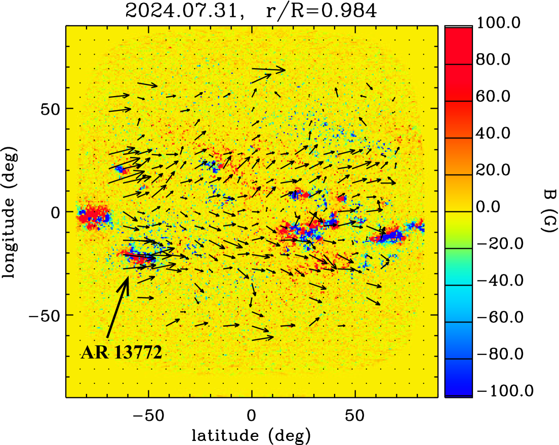
A useful data product for ring-diagram analysis is the Magnetic Activity Index (MAI), which quantifies the level of magnetic activity in each analyzed region. The MAI is calculated by the HMI processing pipeline. Using the same mappings and temporal and spatial apodizations as the tracked regions, the absolute values of all pixels in corresponding HMI line-of-sight magnetograms with an absolute value greater than 50 G ( 50 G) are averaged. The magnetograms are sampled once every 48 minutes for this calculation, as described by Bogart et al. (2011a, b). Arrows in Figure 12 illustrate a typical horizontal flow map at a depth of about 11 Mm plotted over the corresponding surface magnetogram. Results of the ring-diagram method are discussed in Sections 5, 9, 9.2.3, and 9.2.1.
3.2 Time-Distance Method
Acoustic waves are believed to travel between the Sun’s surface locations through the solar interior along curved paths. The acoustic travel times from one surface location to the other can be measured, as a function of the distance between the two locations, by time-distance helioseismology (Duvall et al., 1993) by cross-correlating two time-sequences of oscillations observed at those surface locations. One travel time can be measured from both the positive lag and the negative lag of the cross-correlation function, corresponding to the waves traveling from one location to the other and traveling in the opposite direction, respectively.
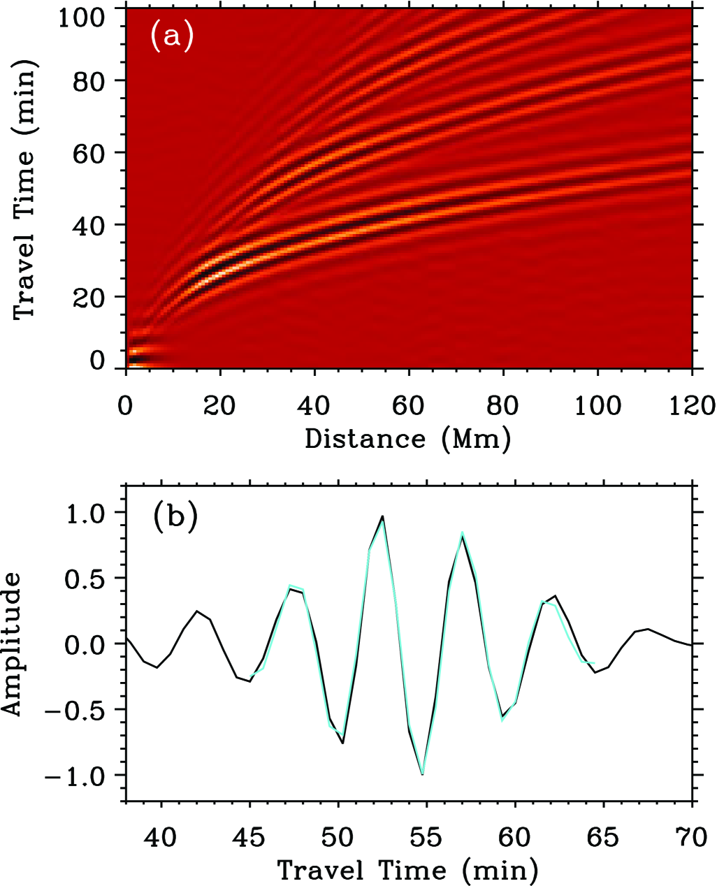
A combination of the cross-covariance functions calculated for different distances and lag times forms a time-distance diagram (Figure 13a). It shows ridges corresponding to wave packets arriving at a particular distance after multiple reflections. The lowest ridge represents direct waves (called the first skip). Figure 13b illustrates a cross-covariance function of the first skip (black) for a distance of 109 Mm and a Gabor-wavelet fitting function (green) that measures a phase travel time of 52.28 min.
Small perturbations in the acoustic wave travel times reflect changes in the physical conditions of the solar interior along the wave paths. For instance, a plasma flow along the wave’s propagation direction will shorten the travel time, while a flow in the opposite direction will lengthen it. Thus, the travel-time shifts between waves traveling in opposite directions along the same path serve as indicators of interior flows and can be measured from observation. Thus, the mean of these travel time shits is related to the sound-speed variations, and the difference between the shifts is caused by subsurface flows.
A time-distance helioseismic analysis pipeline was developed using the HMI Doppler-velocity data (Zhao et al., 2012b; Couvidat et al., 2012). The primary data product from this pipeline is subsurface flow fields of 25 patches of heliographic degrees, covering the near-full-disk area of , with a spatial sampling rate of pixel-1 and a depth coverage from the surface up to around 20 Mm. In this analysis, each patch is tracked and remapped using Postel’s projection.
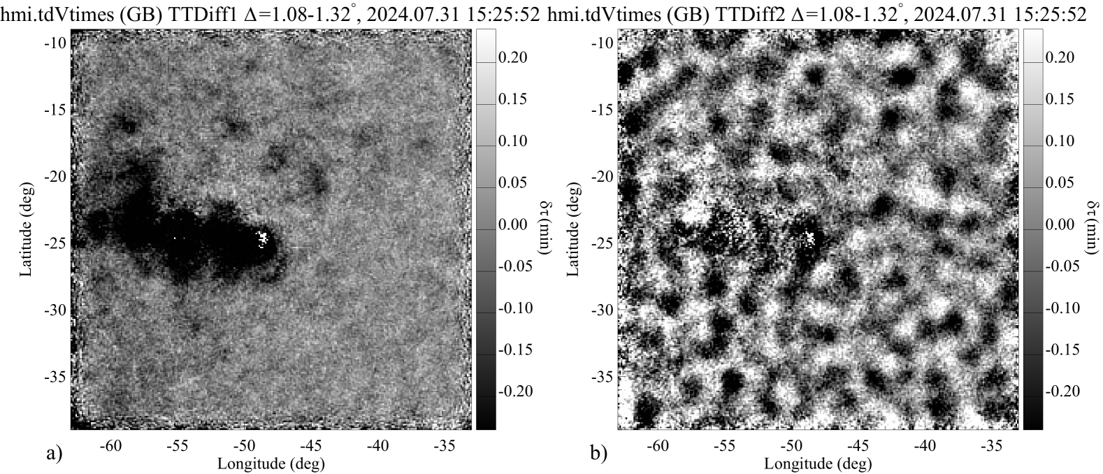
The pipeline employs two methods to fit for the travel times, Gabor wavelet fitting (Kosovichev and Duvall, 1997) and linear fitting (Gizon and Birch, 2002). The HMI data product hmi.tdVtimes_synopHC contains fitted travel times, with data segments ‘Gabor’ from the Gabor wavelet fitting and ‘GB’ from the travel times defined by Gizon and Birch (2002). The travel times are calculated for 11 travel distance ranges (Table 1 in Zhao et al., 2012b), which correspond to the range of depths of acoustic wave turning points from 0 to Mm. Figure 14 illustrates (a) the mean travel times (defined as TTDiff1 in data product hmi.tdVtimes_synopHC), which are sensitive to the sound-speed variations, and (b) the travel time difference (TTDiff2), which is mostly sensitive to the vertical flow velocity and flow divergence. The travel times are calculated for a patch centered at latitude and longitude, and for an 8-hour time interval centered at 15:32:52 UT on 2024.07.31. This is the same date as in Figure 12 illustrating the flow map from the ring-diagram pipeline. The interval of the travel distances, heliographic degrees, covers a depth range of up to 5.1 Mm. In panel (a), the negative travel time variations of TTDiff1 (dark areas) reveal the travel time reductions beneath active region AR 13772 (indicated in Figure 12). In panel (b), the negative travel-time patches are caused by the diverging supergranulation flows.
With theoretically derived sensitivity kernels (e.g., Birch and Kosovichev, 2000; Böning et al., 2016; Hartlep and Zhao, 2021), which relate the subsurface properties to the surface measurements using a solar model, one can set up linearized equations and solve them for the solar interior flows and sound-speed variations using inversion techniques (e.g. Kosovichev, 1996b; Jensen, Jacobsen, and Christensen–Dalsgaard, 1998; Couvidat et al., 2005).
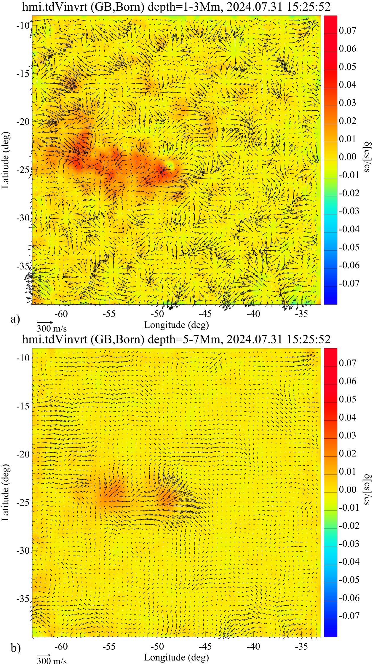
Two sets of sensitivity kernels, ray-approximation kernels (Kosovichev and Duvall, 1997) and Born-approximation kernels (Birch, Kosovichev, and Duvall, 2004; Birch and Gizon, 2007), are used in the inversion codes. The data product hmi.tdVinvrt_synopHC contains inversion results, with ‘vx’ for subsurface east-west direction velocity, ‘vy’ for subsurface north-south direction velocity, ‘vz’ for vertical velocity, and ‘cs’ for subsurface wave-speed perturbations. Keywords ‘Gabor’ and ‘GizonBirch’ define which fitted travel times are used, and ‘Born’ and ‘Raypath’ define which sensitivity kernels are used (see HMI Time-Distance Products website999jsoc.stanford.edu/HMI/TimeDistance.html). Figure 15 illustrates the subsurface sound-speed variations and the horizontal flows at two depth ranges, 1 – 3 Mm and 5 – 7 Mm. In the shallower layer, the flow pattern is dominated by supergranulation, while in the deeper layer, the supergranulation flows diminish, and the flow map reveals East-West flows associated with the active region. Both cases show enhancements in the sound speed beneath the active region.
The flow fields become available every 8 hours, several days after the observing date. From these subsurface flow maps, one can compute the divergence and horizontal vorticity at various depths, which then can be used to study, e.g., properties of supergranules (DeGrave and Jackiewicz, 2015). These maps can be used to study the long-term evolution of near-surface zonal and meridional flows (Zhao, Kosovichev, and Bogart, 2014; Getling, Kosovichev, and Zhao, 2021; Mahajan, Sun, and Zhao, 2023).
Time-distance helioseismology is used not only to infer local subsurface flow fields but also to study global flows. Inference of the Sun’s deeper meridional circulation has been studied by various authors in the past decade using HMI observations (see Section 7). Time-distance helioseismology has also been developed to map active regions on the far side of the Sun (see Section 11). The Time-Distance Helioseismology101010jsoc.stanford.edu/data/timed/ website provides the far-side images and also full-disk merged subsurface flow maps obtained using the Gabor wavelet travel-time fitting and the Raypath sensitivity kernels.
3.3 Mode Coupling
Normal-mode coupling, a seismic technique with a long history in geophysics (see, e.g. Dahlen and Tromp, 1998), has seen limited use in helioseismology. This method is similar to global helioseismology, but instead of interpreting eigenfrequencies, it is focused on analyzing the mode eigenfunctions. Non-spherically symmetric flows and structure variations in the Sun perturb the eigenfunctions calculated for a reference solar model. These perturbations can be considered in terms of coupling of the theoretical eigenfunctions. Therefore, this technique is called the Mode Coupling. Unlike eigenfrequencies, which are scalar quantities, eigenfunctions are vectors and require a different measurement technique to analyze observed data.
The key measurement involves analyzing cross-correlated Fourier components of the Sun’s wavefield across different frequencies and spatial scales. This approach is somewhat analogous to estimating the power spectrum of solar acoustic waves. However, instead of focusing on the power spectrum of individual modes, the method considers the cross-spectra of distinct acoustic modes characterized by the radial order , angular degree and order and frequency with the modes with different and frequency . In the absence of non-spherically symmetric perturbations, the stochastic excitation of acoustic waves would yield zero correlation. However, the presence of flows and perturbations in the Sun with specific spatial and temporal scales result in enhanced power in the cross-correlation measurements interpreted as the mode coupling. The analysis of the enhanced power at certain scales reveals perturbations in the Sun’s structure. Woodard (1989) was the first to describe how the Sun’s differential rotation across latitudes distorts its oscillation modes. Since then, this method has been applied to various topics such as meridional circulation and convection (e.g. Lavely and Ritzwoller, 1992; Roth and Stix, 2008; Schad, Timmer, and Roth, 2013; Woodard, 2016; Hanasoge, 2017, 2018). The method of mode-coupling has been successfully used to detect various types of inertial waves in the Sun, including Equatorial Rossby waves (Mandal and Hanasoge, 2020; Mandal, Hanasoge, and Gizon, 2021), high-latitude inertial waves (Mandal and Hanasoge, 2024), and high-frequency retrograde modes (Hanson, Hanasoge, and Sreenivasan, 2022).
4 Solar Structure
Helioseismology has provided detailed inferences of the solar internal structure by applying sophisticated techniques for the so-called inversion of the data (Kosovichev, 2011a; Basu, 2016). This has led to strong constraints on our understanding of solar evolution (Christensen-Dalsgaard, 2021).
Early helioseismology data allowed us to determine the structure of the Sun by inverting the available frequencies (e.g. Gough et al., 1996). The inversions showed that the structure of standard solar models is in very good agreement with the structure of the Sun; the relative sound-speed differences are less than 0.5%, while relative density differences are a few percent. These results have not been changed by the HMI data, as can be seen in Figure 16.
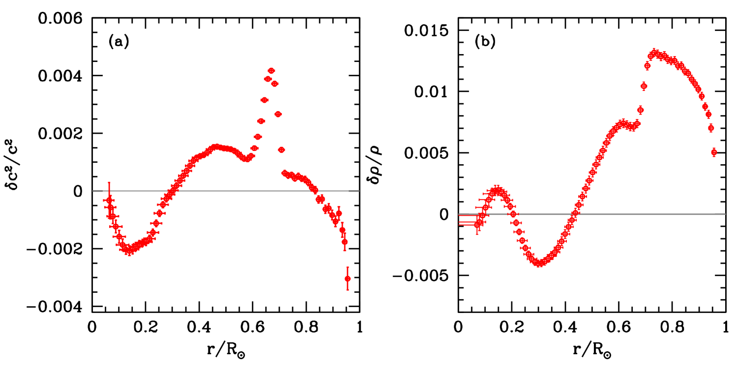
Early inversions, including the one shown in Figure 16 were usually done with p-modes that ranged in spherical harmonic degree from to or 250, and hence, the results are not reliable for radii larger than about 0.98 R⊙. The high spatial resolution data of HMI have allowed the frequencies of higher modes to be determined, and these inversions show that closer to the surface, the sound speed of our models is significantly higher than that of the Sun, with sound-speed differences exceeding 1% (Reiter et al., 2015, 2020).
4.1 The Issue of Solar Abundances
Perhaps the most pressing uncertainty when it comes to solar structure is that the solar heavy element abundance is in dispute. Model S, a standard solar model that showed that the structure of the Sun quite well (Gough et al., 1996), was constructed with (henceforth GN93: Grevesse and Noels, 1993). Within a few years, updated analyses decreased the estimated solar metallicity to (henceforth GS98: Grevesse and Sauval, 1998). This decrease in metallicity worsened the match between solar models and the Sun — the decrease in metallicity decreased opacities, which in turn made the convection zone shallower. This, however, is not the end of the story. Using 3D model atmospheres and non-LTE calculations for abundances, Asplund, Grevesse, and Sauval (2005) claimed that the solar metallicity is even lower, . This group recently revised the abundances upward to (Asplund, Amarsi, and Grevesse, 2021). Earlier, an independent group of Caffau et al. (2010), using a different 3D model atmosphere and non-LTE effects, obtained a higher metallicity, , similar to that of GS98. More recently, Magg et al. (2022) derived an even higher metallicity of . The potential systematic uncertainties in these measurements and the directions for further studies were discussed by Lind and Amarsi (2024).
The issue with the uncertainty in the solar chemical composition is that it makes the structure of standard solar models uncertain. Low metallicities imply lower opacities, which in turn makes the convection zone more shallow; this introduces large differences between the sound speed and density profiles of low-metallicity models and the Sun. Among other issues is the fact that the convection-zone helium abundance of low-metallicity models is lower than the helioseismically determined one. The small frequency separations of low-metallicity models do not match observations either (Basu and Antia, 2008, and references therein). However, all these issues are ultimately connected to the lowered opacity. If opacities are higher than the calculated opacities, and experimental results suggest that iron opacities are higher than calculated (Bailey et al., 2015), then these discrepancies can go away. However, the experimental results are not easy to interpret, and additional experiments to determine chromium and nickel opacities (Nagayama et al., 2019) have yielded results that were not expected. Thus, the experimental issue of opacities remains unresolved. On the other hand, we note that opacity investigations can be guided by inferences of opacity from helioseismic inversion (e.g. Buldgen et al., 2025).
The flux of CNO neutrinos gives an independent measure of abundances, and results from the BOREXINO collaboration (Borexino Collaboration et al., 2020) reject the low-metallicity models at about a level. The neutrino results, however, are sensitive to the metallicity of the solar core, and consequently, there have been suggestions that the Sun may have a low-metallicity convection zone but a higher-metallicity core as a result of planet formation (Kunitomo, Guillot, and Buldgen, 2022). While most helioseismic results appear to support the high-metallicity solution, there are some inversion results, (e.g. Buldgen et al., 2017, 2024a) that find a low-metallicity solution in the convection zone. Note that these inversions explicitly use the equation of state, which may be uncertain, and also lack precision. However, it is clear that even high metallicity models do not match the Sun perfectly, and much more work needs to be done to understand the physical process inside the Sun (Buldgen et al., 2024b).
4.2 Seismic Solar Radius
The MDI and HMI data provided the capability to observe with unprecedented accuracy the surface gravity oscillation (f) modes, the frequency of which is not sensitive to sound-speed variations that can be caused by the surface magnetic activity. These data have been used to infer the seismic radius of Sun (Schou et al., 1997) and its variations with solar cycle (Antia et al., 2000; Dziembowski, Goode, and Schou, 2001; Kosovichev and Rozelot, 2018).
The f-mode frequencies are sensitive to the sharp density gradient in the near-surface layers, occupying about the top 5% of the solar radius. The low-frequency medium degree f-modes in the range of = 137,- 300 observed by the HMI concentrate the kinetic energy within a layer of approximately 15 Mm, or about 2% of the whole solar radius. That means that these f-mode radii are well below the subphotospheric superadiabatic boundary layer, which is located about 0.08 Mm below the photospheric surface. The comparison of the observed f-mode frequencies with those calculated for standard solar models provided an accurate estimate of the solar radius used as a reference in astronomy. So far, the resulting scaled f-mode radius values are lower than the photospheric radius deduced from optical observations by about 310 km (Schou et al., 1997) and 203 km (Antia, 1998). This discrepancy was explained as a difference of 333 8 km between the height at the disk center where the optical depth at = 1, and the inflection point of the intensity profile on the limb (Haberreiter, Schmutz, and Kosovichev, 2008). They concluded that the standard radius must be lowered by this quantity to be 695.66 Mm, close to the value adopted by IAU in 2015.
Takata and Gough (2024) have proposed inverting the p-modes, which react differently from the f-modes. They assert that the method is more robust albeit more-or-less, consistent with what is suggested by the f-mode analyses, estimating the solar photospheric radius to be 695.78 0.16 Mm. This accounts for a difference of 210 km compared with the reference model of = 695.99 Mm used by the authors.
The analysis of the low-frequency medium-degree f-modes in the range of = 137 – 299, the data covering nearly two solar cycles, from April 30, 1996, to June 4, 2017, showed that the mean seismic radius was reduced by 1 – 2 km during the solar maxima and that most significant variations of the solar radius occur beneath the visible surface of the Sun at a depth of about Mm, where the radius is reduced by 5 – 8 km. These variations can be interpreted as changes in the solar subsurface structure caused by the predominately radial kG magnetic field (Kosovichev and Rozelot, 2018).
4.3 Solar Asphericity
4.3.1 Asphericity of the solar surface
Most inversions have been done assuming that the structure of the Sun follows spherical symmetry. There have been few studies of the asphericity in structure, mainly because the signal of asphericity, which lies in the even-order splitting coefficients, is very small. Most previous results (e.g., Kuhn, 1988; Antia et al., 2001; Antia, Chitre, and Thompson, 2003) seem to imply that there are small deviations from sphericity close to the surface. It is possible to extract information concerning the coefficients of rotational frequency splitting, , discussed in Section 2. The odd coefficients ( = 1, 3 …), , , , …, measure the latitudinal differential rotation, whilst the even coefficients , , , …, are a sensitive probe of the symmetrical (about the equator) part of the distortion described by Legendre polynomials .
According to von Zeipel (1924) theorem, solar limb contours of temperature, density, or pressure should be nearly coincident near the photosphere. Rotation, magnetic fields, and turbulent pressure are the largest local acceleration sources that violate the von Zeipel theorem (Dicke, 1970). Since (geometrical) asphericities are relatively small in the Sun, we may describe the distance from the center (for instance, for a level of isodensity , but the same would happen to a level of isotemperature or isogravity) by:
| (1) |
where is the mean limb contour radius, the angle to the symmetry axis (colatitude) and is the Legendre polynomial of degree . The asphericity shape coefficients, , are called quadrupole for = 2 () and hexadecapole for (). Terms of higher orders are conventionally named by adding ‘pole’ to the degree numeral prefix. It is straightforward to determine the oblateness parameter (the relative difference between the equatorial and polar radii), , from Equation 1 in terms of the asphericity coefficients, , , and , using the standard definition of Legendre polynomials, as ; higher-order splitting coefficients are too uncertain to be useful.
The measured splitting coefficients are related to the shape coefficients through a normalization factor . An efficient method for calculating this factor was developed by Kuhn (1988), who showed that it was possible to invert the splitting data to obtain the structural asphericity using the relation: . Assuming = , as this analysis is conducted only very close to the surface (i.e., the seismic radius at the surface), the corresponding scaling factors are:
where the are measured in Hz.
It was shown that the asphericity of the Sun changes from the solar minimum to the maximum. During the solar minimum (from 1996 to 1998) the asphericity was dominated by the and terms, the contribution being negligible. At the time of high activity, all these components have a significant effect. The asphericity of the Sun is strongly affected during the solar cycle progression (Rozelot, Kosovichev, and Kilcik, 2020).
4.3.2 Asphericity of the convection-zone base
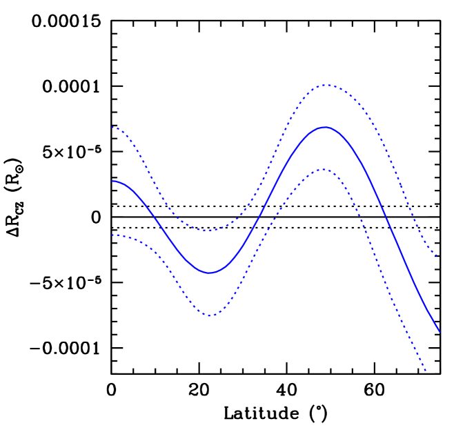
Many early attempts to determine the asphericity in the solar structure had been focused on determining whether or not the base of the convection zone has any asphericity. The base of the convection zone (CZ) is where the tachocline is located. The tachocline is the thin shear layer that separates the differentially rotating convection zone from the uniformly rotating interior (see Section 6). The tachocline is known to be prolate in shape (Gough and Kosovichev, 1995; Antia, Basu, and Chitre, 1998; Charbonneau et al., 1999), raising the question of whether the base of the convection zone is spherically symmetric. It was argued that the tachocline could drive meridional flows (Zahn, 1992) and that these flows must affect the thermal balance of the layers and could influence where the layer becomes unstable to convection, thereby causing the base of the CZ to deviate from spherical symmetry (Gough and Kosovichev, 1995). These authors claimed a difference of no more than between the convection zone base at the pole and the equator, while others derived an upper limit of on the asphericity of the CZ base (Basu and Antia, 2001). A more recent attempt at determining the asphericity that used HMI data (Basu and Korzennik, 2024) gives an upper limit of R⊙ departure from the spherically symmetric position of the base of the convection zone. Analysis of the – splitting coefficients indicates that deviation from sphericity is more complicated than a simple prolate or oblate spheroid, as can be seen from Figure 17. If one assumes that the cause of the asphericity is the effects of magnetic fields on solar structure then the shift in the base of the convection zone implies a strong hypothetical magnetic field of about kG. This is consistent with earlier upper limits on the magnetic field at the base of the convection zone (e.g. D’Silva and Choudhuri, 1993; Basu, 1997; Antia, Chitre, and Thompson, 2003).
4.4 The Sun as a Physics Laboratory
The high precision of the helioseismic inferences makes them sensitive to even quite subtle effects in the physics of the solar interior, allowing sensitive tests of the physics used in solar-model computations.
The first full inference of the solar internal sound speed (Christensen-Dalsgaard et al., 1985) indicated a need to increase the opacity in the radiative interior compared with the then current opacity tables, as later confirmed by new opacity calculations (e.g. Rogers and Iglesias, 1992). Helioseismic inferences of opacity were further explored by Gough and Scherrer (2002) and Buldgen et al. (2025), in the latter case also related to the issues caused by the revisions in the solar abundances (see also Section 4.1).
The solar sound speed depends sensitively on the thermodynamic properties of the solar plasma, including the adiabatic compressibility . From the helioseismic inference of , Elliott and Kosovichev (1998) inferred that the then-current advanced tables of thermodynamic properties had ignored significant relativistic effects on the electrons at the conditions of the solar core. This is corrected in the tables now used; however, the example illustrates the sensitivity of helioseismology to detailed aspects of solar interior physics. Basu, Däppen, and Nayfonov (1999) made a comparison of the inferred in the solar convection zone with two independent sets of thermodynamic tables, finding significant but different discrepancies between the Sun and the models in both cases. Such investigations have the potential to further improve our understanding of the thermodynamic properties of plasmas under extreme conditions; they would be greatly assisted by the availability of reliable helioseismic data for modes of higher degree than currently available (Di Mauro et al., 2002). A closely related issue is the helioseismic determination of the solar envelope helium abundance (Kosovichev, 1993; Basu and Antia, 1995).
Bellinger and Christensen-Dalsgaard (2022) considered the constraints on nuclear-reaction parameters provided by solar observations. They found that helioseismic data provided a strong constraint, greatly improving the theoretical or experimental uncertainty on the basic and the reaction rates, while the neutrino observations, in particular, constrained the reaction rate.
Moving beyond standard solar models, helioseismology has also been used to constrain more exotic physics. An important issue is the nature of the dark matter that seems to dominate the dynamics of galaxies. One candidate is the so-called weakly interacting massive particles (WIMPS). If present in the solar interior, even in small numbers, their expected long mean free paths could provide an efficient source of energy transport, hence cooling the solar core. In the early days of helioseismology and solar neutrino studies, this was seen as a way to account for the apparently low flux of solar neutrinos (e.g. Faulkner and Gilliland, 1985; Spergel and Press, 1985). Although the apparent solar neutrino deficit has now been identified as caused by neutrino flavor transitions, the Sun still provides constraints on the properties of potential dark-matter particles (e.g. Lopes, Kadota, and Silk, 2014; Vinyoles et al., 2015).
Structure inversion results are also being used for more speculative studies. For instance, Bellinger et al. (2023) examined what would happen if there were a black hole in the core of the Sun. They find that models of the Sun born around a black hole whose mass has since grown to approximately are compatible with current helioseismic results. In other investigations, Hamerly and Kosovichev (2012) and Bellinger et al. (submitted) examined what would happen if the Sun had a dark matter core. Interestingly, they find that the sound-speed profile of a solar model with a dark core appears to have a better agreement with the Sun than standard models. However, this improved agreement is by no means evidence of dark matter since a metal-rich core would give a similar result; more precise measurements of frequencies of low-degree p-modes and g-mode observations may constrain a dark-matter core inside the Sun.
It should be kept in mind that the use of helioseismology to constrain the physics of the solar interior depends critically on constraining other uncertainties in solar modeling than the one under study. Even so, it is clear that the Sun offers valuable information on matter under extreme conditions, supporting basic physics and its use in modeling other stars.
5 Convection and Large-Scale Flows
5.1 Brief Introduction
Thermal convection is the primary mechanism for energy transport in the Sun’s outer envelope, which encompasses roughly one-third of its radius. This process is responsible for energy transport and drives the complex fluid motions and magnetic fields observed at the solar surface. Deciphering the intricate dynamics within the Sun is crucial for our understanding of many solar phenomena, including the solar cycle, the formation and evolution of active regions, and their influence on space weather.
Previous studies revealed three primary components of solar convection: granulation, supergranulation, and giant cells (e.g., Nordlund, Stein, and Asplund, 2009). While the structure and dynamics of granulation are studied in detail using high-resolution observations of the solar surface and numerical simulations, the origin of supergranulation is still a puzzle (Rieutord and Rincon, 2010), and the existence of the giant cells is a subject of debate.
The initial studies of supergranulation by time-distance helioseismology using the MDI data revealed that the horizontal outflows that are observed on the surface by tracking the motion of granules or observing the Doppler shift extend several Mm below the surface (Duvall et al., 1997; Kosovichev and Duvall, 1997). Evidence of converging flows was at a depth of about 10 Mm, which gave an estimate of the average depth of supergranules of Mm (Zhao and Kosovichev, 2003). The typical horizontal velocity of the supergranular flows is about 300-500 m s-1. However, the vertical velocity is substantially lower, about 10 m s-1, which is rather difficult to measure. To overcome this difficulty, Duvall and Birch (2010) suggested averaging the signals from a large set of supergranules and found 10 m s-1 upflows at the center and downflows of about 5 m s-1 at the boundaries of such ‘averaged supergranule.’
In addition, studies of the supergranulation dynamics deduced from time-distance helioseismology of surface gravity waves (f-mode) revealed vorticity caused by the Coriolis force and a wave-like motion of the supergranulation pattern. The latter result added a new element to the long-standing puzzle of the super-rotation of supergranulation (Duvall, 1980; Meunier and Roudier, 2007). This phenomenon could be explained by the interaction of convection modes with the near-surface rotational shear layer (Green and Kosovichev, 2006). However, the calculated phase speed was lower than the observed super-rotation; therefore, some other effects must be involved, such as subsurface magnetic field (Green and Kosovichev, 2007) or non-linear dynamics (Rincon and Rieutord, 2018). The photospheric convection spectrum constructed from the MDI observations showed distinct peaks representing granules and supergranules but no features at wavenumbers representative of mesogranules or giant cells (Hathaway et al., 2000).
The uninterrupted high-resolution full-disk observations provided by HMI have significantly enhanced our ability to investigate these internal processes, particularly in the areas of convection and large-scale flows. This section reviews key findings from HMI observations, discusses the methods used to measure solar flows, and examines the challenges in modeling and interpreting these phenomena.
5.2 Structure and Dynamics of Supergranulation
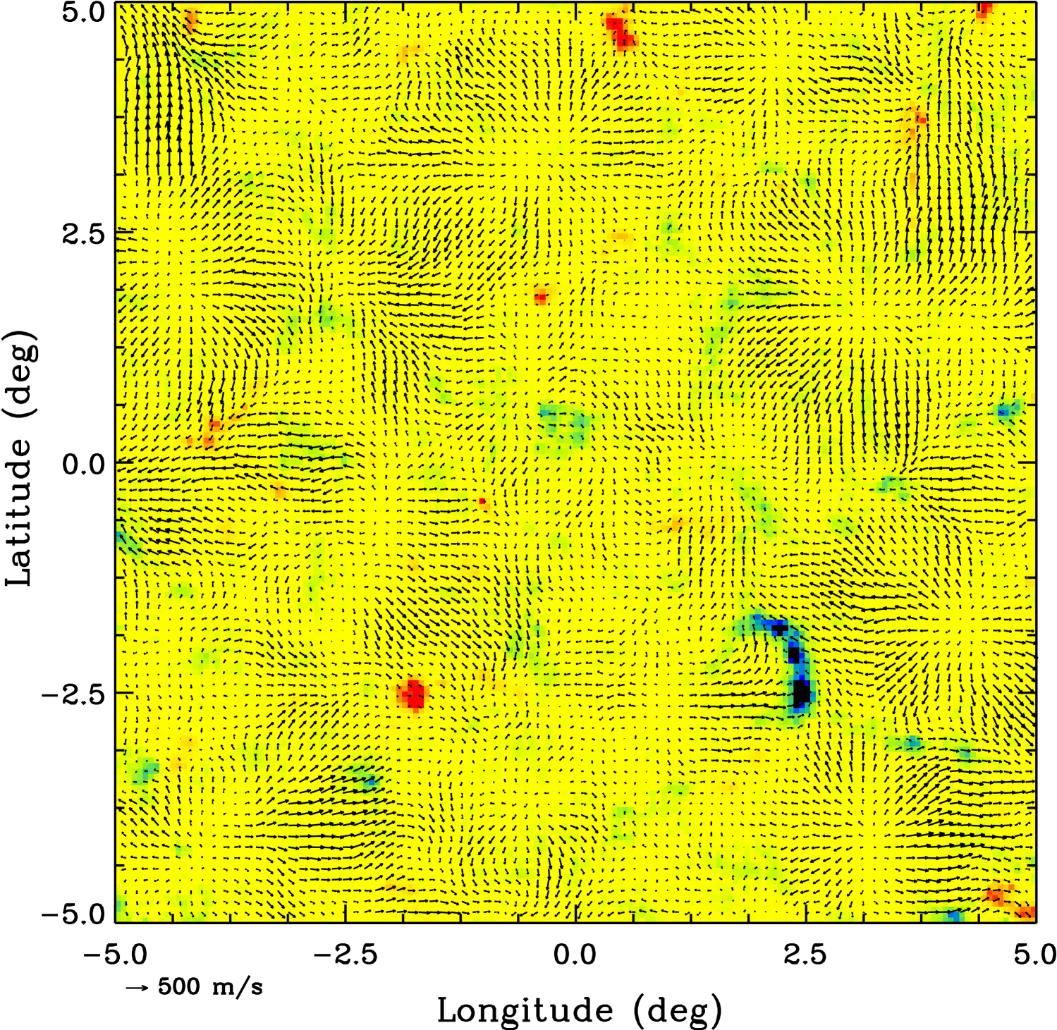
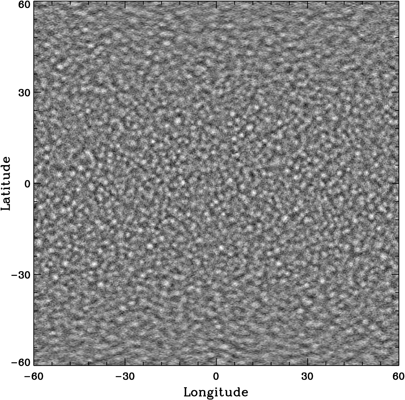
HMI observations have refined our understanding of supergranular flow patterns, their depth structure, and their relationship to magnetic field distributions. The time-distance helioseismology pipeline developed for processing the HMI data provides the subsurface flow maps covering in latitude and longitudes in the range of depth from 0.5 to 19 Mm every 8 hours (Zhao et al., 2012b). A sample of a small area of horizontal flow maps is illustrated in Figure 18, and the flow divergence over the whole area is shown in Figure 19. These maps reveal the interaction of supergranular convection with magnetic fields, particularly in the areas of active regions, where the supergranular convection is suppressed, and the flow pattern is dominated by larger-scale converging flows (Kosovichev and Zhao, 2016). However, these maps do not show the organization of supergranules in large-scale coherent structures.

In addition, the horizontal flow maps are obtained by the ring-diagram technique. Figure 20 shows the horizontal flow field and corresponding horizontal divergence maps at various depths (Greer, Hindman, and Toomre, 2016). This study also suggested that supergranulation does not form cell-like convective structures with a well-defined circular flow. Instead, the cell-like nature of supergranulation is only displayed in the horizontal dimensions at the photosphere. It was suggested that since the lifetime of supergranules is only a day or two, the convective pattern in a deep layer may not resemble the supergranulation at the surface.
The ubiquity of supergranulation in the HMI images opened new opportunities for studying the average supergranule by stacking and averaging thousands of individual supergranules. It was found that the magnetic field that congregates in the downflow lanes was significantly stronger (0.3 G) on the west (prograde) side compared to the east and that the intensity minimum to the east of supergranules was deeper than to the west, suggesting that this anisotropy was related to the wave-like properties of supergranules (Langfellner, Birch, and Gizon, 2018).
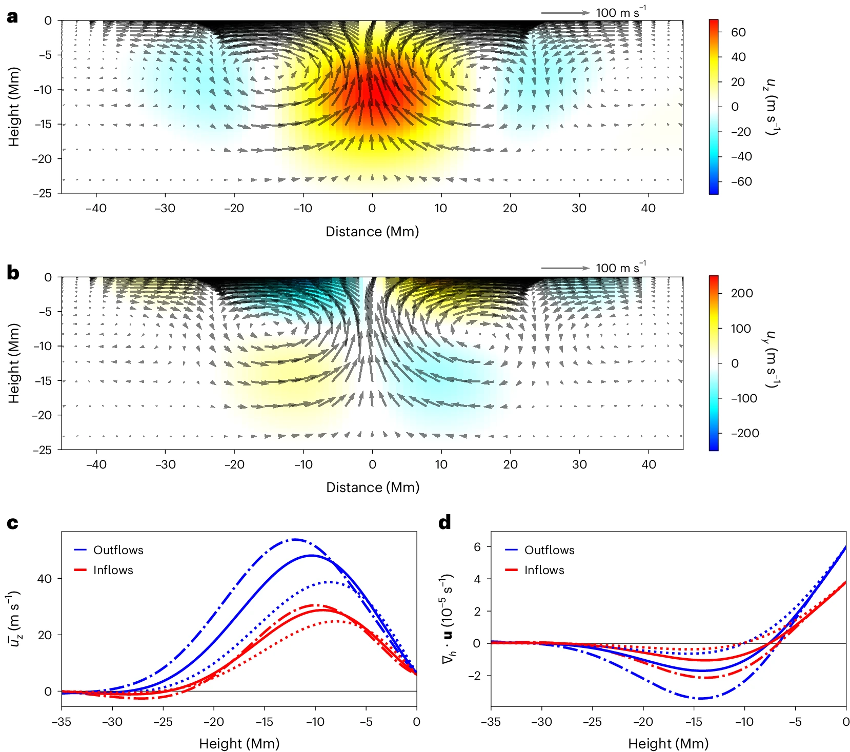
With the high signal-to-noise ratio that HMI provides, many helioseismic studies have attempted to probe the interior flows of supergranulation. Due to the weak vertical flows, many studies have relied upon mass-conservation arguments to infer the vertical flows that become more dominant at depth. In particular, analysis of time-distance measurements of the average supergranule suggested that supergranules were shallow, with peak upflows occurring a few Mm below the surface (Duvall and Hanasoge, 2013; Duvall, Hanasoge, and Chakraborty, 2014), and that supergranules extended at least to 7 Mm (Korda and Švanda, 2021). A new recent analysis of 23,000 supergranules, including full 3D flow inversions without relying on the mass-conservation constraint, found a peak upflow occurring at 10 Mm below the surface (Figure 21; Hanson et al., 2024). It was also noted that the peak upflow locations were invariant with the horizontal extent of supergranular-scale convection cells and that the downflow appeared to be 40% weaker than the upflows.
5.3 Detection of Giant Cells
The detection of convective giant cells with characteristic sizes of Mm is a much more challenging task. The velocities associated with the giant cells are small compared with granular and supergranular speeds and can hardly be isolated against the background of smaller-scale motions. The existence of such cells was predicted by Simon and Weiss (1968). Even before that, Bumba, Howard, and Smith (1964) noted indications of the presence of giant structures in the distribution of weak magnetic fields. However, giant cells were considered hypothetical for more than three decades. The earliest observational detection of giant cells was reported by Beck, Duvall, and Scherrer (1998), who computed correlation functions of Doppler images from the MDI instrument over many months. They reported the existence of large-scale east-west flows that persisted for months, which is in line with theoretical descriptions of giant-cell convection. However, the HMI ring diagram data showed that these signals might be dominated by active region inflows (Hanson et al., 2020).
Later, the presence of giant flow cells was revealed by tracking the motion of supergranules over many years (Hathaway, Upton, and Colegrove, 2013; Hathaway and Upton, 2021). It was found that the low-latitude cells have roughly circular shapes and lifetimes of about one month; they rotate nearly rigidly, do not drift in latitude, and do not exhibit any correlation between the longitudinal and latitudinal flow. The high-latitude cells have long extensions that spiral inward toward the poles and can wrap nearly completely around the Sun. They have lifetimes of several months, rotate differentially with latitude, drift poleward at speeds approaching m s-1, and have a strong correlation between prograde and equatorward flows. Spherical harmonic spectral analyses of maps of the divergence and curl of the flows confirm that the flows are dominated by the curl component with RMS velocities of about 12 m s-1 at wavenumber . It was noted that these large-scale flow patterns can be linked to the inertial convective modes. The structure of these flows with depth is currently unknown. However, similar large-scale spiral flow patterns were detected in 1 Mm deep subsurface layers by time-distance helioseismology (Zhao, 2016).
5.4 Spectrum of Solar Convection
Given the diverse spatial scales observed in solar surface flows, from granulation to giant cells, power spectra analysis has emerged as one of the most crucial tools for characterizing the properties of both surface and subsurface dynamics in the solar photosphere. This technique allows researchers to quantify the energy distribution across different scales, providing insights into the complex, multi-scale nature of solar convection (Rincon and Rieutord, 2018).
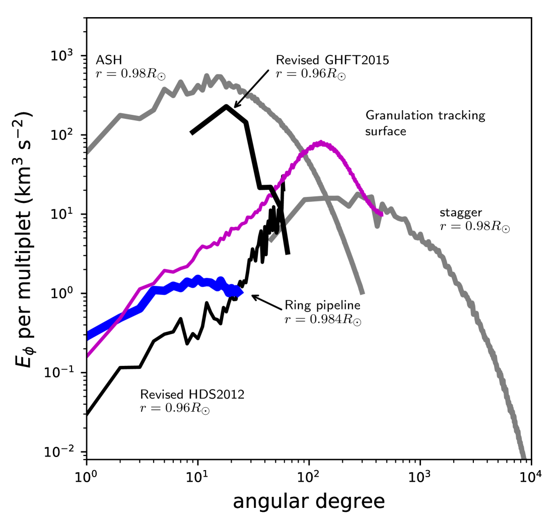
Figure 22 shows constraints obtained through a variety of techniques, reflecting the state of the art in both observations and numerical simulations, with the following caveats. The flow spectra in Figure 22 are at different depths and, depending on the type of measurement, may represent averages of flows over a depth range. For instance, supergranulation tracking uses the proper motions of supergranules to measure larger-scale flows; however, supergranules have finite extents in depth, implying that the inferred flow speeds are averaged over the supergranular depth range. Similarly, acoustic waves have radially delocalized eigenfunctions, which implies that the inferred flow speed is an integral of true convective flows with the wave eigenfunctions.
Hanasoge, Duvall, and Sreenivasan (2012) employed time-distance helioseismology to investigate convective velocity magnitudes in the near-surface shear layer at , examining them as a function of spherical-harmonic degree by representing the mean squared East-West convective velocity in terms of the parameter , defined as , where is the radius at which the flow field is measured. The curve labeled ‘Revised HDS2012’ in Figure 22 revealed smaller horizontal velocities at compared to the estimates from the numerical models of solar convection obtained from ASH simulations at (Miesch et al., 2012). These two results do not agree at any angular degree, though there is some overlap between the ASH simulation’s convective power spectrum and that of the Stagger simulations (Stein and Nordlund, 2006), also obtained at , for intermediate . The magnitude of the convective flows as derived from supergranulation tracking on the surface (Roudier et al., 2012) also overlap the ASH and Stagger spectra at certain points in the same range of angular degree and with the spectrum derived from the HMI ring diagram pipeline (Bogart, Baldner, and Basu, 2015) at low . At the lower end of the intermediate range—around —there does appear to be some agreement between the ‘Revised HDS2012’ and Stagger spectra, in addition to the spectra derived from the novel ring diagram pipeline developed by Greer et al. (2015). Despite some small overlap at specific angular degrees, the reason for the disagreements between each of these curves is not yet established and is currently a topic of debate and investigation.
Systematic comparisons between different observational techniques and simulations have highlighted the excess power in large convection scales. For instance, ring-diagram analysis has shown that the peak of the horizontal-velocity spectrum shifts to lower spherical-harmonic degrees with increasing depth, suggesting the presence of larger-scale velocity structures at greater depths (Greer et al., 2015).
An upper limit on the convective velocity at each spherical harmonic degree of at that follows from the energy spectra obtained by the time-distance technique and ring pipeline (Revised HDS2012 and Ring pipeline curves in Figure 22) is less than 3 m/s for convective motions. When summed over all spherical harmonic modes , this corresponds to an upper limit on velocity of less than 10 m s-1. This upper limit is more than an order of magnitude lower than the convective velocities predicted by mixing-length theory and found in global convection simulations.
This led to the convective conundrum statement: ‘The convective velocities required to transport the solar luminosity in global models of solar convection appear to be systematically larger than those needed to maintain the solar differential rotation and those inferred from solar observations (O’Mara et al., 2016). One suggested solution is the suppression of large-scale convective motions caused by solar rotation (Vasil, Julien, and Featherstone, 2021). This theory predicted that the dominant convection scale throughout the convection zone is about 30 Mm, which is the scale of supergranulation (the corresponding value is 100 – 120). It also suggested that supergranulation might be a manifestation of deep convection.
In this respect, a study of the spatial spectra of convective motions and their variation in the solar activity cycle showed an intriguing transition of the convective scales from supergranular to giant scales in the near-surface layer (Getling and Kosovichev, 2022).
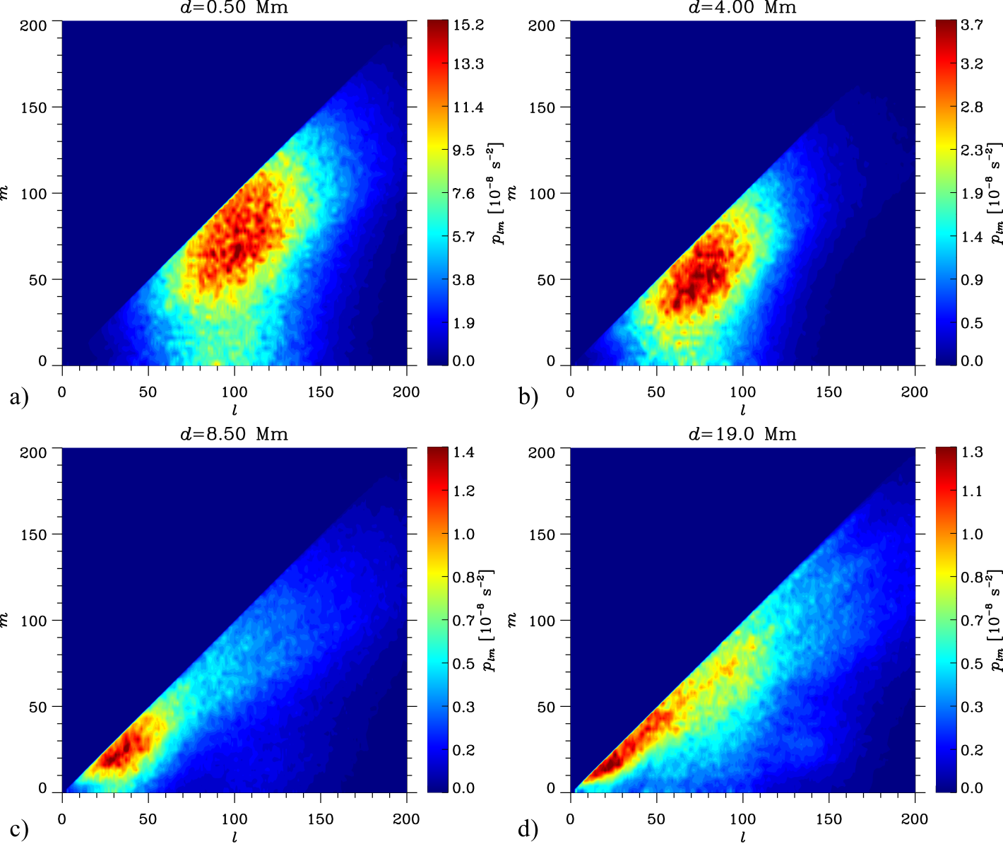
Figure 23 shows typical power spectra of the divergence field at various depths. In the upper layers, Mm, the spectrum peaked near degrees of , which corresponds to wavelengths of Mm; this is definitely the supergranulation scale. The peak is fairly wide in these shallow layers. As increases, the main spectral peak narrows and shifts toward low values or long wavelengths. In the deep layers, harmonics with , of scales Mm, are prominent, which appears to be indicative of the presence of giant cells.
It is remarkable that the spectral peak is very close to the line in the deep layer. Therefore, with the increase of , the most powerful harmonics become elongated in the meridional direction, approaching the sectorial structure (with a monotonic increase from the pole to the equator in each hemisphere at a given longitude). This seems to be an argument in favor of the repeatedly expressed idea of a banana shape of the global-scale convection structures (Glatzmaier and Gilman, 1981; Busse, 2002, etc.).
The supergranular-scale flows in the upper layers (, Mm) coexist with the upper parts of giant convection cells, whose presence is not pronounced there. However, the power values for the largest scales at the upper and deep levels are comparable.
The variation of the integrated spectral power of the flow during the activity cycle shows that while the total power is anti-correlated with the sunspot number at depths less than 4 Mm, it is positively correlated in the deeper layers. Such a behavior of the spectral power in the activity cycle can be interpreted based on the idea that the magnetic field, suppressing convection in the upper layers, redistributes its energy in favor of deeper layers. This agrees with the fact that converging flows observed around active regions may affect the convection spectra, as shown using the ring-diagram (Haber et al., 2004) and time-distance (Zhao and Kosovichev, 2004) techniques.
5.5 Flow Divergence and Vorticity
A non-spectral technique has been used to identify supergranules and measure the horizontal scale of supergranulation by estimating the supergranulation scale from horizontal flow divergence maps (see Rincon et al., 2017, and references within). According to the results of Getling and Kosovichev (2022) using HMI data, the horizontal flow divergence ranges from s-1 at a depth of 0.5 Mm to s-1 at a depth of 11.5 Mm.
The supergranular power spectrum of the divergence signal exhibits wave-like properties, indicating the presence of supergranular waves in surface horizontal flows near the solar equator (Gizon, Duvall, and Schou, 2003; Schou, 2003). Extension of the analysis to higher wavenumbers, corresponding to a spherical-harmonic degree larger than 120, showed an oscillation of the power spectrum with frequency of approximately 2 Hz, corresponding to waves with a period of about six days (Langfellner, Birch, and Gizon, 2018).
Due to the Coriolis force acting on diverging horizontal flows, solar supergranules exhibit a hemisphere-dependent preferred sense of rotation. Consequently, supergranules behave like weak anticyclones, with their vertical vorticity changing sign at the equator (Gizon, Duvall, and Schou, 2003). Using HMI data, it was further demonstrated that the correlation between vertical vorticity and horizontal divergence displays a latitudinal dependence consistent with the Coriolis force’s action on convective flows (Langfellner, Gizon, and Birch, 2014). In addition, a linear relationship between non-magnetic vorticities and divergences was reported in regions within latitude (Sangeetha and Rajaguru, 2016).
The analysis of both time–distance helioseismology and local correlation tracking to SDO/HMI data found that the typical vortical flow component is of the order of 10 m s-1 in the diverging core of supergranules, significantly weaker than the diverging horizontal flow component itself (Langfellner, Gizon, and Birch, 2015). The kinetic helicity proxy, defined as the dot product of velocity and its curl, exhibits a hemispheric pattern similar to vorticity. These flows possess negative kinetic helicity in the northern hemisphere and positive kinetic helicity in the southern hemisphere throughout most of the convection zone (Kosovichev and Zhao, 2016; Hathaway and Upton, 2021).
5.6 Current Challenges and Future Directions
Significant advancements in understanding and simulating solar convection have occurred over the past three decades. This progress stems from two main factors: significantly improved computational resources and continuous high-cadence observations of the full solar disk. These observations come from the ground-based Global Oscillation Network Group (GONG), and notably, space-based instruments like the Michelson Doppler Imager (MDI) and Helioseismic and Magnetic Imager (HMI). Since 2010, HMI has provided nearly continuous high-precision data with enhanced spatial resolution. These new data and the remarkable developments in helioseismology they spurred have enabled further insights into solar convective flows, as briefly presented in this section.
The Sun’s convective region extends approximately 200 Mm below the surface, where density varies by several orders of magnitude. Solar convection manifests across a broad spectrum of spatial dimensions and temporal scales. This complex and dynamic zone is characterized by intricate interactions between plasma motions and thermal gradients, which in turn interact with magnetic fields. This multi-scale complexity explains why many challenges remain in fully characterizing and understanding convective flows.
An outstanding challenge is ‘the convective conundrum’ - the discrepancy of one or several orders of magnitude in the kinetic energy as a function of angular degree, observed between different helioseismic techniques and types of analysis (Figure 22). The disagreement also exists between these observational results and the numerical simulations, and it varies with depth (Lord et al., 2014).
New emerging mode-coupling helioseismic techniques further highlighted this issue by reporting results that contradict numerical models (Woodard, 2006; Hanson and Hanasoge, 2024). They also found that downflows are significantly weaker than upflows, suggesting the presence of small, undetectable descending plumes that maintain mass-flux balance. This finding further challenges the validity of the mixing-length theory in explaining solar convection.
Giant cells are prominent in most global simulations, but another puzzling issue is that they appear to have a very weak signal in observations, making them difficult to detect. The recent discovery that many of these large-scale structures are actually inertial waves raises the question of which, if any, are actual giant convective cells. Interestingly, inertial modes are expected to provide additional constraints on the physics of the deep convection zone (Hotta et al., 2023).
Despite all the progress achieved, much remains to be done in both theoretical analysis and observational studies. The continuation of HMI data is highly desirable. Moreover, a new, improved HMI-like instrument with full-disk coverage, high cadence, high spatial resolution, and capability for long-term observations would significantly enhance our understanding of convective flows.
6 Differential Rotation
The main features of the solar rotation profile – the near-surface shear layer, differential rotation in the convection zone, and the shear layer or tachocline between the convection zone and the largely rigidly-rotating radiative interior – were already established before HMI was launched (Thompson et al., 1996; Schou et al., 1998). There were some discrepancies between the inferred rotation profiles from the two instruments, including a jet-like feature at 75 degrees latitude that was seen in inversions of MDI but not GONG data. These discrepancies were caused by differences in the mode fitting pipelines rather than the instruments; specifically, an anomaly in the MDI odd-order splitting coefficients around a frequency of 3.5 mHz and an underestimation of the low-degree rotational splittings in the GONG data (Schou et al., 2002).
Inversions of the first months of HMI rotational-splitting data showed a profile that resembled that seen in the MDI full-disk data, confirming that the high-latitude jet in the rotational inversions of the MDI data was an artifact (Howe et al., 2011). Further studies using an improved algorithm to estimate mode parameters from MDI and HMI determined that the systematic effects and the high-latitude jet feature were caused by the ‘vector-weighted’ binning of the MDI data, which was performed onboard the SoHO spacecraft to satisfy the telemetry requirements (Larson and Schou, 2018, 2024). This was confirmed by a rotational inversion that employed the high-degree modes in the range of angular degree from 0 to 1000 and the frequency range from 965 to Hz, obtained from the 66-day-long 2010 MDI Dynamics Run performed with full -pixel resolution (Reiter et al., 2020).
The picture of the global solar rotation given by HMI, therefore, is relatively simple, with the rotation rate varying rather smoothly with latitude.
6.1 Features of the Solar Rotation Profile
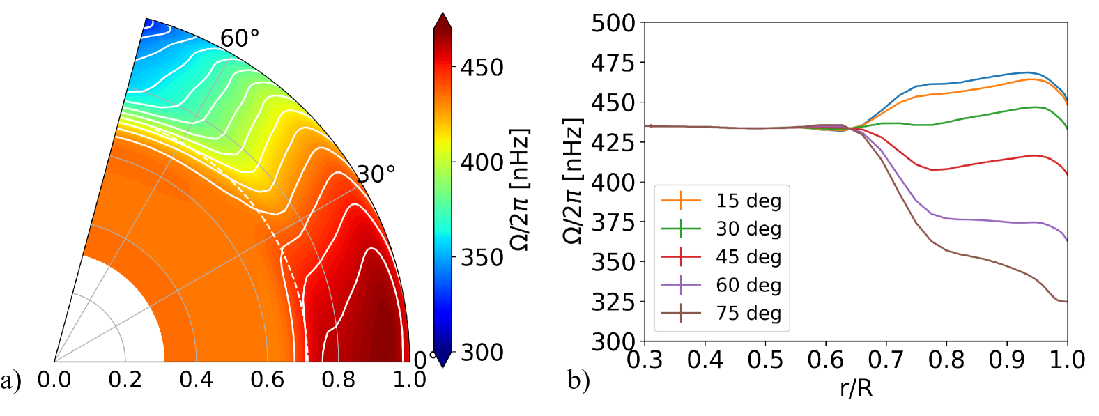
Figure 24 shows the mean rotation profile derived from the default HMI two-dimensional Regularized Least-Squares (2dRLS) inversions of rotational splittings up to that can be downloaded from the JSOC (data series hmi.V_sht_2drls). Below we discuss what had been learned from HMI observations about the main features of the rotation.
6.1.1 Near-Surface Shear Layer
The sharp decrease in the rotation rate in a shallow subsurface region (called the Near-Surface Shear Layer or NSSL), which is believed to play a crucial role in the solar dynamo (Charbonneau, 2010; Pipin and Kosovichev, 2011), has been in the focus of global and local helioseismology since its initial discovery (Rhodes et al., 1988; Korzennik et al., 1988). Of particular interest was a question whether the radial gradient of the rotation rate changes (and even changes sign) at higher latitudes, for which there was some evidence (e.g. Thompson et al., 1996; Kosovichev et al., 1997; Corbard and Thompson, 2002; Barekat, Schou, and Gizon, 2014; Rozelot, Kosovichev, and Kitiashvili, 2025).
Some other measurements found no indication of a reversal in the sign of the radial gradient (Rhodes et al., 1990; Corbard et al., 2013; Reiter et al., 2020). Although the HMI results in Figure 24 seem to indicate a change in the rotational gradient at about 70∘, this controversy has not been resolved because of the difficulties of resolving the structure of the solar differential rotation at high latitudes. It is worth noting that the analysis of Reiter et al. (2020) is the only one using global modes (from MDI) with degrees greater than 300.
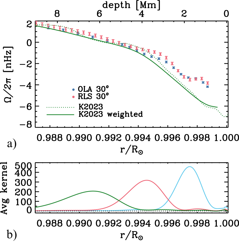
The ring-diagram analysis of Rabello Soares, Basu, and Bogart (2024) focusing on the NSSL regions along the central meridian and averaging over the 12-year observing period showed that the NSSL can be divided into three regions: a large layer below 0.994 (4 Mm) with a small shear where the radial gradient of the logarithmic rotation rate increases in amplitude from at 21 Mm to at 4 Mm; a narrow middle layer centered around 0.9965 (2.4 Mm) with a strong shear and a gradient of approximately ; and a narrow layer close to the surface from about 0.9977 (1.6 Mm) where the radial gradient is close to zero but becomes negative and steeper again toward the surface (Figure 25).A similar fine structure of the NSSL, which is about 10 Mm-thick (the so-called “leptocline”), was found in 3D radiative hydrodynamic simulations (Kitiashvili et al., 2023) and also in global helioseismology data (Rozelot, Kosovichev, and Kitiashvili, 2025).
In addition, a combined analysis of data from MDI, HMI, and GONG by Antia and Basu (2022) revealed that the shear layer is shallower at higher latitudes than close to the equator and varies with the solar cycle.
6.1.2 Tachocline
The thickness of the tachocline is much smaller than the horizontal resolution of inversions, sometimes estimated to be smaller by a factor of 10. Consequently, estimates of the thickness are done through forward modeling of the splitting coefficients rather than through inversions. Attempts are being made to improve the resolution of the inversions (Korzennik et al. in preparation) by using iterative methods to measure tachocline properties through inversions. Early results were obtained by modeling the second odd-order splitting coefficient ( or ), which shows the largest signature of the tachocline (Kosovichev, 1996a; Basu, 1997). Later, a variety of optimization techniques were used to determine the tachocline parameters as a function of latitude (Antia, Basu, and Chitre, 1998; Charbonneau et al., 1999). These results and later ones showed that (i) the tachocline is prolate in shape, with the midpoint of the change in rotation occurring below the convection-zone base at low latitudes and in the convection zone at mid and high latitudes, and (ii) the change in the rotation rate occurs over a very narrow range of radii, and that this thickness is latitude-dependent. More recent results obtained with HMI data (Basu and Antia, 2019) confirm this.
6.1.3 Radiative Interior
The rotation profile of the region below the tachocline cannot be resolved in as much detail as the regions near the surfaces. In general, the observations are believed to be consistent with uniform rotation. It is important to be aware of systematic errors when looking for deviations from this uniformity. The uncertainties in measuring parameters of low-angular-degree modes that are sensitive to the solar core rotation are reduced when longer time series and better mode-fitting methods are used (Korzennik, 2005, 2008). While the multi-instrument analysis of observational data from HMI, MDI, GONG, and the Birmingham Solar-Oscillations Network (BiSON) indicates consistency with a rigidly rotating solar core at 431 nHz, the results did not rule out a faster or a slower rotation rate for (Eff-Darwich and Korzennik, 2013). Although the radiative zone rotates rigidly, a systematic dip evolving with time was noted at and 60∘ latitude in both MDI and GONG data. This feature has not been confirmed by the HMI data.
6.2 Summary
The application of both local and global techniques to HMI data has improved our understanding of the Sun’s rotation profile, particularly in the near-surface layers where recent studies have uncovered the detailed structure of the near-surface shear layer in both depth and latitude (Rabello Soares, Basu, and Bogart, 2024). Developments in high-degree global helioseismic fitting (Korzennik et al., 2013; Reiter et al., 2020) hold promise for further exploring these shallow layers. At greater depths, inversions of HMI data confirm the prolate shape of the tachocline (Basu and Antia, 2019) and the near-uniform rotation in the radiative interior (Eff-Darwich and Korzennik, 2013).
7 Meridional Circulation
7.1 Brief Introduction
The Sun’s meridional circulation is the global-scale interior flow in the Sun’s meridional plane.Although it is an order of magnitude weaker than differential rotation – about m s-1 at the surface and only a few m s-1 in the deeper convection zone – it plays an important role in solar dynamo and interior dynamics. The meridional transports magnetic flux and redistributes angular momentum (e.g., Wang, Nash, and Sheeley, 1989; Miesch, 2005; Upton and Hathaway, 2014a, b; Featherstone and Miesch, 2015). Its speed was also reported to correlate with the duration and strength of solar cycles (Hathaway and Rightmire, 2010; Dikpati et al., 2010).
Over the past three decades, advancements in helioseismology, using data from GONG, MDI, and HMI, have significantly improved our understanding of the Sun’s meridional circulation. While early studies focused primarily on meridional flow near the surface, the detection of deep meridional flow throughout the solar convection zone became more feasible with the advent of HMI observations. High-resolution continuous data from HMI have provided valuable information on the flow’s structure, depth, and temporal variations, although the profile of the deep meridional flow remains a subject of debate. This section presents a brief review of recent studies on the structure of meridional circulation. The solar-cycle variations are discussed in Section 9.
7.2 Surface and Sub-Surface Meridional Flow
The meridional flow on the solar surface and subsurface (a few tens of megameters below the surface) has been intensively investigated and well-recognized by early studies before HMI. Various studies have consistently measured a poleward flow on the order of m s-1, achieved by methods such as surface Doppler measurements (e.g. Duvall, 1979; Hathaway, 1996), surface feature tracking (e.g. Howard and Gilman, 1986; Komm, Howard, and Harvey, 1993; Švanda, Zhao, and Kosovichev, 2007), time-distance helioseismology (e.g. Giles et al., 1997; Zhao and Kosovichev, 2004), ring-diagram analysis (e.g. González Hernández et al., 1999; Haber et al., 2000), and Fourier-Legendre analysis (e.g. Braun and Fan, 1998; Krieger, Roth, and von der Lühe, 2007; Doerr et al., 2010). HMI, with its higher resolution, has enabled measurements of surface meridional flow up to higher latitudes using local helioseismology methods and extended the study of the long-term evolution of meridional circulation during the solar cycles.
7.2.1 Observational Results from HMI
HMI pipeline products provide subsurface flow maps derived from ring-diagram methods (Bogart et al., 2011a, b) and time-distance method (Zhao et al., 2012b) (see Section 3.2 for more details). From these data, the meridional flow was obtained and its long-term temporal evolution was studied (Zhao, Kosovichev, and Bogart, 2014; Komm et al., 2015; Komm, Howe, and Hill, 2018; Lekshmi, Nandy, and Antia, 2019; Komm, Howe, and Hill, 2020; Getling, Kosovichev, and Zhao, 2021). Figure 26 shows the one-year-average meridional flow profiles at Mm for the first three years of HMI observations, where the largest meridional flow speed occurs at low latitudes near 20∘. The latitude of the faster meridional flow is observed to migrate toward lower latitudes, as depicted in Figure 42 in Section 9.2.3, which shows the residual meridional flow after removing a long-term mean profile. In mid-latitude areas, an anti-correlation between the meridional flow speed and the magnetic flux was reported for Solar Cycle 23. The temporal evolution of the near-surface meridional flow will be further discussed in Section 9.2.3.
7.2.2 Polar Meridional Flow
Surface and subsurface meridional flows are routinely measured by HMI observations up to about latitudes, but the polar meridional flow remains a missing piece in helioseismology. Observational evidence of counter cells (equator-ward flow) in the polar regions was reportedly found using non-helioseismology methods, such as correlation tracking with MDI and HMI data (Ulrich, 2010; Hathaway and Rightmire, 2010; Hathaway, Upton, and Mahajan, 2022; Ulrich, Tran, and Boyden, 2022) and surface flux transport simulations with Hinode data (Yang et al., 2024). However, the counter-cell detection is sporadic and shows no clear solar-cycle dependence.
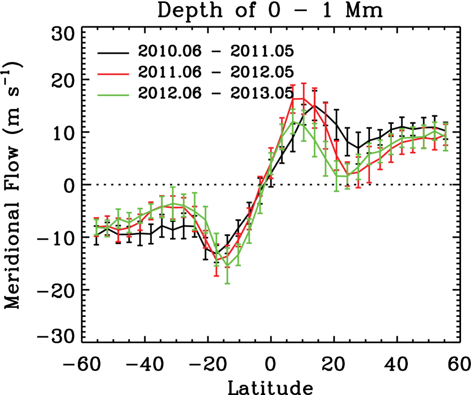
7.3 Deep Meridional Flow
While the surface and subsurface meridional flows have been widely studied with consensus, determining the deep meridional flow remains challenging, as the p- and f-mode oscillations are more sensitive to the outer layers of the convection zone than the deeper interiors. Studies have provided inconsistent results, leaving key questions—such as the number of circulation cells in the Sun’s radial direction and the depth of the equatorward return flow—still open for debate.
Although the interior rotation profile across the convection zone has long been established, the meridional flow cannot be determined using the same global helioseismology techniques of measuring frequency splitting since the frequencies of global p-modes are not sensitive to meridional circulation to the first order. Instead, the deep meridional circulation has primarily been studied using local helioseismology techniques, particularly the time-distance method (Section 3.2). Multiple research groups have measured the meridional flow throughout the entire convection zone, but their findings remain inconsistent, largely due to many systematic effects complicating these measurements. In this subsection, we will discuss the results and the ongoing challenges in time-distance measurements. Additionally, a few other techniques, such as Fourier-Legendre decomposition and normal-mode coupling, have been explored to measure deep meridional flow, and we will briefly review these next.
7.3.1 Deep Meridional Flow Measured by Time-Distance Method
Analysis of HMI data showed that the travel time measurements for large travel distances that are required for measuring flows in the deep convection zone are affected by systematic errors that could be misinterpreted as a flow along the limb-to-center direction (Zhao et al., 2012a; Chen and Zhao, 2018). Known as the center-to-limb (CtoL) effect, it increases with both measurement depth and the center-to-limb position. Figure 27 illustrates this effect from the HMI data in comparison with the meridional-flow-induced signals (Chen and Zhao, 2017). The travel time shift caused by this effect can be 5 – 10 times larger than the flow-induced travel times. Therefore, its removal is critical for determining the deep meridional flow.
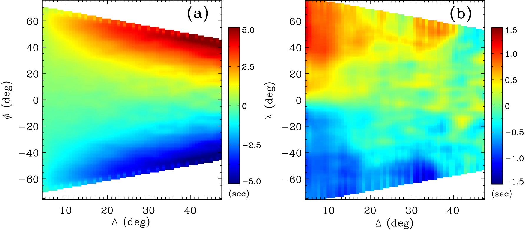
.
The physical mechanism of the systematic center-to-limb frequency shift is yet to be established. It could be caused by near-surface convective flows (Baldner and Schou, 2012), changes in the spectral line formation height (Kitiashvili, Couvidat, and Lagg, 2015), or by non-adiabatic effects contributing to the observed Doppler shift (Waidele, Zhao, and Kitiashvili, 2023). An empirical method proposed to remove the shifts uses measurements along the East-West direction in the equatorial region (Zhao et al., 2013). After applying the correction, this study showed that the meridional flow has a double-cell structure along the radius in the convection zone. It is directed from the equator to the poles in the top Mm layer and at the base of the convection zone, but between (from 65 to 125 Mm beneath the solar surface, or from 0.82 R⊙ to 0.91 R⊙, the meridional flow is equatorward (Figure 28a).
However, subsequent analyses by different research teams, following similar measurement methods with various modifications, yielded mixed results regarding the detailed circulation profile. A study using GONG observations supported the presence of shallow return flow but reported a single-cell circulation pattern with a weak double-cell structure at low latitudes (Figure 28b; Kholikov, Serebryanskiy, and Jackiewicz, 2014; Jackiewicz, Serebryanskiy, and Kholikov, 2015). A follow-up inversion using the same observations confirmed the shallow return flow but found the number of cells inconclusive due to the inversion’s sensitivity to regularization parameters (Böning et al., 2017). Another measurement using HMI observations and inversions with a mass-conservation constraint reported a single-cell circulation in each hemisphere (Figure 28c; Rajaguru and Antia, 2015; Mandal et al., 2017). Meanwhile, a study using 15 years of MDI medium- data revealed a double-cell circulation during solar minima and a temporal variation of the circulation pattern with solar cycles in low-latitude regions (Figure 28e; Liang and Chou, 2015; Lin and Chou, 2018). All the above measurements used the same proxy method to remove the CtoL effect. This empirical approach was validated by a comprehensive study that measured along all disk radial directions (Chen and Zhao, 2017). The study demonstrated that HMI’s CtoL effect is isotropic with respect to the azimuthal angle, confirming the effectiveness of the simpler proxy method. Using this more robustly determined CtoL effect, the study revealed a double-cell meridional circulation pattern (Figure 28d).
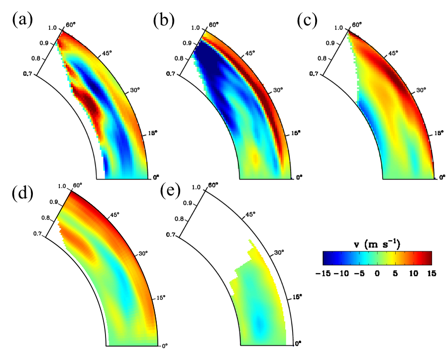
Recent studies have employed multi-instrument measurements to determine the meridional circulation. A forward modeling of combining data from MDI and HMI favored a single-cell meridional circulation (Liang et al., 2018). Another study, based on only GONG and MDI data, showed a single-cell meridional circulation throughout Solar Cycles 23 and 24, with a possibility of a weak second cell at low latitudes in the southern hemisphere from 2005–2011 (Gizon et al., 2020). Additional studies that applied a Bayesian inversion method (Jackiewicz, 2020) on these multi-instrument measurements indicated the meridional circulation in Solar Cycle 23 exhibited a strong single-cell profile, while in Cycle 24, it had a weak poleward flow component reaching nearly zero in the middle of the convection zone, which might indicate a double-celled structure (Herczeg and Jackiewicz, 2023). It was also shown that the meridional flow structure inferred by the inversion of the observed acoustic travel times depends on the flow constraints implemented in the inversion procedures – applying an angular momentum transport constraint changed the inverted profile from a single-cell to a double-cell configuration (Hatta, Hotta, and Sekii, 2024). Numerical simulations of the travel-time measurements found that the high noise levels of stochastically excited solar oscillations make it difficult to definitively distinguish between single-cell and double-cell structures through observations alone (Stejko, Kosovichev, and Pipin, 2021).
7.3.2 Other Methods
A different method (Fourier-Legendre decomposition) that included a control measurement designed to assess and remove the center-to-limb effect applied to 88 months of HMI data indicated significant hemispheric differences: the meridional flow found equatorward at approximately 40 Mm below the photosphere in the northern hemisphere while remaining poleward in the southern hemisphere (Braun, Birch, and Fan, 2021).
7.4 Summary
The ongoing research continues to focus on understanding these systematics and refining observational methods, showing promise for further advancements in measurements. Simulations and inversions also emphasize the need for improved measurement precision to resolve ambiguities in deep flow inversion. Different techniques and constraints in inversions have yielded varying circulation profiles, and some simulations indicate that current measurement precision may be insufficient to definitively distinguish between single-cell and double-cell circulations.
8 Solar Inertial Waves
8.1 Introduction
Waves propagating through the Sun’s interior can be classified based on their restoring forces. Acoustic waves (p-modes) are restored by pressure gradient forces and excited by turbulent convection. Internal gravity waves (g-modes) are waves restored by buoyancy and mainly propagate through the convectively stably-stratified radiative zone. Both acoustic waves and gravity waves are relatively high-frequency modes, oscillating with periods of several minutes and several hours, respectively. In addition to these, inertial waves (including Rossby waves or r-modes) that are driven by the Coriolis force and oscillate very slowly with periods of several months were also believed to exist in the Sun (Provost, Berthomieu, and Rocca, 1981; Saio, 1982; Unno et al., 1989; Dziembowski and Kosovichev, 1987b). Detecting such low-frequency modes required long-term observational data with sufficient signal-to-noise ratios spanning many years, which was achieved using the HMI observing series.
The observations have revealed several types of inertial waves, including equatorial Rossby waves (Löptien et al., 2018), high-latitude and critical-latitude modes (Gizon et al., 2021), and high-frequency retrograde modes (Hanson, Hanasoge, and Sreenivasan, 2022; Gizon et al., 2024). The frequencies of these modes in the Carrington rotation rate as a function of the azimuthal wavenumber , and examples of the mode eigenfunctions obtained from observations and a theoretical model (Bekki, Cameron, and Gizon, 2022b; Bekki, 2024) are shown in Figure 29. Properties of these modes are discussed in detail in Sections 8.2 and 8.3.
8.2 Equatorial Rossby, Critical-latitude, and High-Frequency Retrograde (HFR) Modes
A special class of inertial modes is Rossby waves or r-modes, whose motions are quasi-toroidal, i.e., the radial motions are very small compared to the horizontal ones (Papaloizou and Pringle, 1978; Pedlosky, 1987; Rieutord and Valdettaro, 1997). They propagate in a retrograde direction (opposite to the rotation) in a co-rotating frame.

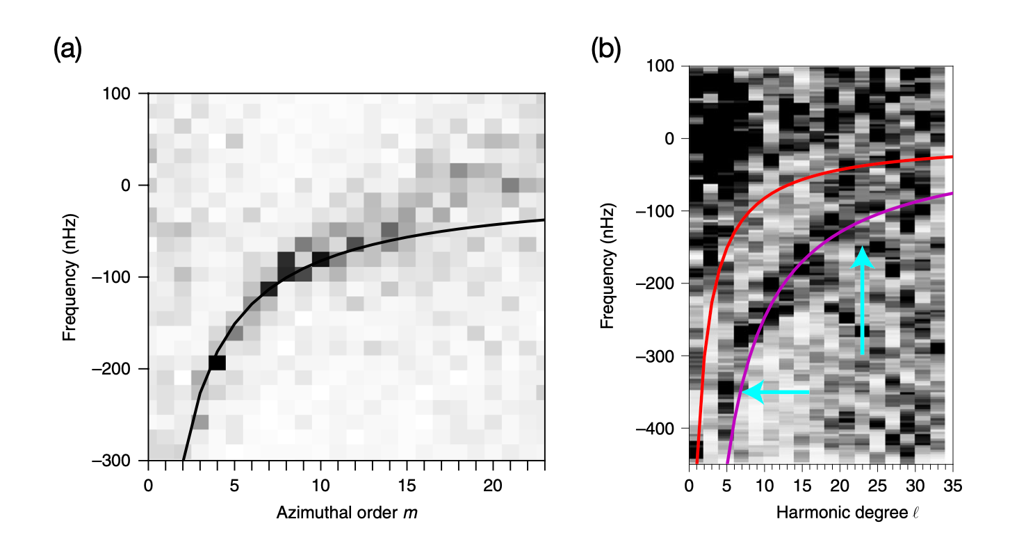
Different methods have been utilized to detect these modes. The initial observation of solar inertial modes was obtained by tracking the motion of granules in intensity images from HMI and also by using subsurface flow maps from the ring-diagram technique. Evidence of the equatorial Rossby waves was found from six years of HMI data (Figure 30a). It was found that the sectoral () component of radial vorticity power for the range of dominantly lies along with the theoretical dispersion relation of the Rossby waves (Papaloizou and Pringle, 1978; Provost, Berthomieu, and Rocca, 1981; Saio, 1982):
| (2) |
where is the temporal frequency, is the azimuthal order, is the spherical harmonic degree, and nHz is taken as the equatorial rotation rate of the Sun. Since the sectoral modes have radial vorticity, which peaks at the equator and decreases at higher latitudes, they are also called equatorial Rossby waves. They have typical velocity amplitudes of m s-1 at the surface and lifetimes of several months.
The characteristics of the equatorial Rossby waves have since been corroborated by multiple studies employing various techniques, including the normal mode coupling technique (Hanasoge and Mandal, 2019; Mandal and Hanasoge, 2020; Mandal, Hanasoge, and Gizon, 2021), time-distance helioseismology (Liang et al., 2019), the ring-diagram technique (Hanson, Gizon, and Liang, 2020; Proxauf et al., 2020) and local correlation tracking of features (supergranules) (Hathaway and Upton, 2021). These studies characterized the frequencies, linewidths, and amplitudes of the Rossby modes for the azimuthal order up to using HMI data products (Bhattacharya et al., 2024; Hanson and Hanasoge, 2024). The Rossby mode with azimuthal order is not observed; only an upper limit of 0.2 m s-1 on its amplitude has been placed (Mandal, Hanasoge, and Gizon, 2021).
The measurements of the latitudinal eigenfunctions (Löptien et al., 2018; Proxauf et al., 2020; Mandal and Hanasoge, 2024) showed that they differ from the spherical harmonic predicted by theory in the case of uniform rotation (Provost, Berthomieu, and Rocca, 1981). A more general theory of low-frequency oscillations predicted that the latitudinal eigenfunctions of Rossby (r) modes can be represented in terms of eigenfunctions of the Laplace tidal equation (Dziembowski and Kosovichev, 1987a). In addition, the r-modes are strongly affected by the differential rotation and, in particular, the critical latitudes where the phase speed of the Rossby waves is equal to the differential rotation speed. At such latitudes, the energy exchange between the flow and waves causes the coupling of the spherical harmonics, resulting in the mode instability and a wave continuum spectrum (Dziembowski and Kosovichev, 1987b).
In fact, dozens of modes whose eigenfunctions are strongly concentrated near their critical latitudes were found using ten years of HMI data (see, Figure 29: Gizon et al., 2021). Although the mode power peaks at the critical latitudes, the power excess at the mode frequency can be seen over the entire latitude range. Frequencies of the observed critical-latitude modes cannot be represented by a well-defined dispersion relation. In such cases, the eigenfunctions are sensitive to the internal properties of the Sun, such as viscosity. It was shown that the latitudinal widths of the critical layers are controlled by turbulent viscosity (Gizon, Fournier, and Albekioni, 2020). Further, 3D models imply that substantial radial motions are involved, which makes them also sensitive to the superadiabaticity (Dziembowski and Kosovichev, 1987a), particularly, near the critical latitudes (Gizon et al., 2021).
In addition to the equatorial () modes, a distinct power ridge corresponding to the mode was detected in the near-surface radial vorticity power spectra (Figure 30b; Hanson, Hanasoge, and Sreenivasan, 2022). The waves would appear as anti-symmetric vorticity patterns about the equator, in contrast to the equatorially symmetric Rossby modes. The detected power ridge does not follow the theoretical dispersion relation of the classical Rossby waves given by Equation (2). These modes propagate in a retrograde direction at frequencies about three times faster than those of equatorial Rossby modes. Given these circumstances, the detected modes were called “high-frequency retrograde (HFR)” modes. Theoretical studies imply that these HFR modes are essentially non-toroidal, involving substantial radial motions near the equator (Triana et al., 2022; Bhattacharya and Hanasoge, 2023; Bekki, 2024; Jain, Hindman, and Blume, 2024; Blume, Hindman, and Matilsky, 2024).
While the latitudinal profile is well constrained by the observations, the variations with depth are more elusive. The eigenfunctions of the equatorial Rossby waves deduced from the ring-diagram analysis up to 15 Mm below the surface (Proxauf et al., 2020) deviated from the theoretical eigenfunctions calculated for the uniform rotation and inviscid limit (Provost, Berthomieu, and Rocca, 1981; Dziembowski, Kosovichev, and Kozlowski, 1987). A recent theoretical study found that viscous diffusivity has a significantly greater impact on the radial structure of Rossby waves (Bekki, Cameron, and Gizon, 2022b). The mode-coupling technique has the capability to detect the signal up to a depth of (Mandal and Hanasoge, 2024). However, the radial structure of the mode eigenfunctions has not been established.
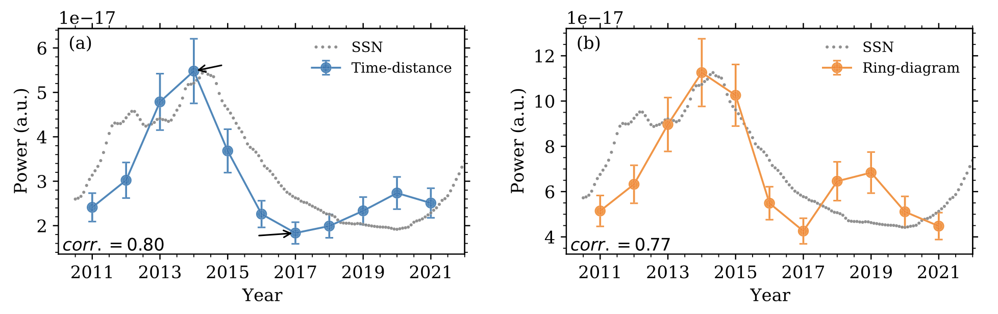
Figure 31 presents an analysis of 12 years of inferred subsurface velocity fields derived from the SDO/HMI time–distance and ring-diagram pipelines. The results show that the Rossby wave amplitude is higher during the solar activity maximum than during the minimum, while the frequency of Rossby waves is lower during the maximum than during the minimum (Waidele and Zhao, 2023; Lekshmi et al., 2024). This is opposite to the first-order predictions that considered only perturbations due to torsional oscillations (Goddard et al., 2020).
It raises questions about the excitation mechanism of Rossby waves. It was suggested that, similarly to p-modes, Rossby modes are stochastically excited by convection (Dziembowski, Kosovichev, and Kozlowski, 1987; Philidet and Gizon, 2023). The calculated amplitude is about 1 m s-1, in good agreement with the observations (Gizon, Fournier, and Albekioni, 2020). These modes are also present with significant amplitudes in nonlinear simulations of rotating convection (Bekki, Cameron, and Gizon, 2022a; Matilsky et al., 2022; Blume, Hindman, and Matilsky, 2024). The role of magnetic activity on these modes should be investigated numerically to better understand their variations with the solar cycle.
8.3 High-Latitude Modes (Polar Spiral Flows)
Global-scale spiral velocity patterns around the poles (above ), which persist for several months and move retrograde with respect to the Carrington rotation rate at high latitudes, were found by tracking the motions of supergranules seen in HMI Doppler observations (Hathaway, Upton, and Colegrove, 2013). They have a dominant flow component at azimuthal order , which corresponds to the high-latitude velocity pattern previously found in Mt. Wilson Observatory (MWO) Dopplergrams (Ulrich, 1993, 2001). Similar polar spiral flow patterns were found in subsurface flows using the ring-diagram analysis (Bogart, Baldner, and Basu, 2015).
These spiral flows can represent high-latitude inertial modes because their retrograde propagation frequencies are in the inertial frequency range of the Sun (red points in Figure 29a) and the associated power excess characterized by a single frequency can be seen at all latitudes (Gizon et al., 2021). The mode is of particular interest because it has the largest time-averaged amplitudes at the surface ( m s-1) among all the observed solar inertial modes. A recent study using the normal mode coupling technique found that this mode extends (almost uniformly in radius) all the way to the base of the convection zone (Mandal and Hanasoge, 2024). It was also found that the mode amplitude is stronger during the solar minimum than in the maximum (Figure 32, Gizon et al., 2024; Liang and Gizon, 2024). These new observations imply that the high-latitude inertial modes are substantially influenced by internal dynamo-generated magnetic fields. Theoretical models showed that the high-latitude modes are baroclinically-unstable by the latitudinal entropy gradient and have a significant impact on the Sun’s differential rotation (Bekki, Cameron, and Gizon, 2024). The readers may also refer to a recent review (Gizon et al., 2024).
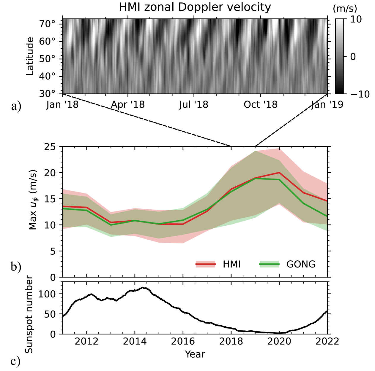
8.4 Conclusion
Various inertial modes have been successfully observed on the Sun. Having Coriolis force as their restoring force, these inertial modes have many unique properties that are not possessed by conventional acoustic modes. Theoretical models show that they are sensitive to some currently unknown parameters of the Sun, such as turbulent viscosity and superadiabaticity, both of which are poorly constrained by conventional acoustic-mode helioseismology. The detection of a large number of unique inertial modes hints at the possibility of “inertial-mode helioseismology”, potentially revealing new insights into the deep interior of the Sun. Furthermore, the sensitivity of inertial modes to the global scale magnetic fields may push forward our understanding of the solar dynamo. In the future, further analysis of observational HMI data (in tandem with other instrumental data) and improvement of theoretical models will deepen our understanding of solar inertial modes, which will help us to infer the convective properties and magnetic fields hidden deep in the Sun.
9 Solar Cycle Variations and Dynamo
A precise knowledge of the variability in the solar interior is important for understanding the origin of magnetic activity and constraining dynamo models. After the discovery of solar acoustic oscillations in the early 1960s (Leighton, Noyes, and Simon, 1962), the first results on their variability came in the mid-1980s. Woodard and Noyes (1985) reported a decrease in the frequencies of 0.42 Hz between 1980 and 1984 using the low- Active Cavity Radiometer for Irradiance Monitoring data. Since then, a large number of studies have been carried out to improve the characterization of global modes and to explore the changes in the inferred parameters, such as the oscillation frequencies, the mode line widths, and amplitudes, with varying solar activity. In addition, helioseismic observations have been widely used to study solar-cycle variations of the internal rotation and large-scale subsurface flows.
In this section, we give an overview of results obtained primarily from the HMI observations and how they compare with the contemporaneous observations of other instruments.
9.1 Solar-Cycle-Related Changes in Acoustic Mode Parameters and Splittings
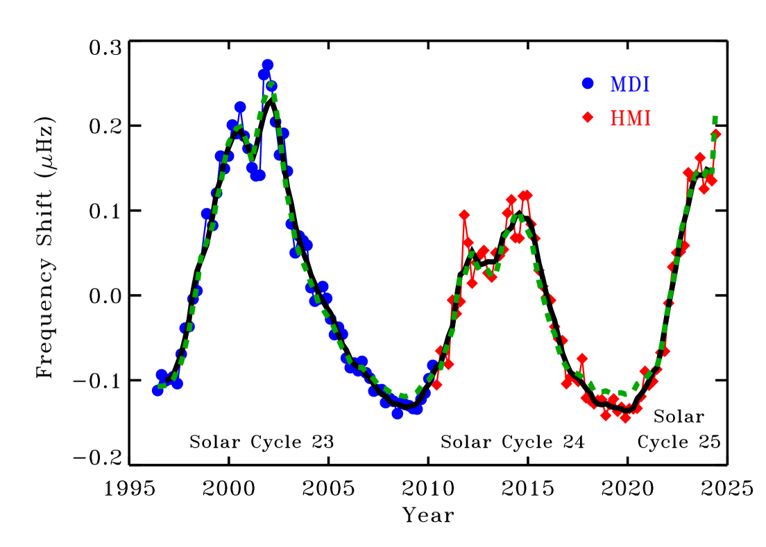
Figure 33 displays the temporal variation in p-mode frequency shifts from MDI and HMI observations starting from 1 May 1996. These shifts are calculated using common modes between all 141 datasets in the frequency range of 1500-4500 Hz, each derived from 72 d of observations, with the first 71 datasets from MDI111111jsoc.stanford.edu/ajax/lookdata.html?ds=mdi.vw_V_sht_modes and the remainder from HMI121212jsoc.stanford.edu/ajax/lookdata.html?ds=hmi.V_sht_modes. The MDI and HMI data are considered together as a continuous set, and the frequency shifts are scaled by mode inertia. The dashed line in the figure depicts the variation of solar activity represented by the 10.7 cm radio flux131313www.spaceweather.gc.ca/forecast-prevision/solar-solaire/solarflux/sx-5-en.php. It is clear that the frequencies vary in the phase of the solar cycle and show a strong positive linear correlation between them (Pearson’s correlation coefficient is 0.99). These findings are consistent with the previous studies (see Jain et al., 2012; Basu, 2016; Jain et al., 2022, and references therein). Similar results were found for f-mode frequencies, which were further utilized to study the changes in solar seismic radius and their implications on the total solar irradiance (Jain, Tripathy, and Hill, 2018; Kosovichev and Rozelot, 2018). In addition, as shown in Figure 34, there is a strong dependence in frequency shifts, which is reduced by scaling with the mode inertia, and the obtained frequency shifts provide true variations in frequencies.
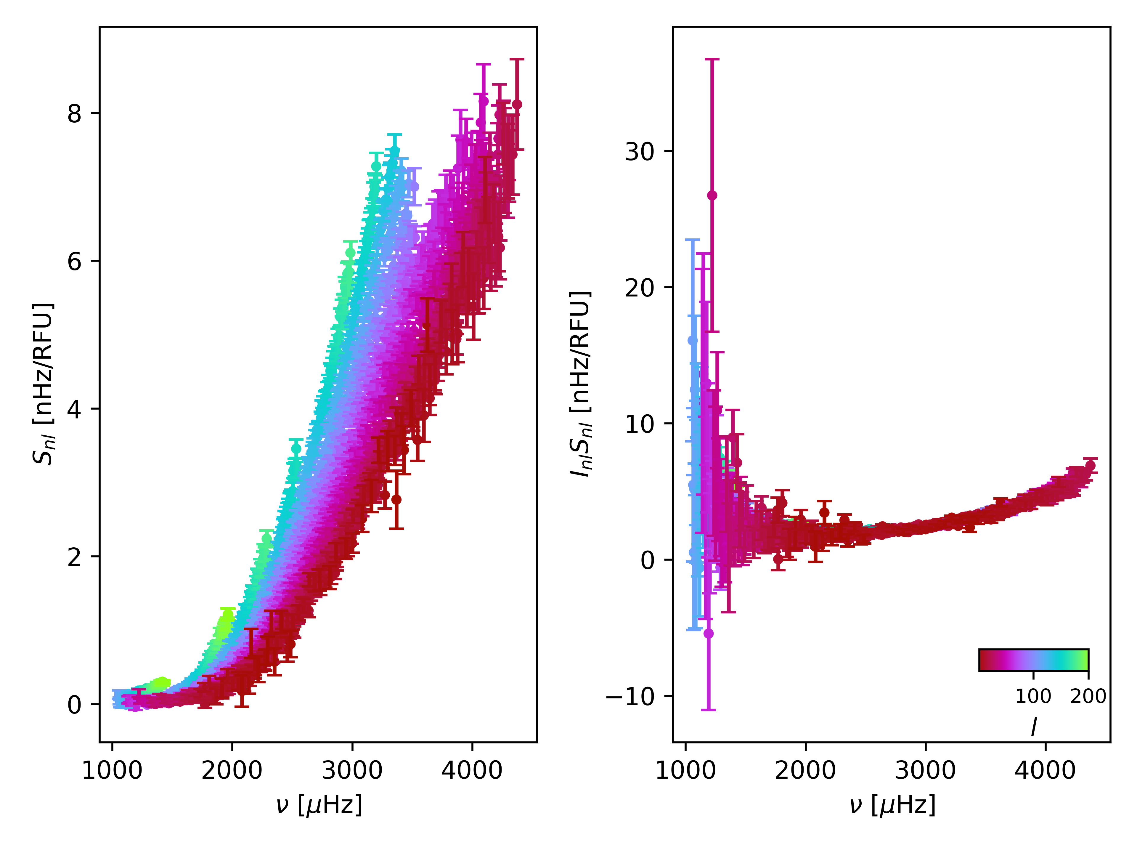
The relative variation in the global oscillation frequencies observed by HMI with the change in solar activity has been studied and compared with those from other instruments, e.g., MDI and GONG, by several authors (Jain et al., 2013, 2016; Howe et al., 2018a; Rabello Soares, 2019). All these studies showed comparable results indicating that the sensitivity of the oscillation frequencies to the change of magnetic activity does not vary significantly with the choice of instrument and is similar for the same phase of solar cycles. However, the correlation between the frequency variations and the solar radio flux deviates from a linear relation during the very high activity period, suggesting a saturation effect in the oscillation frequency variations (Rabello Soares, 2019).
The progression of the Solar Cycle 24 is studied by analyzing high- acoustic mode frequencies in localized regions derived from the technique of ring diagrams141414jsoc.stanford.edu/HMI/Rings.html using HMI full-resolution Dopplergrams (Undzis, Tripathy, and Jain, 2019). The authors confirm that these frequencies are strongly correlated with the changes during the solar cycle and display a strong correlation on spatial as well as temporal scales. It was found that the frequency variations in the Northern hemisphere peaked before the Southern hemisphere, which is consistent with the findings obtained by analyzing frequencies from GONG (Baird, Tripathy, and Jain, 2024) and the measures of magnetic activity. The temporal variations in the amplitudes and widths of high-degree acoustic modes from GONG, MDI, and HMI measurements during the declining phase of Solar Cycle 23 and the rising phase of Cycle 24 were similar for all three instruments. However, the variations in Cycle 24 were smaller than in Cycle 23 because of the weaker magnetic activity (Burtseva et al., 2013).
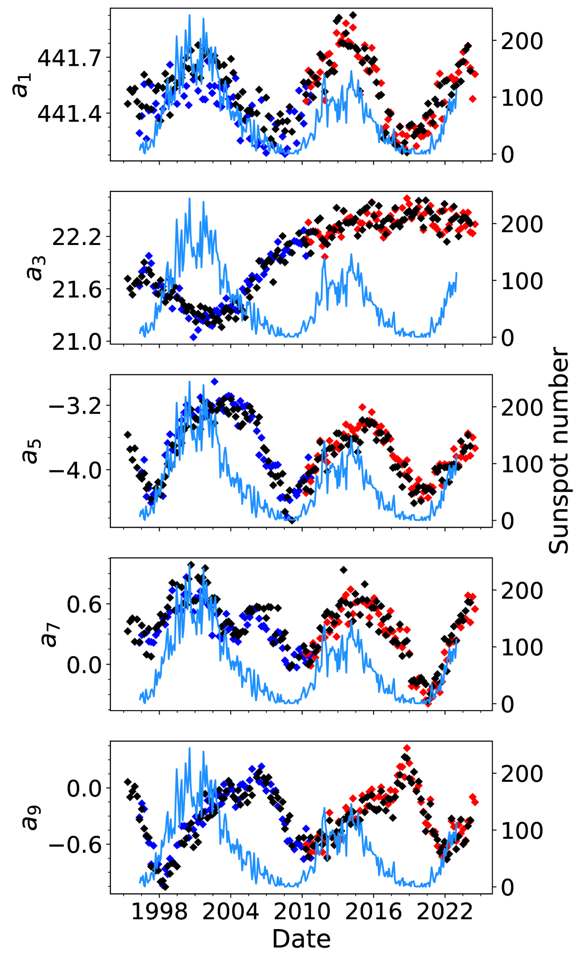
The odd-order splitting coefficients, characterizing latitudinal components of the solar differential rotations, shown in Figure 35 from all three instruments, revealed complex variations with the solar cycles (Korzennik, 2023). While the coefficient, , describing a latitudinally averaged component, displays an 11-year cyclic pattern in phase with the sunspot number, the other coefficients are either out of phase or do not follow any systematic variations. Since these coefficients are used to measure rotation rate, their amplitude and phase variations indicate changes in the internal solar rotation during Solar Cycles 23, 24, and 25 (see Section 9.2.1).
9.2 Solar-Cycle Variation of Subsurface Flows
Both the solar rotation (zonal flow) and the meridional flow vary over the solar cycle. The variation in the rotation rate that manifests in the pattern of migrating bands of faster and slower rotation known as the ‘torsional oscillations’ first discovered in Doppler observations of solar rotation (Howard and Labonte, 1980) is now continuously monitored by helioseismic instruments: GONG (1995 to present), MDI (1996 – 2011) and HMI (2010 to present). The flows were reported in early MDI f-mode data (Kosovichev and Schou, 1997), and they were subsequently shown to penetrate deep into the convection zone (e.g., Howe et al., 2000; Vorontsov et al., 2002). The near-surface meridional flow has also been found to be modulated by solar activity, with bands of converging flow associated with the magnetic activity belts (e.g., Zhao and Kosovichev, 2004). The continuously available high-resolution helioseismic observations from HMI have allowed more detailed study of these phenomena during Solar Cycles 24 and 25, revealing the extended 22-year cycle in the variations of the zonal flows and meridional circulation (Komm, Howe, and Hill, 2018; Getling, Kosovichev, and Zhao, 2021; Mahajan, Sun, and Zhao, 2023).
In a different approach, the subsurface zonal and meridional flows were measured by applying the ring-diagram technique to Dopplergrams constructed from the HMI global spherical harmonic coefficients. The preliminary results agree with the traditional ring-diagram analysis near the surface and intermediate depths, but the measured meridional flow in the depth range of Mm is reversed compared to the flows observed near the surface (Tripathy et al., 2024).
9.2.1 Zonal Flows
Zonal flows appear as a modulation of the solar rotation rate and can be inferred by making a data cube of successive two-dimensional rotation-rate inferences and then subtracting a temporal mean at each latitude and depth. When using inversions of global modes, this provides only the equatorially symmetric part of the pattern; to see the anti-symmetric component, we need to use results from local helioseismology. Figure 36 shows the zonal-flow measurements at a target depth of from MDI and HMI observations. The equatorward-migrating branches associated with Solar Cycles 23, 24, and 25 are clearly visible, while the behavior at higher latitudes is somewhat less regular. Similar results are obtained from the local helioseismology techniques (Figure 37).
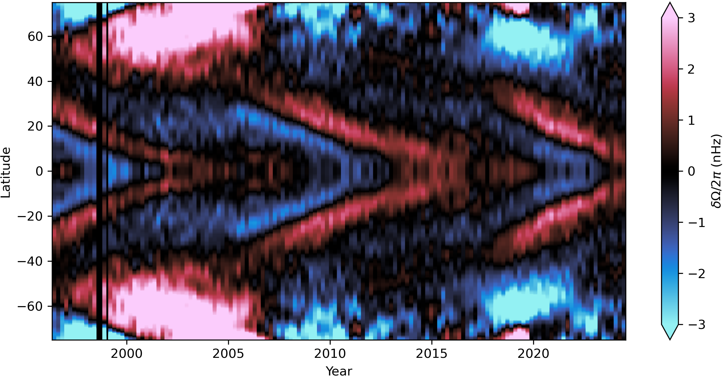
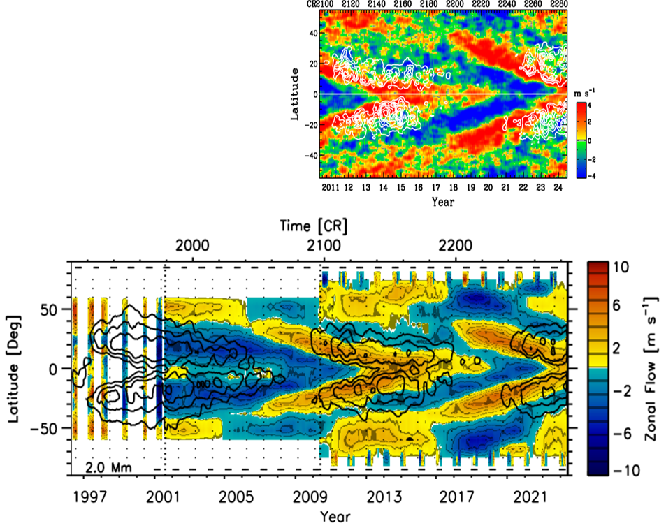
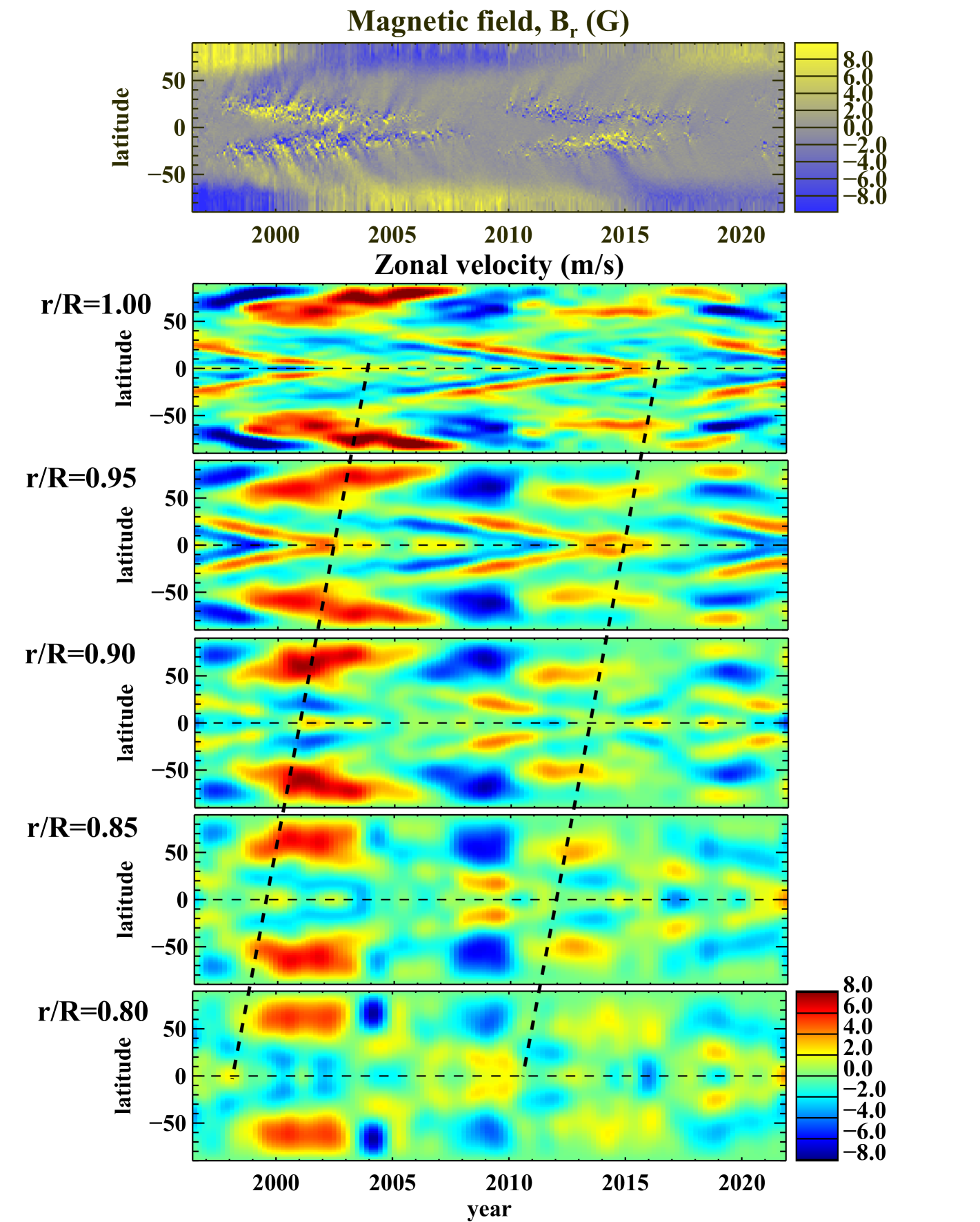
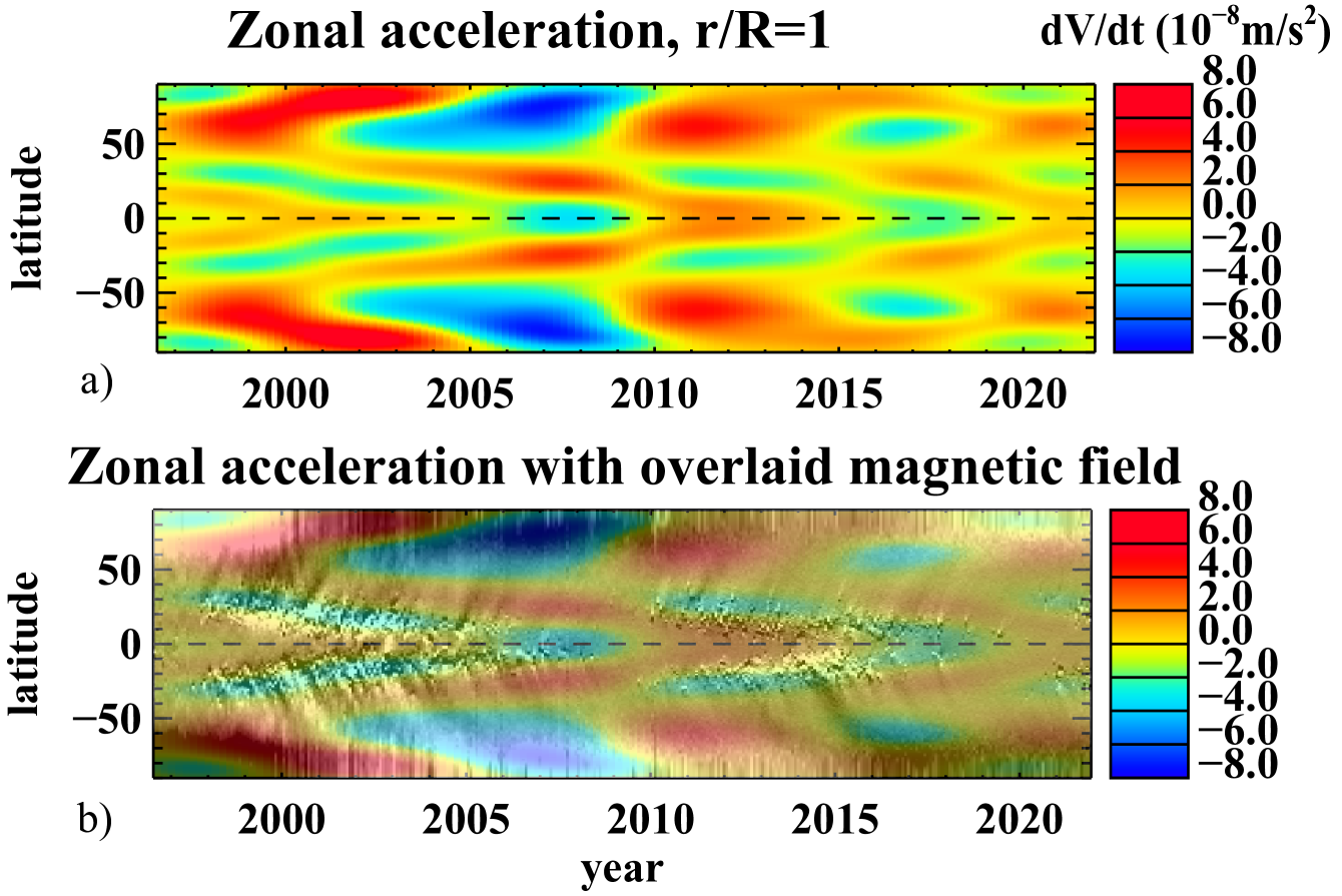
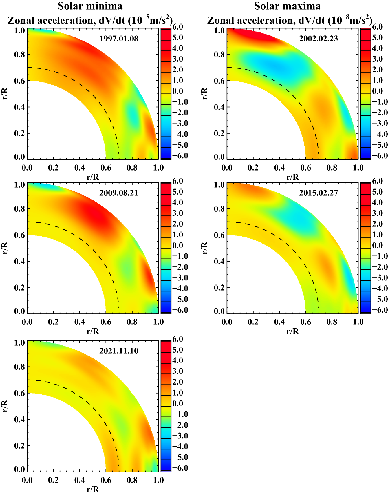
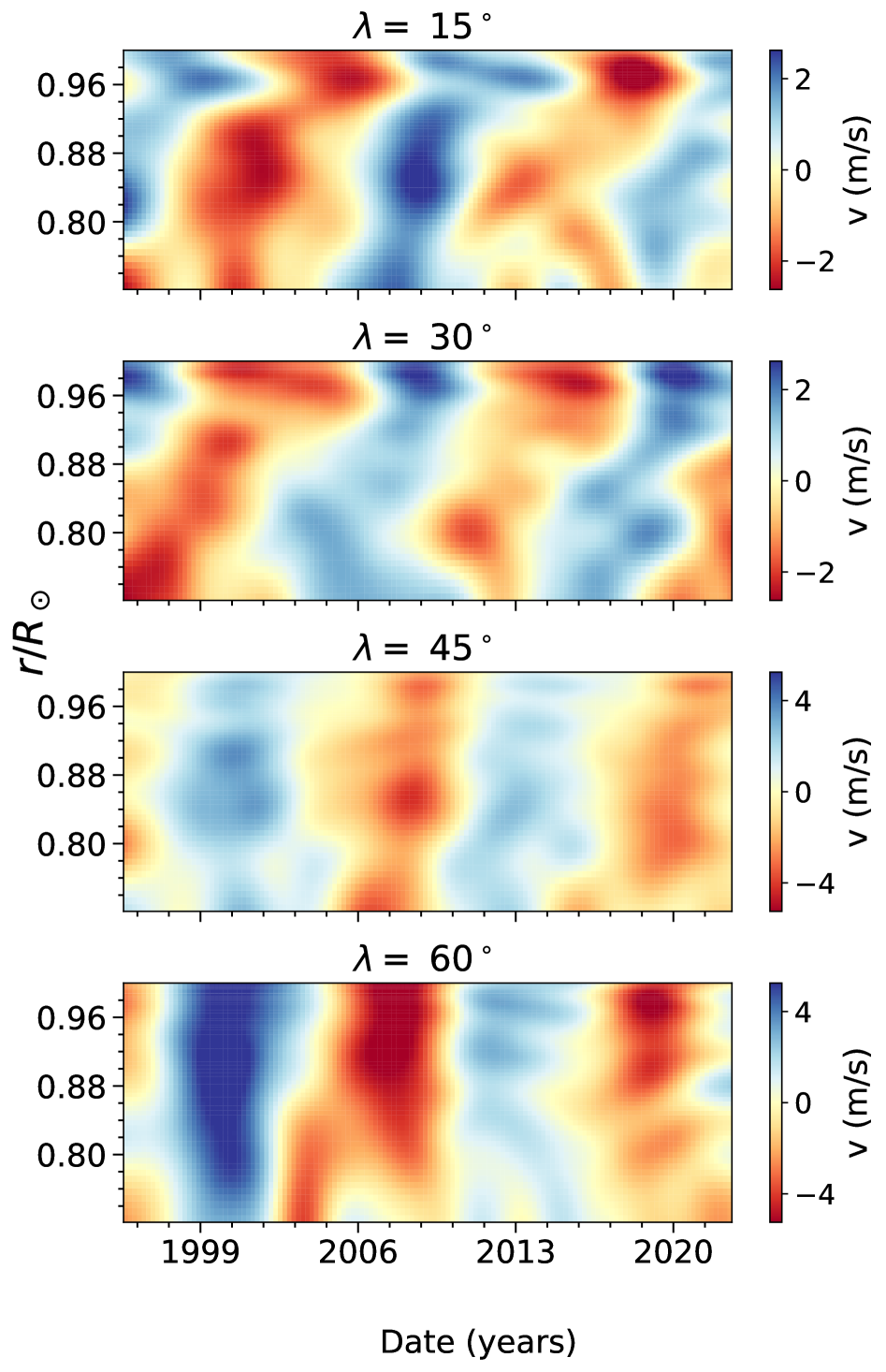
Subtracting a temporal mean over the whole data set, which now covers multiple solar cycles, can cause some problems because the “underlying” rotation rate may not be the same as the temporal mean over the available observations. Initial measurements of the torsional oscillations incorporating the HMI data (Howe et al., 2013) found a substantially weaker appearance of the high-latitude branch of the pattern corresponding to Solar Cycle 24 compared to this branch observed in Solar Cycle 23, but much of this appearance can be explained by the slower underlying rotation rate in Cycle 24. This slowing-down of the mean rotation rate at the high latitudes could result from weaker polar fields in Cycle 24, as suggested by a flux-transport model (Rempel, 2012), which showed that a reduction in the cycle amplitude leads to a drop in the high-latitude rotation rate. By 2018, with nearly two full cycles of data, the relative slow-down in the higher-latitude rotation for Cycle 24 was even more apparent, while the beginning of the equatorward branch of the torsional oscillation pattern for Cycle 25 was visible at mid-latitudes (e.g. Howe et al., 2018b; Basu and Antia, 2019).
The hemispheric asymmetry in the solar-cycle evolution of the zonal and meridional flows was initially detected by the time-distance helioseismology analysis using the first 3.7 years of data acquired by SDO/HMI during the rising phase of Cycle 24 (Zhao, Kosovichev, and Bogart, 2014). A ring-diagram analysis with tiles to examine both zonal and meridional flows in HMI observations revealed that the band of faster zonal flow associated with Cycle 25 appeared first in the northern hemisphere. In the range of depths covered by this analysis, down to about 32 Mm below the surface, the zonal flows appeared almost simultaneously (Komm, 2021). However, a global helioseismology analysis that provides measurements of the zonal flows through the whole convection zone (Figure 38) indicated that the flow bands in the deeper layers appear earlier than in the subsurface layers (Kosovichev and Pipin, 2019) and the time lag of the polar branches is shorter than that of the equatorial branches (indicated by dashed lines in Figure 38. These flow maps were obtained by subtracting the mean rotational velocities observed by the MDI and HMI instruments from the individual 72-day measurements and then smoothing the variation with a one-year window function.
However, for understanding the physical mechanism of the zonal flows and comparison with models, it is beneficial to consider the zonal acceleration (Kosovichev and Pipin, 2019) or the rate of change of the rotation rate (Mahajan et al., 2024). Comparison of the time-latitude diagram of the zonal acceleration calculated for a near-surface layer with the photospheric magnetic field map (Figure 39) showed that the magnetic field regions at low and high latitude coincide with the regions of zonal deceleration. Tracing the evolution of the zonal acceleration with the solar cycle (extracted from the observed variations of the zonal flows by applying a Principal Component Analysis) revealed a pattern of waves originating near the bottom of the convection zone and traveling in radius and latitude (Figure 40; Kosovichev and Pipin, 2019). Two basic wave branches were identified, a relatively fast high-latitude (polar) branch that reaches the surface in 1 – 2 years and an equatorial branch that takes about 11 years to reach the surface (Figure 41; Mandal, Kosovichev, and Pipin, 2024). It is intriguing that the data in this figure show a special role of the near-surface shear layer, in particular, reverse migration of the flow pattern from the surface to the bottom of this layer, indicating that the solar dynamo generates magnetic field not only in the deep convection zone but also the near-surface layer.
9.2.2 Temporal Variation of the Near-Surface Shear Layer
As the amplitude of the zonal flow varies with depth, it might be expected that the gradient of the near-surface shear will also show cycle-related changes as the torsional oscillation moves through it. In fact, however, recent studies suggest that changes in the near-surface shear are related more directly to the latitudes of magnetic activity. The variation of the near-surface shear layer in f-mode data from the 360-day MDI and HMI power spectra during Solar Cycle 23 showed an increase in the steepness of the gradient in phase with the solar cycle at low latitudes (Barekat, Schou, and Gizon, 2016). In addition, Antia and Basu (2022), using a combination of f-mode and p-mode data, found that the radial gradient increases in steepness with increasing solar activity at 0.990 and decreases in steepness at 0.950 during Solar Cycles 23 and 24. The changes are more pronounced in the active latitudes than at adjoining higher latitudes. Results at high latitudes of about 70∘ and poleward are unreliable. The NSSL is deeper at lower latitudes than at high latitudes, with a maximum at the equator. The extent of the NSSL also varies with the solar cycle. More recently, Rozelot, Kosovichev, and Kitiashvili (2025) found that the radial gradient of solar rotation is enhanced in the latitudinal zones of sunspot and active region formation. In middle and low latitudes, the gradient enhancements below the leptocline follow the magnetic butterfly diagram. However, in the leptocline, the latitudinal patterns of the enhanced gradient are more complicated, resembling the overlapping ‘extended’ solar cycles of the torsional oscillations.
Local helioseismic techniques, such as ring-diagram analysis, (for example, Zaatri and Corbard, 2009) also found that the radial gradient of the rotation rate in the NSSL varies with the solar cycle. In particular, in regions with strong magnetic flux, the radial gradient decreases (in magnitude) close to the surface at 0.997 (2.0 Mm) but increases in deeper layers at 0.990 (7.0 Mm) (Komm, 2022b; Antia and Basu, 2022), suggesting that the solar-cycle effects on the shear were likely to reflect the “presence or absence of magnetic flux above a certain threshold.” In addition, the thickness of the NSSL varies with the solar cycle: it extends to about 0.952 (29.4 Mm) at locations of active regions compared to 0.956 (35.3 Mm) at those of quiet regions (Antia and Basu, 2022; Komm, 2023).
9.2.3 Meridional Flow Modulation
The ring-diagram and time-distance analyses of the solar-cycle variation of the meridional flow showed a similar pattern to the torsional oscillation, with bands of converging meridional flow moving from mid- to low latitudes during the solar cycle (Komm, 2021; Getling, Kosovichev, and Zhao, 2021). At latitude, these bands were found to appear earlier at greater depths, apparently taking about two years to rise through the outer layers of the convection zone from the 32 Mm depth, but at lower latitudes, they appear almost simultaneously at all depths.
Figure 43 displays the time variations of the meridional (South-North) flow and the deviations from the mean revealing migrating bands in meridional flows, obtained by the time-distance method (Getling, Kosovichev, and Zhao, 2021). Apparently, the meridional flow variations reveal the extended solar-cycle structure originally found in the zonal flows. It is particularly apparent from Figure 42, which combines the data obtained from GONG, MDI, and HMI by the ring-diagram technique. Similarly to the zonal flows, the near-surface meridional flow showed a hemispheric asymmetry correlated with the asymmetry of magnetic activity, leading the activity by about three years (Lekshmi, Nandy, and Antia, 2019).
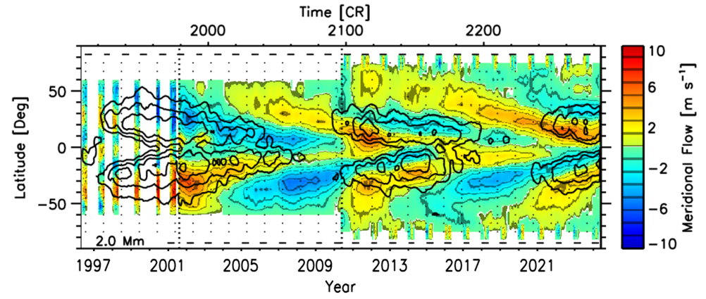
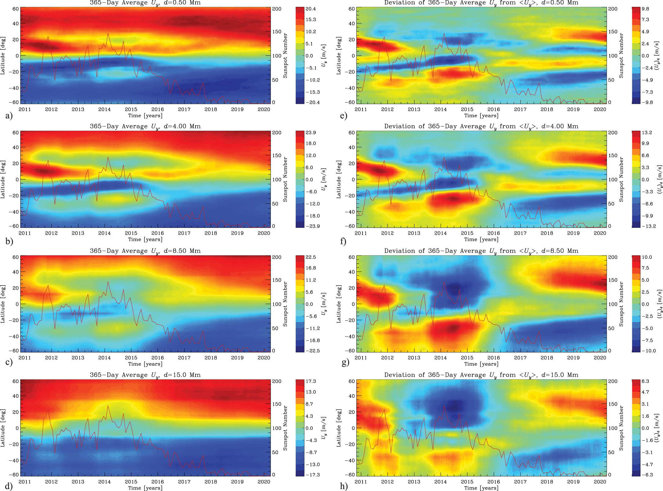
These results show that the meridional flow is significantly disturbed during the solar activity maxima, resulting in a substantial decrease in the flow speed from mid-latitudes to the polar regions and even the appearance of flows across the solar equator (Komm, Howe, and Hill, 2020), which may affect magnetic flux transport.
While at least some of the solar-cycle modulation of the near-surface meridional flow can be attributed to inflows into active regions, several studies have found that the active regions cannot account for the full observed effect. The contribution from active regions was found to be quite shallow, with maximum strength at 3.1 Mm depth (Komm, Howe, and Hill, 2020), while the solar-cycle variations of the meridional flow extend much deeper. In addition, excluding active region areas did not completely remove these variations, leading to a suggestion that the meridional flow is made up of three components: 1) active-region inflows, 2) a variation of about 2 m s-1 on solar-cycle timescales that cannot be attributed to active regions, and 3) the quiet-Sun background meridional flow (Mahajan, Sun, and Zhao, 2023).
The surface meridional flow and its variations have been studied by tracking the movement of the Sun’s magnetic network during the period May 1996 through May 2022 (Hathaway, Upton, and Mahajan, 2022). The results suggested that the meridional flow disappears above about 80∘ latitude and polar counter cells, i.e., equatorward flow from the poles down to about latitude, appearing from time to time, in general agreement with previous helioseismology results (Komm et al., 2013). However, more work is needed to confirm both findings.
9.3 Structural Changes in the Solar Convection Zone
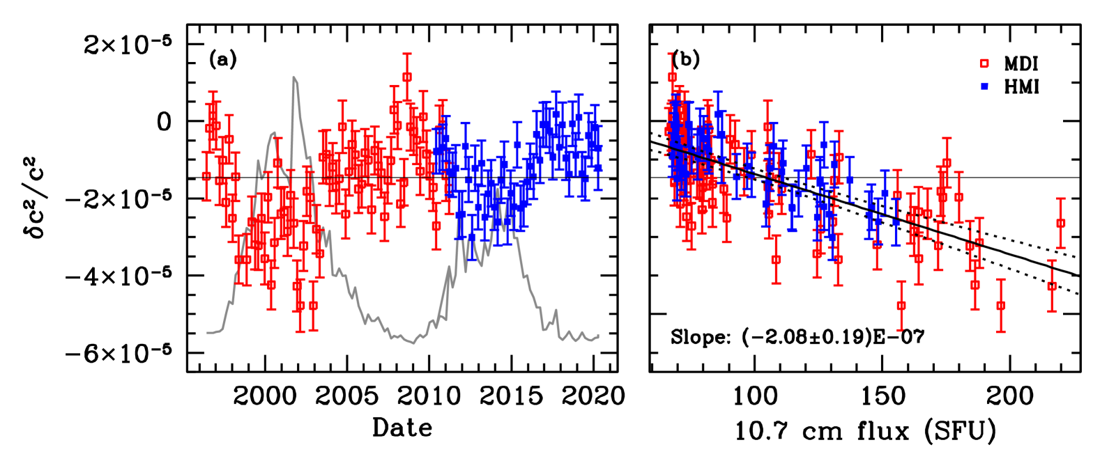
Analysis of the sound-speed variations in the solar interior between the activity minimum and maximum of Solar Cycle 23 using global helioseismology data revealed a two-layer configuration in the sound-speed difference, reminiscent of the structure observed beneath active regions (Figure 6 in Rabello-Soares, 2012). Near the surface (around 5.5 Mm depth), the sound speed at solar maximum was found to be lower than at solar minimum. This difference decreased until about 7 Mm depth, beyond which the trend reversed. In deeper layers (7-10 Mm), the sound speed at maximum became higher than at minimum, with the relative difference peaking around 10 Mm depth. The magnitude of this deeper positive difference was less than half of the negative difference observed near the surface. These results are consistent with predictions of a magnetic convection model, which considers the magnetic inhibition of convection onset in the presence of a vertical magnetic field (Mullan, MacDonald, and Rabello-Soares, 2012). However, it is important to note that the interpretation of these results is not straightforward. The observed changes in mode frequencies can be attributed to both structural changes in the medium through which the waves propagate and direct effects of magnetic fields on the plasma waves via the Lorentz force (Rabello-Soares, 2012) or reflect a combination of structural and non-structural effects of the magnetic fields (Lin, Li, and Basu, 2006).
Unlike the very clear changes in solar dynamics, changes in solar structure are small and difficult to detect. Helioseismic data obtained during Solar Cycle 23 hinted at changes in the second helium ionization zone (Basu and Mandel, 2004) and the base of the convection zone (Baldner and Basu, 2008), but these were not confirmed until HMI data showed that the changes could be seen in Solar Cycle 24 (Watson and Basu, 2020). This analysis showed that there is indeed a change in the layers that correspond to the He II ionization zone, which must be due to temperature changes in that layer. The time variation is easily discernible because the helioseismic data sets used covered two solar cycles.
In addition, small changes, of the order of a few parts in in the of the Sun just below and just above the base of the convection zone (Figure 44) were detected by sacrificing spatial resolution in favor of the temporal resolution (Basu, 2021). These changes are anti-correlated with solar activity, i.e., the sound speed is higher at the solar minimum than at the solar maximum. There also appears to be a change in the gradient of the sound speed at the convection-zone base, which could be an indication that the position of the base changes with activity. While there is some evidence that the radial location of the base of the convection zone has a slight latitude dependence, evidence of the time variation of this asphericity is marginal (Basu and Korzennik, 2024).
9.4 Quasi-Biennial Oscillations
In addition to the 11-year cyclic patterns, shorter quasi-periodic variations are also found in the helioseismic data. These variations, commonly known as quasi-biennial oscillations (QBOs), with periods ranging from 1.5 to 4 years, were initially identified in low- frequencies from the integrated-light instruments (Fletcher et al., 2010), but later found in the intermediate- frequencies from GONG (Jain, Tripathy, and Hill, 2011) too. Subsequent studies using helioseismic data from various sources, including HMI, support these findings (e.g., Simoniello et al., 2013; Mehta et al., 2022), and also reported two different QBO periods, about 2 years in Cycle 23 and 3 years in Cycle 24 (Jain, Chowdhury, and Tripathy, 2023). Inceoglu, Howe, and Loto’aniu (2021); Bogart et al. (2023) studied the presence and spatio-temporal evolution of QBOs in the rotation-rate residuals in NSSL and showed the QBO-like signals in each latitudinal band and depth; however, their amplitudes increase with increasing depth, suggesting the source region of the QBO to be below 0.78 . It is worth mentioning that QBOs are not limited to the helioseismic data only; they are also present in various activity indices and have been widely discussed in numerous papers.
The origin and periods of QBOs have been a subject of debate, and several mechanisms have been suggested. For instance, two dynamo sources separated in space give rise to two different periods (Benevolenskaya, 1998). The first source of the dynamo is located near the bottom of the convection zone responsible for the 11-year cycle, while the second source operating near the top in the near-surface shear layer could give rise to short-term periodicities. While some studies based on the helioseismic data suggest that the magnetic field responsible for quasi-periodic variations is anchored within the NSSL (Fletcher et al., 2010; Mehta et al., 2022; Jain, Chowdhury, and Tripathy, 2023), there are arguments that QBOs could arise from the beating between two types of magnetic configuration of the solar dynamo (Simoniello et al., 2013), or from an interplay between the flow and magnetic fields (Inceoglu et al., 2019).
9.5 Implications for Solar Dynamo Theories
All manifestations of solar activity, from solar irradiance variations to solar flares, are caused by the Sun’s magnetic field. This magnetic field is believed to be generated by a dynamo mechanism operating in the Sun’s convection zone (Parker, 1955), deep below the solar surface, although proposals exist for the near-surface origin of the Sun’s magnetic field (Vasil et al., 2024). Despite substantial modeling and simulation efforts, our understanding of how the magnetic field is generated, transported to the solar surface, and forms sunspots remains very limited.
Currently, we cannot measure subsurface magnetic fields by helioseismology. Thus, any knowledge about the dynamo process within must be gathered from measuring large-scale subsurface flows, such as differential rotation and meridional flow. It is expected that the 11-year sunspot-cycle evolution of subsurface magnetic fields modulates these flows via magnetic stresses, variations in turbulent heat transport, and inertial forces. Therefore, analyzing the solar-cycle-scale variations in zonal and meridional flows provides us with a way to peek into the heart of the solar dynamo.
Numerous explanations have been proposed for the measured variations in zonal flow (torsional oscillation) ranging from Lorentz forces (Schüssler, 1981; Covas et al., 2000; Guerrero et al., 2016) that result in a magnetic torque (e.g. Mahajan, 2019), inertial forces that are driven by a combination of meridional flow and momentum conservation (Beaudoin et al., 2013), enhanced thermal cooling around active regions causing geostrophic flows (Spruit, 2003), and thermally induced deviations of the solar rotation from the cylindrical (Taylor-Proudman) state (Rempel, 2007). If the torsional oscillation were caused by active regions, then one would expect their amplitude to be closer to active regions and lower amplitude farther away. However, no changes in the amplitude as a function of distance from the centroids of the active regions were detected (Mahajan, Sun, and Zhao, 2023). It was particularly difficult to explain why the migrating zonal flows formed the extended 22-year cycle (Figure 39) and remained prominent during the solar minima when there was no significant magnetic flux on the surface.
A recent dynamical mean-field dynamo explained the observed zonal flows, particularly the extended 22-year solar cycle phenomenon (Pipin and Kosovichev, 2019). According to this model, the extended cycle of the solar torsional oscillations (zonal flow variations) is caused by the effects of the overlapped dynamo waves in the solar interior on the angular momentum and heat transport in the solar convection zone. At high latitudes, the zonal flows are driven by the large-scale Lorentz force with contributions from magnetic quenching of the convective heat flux. The toroidal magnetic field associated with the dynamo wave propagating towards the equatorial zone results in the quenching of the convective heat flux. The variations of the meridional circulation affect the amplitude of the zonal flows and produce their effective drifts in radius and latitude, causing the extended 22-year cycles. This model predicted the variations of the meridional flow towards the active latitude and the extended 22-year cycle of these variations in the near-surface layer, which was confirmed by helioseismic observations (Figures 42 and 43; Komm, Howe, and Hill, 2018; Getling, Kosovichev, and Zhao, 2021).
The observed evolution of the zonal acceleration in the solar convection zone in the form of traveling waves (Figures 40 and 41; Kosovichev and Pipin, 2019; Mandal, Kosovichev, and Pipin, 2024) suggested proposed that the variations in zonal flows are a signature of dynamo wave that begins near the base of the convection zone and propagates upwards taking multiple years to reach the surface. This would mean that there is predictive power in observing zonal flows in the interior.
9.6 Solar Cycle Variation in Helioseismic Data and its Implications for Asteroseismology
As discussed above, the magnetic activity cycle influences the central frequency of the solar acoustic modes in all ranges. With the advent of space missions that collected long and continuous high-quality photometric observations, asteroseismic studies of hundreds of solar-like stars were possible. Indeed, with CNES/ESA Convection, Rotation, and exoplanet Transits, (CoRoT: Baglin et al., 2006), NASA Kepler (Borucki et al., 2010), K2 (Howell et al., 2014), and the Transit Exoplanet Survey Satellite (TESS: Ricker et al., 2014), astroseismology has gone through a revolution (see García and Ballot, 2019). The ESA mission PLAnetary Transits and stellar Oscillations (PLATO: Rauer et al., 2014, 2024), planned to be launched late 2026, also promises new discoveries with tens of thousands of solar-like stars well characterized by seismology (Goupil et al., 2024).
The CoRoT target, HD 49933, with individual modes characterized (see Appourchaux et al., 2008; Benomar et al., 2009), was the first solar-like star for which frequency shifts and amplitude variations were observed to be respectively correlated and anti-correlated to the photometric dispersion of the light curves as in the Sun. This work uncovered the existence of a magnetic activity modulation in the star (García et al., 2010; Salabert et al., 2011) and opened a new window for studying magnetic activity in other solar-like stars. Nowadays, it is possible to characterize all the seismic parameters of individual modes, including the rotational splittings in main-sequence solar-like stars (e.g., Ballot et al., 2011; Gizon et al., 2013; Davies et al., 2015; Hall et al., 2021), allowing us to have better information on the structure and dynamics of the stellar interiors in an evolutionary context, as well as providing an estimation of the stellar inclination axis (Gizon and Solanki, 2003; Ballot, García, and Lambert, 2006; Kamiaka, Benomar, and Suto, 2018; Kuszlewicz et al., 2019), a key parameter to better characterize exoplanet systems (Huber, 2018, and references therein). These seismic analysis – complemented by the determination of the mean stellar surface rotation rate (e.g., McQuillan, Mazeh, and Aigrain, 2014; García et al., 2014; Ceillier et al., 2017; Santos et al., 2019b, 2021; Gordon et al., 2021; Holcomb et al., 2022) – have challenged current gyrochronology models (e.g., Skumanich, 1972; Barnes, 2007; Meibom et al., 2015; Barnes et al., 2016). Around the age of the Sun and older, stars seem to be spinning faster than expected leading to weakened magnetic braking (e.g., Angus et al., 2015; van Saders et al., 2016; Hall et al., 2021; Silva-Beyer, Godoy-Rivera, and Chanamé, 2023; Saunders et al., 2024). Although the physical origin to this weakened magnetic braking is not yet known (e.g., Tokuno, Suzuki, and Shoda, 2023), it would impact the evolution of magnetic cycles and dynamos at intermediate main-sequence ages (e.g., Metcalfe and Egeland, 2019; Metcalfe et al., 2021, 2022).
Different predictions of detection of frequency shifts due to stellar activity were obtained based on different assumptions (Chaplin et al., 2007; Metcalfe et al., 2007). With the Kepler mission, frequency shifts and amplitude variation of acoustic modes were detected in 87 stars (Salabert et al., 2016, 2018; Kiefer et al., 2017; Santos et al., 2018). This larger sample can provide insights into the theoretical understanding of the changes in the acoustic-mode properties. The sample contains stars with different temperatures, metallicities, and ages, allowing us to study the impact of these parameters on the modes (Santos et al., 2019a) and also on the magnetic activity (e.g., See et al., 2023, 2024).
One very good case is the Kepler target KIC 8006161, which is very similar to the Sun in terms of its effective temperature, surface gravity, and age. Thanks to a spectroscopic follow-up of that target for several decades, it is known to have a magnetic activity cycle period of 7.4 years, shorter than the Sun, and with a much stronger chromospheric activity. Differences were also observed for the frequency shifts and amplitude variation (Karoff et al., 2018). All these differences compared to the Sun could all be explained by the fact that the star is metal-rich (0.3 dex), leading to a deeper convective zone and a stronger differential rotation. In another example, Lombardi, Kosovichev, and Matsumoto (2025) compared frequency shifts of a solar-type star KIC 6106415, which has a mass close to the solar mass, is about 20% bigger and rotates about 50% faster, with the solar-cycle frequency shift from the Global Oscillations at Low Frequency (GOLF) instrument (Gabriel et al., 1995) on the SoHO Mission. They found that the frequency shifts observed for this star are greater than for the Sun, presumably due to stronger starspot number variations.
These analyses showed how asteroseismology can provide more constraints to better understand magnetic activity in other stars. Moreover, despite the absence of images of stars, it has been shown that it could be possible to have seismic constraints on active latitudes and differential rotation (Bazot et al., 2018; Benomar et al., 2018; Bazot et al., 2019; Thomas et al., 2019; Benomar et al., 2023), both being key ingredients to better understand stellar magnetic activity cycles and magnetic dynamos.
Since higher magnetic activity suppresses the amplitude of the oscillation modes, mode detection will be more difficult for very active stars. Indeed, stars without detection of solar-like oscillations usually have a high level of magnetic activity (García et al., 2010; Chaplin et al., 2011; Mathur et al., 2019; Di Mauro et al., 2022). This needs to be considered when predicting the detection of modes in future space missions.
Understanding the effects of the magnetic cycle on the modes is extremely important as mode frequencies are modified, and they are used to constrain the stellar models to characterize stars (Lebreton and Goupil, 2014). Any changes in those frequencies would modify the final inferred parameters (e.g., Howe et al., 2020). There is an angular angular-degree dependence of the p-modes with the cycle, which is attributed to the non-spherical nature of the magnetic activity within the stellar convective envelope. These variations in mode frequencies can influence the small frequency separation between low-degree modes (i.e., the frequency difference between consecutive quadrupole and radial modes), which is sensitive to the core structure and, consequently, to its age. Therefore, estimating global stellar parameters, such as age, based on mode frequencies at a specific phase in the magnetic activity cycle could lead to biased results. Pérez Hernández et al. (2019) estimated that these errors could reach up to 10% in age and a few percent in mass and radius. Additionally, the frequency dependence of the frequency shifts can also bias the inferred global stellar parameters. In the solar case, this dependence is a smooth function of frequency which is partially masked by the so-called “surface-effect” correction (e.g., Kjeldsen, Bedding, and Christensen-Dalsgaard, 2008; Ball and Gizon, 2014; Trampedach et al., 2017). However, observations of other stars by Salabert et al. (2018) suggest the presence of an oscillatory component with a period corresponding to the acoustic depth of the He II zone. This could result in the incorrect estimation of certain global stellar parameters, such as helium abundance. Calculations done by Pérez Hernández et al. (2019) showed that the uncertainties caused by this effect could be below 3% for some stars observed by Kepler. In the case of the Sun, the error on the age could be up to 6.5% when comparing observations obtained during minimum or maximum magnetic activity (Bétrisey et al., 2024).
In summary, continuous full-disk observations from HMI and other contemporary instruments continue to advance our understanding of the variability of the solar interior and its connection with the solar atmosphere. The oscillations also reveal small but measurable structural changes with time. The measured flows, e.g., particular torsional oscillations, are proven to be a good precursor for the onset of the next solar cycle. However, the results suggest the complex nature of the solar oscillations and their variability with time that may have implications on the solar dynamo models. Thus, an improved understanding of the variability below the surface is crucial for constraining the solar dynamo models.
10 Seismology of Sunspots and Active Regions
With the advent of helioseismology and the progress made by both global and local helioseismic techniques, much progress has been made in understanding the interior dynamics and rotation profile of the Sun, as described in the earlier sections. However, understanding the structure and dynamics of sunspots and active regions below the surface has been a formidable task due to the complex nature of the interaction between the magnetic field and acoustic waves (for previous reviews see Gizon and Birch, 2005; Kosovichev, 2012; Tripathy, 2023).
Solar active regions and sunspots are the manifestation of the solar dynamo generating magnetic field in the solar interior. Thus, the observation of these magnetized regions at the solar surface provides a crucial link between the solar interior and the surface. Although local helioseismic studies have been undertaken for over three decades, significant uncertainty exists in the interpretation and modeling of helioseismic signals due to the complexity of wave interactions with magnetic fields. Recent forward modeling and numerical simulations suggest that an active region works as a window through which seismic waves can leak upwards into the solar atmosphere and downwards into the interior to contaminate the properties of the acoustic waves (Cally, 2007; Cally and Moradi, 2013). Here we review some recent results primarily obtained from HMI observations and numerical simulations.
10.1 Waves and Oscillations in Sunspots
It is well known that waves of different types and modes are abundant in and above sunspots. Fast waves traveling outward from the sunspot to its vicinity with a phase speed around 45 km s-1 were detected through a cross-correlation analysis of oscillation signals observed by HMI in sunspot regions (Figure 45: Zhao et al., 2015). These waves have a typical frequency of 2.5-4.0 mHz, consistent with p-mode waves but much faster than the expected speed of p-mode waves in the area. Numerical modeling suggested that these waves were indeed p-mode waves, but their excitation source was about 5 Mm beneath the sunspot’s surface.
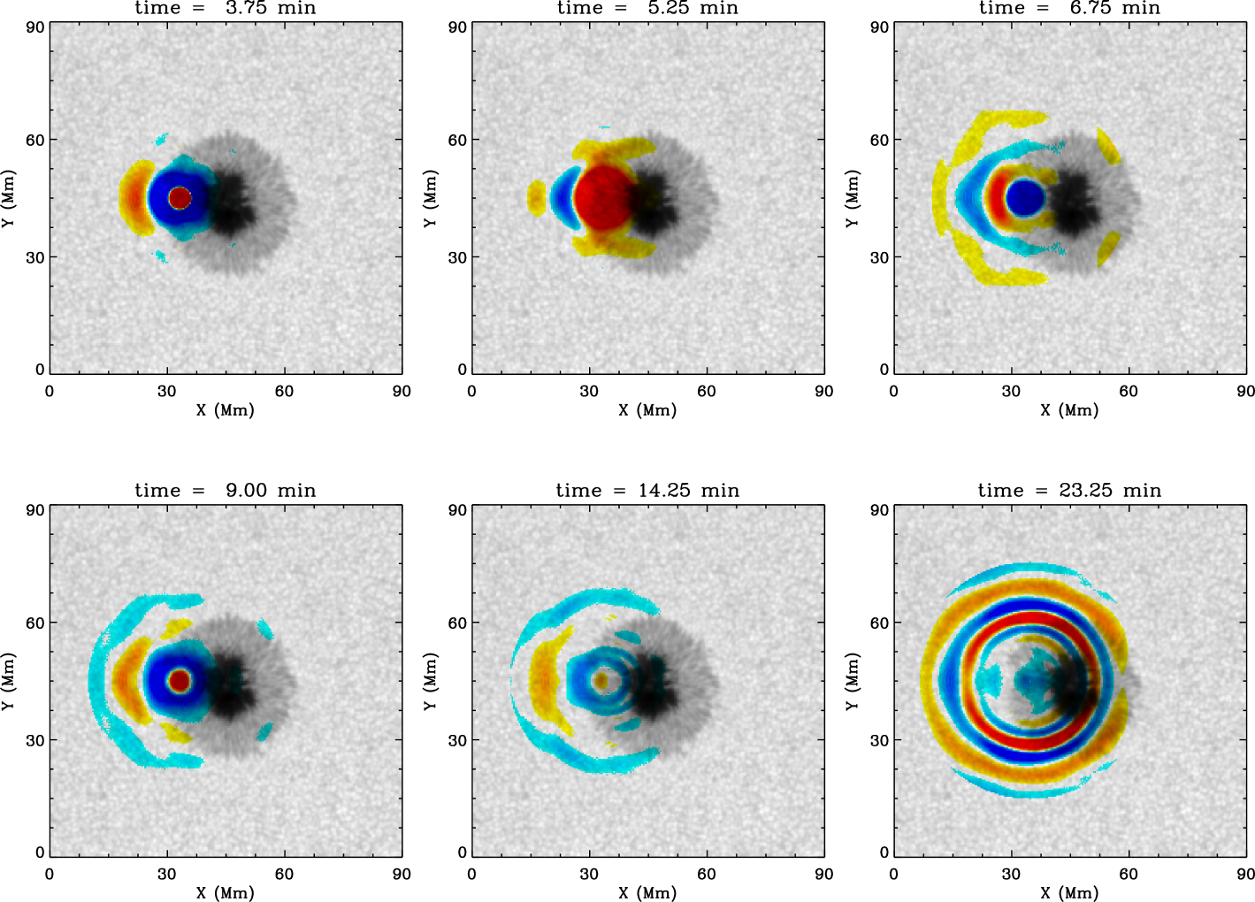
Deep sources of acoustic waves were found in 3D radiative magnetohydrodynamic (MHD) simulations of solar magnetoconvection with a self-organized pore-like magnetic structure (Kitiashvili et al., 2019). The analysis of more than 600 acoustic events inside and outside the simulated pore-like magnetic structure showed that the depths of acoustic events were mostly located below 1 Mm inside the magnetic region. This is substantially deeper than the acoustic wave sources outside the magnetic region. Similarly, to interpret the ripple-like velocity patterns observed in FeI 5435 Å, Cho and Chae (2020) assumed subsurface wave sources and fitted the model to infer a subsurface wave source at a depth of 1-2 Mm.
The work reviewed above confirmed a fast horizontal wave propagation in and around sunspots. This is consistent with an explanation of subsurface wave sources beneath sunspots, although the detailed depths are still uncertain.
It is also important to investigate whether the photospheric waves are connected to the wave phenomena in the upper atmosphere. A time-distance helioseismic analysis method applied to HMI observations together with chromosphere data observed at the Big Bear Observatory and Sacramento Peak Observatory (IRIS instrument) and coronal observations from the SDO Atmospheric Imaging Assembly (AIA) showed that the photospheric waves can channel up from the photosphere through the chromosphere and transition region into the corona along different wave paths with different phase speeds (Zhao et al., 2016). In addition, direct spectroscopic observations by IBIS characterized waves in the sunspot penumbrae with essentially the same dominant periods and propagation speeds, indicating that the chromospheric running penumbral waves are counterparts of the waves observed in the photosphere (Löhner-Böttcher and Bello González, 2015).
10.2 Acoustic Halos
The enhanced power of high-frequency waves surrounding sunspots and plages, known as “acoustic halo”, is an intriguing wave-dynamical phenomenon observed in the solar atmosphere (Khomenko and Collados, 2009). It was first observed in the early 1990s at photospheric and chromospheric heights (Braun et al., 1992; Brown et al., 1992; Toner and Labonte, 1993). This phenomenon is usually observed at frequencies above the photospheric acoustic cut-off of 5.3 mHz, in the range of 5.5 – 7 mHz, over regions of weak to intermediate strength (50 – 250 G) photospheric magnetic field (Hindman and Brown, 1998; Thomas and Stanchfield, 2000; Jain and Haber, 2002; Finsterle et al., 2004; Moretti et al., 2007; Nagashima et al., 2007; Khomenko and Collados, 2009). It was found that the inclination of the magnetic field plays a prominent role in the production of halos (Schunker and Braun, 2011).
A large number of studies centered around modeling acoustic wave – magnetic-field interactions over heights from the photosphere to the chromosphere, with relevance to high-frequency power excess observed around sunspots, have been carried out (see Rijs et al. (2016) and references therein). A central theme of all the above theoretical studies has been the conversion of acoustic wave modes (from below the photosphere) into magnetoacoustic wave modes (the fast and slow waves) at the magnetic canopy defined by the plasma =1 layer.
Utilizing the multi-height capability of HMI and AIA observations, the following properties were found: (i) The halo is present for high-frequency oscillations, beginning at 5.5–6 mHz and up to at least 9–10 mHz. The 6-mHz halo is the strongest in measurements of the Fe I 6173.34 Å Doppler velocity at = 140 km; (ii) The halo magnitude is a clear function of height, with no enhancement in intensity continuum () and in line-wing Doppler velocity ( = 20 km); (iii) In the upper photosphere and chromosphere at the heights sampled by AIA 1600 and 1700 Å wavelength channels (corresponding approximately to = 430 and 360 km, respectively), the halo in the 7–10 mHz range is observed to spread out radially with height, and (iv) about 8 mHz, the spatial extent and structure of the halo change to double halo structure with an inner compact halo surrounded by a diffuse, weak halo region, extending radially many megameters into quiet regions (Howe et al., 2012; Rajaguru et al., 2013; Tripathy et al., 2018, 2020).
In addition, a ring-diagram analysis of active regions observed by the HMI during the first five years showed that the frequency at which the mode amplitude changes from attenuation to amplification is around 4.2 mHz in the quiet nearby regions while it is about 5.1 mHz in the active regions. This effect (which has a very weak dependence on the wave propagation direction) corresponds to the amplitude enhancement found in the acoustic power maps (Rabello-Soares, Bogart, and Scherrer, 2016).
From what has been learned so far, from observations as well as theoretical studies, it is clear that transport and conversion of energy between magneto-acoustic wave modes, which are driven by acoustic waves and convection from below the photosphere and mediated by the structured magnetic field in the overlying atmosphere, provide a plausible approach for identifying the exact mechanism. The instruments HMI and AIA onboard SDO, with photospheric Doppler and vector magnetic field information from the former and the upper photospheric and lower chromospheric UV emissions in the 1700 Å and 1600 Å wavelength channels of the latter, have provided interesting possibilities for such studies. Though none of the proposed theoretical explanations or mechanisms causing the power halos can match all of the observed properties and hence provide an acceptable theory, the mechanism based on MHD fast-mode refraction in the canopy-like structure of strong expanding magnetic field (Rijs et al., 2016) appears to confirm some major observed features (Figure 46).
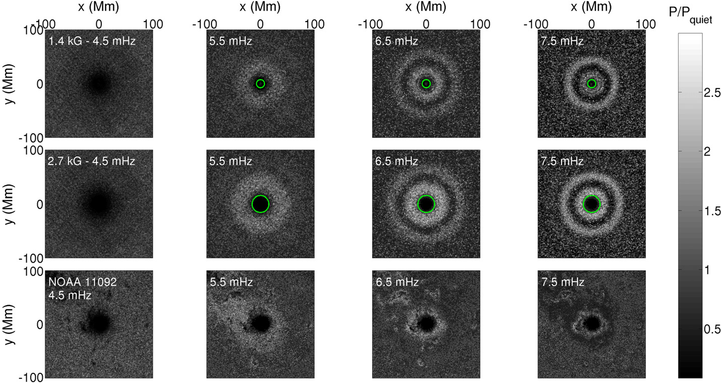
.
10.3 Subsurface Structure and Dynamics of Sunspots
Several helioseismic techniques have been developed to probe the subsurface structure below the sunspots. The most widely used measurement is the phase shifts detected between in and out-bound waves traveling through the active regions and can be obtained through Hankel analysis (Braun, 1995) or time-distance helioseismology (Duvall et al., 1993). The initial attempt to infer the sound speed structure assumed that only the thermal effects are relevant (the direct effect of the magnetic field was neglected) and found a faster wave speed approximately at a depth of 1 Mm below the sunspot (Fan, Braun, and Chou, 1995). Subsequent studies using time-distance helioseismology indicated a two-layer model with reduced wave speed in the top layer and increased wave speed down to 10 Mm below the surface (Kosovichev, Duvall, and Scherrer, 2000). Analysis of HMI Dopplergrams through ring-diagram technique also illustrated a two-layer structure (Gizon et al., 2009). However, a comparison between ring-diagram, time-distance, and Hankel analysis of the sunspot associated with NOAA AR 9787 showed substantial quantitative differences (Gizon et al., 2009, 2010; Kosovichev et al., 2011) and it was suggested that the structure of this particular sunspot is probably associated with a shallow, positive wave-speed perturbation instead of the standard two-layer model (Moradi et al., 2010). Additionally, one cannot rule out the possibility that helioseismic inversions are contaminated by surface effects produced by a strong magnetic field (Couvidat and Rajaguru, 2007).
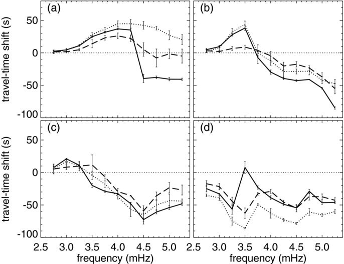
With the availability of faster high-end computational facilities that led to the generation of more realistic artificial data through numerical modeling and its analysis through various helioseismic techniques, we now have a better understanding of the issues associated with wave propagation in strongly magnetized regions. For example, Braun et al. (2012) compared travel-time shifts measured from a realistic magnetoconvective sunspot simulation and two sunspots observed by HMI. Figure 47 shows the averages of the mean travel-time shifts over the umbra of the sunspot measured by helioseismic holography. The study found remarkable agreement below 4.5 mHz but significant differences above it. The most striking difference is seen in the center of the sunspots; the travel-time shifts of the real sunspots are found to be positive, while the corresponding shifts in the simulated spots are negative. Since the hare and hound tests of simulated data considering only sound speed perturbation had shown remarkable agreement between the simulated sunspot and measured shifts (Birch et al., 2011), it is conjectured that the anomaly in the travel-time shifts is caused by the inclusion of the magnetic field. Later studies focused on understanding the interaction of waves with the magnetic field by analyzing data from simulated sunspots. Felipe et al. (2016) investigated travel time shifts arising from magnetic and thermal effects and concluded that for certain combinations of phase speeds and frequencies, the travel time shifts could be explained through the thermal effects alone. These authors later studied the dependence of the travel time on magnetic field strength and Wilson depression (Felipe, Braun, and Birch, 2017) and found that shifts corresponding to frequencies above 3.5 mHz are insensitive to the magnetic field strength (also see Moradi et al., 2015).
10.4 Flows in and around Active Regions
Apart from strong outflows close to sunspots, active regions exhibit much larger inflows around them in the near-surface layers. These flows first detected by the ring-diagram technique typically have amplitudes of 20 – 30 and occur up to a depth of 10 – 14 Mm below the photosphere and extent up to ( Mm) around active regions (Haber et al., 2001; Gizon, 2003; Zhao and Kosovichev, 2004). The ring-diagram analysis using HMI data confirmed these results (Rabello-Soares, Bogart, and Scherrer, 2018; Komm, Howe, and Hill, 2020).
Analysis of the HMI time-distance helioseismology data with a resolution of confirmed these inflows around active regions to have a peak amplitude of 40 m s-1 for the strongest active regions and about 20 m s-1 on average, an extent of up to away for the strongest active regions and an extent of about to on average (Kosovichev and Zhao, 2016; Mahajan, Sun, and Zhao, 2023). Helioseismic holography is another technique that has been used to measure inflows around active regions (Braun, 2019, 2024). It is found that the average inflow profiles around active regions using holography are a factor of two smaller than the ones found by time-distance analysis. It is presently unclear where this difference arises from. Evidence of a deep outflow around sunspots has been observed using Hinode (Zhao, Kosovichev, and Sekii, 2010) and HMI (Rabello-Soares, Bogart, and Scherrer, 2018). This is consistent with a large-scale circular flow in a cylindrical shell around sunspots, with a downflow near the sunspot and an upflow farther away, connecting the near-surface inflow to the deep outflow (Gizon, 2003). These active-region flows, thus, contribute to longitudinal averages of zonal and meridional flows and, thus, to the time-varying global-scale flows (Braun, 2019; Getling, Kosovichev, and Zhao, 2021).
Inflows around active regions impact the solar magnetic cycle in several ways: 1) they may enhance magnetic flux cancellation within active regions as shown by surface flux transport models with inflows (Cameron and Schüssler, 2012; Nagy, Lemerle, and Charbonneau, 2020) 2) they may play a role in perturbing the differential rotation of the Sun and hence contribute to the torsional oscillation pattern (Section 9.2.1) 3) they play a dominant role in the modulation of the near-surface meridional flow (Section 9.2.3) and 4) inflows around active regions combined with hemispheric asymmetry in activity can cause cross-equator flows (Komm, 2022a).
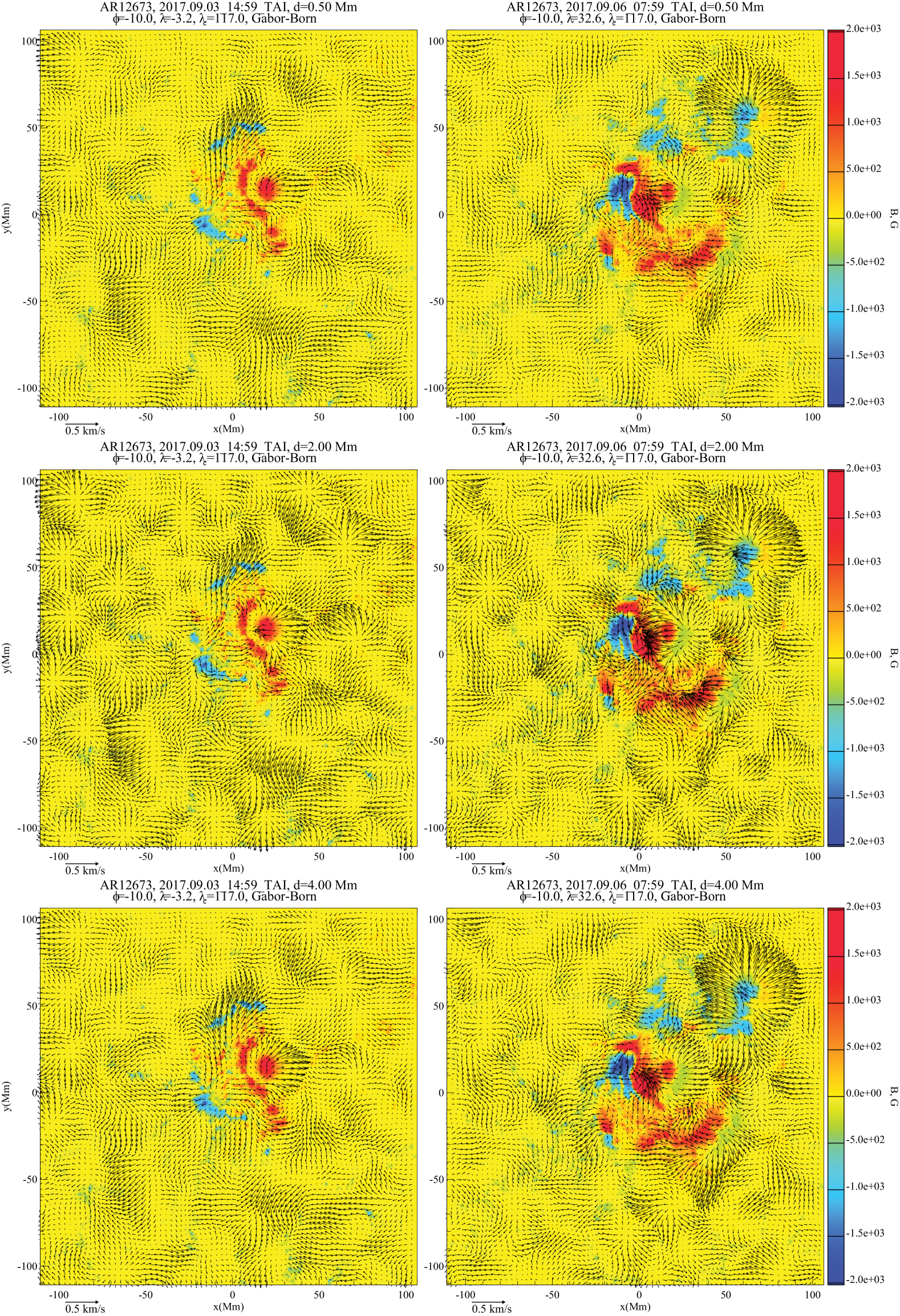
A study of subsurface flows in the emerging active region NOAA 11158 by the ring-diagram technique revealed divergent flows, the magnitude of which decreased around the time of major flares, suggesting that the flow kinetic energy contributed to the energy released by flares (Jain, Tripathy, and Hill, 2015). The subsurface dynamics of emerging active regions inferred from the time-distance helioseismology with higher spatial and temporal resolutions showed that the divergent flow pattern observed at the initial emergence stage changes to predominantly converging flows during the formations of sunspots and flaring activity in the top 4 Mm deep layer while the flows remain diverging in the deeper layers (Kosovichev and Rozelot, 2018; Kosovichev and Sadykov, 2024). Figure 48 illustrates the flow patterns in the active region NOAA AR 12673 during the emergence and before a major X9.3 solar flare.
These studies also indicated a statistically significant correlation between the subsurface flow characteristics and the flare index of active regions. However, a comprehensive study of the complex relationship between subsurface flows, the evolution of active regions, and their magnetic activity has yet to be performed.
Some attempts are also made to explore the flow characteristics in active regions with peculiar magnetic configurations, e.g., anti-Hale and anti-Joy active regions. Authors reported the anti-clockwise or clockwise flows surrounding the anti-Joy active regions depending on their locations in the Northern or Southern hemispheres, respectively (e.g., González Hernández et al., 2013; Jain and Tripathy, 2024; Kosovichev and Sadykov, 2024).
11 Helioseismic Mapping of the Solar Far-Side Active Regions
Active regions observed by HMI on the near side of the Sun are very important for monitoring solar activity and eruptions, and many numerical models using these observations have greatly advanced our understanding of solar eruptions in the last decades. However, many space-weather prediction models, particularly those dealing with solar wind, coronal holes, and global-scale magnetic properties, need far-side information of active regions for more accurate modeling (Arge et al., 2013). Some modelers rely on synoptic maps obtained from magnetograms of the visible surface of the Sun, while others estimate the far-side magnetic field through flux-transport models (e.g., Schrijver and De Rosa, 2003; Upton and Hathaway, 2014b). However, new active regions (ARs) may emerge and rapidly evolve on the far side of the Sun. These ARs cannot be modeled by the flux-transport models, causing inaccuracies in the far-side magnetic field data currently used by the global coronal and solar wind models. Local helioseismology has provided the capability of mapping ARs on the far side of the Sun, which was initially developed for the analysis of the SoHO/MDI data.
11.1 Detection of Far-Side Active Regions Using Helioseismic Holography
While the Sun’s far side is not directly visible in electromagnetic waves from Earth, it is essentially transparent to acoustic waves. This property was employed in the helioseismic holography method, in which the phase shifts are caused by the scattering of waves from the thermal and magnetic perturbations associated with active regions on the far side (Lindsey and Braun, 2000b; Braun and Lindsey, 2001; Lindsey and Braun, 2017). This technique allowed us to map large active regions on the Sun’s far side. The far-side images are routinely obtained twice a day and available online in near-real time 151515jsoc.stanford.edu/data/farside/.
With the availability of STEREO’s far-side EUV images, it became possible to systematically compared the STEREO/EUVI 304 Å images, in which ARs exhibit enhanced emission with the helioseismic holography far-side images made from observations of both GONG and HMI (Liewer et al., 2012, 2014; Liewer, Qiu, and Lindsey, 2017). It was found that 95% of the far-side ARs detected by the holography method correspond to an observed EUV brightening area, but only about 50% of EUV brightening areas correspond to the holography-detected ARs. This gives us a sense of the reliability and limitations of the helioseismic holography far-side imaging method.
Various authors have also tried to improve the detection of active regions in the holographic far-side images. In particular, the far-side ARs were identified with higher sensitivity and better accuracy by applying a machine-learning method (Felipe and Asensio Ramos, 2019; Broock, Asensio Ramos, and Felipe, 2022). The quality of the individual AR imaging on the far side was improved by defining the ingression and egression wavefields in terms of a Green’s function and using an accurate forward solver (Yang, Gizon, and Barucq, 2023). A comparison of ARs observed by the SO/PHI near the far-side limb area found reasonable agreement (Yang et al., 2023).
11.2 Detection of Far-Side Active Regions Using Time-Distance Helioseismology
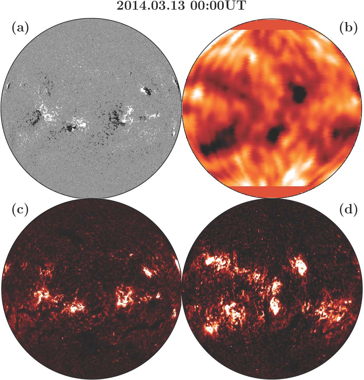
Time-distance helioseismology also demonstrated the capability to image the far-side active regions with a deep-focusing measurements scheme with the acoustic ray focus point on the far side of the Sun (a 4-skip scheme) (Duvall and Kosovichev, 2001). This technique was improved by combining this scheme with 3-5-skip waves (Zhao, 2007; Ilonidis, Zhao, and Hartlep, 2009) and applying numerical simulations that helped to identify and remove spurious signals in the far-side images (Hartlep et al., 2008). The HMI data allowed to include the 6- and 8-skip waves (Zhao et al., 2019), which increased the reliability and accuracy of the far-side imaging (Figure 49). The routine production of the far-side images is available in the near-real time161616jsoc.stanford.edu/data/timed/.
The helioseismic images of the solar far side can also be used to study the solar-cycle properties of the Sun. The far-side images obtained by the holography technique from the SOHO/MDI data showed that the mean helioseismic phase shifts associated with far-side ARs varied substantially with the phase of the Solar Cycle 23 (González Hernández, Scherrer, and Hill, 2009). These variations were attributed to the Sun’s seismic radius change with solar cycles. However, using 11 years (a full solar cycle) of HMI time-distance far-side image data, Zhao, Jiang, and Chen (2021) concluded that the mean phase shifts (or travel-time shifts) in such images are likely due to a collective effect of surface reflections of the helioseismic waves that unavoidably interact with the surface magnetic fields.
11.3 The Space-Weather Connection
The far-side images play an important role in space-weather prediction because they use up to ten days of warning of new large active regions appearing on the Earth’s side (Jain et al., 2023). For example, Figure 50 shows the helioseismic signature of the strong active-region complex consisting of ARs 12785 and 12786, which crossed the Sun’s south-eastern limb on 2020-11-23.
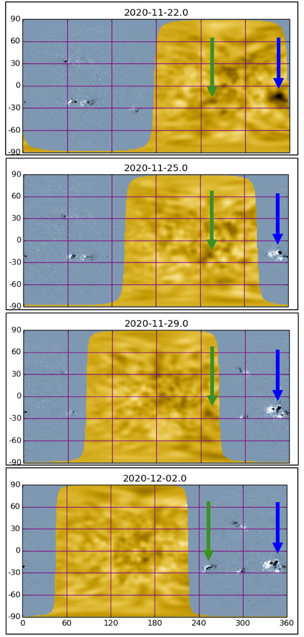
Another active region, AR 12781, indicated by the green arrow, approached the south-eastern solar limb five days later and produced a series of flares.
11.4 Converting Far-Side Helioseismic Images into Magnetic-Flux Maps
As pointed out earlier, the far-side magnetic fields are important to global-scale modeling efforts, but the helioseismic far-side images are unsigned measurements of acoustic phase shifts. Converting acoustic signals into magnetic signals is one crucial step toward fully mapping the far-side magnetic fields. Previous authors have established that the EUV 304 Å images can be used as a proxy for the magnetic field (e.g., Ugarte-Urra et al., 2015; Kim et al., 2019), and the acoustic phase shifts can be used as another proxy for the magnetic field (González Hernández, Hill, and Lindsey, 2007). Figure 49 shows well the relations among these properties.
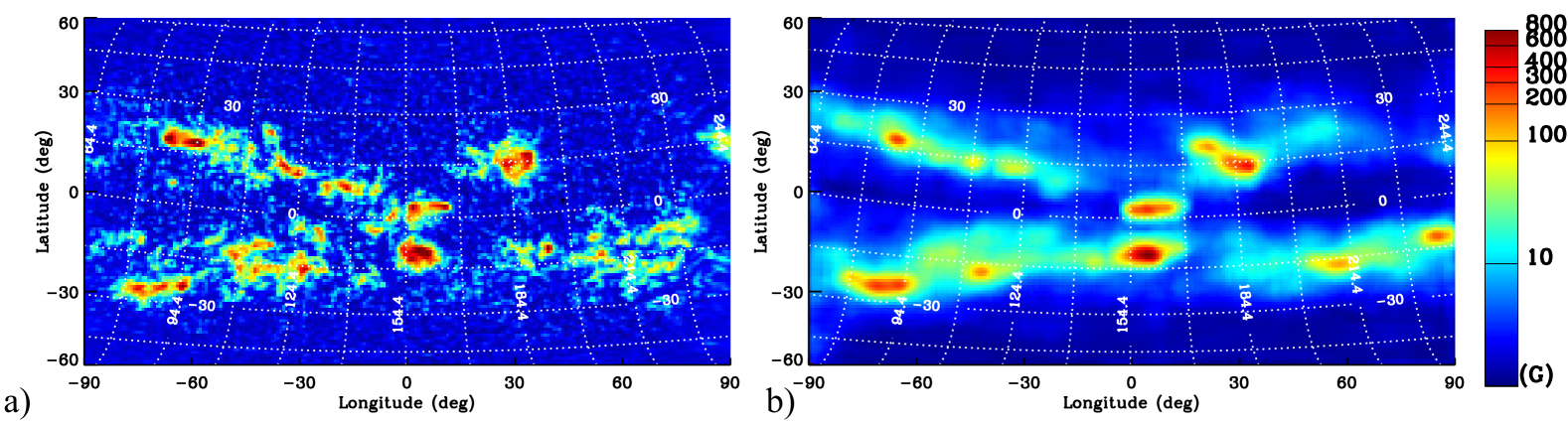
Two machine-learning techniques were used to convert the time-distance far-side images combined with the far-side 304 Å images from STEREO into far-side magnetic-flux maps (Chen et al., 2022). Figure 51 shows an example of magnetic-flux maps generated by this technique. Despite the success of these machine-generated far-side magnetic-flux maps, their usefulness is still limited because this method is unable to produce the polarities of the magnetic field.
12 Early Detection of Emerging Magnetic Flux
Detection of emerging active regions (ARs) before they become visible on the solar surface is tightly linked to understanding the coupling of the activity of the Sun on the global and local scales. This understanding is crucial for advancing our capabilities to predict solar activity and its impact on Earth’s environment. In particular, theoretical and numerical efforts suggest that ARs form from magnetic flux ropes generated in the solar interior (e.g., Parker, 1994; Fan, 2021) that emerge on the solar surface. However, understanding how and where the magnetic flux is organized in highly magnetized magnetic field bundles, how they evolve during emergence through the convective layers, and how surface and atmospheric layers respond and manifest the upcoming emergence continue to require a detailed theoretical investigation and detailed analysis of observations.
Whole-disk observations with HMI over the solar cycle enable the investigation of emerging ARs from the deep interiors to the photosphere. Since the evolution of subsurface dynamics cannot be observed directly, it can be inferred from photospheric disturbances that are sensitive to structural and dynamical changes through all layers of the convection zone using helioseismic and other methods. In this section, we review advances in the detection of emerging ARs and the analysis of surface and subsurface dynamics to identify precursors of the emergence with different helioseismic techniques (Section 12.1) and alternative approaches, including tracking of the photospheric flows and machine-learning approaches (Section 12.2), as well discussion of still-open questions and expectations for future developments (Section 12.3).
12.1 Diagnostics of Emerging Magnetic Flux from Helioseismic Analyses of HMI Data
The emergence of ARs is usually associated with a significant increase of magnetic flux in the photosphere, accompanied by strong diverging flows, a rapid decrease of continuum intensity, and substantial restructuring in the solar atmosphere (for a review of the topic see van Driel-Gesztelyi and Green, 2015). However, before AR emergence, there are generally no obvious signatures of upcoming flux due to slow changes in local thermodynamic properties in the solar interior.
Most previous helioseismic investigations by the time-distance technique (Section 3.2) (e.g. Ilonidis, 2012; Kholikov, 2013; Birch et al., 2013) have found negative travel time shifts (typically corresponding to an increase in local wave speed), and the regularity with which they have been detected suggests that there is potential for them to be used as an indicator of the magnetic field emergence with the following formation of ARs. Early evidence of this can be found in an increase in the sound speed perturbations inferred by a time-distance inversion technique in the uppermost 18 Mm of the convection zone before the emergence of an AR (Kosovichev, Duvall, and Scherrer, 2000). Tracking the evolution of the acoustic wave speed perturbation allowed the authors to obtain one of the earliest observational constraints on flux rise speed, estimating that the speed of emergence is about 1.3 km s-1.
The capability to detect a signal in the deep convection zone hours before the AR emergence was demonstrated by applying a deep-focus time-distance scheme (Ilonidis, Zhao, and Kosovichev, 2011) and a similar approach (Kholikov, 2013) to the MDI and Global Oscillation Network Group (GONG) data. The follow-up analysis of AR 11158 pre-emergence helioseismic signal from SDO/HMI observations (Ilonidis, 2012; Ilonidis, Zhao, and Hartlep, 2013) showed an increase in the local wave speed consistent with the earlier investigations (Kosovichev, Duvall, and Scherrer, 2000; Ilonidis, Zhao, and Kosovichev, 2011).
Subsequent work focused on improving the signal-to-noise ratio by applying an averaging procedure and varying the signal threshold (Stefan, Kosovichev, and Stejko, 2021). Testing of this new approach was performed on two simulations with imposed sound speed variations showed that the method was most sensitive to deeper perturbations (50 Mm to 60 Mm beneath the simulated photosphere). This approach enabled the detection of a robust signal from several ARs up to 26 hours before the emergence. Figure 52 shows an example of the successful detection of AR 11158 at least 20 hours before it emerges. Panel (a) traces the evolution of the unsigned surface magnetic flux (red) and the perturbation index (black). The perturbation index is a measure that integrates travel-time perturbations beyond a given threshold to reduce the contribution from the background noise (Ilonidis, Zhao, and Kosovichev, 2011). Figure 52a displays a gradually increasing perturbation index that peaks most sharply around 8-10 hours prior to the time of emergence (the dashed red line). Figures 52b and c show the corresponding travel-time map at the peak and the configuration of the surface magnetic field at the end of emergence, respectively. Later application of this methodology to 46 ARs showed the capability to detect a signal of the emerging flux at least 24 hours before emergence at the photosphere for 28 ARs (Stefan and Kosovichev, 2023). In particular, a correlation was found between the emergence rate and amplitude in travel time shift variations. Therefore, faster emergence (that typically corresponds to larger magnetic flux due to stronger buoyancy force) allows earlier detection.
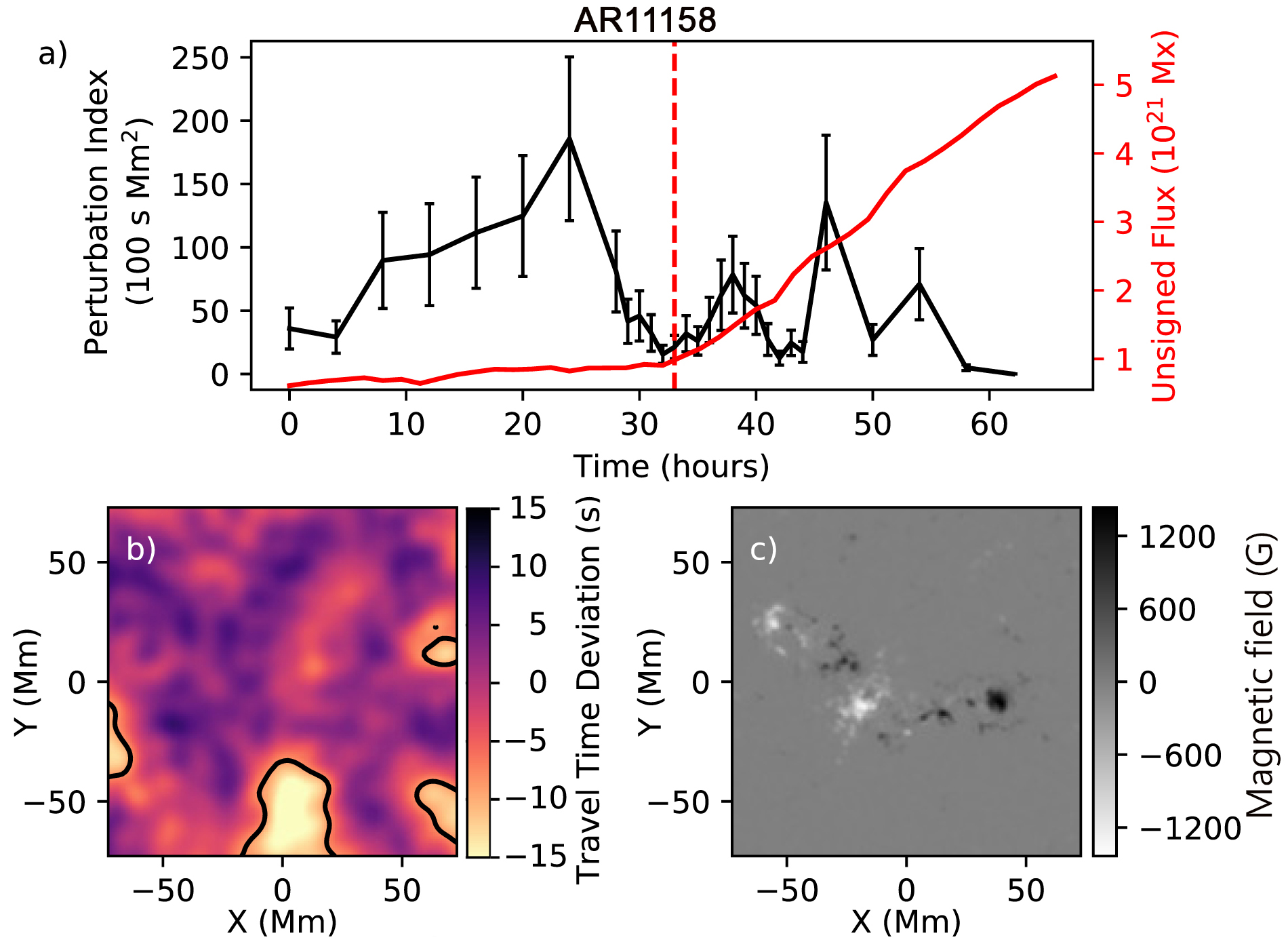
12.2 Emerging Flux Inferences Based on Tracking of Surface Dynamics
While detection of emerging magnetic flux via helioseismic may be the most direct method for making forecasts of AR emergence, there have also been significant efforts focused on forecasting the emergence of ARs directly from HMI observations. Such works use HMI’s observations of the photosphere and search for subtle changes in the surface velocity, brightness, and magnetic field.
12.2.1 Flow Tracking Techniques
One of the more robust photospheric signatures is the horizontal diverging flow (HDF) field which forms on the surface just before the flux concentration emerges on the photosphere. Simulations show that HDF results from a “squeezing” of plasma above the rising flux concentration and below the stably stratified atmosphere (Cheung et al., 2010; Toriumi and Yokoyama, 2013), and that the magnitude of this diverging flow field is directly related to the flux rise speed (Birch, Braun, and Fan, 2010; Birch et al., 2016).
Direct measurement of these HDF flows is challenging; however, since they are oriented perpendicular to the photosphere and HMI can measure only line-of-sight (LOS) velocity. Two strategies have been developed to overcome this limitation. First, focusing on observations close to either the West or East solar limb means that the LOS velocity incorporates a greater amount of the horizontal component, and the horizontal diverging flows can be discerned from the background convection based on overall spatial extent (larger than convective cells) and configuration (positive and negative Doppler velocities, generally aligned with magnetic dipole axis). An examination of HMI Dopplergrams centered around the eventual location of AR 11081 (25 degrees away from the central longitude) found an HDF that develops around 100 minutes before clear flux emergence (Toriumi, Hayashi, and Yokoyama, 2012). In this case, it was impossible in this case to distinguish between the radial and horizontal components of the flow from the LOS velocity, but tracking the outflow pattern in Doppler images revealed that the positive and negative centroids of these flows drifted apart at speeds between 0.6 and 1.2 km s-1. Further examination of other ARs using a similar strategy also found HDFs in around a third (Rees-Crockford, Nelson, and Mathioudakis, 2022) to around half (Toriumi, Hayashi, and Yokoyama, 2014) of the AR samples.
An alternative approach is to perform feature tracking based on either HMI Dopplergrams, magnetograms, or intensitygrams that allow for the horizontal velocity to be extracted by differentiating the feature position with respect to time. The advantage of this approach is that HDFs can be measured anywhere on the solar disk, potentially leading to a more general robust forecasting tool. One particular application of this methodology is the Balltracking algorithm (Potts, Barrett, and Diver, 2004; Attie and Innes, 2015). This method treats the magnitude of the continuum intensity measured by HMI as “height”, down which simulated balls are allowed to roll, mimicking how a physical object would be pushed around by granular flows. The Balltracking algorithm was applied to the intensitygrams to investigate the evolution of horizontal flows around AR 12673 to search for pre-emergence signatures of the secondary flux, which emerges close to the central, mature sunspot (Attie et al., 2018). The authors find that the radius of the moat flow is perturbed up to 35% at four different locations, occurring up to 12 hours before the secondary flux emerges. Most notably, the deviation of the moat flow occurs directly over the flux concentration, “pointing” in the direction of new flux. Thus, this method has the potential to identify secondary flux emergence, which is difficult to perform using helioseismic methods due to the complicated interaction between p-modes and existing magnetic flux concentrations.
12.2.2 Machine-Learning Applications
The prediction of emerging flux using more modern data processing techniques, such as Machine Learning (ML), is still a rather unexplored area of study. Currently, machine learning studies are primarily concentrated on properties and dynamics of already formed active regions, such as automatic identification of active regions on the solar surface (e.g., Quan et al., 2021; Madhan and Sudhakar, 2023; Mourato, Faria, and Ventura, 2024). A recently developed machine learning approach for the detection of emerging active regions (Kasapis et al., 2024a) is based on previous demonstrations of a correlation between variations in acoustic power and the presence of strong subsurface magnetic fields or upcoming flux (Hartlep et al., 2011). Utilizing the trained Long Short-Term Memory (LSTM; Sherstinsky, 2020) – which is most suitable for the analysis of time-series of HMI/SDO observables – a series of physics-informed ML models have been developed and tested. During the training phase on 40 ARs, the LSTM models analyze correlations between acoustic power in four frequency ranges and the unsigned magnetic flux and corresponding continuum intensity variations that allowed to predict a decrease of the continuum intensity associated with an AR emergence (Kasapis et al., 2024b). To evaluate the performance of the developed ML models, the time criterion of AR emergence was defined as the time that follows a sustained (for more than 3 hours) decrease in continuum intensity with a rate of 0.01.
The developed model can predict continuum intensity in both subareas (tiles) where the emergence of an active region is expected (e.g., Tile 40 and 41 in Figure 53) and tiles where photospheric dynamics remain quiet (Tile 38). Magnetic flux can occupy more than one tile or be transported from one tile to another during the emergence process, and the model can capture these changes. For instance, Tile 40 shows a delay in the predicted and observed continuum intensity decrease compared to Tile 41. In general, the LSTM model predictions are in reasonable agreement with observations of the changing continuum intensity before and during AR emergence. However, as emerging flux forms an AR, these deviations to the continuum intensity can be significant due to the complexity of the magnetic field structure, which is not considered during the model training. Testing of the LSTM model demonstrated the capability to predict its emergence for the following active regions and time scales: 5 hours in advance for AR 13179, 10 hours for AR 11726, and 29 hours for AR 13165. This new capability is an initial attempt to create a path towards efficient processing of observations and a future application of this capability for the operational forecast of AR emergence.
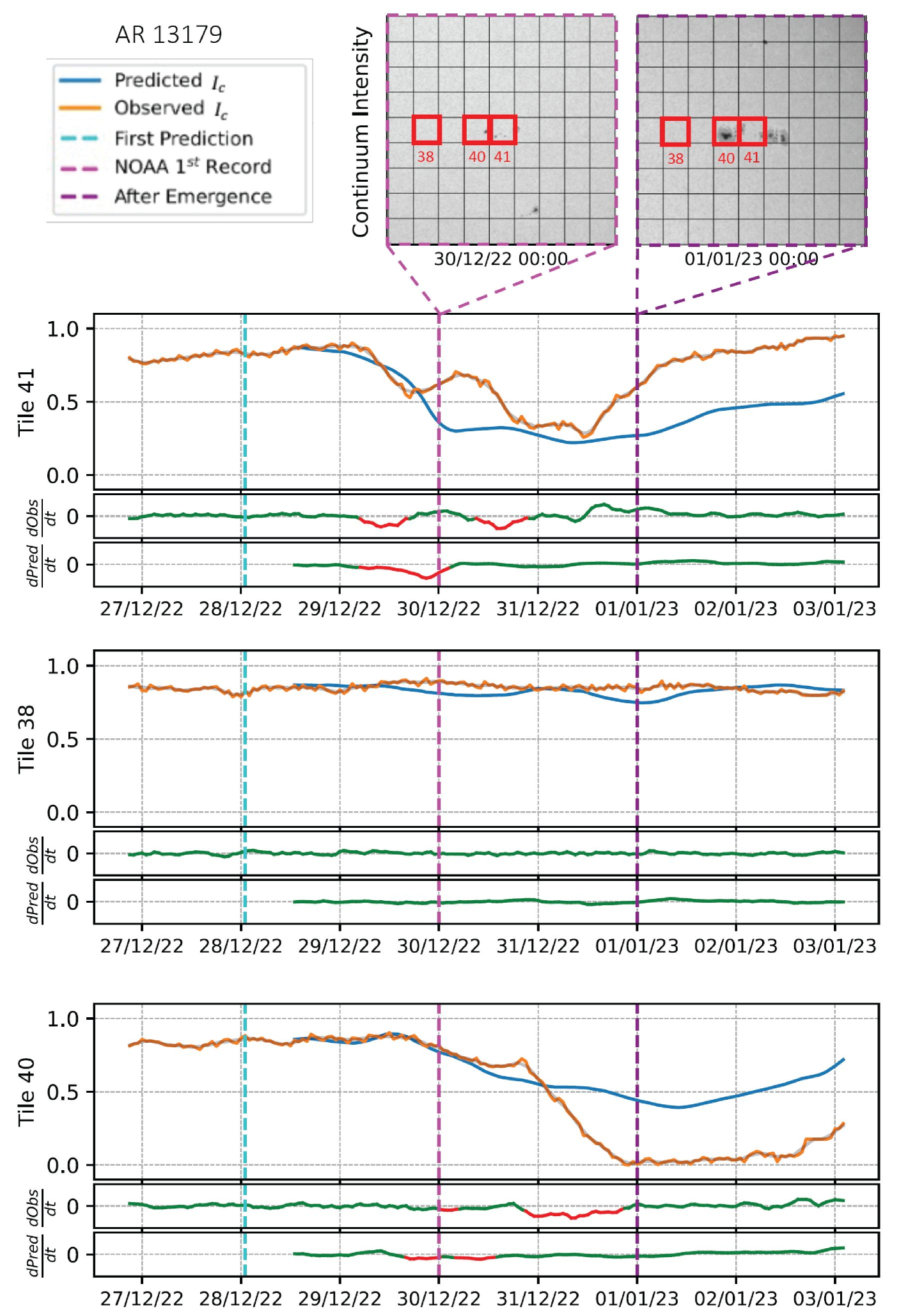
In contrast, a machine learning method applied to detect signatures in super-granular scale flow patterns associated with magnetic flux emergence in the quiet Sun found no systematic features (Mani et al., 2024). It was concluded that emergence was neither systematically influenced by nor affected supergranular-scale flows in their vicinity.
12.3 Open Questions
Work in the pre-HMI era laid a strong foundation for the forecasting of AR emergence, and many successful efforts have used HMI data to build upon these foundations. Still, many significant open questions remain regarding the detectability and physical origins of emerging magnetic flux. Perhaps the most important open questions are those regarding the mechanism by which the helioseismic precursors of AR emergence are generated. For example, several investigations have found mean phase travel-time perturbations that precede the emergence of ARs that are consistent with increases in the local wave speed. Yet, the direct contribution of the magnetic field to wave speed in the deeper ( Mm) convection zone is expected to be completely undetectable, producing travel-time variations on the order of to s (Braun, 2012). Therefore, the mechanism that generates the observed travel-time perturbations is still unclear.
Despite this, there has been some success in measuring horizontal magnetic fields in the shallow convection zone (down to 15 Mm) of existing, stable sunspots (Stefan and Kosovichev, 2022a). Since the speed of magnetoacoustic wave propagation depends on the direction of wave propagation relative to the magnetic field, measuring the travel time of acoustic waves in several different directions allows for the magnetic field’s contribution to be isolated. This methodology has been applied to several simulations and, most notably, several ARs observed by HMI. Figure 54 shows the results of applying this methodology to HMI Dopplergrams centered on AR 12218, where changes to the configuration of the magnetic field over depth can be tracked. An inversion for the magnetic field has not yet been attempted, so the magnitude of the horizontal magnetic field is quantified in terms of a travel-time shift; however, the direction of the horizontal field can be directly measured from the travel times. However, how this methodology can be applied to the forecasting of AR emergence is unclear since it requires relatively long integration times (24 hours). Additionally, the uncertainties for this methodology are significant for weak magnetic fields; this sets a minimum detection threshold on the order of several hundred gauss.
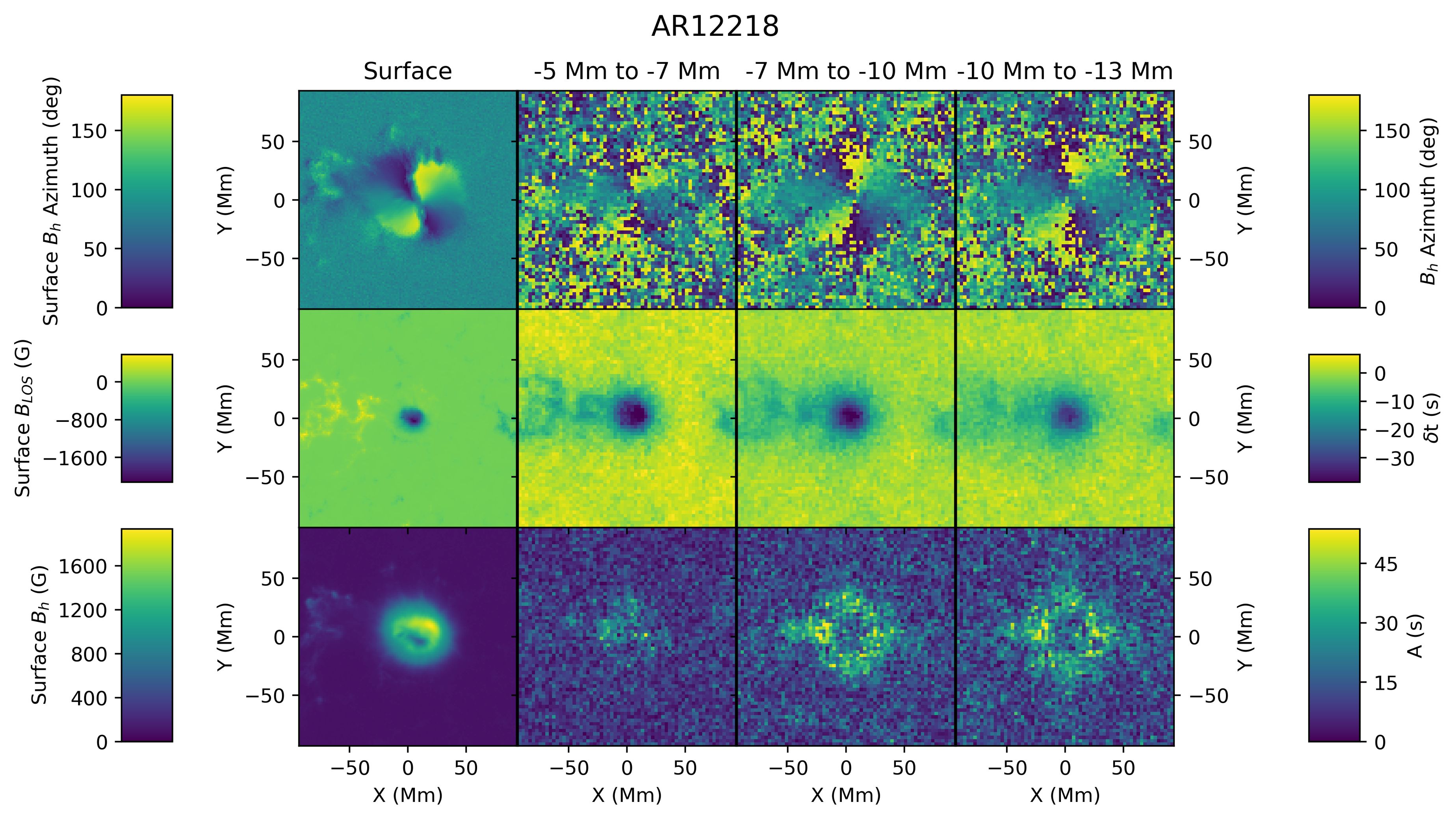
Additionally, purely acoustic waves (p-modes) are not the only mode to have been investigated as a probe of interior magnetic fields. In particular, changes to the power of the surface gravity mode (or f-mode) have been identified as a potential precursor to AR emergence. Analyses of idealized MHD simulations have found that the f-mode tends to “fan out” in the Fourier space in the presence of horizontally non-uniform magnetic fields, where the f-mode power at any particular wavenumber is spread over a broader range of frequency space than in the unperturbed state (Singh, Brandenburg, and Rheinhardt, 2014). The exact mechanism of the f-mode fanning and the associated increase in the f-mode power is not well understood, but a scattering of p-modes by the magnetic flux and subsequent leaking into the f-mode has been suggested as a possible explanation.
Furthermore, investigations of changes to the f-mode on the Sun have produced mixed results. Early work examined how the f-mode power derived from HMI Dopplergrams in six pre-emergence regions changes with respect to quiet regions at the opposite latitude and identical longitude. Ideally, such a comparison will control for variations in the f-mode power related to the distance from the disk center. It was found that all six isolated pre-emergence regions show an increase in the f-mode power at high wavenumbers (corresponding to =1200 – 2000) one to two days before emergence (Singh, Raichur, and Brandenburg, 2016), and in most cases, this increase in the f-mode power exceeds that observed in the opposite hemisphere. The results of this particular investigation were called into question by later work, however, where an improvement in the procedure used to calibrate the f-mode power against longitudinal variations reduced the changes in f-mode power in ARs 11105 and 11130 to within the quiet Sun uncertainty range (Korpi-Lagg et al., 2022).
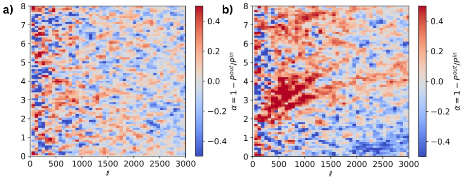
A re-analysis of the same ARs by using a Fourier-Hankel decomposition (Waidele et al., 2023) showed that there is indeed a statistically significant increase in the f-mode power in ARs 11158, 11768, 11130, and 11072 which is consistent with the previous results. However, the measurement of the absorption coefficient showed no absorption or emission during f-mode power enhancement (Figure 55, Waidele et al., 2023). This result questioned the mechanism of p-mode to f-mode conversion via scattering, which was hypothesized in earlier work.
The lack of a precise description of changes in the f-mode power and subsurface magnetic field raises a broader question: what is the relationship between wave propagation and magnetic fields? Many efforts have investigated various aspects of this relationship, for example, disentangling the magnetic effects on wave travel times from thermal effects (Felipe et al., 2016), conversion of acoustic waves to MHD waves (Khomenko and Collados, 2006), and the influence of surface magnetic fields on helioseismic measurements (Lindsey and Braun, 2005). A comprehensive understanding of the interaction between magnetic fields and acoustic waves remains unclear, though, especially for complicated configurations of the magnetic field such as those found in solar ARs.
12.4 Summary
To conclude, there have been many investigations using HMI data to search for pre-emergence signatures of ARs. Time-distance helioseismology has revealed the presence of mean phase travel time deviations which occur before the AR emergence, in some cases more than 24 hours before the flux concentration reaches the surface. The mechanism that generates these deviations remains to be determined, though, as the direct effect of the magnetic field is expected to be small. Other, more straightforward methods have also found precursors of active region emergence, such as measuring surface horizontal diverging flows (HDFs) that develop within 1-2 hours before emergence. Enhancement to the f-mode power has also been suggested as a precursor, though the methodology required to measure these changes is highly sensitive to calibration and normalization procedures and is still somewhat controversial. Finally, the recent work using a type of neural network has been able to predict changes to the continuum intensity that is associated with surface magnetic flux.
13 Sunquakes
13.1 Introduction
The potential connection between solar flares and acoustic oscillations has been a subject of interest since the early days of helioseismology. Wolff (1972) initially proposed that flares could stimulate high-order modes of solar whole-body oscillations. While some studies reported changes in p-mode parameters associated with flares (Maurya, Ambastha, and Tripathy, 2009; Maurya, Ambastha, and Chae, 2014), other studies did not find correlations between high-frequency p-modes and flares (e.g. Richardson, Hill, and Stassun, 2012; Kumar et al., 2017). A comprehensive analysis using ring-diagram techniques on MDI and HMI data found no amplification in mode amplitudes due to flaring activity larger than a 10 percent uncertainty (Rabello Soares, Baudin, and Teixeira, 2021). As a result, Wolff’s original suggestion that flares could excite whole-Sun oscillations remains an open question in solar physics.
However, helioseismic observations performed in 1996 by the MDI instrument detected local helioseismic waves excited by a solar flare (Kosovichev and Zharkova, 1998). These waves formed concentric ripples traveling from the flare source, resembling seismic waves during earthquakes. Therefore, this phenomenon was dubbed ‘sunquake’. The primary interests in studying sunquakes are, first, understanding the physical mechanism of flare impacts that cause helioseismic waves of a relatively high amplitude that reaches several hundred m/s, exceeding the amplitude of background solar convection and oscillations, and, second, understanding how these waves interact with magnetic fields and plasma flows in active regions.
Observations of several powerful sunquake events by MDI during Solar Cycle 23 showed that sunquake sources are associated with flare hard X-ray emission, both spatially and temporally. It was also found that the wavefronts are often anisotropic, perhaps due to the wave interaction with flows and magnetic fields and also because of the multiple flare impacts usually distributed along the magnetic field polarity inversion line in active regions. The close association with the hard X-ray sources indicated that the sunquake may be caused by energetic electrons penetrating deep into the solar atmosphere, in accordance with the ‘thick-target’ model of solar flares. However, the radiative hydrodynamic simulations of this model showed that the particle beams do not reach the solar photosphere and thus can heat only the upper and middle chromosphere, causing chromospheric evaporation. It was suggested that sunquake impacts could be caused by shocks traveling downward from the heated area. However, these shocks quickly decay and do not produce the required energy and momentum transfer in the photosphere. Therefore, additional mechanisms have been discussed, such as the Lorentz force associated with coronal mass ejections, proton beams, and correlation with convective downdrafts. One of the difficulties was that the MDI observations with sufficient resolution (2 arcsec/pixel) were performed only two months a year, and, therefore, the statistics of sunquakes were incomplete.
The uninterrupted high-resolution (0.5 arcsec/pixel) observations with the HMI instrument have opened new perspectives for studying sunquakes. It turns out that sunquakes are more common than assumed before and can be initiated by relatively weak flares (in terms of the flare X-ray class), while many strong X-class flares do produce sunquakes. The high temporal cadence of the HMI observations allows us to discover high-frequency acoustic signals of sunquakes. The exact timing of the photospheric impacts relative to the X-ray signals can be measured by using the HMI filtergram data taken every 3.75 seconds. In addition, the links between the sunquake sources, white-light emission kernels, and rapid magnetic field variations are investigated by analyzing the Stokes profiles of the photospheric Fe I 6173 Å line observed by the HMI.
This section overviews the observational results from HMI and theoretical models motivated by the observations.
13.2 Detection Methods
The detection of sunquakes depends on the amplitude of the excited wave relative to the background solar oscillations and convective flows. Because of the impulsive excitation source, the power of the flare-excited waves peaks in the high-frequency range of solar acoustic oscillations, typically above the acoustic cut-off frequency of the solar atmosphere, which is about 5.2 mHz (Alvarado-Gómez et al., 2012a). In this frequency range, the background convection power diminishes. Sunquake waves are most easily detected by applying a high-frequency filter centered at about 5 – 6 mHz, and sometimes even at higher frequencies (Zharkov et al., 2011; Matthews et al., 2015; Lindsey et al., 2020).
The most unambiguous evidence of a sunquake is the visual detection of the expanding ring-shaped ripples from the flare site in the filtered Dopplergram images (e.g., top panels of Figure 56b). The ripples are usually best observed starting about 20 minutes after the impulsive flare impacts observed in the HMI Dopplergrams as a high-velocity signal Figure 56a) and also in the continuum intensity images as white-light flare kernels (Figure 57d-e). Because of the fast and strong variations in the HMI Fe I 6173 Å line profile (Figure 57g), the physical properties of these impacts are difficult to assess (Sadykov et al., 2020; Kosovichev, Sadykov, and Stefan, 2023).
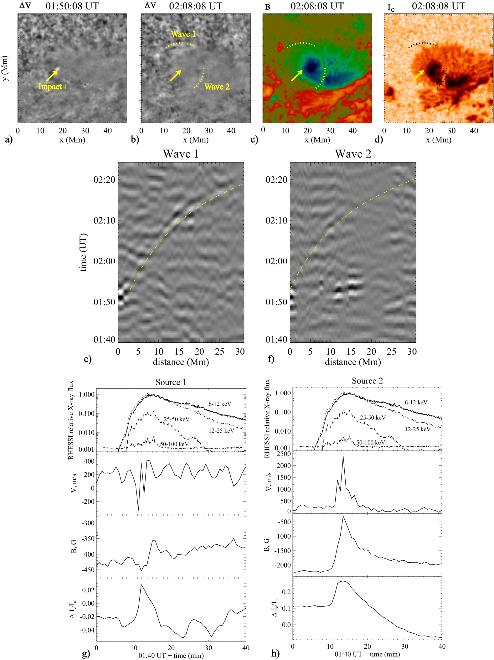
While expanding ripples are visible in some strong sunquakes, they can be challenging to observe in weaker sunquakes obscured by various background oscillations. A more effective method for detecting these sunquake waves is through a time-distance diagram, which involves averaging time sequences along thin annuli or arcs around the flare footpoints and stacking them by distance. This approach enhances the signal-to-noise ratio by averaging along the wavefront of the ripples, making the sunquake waves more visible against the background. As shown in Figures 56(e-f) and 57(c), the propagation of the sunquake wave is clearly visible and aligns well with the theoretical time-distance relationship (yellow-dashed curve).
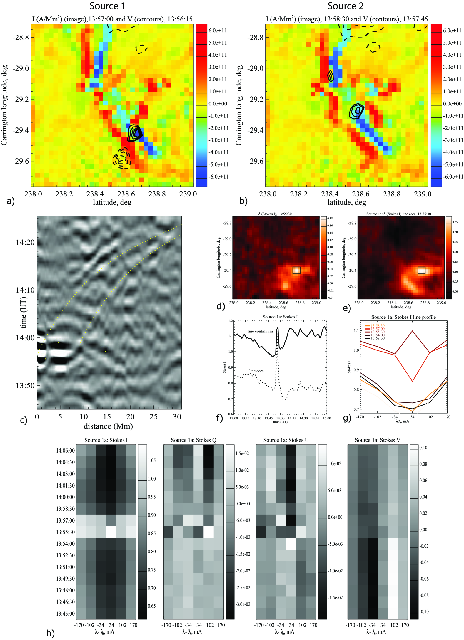
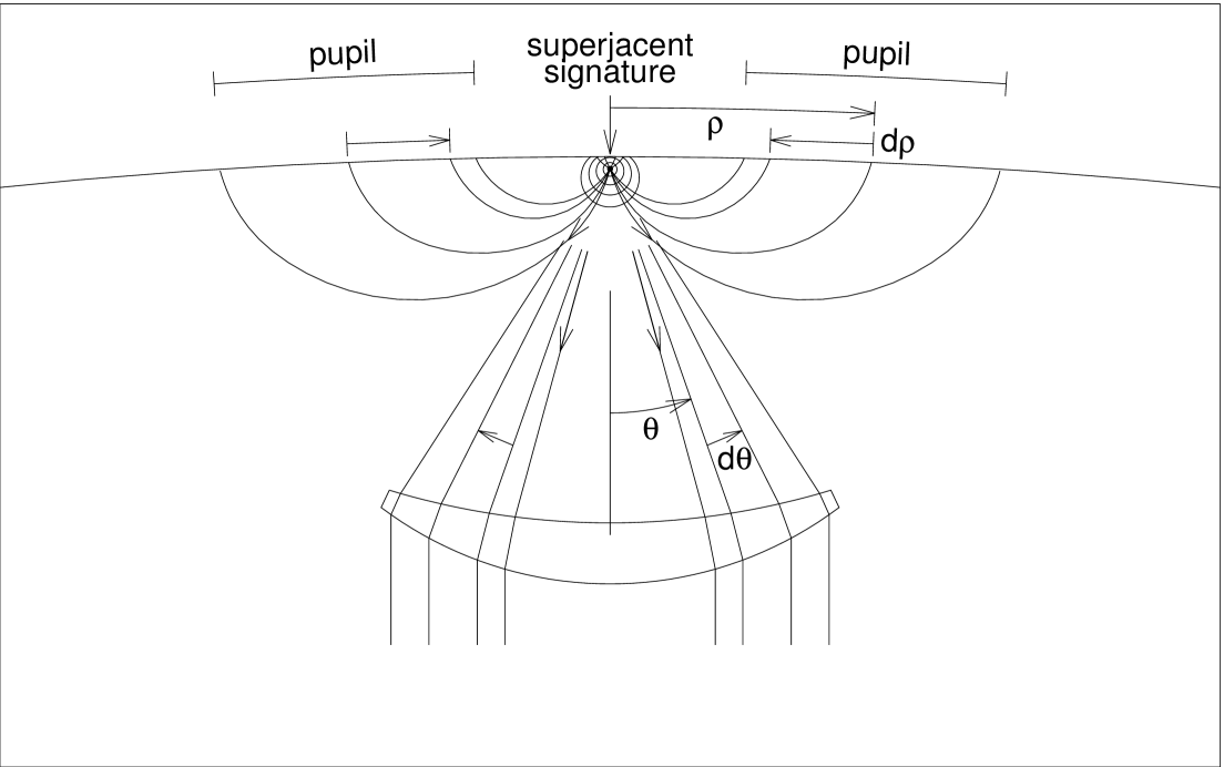
Another detection method is the helioseismic holography method (e.g. Lindsey and Braun, 1997; Donea, Braun, and Lindsey, 1999; Lindsey and Braun, 2000a; Donea and Lindsey, 2005). Helioseismic holography can be thought of as a computational implementation of basic principles of wave optics, running a numerical simulation of the job done in familiar electromagnetic optics by lenses in regressing the wave field to the neighborhood of its source (Figure 58). Among its utilities is mapping the source-power density (hence, just “source density”) of acoustic transients emitted by acoustically active flares. In this capacity, the diagnostic delivers diffraction-limited acoustic images of the acoustic sources it focuses on. Figure 59 shows an example of the diagnostic applied to helioseismic observations of surface ripples emanating outward from the M9.3-class flare of 2011-07-30 in NOAA AR 11261 (Martínez et al., 2020). Both sources, compact to within the acoustic diffraction limit of 10-mHz acoustic waves from the source region, appear on conspicuous boundaries, the left on the boundary separating a sunspot umbra from the adjoining quiet Sun, and the right split along a penumbral magnetic neutral line.
Applied to outgoing surface ripples from a transient acoustic source, the computational task of helioseismic holography is to reverse the acoustic waves in the solar interior, of which the ripples are the surface manifestation, to the neighborhood source location and time, by applying Green’s functions, which describe how waves propagate in the medium. Theoretical Green’s functions, which are noise-free and calculated from a quiet-Sun model, are commonly used in holography studies and generally work well for reconstructing sunquake sources (Chen and Zhao, 2021). This enables a statistical analysis of the temporal relationship between flares and the reconstructed sunquake velocities.
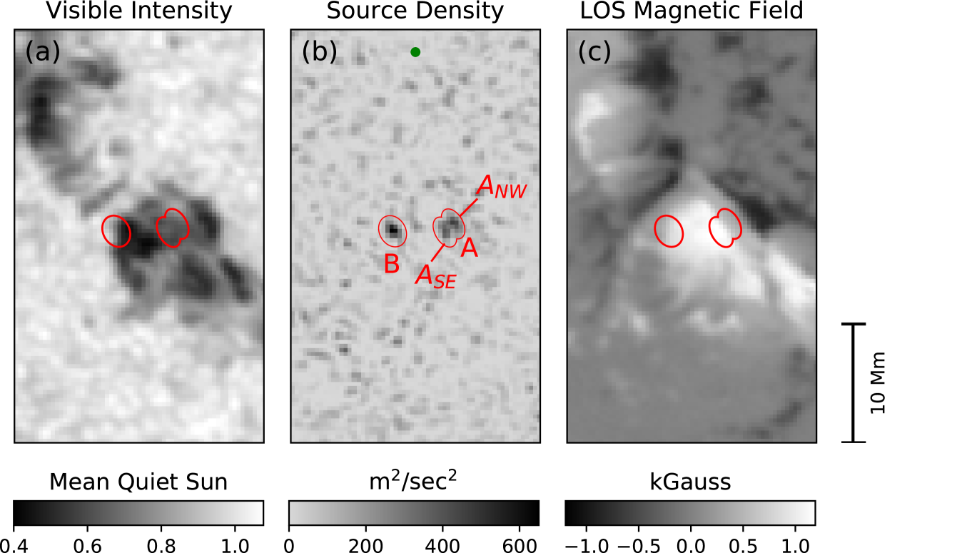
A recent study introduced a novel approach using ML techniques to enhance the detection of sunquakes (Mercea et al., 2023). This method is still in the prototype stage but has demonstrated the potential to identify weak acoustic emissions that may be difficult to detect using conventional methods.
13.3 Theoretical Interpretations and Models
Mechanisms so far considered as contributors to the seismic emissions of flares can be summarized as follows.
Shocks. Flares exhibit strong particle acceleration, as reflected in their hard X-ray and -ray spectra. The high-energy particles producing these radiations can penetrate into the solar atmosphere, resulting in “thick-target” heating of the chromosphere. This heating ejects some of the material up into the corona. The intense heating in the thick target, including the dynamic effects of the ejection, excites downward shock waves that carry some of the flare energy to the photosphere, potentially becoming the source of the seismic emission (e.g. Kostiuk and Pikel’ner, 1975; Kosovichev and Zharkova, 1995; Nagai and Emslie, 1984; Fisher, Canfield, and McClymont, 1985; Allred et al., 2005).
Back warming. Much of the downward radiation from a heated chromosphere (the visible continuum, specifically) should penetrate deeper into the atmosphere and be absorbed (e.g. Hudson, 1972). The resulting photospheric heating, known as “back-warming” (Gordovskyy et al., 2005), if it is sufficiently compact, can generate acoustic transients propagating into the underlying subphotosphere Donea et al. (2006).
Penetrating particles. High-energy protons can penetrate into the low photosphere and heat it directly (Najita and Orrall, 1970; Gordovskyy et al., 2005). This mechanism requires large particle beam intensities at high energies of order 100 MeV for protons. Very energetic particles can indeed penetrate below the photosphere, thus optimally transferring momentum and energy between the corona and interior. However, a seismically active flare (SOL2005-01-15T00:43) without appropriate -ray emission led to the arguments that sunquakes may not be caused by high-energy protons (Moradi et al., 2007; Kosovichev, 2007). Recent radiative hydrodynamics (RADYN) models of the atmosphere heated by non-thermal protons showed that these models could explain the continuum (white-light) enhancements during the flare impulsive phase and also explain the generation of sunquakes (Sadykov et al., 2024). The continuum enhancement was particularly prominent in the models with the low energy cut-off greater than 500 keV. In contrast, the strongest helioseismic impact is found in the models with an energy cut-off of less than 100 keV. In this model, the sunquake momentum was delivered directly by the low-energy (deka- and hecto-keV) protons, suggesting their important role in sunquake generation.
Lorentz Force Transients. Flares are dynamic events that cause appreciable changes to the magnetic field configuration in the corona, with corresponding changes in the photosphere itself (Anwar et al., 1993; Donea et al., 2006; Hudson, Fisher, and Welsch, 2008). This mechanism differs radically from the hydrodynamic mechanisms involving chromospheric or photospheric heating and gains credence because of the general consensus that identifies flares and CMEs as magnetic in origin. Observations of Si I and He 1 infrared lines in the X1-class flare, SOL2014-03-29T17:48, in NOAA AR 12017 (Judge et al., 2014) detected a transient photospheric blue shift in the acoustic source region deduced by acoustic holography applied to the corresponding HMI observation. The spectral lines indicated a transient shift in the magnetic field orientation. However, extrapolations of the acoustic energy injected into the subphotosphere of the source region by the associated Lorentz-force transient were insufficient to account for the energy carried away by the acoustic transient.
Transient Emission from Submerged Sources. All of the contributors to flare acoustic emission proposed above are confronted, at least to some degree, by occasional instances of acoustic sources that are devoid of any known significant transient photospheric disturbances (continuum-intensity, magnetic, and Doppler) within 5 Mm or more of the acoustic source coherently reconstructed by helioseismic holography. All of those contributors would disturb the source photosphere conspicuously in quantifiable ways. A strong emission at 10 mHz in the M9.3 flare of 30 July 2011, suggested that it was potentially caused by a deep source located about 1 Mm below the solar surface (Martínez et al., 2020). A sunquake associated with the M1.9 of 2 July 2014, flare shows the signature of a high-frequency compact acoustic source at a depth of 2 Mm (Perez-Piel et al., 2022). This has raised the question of whether, at least in some instances, the driver of the emission that emanated, while it must be triggered by MHD above the photosphere, was itself submerged. A model that best fits the acoustic emission of the 30 July 2011 flare (‘Model 1’) is shown in projection in Figure 60 (Lindsey et al., 2020).
Enhancement by Background Oscillations. In addition to these mechanisms, it was hypothesized that a sunquake is more likely to occur if, during the flare’s impulsive phase, the background oscillation at the flare footpoint is directed downward in the same direction as the impulse from above, thereby enhancing it (Chen and Zhao, 2021). Analysis of reconstructed velocity fields of 41 sunquake sources found that over 80% of them exhibited net downward velocities, supporting this hypothesis.
Numerical Models. Two types of excitation mechanisms were tested using a 3D hydrodynamic model: 1) an instantaneous momentum transfer at various heights in the atmosphere and beneath the surface, modeling a process that is analogous to the shock excited by the thermalization of the electron beam, and 2) a more gradual energy transfer caused by an external force (Stefan and Kosovichev, 2020). The models showed the wave amplitude is substantially reduced in the model with the mode damping derived from observations of solar oscillations in magnetic active regions. In the successfully analyzed events of momentum mechanisms, the energy required to excite the quake with the damping in active regions is on the order of erg. In contrast, with the damping in nonmagnetic (quiet-Sun) regions, the energy estimate is erg, which is consistent with recent estimates using acoustic holography methods (Chen and Zhao, 2021).
None of the mechanisms has been ruled out, and indeed, some combination of these effects may apply, though not necessarily the same ones in all flares.
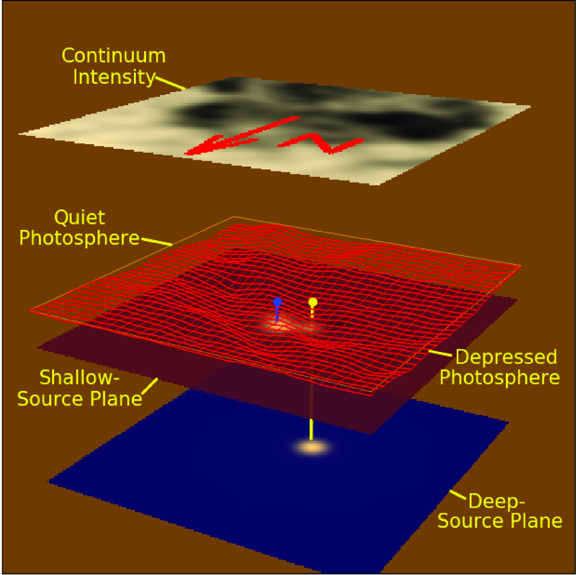
13.4 Case Studies
The first significant sunquake events observed with the HMI instrument were produced on 15 February 2011, by the X2.2-class solar flare (Kosovichev, 2011b; Zharkov et al., 2011, 2013b). The initial flare impacts were observed in the form of compact and rapid variations of the Doppler velocity, line-of-sight magnetic field, and continuum intensity. These variations formed a typical two-ribbon flare structure with two sunquake sources and are believed to be associated with the thermal and hydrodynamic effects of high-energy particles heating the lower atmosphere. The analysis of the SDO/HMI and X-ray data from RHESSI showed that the helioseismic waves might be associated with the photospheric impacts in the early impulsive phase observed before the hard X-ray (50-100 keV) impulse. An acoustic holography analysis applied to the same HMI data deduced that in addition to these (eastern) sunquake sources, there was another weaker (western) source (Zharkov et al., 2011, 2013b). The estimated acoustic energy released was about ergs for the eastern source and ergs for the western source. These estimates are higher than the Lorentz-force energy estimates (Hudson, Fisher, and Welsch, 2008; Alvarado-Gómez et al., 2012b). These observations left open the question of whether the Lorentz force can be a possible mechanism for quake excitation.
The observation of a strong sunquake caused by a compact C7.0 solar flare on 17 February 2013 suggested that the sunquake source might be associated with rapid current dissipation or a localized impulsive Lorentz force in the lower layers of the solar atmosphere because it did not spatially correspond to the strongest hard X-ray emission source (Sharykin, Kosovichev, and Zimovets, 2015). It was the weakest X-ray class flare that produced a significant sunquake. These authors presented another example of a modest X-ray class (M9.3) flare of 30 July 2011, which made a strong photospheric impact and produced a sunquake (Sharykin and Kosovichev, 2015). The absence of CME ruled out magnetic rope eruption as a mechanism of helioseismic waves in this flare. Also, the sunquake impact did not coincide with the strongest HXR source, contradicting the standard beam-driven sunquake generation mechanism. However, the sunquake initiation might be related to the rapid dissipation of electric currents and associated high-speed plasma flows in the lower solar atmosphere during the flare energy release.
Investigations of two homologous X-class flares occurred in the same location with similar morphologies on 6 and 7 September 2011, of which only the first flare produced a sunquake (Zharkov et al., 2013a), suggested that the generation of sunquakes may be explained by a unified model involving simultaneously Lorentz force, hydrodynamic shocks and white light emission, all produced by the magnetic energy released during the flare and its conversion into energetic particles (electrons) with their further effects on a flaring atmosphere and the interior (Xu et al., 2014; Macrae et al., 2018). However, the question of why some flares produce strong photospheric impacts that generate the helioseismic response and others do not is still unresolved.
Fast and complex changes in the magnetic field strength and topology complicate the interpretation of observational data. The reconstruction of magnetic field changes in the solar atmosphere during the M5.7 flare of May 2012 using a non-linear force-free extrapolation and comparison with other flares in the same active region suggested that the sunquake initiation might be associated with the rearrangement of magnetic field lines and strong currents at low altitudes above the polarity boundary line are transformed into the currents along the system of loops oriented at wide angles to the neutral line (Livshits et al., 2016; Grigor’eva and Livshits, 2017). This process may explain the apparent fast supersonic motion of the sunquake sources, originally noticed with the SoHO MDI observations (Kosovichev, 2007) and confirmed by the analysis of sunquakes observed by HMI (Kosovichev, 2011b; Zharkov et al., 2011). The sequential impacts that move along the magnetic arcade can explain the observed anisotropy of the sunquake wavefronts (Kosovichev, 2006a, b).
The X9.3 flare of 6 September 2017, the most powerful flare of Solar Cycle 24, generated strong white-light emission and multiple sunquakes. The photospheric flare impacts started to develop in compact regions near the magnetic polarity inversion line (PIL) in the pre-impulsive phase before detection of the HXR emission. The initial photospheric disturbances were localized in the region of the strong horizontal magnetic field of the PIL and, thus, are likely associated with a compact sheared magnetic structure elongated along the PIL. The acoustic egression power maps revealed two primary sources of sunquake generation, which were associated with places of the strongest photospheric impacts in the pre-impulsive phase and the early impulsive phase (Sharykin and Kosovichev, 2018). Analysis of the high-cadence HMI filtergrams suggests that the flare energy release developed in the form of sequential involvement of compact low-lying magnetic loops that were sheared along the PIL (Livshits et al., 2016). In addition, a second bounce of the generated helioseismic waves detected in this flare was explained by a stronger momentum delivered by the shock generated by a mixed electron-proton beam in the flaring atmosphere and at deeper depths of the interior where this shock was deposited (Zharkova et al., 2020).
The sunquake waves are usually best observed in the frequency range 5-6 mHz as their amplitude rapidly decreases at high frequencies (Zharkov et al., 2013b). Nevertheless, a strong emission at 10 mHz detected in the M9.3 flare of 30 July 2011, (Martínez et al., 2020) was potentially caused by a deep source located about 1 Mm below the solar surface (Lindsey et al., 2020). This result suggested that sunquakes might be caused by perturbations in magnetic subphotospheric layers without producing a compact source signature on the surface (Figure 60). Numerical modeling of deep excitation sources showed the estimated source amplitude is too low to produce the observed wavefront (Stefan and Kosovichev, 2022b).
13.5 Statistical Relationship Among Sunquakes, Magnetic Field Variations, White-Light Emission, and X-ray Emission
Sunquakes represent a critical piece in the broader puzzle of understanding solar flare physics. These helioseismic events provide unique insights into the dynamic processes occurring during some large solar flares, particularly connecting what happens in the low corona and chromosphere with the photosphere and upper sub-photosphere. While sunquakes are invaluable for probing the surface and subsurface seismic impacts of flares, they are only one component of a much broader, complex physical system. A comprehensive understanding of seismically active solar flares requires that sunquakes be studied alongside other key observational phenomena, each offering complementary perspectives on flare dynamics.
Nonthermal hard X-rays, for example, serve as proxies for the dynamics of accelerated electron beams, revealing the distribution and energy of these particles as they precipitate into the lower atmosphere. Magnetic field variations offer another vital piece of the puzzle, providing insights into the magnetic reconnection processes that drive flares and potentially induce Lorentz forces capable of triggering sunquakes. White-light emission, which can account for up to 70% of the total radiated energy during a flare, is thought to be produced through the hydrogen recombination continuum in the upper chromosphere. This emission not only marks intense energy release but also provides clues about the mechanisms behind flare energy dissipation.
Investigating the relationships between sunquakes and other solar flare phenomena can help achieve a more holistic understanding of flare energy transfer processes. When analyzed in conjunction with nonthermal hard X-rays, magnetic field changes, and white-light emission, sunquakes can reveal the intricate interplay between various layers of the solar atmosphere around the photosphere. This multi-observational approach not only deepens our knowledge of sunquakes themselves but also enhances our overall understanding of the physics underlying solar flares.
Before HMI, statistical studies of sunquakes with other flare phenomena were often constrained by small sample sizes, primarily limited to events detected by MDI. The advent of HMI observations has enabled the detection of more sunquakes, and the expanded catalogs allow for more robust statistical studies, providing deeper insights into the complex relationships between sunquakes and other flare-related phenomena. For instance, the relationship between sunquakes, white-light flares, and hard X-ray emissions showed a general correlation between higher electron energy deposition and sunquake occurrence, with seismically active flares often exhibiting harder hard X-ray spectra and more compact source sizes (Pedram and Matthews, 2012). This study found that the link between white-light emission and sunquakes was inconsistent, suggesting that other factors, such as energy distribution and timing, may play crucial roles.
A statistical study of 75 solar flares during Solar Cycle 24, focusing on events with significant hard X-ray (HXR) emissions observed by RHESSI, identified 18 sunquakes, all occurring in flares that exhibited these white-light enhancements. This finding underscores the importance of white-light emission as a marker for sunquake activity and suggests a tight coupling between the energy release processes in the chromosphere and the generation of seismic waves in the photosphere. A later survey of 60 strong flares detected 41 sunquakes, all exhibiting continuum emissions, confirming the association between sunquakes and continuum enhancement (Chen and Zhao, 2021).
A more comprehensive search for sunquakes from 500 M-X class flares during Solar Cycle 24 identified 94 helioseismic events confirmed by at least one detection method (Sharykin and Kosovichev, 2020). This analysis revealed that many moderate-class flares can produce strong sunquakes, while some powerful X-class flares may not be helioseismically active. Notably, the total energy of sunquakes exhibits a stronger correlation with the maximum value of the soft X-ray time derivative than with the X-ray class, indicating that sunquake generation is closely related to the impulsiveness of the energy release. Figure 61 shows the distributions of the seismic and nonseismic flares, between which more evident differences appear in terms of the maximum values of the flare-energy release rate (panel b) than in the GOES class (panel a).
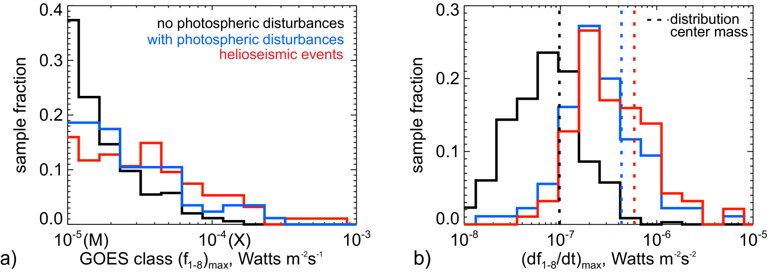
While sunquakes are consistently associated with Doppler transient impacts (sudden perturbations sometimes reaching extreme values in the HMI observables), not all flares with Doppler transients lead to sunquakes (Buitrago-Casas et al., 2015). This suggests that Doppler transients are necessary but not sufficient on their own as a proxy to detect sunquakes, reinforcing the need for a multi-parameter analysis when studying these events (Sharykin and Kosovichev, 2020; Chen and Zhao, 2021). The bottom panels of Figure 56 show examples of Doppler transients at two sunquake source locations, occurring simultaneously with continuum and magnetic field enhancements.
13.6 Imaging Spectro-Polarimetry of Sunquake Sources
The two cameras of the HMI instrument record filtergrams in the linear and circular polarizations in six positions across the spectral line Fe I 6173.34 Å. The filtergrams are used to generate maps of the line width, line depth, Doppler shift, and line-of-sight magnetic field with a 45-sec cadence. In addition, the full Stokes line profiles are calculated with a 90-sec cadence, using the filtergrams from both HMI cameras.
A study of a flare event (SOL-2010-06-12T00:57) found significant blueshifts at both footpoints, while the line remained in absorption (Martínez Oliveros et al., 2011). The blueshifts can be explained by the motion of the photospheric medium toward the observer, which may be caused by various physical phenomena, such as backwarming in the photosphere. The quantitative interpretation of the transient perturbations quantitatively is complicated by the irregular Fe I line shape during flares and requires a detailed radiative transfer modeling taking into account the HMI instrumental characteristics (Sadykov et al., 2020).
A spectro-polarimetric analysis of the first significant sunquake of Solar Cycle 25, observed during the X1.5 flare of 10 May 2022, revealed a transient emission in the line core in three of the four sunquake sources, indicating intense, impulsive heating in the lower chromosphere and photosphere. In addition, the observed variations of the Stokes profiles reflected transient and permanent changes in the magnetic field strength and geometry in the sunquake sources (Figure 57; Kosovichev, Sadykov, and Stefan, 2023). A recent analysis of the HMI spectro-polarimetric observations for the X9.3 flare of 6 September 2017, reveals one or more locations within the sunspot umbra of the associated active region where the Fe I 6173 Å line goes into full emission, indicating significant heating of the photosphere and lower chromosphere. Modeling the HMI observables for ad-hoc heating of the initial empirical umbra model indicated that the line emission in the white-light flare kernels, which coincided with sunquake sources, could be explained by the strong heating of initially cool photospheric regions (Granovsky et al., 2024). However, the current flare models do not explain such strong heating.
13.7 Starquakes
Stellar flares are powerful bursts of energy emitted from the surfaces of stars, possibly caused by the sudden release of magnetic energy in the star’s outer atmosphere. These flares are analogous to solar flares on the Sun but can be far more energetic, especially on stars with more intense magnetic fields, such as red dwarfs, where flares can be particularly powerful and frequent. The sunquakes we observe with HMI do not have sufficient energy to elicit a significant manifestation in individual p-modes (Rabello Soares, Baudin, and Teixeira, 2021). Stellar flares, due to the enormous energy they emit, could be different. The question arises whether the energy they release is sufficient to make the star rings. However, a comparison of the solar-type p-mode spectra of eight stars for periods before and after large flares did not find conclusive evidence that the flares induced global acoustic oscillations (starquakes; Balona et al., 2015).
13.8 Key Questions for Future Studies
Despite the significant progress made in understanding sunquakes and their relationship with various solar flare phenomena, a comprehensive statistical study specifically focusing on the interplay between sunquakes and solar flare magnetic field dynamics is still lacking. Only a handful of studies have examined this relationship in the context of individual flare events, providing valuable but limited insights into the broader picture. These studies, while informative, are not sufficient to establish a robust statistical framework. Moving forward, it is crucial to conduct a systematic statistical study that rigorously investigates the relationship between sunquakes and the magnetic field dynamics of solar flares. Such a study would significantly enhance our understanding of the conditions under which sunquakes are generated and how magnetic field variations influence these seismic events.
The possibility that the sources of flare acoustic transients are submerged opens new mechanisms of acoustic emission, transients that, while triggered by disturbances that originate above the photosphere, are possibly driven by magnetic energy that, like the source, is submerged. If the magnetic energy that is eventually released into the corona causes the flares we see above the photosphere, is it possible for some of this energy to be released into the acoustic field while it has yet to break the surface? This would represent a noteworthy connection with the advent of HMI of two areas of research, flare physics and the solar interior, that, in some ways, have formerly been hermetically separate.
A realistic understanding of the physics of seismic wave generation would in principle teach us a great deal about how flares work, in a context that now extends their mechanics significantly into the solar interior.
14 Solar Irradiance
When the magnetic field generated in the solar interior emerges at the surface of the Sun in a concentrated form, it modifies the radiative properties of the corresponding regions such that some areas on the Sun appear darker (sunspots or pores) or brighter (faculae or network) than the surroundings. This modulates the total solar brightness or irradiance. Thus, analysis and understanding of the variations of solar irradiance provide information on the processes under the solar surface and can, in some ways, be considered complementary to helioseismology.
Solar irradiance is the Sun’s radiative energy flux, measured at the top of Earth’s atmosphere and normalized to the mean Sun-Earth distance. The spectrally-resolved and wavelength-integrated solar irradiance are termed spectral and total solar irradiance (SSI and TSI), respectively.
Due to wavelength- and time-dependent atmospheric absorption and dispersion on the way to the Earth’s surface, measuring irradiance with accuracy sufficient to detect its variability is only possible from space. Direct measurements of TSI and SSI variability exist since 1978 (Fröhlich, 2012) (top panel of Figure 62) and 1967 (though at the beginning over a very limited spectral range only; Ermolli et al., 2013), respectively. They revealed that solar irradiance varies on all observable timescales with a typical amplitude in TSI of about 0.1% over the solar activity cycle and solar rotation timescales (e.g. Kopp, 2016). In the UV, the variations are significantly stronger, reaching several percent in the near- and mid-UV, several tens of percent in the far-UV, and up to about 100% around Ly- (Rottman, 1988; Floyd et al., 2003).
Determining the source of solar irradiance changes and pinpointing its variation in the past (amplitude and timescales of variation) is particularly important for evaluating the solar influence on Earth’s climate. Solar energy is produced in the core of the Sun through nuclear reactions. The chemical evolution of the Sun’s core is important for brightness variations on timescales greater than years. However, on shorter timescales, the energy production in the Sun’s core is considered to be rather stable. Thus, the variations in solar irradiance we observe arise due to changes in how the energy produced in the core reaches the surface of the Sun and how it is radiated from there. The most viable explanation for irradiance variations on timescales from days to millennia lies with changes in the solar surface magnetic field (Shapiro et al., 2017; Yeo et al., 2017). These changes are primarily modulated by the passage of dark sunspots and bright facular and network regions across the solar disk. On shorter timescales, p-mode oscillations peaking at around 5 minutes and granulation are the main drivers of the irradiance fluctuations.
The effect of solar surface magnetic field on irradiance variations has been hypothesized since the very early measurements of irradiance (e.g. Oster, Schatten, and Sofia, 1982; Sofia, Oster, and Schatten, 1982). Sunspots block energy, which is redistributed in the solar convection zone. This stored heat is then re-emitted over the Kelvin-Helmholtz timescale of the convection zone (Spruit, 1982; Domingo et al., 2009; Solanki, Krivova, and Haigh, 2013). This can lead to small variations in the solar radius, which has been suggested to be connected to irradiance variations (Sofia et al., 1979; Sofia, 1998; Pap et al., 2001). A surface radius change of about 0.06 arcseconds (about 45 km) is considered sufficient to account for the 0.1% variation in TSI values over the solar cycle. However, more recent estimates based on SoHO/MDI and SDO/HMI data found significantly smaller changes (Emilio et al., 2000; Kuhn et al., 2004; Jain, Tripathy, and Hill, 2018). This suggests that the radius changes, although interesting in themselves, cannot explain all the TSI variations.
14.1 Irradiance Reconstructions with SDO/HMI Magnetograms
To compute changes in the irradiance caused by magnetic features at the solar surface, models require knowledge about the surface distribution of these features at a given time as well as their brightness or contrast with respect to their quiet surroundings, i.e., regions free of measurable magnetic field. Obviously, the most direct information on the surface distribution of the magnetic field can be retrieved from solar full-disc magnetograms. This information is used by the Spectral and Total Solar irradiance Reconstruction (SATIRE-S, “S” for satellite-era; Krivova et al., 2003) model to reconstruct total and spectral solar irradiance, just as its name suggests. SATIRE-S segments the solar surface into four components: faculae, sunspot umbrae, sunspot penumbrae, and quiet Sun. The brightness of each component is considered time-independent and was computed with the radiative transfer code ATLAS9 (Kurucz, 1970) from the appropriate semi-empirical model atmospheres (Unruh, Solanki, and Fligge, 1999; Tagirov et al., 2019). The brightness depends on the position of the features on the visible solar disc (center-to-limb variation) and the wavelength. In principle, this information can also be extracted from observations. For example, SDO/HMI observations have been used to derive the contrasts of faculae and the network with respect to the quiet Sun as a function of the heliocentric angle and the magnetic field strength (Yeo, Solanki, and Krivova, 2013; Yeo and Krivova, 2019). However, such observation-based contrasts are limited to individual wavelengths and are less reliable close to the solar limb. The latter can be improved by combining observations from different vantage points (Albert et al., 2023) by complementing SDO/HMI observations with data gathered by the Polarimetric and Helioseismic Imager (PHI) (Solanki et al., 2020) onboard Solar Orbiter (SoLo) (Müller et al., 2020). Such information can be used to better constrain the semi-empirical model atmospheres.
The first version of SATIRE-S (Fligge, Solanki, and Unruh, 2000; Krivova et al., 2003) used SoHO/MDI magnetograms and co-temporal continuum images to derive the distribution of the various features on the surface and their evolution with time. Later it was updated to incorporate ground-based magnetograms from the Kitt Peak National Observatory (Wenzler et al., 2004; Wenzler, Solanki, and Krivova, 2005; Wenzler et al., 2006; Ball et al., 2012), followed by SDO/HMI magnetograms and continuum images (Yeo et al., 2014), and most recently also Mt Wilson data. To our knowledge, these are the only irradiance reconstructions employing SDO/HMI magnetograms. Figure 62 shows the complete, most recent SATIRE-S TSI reconstruction along with the one using just SDO/HMI magnetograms and compares them to direct measurements of TSI. In particular, it shows the ROB (named after Royal Observatory of Belgium; Dewitte and Nevens, 2016; Montillet et al., 2022), and the Copernicus Climate Change Service (C3S)171717Available at confluence.ecmwf.int/pages/viewpage.action?pageId=304239361 TSI composites as well as the Total Irradiance Monitor (TIM) onboard the Solar Radiation and Climate Experiment (SORCE/TIM; Kopp and Lawrence, 2005, covering 2003 – 2020) and The Total and Spectral Solar Irradiance Sensor TIM (TSIS1/TIM; Pilewskie et al., 2018, covering 2018 – 2024) direct measurements. The high quality of SDO/HMI magnetograms allows recovering the TSI variations very accurately, reaching linear correlation coefficients (RMS differences) of 0.98 and 0.99 (0.09 and 0.09 Wm-2) when comparing the model with SORCE/TIM and TSIS1/TIM direct TSI measurements, as highlighted in Figure 62.
More recently, co-temporal magnetograms from SDO/HMI and SoLo/PHI were used to reconstruct irradiance variations as seen from two different vantage points (Yeo et al., 2023). Thus, SDO/HMI data also helped to check and calibrate the process of reconstructing irradiance with SO/PHI data, which are obtained from different perspectives than the Sun-Earth line and will eventually also reflect the Sun as seen from outside ecliptic plane, from heliolatitudes of up to 33∘.
14.2 Using SDO/HMI Magnetograms to Verify the Magnetic Origin of Irradiance Variations
A limitation of nearly all existing irradiance models is that they have free parameters they need to fix by comparing to irradiance measurements. The first and, until now, the only irradiance model that does not require any tuning to the measured irradiance variations was produced by employing three-dimensional MHD MURaM (Vögler et al., 2005) simulations of the solar atmosphere (Yeo et al., 2017). The model produced bolometric images based on the active region distribution found in SDO/HMI magnetograms and achieved an excellent agreement to measured TSI, reaching linear correlation coefficients (RMS differences) of 0.99 (0.07 and 0.09 Wm-2) compared to SORCE/TIM and TSIS1/TIM direct measurements (Chatzistergos, Krivova, and Yeo, 2023). It demonstrated that solar surface magnetism accounts for almost all irradiance variations on time scales of days to the solar cycle, leaving very little room for other mechanisms (Shapiro et al., 2017).
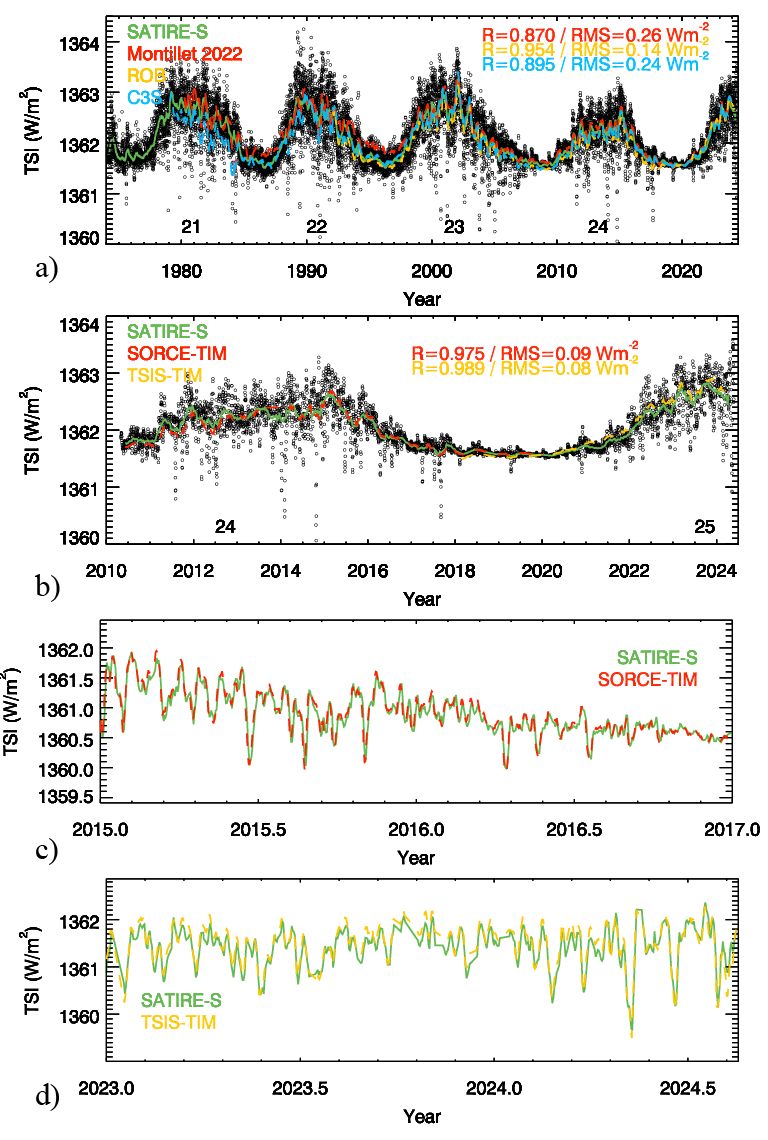
14.3 Irradiance Variations on Longer Timescales
While covering only the last 1.5 solar cycles (Solar Cycle 24 and the first half of Cycle 25), SDO/HMI observations are also useful for constraining, even if indirectly, the longer-term changes in the irradiance, which is one of the key open questions in irradiance reconstructions. Solar full-disc magnetograms have only been available for roughly half a century. Assessment of the Sun’s impact on the Earth’s climate requires significantly longer records. Reconstructions of solar irradiance variations at earlier times are mostly based on sunspot observations or cosmogenic isotope data (Solanki and Fligge, 1999; Krivova, Balmaceda, and Solanki, 2007; Krivova, Vieira, and Solanki, 2010; Vieira et al., 2011; Wu et al., 2018; Chatzistergos, 2024). These data, however, do not provide direct information on the evolution of the faculae and the network, which are thought to be the main drivers of the variability on time scales of the solar cycle and longer. This limitation led to significant uncertainty, by about a factor of 10, in the magnitude of the secular irradiance change (e.g., Solanki, Krivova, and Haigh, 2013; Chatzistergos, Krivova, and Yeo, 2023). This problem can be addressed by using historical archives of full-disc solar photographs in the Ca ii K line. Such observations constitute the second-longest photographic archive of solar observations after white-light observations. Observations in the Ca ii K line started in 1892 and continue to this day at various sites around the world (Chatzistergos et al., 2020; Chatzistergos, Krivova, and Ermolli, 2022). It has been shown that solar brightness in the Ca ii K line is an excellent tracer of the Sun’s magnetic activity (e.g. Schrijver et al., 1989; Loukitcheva, Solanki, and White, 2009; Kahil, Riethmüller, and Solanki, 2017).
The relationship between the solar surface magnetic field strength and the brightness in the Ca ii K line core derived from near-co-temporal Rome Ca ii K observations (Ermolli, Giorgi, and Chatzistergos, 2022) and SDO/HMI magnetograms was then used to recover unsigned magnetograms (Chatzistergos et al., 2019) from which solar irradiance was reconstructed (Chatzistergos et al., 2021; Chatzistergos, Krivova, and Ermolli, 2024). For example, three Ca ii K archives (Meudon, Rome, and San Fernando) were used in the SATIRE-S composite series shown in the top panel of Figure 62 to fill gaps in the reconstruction left by the direct magnetogram sources. This paved the way to reconstruct unsigned magnetograms from historical Ca ii K observations back to the late 19th century. Solar irradiance can sometimes be reconstructed before directly measured magnetograms become available. Since TSI reconstructions from the combination of sunspots and such reconstructed magnetograms have been far more reliable than reconstructions based on sunspots alone, we expect that this work will help settle the issue of the increase in TSI since the Maunder minimum.
Conclusions, Challenges, and Unresolved Problems
The high-resolution uninterrupted data from the Helioseismic and Magnetic Imager substantially advanced our knowledge of the solar structure and activity. They have stimulated the development of new helioseismic techniques, such as high-resolution mapping of subsurface flows by local helioseismology, accurate detection of active regions in the solar interior and far side of the Sun, imaging of the zonal and meridional flows in the whole convection zone, high-precision measurements of the solar tachocline and the near-surface shear layer, and analysis of large-scale complex flows using the novel mode coupling technique, which led to discovery of global Rossby waves.
As a result of these investigations, a new, highly dynamic picture of the Sun is emerging. It is characterized by strong multi-scale interaction of convective flows, differential rotation, global circulation, and magnetic fields. Although the first attempts to measure subsurface magnetic fields have been made, most of our knowledge about the physical processes inside the Sun comes from the flow measurements. In particular, the measurements of the migrating zonal and meridional flows provided evidence for dynamo waves and showed the Near-Surface Shear Layer (NSSL) plays an important role in the solar dynamo and activity cycles. The local helioseismology analysis of subsurface convection revealed the co-existence of multi-scale flows, from supergranulation to giant cells, challenging the classical mixing-length theory of stellar convection. It appears that large-scale convection is linked to Rossby-type waves, creating complicated global flow patterns in the equatorial and polar regions.
The data analysis and supporting numerical simulation revealed the ‘leptocline’, a highly dynamical shallow substructure of the NSSL in the top 5-10 Mm of the convection zone. It is found that both the zonal and meridional flows vary with the ‘extended’ 22-year solar cycle, and the branches of these flows continue to migrate towards the equator even during the deep minimum of solar activity when no significant magnetic field is observed on the surface, meaning that these variations are driven by subsurface processes, associated with the solar dynamo. During the solar maxima, the zonal and meridional flows interact with converging flows formed around magnetic active regions in the leptocline affecting the meridional flux transport and creating complicated ‘Solar Subsurface Weather’ (SSW) patterns. The data suggest that the subsurface converging and shearing flows in active regions may play a critical role in their flaring and CME activity. Measuring characteristics of these flows (such as divergence and vorticity) and properties of solar oscillations (distribution of the surface power and mode amplitude) may help predict the emergence of sunspot regions and their activity.
The interaction of subsurface flows with magnetic fields is also critical for understanding the energy flow inside the Sun. Current state-of-the-art physics-based irradiance models (e.g., SATIRE-3D; Section 14) can explain the measured solar irradiance variations from the surface magnetograms, leaving no room for any additional contributions. At this stage, however, the influence of subsurface dynamics over timescales significantly longer than those covered by irradiance measurements cannot be ruled out.
In terms of acoustic energy transport, the helioseismology data revealed enhanced power of high-frequency acoustic waves (’acoustic halos’) around sunspot regions. In particular, the HMI observations detected a double-ring structure of the power enhancement, which is explained by wave transformation in high-intensity magnetic fields. The halos can contribute to coronal heating in active regions. It was known that solar acoustic oscillations are excited in intergranular lanes close to the surface, but the HMI observations revealed deep acoustic sources beneath sunspot regions at a depth of about 5 Mm. Numerical simulations showed that these sources may be caused by the interaction of magnetic field bundles.
It is intriguing that the acoustic holography method detected deep (‘submerged’) acoustic sources associated with helioseismic waves excited during solar flares (’sunquakes’). The HMI showed that sunquakes are more frequent than was thought before and can be produced by relatively weak flares (in terms of the X-ray flux). It was found that the sunquakes are produced by compact impulsive flares at the beginning of their impulsive phase and that their sources are associated with continuum (white-light) emission, Doppler velocity transients, and permanent or transient magnetic field variations. Although the physical mechanism of sunquake sources has not been established, recent radiative hydrodynamic and acoustic models indicate that sunquakes may be caused by deeply penetrating proton beams. Thus, the origin of sunquakes is closely related to the fundamental problem of the flare energy release and transport.
The HMI advances raised new challenges, and many problems remain unsolved. In particular, it is important to implement high-degree helioseismology data analysis and inversion procedures, which will substantially improve the spatial resolution of the solar structure and rotation in the near-surface shear layer. In addition, it is critical for solar dynamics and dynamo modeling to measure the spectrum of solar convection with higher accuracy to solve ‘the convective conundrum’ problem - a large discrepancy among various local helioseismology measurement techniques and numerical models. The deep structure of the meridional circulation and its variations with the solar cycle (particularly at the base of the solar convection zone and high latitudes), which is still a highly debated problem, is also a critical element of dynamo theories. Its solution depends on improving our understanding of the center-to-limb variations of acoustic travel times. The recently discovered Rossby waves potentially play an important role in the solar structure, dynamics, and magnetic activity. Another unsolved problem that may significantly improve space weather forecasts is the helioseismic diagnostics of emerging and evolving active regions on the front and far sides of the Sun. In addition, the challenges in understanding solar composition, variations in solar irradiance, and sunquake sources are deeply connected to fundamental problems of physics and astrophysics. The future development of this field requires a synergy of new sophisticated data analysis techniques and realistic modeling and simulations.
The HMI instrument continues providing high-quality data that undoubtedly will lead to new discoveries. We also anticipate that new out-of-ecliptic observations of solar polar regions from Solar Orbiter, which is currently in operation, and the planned Solaris mission will complement the HMI observations and allow us to complete the global dynamic picture of the solar interior.
Acknowledgments. This work utilizes data from HMI onboard NASA’s SDO spacecraft, courtesy of NASA/SDO and the HMI Science Teams. It also utilizes data from the MDI onboard SoHO. SoHO is a mission of international cooperation between ESA and NASA. This work also utilizes GONG data obtained by the NSO Integrated Synoptic Program, managed by the National Solar Observatory, which is operated by the Association of Universities for Research in Astronomy (AURA), Inc. under a cooperative agreement with the National Science Foundation (NSF) and with contribution from the National Oceanic and Atmospheric Administration (NOAA). The GONG network of instruments is hosted by the Big Bear Solar Observatory, High Altitude Observatory, Learmonth Solar Observatory, Udaipur Solar Observatory, Instituto de Astrofísica de Canarias, and Cerro Tololo Interamerican Observatory. 10.7 cm radio flux data is provided by the National Resources Canada (NRC) Space Weather. Resources supporting this work were provided by the NASA High-End Computing (HEC) Program through the NASA Advanced Supercomputing (NAS) Division at Ames Research Center. This research has used NASA’s Astrophysics Data System (ADS: ui.adsabs.harvard.edu/) Bibliographic Services.
This work is partially supported by the NASA Contract NAS5-02139, NASA grants 80NSSC20K0602, 80NSSC22M0162, 80NSSC20K0194, 80NSSC21K0735, 80NSSC23K0563, 80NSSC23K0404, 80NSSC22K0516, 80NSSC19K0268, 80NSSC20K1320, 80NSSC19K1436, 80NSSC23K0097, and NSF grant 1916509. This project has received funding from the European Research Council (ERC) under the European Union’s Horizon 2020 research and innovation program (grant agreement No. 101097844 — project WINSUN), the UK Science and Technology Facilities Council (STFC) through grant ST/V000500/1, and the GOLF and PLATO Centre National D’Études Spatiales grants.
References
- Albert et al. (2023) Albert, K., Krivova, N.A., Hirzberger, J., Solanki, S.K., et al.: 2023, Intensity contrast of solar network and faculae close to the solar limb, observed from two vantage points. Astron. Astrophys. 678, A163. DOI.
- Allred et al. (2005) Allred, J.C., Hawley, S.L., Abbett, W.P., Carlsson, M.: 2005, Radiative Hydrodynamic Models of the Optical and Ultraviolet Emission from Solar Flares. ApJ 630, 573. DOI. ADS.
- Alvarado-Gómez et al. (2012a) Alvarado-Gómez, J.D., Buitrago-Casas, J.C., Martínez-Oliveros, J.C., Lindsey, C., Hudson, H., Calvo-Mozo, B.: 2012a, Magneto-Acoustic Energetics Study of the Seismically Active Flare of 15 February 2011. Sol. Phys. 280, 335. DOI. ADS.
- Alvarado-Gómez et al. (2012b) Alvarado-Gómez, J.D., Buitrago-Casas, J.C., Martínez-Oliveros, J.C., Lindsey, C., Hudson, H., Calvo-Mozo, B.: 2012b, Magneto-Acoustic Energetics Study of the Seismically Active Flare of 15 February 2011. Sol. Phys. 280, 335. DOI. ADS.
- Angus et al. (2015) Angus, R., Aigrain, S., Foreman-Mackey, D., McQuillan, A.: 2015, Calibrating gyrochronology using Kepler asteroseismic targets. MNRAS 450, 1787. DOI. ADS.
- Antia (1998) Antia, H.M.: 1998, Estimate of solar radius from f-mode frequencies. A&A 330, 336. DOI. ADS.
- Antia and Basu (2022) Antia, H.M., Basu, S.: 2022, Changes in the Near-surface Shear Layer of the Sun. ApJ 924, 19. DOI. ADS.
- Antia, Basu, and Chitre (1998) Antia, H.M., Basu, S., Chitre, S.M.: 1998, Solar internal rotation rate and the latitudinal variation of the tachocline. MNRAS 298, 543. DOI. ADS.
- Antia, Chitre, and Thompson (2003) Antia, H.M., Chitre, S.M., Thompson, M.J.: 2003, On variation of the latitudinal structure of the solar convection zone. A&A 399, 329. DOI. ADS.
- Antia et al. (2000) Antia, H.M., Basu, S., Pintar, J., Pohl, B.: 2000, Solar Cycle Variation in Solar f-Mode Frequencies and Radius. Sol. Phys. 192, 459. DOI. ADS.
- Antia et al. (2001) Antia, H.M., Basu, S., Hill, F., Howe, R., Komm, R.W., Schou, J.: 2001, Solar-cycle variation of the sound-speed asphericity from GONG and MDI data 1995-2000. MNRAS 327, 1029. DOI. ADS.
- Anwar et al. (1993) Anwar, B., Acton, L.W., Hudson, H.S., Makita, M., McClymont, A.N., Tsuneta, S.: 1993, Rapid Sunspot Motion during a Major Solar Flare. Sol. Phys. 147, 287.
- Appourchaux et al. (2008) Appourchaux, T., Michel, E., Auvergne, M., Baglin, A., Toutain, T., Baudin, F., Benomar, O., Chaplin, W.J., Deheuvels, S., Samadi, R., Verner, G.A., Boumier, P., García, R.A., Mosser, B., Hulot, J.-C., Ballot, J., Barban, C., Elsworth, Y., Jiménez-Reyes, S.J., Kjeldsen, H., Régulo, C., Roxburgh, I.W.: 2008, CoRoT sounds the stars: p-mode parameters of Sun-like oscillations on HD 49933. A&A 488, 705. DOI. ADS.
- Arge et al. (2013) Arge, C.N., Henney, C.J., Hernandez, I.G., Toussaint, W.A., Koller, J., Godinez, H.C.: 2013, Modeling the corona and solar wind using ADAPT maps that include far-side observations. In: Zank, G.P., Borovsky, J., Bruno, R., Cirtain, J., Cranmer, S., Elliott, H., Giacalone, J., Gonzalez, W., Li, G., Marsch, E., Moebius, E., Pogorelov, N., Spann, J., Verkhoglyadova, O. (eds.) Solar Wind 13, American Institute of Physics Conference Series 1539, AIP, 11. DOI. ADS.
- Asplund, Amarsi, and Grevesse (2021) Asplund, M., Amarsi, A.M., Grevesse, N.: 2021, The chemical make-up of the Sun: A 2020 vision. A&A 653, A141. DOI. ADS.
- Asplund, Grevesse, and Sauval (2005) Asplund, M., Grevesse, N., Sauval, A.J.: 2005, The Solar Chemical Composition. In: Barnes, I. Thomas G., Bash, F.N. (eds.) Cosmic Abundances as Records of Stellar Evolution and Nucleosynthesis, Astronomical Society of the Pacific Conference Series 336, 25. ADS.
- Attie and Innes (2015) Attie, R., Innes, D.E.: 2015, Magnetic balltracking: Tracking the photospheric magnetic flux. A&A 574, A106. DOI. ADS.
- Attie et al. (2018) Attie, R., Kirk, M.S., Thompson, B.J., Muglach, K., Norton, A.A.: 2018, Precursors of Magnetic Flux Emergence in the Moat Flows of Active Region AR12673. Space Weather 16, 1143. DOI. ADS.
- Backus and Gilbert (1968) Backus, G., Gilbert, F.: 1968, The Resolving Power of Gross Earth Data. Geophys. J. 16, 169. DOI. ADS.
- Baglin et al. (2006) Baglin, A., Auvergne, M., Boisnard, L., Lam-Trong, T., Barge, P., Catala, C., Deleuil, M., Michel, E., Weiss, W.: 2006, CoRoT: a high precision photometer for stellar ecolution and exoplanet finding. In: 36th COSPAR Scientific Assembly, COSPAR, Plenary Meeting 36, 3749. ADS.
- Bailey et al. (2015) Bailey, J.E., Nagayama, T., Loisel, G.P., Rochau, G.A., Blancard, C., Colgan, J., Cosse, P., Faussurier, G., Fontes, C.J., Gilleron, F., Golovkin, I., Hansen, S.B., Iglesias, C.A., Kilcrease, D.P., Macfarlane, J.J., Mancini, R.C., Nahar, S.N., Orban, C., Pain, J.-C., Pradhan, A.K., Sherrill, M., Wilson, B.G.: 2015, A higher-than-predicted measurement of iron opacity at solar interior temperatures. Nature 517, 56. DOI. ADS.
- Baird, Tripathy, and Jain (2024) Baird, M.A., Tripathy, S.C., Jain, K.: 2024, Connection between Subsurface Layers and Surface Magnetic Activity over Multiple Solar Cycles Using GONG Observations. ApJ 962, 194. DOI. ADS.
- Baldner and Basu (2008) Baldner, C.S., Basu, S.: 2008, Solar Cycle Related Changes at the Base of the Convection Zone. ApJ 686, 1349. DOI. ADS.
- Baldner and Schou (2012) Baldner, C.S., Schou, J.: 2012, Effects of Asymmetric Flows in Solar Convection on Oscillation Modes. ApJ 760, L1. DOI. ADS.
- Ball and Gizon (2014) Ball, W.H., Gizon, L.: 2014, A new correction of stellar oscillation frequencies for near-surface effects. A&A 568, A123. DOI. ADS.
- Ball et al. (2012) Ball, W.T., Unruh, Y.C., Krivova, N.A., Solanki, S., Wenzler, T., Mortlock, D.J., Jaffe, A.H.: 2012, Reconstruction of total solar irradiance 1974-2009. Astron. Astrophys. 541, A27. DOI.
- Ballot, García, and Lambert (2006) Ballot, J., García, R.A., Lambert, P.: 2006, Rotation speed and stellar axis inclination from p modes: how CoRoT would see other suns. MNRAS 369, 1281. DOI. ADS.
- Ballot et al. (2011) Ballot, J., Gizon, L., Samadi, R., Vauclair, G., Benomar, O., Bruntt, H., Mosser, B., Stahn, T., Verner, G.A., Campante, T.L., García, R.A., Mathur, S., Salabert, D., Gaulme, P., Régulo, C., Roxburgh, I.W., Appourchaux, T., Baudin, F., Catala, C., Chaplin, W.J., Deheuvels, S., Michel, E., Bazot, M., Creevey, O., Dolez, N., Elsworth, Y., Sato, K.H., Vauclair, S., Auvergne, M., Baglin, A.: 2011, Accurate p-mode measurements of the G0V metal-rich CoRoT target HD 52265. A&A 530, A97. DOI. ADS.
- Balona et al. (2015) Balona, L.A., Broomhall, A.-M., Kosovichev, A., Nakariakov, V.M., Pugh, C.E., Van Doorsselaere, T.: 2015, Oscillations in stellar superflares. MNRAS 450, 956. DOI. ADS.
- Barekat, Schou, and Gizon (2014) Barekat, A., Schou, J., Gizon, L.: 2014, The radial gradient of the near-surface shear layer of the Sun. A&A 570, L12. DOI. ADS.
- Barekat, Schou, and Gizon (2016) Barekat, A., Schou, J., Gizon, L.: 2016, Solar-cycle variation of the rotational shear near the solar surface. A&A 595, A8. DOI. ADS.
- Barnes (2007) Barnes, S.A.: 2007, Ages for Illustrative Field Stars Using Gyrochronology: Viability, Limitations, and Errors. ApJ 669, 1167. DOI. ADS.
- Barnes et al. (2016) Barnes, S.A., Weingrill, J., Fritzewski, D., Strassmeier, K.G., Platais, I.: 2016, Rotation Periods for Cool Stars in the 4 Gyr old Open Cluster M67, The Solar Stellar Connection, and the Applicability of Gyrochronology to at least Solar Age. ApJ 823, 16. DOI. ADS.
- Basu (1997) Basu, S.: 1997, Seismology of the base of the solar convection zone. MNRAS 288, 572. DOI. ADS.
- Basu (2016) Basu, S.: 2016, Global seismology of the Sun. Living Rev. Solar Phys. 13, 2. DOI. ADS.
- Basu (2021) Basu, S.: 2021, Evidence of Solar-cycle-related Structural Changes in the Solar Convection Zone. ApJ 917, 45. DOI. ADS.
- Basu and Antia (1995) Basu, S., Antia, H.M.: 1995, Helium abundance in the solar envelope. MNRAS 276, 1402. DOI. ADS.
- Basu and Antia (1999) Basu, S., Antia, H.M.: 1999, Large-Scale Flows in the Solar Interior: Effect of Asymmetry in Peak Profiles. ApJ 525, 517. DOI. ADS.
- Basu and Antia (2001) Basu, S., Antia, H.M.: 2001, A study of possible temporal and latitudinal variations in the properties of the solar tachocline. MNRAS 324, 498. DOI. ADS.
- Basu and Antia (2008) Basu, S., Antia, H.M.: 2008, Helioseismology and solar abundances. Phys. Rep. 457, 217. DOI. ADS.
- Basu and Antia (2019) Basu, S., Antia, H.M.: 2019, Changes in Solar Rotation over Two Solar Cycles. ApJ 883, 93. DOI. ADS.
- Basu and Korzennik (2024) Basu, S., Korzennik, S.G.: 2024, Asphericity of the Base of the Solar Convection Zone. ApJ 964, 8. DOI. ADS.
- Basu and Mandel (2004) Basu, S., Mandel, A.: 2004, Does Solar Structure Vary with Solar Magnetic Activity? ApJ 617, L155. DOI. ADS.
- Basu, Däppen, and Nayfonov (1999) Basu, S., Däppen, W., Nayfonov, A.: 1999, Helioseismic Analysis of the Hydrogen Partition Function in the Solar Interior. ApJ 518, 985. DOI. ADS.
- Bazot et al. (2018) Bazot, M., Nielsen, M.B., Mary, D., Christensen-Dalsgaard, J., Benomar, O., Petit, P., Gizon, L., Sreenivasan, K.R., White, T.R.: 2018, Butterfly diagram of a Sun-like star observed using asteroseismology. A&A 619, L9. DOI. ADS.
- Bazot et al. (2019) Bazot, M., Benomar, O., Christensen-Dalsgaard, J., Gizon, L., Hanasoge, S., Nielsen, M., Petit, P., Sreenivasan, K.R.: 2019, Latitudinal differential rotation in the solar analogues 16 Cygni A and B. A&A 623, A125. DOI. ADS.
- Beaudoin et al. (2013) Beaudoin, P., Charbonneau, P., Racine, E., Smolarkiewicz, P.K.: 2013, Torsional Oscillations in a Global Solar Dynamo. Sol. Phys. 282, 335. DOI. ADS.
- Beck, Duvall, and Scherrer (1998) Beck, J.G., Duvall, T.L., Scherrer, P.H.: 1998, Long-lived giant cells detected at the surface of the Sun. Nature 394, 653. DOI. ADS.
- Bekki (2024) Bekki, Y.: 2024, Numerical study of non-toroidal inertial modes with l = m + 1 radial vorticity in the Sun’s convection zone. A&A 682, A39. DOI. ADS.
- Bekki, Cameron, and Gizon (2022a) Bekki, Y., Cameron, R.H., Gizon, L.: 2022a, Theory of solar oscillations in the inertial frequency range: Amplitudes of equatorial modes from a nonlinear rotating convection simulation. A&A 666, A135. DOI. ADS.
- Bekki, Cameron, and Gizon (2022b) Bekki, Y., Cameron, R.H., Gizon, L.: 2022b, Theory of solar oscillations in the inertial frequency range: Linear modes of the convection zone. A&A 662, A16. DOI. ADS.
- Bekki, Cameron, and Gizon (2024) Bekki, Y., Cameron, R.H., Gizon, L.: 2024, The Sun’s differential rotation is controlled by high-latitude baroclinically unstable inertial modes. Science Adv. 10, eadk5643. DOI. ADS.
- Bellinger and Christensen-Dalsgaard (2022) Bellinger, E.P., Christensen-Dalsgaard, J.: 2022, Towards solar measurements of nuclear reaction rates. MNRAS 517, 5281. DOI. ADS.
- Bellinger et al. (2023) Bellinger, E.P., Caplan, M.E., Ryu, T., Bollimpalli, D., Ball, W.H., Kühnel, F., Farmer, R., de Mink, S.E., Christensen-Dalsgaard, J.: 2023, Solar Evolution Models with a Central Black Hole. ApJ 959, 113. DOI. ADS.
- Benevolenskaya (1998) Benevolenskaya, E.E.: 1998, A Model of the Double Magnetic Cycle of the Sun. ApJ 509, L49. DOI. ADS.
- Benomar et al. (2009) Benomar, O., Baudin, F., Campante, T.L., Chaplin, W.J., García, R.A., Gaulme, P., Toutain, T., Verner, G.A., Appourchaux, T., Ballot, J., Barban, C., Elsworth, Y., Mathur, S., Mosser, B., Régulo, C., Roxburgh, I.W., Auvergne, M., Baglin, A., Catala, C., Michel, E., Samadi, R.: 2009, A fresh look at the seismic spectrum of HD49933: analysis of 180 days of CoRoT photometry. A&A 507, L13. DOI. ADS.
- Benomar et al. (2018) Benomar, O., Bazot, M., Nielsen, M.B., Gizon, L., Sekii, T., Takata, M., Hotta, H., Hanasoge, S., Sreenivasan, K.R., Christensen-Dalsgaard, J.: 2018, Asteroseismic detection of latitudinal differential rotation in 13 Sun-like stars. Science 361, 1231. DOI. ADS.
- Benomar et al. (2023) Benomar, O., Takata, M., Bazot, M., Sekii, T., Gizon, L., Lu, Y.: 2023, Detecting active latitudes of Sun-like stars using asteroseismic a-coefficients. A&A 680, A27. DOI. ADS.
- Bétrisey et al. (2024) Bétrisey, J., Farnir, M., Breton, S.N., García, R.A., Broomhall, A.-M., Amarsi, A.M., Kochukhov, O.: 2024, Imprint of the magnetic activity cycle on solar asteroseismic characterisation based on 26 years of GOLF and BiSON data. A&A 688, L17. DOI. ADS.
- Bhattacharya and Hanasoge (2023) Bhattacharya, J., Hanasoge, S.M.: 2023, A Spectral Solver for Solar Inertial Waves. ApJS 264, 21. DOI. ADS.
- Bhattacharya et al. (2024) Bhattacharya, J., Hanson, C.S., Hanasoge, S.M., Sreenivasan, K.R.: 2024, A Linear Model for Inertial Modes in a Differentially Rotating Sun. ApJ 965, 55. DOI. ADS.
- Birch and Gizon (2007) Birch, A.C., Gizon, L.: 2007, Linear sensitivity of helioseismic travel times to local flows. Astron. Nachr. 328, 228. DOI. ADS.
- Birch and Kosovichev (2000) Birch, A.C., Kosovichev, A.G.: 2000, Travel Time Sensitivity Kernels. Sol. Phys. 192, 193. DOI. ADS.
- Birch, Braun, and Fan (2010) Birch, A.C., Braun, D.C., Fan, Y.: 2010, An Estimate of the Detectability of Rising Flux Tubes. ApJ 723, L190. DOI. ADS.
- Birch, Kosovichev, and Duvall (2004) Birch, A.C., Kosovichev, A.G., Duvall, J. T. L.: 2004, Sensitivity of Acoustic Wave Travel Times to Sound-Speed Perturbations in the Solar Interior. ApJ 608, 580. DOI. ADS.
- Birch et al. (2011) Birch, A.C., Parchevsky, K.V., Braun, D.C., Kosovichev, A.G.: 2011, “Hare and Hounds” Tests of Helioseismic Holography. Sol. Phys. 272, 11. DOI. ADS.
- Birch et al. (2013) Birch, A.C., Braun, D.C., Leka, K.D., Barnes, G., Javornik, B.: 2013, Helioseismology of Pre-emerging Active Regions. II. Average Emergence Properties. ApJ 762, 131. DOI. ADS.
- Birch et al. (2016) Birch, A.C., Schunker, H., Braun, D.C., Cameron, R., Gizon, L., Loptien, B., Rempel, M.: 2016, A low upper limit on the subsurface rise speed of solar active regions. Sci. Adv. 2, e1600557. DOI. ADS.
- Blume, Hindman, and Matilsky (2024) Blume, C.C., Hindman, B.W., Matilsky, L.I.: 2024, Inertial Waves in a Nonlinear Simulation of the Sun’s Convection Zone and Radiative Interior. ApJ 966, 29. DOI. ADS.
- Bogart, Baldner, and Basu (2015) Bogart, R.S., Baldner, C.S., Basu, S.: 2015, Evolution of Near-surface Flows Inferred from High-resolution Ring-diagram Analysis. ApJ 807, 125. DOI. ADS.
- Bogart et al. (2011a) Bogart, R.S., Baldner, C., Basu, S., Haber, D.A., Rabello-Soares, M.C.: 2011a, HMI ring diagram analysis I. The processing pipeline. In: GONG-SoHO 24: A New Era of Seismology of the Sun and Solar-Like Stars, 271, IOP, 012008. DOI. ADS.
- Bogart et al. (2011b) Bogart, R.S., Baldner, C., Basu, S., Haber, D.A., Rabello-Soares, M.C.: 2011b, HMI ring diagram analysis II. Data products. In: GONG-SoHO 24: A New Era of Seismology of the Sun and Solar-Like Stars, 271, IOP, 012009. DOI. ADS.
- Bogart et al. (2023) Bogart, R.S., Baldner, C.S., Basu, S., Howe, R., Rabello Soares, M.C.: 2023, Evidence of a Quasiperiodic Global-scale Oscillation in the Near-surface Shear Layer of the Sun. ApJ 950, L21. DOI. ADS.
- Böning et al. (2016) Böning, V.G.A., Roth, M., Zima, W., Birch, A.C., Gizon, L.: 2016, Sensitivity Kernels for Flows in Time-Distance Helioseismology: Extension to Spherical Geometry. ApJ 824, 49. DOI. ADS.
- Böning et al. (2017) Böning, V.G.A., Roth, M., Jackiewicz, J., Kholikov, S.: 2017, Inversions for Deep Solar Meridional Flow Using Spherical Born Kernels. ApJ 845, 2. DOI. ADS.
- Borexino Collaboration et al. (2020) Borexino Collaboration, M. Agostini, Altenmüller, K., Appel, S., Atroshchenko, V., Bagdasarian, Z., Basilico, D., Bellini, G., Benziger, J., Biondi, R., Bravo, D., Caccianiga, B., Calaprice, F., Caminata, A., Cavalcante, P., Chepurnov, A., D’Angelo, D., Davini, S., Derbin, A., Di Giacinto, A., Di Marcello, V., Ding, X.F., Di Ludovico, A., Di Noto, L., Drachnev, I., Formozov, A., Franco, D., Galbiati, C., Ghiano, C., Giammarchi, M., Goretti, A., Göttel, A.S., Gromov, M., Guffanti, D., Ianni, A., Ianni, A., Jany, A., Jeschke, D., Kobychev, V., Korga, G., Kumaran, S., Laubenstein, M., Litvinovich, E., Lombardi, P., Lomskaya, I., Ludhova, L., Lukyanchenko, G., Lukyanchenko, L., Machulin, I., Martyn, J., Meroni, E., Meyer, M., Miramonti, L., Misiaszek, M., Muratova, V., Neumair, B., Nieslony, M., Nugmanov, R., Oberauer, L., Orekhov, V., Ortica, F., Pallavicini, M., Papp, L., Pelicci, L., Penek, Ö., Pietrofaccia, L., Pilipenko, N., Pocar, A., Raikov, G., Ranalli, M.T., Ranucci, G., Razeto, A., Re, A., Redchuk, M., Romani, A., Rossi, N., Schönert, S., Semenov, D., Settanta, G., Skorokhvatov, M., Singhal, A., Smirnov, O., Sotnikov, A., Suvorov, Y., Tartaglia, R., Testera, G., Thurn, J., Unzhakov, E., Villante, F.L., Vishneva, A., Vogelaar, R.B., von Feilitzsch, F., Wojcik, M., Wurm, M., Zavatarelli, S., Zuber, K., Zuzel, G.: 2020, Experimental evidence of neutrinos produced in the CNO fusion cycle in the Sun. Nature 587, 577. DOI. ADS.
- Borucki et al. (2010) Borucki, W.J., Koch, D., Basri, G., Batalha, N., Brown, T., Caldwell, D., Caldwell, J., Christensen-Dalsgaard, J., Cochran, W.D., DeVore, E., Dunham, E.W., Dupree, A.K., Gautier, T.N., Geary, J.C., Gilliland, R., Gould, A., Howell, S.B., Jenkins, J.M., Kondo, Y., Latham, D.W., Marcy, G.W., Meibom, S., Kjeldsen, H., Lissauer, J.J., Monet, D.G., Morrison, D., Sasselov, D., Tarter, J., Boss, A., Brownlee, D., Owen, T., Buzasi, D., Charbonneau, D., Doyle, L., Fortney, J., Ford, E.B., Holman, M.J., Seager, S., Steffen, J.H., Welsh, W.F., Rowe, J., Anderson, H., Buchhave, L., Ciardi, D., Walkowicz, L., Sherry, W., Horch, E., Isaacson, H., Everett, M.E., Fischer, D., Torres, G., Johnson, J.A., Endl, M., MacQueen, P., Bryson, S.T., Dotson, J., Haas, M., Kolodziejczak, J., Van Cleve, J., Chandrasekaran, H., Twicken, J.D., Quintana, E.V., Clarke, B.D., Allen, C., Li, J., Wu, H., Tenenbaum, P., Verner, E., Bruhweiler, F., Barnes, J., Prsa, A.: 2010, Kepler Planet-Detection Mission: Introduction and First Results. Science 327. DOI. ADS.
- Braun (1995) Braun, D.C.: 1995, Scattering of p-Modes by Sunspots. I. Observations. ApJ 451, 859. DOI. ADS.
- Braun (2012) Braun, D.C.: 2012, Comment on “Detection of Emerging Sunspot Regions in the Solar Interior”. Science 336, 296. DOI. ADS.
- Braun (2019) Braun, D.C.: 2019, Flows around Averaged Solar Active Regions. ApJ 873, 94. DOI. ADS.
- Braun (2024) Braun, D.C.: 2024, The Contribution of Solar Magnetic Regions to the Residual Meridional and Zonal Flows. ApJ 972, 160. DOI. ADS.
- Braun and Fan (1998) Braun, D.C., Fan, Y.: 1998, Helioseismic Measurements of the Subsurface Meridional Flow. ApJ 508, L105. DOI. ADS.
- Braun and Lindsey (2001) Braun, D.C., Lindsey, C.: 2001, Seismic Imaging of the Far Hemisphere of the Sun. ApJ 560, L189. DOI. ADS.
- Braun, Birch, and Fan (2021) Braun, D.C., Birch, A.C., Fan, Y.: 2021, Probing the Solar Meridional Circulation Using Fourier Legendre Decomposition. ApJ 911, 54. DOI. ADS.
- Braun et al. (1992) Braun, D.C., Lindsey, C., Fan, Y., Jefferies, S.M.: 1992, Local Acoustic Diagnostics of the Solar Interior. ApJ 392, 739. DOI. ADS.
- Braun et al. (2012) Braun, D.C., Birch, A.C., Rempel, M., Duvall, T.L.: 2012, Helioseismology of a Realistic Magnetoconvective Sunspot Simulation. ApJ 744, 77. DOI. ADS.
- Broock, Asensio Ramos, and Felipe (2022) Broock, E.G., Asensio Ramos, A., Felipe, T.: 2022, FarNet-II: An improved solar far-side active region detection method. A&A 667, A132. DOI. ADS.
- Brown et al. (1992) Brown, T.M., Bogdan, T.J., Lites, B.W., Thomas, J.H.: 1992, Localized Sources of Propagating Acoustic Waves in the Solar Photosphere. ApJ 394, L65. DOI. ADS.
- Buitrago-Casas et al. (2015) Buitrago-Casas, J.C., Martinez Oliveros, J.C., Lindsey, C., Calvo-Mozo, B., Krucker, S., Glesener, L., Zharkov, S.: 2015, A statistical correlation of sunquakes based on their seismic, white light, and X-ray emission. Sol. Phys. 290, 3151. DOI
- Buldgen et al. (2017) Buldgen, G., Salmon, S.J.A.J., Noels, A., Scuflaire, R., Dupret, M.A., Reese, D.R.: 2017, Determining the metallicity of the solar envelope using seismic inversion techniques. MNRAS 472, 751. DOI. ADS.
- Buldgen et al. (2024a) Buldgen, G., Noels, A., Baturin, V.A., Oreshina, A.V., Ayukov, S.V., Scuflaire, R., Amarsi, A.M., Grevesse, N.: 2024a, Helioseismic determination of the solar metal mass fraction. A&A 681, A57. DOI. ADS.
- Buldgen et al. (2024b) Buldgen, G., Noels, A., Scuflaire, R., Amarsi, A.M., Grevesse, N., Eggenberger, P., Colgan, J., Fontes, C.J., Baturin, V.A., Oreshina, A.V., Ayukov, S.V., Hakel, P., Kilcrease, D.P.: 2024b, In-depth analysis of solar models with high-metallicity abundances and updated opacity tables. A&A 686, A108. DOI. ADS.
- Buldgen et al. (2025) Buldgen, G., Pain, J.-C., Cossé, P., Blancard, C., Gilleron, F., Pradhan, A.K., Fontes, C.J., Colgan, J., Noels, A., Christensen-Dalsgaard, J., Deal, M., Ayukov, S.V., Baturin, V.A., Oreshina, A.V., Scuflaire, R., Pinçon, C., Lebreton, Y., Corbard, T., Eggenberger, P., Hakel, P., Kilcrease, D.P.: 2025, Helioseismic inference of the solar radiative opacity. Nat. Commun. 16, 693. DOI.
- Bumba, Howard, and Smith (1964) Bumba, V., Howard, R., Smith, S.F.: 1964, Large-Scale Patterns of the Solar Magnetic Field. AJ 69, 535. DOI. ADS.
- Burtseva et al. (2013) Burtseva, O., Tripathy, S., Bogart, R., Jain, K., Howe, R., Hill, F., Rabello-Soares, M.C.: 2013, Temporal Variations of High-Degree Solar p-Modes using Ring-Diagram Analysis. In: J. Phys. Conf. Ser., 440, IOP, 012027. DOI. ADS.
- Busse (2002) Busse, F.H.: 2002, Convective flows in rapidly rotating spheres and their dynamo action. Phys. Fluids 14, 1301. DOI. ADS.
- Caffau et al. (2010) Caffau, E., Ludwig, H.-G., Bonifacio, P., Faraggiana, R., Steffen, M., Freytag, B., Kamp, I., Ayres, T.R.: 2010, The solar photospheric abundance of carbon. Analysis of atomic carbon lines with the CO5BOLD solar model. A&A 514, A92. DOI. ADS.
- Cally (2007) Cally, P.S.: 2007, What to look for in the seismology of solar active regions. Astron. Nachr. 328, 286. DOI. ADS.
- Cally and Moradi (2013) Cally, P.S., Moradi, H.: 2013, Seismology of the wounded Sun. MNRAS 435, 2589. DOI. ADS.
- Cameron and Schüssler (2012) Cameron, R.H., Schüssler, M.: 2012, Are the strengths of solar cycles determined by converging flows towards the activity belts? A&A 548, A57. DOI. ADS.
- Ceillier et al. (2017) Ceillier, T., Tayar, J., Mathur, S., Salabert, D., García, R.A., Stello, D., Pinsonneault, M.H., van Saders, J., Beck, P.G., Bloemen, S.: 2017, Surface rotation of Kepler red giant stars. A&A 605, A111. DOI. ADS.
- Chaplin et al. (2007) Chaplin, W.J., Elsworth, Y., Houdek, G., New, R.: 2007, On prospects for sounding activity cycles of Sun-like stars with acoustic modes. MNRAS 377, 17. DOI. ADS.
- Chaplin et al. (2011) Chaplin, W.J., Bedding, T.R., Bonanno, A., Broomhall, A.-M., García, R.A., Hekker, S., Huber, D., Verner, G.A., Basu, S., Elsworth, Y., Houdek, G., Mathur, S., Mosser, B., New, R., Stevens, I.R., Appourchaux, T., Karoff, C., Metcalfe, T.S., Molenda-Żakowicz, J., Monteiro, M.J.P.F.G., Thompson, M.J., Christensen-Dalsgaard, J., Gilliland, R.L., Kawaler, S.D., Kjeldsen, H., Ballot, J., Benomar, O., Corsaro, E., Campante, T.L., Gaulme, P., Hale, S.J., Handberg, R., Jarvis, E., Régulo, C., Roxburgh, I.W., Salabert, D., Stello, D., Mullally, F., Li, J., Wohler, W.: 2011, Evidence for the Impact of Stellar Activity on the Detectability of Solar-like Oscillations Observed by Kepler. ApJ 732, L5. DOI. ADS.
- Charbonneau (2010) Charbonneau, P.: 2010, Dynamo Models of the Solar Cycle. Living Rev. Solar Phys. 7, 3. DOI. ADS.
- Charbonneau et al. (1999) Charbonneau, P., Christensen-Dalsgaard, J., Henning, R., Larsen, R.M., Schou, J., Thompson, M.J., Tomczyk, S.: 1999, Helioseismic Constraints on the Structure of the Solar Tachocline. ApJ 527, 445. DOI. ADS.
- Chatzistergos (2024) Chatzistergos, T.: 2024, A Discussion of Implausible Total Solar-Irradiance Variations Since 1700. Sol. Phys. 299, 21. DOI.
- Chatzistergos, Krivova, and Ermolli (2022) Chatzistergos, T., Krivova, N.A., Ermolli, I.: 2022, Full-disc Ca II K observations - A window to past solar magnetism. Front. Astron. Space Sci. 9. DOI.
- Chatzistergos, Krivova, and Ermolli (2024) Chatzistergos, T., Krivova, N.A., Ermolli, I.: 2024, Understanding the secular variability of solar irradiance: the potential of Ca II K observations. J. Space Weather Space Clim. 14, 9. DOI.
- Chatzistergos, Krivova, and Yeo (2023) Chatzistergos, T., Krivova, N.A., Yeo, K.L.: 2023, Long-term changes in solar activity and irradiance. J. Atm. Solar-Terr. Phys. 252, 106150. DOI.
- Chatzistergos et al. (2019) Chatzistergos, T., Ermolli, Ilaria, Solanki, Sami K., Krivova, Natalie A., Giorgi, Fabrizio, Yeo, Kok Leng: 2019, Recovering the unsigned photospheric magnetic field from Ca II K observations. Astron. Astrophys. 626, A114. DOI.
- Chatzistergos et al. (2020) Chatzistergos, T., Ermolli, I., Krivova, N.A., Solanki, S.K., Banerjee, D., Barata, T., Belik, M., Gafeira, R., Garcia, A., Hanaoka, Y., Hegde, M., Klimeš, J., Korokhin, V.V., Lourenço, A., Malherbe, J.-M., Marchenko, G.P., Peixinho, N., Sakurai, T., Tlatov, A.G.: 2020, Analysis of full-disc Ca II K spectroheliograms - III. Plage area composite series covering 1892–2019. Astron. Astrophys. 639, A88. DOI.
- Chatzistergos et al. (2021) Chatzistergos, T., Krivova, N.A., Ermolli, I., Yeo, K.L., Mandal, S., Solanki, S.K., Kopp, G., Malherbe, J.-M.: 2021, Reconstructing solar irradiance from historical Ca II K observations - I. Method and its validation. Astron. Astrophys. 656, A104. DOI.
- Chen and Zhao (2017) Chen, R., Zhao, J.: 2017, A Comprehensive Method to Measure Solar Meridional Circulation and the Center-to-limb Effect Using Time-Distance Helioseismology. ApJ 849, 144. DOI. ADS.
- Chen and Zhao (2018) Chen, R., Zhao, J.: 2018, Frequency Dependence of Helioseismic Measurements of the Center-to-Limb Effect and Flow-induced Travel-time Shifts. ApJ 853, 161. DOI. ADS.
- Chen and Zhao (2021) Chen, R., Zhao, J.: 2021, A Possible Selection Rule for Flares Causing Sunquakes. Astrophys. J. 908, 182. DOI.
- Chen et al. (2022) Chen, R., Zhao, J., Hess Webber, S., Liu, Y., Hoeksema, J.T., DeRosa, M.L.: 2022a, Inferring Maps of the Sun’s Far-side Unsigned Magnetic Flux from Far-side Helioseismic Images Using Machine Learning Techniques. ApJ 941, 197. DOI. ADS.
- Cheung et al. (2010) Cheung, M.C.M., Rempel, M., Title, A.M., Schüssler, M.: 2010, Simulation of the Formation of a Solar Active Region. ApJ 720, 233. DOI. ADS.
- Cho and Chae (2020) Cho, K., Chae, J.: 2020, Source Depth of Three-minute Umbral Oscillations. ApJ 892, L31. DOI. ADS.
- Christensen-Dalsgaard (2021) Christensen-Dalsgaard, J.: 2021, Solar structure and evolution. Living Rev. Solar Phys. 18, 2. DOI. ADS.
- Christensen-Dalsgaard et al. (1985) Christensen-Dalsgaard, J., Duvall, J. T. L., Gough, D.O., Harvey, J.W., Rhodes, J. E. J.: 1985, Speed of sound in the solar interior. Nature 315, 378. DOI. ADS.
- Christensen-Dalsgaard et al. (1996) Christensen-Dalsgaard, J., Dappen, W., Ajukov, S.V., Anderson, E.R., Antia, H.M., Basu, S., Baturin, V.A., Berthomieu, G., Chaboyer, B., Chitre, S.M., Cox, A.N., Demarque, P., Donatowicz, J., Dziembowski, W.A., Gabriel, M., Gough, D.O., Guenther, D.B., Guzik, J.A., Harvey, J.W., Hill, F., Houdek, G., Iglesias, C.A., Kosovichev, A.G., Leibacher, J.W., Morel, P., Proffitt, C.R., Provost, J., Reiter, J., Rhodes, J. E. J., Rogers, F.J., Roxburgh, I.W., Thompson, M.J., Ulrich, R.K.: 1996, The Current State of Solar Modeling. Science 272, 1286. DOI. ADS.
- Corbard and Thompson (2002) Corbard, T., Thompson, M.J.: 2002, The subsurface radial gradient of solar angular velocity from MDI f-mode observations. Sol. Phys. 205, 211. DOI. ADS.
- Corbard et al. (2003) Corbard, T., Toner, C., Hill, F., Hanna, K.D., Haber, D.A., Hindman, B.W., Bogart, R.S.: 2003, Ring-diagram analysis with GONG++. In: Sawaya-Lacoste, H. (ed.) GONG+ 2002. Local and Global Helioseismology: the Present and Future, ESA Special Publication 517, 255. ADS.
- Corbard et al. (2013) Corbard, T., Salabert, D., Boumier, P., Picard Team: 2013, Helioseismology from SODISM and HMI Intensity Images. In: Jain, K., Tripathy, S.C., Hill, F., Leibacher, J.W., Pevtsov, A.A. (eds.) Fifty Years of Seismology of the Sun and Stars, Astronomical Society of the Pacific Conference Series 478, 151. DOI. ADS.
- Couvidat and Rajaguru (2007) Couvidat, S., Rajaguru, S.P.: 2007, Contamination by Surface Effects of Time-Distance Helioseismic Inversions for Sound Speed beneath Sunspots. ApJ 661, 558. DOI. ADS.
- Couvidat et al. (2005) Couvidat, S., Gizon, L., Birch, A.C., Larsen, R.M., Kosovichev, A.G.: 2005, Time-Distance Helioseismology: Inversion of Noisy Correlated Data. ApJS 158, 217. DOI. ADS.
- Couvidat et al. (2012) Couvidat, S., Zhao, J., Birch, A.C., Kosovichev, A.G., Duvall, T.L., Parchevsky, K., Scherrer, P.H.: 2012, Implementation and Comparison of Acoustic Travel-Time Measurement Procedures for the Solar Dynamics Observatory/Helioseismic and Magnetic Imager Time - Distance Helioseismology Pipeline. Sol. Phys. 275, 357. DOI. ADS.
- Couvidat et al. (2016) Couvidat, S., Schou, J., Hoeksema, J.T., Bogart, R.S., Bush, R.I., Duvall, T.L., Liu, Y., Norton, A.A., Scherrer, P.H.: 2016, Observables Processing for the Helioseismic and Magnetic Imager Instrument on the Solar Dynamics Observatory. Sol. Phys. 291, 1887. DOI. ADS.
- Covas et al. (2000) Covas, E., Tavakol, R., Moss, D., Tworkowski, A.: 2000, Torsional oscillations in the solar convection zone. A&A 360, L21. DOI. ADS.
- Dahlen and Tromp (1998) Dahlen, F.A., Tromp, J.: 1998, Theoretical Global Seismology, Princeton University Press.
- Davies et al. (2015) Davies, G.R., Chaplin, W.J., Farr, W.M., García, R.A., Lund, M.N., Mathis, S., Metcalfe, T.S., Appourchaux, T., Basu, S., Benomar, O., Campante, T.L., Ceillier, T., Elsworth, Y., Handberg, R., Salabert, D., Stello, D.: 2015, Asteroseismic inference on rotation, gyrochronology and planetary system dynamics of 16 Cygni. MNRAS 446, 2959. DOI. ADS.
- DeGrave and Jackiewicz (2015) DeGrave, K., Jackiewicz, J.: 2015, Helioseismic Investigation of Modeled and Observed Supergranule Structure. Sol. Phys. 290, 1547. DOI. ADS.
- Dewitte and Nevens (2016) Dewitte, S., Nevens, S.: 2016, The Total Solar Irradiance Climate Data Record. ApJ 830, 25. DOI.
- Di Mauro et al. (2002) Di Mauro, M.P., Christensen-Dalsgaard, J., Rabello-Soares, M.C., Basu, S.: 2002, Inferences on the solar envelope with high-degree modes. A&A 384, 666. DOI. ADS.
- Di Mauro et al. (2022) Di Mauro, M.P., Reda, R., Mathur, S., García, R.A., Buzasi, D.L., Corsaro, E., Benomar, O., González Cuesta, L., Stassun, K.G., Benatti, S., D’Orazi, V., Giovannelli, L., Mesa, D., Nardetto, N.: 2022, On the Characterization of GJ 504: A Magnetically Active Planet-host Star Observed by the Transiting Exoplanet Survey Satellite (TESS). ApJ 940, 93. DOI. ADS.
- Dicke (1970) Dicke, R.H.: 1970, The Solar Oblateness and the Gravitational Quadrupole Moment. ApJ 159, 1. DOI. ADS.
- Dikpati et al. (2010) Dikpati, M., Gilman, P.A., de Toma, G., Ulrich, R.K.: 2010, Impact of changes in the Sun’s conveyor-belt on recent solar cycles. Geophys. Res. Lett. 37, L14107. DOI. ADS.
- Doerr et al. (2010) Doerr, H.-P., Roth, M., Zaatri, A., Krieger, L., Thompson, M.J.: 2010, A new code for Fourier-Legendre analysis of large datasets: First results and a comparison with ring-diagram analysis. Astron. Nachr. 331, 911. DOI. ADS.
- Domingo, Fleck, and Poland (1995) Domingo, V., Fleck, B., Poland, A.I.: 1995, The SOHO Mission: an Overview. Sol. Phys. 162, 1. DOI. ADS.
- Domingo et al. (2009) Domingo, V., Ermolli, I., Fox, P., Fröhlich, C., Haberreiter, M., Krivova, N., Kopp, G., Schmutz, W., Solanki, S.K., Spruit, H.C., Unruh, Y., Vögler, A.: 2009, Solar Surface Magnetism and Irradiance on Time Scales from Days to the 11-Year Cycle. Space Sci. Rev. 145, 337. DOI.
- Donea and Lindsey (2005) Donea, A.-C., Lindsey, C.: 2005, Seismic Emission from the Solar Flares of 2003 October 28 and 29. ApJ 630, 1168.
- Donea, Braun, and Lindsey (1999) Donea, A.-C., Braun, D.C., Lindsey, C.: 1999, Seismic Images of a Solar Flare. ApJ 513, L143.
- Donea et al. (2006) Donea, A.-C., Besliu-Ionescu, D., Cally, P.S., Lindsey, C., Zharkova, V.V.: 2006, Seismic Emission from A M9.5-Class Solar Flare. Sol. Phys. 239, 113.
- D’Silva and Choudhuri (1993) D’Silva, S., Choudhuri, A.R.: 1993, A theoretical model for tilts of bipolar magnetic regions. A&A 272, 621. ADS.
- Duvall (1979) Duvall, J. T. L.: 1979, Large-scale solar velocity fields. Sol. Phys. 63, 3. DOI. ADS.
- Duvall (1980) Duvall, J. T. L.: 1980, The Equatorial Rotation Rate of the Supergranulation Cells. Sol. Phys. 66, 213. DOI. ADS.
- Duvall and Birch (2010) Duvall, J. T. L., Birch, A.C.: 2010, The Vertical Component of the Supergranular Motion. ApJ 725, L47. DOI. ADS.
- Duvall and Kosovichev (2001) Duvall, J. T. L., Kosovichev, A.G.: 2001, New Developments in Local Area Helioseismology. In: Brekke, P., Fleck, B., Gurman, J.B. (eds.) Recent Insights into the Physics of the Sun and Heliosphere: Highlights from SOHO and Other Space Missions, IAU Symposium 203, 159. ADS.
- Duvall et al. (1993) Duvall, J. T. L., Jefferies, S.M., Harvey, J.W., Pomerantz, M.A.: 1993, Time-distance helioseismology. Nature 362, 430. DOI. ADS.
- Duvall et al. (1997) Duvall, J. T. L., Kosovichev, A.G., Scherrer, P.H., Bogart, R.S., Bush, R.I., de Forest, C., Hoeksema, J.T., Schou, J., Saba, J.L.R., Tarbell, T.D., Title, A.M., Wolfson, C.J., Milford, P.N.: 1997, Time-Distance Helioseismology with the MDI Instrument: Initial Results. Sol. Phys. 170, 63. DOI. ADS.
- Duvall and Hanasoge (2013) Duvall, T.L., Hanasoge, S.M.: 2013, Subsurface Supergranular Vertical Flows as Measured Using Large Distance Separations in Time-Distance Helioseismology. Sol. Phys. 287, 71. DOI. ADS.
- Duvall, Hanasoge, and Chakraborty (2014) Duvall, T.L., Hanasoge, S.M., Chakraborty, S.: 2014, Additional Evidence Supporting a Model of Shallow, High-Speed Supergranulation. Sol. Phys. 289, 3421. DOI. ADS.
- Dziembowski and Kosovichev (1987a) Dziembowski, W., Kosovichev, A.: 1987a, Low-Frequency Oscillations in Slowly Rotating Stars - Part One - General Properties. Acta Astron. 37, 313. ADS.
- Dziembowski and Kosovichev (1987b) Dziembowski, W., Kosovichev, A.: 1987b, Low-Frequency Oscillations in Slowly Rotating Stars - Part Three - Kelvin-Helmholtz Instability. Acta Astron. 37, 341. ADS.
- Dziembowski, Goode, and Schou (2001) Dziembowski, W.A., Goode, P.R., Schou, J.: 2001, Does the Sun Shrink with Increasing Magnetic Activity? ApJ 553, 897. DOI. ADS.
- Dziembowski, Kosovichev, and Kozlowski (1987) Dziembowski, W., Kosovichev, A., Kozlowski, M.: 1987, Low-Frequency Oscillations in Slowly Rotating Stars - Part Two - Inertial Modes in the Solar Convective Envelope. Acta Astron. 37, 331. ADS.
- Eff-Darwich and Korzennik (2013) Eff-Darwich, A., Korzennik, S.G.: 2013, The Dynamics of the Solar Radiative Zone. Sol. Phys. 287, 43. DOI. ADS.
- Elliott and Kosovichev (1998) Elliott, J.R., Kosovichev, A.G.: 1998, The Adiabatic Exponent in the Solar Core. ApJ 500, L199. DOI. ADS.
- Emilio et al. (2000) Emilio, M., Kuhn, J.R., Bush, R.I., Scherrer, P.: 2000, On the Constancy of the Solar Diameter. ApJ 543, 1007. DOI.
- Ermolli, Giorgi, and Chatzistergos (2022) Ermolli, I., Giorgi, F., Chatzistergos, T.: 2022, Rome Precision Solar Photometric Telescope: precision solar full-disk photometry during solar cycles 23–25. Front. Astron. Space Sci. 9. DOI.
- Ermolli et al. (2013) Ermolli, I., Matthes, K., Dudok de Wit, T., Krivova, N.A., Tourpali, K., Weber, M., Unruh, Y.C., Gray, L., Langematz, U., Pilewskie, P., Rozanov, E., Schmutz, W., Shapiro, A., Solanki, S.K., Woods, T.N.: 2013, Recent variability of the solar spectral irradiance and its impact on climate modelling. Atmos. Chem. Phys. 13, 3945. DOI.
- Fan (2021) Fan, Y.: 2021, Magnetic fields in the solar convection zone. Living Rev. Solar Phys. 18, 5. DOI. ADS.
- Fan, Braun, and Chou (1995) Fan, Y., Braun, D.C., Chou, D.-Y.: 1995, Scattering of p-Modes by Sunspots. II. Calculations of Phase Shifts from a Phenomenological Model. ApJ 451, 877. DOI. ADS.
- Faulkner and Gilliland (1985) Faulkner, J., Gilliland, R.L.: 1985, Weakly interacting, massive particles and the solar neutrino flux. ApJ 299, 994. DOI. ADS.
- Featherstone and Miesch (2015) Featherstone, N.A., Miesch, M.S.: 2015, Meridional Circulation in Solar and Stellar Convection Zones. ApJ 804, 67. DOI. ADS.
- Felipe and Asensio Ramos (2019) Felipe, T., Asensio Ramos, A.: 2019, Improved detection of far-side solar active regions using deep learning. A&A 632, A82. DOI. ADS.
- Felipe, Braun, and Birch (2017) Felipe, T., Braun, D.C., Birch, A.C.: 2017, Helioseismic holography of simulated sunspots: dependence of the travel time on magnetic field strength and Wilson depression. A&A 604, A126. DOI. ADS.
- Felipe et al. (2016) Felipe, T., Braun, D.C., Crouch, A.D., Birch, A.C.: 2016, Helioseismic Holography of Simulated Sunspots: Magnetic and Thermal Contributions to Travel Times. ApJ 829, 67. DOI. ADS.
- Finsterle et al. (2004) Finsterle, W., Jefferies, S.M., Cacciani, A., Rapex, P., McIntosh, S.W.: 2004, Helioseismic Mapping of the Magnetic Canopy in the Solar Chromosphere. ApJ 613, L185. DOI. ADS.
- Fisher, Canfield, and McClymont (1985) Fisher, G.H., Canfield, R.C., McClymont, A.N.: 1985, Flare Loop Radiative Hydrodynamics - Part Seven - Dynamics of the Thick Target Heated Chromosphere. ApJ 289, 434. DOI. ADS.
- Fletcher et al. (2010) Fletcher, S.T., Broomhall, A.-M., Salabert, D., Basu, S., Chaplin, W.J., Elsworth, Y., Garcia, R.A., New, R.: 2010, A Seismic Signature of a Second Dynamo? ApJ 718, L19. DOI. ADS.
- Fligge, Solanki, and Unruh (2000) Fligge, M., Solanki, S.K., Unruh, Y.C.: 2000, Modelling irradiance variations from the surface distribution of the solar magnetic field. Astron. Astrophys. 353, 380.
- Floyd et al. (2003) Floyd, L., Rottman, G., Deland, M., Pap, J.: 2003, 11 years of solar UV irradiance measurements from UARS. In: Wilson, A. (ed.) Solar Variability as an Input to the Earth’s Environment, ESA Special Publication 535, 195. ADS.
- Fröhlich (2012) Fröhlich, C.: 2012, Total Solar Irradiance Observations. Surv. Geophys. 33, 453. DOI.
- Gabriel et al. (1995) Gabriel, A.H., Grec, G., Charra, J., Robillot, J.-M., Roca Cortés, T., Turck-Chièze, S., Bocchia, R., Boumier, P., Cantin, M., Cespédes, E., Cougrand, B., Crétolle, J., Damé, L., Decaudin, M., Delache, P., Denis, N., Duc, R., Dzitko, H., Fossat, E., Fourmond, J.-J., García, R.A., Gough, D., Grivel, C., Herreros, J.M., Lagardère, H., Moalic, J.-P., Pallé, P.L., Pétrou, N., Sanchez, M., Ulrich, R., van der Raay, H.B.: 1995, Global Oscillations at Low Frequency from the SOHO Mission (GOLF). Solar Phys. 162, 61. DOI. ADS.
- García and Ballot (2019) García, R.A., Ballot, J.: 2019, Asteroseismology of solar-type stars. Living Rev. Solar Phys. 16, 4. DOI. ADS.
- García et al. (2010) García, R.A., Mathur, S., Salabert, D., Ballot, J., Régulo, C., Metcalfe, T.S., Baglin, A.: 2010, CoRoT Reveals a Magnetic Activity Cycle in a Sun-Like Star. Science 329. DOI. ADS.
- García et al. (2014) García, R.A., Ceillier, T., Salabert, D., Mathur, S., van Saders, J.L., Pinsonneault, M., Ballot, J., Beck, P.G., Bloemen, S., Campante, T.L., Davies, G.R., do Nascimento, J.-D. Jr., Mathis, S., Metcalfe, T.S., Nielsen, M.B., Suárez, J.C., Chaplin, W.J., Jiménez, A., Karoff, C.: 2014, Rotation and magnetism of Kepler pulsating solar-like stars. Towards asteroseismically calibrated age-rotation relations. A&A 572, A34. DOI. ADS.
- Getling and Kosovichev (2022) Getling, A.V., Kosovichev, A.G.: 2022, Spatial Scales and Time Variation of Solar Subsurface Convection. ApJ 937, 41. DOI. ADS.
- Getling, Kosovichev, and Zhao (2021) Getling, A.V., Kosovichev, A.G., Zhao, J.: 2021, Evolution of Subsurface Zonal and Meridional Flows in Solar Cycle 24 from Helioseismological Data. ApJ 908, L50. DOI. ADS.
- Giles et al. (1997) Giles, P.M., Duvall, T.L., Scherrer, P.H., Bogart, R.S.: 1997, A subsurface flow of material from the Sun’s equator to its poles. Nature 390, 52. DOI. ADS.
- Gizon (2003) Gizon, L.: 2003, Probing flows in the upper solar convection zone. PhD thesis, Stanford University, California. ADS.
- Gizon and Birch (2002) Gizon, L., Birch, A.C.: 2002, Time-Distance Helioseismology: The Forward Problem for Random Distributed Sources. ApJ 571, 966. DOI. ADS.
- Gizon and Birch (2005) Gizon, L., Birch, A.C.: 2005, Local Helioseismology. Living Rev. Solar Phys. 2, 6. DOI. ADS.
- Gizon and Solanki (2003) Gizon, L., Solanki, S.K.: 2003, Determining the Inclination of the Rotation Axis of a Sun-like Star. ApJ 589, 1009. DOI. ADS.
- Gizon, Duvall, and Schou (2003) Gizon, L., Duvall, T.L., Schou, J.: 2003, Wave-like properties of solar supergranulation. Nature 421, 43. DOI. ADS.
- Gizon, Fournier, and Albekioni (2020) Gizon, L., Fournier, D., Albekioni, M.: 2020, Effect of latitudinal differential rotation on solar Rossby waves: Critical layers, eigenfunctions, and momentum fluxes in the equatorial plane. A&A 642, A178. DOI. ADS.
- Gizon et al. (2009) Gizon, L., Schunker, H., Baldner, C.S., Basu, S., Birch, A.C., Bogart, R.S., Braun, D.C., Cameron, R., Duvall, T.L., Hanasoge, S.M., Jackiewicz, J., Roth, M., Stahn, T., Thompson, M.J., Zharkov, S.: 2009, Helioseismology of Sunspots: A Case Study of NOAA Region 9787. Space Sci. Rev. 144, 249. DOI. ADS.
- Gizon et al. (2010) Gizon, L., Schunker, H., Baldner, C.S., Basu, S., Birch, A.C., Bogart, R.S., Braun, D.C., Cameron, R., Duvall, T.L., Hanasoge, S.M., Jackiewicz, J., Roth, M., Stahn, T., Thompson, M.J., Zharkov, S.: 2010, Erratum: Erratum to: Helioseismology of Sunspots: A Case Study of NOAA Region 9787. Space Sci. Rev. 156, 257. DOI. ADS.
- Gizon et al. (2013) Gizon, L., Ballot, J., Michel, E., Stahn, T., Vauclair, G., Bruntt, H., Quirion, P.-O., Benomar, O., Vauclair, S., Appourchaux, T., Auvergne, M., Baglin, A., Barban, C., Baudin, F., Bazot, M., Campante, T., Catala, C., Chaplin, W., Creevey, O., Deheuvels, S., Dolez, N., Elsworth, Y., Garcia, R., Gaulme, P., Mathis, S., Mathur, S., Mosser, B., Regulo, C., Roxburgh, I., Salabert, D., Samadi, R., Sato, K., Verner, G., Hanasoge, S., Sreenivasan, K.R.: 2013, Seismic constraints on rotation of Sun-like star and mass of exoplanet. PNAS 110, 13267. DOI. ADS.
- Gizon et al. (2020) Gizon, L., Cameron, R.H., Pourabdian, M., Liang, Z.-C., Fournier, D., Birch, A.C., Hanson, C.S.: 2020, Meridional flow in the Sun’s convection zone is a single cell in each hemisphere. Science 368, 1469. DOI. ADS.
- Gizon et al. (2021) Gizon, L., Cameron, R.H., Bekki, Y., Birch, A.C., Bogart, R.S., Brun, A.S., Damiani, C., Fournier, D., Hyest, L., Jain, K., Lekshmi, B., Liang, Z.-C., Proxauf, B.: 2021, Solar inertial modes: Observations, identification, and diagnostic promise. A&A 652, L6. DOI. ADS.
- Gizon et al. (2024) Gizon, L., Bekki, Y., Birch, A.C., Cameron, R.H., Fournier, D., Philidet, J., Lekshmi, B., Liang, Z.-C.: 2024, Solar Inertial Modes. In: Getling, A.V., Kitchatinov, L.L. (eds.) IAU Symposium, IAU Symposium 365, 207. DOI. ADS.
- Glatzmaier and Gilman (1981) Glatzmaier, G.A., Gilman, P.A.: 1981, Compressible convection in a rotating spherical shell. II. A linear anelastic model. ApJS 45, 351. DOI. ADS.
- Goddard et al. (2020) Goddard, C.R., Birch, A.C., Fournier, D., Gizon, L.: 2020, Predicting frequency changes of global-scale solar Rossby modes due to solar cycle changes in internal rotation. A&A 640, L10. DOI. ADS.
- González Hernández, Hill, and Lindsey (2007) González Hernández, I., Hill, F., Lindsey, C.: 2007, Calibration of Seismic Signatures of Active Regions on the Far Side of the Sun. ApJ 669, 1382. DOI. ADS.
- González Hernández, Scherrer, and Hill (2009) González Hernández, I., Scherrer, P., Hill, F.: 2009, A New Way to Infer Variations of the Seismic Solar Radius. ApJ 691, L87. DOI. ADS.
- González Hernández et al. (1999) González Hernández, I., Patrón, J., Bogart, R.S., SOI Ring Diagram Team: 1999, Meridional Flows from Ring Diagram Analysis. ApJ 510, L153. DOI. ADS.
- González Hernández et al. (2013) González Hernández, I., Komm, R., van Driel-Gesztelyi, L., Baker, D., Harra, L., Howe, R.: 2013, Subsurface flows associated with non-Joy oriented active regions: a case study. In: J. Phys. Conf. Ser., 440, IOP, 012050. DOI. ADS.
- Gordon et al. (2021) Gordon, T.A., Davenport, J.R.A., Angus, R., Foreman-Mackey, D., Agol, E., Covey, K.R., Agüeros, M.A., Kipping, D.: 2021, Stellar Rotation in the K2 Sample: Evidence for Modified Spin-down. ApJ 913, 70. DOI. ADS.
- Gordovskyy et al. (2005) Gordovskyy, M., Zharkova, V.V., Voitenko, Y.M., Goossens, M.: 2005, Proton versus electron heating in solar flares. Adv. Space Res. 35, 1743. DOI. ADS.
- Gough and Kosovichev (1995) Gough, D.O., Kosovichev, A.G.: 1995, An Attempt to Measure Latitudinal Variation of the Depth of the Convection Zone. In: Hoeksema, J.T., Domingo, V., Fleck, B., Battrick, B. (eds.) Helioseismology, ESA Special Publication 376, 47. ADS.
- Gough and Scherrer (2002) Gough, D.O., Scherrer, P.H.: 2002, The solar interior. In: Bleeker, J.A., Geiss, J., Huber, M.C.E. (eds.) The Century of Space Science, Volume I, 1035. ADS.
- Gough and Toomre (1983) Gough, D.O., Toomre, J.: 1983, On the Detection of Subphotospheric Convective Velocities and Temperature Fluctuations. Sol. Phys. 82, 401. DOI. ADS.
- Gough et al. (1996) Gough, D.O., Kosovichev, A.G., Toomre, J., Anderson, E., Antia, H.M., Basu, S., Chaboyer, B., Chitre, S.M., Christensen-Dalsgaard, J., Dziembowski, W.A., Eff-Darwich, A., Elliott, J.R., Giles, P.M., Goode, P.R., Guzik, J.A., Harvey, J.W., Hill, F., Leibacher, J.W., Monteiro, M.J.P.F.G., Richard, O., Sekii, T., Shibahashi, H., Takata, M., Thompson, M.J., Vauclair, S., Vorontsov, S.V.: 1996, The Seismic Structure of the Sun. Science 272, 1296. DOI. ADS.
- Goupil et al. (2024) Goupil, M.J., Catala, C., Samadi, R., Belkacem, K., Ouazzani, R.M., Reese, D.R., Appourchaux, T., Mathur, S., Cabrera, J., Börner, A., Paproth, C., Moedas, N., Verma, K., Lebreton, Y., Deal, M., Ballot, J., Chaplin, W.J., Christensen-Dalsgaard, J., Cunha, M., Lanza, A.F., Miglio, A., Morel, T., Serenelli, A., Mosser, B., Creevey, O., Moya, A., Garcia, R.A., Nielsen, M.B., Hatt, E.: 2024, Predicted asteroseismic detection yield for solar-like oscillating stars with PLATO. A&A 683, A78. DOI. ADS.
- Granovsky et al. (2024) Granovsky, S., Kosovichev, A.G., Sadykov, V.M., Kerr, G.S., Allred, J.C.: 2024, Strong Photospheric Heating Indicated by Fe I 6173 A Line Emission During White-Light Solar Flares. arXiv e-prints, arXiv:2410.07440. ADS.
- Green and Kosovichev (2006) Green, C.A., Kosovichev, A.G.: 2006, Traveling Convective Modes in the Sun’s Subsurface Shear Layer. ApJ 641, L77. DOI. ADS.
- Green and Kosovichev (2007) Green, C.A., Kosovichev, A.G.: 2007, Magnetic Effect on Wavelike Properties of Solar Supergranulation. ApJ 665, L75. DOI. ADS.
- Greer, Hindman, and Toomre (2016) Greer, B.J., Hindman, B.W., Toomre, J.: 2016, Helioseismic Imaging of Supergranulation throughout the Sun’s Near-Surface Shear Layer. ApJ 824, 128. DOI. ADS.
- Greer et al. (2015) Greer, B.J., Hindman, B.W., Featherstone, N.A., Toomre, J.: 2015, Helioseismic Imaging of Fast Convective Flows throughout the Near-surface Shear Layer. ApJ 803, L17. DOI. ADS.
- Grevesse and Noels (1993) Grevesse, N., Noels, A.: 1993, Cosmic abundances of the elements. In: Prantzos, N., Vangioni-Flam, E., Casse, M. (eds.) Origin and Evolution of the Elements, 15. ADS.
- Grevesse and Sauval (1998) Grevesse, N., Sauval, A.J.: 1998, Standard Solar Composition. Space Sci. Rev. 85, 161. DOI. ADS.
- Grigor’eva and Livshits (2017) Grigor’eva, I.Y., Livshits, M.A.: 2017, The Atypical Sunquake of May 10, 2012, and Specifics of Nonstationary Processes in the Active Region with a Magnetic Field of Composite Topology. Geomagn. Aeron. 57, 1038. DOI.
- Guerrero et al. (2016) Guerrero, G., Smolarkiewicz, P.K., de Gouveia Dal Pino, E.M., Kosovichev, A.G., Mansour, N.N.: 2016, Understanding Solar Torsional Oscillations from Global Dynamo Models. ApJ 828, L3. DOI. ADS.
- Haber et al. (2000) Haber, D.A., Hindman, B.W., Toomre, J., Bogart, R.S., Thompson, M.J., Hill, F.: 2000, Solar shear flows deduced from helioseismic dense-pack samplings of ring diagrams. Sol. Phys. 192, 335. DOI. ADS.
- Haber et al. (2001) Haber, D.A., Hindman, B.W., Toomre, J., Bogart, R.S., Hill, F.: 2001, Daily variations of large-scale subsurface flows and global synoptic flow maps from dense-pack ring-diagram analyses. In: Wilson, A., Pallé, P.L. (eds.) SOHO 10/GONG 2000 Workshop: Helio- and Asteroseismology at the Dawn of the Millennium, ESA Special Publication 464, 209. ADS.
- Haber et al. (2004) Haber, D.A., Hindman, B.W., Toomre, J., Thompson, M.J.: 2004, Organized Subsurface Flows near Active Regions. Sol. Phys. 220, 371. DOI. ADS.
- Haberreiter, Schmutz, and Kosovichev (2008) Haberreiter, M., Schmutz, W., Kosovichev, A.G.: 2008, Solving the Discrepancy between the Seismic and Photospheric Solar Radius. ApJ 675, L53. DOI. ADS.
- Hall et al. (2021) Hall, O.J., Davies, G.R., van Saders, J., Nielsen, M.B., Lund, M.N., Chaplin, W.J., García, R.A., Amard, L., Breimann, A.A., Khan, S., See, V., Tayar, J.: 2021, Weakened magnetic braking supported by asteroseismic rotation rates of Kepler dwarfs. Nat. Astron. 5, 707. DOI. ADS.
- Hamerly and Kosovichev (2012) Hamerly, R., Kosovichev, A.G.: 2012, Dark Matter and Its Effects on Helioseismology. In: Shibahashi, H., Takata, M., Lynas-Gray, A.E. (eds.) Progress in Solar/Stellar Physics with Helio- and Asteroseismology, Astronomical Society of the Pacific Conference Series 462, 537. DOI. ADS.
- Hanasoge (2017) Hanasoge, S.M.: 2017, Seismic sensitivity of normal-mode coupling to Lorentz stresses in the Sun. MNRAS 470, 2780. DOI. ADS.
- Hanasoge (2018) Hanasoge, S.: 2018, Measurement Process and Inversions Using Helioseismic Normal-mode Coupling. ApJ 861, 46.
- Hanasoge and Mandal (2019) Hanasoge, S., Mandal, K.: 2019, Detection of Rossby Waves in the Sun using Normal-mode Coupling. ApJ 871, L32. DOI. ADS.
- Hanasoge, Duvall, and Sreenivasan (2012) Hanasoge, S.M., Duvall, T.L., Sreenivasan, K.R.: 2012, Anomalously weak solar convection. PNAS 109, 11928. DOI. ADS.
- Hanson and Hanasoge (2024) Hanson, C.S., Hanasoge, S.: 2024, Existence of small-scale Rossby waves points to low convective velocity amplitudes in the Sun. Phys. Fluids 36, 086626. DOI.
- Hanson, Gizon, and Liang (2020) Hanson, C.S., Gizon, L., Liang, Z.-C.: 2020, Solar Rossby waves observed in GONG++ ring-diagram flow maps. A&A 635, A109. DOI. ADS.
- Hanson et al. (2020) Hanson, C.S., Duvall, T.L., Birch, A.C., Gizon, L., Sreenivasan, K.R.: 2020, Solar east-west flow correlations that persist for months at low latitudes are dominated by active region inflows. A&A 644, A103. DOI. ADS.
- Hanson, Hanasoge, and Sreenivasan (2022) Hanson, C.S., Hanasoge, S., Sreenivasan, K.R.: 2022, Discovery of high-frequency retrograde vorticity waves in the Sun. Nat. Astron. 6, 708. DOI. ADS.
- Hanson et al. (2024) Hanson, C.S., Bharati Das, S., Mani, P., Hanasoge, S., Sreenivasan, K.R.: 2024, Supergranular-scale solar convection not explained by mixing-length theory. Nat. Astron.. DOI. ADS.
- Hartlep and Zhao (2021) Hartlep, T., Zhao, J.: 2021, Computing Helioseismic Sensitivity Kernels for the Sun’s Large-scale Internal Flows Using Global-scale Wave-propagation Simulations. ApJ 909, 66. DOI. ADS.
- Hartlep et al. (2008) Hartlep, T., Zhao, J., Mansour, N.N., Kosovichev, A.G.: 2008, Validating Time-Distance Far-Side Imaging of Solar Active Regions through Numerical Simulations. ApJ 689, 1373. DOI. ADS.
- Hartlep et al. (2011) Hartlep, T., Kosovichev, A.G., Zhao, J., Mansour, N.N.: 2011, Signatures of Emerging Subsurface Structures in Acoustic Power Maps of the Sun. Sol. Phys. 268, 321. DOI. ADS.
- Hathaway (1996) Hathaway, D.H.: 1996, Doppler Measurements of the Sun’s Meridional Flow. ApJ 460, 1027. DOI. ADS.
- Hathaway and Rightmire (2010) Hathaway, D.H., Rightmire, L.: 2010, Variations in the Sun’s Meridional Flow over a Solar Cycle. Science 327, 1350. DOI. ADS.
- Hathaway and Upton (2021) Hathaway, D.H., Upton, L.A.: 2021, Hydrodynamic Properties of the Sun’s Giant Cellular Flows. ApJ 908, 160. DOI. ADS.
- Hathaway, Upton, and Colegrove (2013) Hathaway, D.H., Upton, L., Colegrove, O.: 2013, Giant Convection Cells Found on the Sun. Science 342, 1217. DOI. ADS.
- Hathaway, Upton, and Mahajan (2022) Hathaway, D.H., Upton, L.A., Mahajan, S.S.: 2022, Variations in differential rotation and meridional flow within the Sun’s surface shear layer 1996–2022. Front. Astron. Space Sci. 9, 419. DOI. ADS.
- Hathaway et al. (2000) Hathaway, D.H., Beck, J.G., Bogart, R.S., Bachmann, K.T., Khatri, G., Petitto, J.M., Han, S., Raymond, J.: 2000, The Photospheric Convection Spectrum. Sol. Phys. 193, 299. DOI. ADS.
- Hathaway et al. (2001) Hathaway, D., Antiochos, S., Bogdan, T., Davila, S., Dere, K., Fleck, B., et al.: 2001, Solar Dyanmics Observatory: Report of the Science Definition Team, NASA. ADS.
- Hatta, Hotta, and Sekii (2024) Hatta, Y., Hotta, H., Sekii, T.: 2024, Inversion for Inferring Solar Meridional Circulation: The Case with Constraints on Angular Momentum Transport inside the Sun. ApJ 972, 79. DOI. ADS.
- Herczeg and Jackiewicz (2023) Herczeg, A., Jackiewicz, J.: 2023, Inferring the Solar Meridional Circulation Flow Profile by Applying Bayesian Methods to Time-Distance Helioseismology. ApJ 954, 187. DOI. ADS.
- Hill (1988) Hill, F.: 1988, Rings and Trumpets—Three-dimensional Power Spectra of Solar Oscillations. ApJ 333, 996. DOI. ADS.
- Hindman and Brown (1998) Hindman, B.W., Brown, T.M.: 1998, Acoustic Power Maps of Solar Active Regions. ApJ 504, 1029. DOI. ADS.
- Hoeksema et al. (2014) Hoeksema, J.T., Liu, Y., Hayashi, K., Sun, X., Schou, J., Couvidat, S., Norton, A., Bobra, M., Centeno, R., Leka, K.D., Barnes, G., Turmon, M.: 2014, The Helioseismic and Magnetic Imager (HMI) Vector Magnetic Field Pipeline: Overview and Performance. Sol. Phys. 289, 3483. DOI. ADS.
- Hoeksema et al. (2018) Hoeksema, J.T., Baldner, C.S., Bush, R.I., Schou, J., Scherrer, P.H.: 2018, On-Orbit Performance of the Helioseismic and Magnetic Imager Instrument onboard the Solar Dynamics Observatory. Sol. Phys. 293, 45. DOI. ADS.
- Holcomb et al. (2022) Holcomb, R.J., Robertson, P., Hartigan, P., Oelkers, R.J., Robinson, C.: 2022, SpinSpotter: An Automated Algorithm for Identifying Stellar Rotation Periods with Autocorrelation Analysis. ApJ 936, 138. DOI. ADS.
- Hotta et al. (2023) Hotta, H., Bekki, Y., Gizon, L., Noraz, Q., Rast, M.: 2023, Dynamics of Large-Scale Solar Flows. Space Sci. Rev. 219, 77. DOI. ADS.
- Howard and Gilman (1986) Howard, R., Gilman, P.A.: 1986, Meridional Motions of Sunspots and Sunspot Groups. ApJ 307, 389. DOI. ADS.
- Howard and Labonte (1980) Howard, R., Labonte, B.J.: 1980, The sun is observed to be a torsional oscillator with a period of 11 years. ApJ 239, L33. DOI. ADS.
- Howe et al. (2000) Howe, R., Christensen-Dalsgaard, J., Hill, F., Komm, R.W., Larsen, R.M., Schou, J., Thompson, M.J., Toomre, J.: 2000, Deeply Penetrating Banded Zonal Flows in the Solar Convection Zone. ApJ 533, L163. DOI. ADS.
- Howe et al. (2011) Howe, R., Larson, T.P., Schou, J., Hill, F., Komm, R., Christensen-Dalsgaard, J., Thompson, M.J.: 2011, First Global Rotation Inversions of HMI Data. In: GONG-SoHO 24: A New Era of Seismology of the Sun and Solar-Like Stars, J. Physics Conf. Ser. 271, IOP, 012061. DOI. ADS.
- Howe et al. (2012) Howe, R., Jain, K., Bogart, R.S., Haber, D.A., Baldner, C.S.: 2012, Two-Dimensional Helioseismic Power, Phase, and Coherence Spectra of Solar Dynamics Observatory Photospheric and Chromospheric Observables. Sol. Phys. 281, 533. DOI. ADS.
- Howe et al. (2013) Howe, R., Christensen-Dalsgaard, J., Hill, F., Komm, R., Larson, T.P., Rempel, M., Schou, J., Thompson, M.J.: 2013, The High-latitude Branch of the Solar Torsional Oscillation in the Rising Phase of Cycle 24. ApJ 767, L20. DOI. ADS.
- Howe et al. (2018a) Howe, R., Chaplin, W.J., Davies, G.R., Elsworth, Y., Basu, S., Broomhall, A.-M.: 2018a, Changes in the sensitivity of solar p-mode frequency shifts to activity over three solar cycles. MNRAS 480, L79. DOI. ADS.
- Howe et al. (2018b) Howe, R., Hill, F., Komm, R., Chaplin, W.J., Elsworth, Y., Davies, G.R., Schou, J., Thompson, M.J.: 2018b, Signatures of Solar Cycle 25 in Subsurface Zonal Flows. ApJ 862, L5. DOI. ADS.
- Howe et al. (2020) Howe, R., Chaplin, W.J., Basu, S., Ball, W.H., Davies, G.R., Elsworth, Y., Hale, S.J., Miglio, A., Nielsen, M.B., Viani, L.S.: 2020, Solar cycle variation of max in helioseismic data and its implications for asteroseismology. MNRAS 493, L49. DOI. ADS.
- Howell et al. (2014) Howell, S.B., Sobeck, C., Haas, M., Still, M., Barclay, T., Mullally, F., Troeltzsch, J., Aigrain, S., Bryson, S.T., Caldwell, D., Chaplin, W.J., Cochran, W.D., Huber, D., Marcy, G.W., Miglio, A., Najita, J.R., Smith, M., Twicken, J.D., Fortney, J.J.: 2014, The K2 Mission: Characterization and Early Results. Pub. Astron. Soc. Pacific 126, 398. DOI. ADS.
- Huber (2018) Huber, D.: 2018, Synergies Between Asteroseismology and Exoplanetary Science. Asteroseismology and Exoplanets: Listening to the Stars and Searching for New Worlds 49, 119. DOI. ADS.
- Hudson (1972) Hudson, H.S.: 1972, Thick-Target Processes and White-Light Flares. Sol. Phys. 24, 414. DOI. ADS.
- Hudson, Fisher, and Welsch (2008) Hudson, H.S., Fisher, G.H., Welsch, B.T.: 2008, Flare Energy and Magnetic Field Variations. In: Howe, R., Komm, R.W., Balasubramaniam, K.S., Petrie, G.J.D. (eds.) Subsurface and Atmospheric Influences on Solar Activity, Astronomical Society of the Pacific Conference Series 383, 221. ADS.
- Ilonidis (2012) Ilonidis, S.: 2012, Helioseismic detections of sunspot regions. PhD thesis, Stanford University, California. ADS.
- Ilonidis, Zhao, and Hartlep (2009) Ilonidis, S., Zhao, J., Hartlep, T.: 2009, Time - Distance Solar Far-Side Imaging Using Three-Skip Acoustic Signals. Sol. Phys. 258, 181. DOI. ADS.
- Ilonidis, Zhao, and Hartlep (2013) Ilonidis, S., Zhao, J., Hartlep, T.: 2013, Helioseismic Investigation of Emerging Magnetic Flux in the Solar Convection Zone. ApJ 777, 138. DOI. ADS.
- Ilonidis, Zhao, and Kosovichev (2011) Ilonidis, S., Zhao, J., Kosovichev, A.: 2011, Detection of Emerging Sunspot Regions in the Solar Interior. Science 333, 993. DOI. ADS.
- Inceoglu, Howe, and Loto’aniu (2021) Inceoglu, F., Howe, R., Loto’aniu, P.T.M.: 2021, The Quasi-biennial-oscillation-type Signals in the Subsurface Flow Fields during Solar Cycles 23 and 24. ApJ 920, 49. DOI. ADS.
- Inceoglu et al. (2019) Inceoglu, F., Simoniello, R., Arlt, R., Rempel, M.: 2019, Constraining non-linear dynamo models using quasi-biennial oscillations from sunspot area data. A&A 625, A117. DOI. ADS.
- Jackiewicz (2020) Jackiewicz, J.: 2020, Probabilistic Inversions for Time-Distance Helioseismology. Sol. Phys. 295, 137. DOI. ADS.
- Jackiewicz, Serebryanskiy, and Kholikov (2015) Jackiewicz, J., Serebryanskiy, A., Kholikov, S.: 2015, Meridional Flow in the Solar Convection Zone. II. Helioseismic Inversions of GONG Data. ApJ 805, 133. DOI. ADS.
- Jain and Tripathy (2024) Jain, K., Tripathy, S.C.: 2024, Subsurface Flows in Active Regions with Peculiar Magnetic Configurations. In: Getling, A.V., Kitchatinov, L.L. (eds.) Dynamics of Solar and Stellar Convection Zones and Atmospheres, IAU Symposium 365, 296. DOI. ADS.
- Jain, Chowdhury, and Tripathy (2023) Jain, K., Chowdhury, P., Tripathy, S.C.: 2023, Helioseismic Investigation of Quasi-biennial Oscillation Source Regions. ApJ 959, 16. DOI. ADS.
- Jain, Tripathy, and Hill (2011) Jain, K., Tripathy, S.C., Hill, F.: 2011, How Peculiar Was the Recent Extended Minimum: A Hint toward Double Minima. ApJ 739, 6. DOI. ADS.
- Jain, Tripathy, and Hill (2015) Jain, K., Tripathy, S.C., Hill, F.: 2015, Divergent Horizontal Sub-surface Flows within Active Region 11158. ApJ 808, 60. DOI. ADS.
- Jain, Tripathy, and Hill (2018) Jain, K., Tripathy, S.C., Hill, F.: 2018, The Sun’s Seismic Radius as Measured from the Fundamental Modes of Oscillations and Its Implications for the TSI Variations. ApJ 859, L9. DOI.
- Jain et al. (2013) Jain, K., Tripathy, S., Hill, F., Larson, T.: 2013, Solar oscillations in cycle 24 ascending. In: J. Phys. Conf. Ser., 440, IOP, 012023. DOI. ADS.
- Jain et al. (2016) Jain, K., Tripathy, S., Simoniello, R., Hill, F.: 2016, Solar Activity in Cycle 24 - What do Acoustic Oscillations tell us? In: AAS/Solar Physics Division Abstracts #47, AAS/Solar Physics Division Meeting 47, 7.16. ADS.
- Jain et al. (2022) Jain, K., Jain, N., Tripathy, S.C., Dikpati, M.: 2022, What Seismic Minimum Reveals about Solar Magnetism below the Surface. ApJ 924, L20. DOI. ADS.
- Jain et al. (2023) Jain, K., Lindsey, C., Adamson, E., Arge, C.N., Berger, T.E., Braun, D.C., Chen, R., Collado-Vega, Y.M., Dikpati, M., Felipe, T., Henney, C.J., Hoeksema, J.T., Komm, R.W., Leka, K.D., Marble, A.R., Martinez Pillet, V., Miesch, M., Nickisch, L.J., Pevtsov, A.A., Pizzo, V.J., Tobiska, W.K., Tripathy, S.C., Zhao, J.: 2023, Seismic Monitoring of the Sun’s Far Hemisphere: A Crucial Component in Future Space Weather Forecasting. In: Bulletin of the American Astronomical Society 55, 189. DOI. ADS.
- Jain and Haber (2002) Jain, R., Haber, D.: 2002, Solar p-modes and surface magnetic fields: Is there an acoustic emission? MDI/SOHO observations. A&A 387, 1092. DOI. ADS.
- Jain, Hindman, and Blume (2024) Jain, R., Hindman, B.W., Blume, C.: 2024, A Unifying Model of Mixed Inertial Modes in the Sun. ApJ 965, L8. DOI. ADS.
- Jain et al. (2012) Jain, R., Tripathy, S.C., Watson, F.T., Fletcher, L., Jain, K., Hill, F.: 2012, Variation of solar oscillation frequencies in solar cycle 23 and their relation to sunspot area and number. A&A 545, A73. DOI. ADS.
- Jensen, Jacobsen, and Christensen–Dalsgaard (1998) Jensen, J.M., Jacobsen, B.H., Christensen–Dalsgaard, J.: 1998, MCD Inversion for Sound Speed using Time-Distance Data. In: Korzennik, S. (ed.) Structure and Dynamics of the Interior of the Sun and Sun-like Stars, ESA Special Publication 418, 635. ADS.
- Judge et al. (2014) Judge, P.G., Kleint, L., Donea, A., Sainz Dalda, A., Fletcher, L.: 2014, On the Origin of a Sunquake during the 2014 March 29 X1 Flare. ApJ 796, 85. DOI.
- Kahil, Riethmüller, and Solanki (2017) Kahil, F., Riethmüller, T.L., Solanki, S.K.: 2017, Brightness of Solar Magnetic Elements As a Function of Magnetic Flux at High Spatial Resolution. ApJS 229, 12. DOI.
- Kamiaka, Benomar, and Suto (2018) Kamiaka, S., Benomar, O., Suto, Y.: 2018, Reliability of stellar inclination estimated from asteroseismology: analytical criteria, mock simulations, and Kepler data analysis. MNRAS 479, 391. DOI. ADS.
- Karoff et al. (2018) Karoff, C., Metcalfe, T.S., Santos, Â.R.G., Montet, B.T., Isaacson, H., Witzke, V., Shapiro, A.I., Mathur, S., Davies, G.R., Lund, M.N., Garcia, R.A., Brun, A.S., Salabert, D., Avelino, P.P., van Saders, J., Egeland, R., Cunha, M.S., Campante, T.L., Chaplin, W.J., Krivova, N., Solanki, S.K., Stritzinger, M., Knudsen, M.F.: 2018, The Influence of Metallicity on Stellar Differential Rotation and Magnetic Activity. ApJ 852, 46. DOI. ADS.
- Kasapis et al. (2024a) Kasapis, S., Kitiashvili, I.N., Kosovichev, A.G., Stefan, J.T., Apte, B.: 2024a, Predicting the Emergence of Solar Active Regions Using Machine Learning. arXiv preprint arXiv:2402.08890.
- Kasapis et al. (2024b) Kasapis, S., Kitiashvili, I.N., Kosovichev, A.G., Stefan, J.T., Apte, B.: 2024b, Solar Active Regions Emergence Prediction Using Long Short-Term Memory Networks. arXiv e-prints, arXiv:2401.2409.17421. DOI. ADS.
- Kholikov (2013) Kholikov, S.: 2013, A Search for Helioseismic Signature of Emerging Active Regions. Sol. Phys. 287, 229. DOI. ADS.
- Kholikov, Serebryanskiy, and Jackiewicz (2014) Kholikov, S., Serebryanskiy, A., Jackiewicz, J.: 2014, Meridional Flow in the Solar Convection Zone. I. Measurements from GONG Data. ApJ 784, 145. DOI. ADS.
- Khomenko and Collados (2006) Khomenko, E., Collados, M.: 2006, Numerical Modeling of Magnetohydrodynamic Wave Propagation and Refraction in Sunspots. ApJ 653, 739. DOI. ADS.
- Khomenko and Collados (2009) Khomenko, E., Collados, M.: 2009, Sunspot seismic halos generated by fast MHD wave refraction. A&A 506, L5. DOI. ADS.
- Kiefer et al. (2017) Kiefer, R., Schad, A., Davies, G., Roth, M.: 2017, Stellar magnetic activity and variability of oscillation parameters: An investigation of 24 solar-like stars observed by Kepler. A&A 598, A77. DOI. ADS.
- Kim et al. (2019) Kim, T., Park, E., Lee, H., Moon, Y.-J., Bae, S.-H., Lim, D., Jang, S., Kim, L., Cho, I.-H., Choi, M., Cho, K.-S.: 2019, Solar farside magnetograms from deep learning analysis of STEREO/EUVI data. Nat. Astron. 3, 397. DOI. ADS.
- Kitiashvili, Couvidat, and Lagg (2015) Kitiashvili, I.N., Couvidat, S., Lagg, A.: 2015, Using Realistic MHD Simulations for Modeling and Interpretation of Quiet-Sun Observations with the Solar Dynamics Observatory Helioseismic and Magnetic Imager. ApJ 808, 59. DOI. ADS.
- Kitiashvili et al. (2019) Kitiashvili, I.N., Kosovichev, A.G., Mansour, N.N., Wray, A.A., Sandstrom, T.A.: 2019, The Origin of Deep Acoustic Sources Associated with Solar Magnetic Structures. ApJ 872, 34. DOI. ADS.
- Kitiashvili et al. (2023) Kitiashvili, I.N., Kosovichev, A.G., Wray, A.A., Sadykov, V.M., Guerrero, G.: 2023, Leptocline as a shallow substructure of near-surface shear layer in 3D radiative hydrodynamic simulations. MNRAS 518, 504. DOI. ADS.
- Kjeldsen, Bedding, and Christensen-Dalsgaard (2008) Kjeldsen, H., Bedding, T.R., Christensen-Dalsgaard, J.: 2008, Correcting Stellar Oscillation Frequencies for Near-Surface Effects. ApJ 683, L175. DOI. ADS.
- Komm (2021) Komm, R.: 2021, Subsurface Horizontal Flows During Solar Cycles 24 and 25 with Large-Tile Ring-Diagram Analysis. Sol. Phys. 296, 174. DOI. ADS.
- Komm (2022a) Komm, R.: 2022a, Is the Subsurface Meridional Flow Zero at the Equator? Sol. Phys. 297, 99. DOI. ADS.
- Komm (2022b) Komm, R.: 2022b, Radial Gradient of the Solar Rotation Rate in the Near-Surface Shear Layer of the Sun. Front. astron. Space Sci. 9, 428. DOI. ADS.
- Komm (2023) Komm, R.: 2023, Average Subsurface Flows of Active and Quiet Regions with Large-Tile Ring-Diagram Analysis. Sol. Phys. 298, 119. DOI. ADS.
- Komm, Howard, and Harvey (1993) Komm, R.W., Howard, R.F., Harvey, J.W.: 1993, Meridional Flow of Small Photospheric Magnetic Features. Sol. Phys. 147, 207. DOI. ADS.
- Komm, Howe, and Hill (2018) Komm, R., Howe, R., Hill, F.: 2018, Subsurface Zonal and Meridional Flow During Cycles 23 and 24. Sol. Phys. 293, 145. DOI. ADS.
- Komm, Howe, and Hill (2020) Komm, R., Howe, R., Hill, F.: 2020, Solar-Cycle Variation of the Subsurface Flows of Active- and Quiet-Region Subsets. Sol. Phys. 295, 47. DOI. ADS.
- Komm et al. (2013) Komm, R., González Hernández, I., Hill, F., Bogart, R., Rabello-Soares, M.C., Haber, D.: 2013, Subsurface Meridional Flow from HMI Using the Ring-Diagram Pipeline. Sol. Phys. 287, 85. DOI. ADS.
- Komm et al. (2015) Komm, R., González Hernández, I., Howe, R., Hill, F.: 2015, Solar-Cycle Variation of Subsurface Meridional Flow Derived with Ring-Diagram Analysis. Sol. Phys. 290, 3113. DOI. ADS.
- Kopp (2016) Kopp, G.: 2016, Magnitudes and timescales of total solar irradiance variability. J. Space Weather Space Clim. 6, A30. DOI.
- Kopp and Lawrence (2005) Kopp, G., Lawrence, G.: 2005, The Total Irradiance Monitor (TIM): Instrument Design. Sol. Phys. 230, 91. DOI.
- Korda and Švanda (2021) Korda, D., Švanda, M.: 2021, Plasma flows and sound-speed perturbations in the average supergranule. A&A 646, A184. DOI. ADS.
- Korpi-Lagg et al. (2022) Korpi-Lagg, M.J., Korpi-Lagg, A., Olspert, N., Truong, H.-L.: 2022, Solar-cycle variation of quiet-Sun magnetism and surface gravity oscillation mode. A&A 665, A141. DOI. ADS.
- Korzennik (2005) Korzennik, S.G.: 2005, A Mode-Fitting Methodology Optimized for Very Long Helioseismic Time Series. ApJ 626, 585. DOI. ADS.
- Korzennik (2008) Korzennik, S.G.: 2008, YAOPBM - yet another peak bagging method. Astrn. Nachr. 329, 453. DOI. ADS.
- Korzennik (2023) Korzennik, S.G.: 2023, Precision and Systematic Errors in Global Helioseismology Mode Fitting and Inversions, Leveraging some 25 Years of Nearly Uninterrupted Observations. Front. astron. Space Sci. 9, 1031313. DOI. ADS.
- Korzennik and Eff-Darwich (2024) Korzennik, S.G., Eff-Darwich, A.: 2024, A SART-Based Iterative Inversion Methodology to Infer the Solar Rotation Rate from Global Helioseismic Data. Sol. Phys. 299, 86. DOI. ADS.
- Korzennik et al. (1988) Korzennik, S.G., Cacciani, A., Rhodes, J. Edward J., Tomczyk, S., Ulrich, R.K.: 1988, Inversion of the solar rotation rate versus depth and latitude. In: Rolfe, E.J. (ed.) Seismology of the Sun and Sun-Like Stars, ESA Special Publication 286, 117. ADS.
- Korzennik et al. (2013) Korzennik, S.G., Rabello-Soares, M.C., Schou, J., Larson, T.P.: 2013, Accurate Characterization of High-degree Modes Using MDI Observations. ApJ 772, 87. DOI. ADS.
- Kosovichev (1993) Kosovichev, A.G.: 1993, Seismic measurements of the helium abundance and the depth of stellar convection zones. MNRAS 265, 1053. DOI. ADS.
- Kosovichev (1996a) Kosovichev, A.G.: 1996a, Helioseismic Constraints on the Gradient of Angular Velocity at the Base of the Solar Convection Zone. ApJ 469, L61. DOI. ADS.
- Kosovichev (1996b) Kosovichev, A.G.: 1996b, Tomographic Imaging of the Sun’s Interior. ApJ 461, L55. DOI. ADS.
- Kosovichev (2006a) Kosovichev, A.G.: 2006a, Properties of Flares-Generated Seismic Waves on the Sun. Sol. Phys. 238, 1. DOI. ADS.
- Kosovichev (2006b) Kosovichev, A.G.: 2006b, Sunquake sources and wave propagation. In: Fletcher, K., Thompson, M. (eds.) Proceedings of SOHO 18/GONG 2006/HELAS I, Beyond the spherical Sun, ESA Special Publication 624, 134. ADS.
- Kosovichev (2007) Kosovichev, A.G.: 2007, The Cause of Photospheric and Helioseismic Responses to Solar Flares: High-Energy Electrons or Protons? ApJ 670, L65. DOI. ADS.
- Kosovichev (2011a) Kosovichev, A.G.: 2011, Advances in Global and Local Helioseismology: An Introductory Review. In: Rozelot, J.-P., Neiner, C. (eds.) Lecture Notes in Physics, Berlin Springer Verlag 832, 3. DOI. ADS.
- Kosovichev (2011b) Kosovichev, A.G.: 2011, Helioseismic Response to the X2.2 Solar Flare of 2011 February 15. ApJ 734, L15. DOI. ADS.
- Kosovichev (2012) Kosovichev, A.G.: 2012, Local Helioseismology of Sunspots: Current Status and Perspectives. Sol. Phys. 279, 323. DOI. ADS.
- Kosovichev and Duvall (1997) Kosovichev, A.G., Duvall, J. T. L.: 1997, Acoustic tomography of solar convective flows and structures. In: Pijpers, F.P., Christensen-Dalsgaard, J., Rosenthal, C.S. (eds.) SCORe’96 : Solar Convection and Oscillations and their Relationship, Astrophysics and Space Science Library 225, 241. DOI. ADS.
- Kosovichev and Pipin (2019) Kosovichev, A.G., Pipin, V.V.: 2019a, Dynamo Wave Patterns inside of the Sun Revealed by Torsional Oscillations. ApJ 871, L20. DOI. ADS.
- Kosovichev and Rozelot (2018) Kosovichev, A., Rozelot, J.-P.: 2018, Cyclic Changes of the Sun’s Seismic Radius. ApJ 861, 90. DOI. ADS.
- Kosovichev and Sadykov (2024) Kosovichev, A.G., Sadykov, V.M.: 2024, Subsurface Flows Associated with Formation and Flaring Activity of Solar Active Regions. arXiv e-prints, arXiv:2401.17598. DOI. ADS.
- Kosovichev and Schou (1997) Kosovichev, A.G., Schou, J.: 1997, Detection of Zonal Shear Flows beneath the Sun’s Surface from f-Mode Frequency Splitting. ApJ 482, L207. DOI. ADS.
- Kosovichev and Zhao (2016) Kosovichev, A.G., Zhao, J.: 2016, Reconstruction of Solar Subsurfaces by Local Helioseismology. In: Rozelot, J.-P., Neiner, C. (eds.) Lecture Notes in Physics, Berlin Springer Verlag 914, 25. DOI. ADS.
- Kosovichev and Zharkova (1995) Kosovichev, A.G., Zharkova, V.V.: 1995, Seismic Response to Solar Flares: Theoretical Predictions. In: Hoeksema, J.T., Domingo, V., Fleck, B., Battrick, B. (eds.) Proceedings of the 4th Soho Workshop: Helioseismology, 2-6 April 1995 376, European Space Agency (ESA), Pacific Grove, California, U.S.A., 341.
- Kosovichev and Zharkova (1998) Kosovichev, A.G., Zharkova, V.V.: 1998, X-ray flare sparks quake inside Sun. Nature 393, 317. DOI. ADS.
- Kosovichev, Duvall, and Scherrer (2000) Kosovichev, A.G., Duvall, J. T. L. Jr., Scherrer, P.H.: 2000, Time-Distance Inversion Methods and Results - (Invited Review). Sol. Phys. 192, 159. DOI.
- Kosovichev, Sadykov, and Stefan (2023) Kosovichev, A.G., Sadykov, V.M., Stefan, J.T.: 2023, Spectro-polarimetric Properties of Sunquake Sources in X1.5 Flare and Evidence for Electron and Proton Beam Impacts. ApJ 958, 160. DOI.
- Kosovichev et al. (1997) Kosovichev, A.G., Schou, J., Scherrer, P.H., Bogart, R.S., Bush, R.I., Hoeksema, J.T., Aloise, J., Bacon, L., Burnette, A., de Forest, C., Giles, P.M., Leibrand, K., Nigam, R., Rubin, M., Scott, K., Williams, S.D., Basu, S., Christensen-Dalsgaard, J., Dappen, W., Rhodes, J. E. J., Duvall, J. T. L., Howe, R., Thompson, M.J., Gough, D.O., Sekii, T., Toomre, J., Tarbell, T.D., Title, A.M., Mathur, D., Morrison, M., Saba, J.L.R., Wolfson, C.J., Zayer, I., Milford, P.N.: 1997, Structure and Rotation of the Solar Interior: Initial Results from the MDI Medium-L Program. Sol. Phys. 170, 43. DOI. ADS.
- Kosovichev et al. (2011) Kosovichev, A.G., Basu, S., Bogart, R., Duvall, J. T. L., Gonzalez-Hernandez, I., Haber, D., Hartlep, T., Howe, R., Komm, R., Kholikov, S., Parchevsky, K.V., Tripathy, S., Zhao, J.: 2011, Local helioseismology of sunspot regions: Comparison of ring-diagram and time-distance results. In: GONG-SoHO 24: A New Era of Seismology of the Sun and Solar-Like Stars, 271, IOP, 012005. DOI. ADS.
- Kosovichev et al. (2023) Kosovichev, A., Guerrero, G., Stejko, A., Pipin, V., Getling, A.: 2023, Advances and Challenges in Observations and Modeling of the Global-Sun Dynamics and Dynamo. In: Bisikalo, D., Wiebe, D., Boily, C. (eds.) The Predictive Power of Computational Astrophysics as a Discover Tool, IAU Symposium 362, 333. DOI. ADS.
- Kostiuk and Pikel’ner (1975) Kostiuk, N.D., Pikel’ner, S.B.: 1975, Gasdynamics of a flare region heated by a stream of high-velocity electrons. Sov. Astron. 18, 590. ADS.
- Krieger, Roth, and von der Lühe (2007) Krieger, L., Roth, M., von der Lühe, O.: 2007, Estimating the solar meridional circulation by normal mode decomposition. Astrn. Nachr. 328, 252. DOI. ADS.
- Krivova, Balmaceda, and Solanki (2007) Krivova, N.A., Balmaceda, L., Solanki, S.K.: 2007, Reconstruction of solar total irradiance since 1700 from the surface magnetic flux. A&A 467, 335. DOI.
- Krivova, Vieira, and Solanki (2010) Krivova, N.A., Vieira, L.E.A., Solanki, S.K.: 2010, Reconstruction of solar spectral irradiance since the Maunder minimum. J. Geophys. Res. (Space Physics) 115, 12112. DOI.
- Krivova et al. (2003) Krivova, N.A., Solanki, S.K., Fligge, M., Unruh, Y.C.: 2003, Reconstruction of solar irradiance variations in cycle 23: Is solar surface magnetism the cause? A&A 399, L1. DOI.
- Kuhn (1988) Kuhn, J.R.: 1988, Helioseismological Splitting Measurements and the Nonspherical Solar Temperature Structure. ApJ 331, L131. DOI. ADS.
- Kuhn et al. (2004) Kuhn, J.R., Bush, R.I., Emilio, M., Scherrer, P.H.: 2004, On the Constancy of the Solar Diameter. II. ApJ 613, 1241. DOI.
- Kumar et al. (2017) Kumar, B., Mathur, S., García, R.A., Jiménez, A.: 2017, On the signatures of flare-induced global waves in the Sun: GOLF and VIRGO observations. MNRAS 471, 4677. DOI. ADS.
- Kunitomo, Guillot, and Buldgen (2022) Kunitomo, M., Guillot, T., Buldgen, G.: 2022, Evidence of a signature of planet formation processes from solar neutrino fluxes. A&A 667, L2. DOI. ADS.
- Kurucz (1970) Kurucz, R.L.: 1970, Atlas: a Computer Program for Calculating Model Stellar Atmospheres. SAO Special Report 309.
- Kuszlewicz et al. (2019) Kuszlewicz, J.S., Chaplin, W.J., North, T.S.H., Farr, W.M., Bell, K.J., Davies, G.R., Campante, T.L., Hekker, S.: 2019, Bayesian hierarchical inference of asteroseismic inclination angles. MNRAS 488, 572. DOI. ADS.
- Langfellner, Birch, and Gizon (2018) Langfellner, J., Birch, A.C., Gizon, L.: 2018, Evolution and wave-like properties of the average solar supergranule. A&A 617, A97. DOI. ADS.
- Langfellner, Gizon, and Birch (2014) Langfellner, J., Gizon, L., Birch, A.C.: 2014, Time-distance helioseismology: A new averaging scheme for measuring flow vorticity. A&A 570, A90. DOI. ADS.
- Langfellner, Gizon, and Birch (2015) Langfellner, J., Gizon, L., Birch, A.C.: 2015, Spatially resolved vertical vorticity in solar supergranulation using helioseismology and local correlation tracking. A&A 581, A67. DOI. ADS.
- Larson and Schou (2015) Larson, T.P., Schou, J.: 2015, Improved Helioseismic Analysis of Medium- Data from the Michelson Doppler Imager. Sol. Phys. 290, 3221. DOI. ADS.
- Larson and Schou (2018) Larson, T.P., Schou, J.: 2018, Global-Mode Analysis of Full-Disk Data from the Michelson Doppler Imager and the Helioseismic and Magnetic Imager. Sol. Phys. 293, 29. DOI. ADS.
- Larson and Schou (2024) Larson, T.P., Schou, J.: 2024, Correction to: Improved Helioseismic Analysis of Medium- Data from the Michelson Doppler Imager. Sol. Phys. 299, 61. DOI. ADS.
- Lavely and Ritzwoller (1992) Lavely, E.M., Ritzwoller, M.H.: 1992, The Effect of Global-Scale, Steady-State Convection and Elastic-Gravitational Asphericities on Helioseismic Oscillations. Philos. Trans. Royal Soc. A 339, 431. DOI. ADS.
- Lebreton and Goupil (2014) Lebreton, Y., Goupil, M.J.: 2014, Asteroseismology for “à la carte” stellar age-dating and weighing. Age and mass of the CoRoT exoplanet host HD 52265. A&A 569, A21. DOI. ADS.
- Leighton, Noyes, and Simon (1962) Leighton, R.B., Noyes, R.W., Simon, G.W.: 1962, Velocity Fields in the Solar Atmosphere. I. Preliminary Report. ApJ 135, 474. DOI. ADS.
- Lekshmi, Nandy, and Antia (2019) Lekshmi, B., Nandy, D., Antia, H.M.: 2019, Hemispheric asymmetry in meridional flow and the sunspot cycle. MNRAS 489, 714. DOI. ADS.
- Lekshmi et al. (2024) Lekshmi, B., Gizon, L., Jain, K., Liang, Z.-C., Philidet, J.: 2024, Temporal Variation of Solar Equatorial Rossby Modes with Azimuthal Orders . Proceedings of the International Astronomical Union. 2023;19 (S365), 230-234 DOI. ADS.
- Lemen et al. (2012) Lemen, J.R., Title, A.M., Akin, D.J., Boerner, P.F., Chou, C., Drake, J.F., Duncan, D.W., Edwards, C.G., Friedlaender, F.M., Heyman, G.F., Hurlburt, N.E., Katz, N.L., Kushner, G.D., Levay, M., Lindgren, R.W., Mathur, D.P., McFeaters, E.L., Mitchell, S., Rehse, R.A., Schrijver, C.J., Springer, L.A., Stern, R.A., Tarbell, T.D., Wuelser, J.-P., Wolfson, C.J., Yanari, C., Bookbinder, J.A., Cheimets, P.N., Caldwell, D., Deluca, E.E., Gates, R., Golub, L., Park, S., Podgorski, W.A., Bush, R.I., Scherrer, P.H., Gummin, M.A., Smith, P., Auker, G., Jerram, P., Pool, P., Soufli, R., Windt, D.L., Beardsley, S., Clapp, M., Lang, J., Waltham, N.: 2012, The Atmospheric Imaging Assembly (AIA) on the Solar Dynamics Observatory (SDO). Sol. Phys. 275, 17. DOI. ADS.
- Liang and Chou (2015) Liang, Z.-C., Chou, D.-Y.: 2015, Probing Magnetic Fields at the Base of the Solar Convection Zone with Meridional Flows. ApJ 809, 150. DOI. ADS.
- Liang and Gizon (2024) Liang, Z.-C., Gizon, L.: 2024, Doppler velocity of high-latitude inertial mode over the last five sunspot cycles. A&A, submitted. arXiv e-prints, arXiv:2409.06896. DOI. ADS.
- Liang et al. (2018) Liang, Z.-C., Gizon, L., Birch, A.C., Duvall, T.L., Rajaguru, S.P.: 2018, Solar meridional circulation from twenty-one years of SOHO/MDI and SDO/HMI observations. Helioseismic travel times and forward modeling in the ray approximation. A&A 619, A99. DOI. ADS.
- Liang et al. (2019) Liang, Z.-C., Gizon, L., Birch, A.C., Duvall, T.L.: 2019, Time-distance helioseismology of solar Rossby waves. A&A 626, A3. DOI. ADS.
- Liewer, Qiu, and Lindsey (2017) Liewer, P.C., Qiu, J., Lindsey, C.: 2017, Comparison of Helioseismic Far-Side Active Region Detections with STEREO Far-Side EUV Observations of Solar Activity. Sol. Phys. 292, 146. DOI. ADS.
- Liewer et al. (2012) Liewer, P.C., González Hernández, I., Hall, J.R., Thompson, W.T., Misrak, A.: 2012, Comparison of Far-Side STEREO Observations of Solar Activity and Active Region Predictions from GONG. Sol. Phys. 281, 3. DOI. ADS.
- Liewer et al. (2014) Liewer, P.C., González Hernández, I., Hall, J.R., Lindsey, C., Lin, X.: 2014, Testing the Reliability of Predictions of Far-Side Active Regions from Helioseismology Using STEREO Far-Side Observations of Solar Activity. Sol. Phys. 289, 3617. DOI. ADS.
- Lin and Chou (2018) Lin, C.-H., Chou, D.-Y.: 2018, Solar-cycle Variations of Meridional Flows in the Solar Convection Zone Using Helioseismic Methods. ApJ 860, 48. DOI. ADS.
- Lin, Li, and Basu (2006) Lin, C.-H., Li, L., Basu, S.: 2006, Examining possible errors in the inversion results of active regions through a model study. In: Fletcher, K., Thompson, M. (eds.) Proceedings of SOHO 18/GONG 2006/HELAS I, Beyond the spherical Sun, ESA Special Publication 624, 58. ADS.
- Lind and Amarsi (2024) Lind, K., Amarsi, A.M.: 2024, 3D non-LTE abundance analyses of late-type stars. arXiv e-prints, arXiv:2401.00697. DOI. ADS.
- Lindsey and Braun (1997) Lindsey, C., Braun, D.C.: 1997, Helioseismic Holography. ApJ 485, 895. DOI. ADS.
- Lindsey and Braun (2000a) Lindsey, C., Braun, D.C.: 2000a, Basic Principles of Solar Acoustic Holography - (Invited Review). Sol. Phys. 192, 261. DOI. ADS.
- Lindsey and Braun (2000b) Lindsey, C., Braun, D.C.: 2000b, Seismic Images of the Far Side of the Sun. Science 287, 1799. DOI. ADS.
- Lindsey and Braun (2005) Lindsey, C., Braun, D.C.: 2005, The Acoustic Showerglass. II. Imaging Active Region Subphotospheres. ApJ 620, 1118. DOI. ADS.
- Lindsey and Braun (2017) Lindsey, C., Braun, D.: 2017, Seismic imaging of the Sun’s far hemisphere and its applications in space weather forecasting. Space Weather 15, 761. DOI. ADS.
- Lindsey et al. (2020) Lindsey, C., Buitrago-Casas, J.C., Martínez Oliveros, J.C., Braun, D., Martínez, A.D., Quintero Ortega, V., Calvo-Mozo, B., Donea, A.-C.: 2020, Submerged Sources of Transient Acoustic Emission from Solar Flares. ApJ 901, L9. DOI.
- Livshits et al. (2016) Livshits, M.A., Grigoryeva, I.Y., Myshyakov, I.I., Rudenko, G.V.: 2016, Evidence for a relationship between emerging magnetic fields, electric currents, and solar flares observed on May 10, 2012. Astron. Rep. 60, 939. DOI.
- Löhner-Böttcher and Bello González (2015) Löhner-Böttcher, J., Bello González, N.: 2015, Signatures of running penumbral waves in sunspot photospheres. A&A 580, A53. DOI. ADS.
- Lombardi, Kosovichev, and Matsumoto (2025) Lombardi, C.J., Kosovichev, A.G., Matsumoto, K.: 2025, Temporal Variations in Asteroseismic Frequencies of KIC 6106415: Insights into the Solar-Stellar Activity from GOLF and Kepler Observations. https://arxiv.org/abs/2503.05076.
- Lopes, Kadota, and Silk (2014) Lopes, I., Kadota, K., Silk, J.: 2014, Constraint on Light Dipole Dark Matter from Helioseismology. ApJ 780, L15. DOI. ADS.
- Löptien et al. (2018) Löptien, B., Gizon, L., Birch, A.C., Schou, J., Proxauf, B., Duvall, T.L., Bogart, R.S., Christensen, U.R.: 2018, Global-scale equatorial Rossby waves as an essential component of solar internal dynamics. Nat. Astron.. DOI. ADS.
- Lord et al. (2014) Lord, J.W., Cameron, R.H., Rast, M.P., Rempel, M., Roudier, T.: 2014, The Role of Subsurface Flows in Solar Surface Convection: Modeling the Spectrum of Supergranular and Larger Scale Flows. ApJ 793, 24. DOI. ADS.
- Loukitcheva, Solanki, and White (2009) Loukitcheva, M., Solanki, S.K., White, S.M.: 2009, The relationship between chromospheric emissions and magnetic field strength. A&A 497, 273. DOI.
- Macrae et al. (2018) Macrae, C., Zharkov, S., Zharkova, V., Druett, M., Matthews, S., Kawate, T.: 2018, Lost and found sunquake in the 6 September 2011 flare caused by beam electrons. A&A 619, A65. DOI.
- Madhan and Sudhakar (2023) Madhan, V., Sudhakar, M.S.: 2023, Automatic detection of sunspots from solar images using fractional-order derivatives and extraction of their attributes. Adv. Space Res. 72, 4596. DOI. ADS.
- Magg et al. (2022) Magg, E., Bergemann, M., Serenelli, A., Bautista, M., Plez, B., Heiter, U., Gerber, J.M., Ludwig, H.-G., Basu, S., Ferguson, J.W., Gallego, H.C., Gamrath, S., Palmeri, P., Quinet, P.: 2022, Observational constraints on the origin of the elements. IV. Standard composition of the Sun. A&A 661, A140. DOI. ADS.
- Mahajan (2019) Mahajan, S.S.: 2019, Observational Constraints on the Solar Dynamo and the Hunt for Precursors to Solar Flares. PhD thesis, Georgia State University. ADS.
- Mahajan, Sun, and Zhao (2023) Mahajan, S.S., Sun, X., Zhao, J.: 2023a, Removal of Active Region Inflows Reveals a Weak Solar Cycle Scale Trend in the Near-surface Meridional Flow. ApJ 950, 63. DOI. ADS.
- Mahajan et al. (2024) Mahajan, S.S., Upton, L.A., Antia, H.M., Basu, S., DeRosa, M.L., Hess Webber, S.A., Todd Hoeksema, J., Jain, K., Komm, R.W., Larson, T., Nagovitsyn, Y.A., Pevtsov, A.A., Roudier, T., Tripathy, S.C., Ulrich, R.K., Zhao, J.: 2024, The Sun’s Large-Scale Flows I: Measurements of Differential Rotation & Torsional Oscillation. Sol. Phys. 299, 38. DOI. ADS.
- Mandal and Hanasoge (2020) Mandal, K., Hanasoge, S.: 2020, Properties of Solar Rossby Waves from Normal Mode Coupling and Characterizing Its Systematics. ApJ 891, 125. DOI. ADS.
- Mandal and Hanasoge (2024) Mandal, K., Hanasoge, S.M.: 2024, Probing Depth Variations of Solar Inertial Modes through Normal Mode Coupling. ApJ 967, 46. DOI. ADS.
- Mandal, Hanasoge, and Gizon (2021) Mandal, K., Hanasoge, S.M., Gizon, L.: 2021, Detection of Rossby modes with even azimuthal orders using helioseismic normal-mode coupling. A&A 652, A96. DOI. ADS.
- Mandal, Kosovichev, and Pipin (2024) Mandal, K., Kosovichev, A.G., Pipin, V.V.: 2024, Helioseismic Properties of Dynamo Waves in the Variation of Solar Differential Rotation. ApJ 973, 36. DOI. ADS.
- Mandal et al. (2017) Mandal, K., Bhattacharya, J., Halder, S., Hanasoge, S.M.: 2017, Finite-frequency Sensitivity Kernels in Spherical Geometry for Time–Distance Helioseismology. ApJ 842, 89. DOI.
- Mani et al. (2024) Mani, P., Hanson, C.S., Dhanpal, S., Hanasoge, S., Das, S.B., Rempel, M.: 2024, Magnetic Flux in the Sun Emerges Unaffected by Supergranular-scale Surface Flows. ApJ 965, 186. DOI. ADS.
- Martínez et al. (2020) Martínez, A.D., Quintero Ortega, V., Buitrago-Casas, J.C., Martínez Oliveros, J.C., Calvo-Mozo, B., Lindsey, C.: 2020, Ultra-impulsive Solar Flare Seismology. ApJ 895, L19. DOI. ADS.
- Martínez Oliveros et al. (2011) Martínez Oliveros, J.C., Couvidat, S., Schou, J., Krucker, S., Lindsey, C., Hudson, H.S., Scherrer, P.: 2011, Imaging Spectroscopy of a White-Light Solar Flare. Sol. Phys. 269, 269. DOI. ADS.
- Mason et al. (2001) Mason, G., Antiochos, S., Barth, J., Fisk, L., Heckman, G., Heelis, R., et al.: 2001, Living with a star science architecture team report to SECAS, NASA. ADS.
- Mathur et al. (2019) Mathur, S., García, R.A., Bugnet, L., Santos, Â.R.G., Santiago, N., Beck, P.G.: 2019, Revisiting the impact of stellar magnetic activity on the detection of solar-like oscillations by Kepler. Front. astron. Space Sci. 6, 46. DOI. ADS.
- Matilsky et al. (2022) Matilsky, L.I., Hindman, B.W., Featherstone, N.A., Blume, C.C., Toomre, J.: 2022, Confinement of the Solar Tachocline by Dynamo Action in the Radiative Interior. ApJ 940, L50. DOI. ADS.
- Matthews et al. (2015) Matthews, S.A., Harra, L.K., Zharkov, S., Green, L.M.: 2015, Spectroscopic Signatures Related to a Sunquake. ApJ 812, 35. DOI.
- Maurya, Ambastha, and Chae (2014) Maurya, R.A., Ambastha, A., Chae, J.: 2014, Activity-related variations of high-degree p-mode amplitude, width, and energy in solar active regions. A&A 561, A123. DOI. ADS.
- Maurya, Ambastha, and Tripathy (2009) Maurya, R.A., Ambastha, A., Tripathy, S.C.: 2009, Variations in p-Mode Parameters with Changing Onset Time of a Large Flare. ApJ 706, L235. DOI. ADS.
- McQuillan, Mazeh, and Aigrain (2014) McQuillan, A., Mazeh, T., Aigrain, S.: 2014, Rotation Periods of 34,030 Kepler Main-sequence Stars: The Full Autocorrelation Sample. ApJS 211, 24. DOI. ADS.
- Mehta et al. (2022) Mehta, T., Jain, K., Tripathy, S.C., Kiefer, R., Kolotkov, D., Broomhall, A.-M.: 2022, Cycle dependence of a quasi-biennial variability in the solar interior. MNRAS 515, 2415. DOI. ADS.
- Meibom et al. (2015) Meibom, S., Barnes, S.A., Platais, I., Gilliland, R.L., Latham, D.W., Mathieu, R.D.: 2015, A spin-down clock for cool stars from observations of a 2.5-billion-year-old cluster. Nature 517, 589. DOI. ADS.
- Mercea et al. (2023) Mercea, V., Paraschiv, A.R., Lacatus, D.A., Marginean, A., Besliu-Ionescu, D.: 2023, A machine learning enhanced approach for automated sunquake detection in acoustic emission maps. Sol. Phys. 298, 4.
- Metcalfe and Egeland (2019) Metcalfe, T.S., Egeland, R.: 2019, Understanding the Limitations of Gyrochronology for Old Field Stars. ApJ 871, 39. DOI. ADS.
- Metcalfe et al. (2007) Metcalfe, T.S., Dziembowski, W.A., Judge, P.G., Snow, M.: 2007, Asteroseismic signatures of stellar magnetic activity cycles. MNRAS 379, L16. DOI. ADS.
- Metcalfe et al. (2021) Metcalfe, T.S., van Saders, J.L., Basu, S., Buzasi, D., Drake, J.J., Egeland, R., Huber, D., Saar, S.H., Stassun, K.G., Ball, W.H., Campante, T.L., Finley, A.J., Kochukhov, O., Mathur, S., Reinhold, T., See, V., Baliunas, S., Soon, W.: 2021, Magnetic and Rotational Evolution of CrB from Asteroseismology with TESS. ApJ 921, 122. DOI. ADS.
- Metcalfe et al. (2022) Metcalfe, T.S., Finley, A.J., Kochukhov, O., See, V., Ayres, T.R., Stassun, K.G., van Saders, J.L., Clark, C.A., Godoy-Rivera, D., Ilyin, I.V., Pinsonneault, M.H., Strassmeier, K.G., Petit, P.: 2022, The Origin of Weakened Magnetic Braking in Old Solar Analogs. ApJ 933, L17. DOI. ADS.
- Meunier and Roudier (2007) Meunier, N., Roudier, T.: 2007, The superrotation of solar supergranules. A&A 466, 691. DOI. ADS.
- Miesch (2005) Miesch, M.S.: 2005, Large-Scale Dynamics of the Convection Zone and Tachocline. Living Rev. Solar Phys. 2, 1. DOI. ADS.
- Miesch et al. (2012) Miesch, M.S., Featherstone, N.A., Rempel, M., Trampedach, R.: 2012, On the Amplitude of Convective Velocities in the Deep Solar Interior. ApJ 757, 128. DOI. ADS.
- Montillet et al. (2022) Montillet, J.-P., Finsterle, W., Kermarrec, G., Sikonja, R., Haberreiter, M., Schmutz, W., Dudok de Wit, T.: 2022, Data Fusion of Total Solar Irradiance Composite Time Series Using 41 Years of Satellite Measurements. J. Geophys. Res. (Atmospheres) 127, e2021JD036146. DOI.
- Moradi et al. (2007) Moradi, H., Donea, A.-C., Lindsey, C., Besliu-Ionescu, D., Cally, P.S.: 2007, Helioseismic analysis of the solar flare-induced sunquake of 2005 January 15. Mon. Not. Roy. Astron. Soc. 374, 1155.
- Moradi et al. (2010) Moradi, H., Baldner, C., Birch, A.C., Braun, D.C., Cameron, R.H., Duvall, T.L., Gizon, L., Haber, D., Hanasoge, S.M., Hindman, B.W., Jackiewicz, J., Khomenko, E., Komm, R., Rajaguru, P., Rempel, M., Roth, M., Schlichenmaier, R., Schunker, H., Spruit, H.C., Strassmeier, K.G., Thompson, M.J., Zharkov, S.: 2010, Modeling the Subsurface Structure of Sunspots. Sol. Phys. 267, 1. DOI. ADS.
- Moradi et al. (2015) Moradi, H., Cally, P.S., Przybylski, D., Shelyag, S.: 2015, Directional time-distance probing of model sunspot atmospheres. MNRAS 449, 3074. DOI. ADS.
- Moretti et al. (2007) Moretti, P.F., Jefferies, S.M., Armstrong, J.D., McIntosh, S.W.: 2007, Observational signatures of the interaction between acoustic waves and the solar magnetic canopy. A&A 471, 961. DOI. ADS.
- Mourato, Faria, and Ventura (2024) Mourato, A., Faria, J., Ventura, R.: 2024, Automatic sunspot detection through semantic and instance segmentation approaches. Eng. Appl. Artif. Intell. 129, 107636.
- Mullan, MacDonald, and Rabello-Soares (2012) Mullan, D.J., MacDonald, J., Rabello-Soares, M.C.: 2012, Solar Cycle Variation of Sound Speed inside the Sun. ApJ 755, 79. DOI. ADS.
- Müller et al. (2020) Müller, D., St. Cyr, O.C., Zouganelis, I., Gilbert, H.R., Marsden, R., et al.: 2020, The Solar Orbiter mission: Science overview. A&A 642, A1. DOI.
- Nagai and Emslie (1984) Nagai, F., Emslie, A.G.: 1984, Gas dynamics in the impulsive phase of solar flares. I Thick-target heating by nonthermal electrons. ApJ 279, 896. DOI. ADS.
- Nagashima et al. (2007) Nagashima, K., Sekii, T., Kosovichev, A.G., Shibahashi, H., Tsuneta, S., Ichimoto, K., Katsukawa, Y., Lites, B., Nagata, S., Shimizu, T., Shine, R.A., Suematsu, Y., Tarbell, T.D., Title, A.M.: 2007, Observations of Sunspot Oscillations in G Band and CaII H Line with Solar Optical Telescope on Hinode. PASJ 59, S631. DOI. ADS.
- Nagayama et al. (2019) Nagayama, T., Bailey, J.E., Loisel, G.P., Dunham, G.S., Rochau, G.A., Blancard, C., Colgan, J., Cossé, P., Faussurier, G., Fontes, C.J., Gilleron, F., Hansen, S.B., Iglesias, C.A., Golovkin, I.E., Kilcrease, D.P., MacFarlane, J.J., Mancini, R.C., More, R.M., Orban, C., Pain, J.-C., Sherrill, M.E., Wilson, B.G.: 2019, Systematic Study of L -Shell Opacity at Stellar Interior Temperatures. Phys. Rev. Lett. 122, 235001. DOI. ADS.
- Nagy, Lemerle, and Charbonneau (2020) Nagy, M., Lemerle, A., Charbonneau, P.: 2020, Impact of nonlinear surface inflows into activity belts on the solar dynamo. J. Space Weather Space Clim. 10, 62. DOI. ADS.
- Najita and Orrall (1970) Najita, K., Orrall, F.Q.: 1970, White Light Events as Photospheric Flares. Sol. Phys. 15, 176. ADS.
- Nigam and Kosovichev (1998) Nigam, R., Kosovichev, A.G.: 1998, Measuring the Sun’s Eigenfrequencies from Velocity and Intensity Helioseismic Spectra: Asymmetrical Line Profile-fitting Formula. ApJ 505, L51. DOI. ADS.
- Nordlund, Stein, and Asplund (2009) Nordlund, Å., Stein, R.F., Asplund, M.: 2009, Solar Surface Convection. Living Rev. Solar Phys. 6, 2. DOI. ADS.
- O’Mara et al. (2016) O’Mara, B., Miesch, M.S., Featherstone, N.A., Augustson, K.C.: 2016, Velocity amplitudes in global convection simulations: The role of the Prandtl number and near-surface driving. Adv. Space Res. 58, 1475. DOI. ADS.
- Oster, Schatten, and Sofia (1982) Oster, L., Schatten, K.H., Sofia, S.: 1982, Solar irradiance variations due to active regions. ApJ 256, 768. DOI.
- Pap et al. (2001) Pap, J., Rozelot, J.P., Godier, S., Varadi, F.: 2001, On the relation between total irradiance and radius variations. A&A 372, 1005. DOI.
- Papaloizou and Pringle (1978) Papaloizou, J., Pringle, J.E.: 1978, Non-radial oscillations of rotating stars and their relevance to the short-period oscillations of cataclysmic variables. MNRAS 182, 423. DOI. ADS.
- Parker (1955) Parker, E.N.: 1955, Hydromagnetic Dynamo Models. ApJ 122, 293. DOI. ADS.
- Parker (1994) Parker, E.N.: 1994, Theoretical Properties of Omega -Loops in the Convective Zone of the Sun. I. Emerging Bipolar Magnetic Regions. ApJ 433, 867. DOI. ADS.
- Pedlosky (1987) Pedlosky, J.: 1987, Geophysical fluid dynamics, Springer-Verlag, New York, NY, U.S.A.. ISBN 978-0387906652. ADS.
- Pedram and Matthews (2012) Pedram, E., Matthews, S.: 2012, A survey of the hard X-ray characteristics of seismically active and quiet white-light flares. Sol. Phys. 277, 317.
- Pérez Hernández et al. (2019) Pérez Hernández, F., García, R.A., Mathur, S., Santos, A.R.G., Régulo, C.: 2019, Influence of magnetic activity on the determination of stellar parameters through asteroseismology. Front. astron. Space Sci. 6, 41. DOI. ADS.
- Perez-Piel et al. (2022) Perez-Piel, S., Buitrago-Casas, J., Martinez Oliveros, J.C., Lindsey, C.: 2022, Transient Acoustic Emission from a Source Submerged Beneath Solar Flare. In: Third Triennial Earth-Sun Summit (TESS) 54, 2022n7i404p02.
- Pesnell, Thompson, and Chamberlin (2012) Pesnell, W.D., Thompson, B.J., Chamberlin, P.C.: 2012, The Solar Dynamics Observatory (SDO). Sol. Phys. 275, 3. DOI. ADS.
- Philidet and Gizon (2023) Philidet, J., Gizon, L.: 2023, Interaction of solar inertial modes with turbulent convection. A 2D model for the excitation of linearly stable modes. A&A 673, A124. DOI. ADS.
- Pilewskie et al. (2018) Pilewskie, P., Kopp, G., Richard, E., Coddington, O., Sparn, T., Woods, T.: 2018, TSIS-1 and Continuity of the Total and Spectral Solar Irradiance Climate Data Record. In: Proceedings from the 20th EGU General Assembly held 4-13 April, 2018 in Vienna, Austria 20, 5527.
- Pipin and Kosovichev (2011) Pipin, V.V., Kosovichev, A.G.: 2011, The Subsurface-shear-shaped Solar Dynamo. ApJ 727, L45. DOI. ADS.
- Pipin and Kosovichev (2019) Pipin, V.V., Kosovichev, A.G.: 2019, On the Origin of Solar Torsional Oscillations and Extended Solar Cycle. ApJ 887, 215. DOI. ADS.
- Potts, Barrett, and Diver (2004) Potts, H.E., Barrett, R.K., Diver, D.A.: 2004, Balltracking: An highly efficient method for tracking flow fields. A&A 424, 253. DOI. ADS.
- Provost, Berthomieu, and Rocca (1981) Provost, J., Berthomieu, G., Rocca, A.: 1981, Low Frequency Oscillations of a Slowly Rotating Star - Quasi Toroidal Modes. A&A 94, 126. ADS.
- Proxauf (2021) Proxauf, B.: 2021, Observations of large-scale solar flows. PhD thesis, Georg August University of Gottingen, Germany. ADS.
- Proxauf et al. (2020) Proxauf, B., Gizon, L., Löptien, B., Schou, J., Birch, A.C., Bogart, R.S.: 2020, Exploring the latitude and depth dependence of solar Rossby waves using ring-diagram analysis. A&A 634, A44. DOI. ADS.
- Quan et al. (2021) Quan, L., Xu, L., Li, L., Wang, H., Huang, X.: 2021, Solar active region detection using deep learning. Electronics 10, 2284.
- Rabello-Soares (2012) Rabello-Soares, M.C.: 2012, Solar-cycle Variation of Sound Speed near the Solar Surface. ApJ 745, 184. DOI. ADS.
- Rabello Soares (2019) Rabello Soares, M.C.: 2019, On the saturation of acoustic mode frequencies at high solar activity. MNRAS 486, 1847. DOI. ADS.
- Rabello Soares, Basu, and Bogart (2024) Rabello Soares, M.C., Basu, S., Bogart, R.S.: 2024, Exploring the Substructure of the Near-surface Shear Layer of the Sun. ApJ 967, 143. DOI. ADS.
- Rabello Soares, Baudin, and Teixeira (2021) Rabello Soares, M.C., Baudin, F., Teixeira, V.G.: 2021, Effects of flares on solar high-degree helioseismic acoustic mode amplitudes. MNRAS 505, 293. DOI. ADS.
- Rabello-Soares, Bogart, and Scherrer (2016) Rabello-Soares, M.C., Bogart, R.S., Scherrer, P.H.: 2016, Statistical Analysis of Acoustic Wave Parameters Near Solar Active Regions. ApJ 827, 140. DOI. ADS.
- Rabello-Soares, Bogart, and Scherrer (2018) Rabello-Soares, M.C., Bogart, R.S., Scherrer, P.H.: 2018, Statistical Analysis of Acoustic Wave Power and Flows around Solar Active Regions. ApJ 859, 7. DOI. ADS.
- Rajaguru and Antia (2015) Rajaguru, S.P., Antia, H.M.: 2015, Meridional Circulation in the Solar Convection Zone: Time-Distance Helioseismic Inferences from Four Years of HMI/SDO Observations. ApJ 813, 114. DOI. ADS.
- Rajaguru et al. (2013) Rajaguru, S.P., Couvidat, S., Sun, X., Hayashi, K., Schunker, H.: 2013, Properties of High-Frequency Wave Power Halos Around Active Regions: An Analysis of Multi-height Data from HMI and AIA Onboard SDO. Sol. Phys. 287, 107. DOI. ADS.
- Rauer et al. (2014) Rauer, H., et al.: 2014, The PLATO 2.0 mission. Experimental Astronomy 38, 249. DOI. ADS.
- Rauer et al. (2024) Rauer, H., et al.: 2024, The PLATO Mission. arXiv e-prints, arXiv:2406.05447. ADS.
- Rees-Crockford, Nelson, and Mathioudakis (2022) Rees-Crockford, T., Nelson, C.J., Mathioudakis, M.: 2022, Preemergence Signatures of Horizontal Divergent Flows in Solar Active Regions. ApJ 940, 109. DOI. ADS.
- Reiter et al. (2015) Reiter, J., Rhodes, J. E. J., Kosovichev, A.G., Schou, J., Scherrer, P.H., Larson, T.P.: 2015, A Method for the Estimation of p-Mode Parameters from Averaged Solar Oscillation Power Spectra. ApJ 803, 92. DOI. ADS.
- Reiter et al. (2020) Reiter, J., Rhodes, J. E. J., Kosovichev, A.G., Scherrer, P.H., Larson, T.P., Pinkerton II, S.F.: 2020, A Method for the Estimation of f- and p-mode Parameters and Rotational Splitting Coefficients from Un-averaged Solar Oscillation Power Spectra. ApJ 894, 80. DOI. ADS.
- Rempel (2007) Rempel, M.: 2007, Origin of Solar Torsional Oscillations. ApJ 655, 651. DOI. ADS.
- Rempel (2012) Rempel, M.: 2012, High-latitude Solar Torsional Oscillations during Phases of Changing Magnetic Cycle Amplitude. ApJ 750, L8. DOI. ADS.
- Rhodes et al. (1988) Rhodes, J. Edward J., Cacciani, A., Korzennik, S.G., Tomczyk, S., Ulrich, R.K., Woodard, M.F.: 1988, Radial and latitudinal gradients in the solar internal angular velocity. In: Rolfe, E.J. (ed.) Seismology of the Sun and Sun-Like Stars, ESA Special Publication 286, 73. ADS.
- Rhodes et al. (1990) Rhodes, J. Edward J., Cacciani, A., Korzennik, S., Tomczyk, S., Ulrich, R.K., Woodard, M.F.: 1990, Depth and Latitude Dependence of the Solar Internal Angular Velocity. ApJ 351, 687. DOI. ADS.
- Richardson, Hill, and Stassun (2012) Richardson, M., Hill, F., Stassun, K.G.: 2012, No Evidence Supporting Flare-Driven High-Frequency Global Oscillations. Sol. Phys. 281, 21. DOI. ADS.
- Ricker et al. (2014) Ricker, G.R., Winn, J.N., Vanderspek, R., Latham, D.W., Bakos, G.Á., Bean, J.L., Berta-Thompson, Z.K., Brown, T.M., Buchhave, L., Butler, N.R., Butler, R.P., Chaplin, W.J., Charbonneau, D., Christensen-Dalsgaard, J., Clampin, M., Deming, D., Doty, J., De Lee, N., Dressing, C., Dunham, E.W., Endl, M., Fressin, F., Ge, J., Henning, T., Holman, M.J., Howard, A.W., Ida, S., Jenkins, J., Jernigan, G., Johnson, J.A., Kaltenegger, L., Kawai, N., Kjeldsen, H., Laughlin, G., Levine, A.M., Lin, D., Lissauer, J.J., MacQueen, P., Marcy, G., McCullough, P.R., Morton, T.D., Narita, N., Paegert, M., Palle, E., Pepe, F., Pepper, J., Quirrenbach, A., Rinehart, S.A., Sasselov, D., Sato, B., Seager, S., Sozzetti, A., Stassun, K.G., Sullivan, P., Szentgyorgyi, A., Torres, G., Udry, S., Villasenor, J.: 2014, Transiting Exoplanet Survey Satellite (TESS). In: Society of Photo-Optical Instrumentation Engineers (SPIE) Conference Series, Society of Photo-Optical Instrumentation Engineers (SPIE) Conference Series 9143, 20. DOI. ADS.
- Rieutord and Rincon (2010) Rieutord, M., Rincon, F.: 2010, The Sun’s Supergranulation. Living Rev. Solar Phys. 7, 2. DOI. ADS.
- Rieutord and Valdettaro (1997) Rieutord, M., Valdettaro, L.: 1997, Inertial waves in a rotating spherical shell. J. Fluid Mech. 341, 77. DOI. ADS.
- Rijs et al. (2016) Rijs, C., Rajaguru, S.P., Przybylski, D., Moradi, H., Cally, P.S., Shelyag, S.: 2016, 3D Simulations of Realistic Power Halos in Magnetohydrostatic Sunspot Atmospheres: Linking Theory and Observation. ApJ 817, 45. DOI. ADS.
- Rincon and Rieutord (2018) Rincon, F., Rieutord, M.: 2018, The Sun’s supergranulation. Living Rev. Solar Phys. 15, 6. DOI. ADS.
- Rincon et al. (2017) Rincon, F., Roudier, T., Schekochihin, A.A., Rieutord, M.: 2017, Supergranulation and multiscale flows in the solar photosphere. Global observations vs. a theory of anisotropic turbulent convection. A&A 599, A69. DOI. ADS.
- Rogers and Iglesias (1992) Rogers, F.J., Iglesias, C.A.: 1992, Radiative Atomic Rosseland Mean Opacity Tables. ApJS 79, 507. DOI. ADS.
- Roth and Stix (2008) Roth, M., Stix, M.: 2008, Meridional Circulation and Global Solar Oscillations. Sol. Phys. 251, 77. DOI. ADS.
- Rottman (1988) Rottman, G.J.: 1988, Observations of solar UV and EUV variability. Adv. Space Res. 8, 53. DOI.
- Roudier et al. (2012) Roudier, T., Rieutord, M., Malherbe, J.M., Renon, N., Berger, T., Frank, Z., Prat, V., Gizon, L., Švanda, M.: 2012, Quasi full-disk maps of solar horizontal velocities using SDO/HMI data. A&A 540, A88. DOI. ADS.
- Rozelot, Kosovichev, and Kilcik (2020) Rozelot, J.P., Kosovichev, A.G., Kilcik, A.: 2020, Solar oblateness & asphericities temporal variations: Outstanding some unsolved issues. In: Kosovichev, A., Strassmeier, S., Jardine, M. (eds.) Solar and Stellar Magnetic Fields: Origins and Manifestations, IAU Symposium 354, 232. DOI. ADS.
- Rozelot, Kosovichev, and Kitiashvili (2025) Rozelot, J.-P., Kosovichev, A., Kitiashvili, I.: 2025, Improving Our Knowledge of the Solar Near-Surface Shear Layer: The Special Case of the Leptocline. arXiv e-prints, arXiv:2501.08021. DOI. ADS.
- Sadykov et al. (2020) Sadykov, V.M., Kosovichev, A.G., Kitiashvili, I.N., Kerr, G.S.: 2020, Response of SDO/HMI Observables to Heating of the Solar Atmosphere by Precipitating High-energy Electrons. ApJ 893, 24. DOI. ADS.
- Sadykov et al. (2024) Sadykov, V.M., Stefan, J.T., Kosovichev, A.G., Stejko, A.M., Kowalski, A.F., Allred, J.C., Kerr, G.S.: 2024, Can Proton Beam Heating Flare Models Explain Sunquakes? ApJ 960, 80. DOI.
- Saio (1982) Saio, H.: 1982, R-mode oscillations in uniformly rotating stars. ApJ 256, 717. DOI. ADS.
- Salabert et al. (2011) Salabert, D., Régulo, C., Ballot, J., García, R.A., Mathur, S.: 2011, About the p-mode frequency shifts in HD 49933. A&A 530, A127. DOI. ADS.
- Salabert et al. (2016) Salabert, D., García, R.A., Beck, P.G., Egeland, R., Pallé, P.L., Mathur, S., Metcalfe, T.S., do Nascimento, J.-D. Jr., Ceillier, T., Andersen, M.F., Triviño Hage, A.: 2016, Photospheric and chromospheric magnetic activity of seismic solar analogs. Observational inputs on the solar-stellar connection from Kepler and Hermes. A&A 596, A31. DOI. ADS.
- Salabert et al. (2018) Salabert, D., Régulo, C., Pérez Hernández, F., García, R.A.: 2018, Frequency dependence of p-mode frequency shifts induced by magnetic activity in Kepler solar-like stars. A&A 611, A84. DOI. ADS.
- Sangeetha and Rajaguru (2016) Sangeetha, C.R., Rajaguru, S.P.: 2016, Relationships between Fluid Vorticity, Kinetic Helicity, and Magnetic Field on Small-scales (Quiet-Network) on the Sun. ApJ 824, 120. DOI. ADS.
- Santos et al. (2018) Santos, A.R.G., Campante, T.L., Chaplin, W.J., Cunha, M.S., Lund, M.N., Kiefer, R., Salabert, D., García, R.A., Davies, G.R., Elsworth, Y., Howe, R.: 2018, Signatures of Magnetic Activity in the Seismic Data of Solar-type Stars Observed by Kepler. ApJS 237, 17. DOI. ADS.
- Santos et al. (2019a) Santos, A.R.G., Campante, T.L., Chaplin, W.J., Cunha, M.S., van Saders, J.L., Karoff, C., Metcalfe, T.S., Mathur, S., García, R.A., Lund, M.N., Kiefer, R., Silva Aguirre, V., Davies, G.R., Howe, R., Elsworth, Y.: 2019a, Signatures of Magnetic Activity: On the Relation between Stellar Properties and p-mode Frequency Variations. ApJ 883, 65. DOI. ADS.
- Santos et al. (2019b) Santos, A.R.G., García, R.A., Mathur, S., Bugnet, L., van Saders, J.L., Metcalfe, T.S., Simonian, G.V.A., Pinsonneault, M.H.: 2019b, Surface Rotation and Photometric Activity for Kepler Targets. I. M and K Main-sequence Stars. ApJS 244, 21. DOI. ADS.
- Santos et al. (2021) Santos, A.R.G., Breton, S.N., Mathur, S., García, R.A.: 2021, Surface Rotation and Photometric Activity for Kepler Targets. II. G and F Main-sequence Stars and Cool Subgiant Stars. ApJS 255, 17. DOI. ADS.
- Saunders et al. (2024) Saunders, N., van Saders, J.L., Lyttle, A.J., Metcalfe, T.S., Li, T., Davies, G.R., Hall, O.J., Ball, W.H., Townsend, R., Creevey, O., Dodds, C.: 2024, Stellar Cruise Control: Weakened Magnetic Braking Leads to Sustained Rapid Rotation of Old Stars. ApJ 962, 138. DOI. ADS.
- Schad, Timmer, and Roth (2013) Schad, A., Timmer, J., Roth, M.: 2013, Global Helioseismic Evidence for a Deeply Penetrating Solar Meridional Flow Consisting of Multiple Flow Cells. ApJ 778, L38. DOI. ADS.
- Scherrer et al. (1995) Scherrer, P.H., Bogart, R.S., Bush, R.I., Hoeksema, J.T., Kosovichev, A.G., Schou, J., Rosenberg, W., Springer, L., Tarbell, T.D., Title, A., Wolfson, C.J., Zayer, I., MDI Engineering Team: 1995, The Solar Oscillations Investigation - Michelson Doppler Imager. Sol. Phys. 162, 129. DOI. ADS.
- Scherrer et al. (2012) Scherrer, P.H., Schou, J., Bush, R.I., Kosovichev, A.G., Bogart, R.S., Hoeksema, J.T., Liu, Y., Duvall, T.L., Zhao, J., Title, A.M., Schrijver, C.J., Tarbell, T.D., Tomczyk, S.: 2012, The Helioseismic and Magnetic Imager (HMI) Investigation for the Solar Dynamics Observatory (SDO). Sol. Phys. 275, 207. DOI. ADS.
- Schou (2003) Schou, J.: 2003, Wavelike Properties of Solar Supergranulation Detected in Doppler Shift Data. ApJ 596, L259. DOI. ADS.
- Schou and Bogart (1998) Schou, J., Bogart, R.S.: 1998, Flows and Horizontal Displacements from Ring Diagrams. ApJ 504, L131. DOI. ADS.
- Schou et al. (1997) Schou, J., Kosovichev, A.G., Goode, P.R., Dziembowski, W.A.: 1997, Determination of the Sun’s Seismic Radius from the SOHO Michelson Doppler Imager. ApJ 489, L197. DOI. ADS.
- Schou et al. (1998) Schou, J., Antia, H.M., Basu, S., Bogart, R.S., Bush, R.I., Chitre, S.M., Christensen-Dalsgaard, J., Di Mauro, M.P., Dziembowski, W.A., Eff-Darwich, A., Gough, D.O., Haber, D.A., Hoeksema, J.T., Howe, R., Korzennik, S.G., Kosovichev, A.G., Larsen, R.M., Pijpers, F.P., Scherrer, P.H., Sekii, T., Tarbell, T.D., Title, A.M., Thompson, M.J., Toomre, J.: 1998, Helioseismic Studies of Differential Rotation in the Solar Envelope by the Solar Oscillations Investigation Using the Michelson Doppler Imager. ApJ 505, 390. DOI. ADS.
- Schou et al. (2002) Schou, J., Howe, R., Basu, S., Christensen-Dalsgaard, J., Corbard, T., Hill, F., Komm, R., Larsen, R.M., Rabello-Soares, M.C., Thompson, M.J.: 2002, A Comparison of Solar p-Mode Parameters from the Michelson Doppler Imager and the Global Oscillation Network Group: Splitting Coefficients and Rotation Inversions. ApJ 567, 1234. DOI. ADS.
- Schrijver and De Rosa (2003) Schrijver, C.J., De Rosa, M.L.: 2003, Photospheric and heliospheric magnetic fields. Sol. Phys. 212, 165. DOI. ADS.
- Schrijver et al. (1989) Schrijver, C.J., Cote, J., Zwaan, C., Saar, S.H.: 1989, Relations between the photospheric magnetic field and the emission from the outer atmospheres of cool stars. I - The solar CA II K line core emission. ApJ 337, 964. DOI.
- Schunker and Braun (2011) Schunker, H., Braun, D.C.: 2011, Newly Identified Properties of Surface Acoustic Power. Sol. Phys. 268, 349. DOI. ADS.
- Schüssler (1981) Schüssler, M.: 1981, The solar torsional oscillation and dynamo models of the solar cycle. A&A 94, L17. ADS.
- See et al. (2023) See, V., Roquette, J., Amard, L., Matt, S.: 2023, Further evidence of the link between activity and metallicity using the flaring properties of stars in the Kepler field. MNRAS 524, 5781. DOI. ADS.
- See et al. (2024) See, V., Lu, Y.L., Amard, L., Roquette, J.: 2024, The impact of stellar metallicity on rotation and activity evolution in the Kepler field using gyro-kinematic ages. MNRAS 533, 1290. DOI. ADS.
- Shapiro et al. (2017) Shapiro, A.I., Solanki, S.K., Krivova, N.A., Cameron, R.H., Yeo, K.L., Schmutz, W.K.: 2017, The nature of solar brightness variations. Nat. Astron. 1, 612. DOI.
- Sharykin and Kosovichev (2015) Sharykin, I.N., Kosovichev, A.G.: 2015, Dynamics of Electric Currents, Magnetic Field Topology, and Helioseismic Response of a Solar Flare. ApJ 808, 72. DOI.
- Sharykin and Kosovichev (2018) Sharykin, I.N., Kosovichev, A.G.: 2018, Onset of Photospheric Impacts and Helioseismic Waves in X9.3 Solar Flare of 2017 September 6. ApJ 864, 86. DOI. ADS.
- Sharykin and Kosovichev (2020) Sharykin, I.N., Kosovichev, A.G.: 2020, Sunquakes of Solar Cycle 24. ApJ 895, 76. DOI.
- Sharykin, Kosovichev, and Zimovets (2015) Sharykin, I.N., Kosovichev, A.G., Zimovets, I.V.: 2015, Energy Release and Initiation of a Sunquake in a C-class Flare. ApJ 807, 102. DOI.
- Sherstinsky (2020) Sherstinsky, A.: 2020, Fundamentals of Recurrent Neural Network (RNN) and Long Short-Term Memory (LSTM) network. Physica D Nonlinear Phenomena 404, 132306. DOI. ADS.
- Silva-Beyer, Godoy-Rivera, and Chanamé (2023) Silva-Beyer, J., Godoy-Rivera, D., Chanamé, J.: 2023, The breakdown of current gyrochronology as evidenced by old coeval stars. MNRAS 523, 5947. DOI. ADS.
- Simon and Weiss (1968) Simon, G.W., Weiss, N.O.: 1968, Supergranules and the Hydrogen Convection Zone. Z. Astrophys. 69, 435. ADS.
- Simoniello et al. (2013) Simoniello, R., Jain, K., Tripathy, S.C., Turck-Chièze, S., Baldner, C., Finsterle, W., Hill, F., Roth, M.: 2013, The Quasi-biennial Periodicity as a Window on the Solar Magnetic Dynamo Configuration. ApJ 765, 100. DOI. ADS.
- Singh, Brandenburg, and Rheinhardt (2014) Singh, N.K., Brandenburg, A., Rheinhardt, M.: 2014, Fanning Out of the Solar f-mode in the Presence of Non-uniform Magnetic Fields? ApJ 795, L8. DOI. ADS.
- Singh, Raichur, and Brandenburg (2016) Singh, N.K., Raichur, H., Brandenburg, A.: 2016, High-wavenumber Solar f-mode Strengthening Prior to Active Region Formation. ApJ 832, 120. DOI. ADS.
- Skumanich (1972) Skumanich, A.: 1972, Time Scales for CA II Emission Decay, Rotational Braking, and Lithium Depletion. ApJ 171, 565. DOI. ADS.
- Sofia (1998) Sofia, S.: 1998, Solar Variability and Climate Change. In: Pap, J.M., Fröhlich, C., Ulrich, R.K. (eds.) Solar Electromagnetic Radiation Study for Solar Cycle 22, Springer Netherlands, Dordrecht, 413. ISBN 978-94-011-5000-2. DOI.
- Sofia, Oster, and Schatten (1982) Sofia, S., Oster, L., Schatten, K.: 1982, Solar Irradiance Modulation by Active Regions during 1980. Sol. Phys. 80, 87. DOI.
- Sofia et al. (1979) Sofia, S., Okeefe, J., Lesh, J.R., Endal, A.S.: 1979, Solar Constant: Constraints on Possible Variations Derived from Solar Diameter Measurements. Science 204, 1306. DOI.
- Solanki and Fligge (1999) Solanki, S.K., Fligge, M.: 1999, A reconstruction of total solar irradiance since 1700. Geophysical Research Letters 26. DOI.
- Solanki, Krivova, and Haigh (2013) Solanki, S.K., Krivova, N.A., Haigh, J.D.: 2013, Solar Irradiance Variability and Climate. Annu. Rev. Astron. 51, 311. DOI.
- Solanki et al. (2020) Solanki, S.K., del Toro Iniesta, J.C., Woch, J., Gandorfer, A., Hirzberger, J., et al.: 2020, The Polarimetric and Helioseismic Imager on Solar Orbiter. A&A 642, A11. DOI.
- Spergel and Press (1985) Spergel, D.N., Press, W.H.: 1985, Effect of hypothetical, weakly interacting, massive particles on energy transport in the solar interior. ApJ 294, 663. DOI. ADS.
- Spruit (1982) Spruit, H.C.: 1982, The flow of heat near a starspot. A&A 108, 356.
- Spruit (2003) Spruit, H.C.: 2003, Origin of the torsional oscillation pattern of solar rotation. Sol. Phys. 213, 1. DOI. ADS.
- Stefan and Kosovichev (2020) Stefan, J.T., Kosovichev, A.G.: 2020, Estimation of Key Sunquake Parameters through Hydrodynamic Modeling and Cross-correlation Analysis. ApJ 895, 65. DOI.
- Stefan and Kosovichev (2022a) Stefan, J.T., Kosovichev, A.G.: 2022a, Analysis and Modeling of High-frequency Emission and Deep Seismic Sources of Sunquakes. ApJ 937, L26. DOI.
- Stefan and Kosovichev (2022b) Stefan, J.T., Kosovichev, A.G.: 2022b, Detection of Travel Time Anisotropy from Subsurface Horizontal Magnetic Fields. ApJ 930, 10. DOI. ADS.
- Stefan and Kosovichev (2023) Stefan, J.T., Kosovichev, A.G.: 2023, Exploring the Connection between Helioseismic Travel Time Anomalies and the Emergence of Large Active Regions during Solar Cycle 24. ApJ 948, 1. DOI. ADS.
- Stefan, Kosovichev, and Stejko (2021) Stefan, J.T., Kosovichev, A.G., Stejko, A.M.: 2021, Analysis of Time-Distance Helioseismology for Detection of Emerging Active Regions. ApJ 913, 87. DOI. ADS.
- Stein and Nordlund (2006) Stein, R.F., Nordlund, Å.: 2006, Solar Small-Scale Magnetoconvection. ApJ 642, 1246. DOI. ADS.
- Stejko, Kosovichev, and Pipin (2021) Stejko, A.M., Kosovichev, A.G., Pipin, V.V.: 2021, Forward Modeling Helioseismic Signatures of One- and Two-cell Meridional Circulation. ApJ 911, 90. DOI. ADS.
- Tagirov et al. (2019) Tagirov, R.V., Shapiro, A.I., Krivova, N.A., Unruh, Y.C., Yeo, K.L., Solanki, S.K.: 2019, Readdressing the UV solar variability with SATIRE-S: non-LTE effects. A&A 631, A178. DOI.
- Takata and Gough (2024) Takata, M., Gough, D.O.: 2024, The acoustic size of the Sun. MNRAS 527, 1283. DOI. ADS.
- Thomas et al. (2019) Thomas, A.E.L., Chaplin, W.J., Davies, G.R., Howe, R., Santos, Á.R.G., Elsworth, Y., Miglio, A., Campante, T., Cunha, M.S.: 2019, Asteroseismic constraints on active latitudes of solar-type stars: HD 173701 has active bands at higher latitudes than the Sun. MNRAS 485, 3857. DOI. ADS.
- Thomas and Stanchfield (2000) Thomas, J.H., Stanchfield, I. Donald C. H.: 2000, Fine-Scale Magnetic Effects on P-Modes and Higher Frequency Acoustic Waves in a Solar Active Region. ApJ 537, 1086. DOI. ADS.
- Thompson et al. (1996) Thompson, M.J., Toomre, J., Anderson, E.R., Antia, H.M., Berthomieu, G., Burtonclay, D., Chitre, S.M., Christensen-Dalsgaard, J., Corbard, T., De Rosa, M., Genovese, C.R., Gough, D.O., Haber, D.A., Harvey, J.W., Hill, F., Howe, R., Korzennik, S.G., Kosovichev, A.G., Leibacher, J.W., Pijpers, F.P., Provost, J., Rhodes, J. E. J., Schou, J., Sekii, T., Stark, P.B., Wilson, P.R.: 1996, Differential Rotation and Dynamics of the Solar Interior. Science 272, 1300. DOI. ADS.
- Tokuno, Suzuki, and Shoda (2023) Tokuno, T., Suzuki, T.K., Shoda, M.: 2023, Transition of latitudinal differential rotation as a possible cause of weakened magnetic braking of solar-type stars. MNRAS 520, 418. DOI. ADS.
- Toner and Labonte (1993) Toner, C.G., Labonte, B.J.: 1993, Direct Mapping of Solar Acoustic Power. ApJ 415, 847. DOI. ADS.
- Toriumi and Yokoyama (2013) Toriumi, S., Yokoyama, T.: 2013, Three-dimensional magnetohydrodynamic simulation of the solar magnetic flux emergence. Parametric study on the horizontal divergent flow. A&A 553, A55. DOI. ADS.
- Toriumi, Hayashi, and Yokoyama (2012) Toriumi, S., Hayashi, K., Yokoyama, T.: 2012, Detection of the Horizontal Divergent Flow Prior to the Solar Flux Emergence. ApJ 751, 154. DOI. ADS.
- Toriumi, Hayashi, and Yokoyama (2014) Toriumi, S., Hayashi, K., Yokoyama, T.: 2014, Statistical Analysis of the Horizontal Divergent Flow in Emerging Solar Active Regions. ApJ 794, 19. DOI. ADS.
- Trampedach et al. (2017) Trampedach, R., Aarslev, M.J., Houdek, G., Collet, R., Christensen-Dalsgaard, J., Stein, R.F., Asplund, M.: 2017, The asteroseismic surface effect from a grid of 3D convection simulations - I. Frequency shifts from convective expansion of stellar atmospheres. MNRAS 466, L43. DOI. ADS.
- Triana et al. (2022) Triana, S.A., Guerrero, G., Barik, A., Rekier, J.: 2022, Identification of Inertial Modes in the Solar Convection Zone. ApJ 934, L4. DOI. ADS.
- Tripathy (2023) Tripathy, S.: 2023, Seismology of active regions: Current status and perspectives. Front. astron. Space Sci. 10, 1091777. DOI. ADS.
- Tripathy et al. (2018) Tripathy, S.C., Jain, K., Kholikov, S., Hill, F., Rajaguru, S.P., Cally, P.S.: 2018, A study of acoustic halos in active region NOAA 11330 using multi-height SDO observations. Adv. Space Res. 61, 691. DOI. ADS.
- Tripathy et al. (2020) Tripathy, S.C., Jain, K., Kholikov, S., Hill, F., Cally, P.: 2020, Study of Acoustic Halos in NOAA Active Region 12683. In: Monteiro, M.J.P.F.G., García, R.A., Christensen-Dalsgaard, J., McIntosh, S.W. (eds.) Dynamics of the Sun and Stars; Honoring the Life and Work of Michael J. Thompson, Astrophysics and Space Science Proceedings 57, 121. DOI. ADS.
- Tripathy et al. (2024) Tripathy, S.C., Jain, K., Kholikov, S., Komm, R.: 2024, Probing the Sun’s Near Surface Shear Layer using HMI Spherical Harmonic Coefficients. In: Getling, A.V., Kitchatinov, L.L. (eds.) Dynamics of Solar and Stellar Convection Zones and Atmospheres, IAU Symposium 365, 41. DOI. ADS.
- Ugarte-Urra et al. (2015) Ugarte-Urra, I., Upton, L., Warren, H.P., Hathaway, D.H.: 2015, Magnetic Flux Transport and the Long-term Evolution of Solar Active Regions. ApJ 815, 90. DOI. ADS.
- Ulrich (1993) Ulrich, R.K.: 1993, The controversial Sun. In: Weiss, W.W., Baglin, A. (eds.) IAU Colloq. 137: Inside the Stars, Astronomical Society of the Pacific Conference Series 40, 25. ADS.
- Ulrich (2001) Ulrich, R.K.: 2001, Very Long Lived Wave Patterns Detected in the Solar Surface Velocity Signal. ApJ 560, 466. DOI. ADS.
- Ulrich (2010) Ulrich, R.K.: 2010, Solar Meridional Circulation from Doppler Shifts of the Fe I Line at 5250 Å as Measured by the 150-foot Solar Tower Telescope at the Mt. Wilson Observatory. ApJ 725, 658. DOI. ADS.
- Ulrich, Tran, and Boyden (2022) Ulrich, R.K., Tran, T., Boyden, J.E.: 2022, Polar Upwelling at Three Sunspot Minima. Res. Notes AAS 6, 181. DOI. ADS.
- Undzis, Tripathy, and Jain (2019) Undzis, B., Tripathy, S.C., Jain, K.: 2019, Progression of Solar Cycle 24 As Seen in Acoustic Mode Frequencies of the Sun. In: AGU Fall Meeting Abstracts 2019, SH11D. ADS.
- Unno et al. (1989) Unno, W., Osaki, Y., Ando, H., Saio, H., Shibahashi, H.: 1989, Nonradial oscillations of stars, 2nd edn. Tokyo: University of Tokyo Press.
- Unruh, Solanki, and Fligge (1999) Unruh, Y.C., Solanki, S.K., Fligge, M.: 1999, The spectral dependence of facular contrast and solar irradiance variations. A&A 345, 635.
- Upton and Hathaway (2014a) Upton, L., Hathaway, D.H.: 2014a, Effects of Meridional Flow Variations on Solar Cycles 23 and 24. ApJ 792, 142. DOI. ADS.
- Upton and Hathaway (2014b) Upton, L., Hathaway, D.H.: 2014b, Predicting the Sun’s Polar Magnetic Fields with a Surface Flux Transport Model. ApJ 780, 5. DOI. ADS.
- van Driel-Gesztelyi and Green (2015) van Driel-Gesztelyi, L., Green, L.M.: 2015, Evolution of Active Regions. Living Rev. Solar Phys. 12, 1. DOI. ADS.
- van Saders et al. (2016) van Saders, J.L., Ceillier, T., Metcalfe, T.S., Aguirre, V.S., Pinsonneault, M.H., García, R.A., Mathur, S., Davies, G.R.: 2016, Weakened magnetic braking as the origin of anomalously rapid rotation in old field stars. Nature 529, 181. DOI. ADS.
- Vasil, Julien, and Featherstone (2021) Vasil, G.M., Julien, K., Featherstone, N.A.: 2021, Rotation suppresses giant-scale solar convection. Proceedings of the National Academy of Science 118, e2022518118. DOI. ADS.
- Vasil et al. (2024) Vasil, G.M., Lecoanet, D., Augustson, K., Burns, K.J., Oishi, J.S., Brown, B.P., Brummell, N., Julien, K.: 2024, The solar dynamo begins near the surface. Nature 629, 769. DOI. ADS.
- Vieira et al. (2011) Vieira, L.E.A., Solanki, S.K., Krivova, N.A., Usoskin, I.: 2011, Evolution of the solar irradiance during the Holocene. A&A 531, 6. DOI.
- Vinyoles et al. (2015) Vinyoles, N., Serenelli, A., Villante, F.L., Basu, S., Redondo, J., Isern, J.: 2015, New axion and hidden photon constraints from a solar data global fit. J. Cosmology Astropart. Phys 2015, 015. DOI. ADS.
- von Zeipel (1924) von Zeipel, H.: 1924, The radiative equilibrium of a rotating system of gaseous masses. MNRAS 84, 665. DOI. ADS.
- Vorontsov et al. (2002) Vorontsov, S.V., Christensen-Dalsgaard, J., Schou, J., Strakhov, V.N., Thompson, M.J.: 2002, Helioseismic Measurement of Solar Torsional Oscillations. Science 296, 101. DOI. ADS.
- Švanda, Zhao, and Kosovichev (2007) Švanda, M., Zhao, J., Kosovichev, A.G.: 2007, Comparison of Large-Scale Flows on the Sun Measured by Time-Distance Helioseismology and Local Correlation Tracking. Sol. Phys. 241, 27. DOI. ADS.
- Vögler et al. (2005) Vögler, A., Shelyag, S., Schüssler, M., Cattaneo, F., Emonet, T., Linde, T.: 2005, Simulations of magneto-convection in the solar photosphere - Equations, methods, and results of the MURaM code. A&A 429, 335. DOI.
- Waidele and Zhao (2023) Waidele, M., Zhao, J.: 2023, Observed Power and Frequency Variations of Solar Rossby Waves with Solar Cycles. ApJ 954, L26. DOI. ADS.
- Waidele, Zhao, and Kitiashvili (2023) Waidele, M., Zhao, J., Kitiashvili, I.N.: 2023, Nonzero Phase Shifts of Acoustic Waves in the Lower Solar Atmosphere Measured from Realistic Simulations and Their Role in Local Helioseismology. ApJ 949, 99. DOI. ADS.
- Waidele et al. (2023) Waidele, M., Roth, M., Singh, N.K., Käpylä, P.J.: 2023, On Strengthening of the Solar f-Mode Prior to Active Region Emergence Using the Fourier-Hankel Analysis. Sol. Phys. 298, 30. DOI. ADS.
- Wang, Nash, and Sheeley (1989) Wang, Y.-M., Nash, A.G., Sheeley, J. N. R.: 1989, Magnetic Flux Transport on the Sun. Science 245, 712. DOI. ADS.
- Watson and Basu (2020) Watson, C.B., Basu, S.: 2020, Solar-cycle-related Changes in the Helium Ionization Zones of the Sun. ApJ 903, L29. DOI. ADS.
- Wenzler, Solanki, and Krivova (2005) Wenzler, T., Solanki, S.K., Krivova, N.A.: 2005, Can surface magnetic fields reproduce solar irradiance variations in cycles 22 and 23? A&A 432, 1057. DOI.
- Wenzler et al. (2004) Wenzler, T., Solanki, S.K., Krivova, N.A., Fluri, D.M.: 2004, Comparison between KPVT/SPM and SoHO/MDI magnetograms with an application to solar irradiance reconstructions. A&A 427, 1031. DOI.
- Wenzler et al. (2006) Wenzler, T., Solanki, S.K., Krivova, N.A., Fröhlich, C.: 2006, Reconstruction of solar irradiance variations in cycles 21-23 based on surface magnetic fields. A&A 460, 583. DOI.
- Wolff (1972) Wolff, C.L.: 1972, Free Oscillations of the Sun and Their Possible Stimulation by Solar Flares. ApJ 176, 833. DOI. ADS.
- Woodard (1989) Woodard, M.F.: 1989, Distortion of high-degree solar p-mode eigenfunctions by latitudinal differential rotation. ApJ 347, 1176. DOI. ADS.
- Woodard (2006) Woodard, M.F.: 2006, The Seismic Correlation Signature of Moderate-Scale Flow in the Sun. ApJ 649, 1140. DOI. ADS.
- Woodard (2016) Woodard, M.F.: 2016, Evidence for large-scale subsurface convection in the Sun. MNRAS 460, 3292. DOI. ADS.
- Woodard and Noyes (1985) Woodard, M.F., Noyes, R.W.: 1985, Change of solar oscillation eigenfrequencies with the solar cycle. Nature 318, 449. DOI. ADS.
- Wu et al. (2018) Wu, C.-J., Krivova, N.A., Solanki, S.K., Usoskin, I.G.: 2018, Solar total and spectral irradiance reconstruction over the last 9000 years. A&A 620, A120. DOI.
- Xu et al. (2014) Xu, Y., Jing, J., Wang, S., Wang, H.: 2014, Comparison of Emission Properties of Two Homologous Flares in AR 11283. ApJ 787, 7. DOI.
- Yang, Gizon, and Barucq (2023) Yang, D., Gizon, L., Barucq, H.: 2023, Imaging individual active regions on the Sun’s far side with improved helioseismic holography. A&A 669, A89. DOI. ADS.
- Yang et al. (2023) Yang, D., Gizon, L., Barucq, H., Hirzberger, J., Orozco Suárez, D., Albert, K., Albelo Jorge, N., Appourchaux, T., Alvarez-Herrero, A., Blanco Rodríguez, J., Gandorfer, A., Germerott, D., Guerrero, L., Gutierrez-Marques, P., Kahil, F., Kolleck, M., Solanki, S.K., del Toro Iniesta, J.C., Volkmer, R., Woch, J., Pérez-Grande, I., Sanchis Kilders, E., Balaguer Jiménez, M., Bellot Rubio, L.R., Calchetti, D., Carmona, M., Deutsch, W., Feller, A., Fernandez-Rico, G., Fernández-Medina, A., García Parejo, P., Gasent Blesa, J.L., Grauf, B., Heerlein, K., Korpi-Lagg, A., Lange, T., López Jiménez, A., Maue, T., Meller, R., Moreno Vacas, A., Müller, R., Nakai, E., Schmidt, W., Schou, J., Schühle, U., Sinjan, J., Staub, J., Strecker, H., Torralbo, I., Valori, G.: 2023, Direct assessment of SDO/HMI helioseismology of active regions on the Sun’s far side using SO/PHI magnetograms. A&A 674, A183. DOI. ADS.
- Yang et al. (2024) Yang, S., Jiang, J., Wang, Z., Hou, Y., Jin, C., Song, Q., Luo, Y., Li, T., Zhang, J., Zhang, Y., Zhou, G., Deng, Y., Wang, J.: 2024, Meridional flow in the solar polar caps revealed by magnetic field observation and simulation. ApJ 970, 183. DOI. ADS.
- Yeo and Krivova (2019) Yeo, K.L., Krivova, N.A.: 2019, Intensity contrast of solar network and faculae. II. Implications for solar irradiance modelling. A&A. 624, A135. DOI.
- Yeo, Solanki, and Krivova (2013) Yeo, K.L., Solanki, S.K., Krivova, N.A.: 2013, Intensity contrast of solar network and faculae. A&A 550, 95. DOI.
- Yeo et al. (2014) Yeo, K.L., Krivova, N.A., Solanki, S.K., Glassmeier, K.H.: 2014, Reconstruction of total and spectral solar irradiance from 1974 to 2013 based on KPVT, SoHO/MDI, and SDO/HMI observations. A&A 570, A85. DOI.
- Yeo et al. (2017) Yeo, K.L., Solanki, S.K., Norris, C.M., Beeck, B., Unruh, Y.C., Krivova, N.A.: 2017, Solar Irradiance Variability is Caused by the Magnetic Activity on the Solar Surface. Phys. Rev. Lett. 119. DOI.
- Yeo et al. (2023) Yeo, K.L., Krivova, N.A., Solanki, S.K., Hirzberger, J., et al.: 2023, Reconstruction of total solar irradiance variability as simultaneously apparent from Solar Orbiter and Solar Dynamics Observatory. A&A 679, A25. DOI.
- Zaatri and Corbard (2009) Zaatri, A., Corbard, T.: 2009, The Solar Subsurface Radial Gradient of Angular Velocity as Revealed by Ring Diagram Analysis. In: Dikpati, M., Arentoft, T., González Hernández, I., Lindsey, C., Hill, F. (eds.) Solar-Stellar Dynamos as Revealed by Helio- and Asteroseismology: GONG 2008/SOHO 21, Astronomical Society of the Pacific Conference Series 416, 99. ADS.
- Zahn (1992) Zahn, J.-P.: 1992, Circulation and turbulence in rotating stars. A&A 265, 115. ADS.
- Zhao (2007) Zhao, J.: 2007, Time-Distance Imaging of Solar Far-Side Active Regions. ApJ 664, L139. DOI. ADS.
- Zhao (2016) Zhao, J.: 2016, Solar large-scale flows obtained from the HMI time-distance data-analysis pipeline. Adv. Space Res. 58, 1457. DOI. ADS.
- Zhao and Kosovichev (2003) Zhao, J., Kosovichev, A.G.: 2003, On the inference of supergranular flows by time-distance helioseismology. In: Sawaya-Lacoste, H. (ed.) GONG+ 2002. Local and Global Helioseismology: the Present and Future, ESA Special Publication 517, 417. ADS.
- Zhao and Kosovichev (2004) Zhao, J., Kosovichev, A.G.: 2004, Torsional Oscillation, Meridional Flows, and Vorticity Inferred in the Upper Convection Zone of the Sun by Time-Distance Helioseismology. ApJ 603, 776. DOI. ADS.
- Zhao, Jiang, and Chen (2021) Zhao, J., Jiang, G.Y., Chen, R.: 2021, Long-Term Variation of Helioseismic Far-Side Images and What Causes It. Sol. Phys. 296, 186. DOI. ADS.
- Zhao, Kosovichev, and Bogart (2014) Zhao, J., Kosovichev, A.G., Bogart, R.S.: 2014, Solar Meridional Flow in the Shallow Interior during the Rising Phase of Cycle 24. ApJ 789, L7. DOI. ADS.
- Zhao, Kosovichev, and Sekii (2010) Zhao, J., Kosovichev, A.G., Sekii, T.: 2010, High-Resolution Helioseismic Imaging of Subsurface Structures and Flows of a Solar Active Region Observed by Hinode. ApJ 708, 304. DOI. ADS.
- Zhao et al. (2012a) Zhao, J., Nagashima, K., Bogart, R.S., Kosovichev, A.G., Duvall, J. T. L.: 2012a, Systematic Center-to-limb Variation in Measured Helioseismic Travel Times and its Effect on Inferences of Solar Interior Meridional Flows. ApJ 749, L5. DOI. ADS.
- Zhao et al. (2012b) Zhao, J., Couvidat, S., Bogart, R.S., Parchevsky, K.V., Birch, A.C., Duvall, T.L., Beck, J.G., Kosovichev, A.G., Scherrer, P.H.: 2012b, Time-Distance Helioseismology Data-Analysis Pipeline for Helioseismic and Magnetic Imager Onboard Solar Dynamics Observatory (SDO/HMI) and Its Initial Results. Sol. Phys. 275, 375. DOI. ADS.
- Zhao et al. (2013) Zhao, J., Bogart, R.S., Kosovichev, A.G., Duvall, J. T. L., Hartlep, T.: 2013, Detection of Equatorward Meridional Flow and Evidence of Double-cell Meridional Circulation inside the Sun. ApJ 774, L29. DOI. ADS.
- Zhao et al. (2015) Zhao, J., Chen, R., Hartlep, T., Kosovichev, A.G.: 2015, Detection of Fast-moving Waves Propagating Outward along Sunspots’ Radial Direction in the Photosphere. ApJ 809, L15. DOI. ADS.
- Zhao et al. (2016) Zhao, J., Felipe, T., Chen, R., Khomenko, E.: 2016, Tracing p-mode Waves from the Photosphere to the Corona in Active Regions. ApJ 830, L17. DOI. ADS.
- Zhao et al. (2019) Zhao, J., Hing, D., Chen, R., Hess Webber, S.: 2019, Imaging the Sun’s Far-side Active Regions by Applying Multiple Measurement Schemes on Multiskip Acoustic Waves. ApJ 887, 216. DOI. ADS.
- Zharkov et al. (2011) Zharkov, S., Green, L.M., Matthews, S.A., Zharkova, V.V.: 2011, 2011 February 15: Sunquakes Produced by Flux Rope Eruption. ApJ 741, L35. DOI.
- Zharkov et al. (2013a) Zharkov, S., Green, L.M., Matthews, S.A., Zharkova, V.V.: 2013a, On the Seismicity of September 7, 2011 X1.8-class Flare. In: J. Phys. Conf. Ser., 440, IOP, 012046. DOI. ADS.
- Zharkov et al. (2013b) Zharkov, S., Green, L.M., Matthews, S.A., Zharkova, V.V.: 2013b, Properties of the 15 February 2011 Flare Seismic Sources. Sol. Phys. 284, 315. DOI.
- Zharkova et al. (2020) Zharkova, V., Zharkov, S., Druett, M., Matthews, S., Inoue, S.: 2020, Sunquake with a second bounce, other sunquakes, and emission associated with the X9.3 flare of 6 September 2017. II. Proposed interpretation. A&A 639, A79. DOI.