Stability of propagating terraces
in spatially periodic multistable equations in $\mathbb{R}^{N}$

Abstract

In this paper, we study the large time behaviour of solutions of multistable reaction-diffusion equations in $\mathbb{R}^{N}$, with a spatially periodic heterogeneity. By multistable, we mean that the problem admits a finite - but arbitrarily large - number of stable, periodic steady states. In contrast with the more classical monostable and bistable frameworks, which exhibit the emergence of a single travelling front in the long run, in the present case the large time dynamics is governed by a family of stacked travelling fronts, involving intermediate steady states, called propagating terrace. Their existence in the multidimensional case has been established in our previous work [13]. The first result of the present paper is their uniqueness. Next, we show that the speeds of the propagating terraces in different directions dictate the spreading speeds of solutions of the Cauchy problem, for both planar-like and compactly supported initial data. The latter case turns out to be much more intricate than the former, due to the fact that the propagating terraces in distinct directions may involve different sets of intermediate steady states. Another source of difficulty is that the Wulff shape of the speeds of travelling fronts can be non-smooth, as we show in the bistable case using a result of [4].

1 Introduction

This paper is concerned with the reaction-diffusion equation

$$\partial_{t}u=\operatorname{div}(A(x)\nabla u)+f(x,u),\quad t>0,\ x\in\mathbb{R}^{N}.$$ (1.1)

The diffusion matrix $A=(A_{i,j})_{1\leq i,j\leq N}$ is assumed to be smooth and to satisfy

$$\exists C_{1},C_{2}>0,\quad\forall x,\xi\in\mathbb{R}^{N},\quad C_{1}|\xi|^{2}\leq\sum_{i,j}A_{i,j}(x)\xi_{i}\xi_{j}\leq C_{2}|\xi|^{2}.$$

We further assume $A$ and $f$ to be spatially periodic, with period $1$ in each direction of the canonical basis, namely,

$$\forall h\in\mathbb{Z}^{N},\quad A(\cdot+h)\equiv A(\cdot),\quad f(\cdot+h,\cdot)\equiv f(\cdot,\cdot).$$

From now on, when we say that a function is (spatially) periodic, we mean that it is invariant under translation by vectors in $\mathbb{Z}^{N}$.

We consider the case where equation (1.1) is of the multistable type, in the following sense.

Assumption 1.

The function $f:\mathbb{R}^{N}\times\mathbb{R}\mapsto\mathbb{R}$ is of class $C^{1}$ and equation (1.1) satisfies the following:

• there are two linearly stable, periodic steady states, that we call “extremal”: the trivial one $0$ and a positive one $\overline{p}$;

• any other periodic steady state between $0$ and $\overline{p}$ is either linearly stable or linearly unstable.

We emphasise that the linearly stable steady states are not assumed to be ordered, namely, they are allowed to intersect each other. Of course, when two steady states are ordered, then they are strictly ordered, due to the elliptic strong maximum principle. The precise meaning of linear stability and instability will be reclaimed in Section 3.1. Assumption 1 implies that the (linearly) stable, periodic steady states between $0$ and $\overline{p}$ are isolated and that their number is finite. This is shown in Proposition 3.2 in Section 3.1. Linear stability implies asymptotic stability (cf. Lemma 3.1 below) which, for a steady state $p$, means the existence of an $L^{\infty}$-neighbourhood of $p$ such that any solution $u(t,x)$ of (1.1) with an initial datum in such neighbourhood converges uniformly to $p$ as $t\to+\infty$. The largest of such neighbourhoods is called the basin of attraction of $p$.

When $0$ and $\overline{p}$ are the unique stable steady states, equation (1.1) is said to be bistable. In such a case, there typically exist particular entire in time solutions (i.e. solutions for all times), called pulsating travelling fronts. These solutions also characterise the large time dynamics of solutions of the Cauchy problem. We refer to [21, 23] for early introductions of the concept in the literature, and to [5, 7, 9] for recent developments in the bistable case. Here however, due to the possible existence of several stable steady states, the propagation phenomenon may involve a stack of fronts, which leads one to consider the more general notion of a propagating terrace. The fact that propagating terraces arise in the large time behaviour of solutions of multistable equations has been proved in the case of spatial dimension equal to one [8, 12], as well as in the multidimensional homogeneous setting [18, 19, 20]. Our goal is to extend those results to arbitrary dimension in the spatially periodic case.

Let us recall the notions of pulsating travelling front (or wave) and propagating terrace.

Definition 1.1 (Pulsating travelling front).

Let $q_{1}>q_{2}$ be two periodic steady states of (1.1) and let $e\in S^{N-1}$. A pulsating travelling front connecting $q_{1}$ to $q_{2}$ in the direction $e$ with speed $c\in\mathbb{R}$ is an entire solution to (1.1) that can be written in the form

$$u(t,x)=U(x,x\cdot e-ct),$$

where $U(x,z)$, called the profile of the front, is periodic in the $x$-variable and satisfies

$$U(\cdot,-\infty)\equiv q_{1}(\cdot)>U(\cdot,\cdot)>U(\cdot,+\infty)\equiv q_{2}(\cdot).$$

We point out that the particular case when $c=0$ must be handled carefully. Indeed, the change of variables $(t,x)\mapsto(x,x\cdot e-ct)$ is no longer invertible when $c=0$ and therefore the profile $U$ cannot be inferred from $u$, and it is actually relevant only on the set $\{(x,x\cdot e)\ |\ x\in\mathbb{R}^{N}\}$. In particular, parabolic estimates imply that the convergence of $U$ toward steady states is uniform with respect to the first variable only in the case $c\neq 0$; when $c=0$, one may instead deduce that $U(x,x\cdot e)$ converges to $q_{1}$ and $q_{2}$ respectively as $x\cdot e$ goes to $-\infty$ and $+\infty$. We refer to Proposition 3.5 below for more details. Furthermore, pulsating travelling fronts with zero speed enjoy weaker uniqueness and stability properties. As a matter of fact we will rule out this case in the present work.

Definition 1.2 (Propagating terrace).

A propagating terrace connecting $\overline{p}$ to $0$ in a direction $e\in S^{N-1}$ is a couple of two finite sequences

$$\mathcal{T}=((q_{k})_{0\leq k\leq K},(U_{k})_{1\leq k\leq K}),$$

such that:

• the functions $q_{k}$ are periodic steady states of (1.1) with

  $$\overline{p}\equiv q_{0}>q_{1}>\cdots>q_{K}\equiv 0;$$

• the functions $U_{k}$ are profiles of pulsating travelling fronts connecting $q_{k-1}$ to $q_{k}$ in the direction $e$ with speed $c_{k}$;

• the sequence of speeds $(c_{k})_{1\leq k\leq K}$ is nondecreasing, i.e.

  $$c_{1}\leq c_{2}\leq\cdots\leq c_{K}.$$

We will occasionally refer to the steady states $(q_{k})_{1\leq k\leq K}$ of $\mathcal{T}$ as the platforms of the terrace, and to the integer $K$ as the number of platforms (notice that we do not include $q_{0}$ in the platforms). We will also sometimes say that a terrace contains a pulsating travelling front if it contains the associated profile $U$.

The notion of a propagating terrace appeared in [10], under the name of minimal decomposition, in the homogeneous case. More recently, it was studied in the one-dimensional spatially periodic case in [8, 12], and in higher dimensions in our previous work [13], whose main result we now recall.

Theorem 1.3 ([13]).

Under Assumption 1, for any $e\in S^{N-1}$, there exists a propagating terrace $\mathcal{T}=((q_{k}),(U_{k}))$ connecting $\overline{p}$ to $0$ in the direction $e$.

Furthermore, each platform $q_{k}$ of this terrace is a stable, periodic, steady state, and each profile $U_{k}(x,z)$ is nonincreasing with respect to $z$.

Remark 1.1.

Let us mention that Theorem 1.3 was proven under slightly different hypotheses. First, it was explicitly assumed that there is a finite number of stable periodic steady states; here it instead follows from our Proposition 3.2. Furthermore, Assumption 1.3 in [13] involved a so-called “counter-propagation”. That assumption states that, for any unstable periodic steady state $q$, the speed of any front connecting $q$ to some lower periodic steady state is strictly less than the speed of any front connecting some larger periodic steady state to $q$. However, if the non-stable steady states are linearly unstable, then by either [22, Theorem 2.4] or [3], the latter must be positive and the former negative, hence that inequality holds. Here we assume the stronger linear instability hypothesis in Assumption 1 for simplicity of the presentation. We refer to Section 3.1 below for details.

Next, we point out that, due to the heterogeneity of the coefficients, which makes the problem not invariant by rotation, the propagating terraces in two distinct directions are in general different. As we have shown in [13, Proposition 1.6], the intermediate steady states, and even the number of fronts $K$, may also depend on the direction in a nontrivial way; see also [4] for some other results on the asymmetry of fronts in spatially periodic reaction-diffusion equations.

2 Statement of the main results

This paper addresses the questions of uniqueness and attractiveness of the propagating terraces. Our results will confirm that, while there can be many families of stacked pulsating fronts, there exists only one propagating terrace in any given direction. In addition, these terraces are the only ones appearing in the large time behaviour of solutions of the Cauchy problem, for two classes of initial data: planar-like and compactly supported. This extends known results from the one dimensional and the homogeneous settings.

2.1 Uniqueness of the propagating terrace

We start with the uniqueness result.

Theorem 2.1.

Under Assumption 1, let

$$\mathcal{T}=((q_{k})_{0\leq k\leq K},(U_{k})_{1\leq k\leq K})$$

be a terrace connecting $\overline{p}$ to $0$ in a direction $e\in S^{N-1}$. If all its speeds are non-zero, i.e

$$c_{k}\neq 0\quad\text{for all }\;k\in\{1,\dots,K\},$$ (2.1)

then $\mathcal{T}$ is the unique terrace in the direction $e$, up to shifts, in the sense that for any other terrace $\mathcal{T}^{\prime}=((q^{\prime}_{k})_{0\leq k\leq K^{\prime}},(U^{\prime}_{k})_{1\leq k\leq K^{\prime}})$ connecting $\overline{p}$ to $0$ in the direction $e$, it holds that $K^{\prime}=K$ and

$$\forall k\in\{0,\dots,K\},\quad q_{k}\equiv q^{\prime}_{k},$$

$$\forall k\in\{1,\dots,K\},\quad\exists\xi_{k}\in\mathbb{R},\quad U_{k}(\cdot,\cdot+\xi_{k})\equiv U^{\prime}_{k}(\cdot,\cdot).$$

Theorem 2.1 expresses the rather surprising fact that there is only one way of covering the range $0$, $\overline{p}$ by a family of ordered fronts with ordered (non-zero) speeds. In Section 3.3 we will exhibit an iterative procedure for the determination of the fronts “selected” by the terrace.

We point out that the assumption that the speeds $c_{k}\neq 0$ is truly necessary. When some of the fronts have zero speed, there may exist different terraces and even possibly with a different number of platforms; we refer to [12, Section 6] for details in the one dimensional case.

2.2 Planar-like initial data

Next, we investigate the attractiveness of the (unique) propagating terrace for the Cauchy problem when the initial datum is “planar-like”. Throughout the the paper, initial data are always assumed to be measurable functions between $0$ and $\overline{p}$. We show that if the initial datum is “planar-like” in a given direction, then the unique propagating terrace in that direction emerges (through its speeds and steady states) in the large time behaviour of the solution.

Theorem 2.2.

Under Assumption 1, let $\mathcal{T}=((q_{k})_{0\leq k\leq K},(U_{k})_{1\leq k\leq K})$ be a terrace connecting $\overline{p}$ to $0$ in a direction $e\in S^{N-1}$. Assume that all its speeds are non-zero. Let $u$ be a solution with an initial datum $0\leq u_{0}\leq\overline{p}$ satisfying

$$\liminf_{x\cdot e\to-\infty}\big{(}u_{0}(x)-\overline{p}(x)\big{)}>-\eta,\qquad\limsup_{x\cdot e\to+\infty}u_{0}(x)<\eta,$$

where $\eta>0$ is such that $\overline{p}-\eta$ and $\eta$ lie in the basins of attraction of $\overline{p}$ and $0$ respectively.

Then $u$ spreads in the direction $e$ accordingly to the terrace $\mathcal{T}$, in the sense that, for any $\varepsilon>0$ and $1\leq k\leq K$, it holds

$$\liminf_{t\to+\infty}\bigg{(}\inf_{x\cdot e\leq(c_{k}-\varepsilon)t}\big{(}u(t,x)-q_{k-1}(x)\big{)}\bigg{)}\geq 0,$$

$$\limsup_{t\to+\infty}\bigg{(}\sup_{x\cdot e\geq(c_{k}+\varepsilon)t}\big{(}u(t,x)-q_{k}(x)\big{)}\bigg{)}\leq 0.$$

In particular, if $c_{k}>c_{k+1}$ then one has

$$\lim_{t\to+\infty}\bigg{(}\sup_{(c_{k}+\varepsilon)t\leq x\cdot e\leq(c_{k+1}-\varepsilon)t}\big{|}u(t,x)-q_{k}(x)\big{|}\bigg{)}=0.$$ (2.2)

Remark 2.1.

Several comments are in order.

1. It is reasonable to expect that the conclusions of Theorem 2.2 hold true when some of the speeds $c_{k}$ are zero. However, our construction of sub and supersolutions does not cover this situation, the reason being related to the non-invertibility of the change of variables in Definition 1.1. A different argument is required, possibly by comparison with some other multistable reaction-diffusion equations whose terraces only involve non-zero speeds.

2. One may wonder whether the solution also converges, in the moving frames with speeds $c_{k}$, to the profiles $U_{k}$ of the travelling fronts. Actually, under the additional assumption that the speeds are not only non-zero but also strictly ordered, i.e. $0<c_{k}<c_{k+1}$ for all $k\in\{1,\dots,K-1\}$, one could refine the arguments of our proof by constructing some sharper sub and supersolutions, in the spirit of Fife and McLeod [10]. This would show that the solution is asymptotically “trapped” between two shifts of the propagating terrace, in the sense that, for any $k\in\{1,\dots,K\}$,

   $$\limsup_{t\to+\infty}\sup_{(c_{k}-\varepsilon)t\leq x\cdot e\leq(c_{k}+\varepsilon)t}\big{(}u(t,x)-U_{k}(x,x\cdot e-c_{k}t-\xi)\big{)}\leq 0,$$

   $$\liminf_{t\to+\infty}\inf_{(c_{k}-\varepsilon)t\leq x\cdot e\leq(c_{k}+\varepsilon)t}\big{(}u(t,x)-U_{k}(x,x\cdot e-c_{k}t+\xi)\big{)}\geq 0,$$

   for any given $0<\varepsilon<\min(c_{k}-c_{k-1},c_{k+1}-c_{k})$ and $\xi>0$ sufficiently large. Since the speeds $c_{k}$ are non-zero, one may then invoke a result of Berestycki and Hamel on generalised transition fronts [2]. One would deduce that the solution converges as $t\to+\infty$, in the moving frame with speed $c_{k}$ in the direction $e$ and up to extraction of a time subsequence, to some shift of the pulsating front profile $U_{k}$. Yet we expect that this convergence may not be uniform in space, or may not even occur for any arbitrary sequence of times. Since this improvement would give raise to significant additional technicalities, such as an estimation of the exponential decay of the fronts, we leave it to further investigation.

3. The emergence of a zone where the solution converges to one of the steady states $q_{k}$ is only guaranteed by (2.2) in Theorem 2.2 when $c_{k}<c_{k+1}$, with ${1\leq k\leq K-1}$. Notice that convergence towards the extremal steady states $0$ and $\overline{p}$ is already contained in the first part of Theorem 2.2, which indeed implies

   $$\forall c<c_{1},\qquad\lim_{t\to+\infty}\bigg{(}\sup_{x\cdot e\leq ct}|u(t,x)-\overline{p}(x)|\bigg{)}=0,$$

   $$\forall c>c_{K},\qquad\lim_{t\to+\infty}\bigg{(}\sup_{x\cdot e\geq ct}|u(t,x)|\bigg{)}=0.$$

   because $0\leq u\leq\overline{p}$ by the maximum principle. In the remaining case $c_{k}=c_{k+1}$, owing to the heuristics that the pulsating travelling fronts of the terrace should appear in the large time behaviour of the solution, none of which might connect directly $q_{k-1}$ and $q_{k+1}$, thanks to the uniqueness of the propagating terrace given by Theorem 2.1, we believe that such a zone should still emerge in the long run, but only expanding sublinearly in time.

2.3 Compactly supported initial data

We then turn to the case where the initial datum $u_{0}$ has a compact support. It is expected that invasion occurs, i.e. that the solution converges locally uniformly to the largest stable steady state $\overline{p}$, provided that all speeds are positive and the initial datum is large enough, in a suitable sense. So there will be an expanding region where the solution converges towards $\overline{p}$. But there could also exist some regions where the solution is attracted by other stable states. Our goal is to describe the asymptotic shape of all these regions as $t\to+\infty$. This is achieved in [20] in the case of the autonomous equation $\partial_{t}u=\Delta u+f(u)$. The case of the general periodic equation (1.1) is much more complex, also compared with that of planar-like initial data considered in the previous subsection. The complexity comes from two factors, which are peculiar to heterogeneous equations in dimension higher than one:

1. The spreading shape associated with compactly supported initial data is related to the spreading speeds of planar-like solutions in different directions in a nontrivial way, and precisely through their Wulff shape.

2. Propagating terraces in distinct directions may themselves have very different forms; we have indeed constructed in [13, Proposition 1.6] an explicit example in which the number of platforms of the terrace (i.e. the number $K$ in Definition 1.2) changes as the direction varies.

As a matter of fact, factor 1 already arises for the bistable equation, that is when $0$ and $\overline{p}$ are the only linearly stable steady states, and any intermediate steady state is linearly unstable. According to Theorem 1.3, for any direction $e\in S^{N-1}$, there exists a travelling wave connecting $\overline{p}$ to $0$, with some speed $c^{*}(e)$. Assuming that $c^{*}(e)>0$ for all $e\in S^{N-1}$, one has that the spreading speed in any given direction $e\in S^{N-1}$ exists and is given by the Freidlin-Gärtner formula

$$w^{*}(e)=\inf_{\begin{subarray}{c}e^{\prime}\in S^{N-1}\\ e^{\prime}\cdot e>0\end{subarray}}\frac{c^{*}(e^{\prime})}{e^{\prime}\cdot e},$$ (2.3)

or, equivalently, that the so-called spreading shape is given by the Wulff shape of the speeds of the fronts:

$$\begin{split}W^{*}&=\bigcap_{e\in S^{N-1}}\{x\in\mathbb{R}^{N}\ |\ x\cdot e\leq c^{*}(e)\}\\ &=\{re\ |\ e\in S^{N-1}\text{\; and \;}0\leq r\leq w^{*}(e)\},\end{split}$$

with $w^{*}(e)$ given by (2.3). More precisely, [20, Theorems 1.4 and 1.5] assert that, for a solution $u$ with a compactly supported initial datum, which satisfies $u(t,x)\to\overline{p}$ as $t\to+\infty$ locally uniformly in $x$, the following hold for any $\varepsilon\in(0,1)$:

$$\limsup_{t\to+\infty}\bigg{(}\sup_{x\in\,\mathbb{R}^{N}\setminus(1+\varepsilon)tW^{*}}u(t,x)\bigg{)}=0,\qquad\limsup_{t\to+\infty}\bigg{(}\sup_{x\in(1-\varepsilon)tW^{*}}|u(t,x)-\overline{p}(x)|\bigg{)}=0.$$

In other words, the region where the solution approaches the upper steady state $\overline{p}$ is the intersection (among all directions) of the half-spaces where travelling fronts are close to $\overline{p}$. We also refer to [11] for the origin of this formula under the Fisher-KPP assumption, i.e. $0<f(x,u)\leq\partial_{u}f(x,0)u$ for $0<u<\overline{p}$. In the homogenous case, where $c^{*}(e)=c^{*}$ is independent of $e$, the Freidlin-Gärtner gives $w^{*}(e)=c^{*}$ and the spreading shape $W^{*}$ reduces to the ball $B_{c^{*}}$; thus the formula is consistent with and extends the classical results of the homogeneous scalar equation [1].

As for factor 2, it is peculiar to the multistable case. As already seen in the planar case, the speed of propagation may vary from one level set to another, according to the propagating terrace. Therefore, one needs to deal with several spreading shapes, associated with different levels. This becomes very intricate when the platforms involved in the terraces, and even their number, depend on the direction of the terrace. The asymptotic spreading shape is then a result of a complex interplay between distinct platforms, some of which might appear in some of the terraces but not in others.

We will present below two results on the large time spreading of solutions with compactly supported initial data, under two different set of assumptions. As a matter of fact, our first set of assumptions will rule out factor 2 by the hypothesis that all the terraces, in all directions, share the same platforms. Our second set of assumptions will instead be related with the regularity of the spreading shapes associated with terraces. In both cases, we derive some generalisations of the Freidlin-Gärtner formula. They show that solutions with compactly supported initial data spread towards distinct steady states, exhibiting a family of nested asymptotic shapes. Each asymptotic shape is given by the Wulff shape associated with the speeds of the terraces corresponding to those steady states. This leads us to introduce the more general notion below.

Definition 2.3 (Wulff shape).

The Wulff shape associated with a function $c:S^{N-1}\to\mathbb{R}$ is

$$W_{c}:=\bigcap_{e\in S^{N-1}}\{x\in\mathbb{R}^{N}\ |\ x\cdot e\leq c(e)\}.$$

Let us state our first set of assumptions for the case when the initial datum is compactly supported.

Assumption 2.

Equation (1.1) is of the multistable type, in the sense of Assumption 1, and, for any $e\in S^{N-1}$, there is a terrace

$$\mathcal{T}^{e}=((q_{k}^{e})_{0\leq k\leq K^{e}},(U_{k}^{e})_{1\leq k\leq K^{e}})$$

connecting $\overline{p}$ to $0$ in the direction $e$, and furthermore:

• $c_{1}(e)>0$  for all $e\in S^{N-1}$, where $c_{1}(e)$ is the speed of the front with profile $U_{1}^{e}$;

• the integer $K^{e}=K$ and the platforms $q_{k}^{e}=q_{k}$, $1\leq k\leq K$, do not depend on $e\in S^{N-1}$.

Several comments are in order. First, Assumption 1 guarantees the existence of the terraces $\mathcal{T}^{e}$, owing to Theorem 1.3. Second, the first condition implies that all travelling fronts of the terrace $\mathcal{T}^{e}$ have positive speeds, for any direction $e\in S^{N-1}$, hence Theorem 2.1 entails that the terrace $\mathcal{T}^{e}$ is unique, up to shifts of the fronts. Third, we emphasise that the set of steady states $(q_{k})_{0\leq k\leq K}$ does not necessarily coincide with the set of all stable steady states of the equation.

We are now in a position to state our first result on the spreading of solutions associated with compactly supported initial data.

Theorem 2.4.

Under Assumption 2, let $u$ be a solution emerging from a compactly supported initial datum $0\leq u_{0}\leq\overline{p}$, for which there is invasion, i.e.

$$\lim_{t\to+\infty}u(t,x)\rightarrow\overline{p}\quad\text{ locally uniformly in }\;x\in\mathbb{R}^{N}.$$ (2.4)

Then the spreading shapes of $u$ are given by the Wulff shapes $W_{c_{k}}$ of the speeds $c_{k}$ of the terraces $(\mathcal{T}^{e})_{e\in S^{N-1}}$, in the following sense: for every $k\in\{1,\dots,K\}$ and $\varepsilon\in(0,1)$, it holds

$$\limsup_{t\to+\infty}\bigg{(}\sup_{x\in\,\mathbb{R}^{N}\setminus(1+\varepsilon)tW_{c_{k}}}\big{(}u(t,x)-q_{k}(x)\big{)}\bigg{)}\leq 0,$$

$$\liminf_{t\to+\infty}\bigg{(}\inf_{x\in(1-\varepsilon)tW_{c_{k}}}\big{(}u(t,x)-q_{k-1}(x)\big{)}\bigg{)}\geq 0.$$

In particular, for $k=0,K$ and all $k\in\{1,\dots,K-1\}$ such that $c_{k}\neq c_{k+1}$, and any $\varepsilon\in(0,1)$, one has

$$\lim_{t\to+\infty}\bigg{(}\sup_{x\in(1-\varepsilon)tW_{c_{k+1}}\setminus(1+\varepsilon)tW_{c_{k}}}|u(t,x)-q_{k}(x)|\bigg{)}=0,$$

where, in the cases $k=0,K$, it is understood that $W_{c_{0}}:=\emptyset$ and $W_{c_{K+1}}:=\mathbb{R}^{N}$.

In [13, Proposition 1.6], we have exhibited an example of an equation for which the terrace in a direction is composed by two fronts, and the one in another direction is composed by only one front. This shows that Assumption 2 is unfortunately not always fulfilled, hence Theorem 2.4 does not fully solve the question of spreading speeds for compactly supported initial data in the multistable spatially periodic framework.

Under only Assumption 1, we are able to derive a lower and an upper estimate on the spreading shapes, but not to prove that those estimates always fit together to provide the precise description of the spreading shapes. Still, there is also another situation, besides Assumption 2, in which we are able to derive a complete characterisation of the spreading shapes. The result naturally involves the Wulff shapes of the speeds of fronts connecting intermediate states. Actually, we will also need to consider terraces whose upper state is not $\overline{p}$. More precisely, we introduce the following.

Definition 2.5.

Let $0\leq p\leq\overline{p}$ be a linearly stable, periodic steady state.

1. If $p\not\equiv\overline{p}$, then we denote by $c[p](e)$ the speed of the travelling front belonging to a terrace $\mathcal{T}^{e}$ connecting $\overline{p}$ to $0$ in a direction $e\in S^{N-1}$, whose profile fulfils

   $$U(\cdot,+\infty)\leq p(\cdot),\qquad\max_{x\in\mathbb{R}^{N}}(U(x,-\infty)-p(x)\big{)}>0.$$ (2.5)

2. If $p\not\equiv 0$, then we denote by $c_{1}^{p}(e)$ the speed of the uppermost front of a terrace $\mathcal{T}^{e}_{p}$ connecting $p$ to $0$ in the direction $e$.

The existence of a terrace $\mathcal{T}_{p}^{e}$ as in Definition 2.5 is still given by Theorem 1.3, because the multistable Assumption 1 is preserved. The platforms of $\mathcal{T}^{e}_{p}$ and $\mathcal{T}^{e}$ may be different. We point out that the definitions of the speeds $c[p](e)$ and $c_{1}^{p}(e)$ depend on the choice of the terraces $\mathcal{T}^{e}$ and $\mathcal{T}^{e}_{p}$. However, thanks to our uniqueness result Theorem 2.1, these speeds are well defined when respectively $c_{1}^{\overline{p}}(e)$ and $c_{1}^{p}(e)$ are positive (for the a-fortiori unique corresponding terrace), and this will be the case in our application below. Observe that if $p$ is the $k$-th platform of the terrace $\mathcal{T}^{e}$, then $c[p](e)$ is the speed of the $k$-th front of $\mathcal{T}^{e}$. In particular, our last main result will be consistent with Theorem 2.4.

The crucial assumption we need is that the Wulff shapes of the speeds $c_{1}^{p}$ are of class $C^{1}$.

Assumption 3.

Equation (1.1) is of the multistable type, in the sense of Assumption 1, and moreover all (linearly) stable, periodic steady states between $0$ and $\overline{p}$ are totally ordered, i.e. they are given by

$$p_{0}\equiv\overline{p}>p_{1}>\cdots>p_{M}\equiv 0,$$

for some positive integer $M$. Furthermore, the speeds $c_{1}^{p_{k}}$ given by Definition 2.5 satisfy:

• $c_{1}^{\overline{p}}(e)>0$ for all $e\in S^{N-1}$;

• for any $k\in\{0,\dots,M-1\}$ such that the function $c_{1}^{p_{k}}$ is strictly positive, the Wulff shape $W_{c_{1}^{p_{k}}}$ is of class $C^{1}$.

We remark that the fact that the number of stable, periodic steady states between $0$ and $\overline{p}$ is finite is already granted by Assumption 1, see Proposition 3.2 below. Assumption 3 additionally requires that they are ordered. Similarly to Assumption 2, the positivity of the speeds $c_{1}^{\overline{p}}(e)$ ensures that all travelling fronts of the terrace $\mathcal{T}^{e}=\mathcal{T}_{\overline{p}}^{e}$ connecting $\overline{p}$ to $0$ in any direction $e$ have positive speeds, and in particular this terrace is unique up to shifts. The last condition in Assumption 3 is also well posed, because it only involves the speeds $c_{1}^{p_{k}}$ that are positive, hence again they are uniquely defined. Such condition is more intricate as it involves the speeds of travelling fronts which do not necessarily belong to the terrace connecting $\overline{p}$ to $0$. We believe that it is in some sense “generic”, since Wulff shapes appear to be smooth in numerical simulations. Yet, it is actually possible to construct counter-examples, as we will see in Corollary 6.2.

We also point out that, while the speeds $c_{1}^{p_{k}}$ are involved in Assumption 3, it ultimately turns out that they do not appear in the spreading shapes of solutions, provided by the next result.

Theorem 2.6.

Under Assumption 3, let $u$ be a solution emerging from a compactly supported initial datum $0\leq u_{0}\leq\overline{p}$ for which (2.4) holds.

Then the spreading shapes of $u$ are given by the Wulff shapes of the speeds of the terraces $(\mathcal{T}^{e})_{e\in S^{N-1}}$, in the following sense: for every $k\in\{1,\dots,M\}$ and $\varepsilon\in(0,1)$, it holds

$$\limsup_{t\to+\infty}\bigg{(}\sup_{x\in\,\mathbb{R}^{N}\setminus(1+\varepsilon)tW_{c[p_{k}]}}\big{(}u(t,x)-p_{k}(x)\big{)}\bigg{)}\leq 0,$$

$$\liminf_{t\to+\infty}\bigg{(}\inf_{x\in(1-\varepsilon)tW_{c[p_{k}]}}\big{(}u(t,x)-p_{k-1}(x)\big{)}\bigg{)}\geq 0,$$

where the $c[p_{k}]$ are given by Definition 2.5. In particular, for all $k\in\{0,\dots,M\}$ and any $\varepsilon\in(0,1)$, one has

$$\bigg{(}\sup_{x\in(1-\varepsilon)tW_{c[p_{k+1}]}\setminus(1+\varepsilon)tW_{c[p_{k}]}}|u(t,x)-p_{k}(x)|\bigg{)}=0,$$

where, in the cases $k=0,M$, it is understood that $W_{c[p_{0}]}:=\emptyset$ and $W_{c[p_{M+1}]}:=\mathbb{R}^{N}$.

Notice that a given steady state $p_{k}$ in Theorem 2.6 may not necessarily be a platform of the propagating terraces, and whether this is the case or not may also depend on the direction. In particular, it may happen that $W_{c[p_{k}]}\equiv W_{c[p_{k+1}]}$ for some $k$, in which case the convergence towards $p_{k}$ given by the last statement of Theorem 2.6 would occur on an empty set.

Remark 2.2.

Let us again make several remarks.

1. Some condition on the initial datum is required for the conclusions of Theorems 2.4, 2.6 to hold true. Indeed, if for instance the initial datum $u_{0}$ lies in the basin of attraction of $0$, then the solution would simply go to $0$ uniformly as $t\to+\infty$. Here we assumed the invasion condition (2.4), that is, that the solution converges locally uniformly to $\overline{p}$ as $t\to+\infty$. As a by-product of our proofs, we infer that for (2.4) to hold it is sufficient that the speeds of the uppermost travelling fronts in all directions are positive and that $u_{0}$ is “sufficiently large”, in the sense that it is close enough to $\overline{p}$ on a large enough ball. This is a consequence of Lemma 4.4 below.

2. To recover a Freidlin-Gärtner formula from e.g. Theorem 2.6, one observes that the sets $W_{c[p_{k}]}$, for $1\leq k\leq M$, rewrite as

   $$W_{c[p_{k}]}=\{re\ |\ e\in S^{N-1}\text{ and }0\leq r\leq w_{k}(e)\},$$

   with

   $$w_{k}(e):=\min_{\begin{subarray}{c}e^{\prime}\in S^{N-1}\\ e^{\prime}\cdot e>0\end{subarray}}\frac{c[p_{k}](e^{\prime})}{e^{\prime}\cdot e}.$$

   In particular, Theorem 2.6 implies that, for any $e\in S^{N-1}$, the following limits hold, locally uniformly in $x\in\mathbb{R}^{N}$:

   $$\begin{array}[]{rl}\displaystyle\forall c\in[0,w_{1}(e)),&\displaystyle\lim_{t\to+\infty}|u(t,x+cte)-\overline{p}(x+cte)|=0,\vskip 3.0pt\\ \displaystyle\forall 1\leq k\leq M-1,\forall c\in(w_{k}(e),w_{k+1}(e)),&\displaystyle\lim_{t\to+\infty}|u(t,x+cte)-p_{k}(x+cte)|=0,\vskip 3.0pt\\ \displaystyle\forall c>w_{M}(e),&\displaystyle\lim_{t\to+\infty}u(t,x+cte)=0.\end{array}$$

   Roughly speaking, $w_{k+1}(e)$ is the asymptotic speed of propagation in direction $e$ of the set where $u\sim p_{k}$ . In the case $M=1$, then $c[p_{1}](e)$ is the speed of the travelling front connecting $\overline{p}$ to $0$, and we recover the result known in the bistable setting [20]. Therefore, our result extends the standard Freidlin-Gärtner formula to multistable equations.

3. We point out that the aforementioned difficulties 1 and 2, that led to the additional hypotheses in either Assumptions 2 or 3, are related to the dimension. For instance, in dimension $N=1$, then the minimum in the Freidlin-Gärtner formula (2.3) for the multistable case is trivial as it is taken over a singleton set. As a matter of fact, when $N=1$, Assumption 1 and the positivity of the speeds are enough to establish a leftward and rightward spreading result for compactly supported initial data. The proof basically proceeds as in the planar-like case, almost independently in each of the opposite directions. For the sake of conciseness, we chose not to include it here.

In conclusion, in the general multistable, spatially periodic case, we are only able to derive a lower and an upper bound on the spreading speeds in all directions, cf. Propositions 4.2 and 5.3 below. It remains an open problem whether these bounds always coincide, and if not, what would then be the exact spreading speeds. However, let us stress that the situations where our theorems do not apply, that is, where neither Assumptions 2 nor 3 hold, are when it simultaneously happens that the number of platforms of the terraces varies depending on the direction, and moreover some of the Wulff shapes are not regular. We believe that these situations are rather pathological.

Plan of the paper.

In Section 3, we prove both the uniqueness of the propagating terrace in any given direction, and our spreading result for planar-like initial data. The reason we gather both proofs in a single section is that they proceed quite similarly, by “gluing” some well chosen perturbations of the travelling front parts of the terrace into sub and supersolutions. We also include a procedure for the determination of the platforms of this terrace, which may be of independent interest.

Sections 4 and 5 deal with the case of compactly supported initial data, respectively under Assumptions 2 and 3. We will first show some lower and upper bounds on the spreading speeds in the general case, which will quickly turn out to coincide under Assumption 2. In Section 5 we will work under Assumption 3, where spreading speeds can again be obtained. Due to the technicality of these two set of assumptions, we will finally provide a short discussion in Section 6 and point out to some counter-examples to either.

3 The planar case

In this section, we derive both the uniqueness of the propagating terrace, Theorem 2.1, as well as the asymptotic spreading speed of solutions associated with planar-like initial data, Theorem 2.2. The two proofs rely on rather similar arguments.

3.1 Preliminaries

The linear stability (resp. instability) of a periodic steady state $p$ means that the periodic principal eigenvalue $\lambda^{p}$ of the linearised operator around $p$ is strictly negative (resp. positive), the latter being defined as the unique real number for which the following eigenvalue problem admits a solution:

$$\left\{\begin{array}[]{l}\operatorname{div}(A(x)\nabla\varphi)+\partial_{u}f(x,p(x))\varphi=\lambda^{p}\varphi,\quad x\in\mathbb{R}^{N},\vskip 3.0pt\\ \varphi\text{ is periodic and positive}.\end{array}\right.$$ (3.1)

The existence of $\lambda^{p}$, together with its simplicity, is provided by the Krein-Rutman theory [16]. The function $\varphi$ is called the periodic principal eigenfunction, and we will always assume the normalisation condition

$$\max_{\mathbb{R}^{N}}\varphi=1.$$

We start with the proof of the well known fact that the linear stability allows one to perturb solutions to get sub and supersolutions, in particular yielding the asymptotic stability.

Lemma 3.1.

Let $p$ be a linearly stable, periodic steady state of (1.1) and let $\varphi$ be the periodic principal eigenfunction of the problem (3.1) normalised by $\max_{\mathbb{R}^{N}}\varphi=1$. Then there exists $\delta>0$ such that, for any $\eta,\sigma\in[0,\delta]$, the following hold:

1. any function $u_{0}$ satisfying $|u_{0}-p|\leq\delta\varphi$ lies in the basin of attraction of $p$, that is, the solution emerging from it converges uniformly to $p$ as $t\to+\infty$;

2. if $u$ is a supersolution (resp. subsolution) of (1.1), then the function

   $$u^{\eta}:=u+\eta\varphi e^{-\sigma t}\qquad\text{(resp.\leavevmode\nobreak\ $u^{\eta}:=u-\eta\varphi e^{-\sigma t}$)}$$

   satisfies

   $$\partial_{t}u^{\eta}\geq\operatorname{div}(A(x)\nabla u^{\eta})+f(x,u^{\eta})+\delta\eta e^{-\sigma t}$$

   (resp.  $$\partial_{t}u^{\eta}\leq\operatorname{div}(A(x)\nabla u^{\eta})+f(x,u^{\eta})-\delta\eta e^{-\sigma t}$$ )

   for all $t,x$ such that $|u(t,x)-p(x)|\leq\delta$.

Proof.

Statement $(i)$ immediately follows from $(ii)$, by taking $u^{\eta}:=p\pm\delta\varphi e^{-\delta t}$ and applying the comparison principle.

Let us prove statement $(ii)$ when $u$ is a supersolution. The subsolution case then follows by considering $\overline{p}(x)-u(t,x)$, which is a supersolution of (1.1) with $f(x,u)$ replaced by $f(x,\overline{p}(x)-u)$ (the linear stability of $p$ is inherited by $\overline{p}-p$).

Since $f$ is of class $C^{1}$ and it is spatially periodic, for $\delta^{\prime}>0$ small enough it holds that

$$|s-p(x)|\leq 2\delta^{\prime}\ \implies\ |\partial_{u}f(x,s)-\partial_{u}f(x,p(x))|\leq-\frac{\lambda^{p}}{2}.$$ (3.2)

Let $u$ be a supersolution of (1.1) satisfying $|u(t,x)-p(x)|\leq\delta^{\prime}$ for some $t>0$ and $x\in\mathbb{R}^{N}$. For $\eta,\sigma\geq 0$, set

$$u^{\eta}:=u+\eta\varphi e^{-\sigma t}.$$

We compute

$$\partial_{t}u^{\eta}-\operatorname{div}(A(x)\nabla u^{\eta}) =f(x,u)-\eta e^{-\sigma t}(\operatorname{div}(A(x)\nabla\varphi)+\sigma\varphi)$$

$$=f(x,u)+\big{[}\partial_{u}f(x,p(x))-\lambda^{p}-\sigma)\big{]}\eta\varphi e^{-\sigma t}.$$

Restricting to $\eta\leq\delta^{\prime}$ we have $|u^{\eta}(t,x)-p(x)|\leq 2\delta^{\prime}$ and thus using (3.2) and $\lambda_{p}<0$ we derive

$$\partial_{t}u^{\eta}-\operatorname{div}(A(x)\nabla u^{\eta})-f(x,u^{\eta})\geq-\Big{(}\frac{\lambda^{p}}{2}+\sigma\Big{)}\eta\varphi e^{-\sigma t}.$$

Imposing $\sigma\leq-\lambda^{p}/4$ we get

$$-\Big{(}\frac{\lambda^{p}}{2}+\sigma\Big{)}\eta\varphi e^{-\sigma t}\geq-\frac{\lambda^{p}}{4}\,\eta\varphi e^{-\sigma t}.$$

Taking

$$\delta:=\min\Big{\{}\delta^{\prime},-\frac{\lambda^{p}}{4}\min\varphi\Big{\}},$$

this proves the result. ∎

Lemma 3.1 readily implies the following result, announced in the Introduction.

Proposition 3.2.

Under Assumption 1, the number of stable, periodic steady states between $0$ and $\overline{p}$ is finite.

Proof.

Consider a stable, periodic steady state $\widetilde{p}$ between $0$ and $\overline{p}$. By Assumption 1, $\widetilde{p}$ is linearly stable. Then by Lemma 3.1, there is a $L^{\infty}$ neighbourhood of $\widetilde{p}$ which belongs to the basin of attraction of $\widetilde{p}$. Thus, in this neighbourhood, there cannot be other steady states than $\widetilde{p}$.

Assume now by contradiction that there is an infinite number of stable periodic steady states between $0$ and $\overline{p}$. Then, by parabolic estimates, there exists a sequence of distinct stable, periodic steady states that converges uniformly to some periodic, steady state $\widetilde{p}$ between $0$ and $\overline{p}$. By the continuity of the periodic principal eigenvalue with respect to the $L^{\infty}$ convergence of the coefficients, see e.g. [15], one infers that $\widetilde{p}$ cannot be linearly unstable, hence it is necessarily linearly stable, owing to Assumption 1. But this contradicts the property that the stable, periodic steady states are isolated, showed before. ∎

In order to apply Lemma 3.1 in the next subsection, we show that the platforms of any terrace are necessarily linearly stable. Indeed, while this is the case of the terrace provided by [13], reclaimed in Theorem 1.3, at this stage of the paper we are yet to prove that there are no other terraces.

Proposition 3.3.

Under Assumption 1, let $\mathcal{T}=((q_{k})_{0\leq k\leq K},(U_{k})_{1\leq k\leq K})$ be a propagating terrace connecting $\overline{p}$ to $0$ in a direction $e\in S^{N-1}$. Then all the platforms $q_{k}$ are linearly stable, periodic steady states of (1.1).

This is an immediate consequence of the fact that all periodic steady states of (1.1) are either linearly stable or linearly unstable, by Assumption 1, of the ordering of the speeds involved in a propagating terrace, and of the following lemma.

Lemma 3.4.

Let $q$ be a linearly unstable periodic steady state of (1.1), and $U_{1}$, $U_{2}$ be two pulsating travelling fronts satisfying

$$U_{1}(-\infty)=p_{1}>U_{1}(\cdot)>U_{1}(+\infty)=q,$$

$$U_{2}(-\infty)=q>U_{2}(\cdot)>U_{2}(+\infty)=p_{2},$$

where $p_{1}$, $p_{2}$ are periodic steady states with $p_{1}>q>p_{2}$. Then $U_{1}$, $U_{2}$ have respectively a positive and a negative speed.

This is closely related to the counter-propagation assumption introduced in [9]; see also [5, 7] for related arguments. For the sake of completeness, we include a short proof here.

Proof of Lemma 3.4.

We only consider the front $U_{1}$ and show that its speed, which we denote by $c_{1}$, is positive. The other case can be handled in the same way up to a simple change of variable.

First of all, notice that if $u(t,x)$ solves (1.1), then $\tilde{u}(t,x)=u(t,x)-q(x)$ is a solution of the equation

$$\partial_{t}\tilde{u}=\operatorname{div}(A(x)\nabla\tilde{u})+g(x,\tilde{u}),\qquad\text{with}\quad g(x,u):=\operatorname{div}(A(x)\nabla q(x))+f(x,q(x)+u).$$ (3.3)

The nonlinearity $g$ is still spatially periodic and of class $C^{1}$. Moreover, $0$ is a steady state for the above equation and, since the linearised operator around it is $\operatorname{div}(A(x)\nabla\varphi)+\partial_{u}f(x,q)$, i.e. the linearised operator of the original equation around $q$, it is linearly unstable with periodic principal eigenvalue $\lambda^{q}>0$. We now replace $g(x,u)$ by

$$\tilde{g}(x,u):=\Big{(}\partial_{u}g(x,0)-\frac{\lambda^{q}}{2}\Big{)}u-\gamma u^{2},$$

with $\gamma>0$ large enough so that $\tilde{g}(x,u)\leq g(x,u)$ for all $x\in\mathbb{R}^{N}$ and $u\in[0,\max(\overline{p}-q)]$, which is possible because $g$ is periodic and $C^{1}$. For this new nonlinearity, the periodic principal eigenvalue of the linearised operator around $0$ is $\lambda^{q}/2$, hence $0$ is still linearly unstable, and now $\tilde{g}$ fulfils the KPP condition: $u\mapsto\tilde{g}(x,u)/u$ is decreasing. Summing up, we have that any solution $\tilde{u}$ to (3.3) with $0\leq\tilde{u}\leq\overline{p}-q$ is a supersolution of a KPP-type periodic equation for which $0$ is unstable. Therefore, according to [3], if $\tilde{u}\not\equiv 0$ then one has

$$\inf_{x\in\mathbb{R}^{N}}\Big{(}\liminf_{t\to+\infty}\tilde{u}(t,x)\Big{)}>0.$$

Applying this to $\tilde{u}(t,x)=U_{1}(x,x\cdot e-c_{1}t)-q(x)$ yields

$$\inf_{x\in\mathbb{R}^{N}}\Big{(}\liminf_{t\to+\infty}U_{1}(x,x\cdot e-c_{1}t)-q(x)\Big{)}>0.$$

Due to $U_{1}(\cdot,+\infty)=q$, we reach the wanted conclusion that necessarily $c_{1}>0$. ∎

Finally, in our proof of uniqueness, we need to handle (and eventually rule out) the possibility of a terrace having some fronts with zero speed. To do this, we make the asymptotic of fronts stated in Definition 1.1 more precise.

Proposition 3.5.

Let $u(t,x):=U(x,x\cdot e-ct)$ be a pulsating travelling front connecting $q_{1}>q_{2}$ with speed $c\in\mathbb{R}$ in a direction $e\in S^{N-1}$. Then $u(t,x)$ converges to $q_{1}$, resp. $q_{2}$, locally uniformly in $t$ as $x\cdot e\to-\infty$, resp. $x\cdot e\to+\infty$.

Proof.

By parabolic estimates, we know that the entire in time solution $u$ of (1.1) is (at least) uniformly continuous. On the one hand, if $c\neq 0$, due to the invertible change of variables, $U_{1}$ inherits the same regularity. Due to the periodicity in the first variable, the convergence of $U(x,z)$ to $q_{1}(x)$ (resp. $q_{2}(x)$) as $z\to-\infty$ (resp. $z\to+\infty$) is uniform in $x\in\mathbb{R}^{N}$. The conclusion of the proposition then follows in this case.

On the other hand, when $c=0$, we instead proceed by contradiction and assume that there exists a sequence $x_{n}$ such that $x_{n}\cdot e\to-\infty$ yet

$$\liminf_{n\to+\infty}\left(U(x_{n},x_{n}\cdot e)-q_{1}(x_{n})\right)>0.$$

Let us write $x_{n}=\xi_{n}+h_{n}$ with $h_{n}\in\mathbb{Z}^{N}$ and $\xi_{n}\in[0,1)^{N}$. In particular, $h_{n}\cdot e\to-\infty$ and $\xi_{n}\to\bar{\xi}\in[0,1]^{N}$, up to extraction of a subsequence. Since $U(x,x\cdot e)$ is uniformly continuous by elliptic regularity, we infer

$$\liminf_{n\to+\infty}\left(U(\bar{\xi}+h_{n},(\bar{\xi}+h_{n})\cdot e)-q_{1}(\bar{\xi}+h_{n})\right)>0,$$

whence, recalling that $U$ and $q_{1}$ are spatially periodic,

$$\liminf_{n\to+\infty}\left(U(\bar{\xi},(\bar{\xi}+h_{n})\cdot e)-q_{1}(\bar{\xi})\right)>0.$$

This contradicts the definition of the pulsating travelling front and more precisely the (pointwise) asymptotic. The convergence as $x\cdot e\to+\infty$ can be dealt with similarly.∎

3.2 Uniqueness of the propagating terrace

Our aim is to show that any pair of terraces coincide, up to temporal translations of their fronts. We will prove this by starting from the lowest fronts of the terraces, and then by an iteration argument. For this reason, we consider more generally a terrace $\mathcal{T}=((q_{k})_{0\leq k\leq K},(U_{k})_{1\leq k\leq K})$ connecting $\overline{p}$ to some lower state $0\leq\underline{p}<\overline{p}$ in a given direction $e$. According to Proposition 3.3, all the $q_{k}$ are linearly stable. We let $\varphi_{k}$ denote the periodic principal eigenfunction of the linearised operator around the steady state $q_{k}$, i.e. satisfying (3.1) with $p=q_{k}$, normalised by $\max\varphi_{k}=1$.

First, we perturb the profiles of this propagating terrace by increasing their limits as $z\to\pm\infty$. Thanks to the stability of the platforms, we will make use of Lemma 3.1 to get that the perturbed profiles are supersolutions in some neighbourhoods of their limit states. The perturbation is performed by using the principal eigenfunctions $\varphi_{k}$, as well as a cut-off function $\chi$ which is nondecreasing, smooth and satisfy

$$\chi(z)=\begin{cases}0&\mbox{ if }z\leq-1,\\ 1&\mbox{ if }z\geq 1.\end{cases}$$ (3.4)

Lemma 3.6.

With the above notation, for $k\in\{1,\dots,K\}$ define

$$\overline{U}_{k}^{\eta}(x,z):=U_{k}(x,z)+3\eta(1-\chi(z))\varphi_{k-1}(x)+\eta\chi(z)\varphi_{k}(x),\vskip 3.0pt$$

There exists $\eta_{k}>0$ such that, for any $\eta\in(0,\eta_{k}]$, the function

$$\overline{u}_{k}^{\eta}(t,x):=\overline{U}_{k}^{\eta}(x,x\cdot e-c_{k}t)$$

satisfies

$$\partial_{t}\overline{u}_{k}^{\eta}\geq\operatorname{div}(A(x)\nabla\overline{u}_{k}^{\eta})+f(x,\overline{u}_{k}^{\eta})+\eta^{2},$$

whenever

$$\overline{u}_{k}^{\eta}\geq q_{k-1}(x)-\eta_{k},\quad\text{or}\quad\overline{u}_{k}^{\eta}\leq q_{k}(x)+\eta_{k}.$$

Proof.

Recall that the function $U_{k}(x,x\cdot e-c_{k}t)$ is continuous, converges to $q_{k-1}$ or $q_{k}$ as $x\cdot e-c_{k}t\to-\infty$ or $+\infty$ respectively, and moreover it satisfies $q_{k}<U<q_{k-1}$. Let $\delta$ be the minimum of the two quantities $\delta$ provided by Lemma 3.1 in the case $p=q_{k-1}$ and $p=q_{k}$ respectively. We can take $\eta_{k}\in(0,\delta/3)$ small enough to ensure the following:

$$\forall(t,x)\in\mathbb{R}\times\mathbb{R}^{N}\text{ \ such that \ }x\cdot e-c_{k}t\geq-1,\quad U_{k}(x,x\cdot e-c_{k}t)<q_{k-1}(x)-4\eta_{k},$$ (3.5)

$$\forall(t,x)\in\mathbb{R}\times\mathbb{R}^{N}\text{ \ such that \ }x\cdot e-c_{k}t\leq 1,\quad U_{k}(x,x\cdot e-c_{k}t)>q_{k}(x)+4\eta_{k}.$$ (3.6)

For $0<\eta\leq\eta_{k}$, define $\overline{U}_{k}^{\eta}$ and $\overline{u}_{k}^{\eta}$ as in the statement of the lemma. Consider $(t,x)$ such that $\overline{u}_{k}^{\eta}(t,x)\geq q_{k-1}(x)-\eta_{k}$. It follows that

$$U_{k}(x,x\cdot e-c_{k}t)\geq q_{k-1}(x)-\eta_{k}-3\eta\geq q_{k-1}(x)-4\eta_{k}.$$

We deduce from one hand by (3.5) that $x\cdot e-c_{k}t<-1$, whence $\overline{u}_{k}^{\eta}(t,x)=U_{k}(x,x\cdot e-c_{k}t)+3\eta\varphi_{k-1}(x)$. From the other hand, recalling that $3\eta\leq 3\eta_{k}\leq\delta$, we can apply Lemma 3.1 and conclude that

$$\partial_{t}\overline{u}_{k}^{\eta}\geq\operatorname{div}(A(x)\nabla\overline{u}_{k}^{\eta})+f(x,\overline{u}_{k}^{\eta})+9\eta^{2}.$$

Similarly, when $\overline{u}_{k}^{\eta}(t,x)\leq q_{k}(x)+\eta_{k}$ one has $U_{k}(x,x\cdot e-c_{k}t)\leq q_{k}(x)+\eta_{k}$, hence (3.6) yields $x\cdot e-c_{k}t>1$ and eventually, by Lemma 3.1,

$$\partial_{t}\overline{u}_{k}^{\eta}\geq\operatorname{div}(A(x)\nabla\overline{u}_{k}^{\eta})+f(x,\overline{u}_{k}^{\eta})+\eta^{2}.$$

The lemma is proved. ∎

We are now in a position to prove the uniqueness result for the lowest front of the terrace. In the sequel, we will apply it to terraces connecting $\overline{p}$ to some lower stable state $\underline{p}$, hence we state it in such a general form (with the straightforward adaptation of the definition of the terrace).

Proposition 3.7.

Under Assumption 1, let $\underline{p}$ be a linearly stable, periodic steady state satisfying $0\leq\underline{p}<\overline{p}$. Let $\mathcal{T}=((q_{k})_{0\leq k\leq K},(U_{k})_{1\leq k\leq K})$ and $\mathcal{T^{\prime}}=((q^{\prime}_{k})_{0\leq k\leq K^{\prime}},(U^{\prime}_{k})_{1\leq k\leq K^{\prime}})$ be two terraces connecting $\overline{p}$ to $\underline{p}$ in a direction $e\in S^{N-1}$, and let $(c_{k})_{1\leq k\leq K}$ and $(c_{k}^{\prime})_{1\leq k\leq K^{\prime}}$ be the corresponding speeds. Suppose that at least one among $c_{K}$ and $c_{K^{\prime}}^{\prime}$ is non-zero. Then the lowest profiles $U_{K}(x,z)$ and $U^{\prime}_{K^{\prime}}(x,z)$ coincide, up to a shift in the $z$ variable. In particular, $c_{K}=c_{K^{\prime}}^{\prime}$ and $q_{K-1}=q^{\prime}_{K^{\prime}-1}$.

Proof.

We can assume without loss of generality that $c_{K^{\prime}}^{\prime}\geq c_{K}$. We will employ a sliding method between $U^{\prime}_{K^{\prime}}$ and the family $(\overline{U}_{k}^{\eta})_{1\leq k\leq K}$ given by Lemma 3.6 as perturbations of the profiles $(U_{k})_{1\leq k\leq K}$.

Step 1. “Gluing” together the functions $\overline{u}_{k}^{\eta}$.
Consider the quantities $(\eta_{k})_{1\leq k\leq K}$ provided by Lemma 3.6 and call

$$\bar{\eta}:=\min\{\eta_{1},\dots,\eta_{K}\}.$$

Recall that the platforms $(q_{k})_{1\leq k\leq K}$ of the terrace are strictly ordered by definition. Hence, up to decreasing $\bar{\eta}$ if need be, we may assume that

$$\forall k\in\{1,\dots,K-1\},\quad q_{k+1}+2\bar{\eta}<q_{k}.$$ (3.7)

Then, for $1\leq k\leq K$ and $0<\eta<\bar{\eta}$, consider the functions $\overline{u}_{k}^{\eta}(t,x)=\overline{U}_{k}^{\eta}(x,x\cdot e-c_{k}t)$ provided by Lemma 3.6. These functions satisfy

$$\lim_{x\cdot e-c_{k}t\to-\infty}\big{(}\overline{u}_{k}^{\eta}(t,x)-q_{k-1}(x)-3\eta\varphi_{k-1}(x)\big{)}=0,\qquad\lim_{x\cdot e-c_{k}t\to+\infty}\big{(}\overline{u}_{k}^{\eta}(t,x)-q_{k}(x)-\eta\varphi_{k}(x)\big{)}=0.$$

Then, for any $0<\eta<\bar{\eta}$, there exists $z_{\eta}\geq 2$ such that, for all $k\in\{1,\dots,K\}$, one has

$$\forall(t,x)\in\mathbb{R}\times\mathbb{R}^{N}\text{ \ such that \ }x\cdot e-c_{k}t\leq-z_{\eta}+1,\quad \overline{u}_{k}^{\eta}(t,x)>q_{k-1}(x)+2\eta\varphi_{k-1}(x),$$

$$\forall(t,x)\in\mathbb{R}\times\mathbb{R}^{N}\text{ \ such that \ }x\cdot e-c_{k}t\geq z_{\eta}-1,\quad \overline{u}_{k}^{\eta}(t,x)<q_{k}(x)+2\eta\varphi_{k}(x).$$

Let us pick $Z_{\eta}\in\mathbb{Z}^{N}$ such that $Z_{\eta}\cdot e\geq z_{\eta}$. Then we define the following translation of $\overline{u}_{k}^{\eta}$:

$$\widetilde{u}_{k}^{\eta}(t,x):=\overline{u}_{k}^{\eta}(t,x-2(k-1)Z_{\eta}).$$ (3.8)

The property of being a (strict) supersolution to (1.1) in the neighbourhoods of $q_{k-1}$ and $q_{k}$, granted by Lemma 3.6, holds true for the function $\widetilde{u}_{k}^{\eta}$. We glue together the $(\overline{u}_{k}^{\eta})_{1\leq k\leq K}$ by setting, for $t\geq 0$,

$$\overline{u}^{\eta}(t,x):=\begin{cases}\widetilde{u}_{1}^{\eta}(t,x)&\text{if }x\cdot e<c_{1}t+Z_{\eta}\cdot e,\\[5.0pt] \min\big{\{}\widetilde{u}^{\eta}_{k}(t,x),\widetilde{u}^{\eta}_{k+1}(t,x)\big{\}}\ \quad&\text{if }\;c_{k}t+(2k-1)Z_{\eta}\cdot e\leq x\cdot e<c_{k+1}t+(2k+1)Z_{\eta}\cdot e\\ &\text{for some $k\in\{1,\dots,K-1\}$,}\\[5.0pt] \widetilde{u}^{\eta}_{K}(t,x)&\text{if }x\cdot e\geq c_{K}t+(2K-1)Z_{\eta}\cdot e.\end{cases}$$

Observe that the ranges of $x\cdot e$ in the above definition cover the whole $\mathbb{R}$. The resulting function $\overline{u}^{\eta}$ is illustrated in Figure 1.

The function $\overline{u}^{\eta}$ connects $\overline{p}+3\eta\varphi_{0}$ to $\underline{p}+\eta\varphi_{K}$ in the direction $e$. Furthermore, on the one hand, for $t\geq 0$ and $x$ inside the strip $c_{k}t+(2k-1)Z_{\eta}\cdot e\leq x\cdot e\leq c_{k}t+(2k-1)Z_{\eta}\cdot e+1$, one deduces from (3.8), the fact that $Z_{\eta}\cdot e\geq z_{\eta}$ and the inequality $c_{k+1}\geq c_{k}$, that

$$\widetilde{u}^{\eta}_{k}(t,x)<q_{k}(x)+2\eta\varphi_{k}(x)<\widetilde{u}^{\eta}_{k+1}(t,x),$$

hence $\overline{u}^{\eta}(t,x)=\widetilde{u}^{\eta}_{k}(t,x)$ there. On the other hand, for $t\geq 0$ and $x$ inside the strip $c_{k+1}t+{(2k+1)Z_{\eta}\cdot e-1}\leq x\cdot e\leq c_{k+1}t+(2k+1)Z_{\eta}\cdot e$, using also (3.7) we find that

$$\widetilde{u}^{\eta}_{k+1}(t,x)<q_{k+1}(x)+2\eta\varphi_{k+1}(x)<q_{k}(x),$$

which is always larger than $\widetilde{u}^{\eta}_{k}(t,x)$, hence $\overline{u}^{\eta}(t,x)=\widetilde{u}^{\eta}_{k+1}(t,x)$. This ensures that the function $\overline{u}^{\eta}$ is continuous.

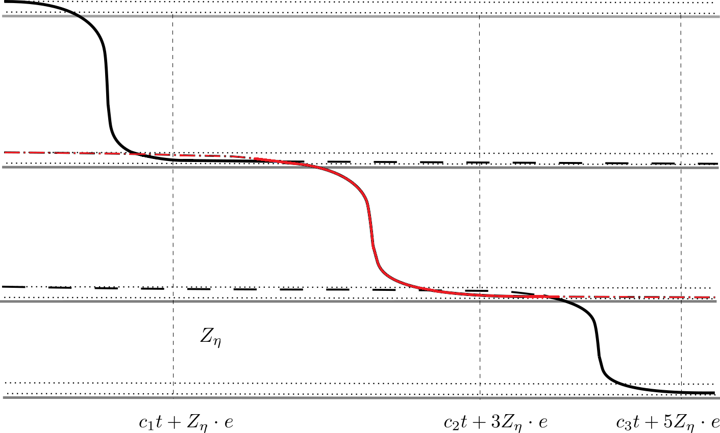
Figure 1: Illustration of the construction of the supersolution $\overline{u}^{\eta}$ at a fixed time $t$. The horizontal axis represents the variable $x\cdot e$. The horizontal straight lines are the steady states (including three platforms). The solid line is $\overline{u}^{\eta}$, which is taken in each interval as a minimum between two perturbed travelling fronts (drawn in either dashed or dash-dotted lines).

It also entails that, for any $t\geq 0$ and $x\in\mathbb{R}^{N}$, there exists $k\in\{1,\dots,K\}$ such that $\overline{u}^{\eta}$ touches $\widetilde{u}^{\eta}_{k}$ from below at $(t,x)$, in the sense that

$$0=\big{(}\overline{u}^{\eta}-\widetilde{u}^{\eta}_{k}\big{)}(t,x)=\max_{|y-x|+|c_{k}(s-t)|<1}\big{(}\overline{u}^{\eta}-\widetilde{u}^{\eta}_{k}\big{)}(s,y).$$ (3.9)

This property implies that $\overline{u}^{\eta}$ acts as a supersolution in the region where the corresponding $\widetilde{u}^{\eta}_{k}$ is, hence $\overline{u}^{\eta}$ will be a generalised supersolution whenever sufficiently close to the steady states $q_{k}$.

Step 2. The time-sliding method.
For $\eta<\bar{\eta}$, let $\overline{u}^{\eta}$ be the function constructed above. Call

$$u(t,x):=U^{\prime}_{K^{\prime}}(x,x\cdot e-c_{K^{\prime}}^{\prime}t).$$ (3.10)

On the one hand, one has that $u(t,x)<q^{\prime}_{K^{\prime}-1}\leq\overline{p}$ and moreover $u(t,x)\to\underline{p}$ as $x\cdot e\to+\infty$, locally uniformly in $t\in\mathbb{R}$. We point out that $c^{\prime}_{K^{\prime}}$ may a priori be zero, and that we made use of Proposition 3.5 here. On the other hand, the function $\overline{u}^{\eta}$ satisfies $\overline{u}^{\eta}\geq\underline{p}+\eta\min\varphi_{K}$ and $\overline{u}^{\eta}(t,x)\to\overline{p}+3\eta\varphi_{0}$ as $x\cdot e\to-\infty$, locally uniformly with respect to $t\geq 0$. As a consequence, we can find $Z\in\mathbb{Z}^{N}$ such that $Z\cdot e$ is large enough to have

$$\forall t\in[0,1],\quad\inf_{x\in\mathbb{R}^{N}}\big{(}\overline{u}^{\eta}(t,x)-u(t,x+Z)\big{)}>0.$$

Then, up to replacing $u(t,x)$ with $u(t,x+Z)$, which is still a pulsating travelling front of (1.1), we can assume without loss of generality that $\inf_{x\in\mathbb{R}^{N}}(\overline{u}^{\eta}(t,x)-u(t,x))>0$ for all $t\in[0,1]$.

We now distinguish two cases.

Case 1: $\overline{u}^{\eta}(t_{0},x_{0})\leq u(t_{0},x_{0})$ for some $t_{0}>0$ and $x_{0}\in\mathbb{R}^{N}$.
We can define the following real number:

$$t_{\eta}:=\inf\big{\{}t\geq 0\ :\ \inf_{x\in\mathbb{R}^{N}}\big{(}\overline{u}^{\eta}-u\big{)}(t,x)=0\big{\}}.$$

We know that $t_{\eta}>1$. There holds that

$$\forall t\in[0,t_{\eta}),\ \inf_{x\in\mathbb{R}^{N}}\big{(}\overline{u}^{\eta}-u\big{)}(t,x)>0,$$

and there exists a sequence $(x_{n})_{n\in\mathbb{N}}$ in $\mathbb{R}^{N}$ such that

$$\lim_{n\to+\infty}\big{(}\overline{u}^{\eta}-u\big{)}(t_{\eta},x_{n})=0.$$

Up to extraction of a subsequence, there exists $k\in\{1,\dots,K\}$ (depending on $\eta$) such that (3.9) holds at the points $(t_{\eta},x_{n})$. We deduce that

$$\lim_{n\to+\infty}\big{(}\widetilde{u}_{k}^{\eta}-u\big{)}(t_{\eta},x_{n})=0,$$ (3.11)

and

$$\forall s\in[0,t_{\eta}),\quad\inf_{|y-x_{n}|+|c_{k}(s-t_{\eta})|<1}\big{(}\widetilde{u}_{k}^{\eta}-u\big{)}(s,y)>0.$$ (3.12)

Let $(h_{n})_{n\in\mathbb{N}}$ be a sequence of points in $\mathbb{Z}^{N}$ such that $(\xi_{n}:=x_{n}-h_{n})_{n\in\mathbb{N}}$ is bounded. By parabolic estimates, the functions $u(\cdot,h_{n}+\cdot)$, $\widetilde{u}_{k}^{\eta}(\cdot,h_{n}+\cdot)$ converge locally uniformly as $n\to+\infty$ (up to subsequences) towards two functions $v$ and $v_{k}^{\eta}$, the former being a solution to (1.1) and the latter being a strict supersolution whenever $v_{k}^{\eta}>q_{k-1}-\bar{\eta}$ or $v_{k}^{\eta}<q_{k}+\bar{\eta}$, thanks to Lemma 3.6. Moreover, calling $\xi$ the limit of (a subsequence of) $(\xi_{n})_{n\in\mathbb{N}}$, we obtain from (3.11) and (3.12) that

$$\min_{|y-\xi|+|c_{k}(s-t_{\eta})|<1}\big{(}v_{k}^{\eta}-v\big{)}(s,y)=\big{(}v_{k}^{\eta}-v\big{)}(t_{\eta},\xi)=0.$$

We necessarily have that

$$q_{k}(\xi)+\bar{\eta}\leq v_{k}^{\eta}(t_{\eta},\xi)\leq q_{k-1}(\xi)-\bar{\eta},$$

because otherwise we would get a contradiction with the parabolic comparison principle. We infer that, for $n$ large enough,

$$q_{k}(x_{n})+\frac{\bar{\eta}}{2}\leq\widetilde{u}_{k}^{\eta}(t_{\eta},x_{n})\leq q_{k-1}(x_{n})-\frac{\bar{\eta}}{2}.$$ (3.13)

Case 2: $\overline{u}^{\eta}(t,x)>u(t,x)$ for all $t\geq 0$, $x\in\mathbb{R}^{N}$.
We will reduce to a case similar to the previous one, but in the limit as $t\to+\infty$. First of all, we restrict ourselves to $\eta<\min\{\bar{\eta},\hat{\eta}\}$, where $\hat{\eta}>0$ is such that

$$q_{K}+2\hat{\eta}=\underline{p}+2\hat{\eta}<q^{\prime}_{K^{\prime}-1}.$$

We claim that then necessarily $c^{\prime}_{K^{\prime}}=c_{K}$. Suppose by contradiction that this is not the case. Since by hypothesis $c^{\prime}_{K^{\prime}}\geq c_{K}$, this means that $c^{\prime}_{K^{\prime}}>c_{K}$. But then, taking $c_{K}<c<c^{\prime}_{K^{\prime}}$, we infer from the definition (3.10) of $u$ and that of $\overline{u}^{\eta}$, as well as the choice of $\hat{\eta}$, that

$$\limsup_{t\to+\infty}(\overline{u}^{\eta}-u)(t,cte)\leq\limsup_{t\to+\infty}(q_{K}+\eta\varphi_{K}-q^{\prime}_{K^{\prime}-1})(cte)\leq-\hat{\eta}<0,$$

which is excluded in the present case. This shows that $c_{K}=c^{\prime}_{K^{\prime}}$ in this case, whence, by the hypothesis of the proposition, $c_{K}=c^{\prime}_{K^{\prime}}\neq 0$.

We now translate $u$ in the $t$ variable. Namely, for $\tau\in\mathbb{R}$, we define

$$D(\tau):=\liminf_{t\to+\infty}\Big{(}\inf_{x\in\mathbb{R}^{N}}(\overline{u}^{\eta}(t,x)-u(\tau+t,x)\Big{)}.$$

Since $\overline{u}^{\eta}>u$ on $[0,+\infty)\times\mathbb{R}^{N}$, we have $D(0)\geq 0$. We claim that $D(\tau)\leq 0$ for some $\tau\in\mathbb{R}$. To see this, we observe that, for $t\geq 0$ and $x_{t}$ such that $x_{t}\cdot e=c_{K}t+(2K-1)Z_{\eta}\cdot e$, it holds $\overline{u}^{\eta}(t,x_{t})=\widetilde{u}^{\eta}_{K}(t,x_{t})$ and moreover $(x_{t}-2(K-1)Z_{\eta})\cdot e-c_{K}t=Z_{\eta}\cdot e\geq z_{\eta}$, whence, by (3.8),

$$\overline{u}^{\eta}(t,x_{t})=\widetilde{u}^{\eta}_{K}(t,x_{t})<q_{K}(x_{t})+2\eta\varphi_{K}(x_{t})<q^{\prime}_{K^{\prime}-1}(x_{t}),$$

whereas, recalling (3.10),

$$u(\tau+t,x_{t})=U^{\prime}_{K^{\prime}}(x_{t},-c^{\prime}_{K^{\prime}}\tau+(2K-1)Z_{\eta}).$$

Therefore, if $c^{\prime}_{K^{\prime}}\tau>0$ is sufficiently large, one has $\overline{u}^{\eta}(t,x_{t})<u(\tau+t,x_{t})$ for all $t\geq 0$. For such values of $\tau$ we thereby have $D(\tau)\leq 0$. Since the function $D$ is continuous (because $u$ is uniformly continuous in $t$) there exists then $\tau^{*}\in\mathbb{R}$ such that $D(\tau^{*})=0$.

Let $(t_{n})_{n\in\mathbb{N}}$ be a sequence diverging to $+\infty$, and $(x_{n})_{n\in\mathbb{N}}$ be a sequence in $\mathbb{R}^{N}$ such that

$$\lim_{n\to\infty}\big{(}\overline{u}^{\eta}(t_{n},x_{n})-u(\tau^{*}+t_{n},x_{n})\big{)}=0.$$

We can find $k\in\{1,\dots,K\}$ (depending on $\eta$) such that (3.9) holds at $(t,x)=(t_{n},x_{n})$ for all $n\in\mathbb{N}$, up to extraction of a subsequence, hence

$$\lim_{n\to+\infty}\big{(}\widetilde{u}_{k}^{\eta}(t_{n},x_{n})-u(\tau^{*}+t_{n},x_{n})\big{)}=0,$$ (3.14)

and in addition, using $D(\tau^{*})=0$,

$$\liminf_{n\to+\infty}\bigg{(}\inf_{|y-x_{n}|+|c_{k}(s-t_{n})|<1}\big{(}\widetilde{u}_{k}^{\eta}(s,y)-u(\tau^{*}+s,y)\big{)}\bigg{)}\geq 0.$$ (3.15)

As in the previous case, we consider a sequence $(h_{n})_{n\in\mathbb{N}}$ of points on $\mathbb{Z}^{N}$ such that $(x_{n}-h_{n})_{n\in\mathbb{N}}$ is bounded. By parabolic estimates, the functions $u(\tau^{*}+t_{n}+\cdot,h_{n}+\cdot)$, $\widetilde{u}_{k}^{\eta}(t_{n}+\cdot,h_{n}+\cdot)$ converge locally uniformly, as $n\to+\infty$ (up to subsequences), towards two functions $v$ and $v_{k}^{\eta}$. The former is still a solution to (1.1), whereas the latter, owing to Lemma 3.6, is a (strict) supersolution whenever $v_{k}^{\eta}>q_{k-1}-\bar{\eta}$ or $v_{k}^{\eta}<q_{k}+\bar{\eta}$. Moreover, (3.14) and (3.15) imply that $v$ touches $v_{k}^{\eta}$ from below at $(0,\xi)$, where $\xi=\lim_{n\to+\infty}(x_{n}-h_{n})$. The parabolic strong maximum principle then yields

$$q_{k}(\xi)+\bar{\eta}\leq v_{k}^{\eta}(0,\xi)\leq q_{k-1}(\xi)-\bar{\eta},$$

whence, for large enough $n$,

$$q_{k}(x_{n})+\frac{\bar{\eta}}{2}\leq\widetilde{u}_{k}^{\eta}(t_{n},x_{n})\leq q_{k-1}(x_{n})-\frac{\bar{\eta}}{2}.$$ (3.16)

Step 3. Conclusion.
In any case, for $0<\eta<\min\{\bar{\eta},\hat{\eta}\}$, by either (3.11)-(3.12) or (3.14)-(3.15), we can find $k_{\eta}\in\{1,\dots K\}$, $t_{\eta}>1$, $\tau_{\eta}\in\mathbb{R}$ and $x_{\eta}\in\mathbb{R}^{N}$ such that the following hold:

$$\widetilde{u}_{k_{\eta}}^{\eta}(t_{\eta},x_{\eta})-u(\tau_{\eta}+t_{\eta},x_{\eta})<\eta,$$ (3.17)

$$\forall s\in[0,t_{\eta}),\quad\inf_{|y-x_{\eta}|+|c_{k_{\eta}}(s-t_{\eta})|<1}\big{(}\widetilde{u}_{k_{\eta}}^{\eta}(s,y)-u(\tau_{\eta}+s,y)\big{)}>-\eta,$$ (3.18)

and in addition, by (3.13) or (3.16),

$$q_{k_{\eta}}(x_{\eta})+\frac{\bar{\eta}}{2}\leq\widetilde{u}_{k_{\eta}}^{\eta}(t_{\eta},x_{\eta})\leq q_{{k_{\eta}}-1}(x_{\eta})-\frac{\bar{\eta}}{2}.$$ (3.19)

We can find a sequence $\eta\to 0^{+}$ along which all these properties are fulfilled with the same integer $k_{\eta}=k$. Observe that the associated sequence

$$x_{\eta}\cdot e-2(k-1)Z_{\eta}\cdot e-c_{k}t_{\eta}$$

remains bounded as $\eta\to 0^{+}$, owing to (3.8) and (3.19).

Let $(h_{\eta})_{\eta}$ in $\mathbb{Z}^{N}$ be such that $(\xi_{\eta}:=x_{\eta}-h_{\eta})_{\eta}$ is bounded, hence $(h_{\eta}\cdot e-2(k-1)Z_{\eta}\cdot e-c_{k}t_{\eta})_{\eta}$ is bounded too. Call $\xi$ and $\zeta$ their respective limits as $\eta\to 0^{+}$ (up to subsequences). We have that, as (a sequence of) $\eta\to 0^{+}$,

$$\widetilde{u}_{k}^{\eta}(t_{\eta}+t,h_{\eta}+x)\to U_{k}(x,x\cdot e-c_{k}t+\zeta),\qquad u(\tau_{\eta}+t_{\eta}+t,h_{\eta}+x)\to U^{\prime}_{K^{\prime}}(x,x\cdot e-c^{\prime}_{K^{\prime}}t+\zeta^{\prime}),$$

locally uniformly in $(t,x)$, with

$$\zeta^{\prime}:=\lim_{\eta\to 0^{+}}\big{(}h_{\eta}\cdot e-c^{\prime}_{K^{\prime}}(\tau_{\eta}+t_{\eta})\big{)}\in\mathbb{R}\cup\{\pm\infty\}.$$

For clarity we point out that, when $\zeta^{\prime}=\pm\infty$, then $U^{\prime}_{K^{\prime}}(x,x.e-c^{\prime}_{K^{\prime}}t+\zeta^{\prime})$ should be understood as one of the periodic states $q^{\prime}_{K^{\prime}}$ (i.e. $0$) or $q^{\prime}_{K^{\prime}-1}$.

Passing to the limit $\eta\to 0$ in (3.17)-(3.18) yields

$$U_{k}(\xi,\xi\cdot e+\zeta)-U^{\prime}_{K^{\prime}}(\xi,\xi\cdot e+\zeta^{\prime})\leq 0,$$

$$\forall s\in(-1,0),\quad\inf_{|y-\xi|+|c_{k}s|<1}\big{(}U_{k}(y,y\cdot e-c_{k}s+\zeta)-U^{\prime}_{K^{\prime}}(y,y\cdot e-c^{\prime}_{K^{\prime}}s+\zeta^{\prime})\big{)}\geq 0.$$

Since $U_{k}(x,x\cdot e-c_{k}t+\zeta)$, $U^{\prime}_{K^{\prime}}(x,x\cdot e-c^{\prime}_{K^{\prime}}t+\zeta^{\prime})$ are solutions of (1.1), the strong maximum principle and the unique continuation property (see, e.g., Section 4 in [17]) imply that

$$\forall x\in\mathbb{R}^{N},\ t\in\mathbb{R},\quad U_{k}(x,x\cdot e-c_{k}t+\zeta)=U^{\prime}_{K^{\prime}}(x,x\cdot e-c^{\prime}_{K^{\prime}}t+\zeta^{\prime}).$$

From this, and the properties of pulsating travelling fronts, one readily deduces that $c_{k}=c_{K^{\prime}}^{\prime}$, that $U^{\prime}_{K^{\prime}}$ is necessarily the “bottom” of the terrace $\mathcal{T}$ too, i.e. $k=K$, and that $U_{K}$ and $U^{\prime}_{K^{\prime}}$ coincide up to translation (on the set $(x,x.e)$, $x\in\mathbb{R}^{N}$, in the case $c_{K^{\prime}}^{\prime}=0$). ∎

The uniqueness of the terrace now follows by recursively applying Proposition 3.7.

Proof of Theorem 2.1.

Let $\mathcal{T}$ and $\mathcal{T}^{\prime}$ be two terraces connecting $\overline{p}$ to $0$ in a direction $e\in S^{N-1}$, with the speeds of the former being all non-zero. Proposition 3.7 implies that the lowest profiles of $\mathcal{T}$ and $\mathcal{T}^{\prime}$ coincide, up to a translation. Dropping this lowest profile from both $\mathcal{T}$ and $\mathcal{T}^{\prime}$, we obtain two terraces connecting $\overline{p}$ to the same state $\underline{p}>0$, which by Proposition 3.3 is thereby stable. We can then apply Proposition 3.7 to these new terraces and find that they also share the same lowest profile (up to shift). Iterating we eventually infer that $\mathcal{T}$ and $\mathcal{T}^{\prime}$ coincide up to shift of their profiles. ∎

Remark 3.1.

Notice that the argument in this section still partly applies when the terrace $\mathcal{T}$ has some fronts with zero speeds. Indeed, assume that the lowest (hence fastest) fronts of $\mathcal{T}$ have positive speeds. Then the previous induction still works in the same way, until one reaches a front of $\mathcal{T}$ with zero speed. Putting this with a symmetrical argument for the uppermost fronts, one would find that any other terrace must include all the fronts of $\mathcal{T}$ whose speeds are not zero. However, terraces may still differ in and between the platforms of $\mathcal{T}$ connected by travelling fronts with zero speed (see [12, Section 6] for related comments in the one dimensional case).

3.3 A procedure for the determination of the terrace

Theorem 2.1 guarantees the uniqueness of the terrace, in any given direction. We now present a procedure for determining such a terrace, and in particular its platforms, i.e. the states that are “selected” by the terrace. This is based on an iterative argument involving the speeds of the fronts connecting the steady states. We also refer to [12, Section 6] for some examples in the one dimensional case.

We exhibit the procedure in the case where the linearly stable, periodic steady states provided by Assumption 1 are ordered, i.e. they are given by

$$p_{0}>p_{1}>\cdots>p_{M},$$

for some $M\geq 1$. For any $k\in\{1,\dots,M\}$, the equation is bistable between $p_{k}$ and $p_{k-1}$, hence the propagating terrace provided by Theorem 1.3 in any given direction $e\in S^{N-1}$ reduces to a pulsating travelling front connecting $p_{k-1}$ to $p_{k}$; let $U_{k}$ be its profile and $c_{k}$ be its speed. We point out that the latter is unique by Theorem 2.1 (even when $c_{k}=0$). One of the following situations occurs:

1. the family $(c_{k})_{1\leq k\leq K}$ is monotonically non-decreasing, i.e.

   $$c_{k-1}\leq c_{k}\quad\text{ for all }\;k\in\{2,\dots,M\};$$

2. there exists $J\in\{2,\dots,M\}$ such that

   $$c_{J-1}>c_{J}.$$

In the case $(i)$, the terrace $\mathcal{T}$ in the direction $e$ is composed by the whole family of front profiles $(U_{k})_{k=1,\dots,M}$ (and the corresponding platforms). In the case $(ii)$, it follows from Theorem 1.3 that the terrace connecting $p_{J-2}$ to $p_{J}$ is composed by a single pulsating travelling front, with a profile $\widetilde{U}_{J}$ (and it follows from our Theorem 2.2 that $\widetilde{c}_{J}\in[c_{J},c_{J-1}]$). One is therefore left with the family of stacked front profiles

$$U_{1},\dots,U_{J-2},\widetilde{U}_{J},U_{J+1},\dots,U_{M},$$

and thus may repeat the previous argument. Since the number of fronts is reduced by one, after at most $M$ iterations one ends up in the case $(i)$, that is, one has constructed the terrace $\mathcal{T}$.

One should notice that the order in which one picks the pair of fronts to be “merged together” does not matter, due to the fact that the speed of the resulting front is between the speeds of the two merged fronts. The general principle is that lowest fronts can only speed down a given front, while highest fronts can only speed it up.

3.4 Spreading speeds for planar-like initial data

In this section, we prove Theorem 2.2, i.e. that the propagating terrace determines the spreading speeds for planar-like initial data. We will rely on a similar construction as in the proof of Lemma 3.6, but this time we will need the function to be a supersolution everywhere.

We place ourselves in the hypotheses of Theorem 2.2, that is, under Assumption 1 and the existence of a propagating terrace $\mathcal{T}=((q_{k})_{0\leq k\leq K},(U_{k})_{1\leq k\leq K})$ in the direction $e\in S^{N-1}$ whose speeds are non-zero. Then Theorem 2.1 guarantees that $\mathcal{T}$ is unique (up to shifts), and in particular it coincides with the terrace given by Theorem 1.3. The condition (2.1) of the speeds being non-zero allows one to strengthen the conclusion of Lemma 3.6 by getting a function which is everywhere a supersolution, at the price of slightly increasing its speed. For its construction, we again make use of a smooth and nondecreasing function $\chi$ satisfying (3.4), as well as of the periodic principal eigenfunctions $\varphi_{k}$ of the problems (3.1) with $p=q_{k}$, that we normalise by ${\max\varphi_{k}=1}$.

Lemma 3.8.

For $k\in\{1,\dots,K\}$ and $\varepsilon>0$, call

$$\overline{\psi}_{k}(t,x):=(1-\chi(x\cdot e-(c_{k}+\varepsilon)t))\varphi_{k-1}(x)+\chi(x\cdot e-(c_{k}+\varepsilon)t)\varphi_{k}(x).$$

Then there exists $\delta_{k}>0$ such that, for all $\eta\in[0,\delta_{k}]$, the function

$$\overline{u}_{k}(t,x):=U_{k}(x,x\cdot e-(c_{k}+\varepsilon)t)+\eta\overline{\psi}_{k}(t,x)$$

is a supersolution of (1.1).

Proof.

Consider the quantity $\delta>0$ given by Lemma 3.1 in the case $p=q_{k}$. We can choose $Z\geq 1$ large enough so that the following properties hold:

$$\forall x\in\mathbb{R}^{N},\ \forall z\leq-Z,\qquad|U_{k}(x,z)-q_{k-1}(x)|\leq\delta,$$

$$\forall x\in\mathbb{R}^{N},\ \forall z\geq Z,\qquad|U_{k}(x,z)-q_{k}(x)|\leq\delta.$$

Observe that $U_{k}(x,x\cdot e-(c_{k}+\varepsilon)t)$ is a supersolution of (1.1) because $U_{k}(x,z)$ is nonincreasing with respect to $z$, thanks to Theorem 1.3. Consider the function $\overline{u}_{k}$ defined in the statement of the lemma. On one hand, since

$$\overline{u}_{k}(t,x)=\begin{cases}U_{k}(x,x\cdot e-(c_{k}+\varepsilon)t)+\eta\varphi_{k-1}(x)&\text{if }\;x\cdot e-(c_{k}+\varepsilon)t<-Z,\\ U_{k}(x,x\cdot e-(c_{k}+\varepsilon)t)+\eta\varphi_{k}(x)&\text{if }\;x\cdot e-(c_{k}+\varepsilon)t>Z\,,\end{cases}$$

Lemma 3.1 implies that $\overline{u}_{k}(t,x)$ is a supersolution of (1.1) in the region $t\geq 0$, $|x\cdot e-(c_{k}+\varepsilon)t|>Z$, for any choice of $\eta\in[0,\delta]$. On the other hand, differentiating in time the equation (1.1) satisfied by $u_{k}(t,x):=U_{k}(x,x\cdot e-c_{k}t)$, one gets a linear equation for $\partial_{t}u_{k}(t,x)=-c_{k}\partial_{z}U_{k}$, which we know is a nonnegative or nonpositive function, according to the sign of the (non-zero) speed $c_{k}$. It then follows from the parabolic strong maximum principle that $\partial_{z}U_{k}$ cannot vanish somewhere without being identically equal to $0$, which is impossible since $U(\cdot,-\infty)>U(\cdot+\infty)$. As a consequence, due to the periodicity of $U_{k}$ with respect to its first variable, we get

$$\rho:=\min_{\begin{subarray}{c}x\in\mathbb{R}^{N}\\ |z|\leq Z\end{subarray}}\left[-\partial_{z}U_{k}(x,z)\right]>0.$$

We compute

$$\partial_{t}\overline{u}_{k}-\operatorname{div}(A(x)\nabla\overline{u}_{k})-f(x,\overline{u}_{k})\geq\eta\big{(}\partial_{t}\overline{\psi}_{k}-\operatorname{div}(A(x)\nabla\overline{\psi}_{k})\big{)}-\varepsilon\partial_{z}U_{k}+f(x,U_{k})-f(x,\overline{u}_{k}),$$

where $U_{k}$, $\partial_{z}U_{k}$ are evaluated at $(x,x\cdot e-(c_{k}+\varepsilon)t)$. The last two terms above are controlled by

$$|f(x,U_{k})-f(x,\overline{u}_{k})|\leq\eta\|\partial_{u}f\|_{L^{\infty}(\mathbb{R}^{N}\times[-\eta,\|\overline{p}\|_{\infty}+\eta])}.$$

We then have, for $t\geq 0$ and $|x\cdot e-(c_{k}+\varepsilon)t|\leq Z$,

$$\partial_{t}\overline{u}_{k}-\operatorname{div}(A(x)\nabla\overline{u}_{k})-f(x,\overline{u}_{k})\geq\varepsilon\rho-M_{k}\eta-\eta\|\partial_{u}f\|_{L^{\infty}(\mathbb{R}^{N}\times[-\eta,\|\overline{p}\|_{\infty}+\eta])},$$

with $M_{k}$ only depending on $A$ and the function $\overline{\psi}_{k}$, which in turn depends on $\chi,\varphi_{k-1},\varphi_{k}$. As a consequence, for $\eta$ sufficiently small, the function $\overline{u}_{k}$ is a supersolution of (1.1). ∎

Remark 3.2.

Several comments are in order.

1. We point out that analogous versions of Lemmas 3.6, 3.8 hold true for subsolutions, just obtained as $\overline{p}(x)-\overline{u}_{k}^{\eta}(t,x)$ and $\overline{p}(x)-\overline{u}_{k}(t,x)$ respectively (which propagate in the direction $-e$ with speed $-c_{k}$ and $-(c_{k}+\varepsilon)$ respectively).

2. For the function $\overline{u}_{k}$ of Lemma 3.8 to be a supersolution, the strict inequality $\partial_{z}U_{k}<0$ is necessary, which requires $c_{k}\neq 0$. In the case $c_{k}=0$ it is even unclear whether $z\mapsto U(x,z)$ is continuous, as we discussed in [13, Remark 3]. Actually, using $\partial_{z}U_{k}<0$, one could have constructed a finer supersolution, namely, a function approaching exponentially $U_{k}(x,x\cdot e-(c_{k}+\varepsilon)t)$ as $t\to+\infty$.

3. Using $\overline{u}_{k}$ with $k=1$, one can derive the sharp upper bound for the uppermost spreading speed, but not for lower speeds. To get those, we will “glue” together the supersolutions $\overline{u}_{k}$. This will require that the speeds at which they move are strictly ordered with respect to $k$. For this purpose, we will perturb the speeds $(c_{k})_{k}$ by an increasing family $(\varepsilon_{k})_{k}$. In the case where the $(c_{k})_{k}$ are already strictly ordered, one may replace the perturbation terms $\varepsilon_{k}t$ by some exponentially decaying term $C(1-e^{-\gamma t})$ with some well chosen constants $C,\gamma$, as in the classical “sandwich argument” of Fife and Mc Leod [10]. Combined with the above considerations 1 and 2, this would lead to a slightly more accurate result under this additional assumption (see also part $2$ of Remark 2.1).

We can now prove the convergence of solutions with “planar-like” initial data to the terrace, far from the regions $x\cdot e=c_{k}t$ where the interfaces are located.

Proof of Theorem 2.2.

We only derive the upper estimate for the spreading speed. The lower estimate follows by considering the initial datum $\overline{p}-u_{0}$ (which is still planar-like but in the opposite direction $-e$) and the corresponding solution of (1.1) with $f(x,u)$ replaced by $f(x,\overline{p}(x)-u)$ (which still satisfies Assumption 1).

Consider an increasing finite sequence of strictly positive numbers $(\varepsilon_{k})_{1\leq k\leq K}$. We have

$$\forall k\in\{1,\dots,K-1\},\qquad c_{k}+\varepsilon_{k}<c_{k+1}+\varepsilon_{k+1}.$$

Next, set $\delta^{\prime}:=\min\{\delta_{1},\dots,\delta_{K}\}$, where the $\delta_{k}$ are given by Lemma 3.8. Call also

$$\delta^{\prime\prime}:=\min_{1\leq k\leq K-1}\Big{(}\min(q_{k}-q_{k+1})\Big{)},$$

which is positive because the platforms of a terrace are strictly ordered. Then consider an increasing finite sequence $(\eta_{k})_{1\leq k\leq K}$ in $(0,\min\{\delta^{\prime},\delta^{\prime\prime}\})$. Finally, for $k\in\{1,\dots,K\}$, consider the function $\overline{u}_{k}$ given by Lemma 3.8, with $\eta=\eta_{k}$. It holds that

$$\overline{u}_{k}(t,x)-q_{k}(x)-\eta_{k}\varphi_{k}(x)\to 0\quad\text{ as }\;x\cdot e-(c_{k}+\varepsilon_{k})t\to+\infty,$$

while

$$\overline{u}_{k+1}(t,x)-q_{k}(x)-\eta_{k+1}\varphi_{k}(x)\to 0\quad\text{ as }\;x\cdot e-(c_{k+1}+\varepsilon_{k+1})t\to-\infty.$$

Take $\widetilde{c}_{1},\dots,\widetilde{c}_{K-1}\in\mathbb{R}$ such that

$$\forall k\in\{1,\dots,K-1\},\qquad c_{k}+\varepsilon_{k}<\widetilde{c}_{k}<c_{k+1}+\varepsilon_{k+1}.$$

Since $\eta_{k+1}>\eta_{k}$, from the above limits we infer the existence of some large enough $t_{k}>0$ such that

$$\forall t\geq t_{k}\ \;\text{and}\;\ x\cdot e=\widetilde{c}_{k}t,\qquad\overline{u}_{k}(t,x)<\overline{u}_{k+1}(t,x),$$

and in addition, using that $\eta_{k+1}\varphi_{k+1}\leq\eta_{k+1}<\min(q_{k}-q_{k+1})$, such that

$$\forall t\geq t_{k}\ \;\text{and}\;\ x\cdot e\geq\widetilde{c}_{k+1}t,\qquad\overline{u}_{k}(t,x)>\overline{u}_{k+1}(t,x).$$

It follows that the function $\overline{u}$ defined by

$$\overline{u}(t,x):=\begin{cases}\overline{u}_{1}(t,x)&\text{if }x\cdot e<\widetilde{c}_{1}t,\\[5.0pt] \min\big{\{}\overline{u}_{k}(t,x),\overline{u}_{k+1}(t,x)\big{\}}\ \quad&\text{if }\;\widetilde{c}_{k}t\leq x\cdot e<\widetilde{c}_{k+1}t\\ &\text{for some $k\in\{1,\dots,K-1\}$,}\\[5.0pt] \overline{u}_{K}(t,x)&\text{if }x\cdot e\geq\widetilde{c}_{K}t,\end{cases}$$

is continuous for $t\geq T:=\max\{t_{1},\dots,t_{K}\}$. The shape of $\overline{u}$ is similar to the one of $\overline{u}^{\eta}$ in the proof of Proposition 3.7, see Figure 1 for an illustration.

By Lemma 3.8, the function $\overline{u}$ is a generalised supersolution of (1.1) for $t>T$ (being essentially the minimum of supersolutions). We also note that

$$\forall t\geq t_{k}\ \;\text{and}\;\ x\cdot e\geq\widetilde{c}_{k}t,\qquad\overline{u}(t,x)\leq\overline{u}_{k}(t,x).$$

We deduce that, for all $k\in\{1,\dots,K\}$,

$$\limsup_{t\to+\infty}\Big{(}\sup_{x\cdot e\geq\widetilde{c}_{k}t}\big{(}\overline{u}(t,x)-q_{k}(x)\big{)}\Big{)}\leq\limsup_{t\to+\infty}\Big{(}\sup_{x\cdot e\geq\widetilde{c}_{k}t}\big{(}\overline{u}_{k}(t,x)-q_{k}(x)\big{)}\Big{)}\leq\eta_{k}.$$ (3.20)

One further sees that

$$\liminf_{x\cdot e\to-\infty}\big{(}\overline{u}(T,x)-\overline{p}(x)\big{)}>0,$$

$$\inf_{x\in\mathbb{R}^{N}}\overline{u}(T,x)>0.$$

On the other hand, according to the assumptions of the theorem, the initial datum $u_{0}$ satisfies that $0\leq u_{0}\leq\overline{p}$, and furthermore $u_{0}(x)<\eta$ for $x\cdot e$ sufficiently large, with $\eta$ belonging to the basin of attraction of $0$. One deduces that the solution $u$ of (1.1) satisfies, on the one hand, $u(t,x)\leq\overline{p}(x)$ for all $t\geq 0$, $x\in\mathbb{R}^{N}$, by comparison, and on the other hand, by passing to the limit as $x\cdot e\to+\infty$ and using parabolic estimates, that

$$\lim_{t\to+\infty}\Big{(}\,\limsup_{x\cdot e\to+\infty}u(t,x)\Big{)}=0.$$

Therefore, we can find $T^{\prime}>0$ and $j\in\mathbb{Z}^{N}$ with $j\cdot e$ large enough in such a way that

$$\forall x\in\mathbb{R}^{N},\quad u(T^{\prime},x)\leq\overline{u}(T,x-j).$$

Applying a comparison principle we find that $u(t,x)\leq\overline{u}(t+T-T^{\prime},x-j)$ for $t\geq T^{\prime}$ and $x\in\mathbb{R}^{N}$. In particular, (3.20) yields

$$\forall k\in\{1,\dots,K\},\quad\limsup_{t\to+\infty}\Big{(}\sup_{(x-j)\cdot e\geq\widetilde{c}_{k}(t+T-T^{\prime})}\big{(}u(t,x)-q_{k}(x)\big{)}\Big{)}\leq\eta_{k}.$$

Recall that $\widetilde{c}_{k}$ was arbitrarily taken in $(c_{k}+\varepsilon_{k},c_{k+1}+\varepsilon_{k+1})$, and that $(\varepsilon_{k})_{1\leq k\leq K}$ was an arbitrary increasing sequence of positive numbers and $(\eta_{k})_{1\leq k\leq K}$ was an arbitrary increasing sequence in $(0,\min\{\delta^{\prime},\delta^{\prime\prime}\})$. This shows the second limit in the statement of the theorem. ∎

4 The compactly supported case under Assumption 2

This section is devoted to the proof of Theorem 2.4, but also includes several general results that will be used again later. For a given direction $e\in S^{N-1}$, we will consider a propagating terrace $\mathcal{T}^{e}$ connecting $\overline{p}$ to $0$ in the direction $e$, and, calling $c_{1}(e)$ the speed of its uppermost travelling front, we will assume that

$$c_{1}(e)>0\quad\text{ for all }\;e\in S^{N-1}.$$ (4.1)

Hence, all speeds of $\mathcal{T}^{e}$ are positive and thus by Theorem 2.1, $\mathcal{T}^{e}$ is the unique terrace (up to shifts) in the direction $e$. From now on, when we refer to condition (4.1), it will always be understood that $c_{1}(e)$ is associated with the (a fortiori unique) terrace $\mathcal{T}^{e}$.

We start with a preliminary result about the lower semi-continuity of the mapping $e\mapsto c_{1}(e)$. The analogue of this result in the bistable case is given in [20, Proposition 2.5], see also [14].

Lemma 4.1.

Under Assumption 1 and (4.1), the mapping $e\mapsto c_{1}(e)$ is bounded and lower semi-continuous on $S^{N-1}$, hence in particular

$$\inf_{e\in S^{N-1}}c_{1}(e)>0.$$

Proof.

Let us start with the boundedness of $c_{1}$. This is a standard fact, that we show here for the sake of completeness. First, due to the $C^{1}$ regularity and spatial periodicity of $f$, there exists $C>0$ such that

$$\forall x\in\mathbb{R^{N}},\ u\in[0,\max\overline{p}],\quad f(x,u)\leq Cu.$$

Then, a direct computation shows that there exists $\overline{c}$ large enough, depending on $A$ and $C$, such that the function

$$\overline{u}(t,x):=\min\left\{\overline{p}(x),e^{-(x\cdot e-\overline{c}t)}\right\}$$

is a supersolution of (1.1), for any $e\in S^{N-1}$. Applying our Theorem 2.2 on the planar case to the initial datum $\overline{u}(0,x)$, we infer by comparison that $c_{1}(e)\leq\overline{c}$. The speed $c_{1}$ being also positive by (4.1), the claimed boundedness follows.

Now fix $e\in S^{N-1}$ and consider any sequence $(e_{n})_{n\in\mathbb{N}}$ in $S^{N-1}$ converging to $e$. From the boundedness, up to extraction of a subsequence, $(c_{1}(e_{n}))_{n\in\mathbb{N}}$ admits a limit $c\in[0,+\infty)$. We need to show that $c\geq c_{1}(e)$.

Let $U^{e}$ be the uppermost profile of the terrace $\mathcal{T}^{e}$. Then, take $\eta>0$ such that $\overline{p}-\eta$ is in the basin of attraction of $\overline{p}$, cf. Lemma 3.1, and moreover $U^{e}(\cdot,+\infty)<\overline{p}-\eta$. We can then find $\zeta^{e}\in\mathbb{R}$ such that

$$\min_{x\in\mathbb{R}^{N}}(U^{e}(x,\zeta^{e})-\overline{p}(x))=-\frac{\eta}{2}.$$ (4.2)

We then consider the following translations of the pulsating travelling fronts:

$$u_{n}(t,x):=U^{e_{n}}(x,x\cdot e_{n}-c_{1}(e_{n})t+\zeta^{e_{n}}).$$

By parabolic estimates, the $u_{n}$ converge locally uniformly as $n\to+\infty$ (up to subsequences) towards a solution $u(t,x)$ of (1.1). Moreover, on the one hand, for $x\in\mathbb{R}^{N}$ such that $x\cdot e<0$, we have that $x\cdot e_{n}<0$ for $n$ large enough, whence by (4.2),

$$u(0,x)=\lim_{n\to+\infty}U^{e_{n}}(x,x\cdot e_{n}+\zeta^{e_{n}})\geq\overline{p}(x)-\frac{\eta}{2}.$$

It follows from the parabolic comparison principle that

$$u(t,x)\geq\underline{u}(t,x),$$

for any $t\geq 0$ and $x\in\mathbb{R}^{N}$, where $\underline{u}$ is the solution of (1.1) together with

$$\underline{u}(0,x):=\left\{\begin{array}[]{ll}\overline{p}(x)-\frac{\eta}{2}&\mbox{if }x\cdot e<0,\vskip 3.0pt\\ 0&\mbox{if }x\cdot e\geq 0.\end{array}\right.$$

Applying Theorem 2.2 to $\underline{u}$, we deduce that

$$\lim_{t\to+\infty}\sup_{x\cdot e\leq(c_{1}(e)-\varepsilon)t}|u(t,x)-\overline{p}(x)|=0,$$

for any $\varepsilon>0$.

On the other hand, for $t\geq 0$ and $x\in[0,1]^{N}$, it holds by (4.2) that

$$\begin{split}&\min_{x\in[0,1]^{N}}\Big{(}u(t,x+cte+\sqrt{N}e)-\overline{p}(x+cte+\sqrt{N}e)\Big{)}\\ &=\lim_{n\to+\infty}\min_{x\in[0,1]^{N}}\Big{(}U^{e_{n}}(x+c_{1}(e_{n})te_{n}+\sqrt{N}e_{n},x\cdot e_{n}+\sqrt{N}+\zeta^{e_{n}})-\overline{p}(x+cte+\sqrt{N}e)\Big{)}\\ &\leq\lim_{n\to+\infty}\min_{x\in[0,1]^{N}}\Big{(}U^{e_{n}}(x+c_{1}(e_{n})te_{n}+\sqrt{N}e_{n},\zeta^{e_{n}})-\overline{p}(x+c_{1}(e_{n})te_{n}+\sqrt{N}e_{n})\Big{)}\\ &=-\frac{\eta}{2}.\end{split}$$

From these two facts, we eventually infer that $c\geq c_{1}(e)$. ∎

In the following two subsections, we derive an upper and a lower bound on the spreading speed of the level sets, respectively. Whether these bounds coincide in general remains an open problem. We will see that this is the case under Assumption 2, i.e. when all propagating terraces in all directions share the same platforms.

4.1 An upper bound for the spreading speeds

An estimate from above of the spreading speeds of solutions with compactly supported initial data would immediately follow from the comparison with solutions starting from planar-like initial data, whose spreading speeds have been derived in Section 3.4. However, we need an upper estimate which is uniform with respect to the direction, and this requires an additional argument.

More precisely, the next result asserts that the spreading shape is contained in a set, that one may recognize as the upper estimate stated in both Theorems 2.4 and 2.6.

Proposition 4.2.

Under Assumption 1 and (4.1), let $0\leq p<\overline{p}$ be a linearly stable, spatially periodic, steady state of (1.1), and let $W_{c[p]}$ be given by Definitions 2.3 and 2.5. Then, for any solution $u$ emerging from a compactly supported initial datum $0\leq u_{0}\leq\overline{p}$, it holds:

$$\forall\varepsilon>0,\qquad\limsup_{t\to+\infty}\bigg{(}\sup_{x\in\,\mathbb{R}^{N}\setminus(1+\varepsilon)tW_{c[p]}}\big{(}u(t,x)-p(x)\big{)}\bigg{)}\leq 0.$$

Proof.

First recall Definitions 2.3 and 2.5. By (4.1) and Theorem 2.1, for any $e\in S^{N-1}$, there exists a unique (up to shifts) propagating terrace $\mathcal{T}^{e}$ connecting $\overline{p}$ to $0$ in the direction $e$. Then, for $0\leq p<\overline{p}$ a linearly stable, spatially periodic, steady state of (1.1), there exists a unique profile $U$ contained in $\mathcal{T}^{e}$ such that

$$U(\cdot,+\infty)\leq p(\cdot),\qquad\max_{x\in\mathbb{R}^{N}}(U(x,-\infty)-p(x)\big{)}>0.$$

The speed of that front is denoted by $c[p](e)$ and the associated Wulff shape is

$$W_{c[p]}:=\bigcap_{e\in S^{N-1}}\big{\{}x\in\mathbb{R}^{N}\ |\ x\cdot e\leq c[p](e)\big{\}}.$$

By construction, $c[p](e)\geq c_{1}(e)$. Then condition (4.1) together with Lemma 4.1 yield $\inf_{e}c[p](e)>0$. It follows that $W_{c[p]}$ is a non-empty, convex and compact set, which can equivalently be written as

$$W_{c[p]}=\{re\ |\ e\in S^{N-1}\text{\; and \;}0\leq r\leq\overline{w}_{p}(e)\}\quad\text{ with }\ \overline{w}_{p}(e):=\inf_{\begin{subarray}{c}e^{\prime}\in S^{N-1}\\ e^{\prime}\cdot e>0\end{subarray}}\frac{c[p](e^{\prime})}{e\cdot e^{\prime}},$$ (4.3)

and also that the function $e\mapsto\overline{w}_{p}(e)$ is positive and continuous on $S^{N-1}$, c.f. [20, Proposition 2.4].

Next, fix some arbitrary $\varepsilon>0$. Since $u_{0}$ is compactly supported, for any $e\in S^{N-1}$ one can find another initial datum $\widetilde{u}_{0}^{e}$ satisfying the assumptions of Theorem 2.2 and such that $\widetilde{u}_{0}^{e}\geq u_{0}$ in $\mathbb{R}^{N}$. The parabolic comparison principle implies that $u$ is smaller than or equal to the solution emerging from $\widetilde{u}_{0}^{e}$ and therefore we deduce from the upper estimates in Theorem 2.2 that, for any $e\in S^{N-1}$,

$$\limsup_{t\to+\infty}\bigg{(}\sup_{x\cdot e\geq(1+\varepsilon)tc[p](e)}\big{(}u(t,x)-p(x)\big{)}\bigg{)}\leq 0.$$ (4.4)

In order to derive from this the desired estimate, one would need to show that (4.4) holds true uniformly with respect to $e\in S^{N-1}$. We do so by showing that one can reduce to a finite number of directions $e$, up to replacing $\varepsilon$ with $2\varepsilon$. Namely, consider the set

$$(1+2\varepsilon)W_{c[p]}.$$

Its boundary $(1+2\varepsilon)\partial W_{c[p]}$ is a compact set which does not intersect the compact set $(1+\varepsilon)W_{c[p]}$, as it is seen from the expression (4.3), recalling from above that the function $\overline{w}_{p}$ is positive and continuous. This means, by the definition of $W_{c[p]}$, that the family

$$\big{\{}x\in\mathbb{R}^{N}\ |\ x\cdot e>(1+\varepsilon)c[p](e)\big{\}},\quad e\in S^{N-1},$$

is a cover of $(1+2\varepsilon)\partial W_{c[p]}$. We extract from it a finite subcover, that is,

$$(1+2\varepsilon)\partial W_{c[p]}\subset\bigcup_{j=1}^{J}\big{\{}x\in\mathbb{R}^{N}\ |\ x\cdot e_{j}>(1+\varepsilon)c[p](e_{j})\big{\}}.$$

Therefore, since the set

$$\bigcap_{j=1}^{J}\big{\{}x\in\mathbb{R}^{N}\ |\ x\cdot e_{j}\leq(1+\varepsilon)c[p](e_{j})\big{\}}$$

is connected, and intersects $(1+2\varepsilon)W_{c[p]}$ (at least at the origin) but not $(1+2\varepsilon)\partial W_{c[p]}$, we deduce

$$\bigcap_{j=1}^{J}\big{\{}x\in\mathbb{R}^{N}\ |\ x\cdot e_{j}\leq(1+\varepsilon)c[p](e_{j})\big{\}}\subset(1+2\varepsilon)W_{c[p]}.$$

Passing to the complementary on the above inclusion, and using (4.4) on the (finite number of) directions $e_{1},\dots,e_{J}$, one gets

$$\limsup_{t\to+\infty}\bigg{(}\sup_{x\in\,\mathbb{R}^{N}\setminus(1+2\varepsilon)tW_{c[p]}}\big{(}u(t,x)-p(x)\big{)}\bigg{)}\leq 0,$$

which is the desired estimate with $\varepsilon$ replaced by $2\varepsilon$. ∎

4.2 A lower bound for the speed towards $\overline{p}$

Let us turn to the lower bound. We first derive the estimate for the speed of spreading towards the uppermost steady state $\overline{p}$, then we will apply it iteratively to deal with lower states.

Proposition 4.3.

Under Assumption 1 and (4.1), let $u$ be a solution emerging from an initial datum $0\leq u_{0}\leq\overline{p}$ for which (2.4) holds. Then $u$ satisfies

$$\forall\varepsilon\in(0,1),\qquad\liminf_{t\to+\infty}\bigg{(}\inf_{x\in(1-\varepsilon)tW_{c_{1}}}\big{(}u(t,x)-\overline{p}(x)\big{)}\bigg{)}\geq 0,$$ (4.5)

where, consistently with the first item of Definition 2.3,

$$W_{c_{1}}:=\bigcap_{e\in S^{N-1}}\{x\in\mathbb{R}^{N}\ |\ x\cdot e\leq c_{1}(e)\}.$$ (4.6)

We emphasise that Proposition 4.3 only requires Assumption 1 and the positivity of the speeds of the terraces. We remind that the latter ensures that the terrace is unique (up to translation of its profiles) in any given direction, owing to Theorem 2.1. However, Proposition 4.3 only concerns the uppermost state of the terrace. In the sequel we will apply it to terraces connecting some lower positive state to 0, then Assumptions 2 or 3 will be crucial to obtain the sharp estimate on the spreading speeds. For instance, Assumption 2 ensures that for any $1\leq k\leq K-1$, the propagating terrace connecting the platform $q_{k}$ to $0$ is a subset of the original terrace connecting $\overline{p}$ to $0$. Hence the uppermost front of the former is just the $k$-th front of the latter, regardless of the direction.

We prove Proposition 4.3 by combining and refining the geometric arguments employed in [20] and [6] to derive respectively the Freidlin-Gärtner formula and the sufficient condition for invasion (i.e. the local convergence to $\overline{p}$) in the bistable case. These arguments make a link between compactly supported initial data and planar data, hence will allow us to use the spreading speeds for the latter already established in Theorem 2.2.

For later use, we rewrite the set $W_{c_{1}}$ as follows:

$$W_{c_{1}}:=\{re\ |\ e\in S^{N-1}\text{ and }0\leq r\leq w_{1}(e)\}\quad\text{ with }\ w_{1}(e):=\inf_{\begin{subarray}{c}e^{\prime}\in S^{N-1}\\ e^{\prime}\cdot e>0\end{subarray}}\frac{c_{1}(e^{\prime})}{e^{\prime}\cdot e},$$ (4.7)

which is possible because the function $e\mapsto c_{1}(e)$ is positive, by (4.1).

We start by showing that the estimate in (4.5) holds for a family of solutions indexed by $\varepsilon$, then we will deduce the estimate for arbitrary $\varepsilon>0$ for any function fulfilling (2.4) by a comparison argument.

Lemma 4.4.

Under Assumption 1 and (4.1), for any $\varepsilon\in(0,1)$, there exists a solution $u^{\varepsilon}$ with a compactly supported, continuous initial datum $0\leq u^{\varepsilon}_{0}<\overline{p}$ such that

$$\lim_{t\to+\infty}\bigg{(}\sup_{x\in(1-\varepsilon)tW_{c_{1}}}\big{|}u^{\varepsilon}(t,x)-\overline{p}(x)\big{|}\bigg{)}=0,$$ (4.8)

with $W_{c_{1}}$ given equivalently by (4.6) or (4.7).

Proof.

The proof is carried out in several steps. Throughout the proof, $\varepsilon\in(0,1)$ is fixed.

Step 1. A sufficient condition.
First of all, we know that the mapping $S^{N-1}\ni e\mapsto c_{1}(e)$ is positive and lower semi-continuous, by Lemma 4.1. This implies that $\min_{e}c_{1}(e)>0$ and therefore we deduce from [20, Proposition 2.4] that the mapping $S^{N-1}\ni e\mapsto w_{1}(e)$ defined in (4.7) is positive and continuous. Because of this, we can find a smooth function $\widetilde{w}:S^{N-1}\to\mathbb{R}$ satisfying

$$(1-\varepsilon)w_{1}<\widetilde{w}\leq\Big{(}1-\frac{\varepsilon}{2}\Big{)}w_{1}.$$

We then call

$$\widetilde{W}:=\{re\ |\ e\in S^{N-1}\text{ and }0\leq r\leq\widetilde{w}(e)\}.$$

This is a smooth compact set which is star-shaped with respect to the origin and satisfies

$$(1-\varepsilon)W_{c_{1}}\subset\operatorname{int}(\widetilde{W})\quad\text{and}\quad\widetilde{W}\subset\Big{(}1-\frac{\varepsilon}{2}\Big{)}W_{c_{1}}.$$

Next, we consider the quantity $\delta>0$ provided by Lemma 3.1, and $\varphi_{0}$ the periodic principal eigenfunction of the linearised operator around $\overline{p}$. We then set $\eta:=\delta\min\varphi_{0}$ and define the function

$$\underline{u}:=\overline{p}-\eta\varphi_{0}.$$

By Lemma 3.1, this is a strict subsolution to (1.1) which lies in the basin of attraction of $\overline{p}$. We claim that if a solution $u^{\varepsilon}$ to (1.1) fulfils

$$\forall t\geq 0,\ \forall x\in t\,\widetilde{W},\quad u^{\varepsilon}(t,x)>\underline{u}(x),$$ (4.9)

then it also satisfies the estimate (4.8). Consider indeed an arbitrary positive sequence $(t_{j})_{j\in\mathbb{N}}$ diverging to $+\infty$, and let $(x_{j})_{j\in\mathbb{N}}$ be such that $x_{j}$ is a maximising point for $|u^{\varepsilon}(t,\cdot)-\overline{p}|$ on the compact set $t_{j}(1-\varepsilon)W_{c_{1}}$. Let then $(h_{j})_{j\in\mathbb{N}}$ in $\mathbb{Z}^{N}$ be such that $(x_{j}-h_{j})_{j\in\mathbb{N}}$ is bounded. Since $x_{j}/t_{j}\in(1-\varepsilon)W_{c_{1}}$, which is a compact contained in the interior of $\widetilde{W}$, we have that, for any given $(t,x)\in\mathbb{R}\times\mathbb{R}^{N}$, $\frac{h_{j}+x}{t_{j}+t}\in\widetilde{W}$ for $j$ sufficiently large. As a consequence, if (4.9) holds, it implies that $u^{\varepsilon}(t_{j}+t,h_{j}+x)>\underline{u}(x)$ for such values of $j$. Therefore $u^{\varepsilon}(t_{j}+\cdot,h_{j}+\cdot)$ converges (up to subsequences) locally uniformly to an entire in time solution $u_{\infty}$ of (1.1) satisfying

$$\forall(t,x)\in\mathbb{R}\times\mathbb{R}^{N},\quad\underline{u}(x)\leq u_{\infty}(t,x)\leq\overline{p}(x).$$

Since $\underline{u}$ belongs to the basin of attraction of $\overline{p}$, one readily deduces by comparison that $u_{\infty}\equiv\overline{p}$. We have thereby shown that property (4.9) is sufficient to have (4.8).

Step 2. The contradictory assumption.
Consider a sequence of solutions $(u_{n})_{n\in\mathbb{N}}$ to (1.1) whose initial data are compactly supported, continuous, fulfil $0\leq u_{n}(0,\cdot)<\overline{p}$ and moreover

$$\forall x\in B_{n},\quad u_{n}(0,x)\geq\overline{p}(x)-\frac{1}{n}.$$

Here $B_{n}$ denotes the ball of radius $n$ centred at the origin. The following property is readily deduced from parabolic estimates:

$$\lim_{n\to+\infty}u_{n}(t,x)=\overline{p}(x)\quad\text{locally uniformly in $(t,x)\in[0,+\infty)\times\mathbb{R}^{n}$}.$$ (4.10)

We claim that the function $u_{n}$ fulfils (4.9) for $n$ sufficiently large, depending on $\varepsilon$, hence by the previous step it satisfies (4.8). Assume by contradiction that this is not the case. Then, for any $n\in\mathbb{N}$, it holds that

$$t_{n}:=\inf\{t\geq 0\ :\ \exists x\in t\,\widetilde{W},\ u_{n}(t,x)\leq\underline{u}(x)\}\,<+\infty.$$

We know from (4.10) that $t_{n}\to+\infty$ as $n\to+\infty$. In particular, $t_{n}>0$ for $n$ sufficiently large and it follows from the definition of $t_{n}$ that

$$\forall t\in[0,t_{n}),\ \forall x\in t\,\widetilde{W},\quad u_{n}(t,x)>\underline{u}(x),$$ (4.11)

and, moreover, being $t_{n}\widetilde{W}$ compact, that there exists $x_{n}\in t_{n}\widetilde{W}$ such that

$$u_{n}(t_{n},x_{n})=\underline{u}(x_{n}).$$

Recall that $\underline{u}$ is a strict subsolution, hence the parabolic strong maximum principle necessarily implies that $x_{n}\in\partial(t_{n}\widetilde{W})$, that is, $x_{n}/t_{n}\in\partial\widetilde{W}$.

Consider now $h_{n}\in\mathbb{Z}^{N}$ such that $\xi_{n}:=x_{n}-h_{n}\in[0,1)^{N}$. We define

$$\widetilde{u}_{n}(t,x):=u_{n}(t_{n}+t,h_{n}+x).$$

Up to extraction of a subsequence, the following limits exist:

$$\xi_{n}\to\xi_{\infty}\in[0,1]^{N},\qquad x_{n}/t_{n}\to\zeta\in\partial\widetilde{W}.$$

Also, always up to subsequences, by standard parabolic estimates and spatial periodicity of the equation, the functions $\widetilde{u}_{n}$ converge to $\widetilde{u}_{\infty}$, an entire solution of (1.1) which fulfils by construction (and by periodicity of $\underline{u}$)

$$\widetilde{u}_{\infty}(0,\xi_{\infty})=\underline{u}(\xi_{\infty}).$$ (4.12)

Moreover, (4.11) rewrites for the $\widetilde{u}_{n}$ as

$$\forall t\in[-t_{n},0),\ \forall x\in(t_{n}+t)\widetilde{W}-\{x_{n}\},\quad\widetilde{u}_{n}(t,x+\xi_{n})>\underline{u}(x+\xi_{n}).$$ (4.13)

We assert that this entails

$$\forall t\leq 0,\;\;\forall x\cdot\nu\leq\left(1-\frac{\varepsilon}{3}\right)c_{1}(\nu)\,t,\quad\widetilde{u}_{\infty}(t,x+\xi_{\infty})\geq\underline{u}(x+\xi_{\infty}),$$ (4.14)

where $\nu$ is the outward unit normal vector to $\widetilde{W}$ at the point $\zeta$ and, we recall, $c_{1}(\nu)$ is the speed of the uppermost front of the terrace $\mathcal{T}^{\nu}$ in the direction $\nu$.

The first crucial observation to derive (4.14) is that the $t$-dependent sets $(t_{n}+t)\widetilde{W}$ expand at a given boundary point $(t_{n}+t)\widetilde{w}(e)e$ with the (positive) constant normal speed $\widetilde{w}(e)e\cdot\widetilde{\nu}$, where $\widetilde{\nu}$ is the outward normal at that point, hence $e\cdot\widetilde{\nu}>0$. The second observation is that $0\in\partial\big{(}t_{n}\widetilde{W}-\{x_{n}\}\big{)}$, for any $n\in\mathbb{N}$, and that the normal at that point converges to $\nu$. The last one is that, because $\widetilde{W}$ is compact and smooth, it satisfies uniform interior and exterior sphere conditions of some radius $\rho>0$ on the boundary, whence its dilation $(t_{n}+t)\widetilde{W}$ fulfils these conditions with radius $(t_{n}+t)\rho$, which for any $t$ tends to $+\infty$ as $n\to+\infty$. This means that $(t_{n}+t)\widetilde{W}$ “flattens” to a half-space around each of its boundary points as $n\to+\infty$. These geometric observations are made rigorous in the proof of [20, Theorem 2.3], leading to the conclusion that, as $n\to+\infty$, the set $(t_{n}+t)\widetilde{W}-\{x_{n}\}$ invades the half-space

$$\{x\cdot\nu<\widetilde{c}t\},$$

where

$$\widetilde{c}:=\widetilde{w}\left(e\right)e\cdot\nu,\qquad e:=\frac{\zeta}{|\zeta|},$$

and, we recall, $\zeta$ is the limit of $x_{n}/t_{n}$ and $\nu$ is the outward normal to $\widetilde{W}$ at $\zeta$. Therefore, we deduce from (4.13) that

$$\forall t\leq 0,\ \forall x\cdot\nu<\widetilde{c}t,\quad\widetilde{u}_{\infty}(t,x+\xi_{\infty})\geq\underline{u}(x+\xi_{\infty}).$$

Now, our choice of $\widetilde{w}$ and the definition (4.7) of $w_{1}$ imply that

$$\widetilde{c}\leq\Big{(}1-\frac{\varepsilon}{3}\Big{)}w_{1}(e)e\cdot\nu\leq\Big{(}1-\frac{\varepsilon}{3}\Big{)}c_{1}(\nu),$$

and therefore (4.14) holds.

Step 3. Conclusion.
Let $h\in\mathbb{Z}^{N}$ be such that $h\cdot\nu<0$. For $m\in\mathbb{N}^{*}$ define the time $t_{m}$ by

$$\left(1-\frac{\varepsilon}{3}\right)c_{1}(\nu)\,t_{m}:=mh\cdot\nu<0.$$ (4.15)

We find from (4.14) (and the periodicity of $\underline{u}$) that

$$\forall x\cdot\nu\leq 0,\quad\widetilde{u}_{\infty}(t_{m},x+mh+\xi_{\infty})\geq\underline{u}(x+\xi_{\infty}).$$

It follows by comparison that

$$\forall t\geq 0,\ \forall x\in\mathbb{R}^{N},\quad\widetilde{u}_{\infty}(t+t_{m},x+mh)\geq v(t,x),$$ (4.16)

where $v$ is the solution to (1.1) emerging from the initial datum

$$1_{(-\infty,0]}\big{(}(x-\xi_{\infty})\cdot\nu\big{)}\,\underline{u}(x).$$

We recall that $\underline{u}(x)=\overline{p}-\eta\varphi_{0}\geq\overline{p}-\eta$, and that $\overline{p}-\eta\geq\overline{p}-\delta\varphi_{0}$ belong to the basin of attraction of $\overline{p}$ by the choice of $\delta$. Therefore, Theorem 2.2 applies to $v$ and yields

$$\lim_{t\to+\infty}\bigg{(}\sup_{x\cdot\nu\leq\big{(}1-\frac{\varepsilon}{3}\big{)}c_{1}(\nu)t}\big{|}v(t,x)-\overline{p}(x)\big{|}\bigg{)}=0.$$

Then, in particular, recalling the definition (4.15) of $t_{m}$ (which yields $t_{m}\to-\infty$ as $m\to+\infty$), we get

$$\lim_{m\to+\infty}v(-t_{m},-mh)=\overline{p}(0).$$

As a consequence, since by (4.16)

$$v(-t_{m},-mh)\leq\widetilde{u}_{\infty}(0,0),$$

we conclude that $\widetilde{u}_{\infty}(0,0)\geq\overline{p}(0)$, and therefore $\widetilde{u}_{\infty}(0,0)\equiv\overline{p}(0)$ by the parabolic strong maximum principle. This contradicts (4.12). ∎

Proof of Proposition 4.3.

The result readily follows from Lemma 4.4. Indeed, for any $\varepsilon\in(0,1)$, considering the initial datum $u^{\varepsilon}_{0}$ provided by that lemma, one infers from (2.4) the existence of some large enough $T_{\varepsilon}>0$ for which

$$u(T_{\varepsilon},\cdot)\geq u^{\varepsilon}_{0}.$$

By comparison one obtains

$$\liminf_{t\to+\infty}\bigg{(}\inf_{x\in(1-\varepsilon)tW_{c_{1}}}\big{(}u(T_{\varepsilon}+t,x)-\overline{p}(x)\big{)}\bigg{)}\geq 0.$$

This, in turn, yields the estimate (4.5) with $\varepsilon$ replaced by $2\varepsilon$, by simply noticing that $(1-\varepsilon)tW_{c_{1}}\supset(1-2\varepsilon)(t+T_{\varepsilon})W_{c_{1}}$ if $\varepsilon<1/2$, for $t$ sufficiently large, because $W_{c_{1}}$ is star-shaped with respect to the origin. ∎

4.3 Conclusion under Assumption 2

Proof of Theorem 2.4.

On the one hand, under Assumption 2, applying Proposition 4.2 to any platform $p=q_{k}$, we immediately get that

$$\forall\varepsilon>0,\;\;\forall k\in\{1,\dots,K\},\quad\limsup_{t\to+\infty}\bigg{(}\sup_{x\in\,\mathbb{R}^{N}\setminus(1+\varepsilon)tW_{c[q_{k}]}}\big{(}u(t,x)-q_{k}(x)\big{)}\bigg{)}\leq 0.$$

On the other hand, the restriction of (1.1) to solutions taking values between $q_{k}$ and $0$, is still of the multistable type in the sense of Assumption 1 (where $\overline{p}$ should then be replaced by $q_{k}$). Furthermore, the (unique) propagating terrace in direction $e$ of the resulting problem, i.e. connecting $q_{k}$ to $0$, is given by

$$((q_{j})_{k\leq j\leq K},(U_{j}^{e})_{k+1\leq j\leq K}).$$

In other words, it is a subset of the terrace of the original problem, whose speeds are all positive. Applying Proposition 4.3 (replacing again $\overline{p}$ by $q_{k}$), we get that

$$\forall\varepsilon\in(0,1),\;\;\forall k\in\{0,\dots,K-1\},\quad\liminf_{t\to+\infty}\bigg{(}\inf_{x\in(1-\varepsilon)tW_{c_{k+1}}}\big{(}u(t,x)-q_{k}(x)\big{)}\bigg{)}\geq 0.$$

Recalling that $c_{k+1}=c[q_{k+1}]$ (see again Definition 2.5), we have proved both upper and lower estimates in Theorem 2.4. ∎

5 The case where the Wulff shapes are regular

As we explained in the Introduction, Assumption 2 is not always fulfilled. We recall that our upper and lower bounds on the spreading shapes, Propositions 4.2 and 4.3 respectively, have been derived without such an assumption. However, while Proposition 4.2 deals with propagation towards a generic stable state, Proposition 4.3 only deals with the uppermost state $\overline{p}$, which is not enough to prove the spreading result, so far unless requiring Assumption 2. For this reason, we will first derive a general lower bound for the spreading shapes towards intermediate stable states. This will not require any hypothesis other than Assumption 1 and the positivity of the speeds of the terraces. Then, we will show that this new estimate combines in a sharp way with the upper bound, Proposition 4.2, and yields Theorem 2.6, provided that Assumption 3 on the regularity of some Wulff shapes holds.

5.1 A lower bound for the speed towards intermediate states

In order to derive a lower bound of the set where $u$ is asymptotically larger than or equal to a given stable steady state, we make use of an iterative argument. This requires the introduction of some more notation, some of which is similar to that used in Assumption 3. It is always understood here that the Assumption 1 is in force.

Definition 5.1.

For a given linearly stable, periodic steady state $0<p\leq\overline{p}$ of (1.1), and for a given direction $e\in S^{N-1}$, consider the speed $c_{1}^{p}(e)$ given by Definition 2.5. We call

$$\Upsilon_{p}:=\begin{cases}\displaystyle W_{c_{1}^{p}}=\bigcap_{e\in S^{N-1}}\big{\{}x\in\mathbb{R}^{N}\ |\ x\cdot e\leq c_{1}^{p}(e)\big{\}}&\mbox{ if $c_{1}^{p}(e)>0$ for all $e\in S^{N-1}$},\\[12.0pt] \ \ \big{\{}0\big{\}}&\mbox{ otherwise,}\end{cases}$$ (5.1)

and then, recursively,

$$\underline{W}_{\overline{p}}:=\Upsilon_{\overline{p}},$$ (5.2)

$$\underline{W}_{p}:=\bigcup_{\begin{subarray}{c}p^{\prime}\in E^{+}\\ p<p^{\prime}\leq\overline{p}\\ \kappa\in[0,1]\end{subarray}}\Big{(}\kappa\,\underline{W}_{p^{\prime}}+(1-\kappa)\Upsilon_{p}\Big{)},$$ (5.3)

where $E^{+}$ denotes the set of linearly stable, positive, periodic steady states.

Let us explain why those definitions are well posed, and in particular why $\Upsilon_{p}$ does not depend on the choice of the terrace $\mathcal{T}_{p}^{e}$ in the Definition 2.5 of $c_{1}^{p}(e)$. There are two situations: first, for any $e\in S^{N-1}$, there exists a terrace $\mathcal{T}_{p}^{e}$ connecting $p$ to $0$ in the direction $e$ whose uppermost speed is positive, in which case such terrace is unique by Theorem 2.1 and therefore $c_{1}^{p}(e)$ is well defined, and so is $\Upsilon_{p}\neq\{0\}$; second, there exists a terrace $\mathcal{T}_{p}^{e}$ in some direction $e$ whose uppermost speed is nonpositive, hence any other terrace in that direction necessarily shares the same property (otherwise we may again apply Theorem 2.1), whence $\Upsilon_{p}=\{0\}$. Notice that the first case in the definition of $\Upsilon_{p}$ occurs if and only if

$$\inf_{e\in S^{N-1}}c_{1}^{p}(e)>0,$$ (5.4)

as a consequence of the lower semi-continuity of $e\mapsto c_{1}^{p}(e)$, cf. Lemma 4.1 (see also [14, 20]).

The sets $\Upsilon_{p}$ are compact and convex. Therefore, the sets $\underline{W}_{p}$ are compact because $E^{+}$ is finite, cf. Proposition 3.2, but they are not convex in general. Since the lower bound on the solutions will be expressed in terms of the sets $\underline{W}_{p}$, we make their recursive definition more explicit in the following.

Lemma 5.2.

Under Assumption 1, let

$$p_{0}\equiv\overline{p}\,,\ p_{1}\,,\ \cdots\;,\ p_{M}\equiv 0$$

be the linearly stable, periodic, steady states between $0$ and $\overline{p}$. Then, for any $p>0$ among them, it holds

$$\underline{W}_{p}=\bigcup_{\begin{subarray}{c}\kappa_{0},\dots,\kappa_{M-1}\geq 0,\ \sum_{i=0}^{M-1}\kappa_{i}=1\\ \kappa_{i}>0\text{ only if }p_{i}\geq p\\ \kappa_{i}\kappa_{j}\neq 0\text{ only if }p_{i}\neq p_{j}\text{ on }\mathbb{R}^{N}\end{subarray}}\ \sum_{i=0}^{M-1}\kappa_{i}\Upsilon_{p_{i}}.$$ (5.5)

If in addition the stable states are ordered, that is,

$$p_{0}\equiv\overline{p}>p_{1}>\cdots>p_{M}\equiv 0,$$

then, for all $k\in\{0,\dots,M-1\}$, it holds

$$\underline{W}_{p_{k}}=\operatorname{Conv}\Bigg{(}\bigcup_{j=0}^{k}\Upsilon_{p_{j}}\Bigg{)},$$ (5.6)

where $\operatorname{Conv}$ stands for convex hull.

Proof.

Let us prove (5.5). For $p=\overline{p}$, the identity (5.5) reduces exactly to the definition (5.2). Consider now $p\neq\overline{p}$. We can assume without loss of generality that $p=p_{M-1}$. The right-hand side in (5.5) can be rewritten as

$$\bigcup_{\kappa\in[0,1]}\Bigg{(}\kappa\Upsilon_{p}\ +\ \bigcup_{\begin{subarray}{c}\kappa_{0},\dots,\kappa_{M-2}\geq 0,\ \ \sum_{i=0}^{M-2}\kappa_{i}=1-\kappa\\ \kappa_{i}>0\text{ only if }p_{i}>p\\ \kappa_{i}\kappa_{j}\neq 0\text{ only if }p_{i}\neq p_{j}\text{ on }\mathbb{R}^{N}\end{subarray}}\ \sum_{i=1}^{M-2}\kappa_{i}\Upsilon_{p_{i}}\Bigg{)},$$

which in turn is equal to

$$\bigcup_{\kappa\in[0,1]}\Bigg{(}\kappa\Upsilon_{p}\ +\ (1-\kappa)\bigcup_{\begin{subarray}{c}\kappa_{0},\dots,\kappa_{M-2}\geq 0,\ \ \sum_{i=0}^{M-2}\kappa_{i}=1\\ \kappa_{i}>0\text{ only if }p_{i}>p\\ \kappa_{i}\kappa_{j}\neq 0\text{ only if }p_{i}\neq p_{j}\text{ on }\mathbb{R}^{N}\end{subarray}}\ \sum_{i=1}^{M-2}\kappa_{i}\Upsilon_{p_{i}}\Bigg{)}.$$

Observe that

$$\bigcup_{\begin{subarray}{c}\kappa_{0},\dots,\kappa_{M-2}\geq 0,\ \ \sum_{i=0}^{M-2}\kappa_{i}=1\\ \kappa_{i}>0\text{ only if }p_{i}>p\\ \kappa_{i}\kappa_{j}\neq 0\text{ only if }p_{i}\neq p_{j}\text{ on }\mathbb{R}^{N}\end{subarray}}\ \sum_{i=1}^{M-2}\kappa_{i}\Upsilon_{p_{i}}=\bigcup_{p^{\prime}>p}\ \bigcup_{\begin{subarray}{c}\kappa_{0},\dots,\kappa_{M-2}\geq 0,\ \ \sum_{i=0}^{M-2}\kappa_{i}=1\\ \kappa_{i}>0\text{ only if }p_{i}\geq p^{\prime}\\ \kappa_{i}\kappa_{j}\neq 0\text{ only if }p_{i}\neq p_{j}\text{ on }\mathbb{R}^{N}\end{subarray}}\ \sum_{i=1}^{M-2}\kappa_{i}\Upsilon_{p_{i}}.$$

If we assume that (5.5) holds for all stable steady states $p^{\prime}>p=p_{M-1}$, then the above right-hand side is equal to $\bigcup_{p^{\prime}>p}\underline{W}_{p^{\prime}}$, and therefore (5.5) holds true for $p$, by the definition (5.3). The result is thereby proved by iteration on the number of stable steady states above $p$.

Suppose now that the stable states are ordered. Then the identity (5.5) reads, for any $k\in\{0,\dots,M-1\}$,

$$\underline{W}_{p_{k}}=\bigcup_{\kappa_{0},\dots,\kappa_{k}\geq 0,\ \sum_{i=0}^{k}\kappa_{i}=1}\ \sum_{i=0}^{k}\kappa_{i}\Upsilon_{p_{i}}.$$

It is a classical fact that, being the sets $\Upsilon_{p_{i}}$ convex, such a set coincides with the convex hull of $\bigcup_{j=0}^{k}\Upsilon_{p_{j}}$. Indeed one immediately has

$$\bigcup_{j=0}^{k}\Upsilon_{p_{j}}\subset\underline{W}_{p_{k}}\subset\operatorname{Conv}\Bigg{(}\bigcup_{j=0}^{k}\Upsilon_{p_{j}}\Bigg{)},$$

and it remains to show that $\underline{W}_{p_{k}}$ is convex. For this, take two elements $x,y\in\underline{W}_{p_{k}}$, that is,

$$x=\sum_{i=0}^{k}\kappa_{i}x_{i},\quad y=\sum_{i=0}^{k}h_{i}y_{i},\quad\text{with \ $x_{i},y_{i}\in\Upsilon_{p_{i}},\quad\kappa_{i},h_{i}\geq 0,\ \ \sum_{i=0}^{k}\kappa_{i}=\sum_{i=0}^{k}h_{i}=1$,}$$

and $\lambda\in[0,1]$. Then

$$\lambda x+(1-\lambda)y=\sum_{i=0}^{k}[\lambda\kappa_{i}x_{i}+(1-\lambda)h_{i}y_{i}].$$

Observing that

$$\lambda\kappa_{i}x_{i}+(1-\lambda)h_{i}y_{i}=(\lambda\kappa_{i}+(1-\lambda)h_{i})z_{i},\quad\text{where \ }z_{i}=\frac{\lambda\kappa_{i}}{\lambda\kappa_{i}+(1-\lambda)h_{i}}\,x_{i}+\frac{(1-\lambda)h_{i}}{\lambda\kappa_{i}+(1-\lambda)h_{i}}\,y_{i},$$

belongs to $\Upsilon_{p_{i}}$ by convexity, one eventually deduces

$$\lambda x+(1-\lambda)y=\sum_{i=0}^{k}(\lambda\kappa_{i}+(1-\lambda)h_{i})z_{i}\in\underline{W}_{p_{k}}.$$

This concludes the proof of the lemma. ∎

Lemma 5.2 shows that $\underline{W}_{p}$ is composed by the convex hulls of the unions of the $(\Upsilon_{p_{i}})_{i}$ corresponding to all monotone families of stable steady states $(p_{i})_{i}$ larger than or equal to $p$. In the case where the intermediate stable states do not intersect each other (i.e. they are totally ordered) the sets $\underline{W}_{p}$ are convex, and they are monotone nonincreasing with respect to $p$, in the sense that the smaller $p$, the larger $\underline{W}_{p}$.

We can now state our general lower bound for a given stable steady state $p$.

Proposition 5.3.

Let (1.1) be of the multistable type in the sense of Assumption 1, and assume also that

$$c_{1}^{\overline{p}}(e)>0\quad\text{ for all }\;e\in S^{N-1}.$$

Let $u$ be a solution emerging from an initial datum $0\leq u_{0}\leq\overline{p}$ for which (2.4) holds. Then $u$ satisfies, for any linearly stable steady state $0<p\leq\overline{p}$,

$$\forall\varepsilon\in(0,1),\qquad\liminf_{t\to+\infty}\bigg{(}\inf_{x\in(1-\varepsilon)t\underline{W}_{p}}\big{(}u(t,x)-p(x)\big{)}\bigg{)}\geq 0,$$

where $\underline{W}_{p}$ is equivalently given by the recursion (5.2)-(5.3) or by (5.5).

Very roughly, Proposition 5.3 states that a lower estimate of the shape of the set where the solution becomes larger than or equal to $p$ is obtained by a combination of, on the one hand, the uppermost Wulff shape of the terrace connecting $p$ to $0$, and on the other hand, the spreading shapes over all higher steady states.

Proposition 5.3 will be proved by induction. Beforehand, we point out that Lemma 4.4 can be extended in the following way.

Lemma 5.4.

Under the assumptions of Proposition 5.3, for any linearly stable, periodic steady state $0<p\leq\overline{p}$ which satisfies (5.4), and any $\varepsilon\in(0,1)$, there exists a solution $u$ with a compactly supported, continuous initial datum $0\leq u_{0}<p$ such that

$$\lim_{t\to+\infty}\bigg{(}\sup_{x\in(1-\varepsilon)t\Upsilon_{p}}\big{|}u(t,x)-p(x)\big{|}\bigg{)}=0,$$

where $\Upsilon_{p}=W_{c_{1}^{p}}$ is given by Definition 5.1.

Indeed, recall that the restriction of (1.1) to functions between $0$ and $p$ is still of the multistable type, in the sense that Assumption 1 holds true if one replaces $\overline{p}$ with $p$. Then, owing to Lemma 4.1, Lemma 5.4 is merely a restatement of Lemma 4.4.

Anyway, from this we will infer the following result.

Lemma 5.5.

Under the assumptions of Proposition 5.3, for any linearly stable, periodic steady state $0<p\leq\overline{p}$ and any $\varepsilon\in(0,1)$, there exists a solution $u$ with a compactly supported, continuous initial datum $0\leq u_{0}<\overline{p}$ such that

$$\liminf_{t\to+\infty}\bigg{(}\inf_{x\in(1-\varepsilon)t\,\underline{W}_{p}}\big{(}u(t,x)-p(x)\big{)}\bigg{)}\geq 0.$$ (5.7)

Notice that Proposition 5.3 follows from Lemma 5.5, in a similar way that Proposition 4.3 followed from Lemma 4.4 in the previous section. Thus it only remains to show that Lemma 5.5 holds true.

Proof of Lemma 5.5.

In the case $p=\overline{p}$, the result is contained in either Lemma 4.4 or Lemma 5.4. Indeed, observe that (5.2) and the positivity of $c_{1}^{\overline{p}}(e)$ for all $e\in S^{N-1}$, yield $\underline{W}_{\overline{p}}=\Upsilon_{\overline{p}}=W_{c_{1}^{\overline{p}}}$. We now prove property (5.7) for any intermediate stable state $0<p<\overline{p}$ by an iterative argument, assuming that it holds for all $p^{\prime}>p$.

First notice that all the sets $\Upsilon_{p}$ are star-shaped with respect to the origin, hence by (5.5) the same is true for $\underline{W}_{p}$. It follows from (5.3) that, when $\Upsilon_{p}=\{0\}$, then

$$\underline{W}_{p}=\bigcup_{\begin{subarray}{c}p^{\prime}\in E^{+}\\ p<p^{\prime}\leq\overline{p}\end{subarray}}\underline{W}_{p^{\prime}},$$

and the conclusion immediately follows from the inductive hypothesis. So we only consider the other case, when (5.4) holds and $\Upsilon_{p}\neq\{0\}$. Let $\varepsilon\in(0,1/2)$ and consider a point $\zeta\in(1-\varepsilon)\underline{W}_{p}$. Owing to (5.3), there exist $\kappa\in[0,1]$ and some $p<p^{\prime}<\overline{p}$ such that

$$\zeta\in(1-\varepsilon)\left[\kappa\underline{W}_{p^{\prime}}+(1-\kappa)\Upsilon_{p}\right].$$

We distinguish three different situations, according to whether $(1-\varepsilon)^{-1}\zeta$ belongs to $\Upsilon_{p}$, or $\underline{W}_{p^{\prime}}$, or none of them.

Case $(1-\varepsilon)^{-1}\zeta\in\Upsilon_{p}$.
Recall also that $\Upsilon_{p}\neq\{0\}$, so that according to (5.1) and (5.4), for any $\lambda>0$, $\lambda\Upsilon_{p}$ is a convex set containing a neighbourhood of the origin. One deduces from this that $\zeta$ is in the interior of $(1-\varepsilon/2)\Upsilon_{p}$, hence we can find $\delta>0$ such that $B_{\delta}(\zeta)\subset(1-\varepsilon/2)\Upsilon_{p}$. By Lemma 5.4 there exists a solution $u^{p}$ with a compactly supported, continuous initial datum $0\leq u_{0}^{p}<p$ such that

$$\lim_{t\to+\infty}\bigg{(}\sup_{x\in(1-\varepsilon/2)t\Upsilon_{p}}\big{|}u^{p}(t,x)-p(x)\big{|}\bigg{)}=0.$$

We thus derive

$$\lim_{t\to+\infty}\bigg{(}\sup_{x\in tB_{\delta}(\zeta)}\big{|}u^{p}(t,x)-p(x)\big{|}\bigg{)}=0.$$ (5.8)

Case $(1-\varepsilon)^{-1}\zeta\in\underline{W}_{p^{\prime}}\setminus\Upsilon_{p}$.
Since the sets $\Upsilon_{p_{i}}$ are star-shaped with respect to the origin, it follows from (5.5) that the same is true for $\underline{W}_{p^{\prime}}$. Moreover, in the present case, $\zeta\neq 0\in(1-\varepsilon)\Upsilon_{p}$, which implies that $\underline{W}_{p^{\prime}}\neq\{0\}$. Thus, $\underline{W}_{p^{\prime}}$ contains at least one set $\Upsilon_{p_{i}}\neq\{0\}$ in (5.5). As a consequence, $\underline{W}_{p^{\prime}}$ contains a neighbourhood of the origin and therefore, as in the previous case, one can find a quantity $\delta^{\prime}>0$ such that

$$B_{\delta^{\prime}}(\zeta)\subset(1-\varepsilon/2)\underline{W}_{p^{\prime}}.$$

By the inductive hypothesis, there exists a solution $u^{p^{\prime}}$ with a compactly supported, continuous initial datum $0\leq u_{0}^{p^{\prime}}<\overline{p}$ for which (5.7) holds with $p$, $\underline{W}_{p}$ and $\varepsilon$ replaced by $p^{\prime}$, $\underline{W}_{p^{\prime}}$ and $\varepsilon/2$ respectively. Then there exists $T^{\prime}>0$ such that

$$\forall t\geq T^{\prime},\ \forall x\in tB_{\delta^{\prime}}(\zeta)\subset(1-\varepsilon/2)t\,\underline{W}_{p^{\prime}},\quad u^{p^{\prime}}(t,x)>p(x).$$ (5.9)

Case $(1-\varepsilon)^{-1}\zeta\in\underline{W}_{p}\setminus(\Upsilon_{p}\cup\underline{W}_{p^{\prime}})$.
The strategy is to decompose the time interval $(0,t)$ into two parts where a solution spreads respectively over the shapes $\Upsilon_{p}$ and $\underline{W}_{p^{\prime}}$.

First, in this case there exist $\kappa\in(0,1)$, $z^{\prime}\in\underline{W}_{p^{\prime}}\setminus\Upsilon_{p}$ and $z\in\Upsilon_{p}$ such that

$$\zeta=(1-\varepsilon)\kappa z^{\prime}+(1-\varepsilon)(1-\kappa)z.$$

Consider the same function $u^{p^{\prime}}$ as in the previous case. We have shown that it fulfils (5.9) with $\zeta$ replaced by $(1-\varepsilon)z^{\prime}$, that we rewrite as follows:

$$\forall t\geq\frac{T^{\prime}}{\kappa},\ \forall x\in\kappa tB_{\delta^{\prime}}\big{(}(1-\varepsilon)z^{\prime}\big{)},\quad u^{p^{\prime}}(\kappa t,x)>p(x).$$ (5.10)

Consider now the function $u^{p}$ of the first case. Take $\tau>0$ large enough so that

$$\operatorname{supp}u_{0}^{p}\subset B_{\delta^{\prime}\kappa\tau-\sqrt{N}}(0).$$

For $t\geq 0$, let $h_{t}\in\mathbb{Z}^{N}$ be such that

$$|h_{t}-(1-\varepsilon)\kappa tz^{\prime}|\leq\sqrt{N}.$$ (5.11)

We deduce that, for $t\geq\tau$, there holds that

$$\forall x\notin\kappa tB_{\delta^{\prime}}\big{(}(1-\varepsilon)z^{\prime}\big{)},\quad u_{0}^{p}(x-h_{t})=0,$$

and therefore, if in addition $t\geq T^{\prime}/\kappa$, then by (5.10) we have $u^{p^{\prime}}(\kappa t,x)>u_{0}^{p}(x-h_{t})$ for all $x\in\mathbb{R}^{N}$. Thus, for $t\geq\max\{\tau,T^{\prime}/\kappa\}$, we can apply the parabolic comparison principle to the functions $u^{p^{\prime}}(\cdot+\kappa t,\cdot)$, $u^{p}(\cdot,\cdot-h_{t})$, both satisfying (1.1), and infer that

$$\forall s>0,\ \forall x\in\mathbb{R}^{N},\quad u^{p^{\prime}}(s+\kappa t,x)>u^{p}(s,x-h_{t}).$$

Hence, taking $s=(1-\kappa)t$, we obtain $u^{p^{\prime}}(t,x+h_{t})>u^{p}((1-\kappa)t,x)$ for all $x\in\mathbb{R}^{N}$. We now recall that for $u^{p}$, the convergence (5.8) holds when $\zeta=(1-\varepsilon)z$. We deduce that

$$\liminf_{t\to+\infty}\bigg{(}\inf_{x\in(1-\kappa)tB_{\delta}((1-\varepsilon)z)}\big{(}u^{p^{\prime}}(t,x+h_{t})-p(x)\big{)}\bigg{)}\geq 0.$$

Recalling that $h_{t}$ satisfies (5.11), we see that

$$(1-\kappa)tB_{\delta}((1-\varepsilon)z)+\{h_{t}\} =tB_{(1-\kappa)\delta}\Big{(}(1-\varepsilon)(1-\kappa)z+\frac{h_{t}}{t}\Big{)}$$

$$\supset tB_{(1-\kappa)\delta-\frac{\sqrt{N}}{t}}(\zeta),$$

and therefore we conclude

$$\liminf_{t\to+\infty}\bigg{(}\inf_{x\in tB_{(1-\kappa)\delta/2}(\zeta)}\big{(}u^{p^{\prime}}(t,x)-p(x)\big{)}\bigg{)}\geq 0.$$ (5.12)

Conclusion.
According to either (5.8), (5.9) or (5.12), in each case we have found, for any $\zeta\in(1-\varepsilon)\underline{W}_{p}$, a solution $u^{\zeta}$ with a compactly supported, continuous initial datum $0\leq u_{0}^{\zeta}<\overline{p}$, and some $\delta_{\zeta}>0$ such that

$$\liminf_{t\to+\infty}\bigg{(}\inf_{x\in tB_{\delta_{\zeta}}(\zeta)}\big{(}u^{\zeta}(t,x)-p(x)\big{)}\bigg{)}\geq 0.$$

Since $(1-\varepsilon)\underline{W}_{p}$ is compact, we can cover it by a finite number of balls $B_{\delta_{\zeta}}(\zeta)$, $\zeta\in Z$ ($Z$ is a finite set). Then we consider as an initial datum the function

$$u_{0}(x):=\max_{\zeta\in Z}u^{\zeta}(0,x),$$

which is continuous, compactly supported and satisfies $0\leq u_{0}<\overline{p}$. The solution with this initial datum satisfies the desired property (5.7), by the comparison principle. ∎

5.2 Conclusion under the regularity Assumption 3 on the Wulff shapes

In the previous sections we have derived general upper and lower bounds, Propositions 4.2 and 5.3 respectively. They are expressed in terms of two different sets: the Wulff shape $W_{c[p]}$ of the speeds $c[p]$ given by Definition 2.5, and the set $\underline{W}_{p}$, respectively, the latter being in turn defined recursively using the sets $W_{c_{1}^{p^{\prime}}}$ and $\Upsilon_{p^{\prime}}$ (see Definition 5.1). The role of Assumption 3 is to grant that these two bounds coincide and thus yield the sharp estimates of Theorem 2.6.

The first step is to use the regularity of the Wulff shapes in Assumption 3 to relate the travelling front speeds with the supporting hyperplanes of the sets $W_{c_{1}^{p_{k}}}$. We recall that a supporting hyperplane for a closed, convex set is an hyperplane that intersects the set only at some boundary points.

Proposition 5.6.

Let $e\in S^{N-1}\mapsto c(e)$ be a positive and lower semi-continuous function, and let $W_{c}$ be the corresponding Wulff shape, i.e.

$$W_{c}=\bigcap_{e\in S^{N-1}}\{x\in\mathbb{R}^{N}\ |\ x\cdot e\leq c(e)\}.$$

If $\partial W_{c}$ is a $C^{1}$-hypersurface, then for any $e\in S^{N-1}$, the hyperplane $\{x\in\mathbb{R}^{N}\ |\ x\cdot e=c(e)\}$ is a supporting hyperplane of $W_{c}$, that is,

$$\partial W_{c}\cap\{x\in\mathbb{R}^{N}\ |\ x\cdot e=c(e)\}\neq\emptyset.$$

As a matter of fact, in the proof of Theorem 2.6 we will not use the $C^{1}$ regularity of the Wulff shapes stated in Assumption 3, but only its consequence given by Proposition 5.6 : for any $k\in\{1,\dots,M\}$ such that the function $c_{1}^{p_{k-1}}$ is strictly positive (thus lower semi-continuous by Lemma 4.1), it holds that

$$\forall e\in S^{N-1},\quad\ \{x\in\mathbb{R}^{N}\ |\ x\cdot e=c_{1}^{p_{k-1}}(e)\}\quad\text{is a supporting hyperplane of }W_{c_{1}^{p_{k-1}}}.$$ (5.13)

We made the choice to state the stronger condition in Assumption 3 only for the sake of simplicity of presentation. We also point out that our counter-example in Section 6 works as such either way.

Proof of Proposition 5.6.

Being the set $W_{c}$ compact and convex, there exists $L_{e}\in\mathbb{R}$ such that $\{x\in\mathbb{R}^{N}\ |\ x\cdot e=L_{e}\}$ is a supporting hyperplane to $W_{c}$ at some point $\bar{x}\in\partial W_{c}$. Let $(x_{n})_{n\in\mathbb{N}}\subset\mathbb{R}^{N}\setminus W_{c}$ be a sequence converging to $\bar{x}$. By the definition of $W_{c}$, there exists $(e_{n})_{n\in\mathbb{N}}$ in $S^{N-1}$ such that $x_{n}\cdot e_{n}>c(e_{n})$. Letting $e^{\prime}$ be the limit of (a subsequence of) $(e_{n})_{n\in\mathbb{N}}$, the lower semi-continuity of $c$ yields $\bar{x}\cdot e^{\prime}\geq c(e^{\prime})$. Observe that the reverse inequality also holds, because $\bar{x}\in W_{c}$. We conclude that $\bar{x}\cdot e^{\prime}=c(e^{\prime})$. This shows that $\{x\in\mathbb{R}^{N}\ |\ x\cdot e^{\prime}=c(e^{\prime})\}$ is also a supporting hyperplane to $W_{c}$ at $\bar{x}$. As a consequence, by the uniqueness of the tangential hyperplane to the $C^{1}$-hypersurface $W_{c}$, we conclude that $e^{\prime}=e$. This ends the proof. ∎

As explained above, our goal is to show that

$$\forall k\in\{1,\dots,M\},\quad\underline{W}_{p_{k-1}}=W_{c[p_{k}]},$$ (5.14)

where, by Assumption 3, the $p_{0},\cdots,p_{M}$ are all the (ordered) stable, periodic steady states. The proof relies on the following result.

Proposition 5.7.

Under Assumption 3, for any $k\in\{1,\dots,M\}$ and for any $e\in S^{N-1}$, the hyperplane $\{x\in\mathbb{R}^{N}\ |\ x\cdot e=c[p_{k}](e)\}$ is a supporting hyperplane to $\underline{W}_{p_{k-1}}$.

Let us postpone for a moment the proof of Proposition 5.7, and show how it yields Theorem 2.6. As we announced above, we will prove this proposition, and thus Theorem 2.6, in the case where the $C^{1}$ regularity of $W_{c_{1}^{p_{k}}}$ in Assumption 3 is relaxed by (5.13).

Proof of Theorem 2.6.

For any solution $u$ with a compactly supported initial datum $0\leq u_{0}\leq\overline{p}$ for which (2.4) holds, Propositions 4.2 and 5.3 provide us with the following estimates: for any $\varepsilon\in(0,1)$ and any $k\in\{1,\dots,M\}$, there holds

$$\limsup_{t\to+\infty}\bigg{(}\sup_{x\in\,\mathbb{R}^{N}\setminus(1+\varepsilon)tW_{c[p_{k}]}}\big{(}u(t,x)-p_{k}(x)\big{)}\bigg{)}\leq 0,$$

$$\liminf_{t\to+\infty}\bigg{(}\inf_{x\in(1-\varepsilon)t\underline{W}_{p_{k-1}}}\big{(}u(t,x)-p_{k-1}(x)\big{)}\bigg{)}\geq 0.$$

In order to deduce from the above estimates the desired ones, we need to prove (5.14).

The inclusion

$$\underline{W}_{p_{k-1}}\subset W_{c[p_{k}]}$$

is already granted by the above estimates, since $p_{k-1}>p_{k}$. Let us turn to the reverse inclusion. Owing to Definition 5.1 and the characterisation (5.6) in Lemma 5.2, we know that the set $\underline{W}_{p_{k-1}}$ is compact and convex, therefore it can be written as

$$\underline{W}_{p_{k-1}}=\bigcap_{e\in S^{N-1}}\{x\in\mathbb{R}^{N}\ |\ x\cdot e\leq L_{e}\},$$ (5.15)

for some quantities $(L_{e})_{e\in S^{N-1}}$. It then follows from Proposition 5.7 that $L_{e}\geq c[p_{k}](e)$ for all $e\in S^{N-1}$. This means that $\underline{W}_{p_{k-1}}\supset W_{c[p_{k}]}$. ∎

In conclusion, it only remains to prove Proposition 5.7. For convenience, let us again recall, on the one hand, that by Definition 2.5, $c[p_{k}](e)$ is the speed of the unique travelling front contained in the terrace connecting $\overline{p}$ to $0$ in direction $e$ whose profile fulfils (2.5) with $p=p_{k}$. On the other hand, from Definition 2.5 $(ii)$, $c_{1}^{p_{k}}(e)$ is the speed of the uppermost travelling front of the terrace connecting $p_{k}$ to $0$ in direction $e$. It is then straightforward to check the following properties, that will come in handy in the proof of Proposition 5.7.

Lemma 5.8.

Under Assumption 3, for any $k\in\{1,\dots,M-1\}$, it holds:

1. $c[p_{k}](e)\leq c[p_{k+1}](e)$;

2. if $p_{k}$ is a platform of the terrace connecting $\overline{p}$ to $0$ in direction $e$, then

   $$c[p_{k+1}](e)=c_{1}^{p_{k}}(e);$$

3. if $p_{k}$ is not a platform of the terrace connecting $\overline{p}$ to $0$ in direction $e$, then

   $$c[p_{k+1}](e)=c[p_{k}](e).$$

Property $(i)$ simply follows from the ordering of speeds in the definition of a terrace. Indeed, even though $p_{k}$ may not be one of the platforms of the terrace $\mathcal{T}^{e}$ connecting $\overline{p}$ to $0$ in direction $e$, the quantity $c[p_{k}](e)$ coincides with the speed of one of its fronts, and $c[p_{k+1}](e)$ with the speed of the same front or of a lower one, hence $c[p_{k}](e)\leq c[p_{k+1}](e)$. Concerning $(ii)$, when $p_{k}$ is a platform of the original terrace $\mathcal{T}^{e}$ connecting $\overline{p}$ to $0$, then the terrace connecting $p_{k}$ to $0$ is contained in $\mathcal{T}^{e}$. In particular $c_{1}^{p_{k}}(e)$ is also the speed of the travelling front belonging to $\mathcal{T}^{e}$, which connects $p_{k}$ to some $p_{i}$ with $i\geq k+1$. In other words, $c_{1}^{p_{k}}(e)=c[p_{k+1}](e)$ as announced. For property $(iii)$, if $p_{k}$ is not a platform of $\mathcal{T}^{e}$, then $\mathcal{T}^{e}$ contains a travelling front which connects some $p_{j}$ to some other $p_{i}$, with $j<k<i$. It follows that the profile of that travelling front fulfils (2.5) for both $p_{k}$ and $p_{k+1}$, hence $c[p_{k+1}](e)=c[p_{k}](e)$.

Proof of Proposition 5.7.

We proceed by induction. In the case $k=1$ we have by Definition 5.1 $\underline{W}_{p_{0}}=\Upsilon_{p_{0}}=W_{c_{1}}^{p_{0}}$, the last equality being a consequence of the fact that $c_{1}^{p_{0}}=c_{1}^{\overline{p}}=c[p_{1}]>0$ thanks to Assumption 3. The result then follows from (5.13).

Now assume that the conclusion holds for some $k\geq 1$, and let us show it holds true for $k+1$. We make use of the characterisation (5.6), which holds by Lemma 5.2 because the stable steady states are ordered, due to Assumption 3. Notice that (5.6) can be rewritten as

$$\underline{W}_{p_{k}}=\text{Conv}\,(\underline{W}_{p_{k-1}}\cup\Upsilon_{p_{k}}).$$ (5.16)

It follows from (5.6) that $\underline{W}_{p_{k}}$ is convex and compact, hence we can further rewrite it as in (5.15), assuming in addition that the hyperplanes

$$P_{e}:=\{x\in\mathbb{R}^{N}\ |\ x\cdot e=L_{e}\}$$

are supporting hyperplanes for $\underline{W}_{p_{k}}$. Since $\underline{W}_{p_{k}}\supset\Upsilon_{p_{0}}$, which contains a neighbourhood of the origin due to Assumption 3 and the lower semi-continuity of $e\mapsto c_{1}^{\overline{p}}(e)$ (see also Lemma 4.1), one has that $L_{e}>0$ for all $e\in S^{N-1}$.

Our goal is to show that, for any $e\in S^{N-1}$,

$$L_{e}=c[p_{k+1}](e).$$

First, due to (5.16) the hyperplane $P_{e}$ is a supporting hyperplane of either $\underline{W}_{p_{k-1}}$ or $\Upsilon_{p_{k}}$. Notice that the latter case is only possible if $c_{1}^{p_{k}}>0$ and $\Upsilon_{p_{k}}=W_{c_{1}^{p_{k}}}$ (otherwise $\Upsilon_{p_{k}}$ would reduce to the singleton $\{0\}$ by Definition 5.1, while $L_{e}>0$). From our inductive hypothesis and (5.13), we then get

$$L_{e}=\max\{c[p_{k}](e),c_{1}^{p_{k}}(e)\}.$$

Let us distinguish two cases.

Suppose first that $p_{k}$ is a platform of the terrace $\mathcal{T}^{e}$ connecting $\overline{p}$ to $0$ in direction $e$. Then statements $(i)$ and $(ii)$ of Lemma 5.8 yield

$$c[p_{k}](e)\leq c[p_{k+1}](e)=c_{1}^{p_{k}}(e),$$

whence $L_{e}=\max\{c[p_{k}](e),c_{1}^{p_{k}}(e)\}=c[p_{k+1}](e)$ in this case, which is the desired identity.

Suppose now that $p_{k}$ is not a platform of the terrace $\mathcal{T}^{e}$. Then Lemma 5.8 $(iii)$ yields

$$c[p_{k+1}](e)=c[p_{k}](e).$$

Moreover, $\mathcal{T}^{e}$ contains a travelling front connecting $p_{j}$ to $p_{i}$ with $j<k<i$ and its speed is equal to $c[p_{k}](e)$. Our spreading result in the planar-like case, Theorem 2.2, implies, on the one hand, that the solution $u_{1}$ starting from the initial datum

$$1_{(-\infty,0]}(x\cdot e)\times\overline{p}(x)$$

satisfies

$$\forall\varepsilon>0,\quad\limsup_{t\to+\infty}\left(\sup_{x\cdot e\geq(c[p_{k}](e)+\varepsilon)t}(u_{1}(t,x)-p_{i}(x))\right)\leq 0.$$

On the other hand, applying Theorem 2.2 to the terrace $\mathcal{T}^{e}_{p_{k}}$ connecting $p_{k}$ to $0$ in direction $e$, we infer that the solution $u_{2}$ starting from the initial datum

$$1_{(-\infty,0]}(x\cdot e)\times p_{k}(x)$$

satisfies

$$\forall\varepsilon>0,\quad\liminf_{t\to+\infty}\left(\inf_{x\cdot e\leq(c_{1}^{p_{k}}(e)-\varepsilon)t}(u_{2}(t,x)-p_{k}(x))\right)\geq 0.$$

Therefore, since $u_{1}(t,x)\geq u_{2}(t,x)$ for all $t>0$ and $x\in\mathbb{R}^{N}$, by the comparison principle, and $p_{i}<p_{k}$, we deduce by the arbitrariness of $\varepsilon>0$, that

$$c_{1}^{p_{k}}(e)\leq c[p_{k}](e).$$

This shows that

$$\max\{c[p_{k}](e),c_{1}^{p_{k}}(e)\}=c[p_{k}](e),$$

and thus eventually $L_{e}=c[p_{k}](e)=c[p_{k+1}](e)$.

We have thereby proved that the conclusion holds for $k+1$. This ends the proof of Proposition 5.7, hence of Theorem 2.6. ∎

6 Discussion about our assumptions

Our results for compactly supported initial data require either Assumption 2 or Assumption 3. We now describe some situations where these assumptions may fail.

As we have discussed in the introduction, we have exhibited in our previous work [13] an equation for which there exist some directions in which the propagating terrace is composed by two fronts, and others in which it is composed by just one front. Therefore Assumption 2 does not hold in that case. In fact, our construction in [13] shares some similarities with the one below, and in particular also relied on the fact that bistable speeds may vary with the direction of the fronts, eventually resulting in different terrace shapes according to the procedure described in Section 3.3 here. We will not explore further that aspect and instead focus on our other assumptions.

While one may expect the regularity of the Wulff shapes to hold true in most situations, still there exist some counter-examples to Assumption 3. These counter-examples can be constructed by building on the results of [4], which roughly state that the travelling front speeds in different directions may not only differ but are mostly independent of each other, apart from the fact they must have the same sign.

More precisely, the following theorem will yield the existence of a bistable equation for which the Wulff shape is not smooth and therefore Assumption 3 fails, as well as the weaker property (5.13).

Theorem 6.1 ([4], Theorem 3).

In dimension $N\geq 2$, for any finite set of directions with rational coordinates $e_{1},\dots,e_{I}\in S^{N-1}\cap\mathbb{Q}^{N}$ with $e_{i}\neq e_{j}$, and any $c_{1},\dots,c_{I}\geq 0$, there exists a spatially periodic and bistable equation of the type

$$\partial_{t}u=\Delta u+f(x,u),$$

such that, for all $i\in\{1,\dots I\}$, the (unique) speed of pulsating travelling fronts in direction $e_{i}$ is equal to $c_{i}$.

Remark 6.1.

By bistable, it is meant here, as well as in [4], that $0$ and $1$ are linearly stable periodic steady states, and that any other periodic steady state is linearly unstable. As far as periodicity is concerned, up to some rescaling and without loss of generality we can always assume that the function $f$ has period $1$ in each direction of the canonical basis.

We should also point out that the proof of [4, Theorem 3] relies on the construction of the reaction term as

$$f(x,u)=u(1-u)(u-1/2)+\chi(x,u).$$

Here $u\mapsto u(1-u)(u-1/2)$ is the balanced bistable nonlinearity, whose corresponding reaction-diffusion equation admits a travelling front $U_{0}(x\cdot e)$ with zero speed in any direction $e\in S^{N-1}$. On the other hand, $\chi$ is a well chosen smooth, nonnegative and nontrivial spatially periodic function; see [4, Section 4.1]. The nonnegativity of $\chi$ will actually play an important role in the construction of our counter-example to Assumption 3.

By suitably choosing a set of directions and a set of speeds, one can construct a Wulff shape which exhibits a “corner” and thus violates Assumption 3. We recall that, if $(c^{*}(e))_{e\in S^{N-1}}$ is the set of speeds of the pulsating travelling fronts in the corresponding directions, their Wulff shape is

$$W^{*}:=W_{c^{*}}=\bigcap_{e\in S^{N-1}}\{x\in\mathbb{R}^{N}\ |\ x\cdot e\leq c^{*}(e)\}.$$

Corollary 6.2.

In any dimension $N\geq 2$, there exists a bistable and spatially periodic equation of the type

$$\partial_{t}u=\Delta u+f(x,u),$$

with $0$ and $1$ being the linearly stable steady states, such that the Wulff shape $W^{*}$ of the speeds of the travelling fronts is nontrivial (i.e. it has non-empty interior), yet its boundary is not of class $C^{1}$ and moreover one of the hyperplanes $\{x\in\mathbb{R}^{N}\ |\ x\cdot e=c^{*}(e)\}$ is not a supporting hyperplane.

Proof.

Step 1. Using Theorem 6.1.
We take two orthogonal directions $e_{1},e_{2}\in S^{N-1}$ and call

$$\hat{e}:=\frac{3}{5}e_{1}+\frac{4}{5}e_{2}\in S^{N-1}.$$

We then apply Theorem 6.1 and find a bistable, spatially periodic equation

$$\partial_{t}u=\Delta u+\tilde{f}(x,u),$$ (6.1)

such that the corresponding speeds $\tilde{c}(e_{1})$, $\tilde{c}(e_{2})$, $\tilde{c}(\hat{e})$ of the travelling fronts in the directions $e_{1}$, $e_{2}$, and $\hat{e}$ satisfy

$$\tilde{c}(e_{1})=\tilde{c}(e_{2})=1,\qquad\tilde{c}(\hat{e})=2.$$ (6.2)

However, the main difficulty now is that Theorem 6.1, as stated in [4], does not ensure the positivity of $\tilde{c}$ in other directions. We only know, by a simple integration argument on the profile’s equation (see e.g. [5, 7]), that the front speed in any given direction must have the same sign, in the large sense, as the quantity

$$\int_{0}^{1}\int_{(0,1)^{N}}\tilde{f}(x,u)dxdu.$$

In particular, here $\tilde{c}(e)\geq 0$ for any $e\in S^{N-1}$. Still, the Wulff shape may reduce to the origin and spreading may not occur. The remainder of the proof will be mostly devoted to a perturbation of (6.1) to overcome this issue. If $\tilde{c}$ were known to be positive in all directions, one may directly skip to the last step of this proof.

Step 2. Ensuring the positivity of the speeds.
According to Remark 6.1, we may also assume without loss of generality that, for any $x\in\mathbb{R}^{N}$ and $u\in[0,1]$,

$$\tilde{f}(x,u)\geq u(1-u)(u-1/2).$$

Let us consider, for $\varepsilon>0$,

$$f_{\varepsilon}(x,u)=\tilde{f}(x,u)+\varepsilon u(1-u).$$

One may check that the corresponding parabolic equation

$$\partial_{t}u=\Delta u+f_{\varepsilon}(x,u)$$ (6.3)

remains of the bistable type for $\varepsilon>0$ small enough. This relies on the continuity of the periodic principal eigenvalue $\lambda(\sigma)$ of the operator

$$\mathcal{L}_{\sigma}:\varphi\mapsto\Delta\varphi+\sigma(x)\varphi,$$

with respect to $\sigma\in L^{\infty}([0,1]^{N};\mathbb{R})$; see e.g. [15]. It indeed yields that, for $p\equiv 0$ or $p\equiv 1$, then $\lambda(\partial_{u}f_{\varepsilon}(\cdot,p))\to\lambda(\partial_{u}\tilde{f}(\cdot,p))<0$ as $\varepsilon\to 0$, hence $0$ and $1$ are linearly stable solutions to (6.3) for any $\varepsilon$ small enough.

Moreover, assume by contradiction that there exist $\varepsilon_{n}\to 0$ and periodic steady states $p_{n}\in(0,1)$ of (6.3), with $\varepsilon=\varepsilon_{n}$, which are not linearly unstable, that is $\lambda(\partial_{u}f_{\varepsilon_{n}}(\cdot,p_{n}))\leq 0$. Then, by standard compactness arguments, the sequence $p_{n}$ converges uniformly as $n\to+\infty$ to some periodic steady state $p\in[0,1]$ of (6.1). Again by continuity of the periodic principal eigenvalue, we get that $\lambda(\partial_{u}\tilde{f}(\cdot,p))\leq 0$. Due to (6.1) being bistable, we infer that either $p\equiv 0$ or $p\equiv 1$, hence $\lambda(\partial_{u}\tilde{f}(\cdot,p))<0$. In the former case, consider

$$\overline{u}(t,x):=\delta e^{\frac{\lambda(\partial_{u}\tilde{f}(\cdot,0))}{2}t}\varphi(x),$$

where $\delta>0$ and $\varphi$ is a positive eigenfunction of $\mathcal{L}_{\partial_{u}\tilde{f}(\cdot,0)}$. The negativity of $\lambda(\partial_{u}\tilde{f}(\cdot,0))$ implies that $\overline{u}(t,x)\to 0$ as $t\to+\infty$, and moreover that there exists $\eta>0$ such that, if $\delta,\varepsilon\in(0,\eta)$, then $\overline{u}$ is a supersolution of (6.3). In particular, taking $\delta\in(0,\eta)$ and $n$ large enough such that $\varepsilon_{n}\in(0,\eta)$ and $0<\|p_{n}\|_{\infty}\leq\delta\min\varphi$, we get by the parabolic comparison principle that $p_{n}\leq\overline{u}$, a contradiction with the fact that $\overline{u}$ tends to $0$ as $t\to+\infty$. The case $p\equiv 1$ can be handled similarly.

Now that we know that the equation (6.3) is bistable, provided that $\varepsilon$ is sufficiently small, we deduce from [13] the existence of a (bistable) pulsating travelling front of (6.3) with a unique speed $c^{*}_{\varepsilon}(e)$ in any direction $e\in S^{N-1}$. Let us show now that

$$\forall e\in S^{N-1},\quad c^{*}_{\varepsilon}(e)>0.$$ (6.4)

We have that

$$f_{\varepsilon}(u)\geq u(1-u)(u-\frac{1}{2}+\varepsilon)=:g_{\varepsilon}(u).$$

It is a classical result that the solution $u$ of the equation $\partial_{t}u=\Delta u+g_{\varepsilon}(u)$, with a compactly supported initial datum larger than $1/2$ on a suitably large ball, satisfies the invasion property, i.e. $u(t,x)\to 1$ as $t\to+\infty$, locally uniformly in $x\in\mathbb{R}^{N}$, see [1]. Therefore, the comparison principle implies that this holds true for the solution of the equation (6.3) with the same initial datum, which in turn immediately yields (6.4), again by comparison.

Finally, we claim that

$$c^{*}_{\varepsilon}(e)\searrow\tilde{c}(e)\quad\text{as }\;\varepsilon\searrow 0.$$ (6.5)

To verify (6.5), let us fix $e\in S^{N-1}$. Notice first that, for any $0<\varepsilon_{1}<\varepsilon_{2}$, we have $\tilde{f}\leq f_{\varepsilon_{1}}\leq f_{\varepsilon_{2}}$. Due to the spreading result Theorem 2.2 and the parabolic comparison principle, necessarily $\tilde{c}(e)\leq c^{*}_{\varepsilon_{1}}(e)\leq c^{*}_{\varepsilon_{2}}(e)$. In particular $c^{*}_{\varepsilon}(e)$ admits a limit $c^{*}_{0}(e)$ as $\varepsilon\searrow 0$, which fulfils

$$c^{*}_{\varepsilon}(e)\searrow c^{*}_{0}(e)\geq\tilde{c}(e)\geq 0\quad\text{as }\;\varepsilon\searrow 0.$$

If $c^{*}_{0}(e)=0$, then immediately (6.5) holds true. Assume instead that $c^{*}_{0}(e)>0$. Then for $\varepsilon>0$ sufficiently small, consider the bistable pulsating front of (6.3) in direction $e$,

$$u_{\varepsilon}(t,x)=U_{\varepsilon}(x,x\cdot e-c^{*}_{\varepsilon}(e)t),$$

shifted so that

$$\max U_{\varepsilon}(\cdot,0)=\eta,$$

and $\eta>0$ belongs to the basin of attraction of $0$ with respect to (6.1). Recall that $U_{\varepsilon}$ is nonincreasing with respect to its second variable according to Theorem 1.3, hence $u_{\varepsilon}$ is nondecreasing in $t$ due to (6.4). By standard parabolic estimates, up to extraction of a subsequence we have that

$$\lim_{\varepsilon\searrow 0}u_{\varepsilon}=\tilde{u},$$

where the convergence is understood in the locally uniform sense and also holds for the first order in time and second order in space derivatives. Then $\tilde{u}$ satisfies (6.1), as well as $\partial_{t}\tilde{u}\geq 0$ and

$$\tilde{u}(t+T,x+L)=\tilde{u}(t,x),$$ (6.6)

for any $L\in\mathbb{Z}^{N}$ and $T=\frac{L\cdot e}{c^{*}_{0}(e)}$. For $\tilde{u}$ to be a bistable pulsating travelling front of (6.1) in direction $e$, it only remains to check that $\tilde{u}$ converges to $0$ (resp. $1$) as $t\to-\infty$ (resp. $t\to+\infty$). The former convergence swiftly follows from our choice of $\eta$ in the basin of attraction of $0$. For the latter, notice first that, by its time monotonicity, the function $\tilde{u}$ converges as $t\to+\infty$ to some steady state $q>0$, which is also spatially periodic by passing to the limit in (6.6). The function $q$ cannot be a linearly unstable steady state, because then Lemma 3.4 would imply that the speed $c^{*}_{0}(e)$ of the front $\tilde{u}$ connecting $q$ and $0$ should have a negative speed, which is not the case. Thus $q\equiv 1$, and therefore we conclude that $\tilde{u}$ is a bistable pulsating travelling front with speed $c_{0}^{*}(e)\geq 0$, hence by our uniqueness result, Theorem 2.1, $c_{0}^{*}(e)=\tilde{c}(e)$. This ends the proof of (6.5).

Step 3. Conclusion of the proof.
We know that the Wulff shape $W^{*}$ of the speeds of the travelling fronts for the equation (6.3) is a compact, convex set, which by (6.4) and the lower semi-continuity of $e\mapsto c^{*}_{\varepsilon}(e)$ [14, 20] also contains an open neighborhood of $0$.

By direct inspection, one derives from (6.2) that there exists $\delta>0$ such that

$$\{x\in\mathbb{R}^{N}\ |\ x\cdot e_{1}\leq\tilde{c}(e_{1})+\delta\}\cap\{x\in\mathbb{R}^{N}\ |\ x\cdot e_{2}\leq\tilde{c}(e_{2})+\delta\}\subset\{x\in\mathbb{R}^{N}\ |\ x\cdot\hat{e}<\tilde{c}(\hat{e})\}$$

Therefore, thanks to (6.5), one infers that

$$W^{*}\subset\{x\in\mathbb{R}^{N}\ |\ x\cdot e_{1}\leq c^{*}_{\varepsilon}(e_{1})\}\cap\{x\in\mathbb{R}^{N}\ |\ x\cdot e_{2}\leq c^{*}_{\varepsilon}(e_{2})\}\subset\{x\in\mathbb{R}^{N}\ |\ x\cdot\hat{e}<c^{*}_{\varepsilon}(\hat{e})\},$$

provided $\varepsilon$ is small enough. This shows that the hyperplane $\{x\in\mathbb{R}^{N}\ |\ x\cdot\hat{e}=c^{*}_{\varepsilon}(\hat{e})\}$ is not a supporting hyperplane of $W^{*}$, whence in particular Assumption 3 is violated, owing to Proposition 5.6. ∎

Acknowledgements

This work has received support from the ANR project ReaCh, ANR-23-CE40-0023-01.
T.G. acknowledges support from the ANR project Indyana, ANR-21-CE40-0008.
L.R. acknowledges support from the European Union – Next Generation EU, on the PRIN project 2022W58BJ5 “PDEs and optimal control methods in mean field games, population dynamics and multi-agent models” and from INdAM–GNAMPA.

References

- [1] D. G. Aronson and H. F. Weinberger. Multidimensional nonlinear diffusion arising in population genetics. Adv. in Math., 30(1):33–76, 1978.
- [2] H. Berestycki and F. Hamel. Generalized transition waves and their properties. Comm. Pure Appl. Math., 65(5):592–648, 2012.
- [3] H. Berestycki, F. Hamel, and L. Roques. Analysis of the periodically fragmented environment model. I. Species persistence. J. Math. Biol., 51(1):75–113, 2005.
- [4] W. Ding and T. Giletti. Admissible speeds in spatially periodic bistable reaction-diffusion equations. Advances in Mathematics, 389, 2021.
- [5] W. Ding, F. Hamel, and X.-Q. Zhao. Bistable pulsating fronts for reaction-diffusion equations in a periodic habitat. Indiana Univ. Math. J., 66(4):1189–1265, 2017.
- [6] R. Ducasse and L. Rossi. Blocking and invasion for reaction-diffusion equations in periodic media. Calc. Var. Partial Differential Equations, 57(5):Art. 142, 39, 2018.
- [7] A. Ducrot. A multi-dimensional bistable nonlinear diffusion equation in a periodic medium. Math. Ann., 366(1-2):783–818, 2016.
- [8] A. Ducrot, T. Giletti, and H. Matano. Existence and convergence to a propagating terrace in one-dimensional reaction-diffusion equations. Trans. Amer. Math. Soc., 366(10):5541–5566, 2014.
- [9] J. Fang and X.-Q. Zhao. Bistable traveling waves for monotone semiflows with applications. J. Eur. Math. Soc. (JEMS), 17(9):2243–2288, 2015.
- [10] P. C. Fife and J. B. McLeod. The approach of solutions of nonlinear diffusion equations to travelling front solutions. Arch. Ration. Mech. Anal., 65(4):335–361, 1977.
- [11] J. Gärtner and M. I. Freĭdlin. The propagation of concentration waves in periodic and random media. Dokl. Akad. Nauk SSSR, 249(3):521–525, 1979.
- [12] T. Giletti and H. Matano. Existence and uniqueness of propagating terraces. Commun. Contemp. Math., 22(6):1950055, 38, 2020.
- [13] T. Giletti and L. Rossi. Pulsating solutions for multidimensional bistable and multistable equations. Math. Ann., 378(3-4):1555–1611, 2020.
- [14] H. Guo. Propagating speeds of bistable transition fronts in spatially periodic media. Calc. Var. Partial Differential Equations, 57(2):Paper No. 47, 37, 2018.
- [15] T. Kato. Perturbation theory for linear operators. Springer-Verlag, Berlin, second edition, 1976. Grundlehren der Mathematischen Wissenschaften, Band 132.
- [16] M. G. Kreĭn and M. A. Rutman. Linear operators leaving invariant a cone in a Banach space. Amer. Math. Soc. Translation, 1950(26):128, 1950.
- [17] F.-H. Lin. A uniqueness theorem for parabolic equations. Comm. Pure Appl. Math., 43(1):127–136, 1990.
- [18] P. Poláčik. Planar propagating terraces and the asymptotic one-dimensional symmetry of solutions of semilinear parabolic equations. SIAM J. Math. Anal., 49(5):3716–3740, 2017.
- [19] P. Poláčik. Propagating terraces and the dynamics of front-like solutions of reaction-diffusion equations on . Mem. Amer. Math. Soc., 264(1278):v+87, 2020.
- [20] L. Rossi. The Freidlin-Gärtner formula for general reaction terms. Adv. Math., 317:267–298, 2017.
- [21] N. Shigesada, K. Kawasaki, and E. Teramoto. Traveling periodic waves in heterogeneous environments. Theoret. Population Biol., 30(1):143–160, 1986.
- [22] H. F. Weinberger. On spreading speeds and traveling waves for growth and migration models in a periodic habitat. J. Math. Biol., 45(6):511–548, 2002.
- [23] X. Xin. Existence and stability of traveling waves in periodic media governed by a bistable nonlinearity. J. Dynam. Differential Equations, 3(4):541–573, 1991.