Kinetic model and numerical method for multispecies radiation hydrodynamic system with multiscale nonequilibrium transport

Abstract

This paper presents a comprehensive numerical framework for simulating radiation-plasma systems. The radiative transfer process spans multiple flow regimes due to varying fluid opacity across different regions, necessitating a robust numerical approach. We employ the multiscale unified gas-kinetic scheme (UGKS), which accurately captures photon transport phenomena from free streaming to diffusive wave propagation. The UGKS is also applied to the fluid model to address the significant mass disparity between electrons and ions, and their associated transport characteristics in both equilibrium continuum and non-equilibrium rarefied regimes. Our model explicitly incorporates momentum and energy exchanges between radiation and fluid fields in the coupled system, enabling detailed analysis of the complex interactions between electromagnetic and hydrodynamic phenomena. The developed algorithm successfully reproduces both optically thin and optically thick radiation limits while capturing the complex multiscale nonequilibrium dynamics of the coupled system. This unified treatment eliminates the need for separate numerical schemes in different regimes, providing a consistent and computationally efficient approach for the entire domain. The effectiveness and versatility of this approach are demonstrated through extensive numerical validation across a wide range of physical parameters and flow conditions.

1 Introduction

Interactions and energy exchange processes among electrons, ions, and radiation have significant implications in various fields, including astrophysics and inertial confinement fusion (ICF) [1, 2, 3, 4]. In astrophysics, stellar interiors host high-temperature plasmas where electrons and ions undergo intense collisions in the continuum regime. The radiation field generated through nuclear fusion in stars is influenced by convective motion, magnetic field movement, and matter absorption/scattering, leading to a highly non-equilibrium state. This non-equilibrium radiation plays a crucial role in the cooling of electrons and ions, thereby impacting the energy generation mechanisms and evolutionary processes of stars [5, 6, 7]. For inertial confinement fusion (ICF), it utilizes high-energy lasers or particle beams to achieve nuclear fusion reactions. In this process, radiation temperature decouples from electron and ion temperatures, resulting in anisotropic radiation intensity and non-equilibrium spectral, where electrons and ions are also in a highly non-equilibrium state [8, 9]. The non-equilibrium spectra of radiation, together with the non-equilibrium states of electrons and ions, constitute a multiscale non-equilibrium transport across different regimes, significantly impacting fuel compression and energy transport processes. Therefore, the development of multiscale numerical simulation methods capable of describing the interactions among electrons, ions, and radiation is of crucial importance for understanding complex non-equilibrium physical processes in multi-physics.

Numerical methods for simulating radiation plasma systems composed of electrons, ions, and photons can be divided into two groups: microscopic stochastic particle methods and numerical method based on macroscopic hydrodynamic equations. When the applications require transport-type modeling, one of the most used methods for thermal radiation propagation is the implicit Monte-Carlo (IMC) method [10]. The ion-electron coupling and conduction can be split or coupled fully or partially during the IMC simulation of the radiation-transport process [11]. However, a linear stability analysis shows that the coupling of the IMC method with non-equilibrium ion/electron physics introduces larger, damped temporal oscillations, and nearly unity amplification factors can lead to a divergent temperature [12]. Additionally, the time step satisfies a discrete maximum principle should be adopted [13] since the IMC method can produce nonphysical overshoots of material temperatures when large time steps are used.

To balance the efficiency and accuracy, macroscopic radiation hydrodynamic is adopted when the applications under consideration allow diffusion-type approximations. Therefore, the evolution of the interaction between electrons, ions, and radiation field can be described by the three-temperature (3-T) radiation hydrodynamics (RH) equations, which is a reduced model for radiative transport coupled with plasma physics. The 3-T RH equations consist of the advection, diffusion, and energy-exchange terms which are highly nonlinear and tightly coupled. Numerical methods on the three-temperature radiation hydrodynamic have become an active research topic in recent years. A 3-T RH numerical method based on the multi-group strategy is developed by reformulating and decoupling the frequency-dependent 3-T plasma model [13]. This method is suited for handling strict source terms while significantly reducing the numerical cost of the method and preserving basic discrete properties. An extremum-preserving finite volume scheme for the 3-T radiation diffusion equation is presented in [14]. The scheme has a fixed stencil and satisfies local conservation and discrete extremum principles. The high-order scheme for 3-T RH equations has also been developed. A third-order conservative Lagrangian scheme in both spatial and temporal space is designed based on the one-dimensional 3-T RH equations [15]. The scheme possesses both conservative properties and arbitrary high-order accuracy and will be primarily applied in situations where the timescale is much larger than the photon transport.

In radiation hydrodynamics, the process involves the propagation of radiation through a moving material. The movement of the material introduces a velocity component, which necessitates the inclusion of relativistic corrections in the thermal radiative transfer equation. These corrections are particularly important when the deposition of radiation momentum significantly affects the dynamics of the material. The correction is applicable for flow with moving velocity being much smaller than the speed of light. Lowrie[16] solved the radiave transfer equation (RTE) in the mixed frame: the specific intensity is measured in an Eulerian frame while the radiation–material interaction terms are computed in the co-moving frame of the fluid. This requires a Lorentz transformation of variables between frames. This provides a suitable set of equations for nonrelativistic radiation hydrodynamics (RHD) that can be numerically integrated using high-resolution methods for conservation laws. Holst [17] proposed a block-adaptive-mesh code for multi-material radiation hydrodynamics where a single fluid description is used so that all of the atomic and ionic species, as well as the electrons, move with the same bulk velocity $u$. This 3-D code can be applied to astrophysics and laboratory astrophysics. Sun [18] proposed a system that couples the fluid dynamic equations with the radiative heat transfer. The transport of energy through radiation is very important in many astrophysical phenomena. A newly developed radiation-hydrodynamics module specifically designed for the versatile magnetohydrodynamic (MHD) code PLUTO[19]. Moens [20] sought to develop a numerical tool to perform radiation-hydrodynamics simulations in various configurations at an affordable cost. And Commercon [21] has developed a full radiation-hydrodynamics solver in the RAMSES code that handles adaptive mesh refinement grids. The method is a combination of an explicit scheme and an implicit scheme accurate to the second-order in space. A new algorithm for solving the coupled frequency-integrated transfer equation and the equations of magnetohydrodynamics in the regime that light-crossing time is only marginally shorter than dynamical timescales is described by Jiang [22]. It couples the solution of the radiative transfer equation to the MHD algorithms in the Athena code and has an important influence on simulating the black hole accretion disks[23, 24].

For the governing equation depicting flow physics, different from molecular dynamics and hydrodynamic equations, the kinetic model can effectively describe both the microscopic molecular motion processes and the macroscopic flow states. Therefore, in this paper, the kinetic model is used to describe the radiation plasma system. The model proposed treats electrons and ions as a binary fluid system represented by the multispecies model. Radiation is considered a background field that mediates energy exchange with electrons. The relaxation processes in this model are manifested as transport and diffusion. The hydrodynamics limit of the method can yield the same equations as the traditional radiation hydrodynamic equations.

For the numerical simulation methods, different from microscopic stochastic particle methods and numerical solution of macroscopic hydrodynamic equations, in this paper, the multiscale unified gas-kinetic scheme (UGKS) is used to solve the kinetic model of the radiation fluid system [25, 26]. The UGKS was first applied to solve neutral gas transport processes. Its main idea is based on a finite volume framework that directly models the flow processes at numerical spatiotemporal scales. The flux evolution functions are constructed by integrating gas kinetic model equations. By simultaneously coupling the free transport and collision processes in the evolution, the method overcomes the limitations of grid size and time step imposed by the mean free path and mean collision time in splitting methods such as the direct simulation Monte Carlo (DSMC) [27] method and the discrete velocity model (DVM) method [28]. The UGKS exhibits favorable asymptotic properties and, based on the mesoscopic BGK model, can achieve efficient solutions in the entire flow regime. It yields results consistent with the Navier-Stokes (NS) equations in the continuum flow regime and with the DSMC method in the free-molecular flow regime. UGKS has been extended to solve complex physical fields involving real gas effects [29, 30] and multispecies [31, 32]. In particular, UGKS has been successfully applied to solve plasmas composed of ions and electrons [33]. Additionally, the transport-diffusion processes caused by radiation transfer in both optically thin and optically thick are also multiscale problems. The radiation transfer equation bears a striking resemblance to the gas kinetic BGK model in its formulation. Therefore, the UGKS approach can be directly extended to the numerical solution of radiation transport equations as well [34]. In the construction of interface flux evolution functions, the integration solution of the radiation transport equation is used to couple radiation transport and radiation diffusion processes. It has also been extended to grey radiation, multi-frequency radiation, and other complex radiation transport problems [35, 36].

In this paper, the kinetic model and unified gas kinetic scheme(UGKS) for radiation is firstly introduce and in Section 2. Then Governing equations and unified gas kinetic scheme for fluid flow is presented in Section 3. Finally, the proposed models and their numerical methods will be thoroughly validated through comprehensive simulations of the multispecies shock problem, Marshak problem, radiative shock problem, and two-dimensional tophat based problem in Section 4. In Section 5, the conclusion of this study is given.

2 Kinetic model and numerical algorithm for radiative transfer

2.1 Kinetic model

A gas kinetic theory-based kinetic model is employed to describe the radiation plasma system. The electrons and ions will be treated as two distinct fluids, utilizing a the single-relaxation gas kinetic model proposed by Andries et al. [37]. This kinetic model for multispecies mixture satisfies the indifferentiability principle, and entropy condition, and can recover the exchanging relationship of Maxwell molecules with such a simple relaxation form. When the radiation momentum deposit has a measurable impact on the material dynamics, the thermal radiative transfer equation requires the correction due to the material velocity. The modification is needed even for the case where the speed of flow is much smaller than the speed of light. For non relativistic flows, keep only terms to $\mathcal{O}(\boldsymbol{U}/c)$ [2]. The kinetic model can be expressed as

$$\frac{\partial I}{\partial t}+c\boldsymbol{n}\cdot\frac{\partial I}{\partial\boldsymbol{x}}=\sigma_{a}\biggl{(}\frac{aT^{4}}{4\pi}-I\biggr{)}+c\sigma_{s}(J-I)-3\boldsymbol{n}\cdot\boldsymbol{u}\sigma_{a}\biggl{(}\frac{aT^{4}}{4\pi}-J\biggr{)}$$ (1)

$$\qquad\qquad+\boldsymbol{n}\cdot\boldsymbol{u}(\sigma_{a}+\sigma_{s})(I+3J)-2\sigma_{s}\boldsymbol{u}\cdot\boldsymbol{H}-(\sigma_{a}-\sigma_{s})\biggl{(}\frac{\boldsymbol{u}\cdot\boldsymbol{u}}{c}J+\frac{\boldsymbol{u}\cdot(\boldsymbol{u}\cdot\boldsymbol{K})}{c}\biggr{)}\triangleq S_{\mathcal{R}},$$

where $I(\boldsymbol{x},\boldsymbol{\Omega},t)$ is the radiation intensity, spatial variable is denoted by $\boldsymbol{x}$, $\boldsymbol{\Omega}$ is the angular variable, and $t$ is the time variable. For simplicity, in this paper we only consider the gray case, where the intensity is averaged over the radiation frequency. $\sigma_{a}$ is the total coefficient of absorption, $\sigma_{s}$ is the coefficient of scattering, $a$ is the radiation constant, and $c$ is the speed of light. $T$ is the material temperature, $\boldsymbol{U}$ is the fluid velocity. Moments of the angular quadrature over all the solid angles $\Omega$ are defined as

$$J\equiv\int I{\rm d}\boldsymbol{\Omega},$$ (2)

$$\boldsymbol{H}\equiv\int\boldsymbol{n}I{\rm d}\boldsymbol{\Omega},$$

$$\boldsymbol{K}\equiv\int\boldsymbol{n}\boldsymbol{n}I{\rm d}\boldsymbol{\Omega}.$$

And the interaction bewteen radiative field and fluid flow due to the fluid field velocity is denoted as

$$S= -3\boldsymbol{n}\cdot\boldsymbol{u}\sigma_{a}\biggl{(}\frac{aT^{4}}{4\pi}-J\biggr{)}+\boldsymbol{n}\cdot\boldsymbol{u}(\sigma_{a}+\sigma_{s})(I+3J)$$ (3)

$$-2\sigma_{s}\boldsymbol{u}\cdot\boldsymbol{H}-(\sigma_{a}-\sigma_{s})\biggl{(}\frac{\boldsymbol{u}\cdot\boldsymbol{u}}{c}J+\frac{\boldsymbol{u}\cdot(\boldsymbol{u}\cdot\boldsymbol{K})}{c}\biggr{)}.$$

The radiation energy $S_{\mathcal{R}}(E)$ and momentum $\boldsymbol{S}_{\mathcal{R}}(\boldsymbol{P})$ source terms is obtained by taking the angular moments of Eq. (1) (these are easily confirmed to be exactly the same as in [16]. The zeroth and first moments of the right-hand side of Eq. (1) multiplied by $4\pi/c$ are

$$S_{\mathcal{R}}(E)=\sigma_{a}(a_{\mathcal{R}}T^{4}-E_{\mathcal{R}})+(\sigma_{a}-\sigma_{s})\frac{\boldsymbol{U}}{c^{2}}\cdot[\boldsymbol{F}_{\mathcal{R}}-(\boldsymbol{U}E_{\mathcal{R}}+\boldsymbol{U}\cdot\boldsymbol{P}_{\mathcal{R}})],$$ (4)

$$\boldsymbol{S}_{\mathcal{R}}(\boldsymbol{P})=-\frac{(\sigma_{s}+\sigma_{a})}{c}[F_{\mathcal{R}}-(\boldsymbol{U}E_{\mathcal{R}}+\boldsymbol{U}\cdot\boldsymbol{P}_{\mathcal{R}})]+\frac{\boldsymbol{U}}{c}\sigma_{a}(a_{\mathcal{R}}T^{4}-E_{\mathcal{R}}).$$

2.2 Numerical algorithm

Under the framework of finite volume method, the discretized equation of radiation intensity in cell $i$ can be written as

$$I_{i}^{n+1}=I_{i}^{n}-\frac{\Delta t}{V_{i}}\sum_{j\in N(i)}\mathcal{F}_{ij,\mathcal{R}}\mathcal{A}_{ij}+\int_{0}^{\Delta t}S_{\mathcal{R}}{\rm d}t,$$ (5)

where the $\mathcal{F}_{ij,\mathcal{R}}$ is the numerical flux across the interface

$$\mathcal{F}_{ij,\mathcal{R}}=\frac{c}{\Delta t}\int_{0}^{\Delta t}\boldsymbol{\Omega}\cdot\boldsymbol{n}_{ij}I_{ij}(t){\rm d}t$$ (6)

constructed by the solution $I_{ij}(t)$ obtained by the integral solution of the radiative transfer equation

$$I(\boldsymbol{x}_{0},t)= e^{-\nu(t)}I^{0}\Big{(}\boldsymbol{x}_{0}-c\boldsymbol{\Omega}t\Big{)}+\int_{0}^{\Delta t}e^{-\nu(t-t^{\prime})}\frac{c}{2\pi}\big{(}\sigma_{a}\phi+c\sigma_{s}J\big{)}(\boldsymbol{x}_{0}-c\boldsymbol{\Omega}(t-t^{\prime}),t^{\prime}){\rm d}t^{\prime}$$ (7)

$$+\int_{0}^{\Delta t}e^{-\nu(t-t^{\prime})}cS{\rm d}t^{\prime},$$

where $I^{0}$ denotes the radiation intensity at the initial state of the current step, and $\phi$ is the local equilibrium state of radiation intensity. One can get $\phi$ and $I^{0}$ in second-order accuracy by Taylor expansion

$$\phi(\boldsymbol{x},t) =\phi^{0}+\frac{\partial\phi}{\partial\boldsymbol{x}}\cdot\boldsymbol{x}+\frac{\partial\phi}{\partial t}t,$$ (8)

$$I^{0}(\boldsymbol{x}) =I^{0}+\frac{\partial I}{\partial\boldsymbol{x}}\cdot\boldsymbol{x}.$$

By integrating the distribution function, we can get the microscopic flux over a time step is

$$\mathcal{F}_{ij,\mathcal{R}}= \boldsymbol{\Omega}\cdot\boldsymbol{n}_{ij}\left(A_{1}I^{0}+A_{2}\frac{\partial I}{\partial\boldsymbol{x}}\cdot\boldsymbol{\Omega}\right)+\boldsymbol{\Omega}\cdot\boldsymbol{n}_{ij}\left(A_{3}\phi^{0}+A_{4}\frac{\partial\phi}{\partial\boldsymbol{x}}\cdot\boldsymbol{\Omega}+A_{5}\frac{\partial\phi}{\partial t}\right)$$ (9)

$$+\boldsymbol{\Omega}\cdot\boldsymbol{n}_{ij}\left(A_{6}\psi^{0}+A_{7}\frac{\partial\psi}{\partial\boldsymbol{x}}\cdot\boldsymbol{\Omega}+A_{8}\frac{\partial\psi}{\partial t}\right)+\boldsymbol{\Omega}\cdot\boldsymbol{n}_{ij}\left(A_{9}S\right)$$

with the time coefficients

$$A_{1}=\frac{c}{\Delta t\nu}\left[1-e^{-\nu\Delta t}\right],$$ (10)

$$A_{2}=-\frac{c^{2}}{\nu^{2}\Delta t}\left[1-e^{-\nu\Delta t}-\nu\Delta te^{-\nu\Delta t}\right],$$

$$A_{3}=\frac{c^{2}\sigma_{a}}{2\pi\Delta t\epsilon^{2}\nu}\left[\Delta t-\frac{1}{\nu}\left(1-e^{-\nu\Delta t}\right)\right],$$

$$A_{4}=-\frac{c^{3}\sigma_{a}}{2\pi\,\Delta t\nu^{2}}\left[\Delta t\left(1+e^{-\nu\Delta t}\right)-\frac{2}{\nu}\left(1-e^{-\nu\Delta t}\right)\right],$$

$$A_{5}=\frac{c^{2}\sigma_{a}}{2\pi\nu^{3}\Delta t}\left[1-e^{-\nu\Delta t}-\nu\Delta te^{-\nu\Delta t}-\frac{1}{2}(\nu\Delta t)^{2}\right],$$

$$A_{6}=\frac{c^{2}\sigma_{s}}{2\pi\Delta t\nu}\left[\Delta t-\frac{1}{\nu}\left(1-e^{-\nu\Delta t}\right)\right],$$

$$A_{7}=-\frac{c^{3}\sigma_{s}}{2\pi\,\Delta t\nu^{2}}\left[\Delta t\left(1+e^{-\nu\Delta t}\right)-\frac{2}{\nu}\left(1-e^{-\nu\Delta t}\right)\right],$$

$$A_{8}=\frac{c^{2}\sigma_{s}}{2\pi\nu^{3}\Delta t}\left[1-e^{-\nu\Delta t}-\nu\Delta te^{-\nu\Delta t}-\frac{1}{2}(\nu\Delta t)^{2}\right],$$

$$A_{9}=\frac{c^{2}}{\Delta t\nu}\left[\Delta t-\frac{1}{\nu}\left(1-e^{-\nu\Delta t}\right)\right],$$

where $\nu={c\sigma}$, $\psi=cJ$.

And thus the construction of the numerical scheme is completed. For the three-temperature kinetic model used in this paper, the microscopic radiation intensity will be macroscopicly reflected by radiation energy $E_{\mathcal{R}}$ by taking moments. Therefore, the discretized macroscopic equation can be derived by taking moments of Eq. (5)

$$(E_{\mathcal{R}})_{i}^{n+1}=(E_{\mathcal{R}})_{i}^{n}-\frac{\Delta t}{V_{i}}\sum_{j\in N(i)}{F}_{ij,\mathcal{R}}\mathcal{A}_{ij}+\int_{0}^{\Delta t}\int S_{\mathcal{R}}{\rm d}\boldsymbol{\Omega}{\rm d}t,$$ (11)

where $F_{ij,\mathcal{R}}$ denotes the macroscopic flux for radiation energy of the cell interface $ij$

$$F_{ij,\mathcal{R}}=\int\mathcal{F}_{ij,\mathcal{R}}{\rm d}\boldsymbol{\Omega}.$$ (12)

3 Governing equations and numerical algorithm for fluid flow

3.1 Governing equations and kinetic model

The electron and ion field also consider the nonequilibrium transfer and the governing equation with source term reflecting the interaction with radiative field [22] is

$$\partial_{t}\rho+\partial_{\boldsymbol{x}}\cdot(\rho\boldsymbol{U})=0,$$ (13)

$$\partial_{t}(\rho\boldsymbol{U})+\partial_{\boldsymbol{x}}\cdot(\rho\boldsymbol{U}\boldsymbol{U}+p\boldsymbol{\rm{D}})=\boldsymbol{S}_{\mathcal{R}}(\boldsymbol{P}),$$

$$\partial_{t}E+\partial_{\boldsymbol{x}}\cdot\left((E+p)\boldsymbol{U})\right)=S_{\mathcal{R}}(E),$$

where $\boldsymbol{S}_{\mathcal{R}}(\boldsymbol{P})$ and $S_{\mathcal{R}}(E)$ is defined in Eq. (4). And the corresponding kinetic model is

$$\frac{\partial f_{\alpha}}{\partial t}+\boldsymbol{u}_{\alpha}\cdot\frac{\partial f_{\alpha}}{\partial\boldsymbol{x}}=\frac{g_{\alpha}^{M}-f_{\alpha}}{\tau_{\alpha}},\alpha\in\mathcal{I},\mathcal{E}.$$ (14)

where $f=f(\boldsymbol{x},\boldsymbol{u},t)$ is the distribution function for molecules at physical space location $\boldsymbol{x}$ with microscopic translational velocity $\boldsymbol{u}$ at time $t$.

3.2 Numerical algorithm

Within the finite volume framework, the update of the macroscopic variables $\boldsymbol{W}$ in the finite control volume $i$ at a discrete time scale $\Delta t=t^{n+1}-t^{n}$ satisfies the fundamental conservation laws of particle evolution

$$\boldsymbol{W}_{i}^{n+1}=\boldsymbol{W}_{i}^{n}-\frac{\Delta t}{V_{i}}\sum\limits_{j\in N(i)}{\boldsymbol{F}}_{ij}{\mathcal{A}}_{ij}+\boldsymbol{S}_{i},$$ (15)

where $V_{i}$ is the volume of cell $i$, $\boldsymbol{W}_{i}$ is the conservative variables of the cell $i$, i.e., the densities of mass $\rho$, momentum $\rho{\boldsymbol{U}}$, and total energy $E$. $N(i)$ contains all the cell number of neighbor cells that is interface-adjacent with cell $i$ and cell $j$ is one of the neighbors. The interface between cells $i$ and $j$ is represented by the subscript $ij$. Hence, ${\mathcal{A}}_{ij}$ is referred to as the area of the interface $ij$.

The evolution of the fluid field is splitted into three parts in one time step,

$$P1=\left\{\begin{array}[]{l l l}{\partial_{t}\rho_{\alpha}+\partial_{\boldsymbol{x}}\cdot(\rho_{\alpha}\boldsymbol{U}_{\alpha})=0,}\\ {\partial_{t}(\rho_{\alpha}\boldsymbol{U}_{\alpha})+\partial_{\boldsymbol{x}}\cdot(\rho_{\alpha}\boldsymbol{U}_{\alpha}\boldsymbol{U}_{\alpha}+p_{\alpha}\boldsymbol{\rm{D}})=0,}\\ {\partial_{t}E_{\alpha}+\partial_{\boldsymbol{x}}\cdot\left((E_{\alpha}+p_{\alpha})\boldsymbol{U}_{\alpha}\right)=0,}\end{array}\right.$$ (16)

$$P2=\left\{\begin{array}[]{l l l}{\partial_{t}\rho_{\alpha}=0,}\\ {\partial_{t}(\rho_{\alpha}\boldsymbol{U}_{\alpha})=\boldsymbol{S}_{\alpha},}\\ {\partial_{t}E_{\alpha}=S_{\alpha},}\end{array}\right.$$

$$P3=\left\{\begin{array}[]{l l l l l l}{\partial_{t}\rho_{\mathcal{E}}=0,}\\ {\partial_{t}(\rho_{\mathcal{E}}\boldsymbol{U}_{\mathcal{E}})=\boldsymbol{S}_{\mathcal{R}}(\boldsymbol{P}),}\\ {\partial_{t}E_{\mathcal{E}}=S_{\mathcal{R}}(E),}\\ {\partial_{t}\rho_{\mathcal{I}}=0,}\\ {\partial_{t}(\rho_{\mathcal{I}}\boldsymbol{U}_{\mathcal{I}})=0,}\\ {\partial_{t}E_{\mathcal{I}}=0,}\end{array}\right.$$

where the variables are denoted as,

$$P1:\mathbf{W}^{n}\to\mathbf{W}^{*},\quad P2:\mathbf{W}^{*}\to\mathbf{W}^{**},\quad P3:\mathbf{W}^{**}\to\mathbf{W}^{n+1}.$$ (17)

3.2.1 Part 1 : $\mathbf{W}^{n}\to\mathbf{W}^{*}$

The kinetic model for $P1$ is

$$\frac{\partial f_{\alpha}}{\partial t}+\boldsymbol{u}_{\alpha}\cdot\frac{\partial f_{\alpha}}{\partial\boldsymbol{x}}=\frac{g_{\alpha}-f_{\alpha}}{\tau_{\alpha}},$$ (18)

where $f=f(\boldsymbol{x},\boldsymbol{u},t)$ is the distribution function for molecules at physical space location $\boldsymbol{x}$ with microscopic translational velocity $\boldsymbol{u}$ at time $t$. The mean collision time or relaxation time $\tau$ represents the mean time interval of two successive collisions. And the equilibrium state $g$ gives

$$g_{\alpha}=\rho_{\alpha}\left(\frac{m_{\alpha}}{2\pi k_{B}T_{\alpha}}\right)^{3/2}\exp\left(-\frac{m_{\alpha}}{2k_{B}T_{\alpha}}\left(\boldsymbol{u}-\boldsymbol{U}_{\alpha}\right)^{2}\right),$$ (19)

where $k_{B}$ is the Boltzmann constant, and $m$ is the molecular mass. $\boldsymbol{U}$ is macroscopic velocity and $T$ is temperature. The collision term satisfies the compatibility condition

$$\int\frac{g_{\alpha}-f_{\alpha}}{\tau_{\alpha}}\boldsymbol{\psi}{\rm d}\boldsymbol{u}=0,$$ (20)

where $\boldsymbol{\psi}=(1,\boldsymbol{u},\frac{1}{2}\boldsymbol{u}^{2})^{T}$. The time-dependent gas distribution function on the interface $f_{ij}(t)$ is constructed by the integral solution of the kinetic model Eq. (18)

$$f(\boldsymbol{x},t)={\frac{1}{\tau}}\int_{0}^{t}g(\boldsymbol{x}^{\prime},t^{\prime})e^{-(t-t^{\prime})/\tau}{\rm d}t^{\prime}+e^{-t/\tau}f_{0}(\boldsymbol{x}-\boldsymbol{u}t),$$

where $f^{0}({\boldsymbol{x}})$ is the initial distribution function at the beginning of each step $t_{n}$, and $g(\boldsymbol{x},t)$ is the equilibrium state distributed in space and time around $\boldsymbol{x}$ and $t$. The integral solution couples the particle-free transport and collisions in the gas evolution process. To achieve the second-order accuracy, the Taylor expansion is applied to the equilibrium state $g$ and initial distribution function $f^{0}$

$$g(\boldsymbol{x},t)=g^{0}+\boldsymbol{x}\cdot\frac{\partial g}{\partial\boldsymbol{x}}+\frac{\partial g}{\partial t}t,$$ (21)

$$f^{0}_{\alpha}(\boldsymbol{x})=f_{\alpha}^{l,r}+\boldsymbol{x}\cdot\frac{\partial f_{\alpha}^{l,r}}{\partial\boldsymbol{x}},$$

where $f_{\alpha}^{l,r}$ is the distribution function constructed by distribution functions $f_{\alpha}^{l}$ and $f_{\alpha}^{r}$ interpolated from cell centers to the left and right sides of the interface

$$f_{\alpha}^{l,r}=f_{\alpha}^{l}H\left[\bar{u}_{ij}\right]+f_{\alpha}^{r}\left(1-H\left[\bar{u}_{ij}\right]\right),$$

where $\bar{u}_{ij}=\boldsymbol{u}\cdot\boldsymbol{n}_{ij}$ is the particle velocity projected on the normal direction of the cell interface $\boldsymbol{n}_{ij}$, and $H[x]$ is the Heaviside function. The equilibrium state $g^{0}_{\alpha}$ at the cell interface is computed from the colliding particles from both sides of the cell interface

$$\boldsymbol{W}^{0}_{\alpha}=\int g^{0}_{\alpha}\boldsymbol{\psi}{\rm d}\boldsymbol{u}=\int f^{l,r}_{\alpha}\boldsymbol{\psi}{\rm d}\boldsymbol{u},$$ (22)

where $\boldsymbol{\psi}=(1,\boldsymbol{u},\frac{1}{2}\boldsymbol{u}^{2})^{T}$ and the spatial and temporal derivatives of the equilibrium state can be obtained by

$$\int\frac{\partial g_{\alpha}}{\partial\boldsymbol{x}}\boldsymbol{\psi}{\rm d}\boldsymbol{u}=\frac{\partial\boldsymbol{W}_{\alpha}}{\partial\boldsymbol{x}},$$ (23)

$$\int\frac{\partial g_{\alpha}}{\partial t}\boldsymbol{\psi}{\rm d}\boldsymbol{u}=-\int\boldsymbol{u}\cdot\frac{\partial g_{\alpha}}{\partial\boldsymbol{x}}\boldsymbol{\psi}{\rm d}\boldsymbol{u},$$

where the spatial derivatives of the conservative variables ${\partial\boldsymbol{W}_{\alpha}}/{\partial\boldsymbol{x}}$ can be obtained from reconstruction. Substituting Eq (21) into Eq (26), we can get the time-averaged microscopic flux

$$\mathcal{F}_{ij,\alpha}=\boldsymbol{u}\cdot\boldsymbol{n}_{ij}\left(C_{1}g^{0}_{\alpha}+C_{2}\frac{\partial g_{\alpha}}{\partial\boldsymbol{x}}\cdot\boldsymbol{u}+C_{3}\frac{\partial g_{\alpha}}{\partial t}\right)+\boldsymbol{u}\cdot\boldsymbol{n}_{ij}\left(C_{4}f_{\alpha}^{l,r}+C_{5}\boldsymbol{u}\cdot\frac{\partial f_{\alpha}^{l,r}}{\partial\boldsymbol{x}}\right)$$ (24)

with time coefficients

$$C_{1} =1-\frac{\tau}{\Delta t}\left(1-e^{-\Delta t/\tau}\right),$$

$$C_{2} =-\tau+\frac{2\tau^{2}}{\Delta t}-e^{-\Delta t/\tau}\left(\frac{2\tau^{2}}{\Delta t}+\tau\right),$$

$$C_{3} =\frac{1}{2}\Delta t-\tau+\frac{\tau^{2}}{\Delta t}\left(1-e^{-\Delta t/\tau}\right),$$

$$C_{4} =\frac{\tau}{\Delta t}\left(1-e^{-\Delta t/\tau}\right),$$

$$C_{5} =\tau e^{-\Delta t/\tau}-\frac{\tau^{2}}{\Delta t}(1-e^{-\Delta t/\tau}).$$

The superscript $*$ denotes the updated intermediate state with inclusion of the fluxes only

$$\boldsymbol{W}_{i}^{*}={\boldsymbol{W}}_{i}^{n}-\frac{\Delta t}{V_{i}}\sum\limits_{j\in N(i)}\boldsymbol{F}_{ij}{\mathcal{A}}_{ij},$$ (25)

The time-averaged microscopic flux ${\mathcal{F}}_{ij}$ and macroscopic flux $\boldsymbol{F}_{ij}$ can be expressed as

$$\mathcal{F}_{ij}=\frac{1}{\Delta t}\int_{0}^{\Delta t}\boldsymbol{u}\cdot\boldsymbol{n}_{ij}f_{ij}(t){\rm d}t,$$ (26)

and

$$\boldsymbol{F}_{ij}=\int\mathcal{F}_{ij}\boldsymbol{\psi}{\rm d}\boldsymbol{u},$$ (27)

where $\boldsymbol{u}$ is the microscopic particle velocity, and $\boldsymbol{n}_{ij}$ is the normal vector of the interface $ij$.

3.2.2 Part 2 : $\mathbf{W}^{*}\to\mathbf{W}^{**}$

In the second part, fluid flow is evolved by interactions between electron and ion. The macroscopic velocity $\boldsymbol{U}_{\alpha}^{\star\star}$ and temperature $T_{\alpha}^{\star\star}$ is given after momentum and energy exchange by multispecies collisions between election and ion,

$$\boldsymbol{U}_{\alpha}^{\star\star}=\boldsymbol{U}_{\alpha}^{\star}+\tau_{\alpha}\sum\limits^{N}\limits_{k=\mathcal{E}}\frac{2\rho_{k}^{\star}\chi_{\alpha k}}{m_{\alpha}+m_{k}}(\boldsymbol{U}_{k}^{\star}-\boldsymbol{U}_{\alpha}^{\star}),$$ (28)

$$T_{\alpha}^{\star\star}=T_{\alpha}^{\star}-\frac{m_{\alpha}}{3k_{B}}(\boldsymbol{U}_{\alpha}^{\star\star}-\boldsymbol{U}_{\alpha}^{\star})^{2}+\tau_{\alpha}\sum\limits^{N}\limits_{k=\mathcal{E}}\frac{4\rho_{k}^{\star}\chi_{\alpha k}}{(m_{\alpha}+m_{k})^{2}}\left(T_{k}^{\star}-T_{\alpha}^{\star}+\frac{m_{k}}{3k_{B}}(\boldsymbol{U}_{k}^{\star}-\boldsymbol{U}_{\alpha}^{\star})^{2}\right),$$

where $k_{B}$ is the Boltzmann constant, and $m_{\alpha}$ is the molecular mass of the species.,the set species $N=\left\{\mathcal{I},\mathcal{E}\right\}$ and the macroscopic velocity and temperature before the inelastic collisions

$$\boldsymbol{U}_{\alpha}=\frac{1}{\rho_{\alpha}}\int\boldsymbol{u}f_{\alpha}{\rm d}\boldsymbol{u},$$ (29)

$$T_{\alpha}=\frac{m_{\alpha}}{3\rho_{\alpha}k_{B}}\int\left(\boldsymbol{u}-\boldsymbol{U}_{\alpha}\right)^{2}f_{\alpha}{\rm d}\boldsymbol{u},\quad\alpha\in\mathcal{I},\mathcal{E}.$$

The relaxation time $\tau_{\alpha}$ is calculated by

$$\frac{1}{\tau_{\alpha}}=\sum_{k=\mathcal{E}}^{N}\chi_{\alpha k}n_{k},$$ (30)

with the number density $n_{\alpha}$ of the species and the multispecies interaction coefficient given by hard sphere model

$$\chi_{\alpha k}=\frac{4\sqrt{\pi}}{3}\Bigl{(}\frac{2k_{B}T_{\alpha}}{m_{\alpha}}+\frac{2k_{B}T_{k}}{m_{k}}\Bigr{)}^{1/2}\Bigl{(}\frac{d_{\alpha}+d_{k}}{2}\Bigr{)}^{2},$$ (31)

where $d_{\alpha}$ is the molecular diameter of the species $\alpha$.

3.2.3 Part 3 : $\mathbf{W}^{**}\to\mathbf{W}^{n+1}$

In the third part, the source term is to cover the interaction with the radiation field. As derived in section2 by Eq. (4), the macroscopic update is

$$\partial_{t}\rho=0,$$ (32)

$$\partial_{t}(\rho\boldsymbol{U})=\boldsymbol{S}_{\mathcal{R}}(\boldsymbol{P}),$$

$$\partial_{t}E=S_{\mathcal{R}}(E),$$

which can be easily obtained.

The algorithms for one time step evolution ($t^{n}\to t^{n+1}$) of the UGKS can be summarized as follows:
1. Obtain the macroscopic numerical fluxes of fluid flow Eq. (27) and both the microscopic and macroscopic numerical fluxes of radiation transfer Eq. (9) and Eq. (12),
2. Obtain the first updated intermediate macroscopic variables with the fluxes only by Eq. (25).
3. Obtain the second updated intermediate state by updating the macroscopic variables with the source term caused by interaction between different species using Eq. (28).
4. Obtain the momentum and energy exchange terms between electron and radiation caused by radiative field Eq. (4).
5. Update the macroscopic variables by Eq. (32) and microscopic ditribution function by Eq. (5) in the $n+1$ time.

4 Numerical cases

4.1 Shock structure for electron and ion mixture solved by UGKS

The capability of the unified gas-kinetic scheme in non-equilibrium flow is validated by computing shock structure at ${\rm Ma}=1.5$. The accuracy of the method is evaluated with the different mass and number density ratios of ion and electron. In the rarefied gas dynamic flow, the Knudsen number is introduced for the evaluation of the degree of non-equilibrium effect. The reference Knudsen number is defined as

$${\rm Kn}_{\infty}=\frac{l_{\infty}}{L_{ref}},$$ (33)

where the referrence mean free path is

$$l_{\infty}=\frac{1}{\sqrt{2}\pi d^{2}n},$$

for the definition of Knudsen number is related to the mesh size $L_{ref}=\Delta x$. The range of the velocity space is $u_{\alpha}\in(-7,7)$ according to the most probable speed of each species $\alpha$. The velocity space is discretized by 200 points using the midpoint rule. The distributions of number densities and temperatures of electron and ion with mass ratio $m_{\mathcal{E}}/m_{\mathcal{I}}=0.25$ and the number density ratio $n_{\mathcal{E}}/n_{\mathcal{I}}=0.1$ and $n_{\mathcal{E}}/n_{\mathcal{I}}=0.9$ are shown in Fig. 1 and Fig. 2, respectively. The results are compared with the Boltzmann solutions calculated by the numerical kernel method[38]. It shows that the UGKS with the multispecies kinetic model can recover the solutions to the Boltzmann Eq. with satisfied accuracy.

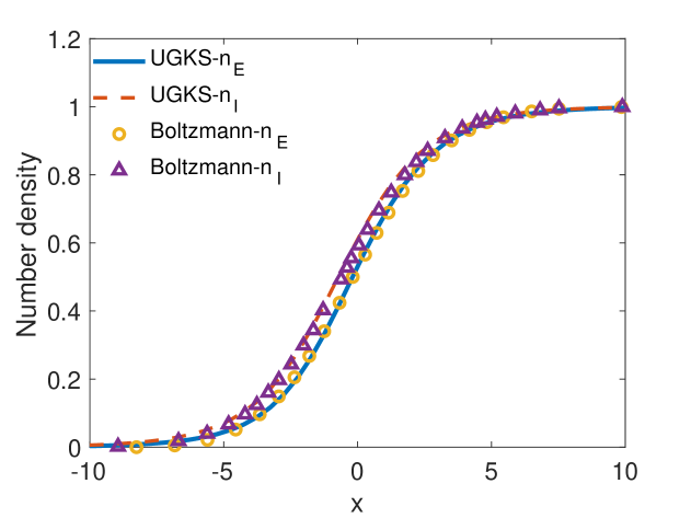
((a))

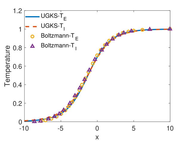
((b))

Figure 1: Shock structure at ${\rm Ma}_{\infty}=1.5$. Distributions of the (a) number densities and the (b) temperatures of electron and ion with the mass ratio $m_{\mathcal{E}}/m_{\mathcal{I}}=0.25$ and number density ratio $n_{\mathcal{E}}/n_{\mathcal{I}}=0.1$, solved by UGKS with the multispecies kinetic model compared with the result solved by Boltzmann equation [38].

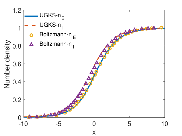
((a))

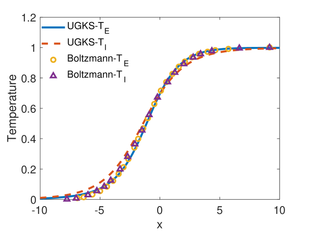
((b))

Figure 2: Shock structure at ${\rm Ma}_{\infty}=1.5$. Distributions of the (a) number densities and the (b) temperatures of electron and ion with the mass ratio $m_{\mathcal{E}}/m_{\mathcal{I}}=0.25$ and number density ratio $n_{\mathcal{E}}/n_{\mathcal{I}}=0.9$, solved by UGKS with the multispecies kinetic model compared with the result solved by Boltzmann equation [38].

4.2 Marshak wave

To further evaluate the capability of the current scheme in capturing the radiative equilibrium diffusion solution under conditions of optically thick limit, we impose a zero fluid velocity and maintain energy exchange between the material and radiation. The absorption/emission coefficient is $\sigma=100/T^{3}$. The initial condition of material temperature is $T_{\mathcal{E}}=10^{-4}$. And the initial condition for radiation field is $I(x)=0,x\in(0,1),I(0)=1,I(1)=0,$. The physical space is discretized with 200 uniform meshes and the solid angle space is with 30 points by midpoint rule. The range of solid angle space is $\Omega_{x}\in(-1,1)$. The result is shown in Fig. 3

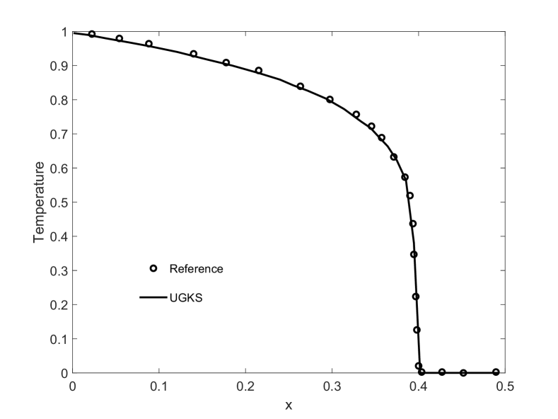
Figure 3: Marshak wave case whit $\sigma=100/T^{3}$, solved by UGKS with the kinetic model compared with the result solved by diffusion limit solution [35].

4.3 Radiative shock for $\rm{Ma}=1.5$ and $\rm{Ma}=3.0$

The newly developed multiscale method will be tested by two radiative shock cases, which have been studied in [39] and [40]. The radiation intensity is initialized according to the electron temperature. The physical space is discretized with 200 uniform meshes and the solid space is with 30 points by midpoint rule. The range of solid angle space is $\Omega_{x}\in(-1,1)$. Fig. 4 shows the density velocity and temperature of electron and ion and also radiation temperature for the Mach number $\rm{Ma}=1.5$ and mass ratio $m_{\mathcal{E}}/m_{\mathcal{I}}=1.0$. In the numerical solution, we observe a discontinuity in the fluid temperature due to the hydrodynamic shock, and the maximum temperature is bounded by the far-downstream temperature. This matches with the results in [40, 39]. Fig. 5 shows the density velocity and temperature of electron, ion, and also radiation temperature for the $\rm{Ma}=3.0$ and mass ratio $m_{\mathcal{E}}/m_{\mathcal{I}}=1.0$. For the strong shock, the material temperature reaches its maximum at the post-shock state, this point is called the Zel’dovich spike. In this case, both hydrodynamic shock and Zel’dovich spike appear which matches with the result [40, 39].

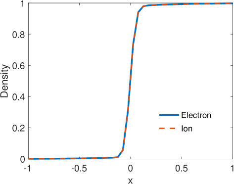
((a))

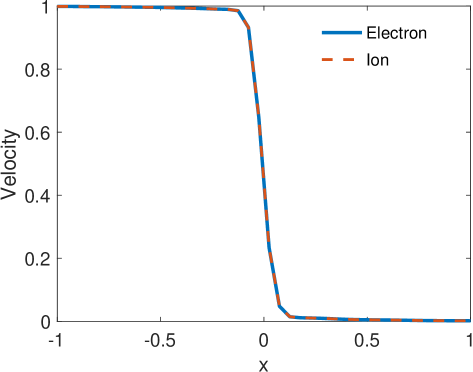
((b))

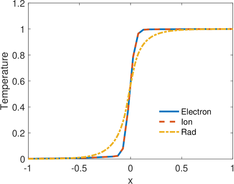
((c))

Figure 4: Distributions of the radiative shock (a) density, (b) velocity, and (c) temperature with Mach number $\rm{Ma}=1.5$ and mass ratio $m_{\mathcal{E}}/m_{\mathcal{I}}=1.0$.

((a))

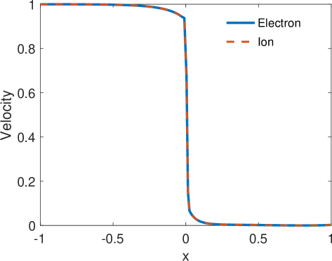
((b))

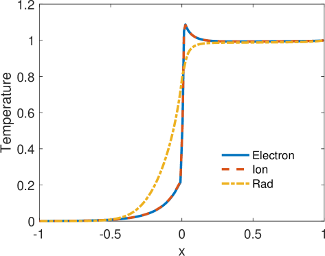
((c))

Figure 5: Distributions of the radiative shock (a) density, (b) velocity, and (c) temperature with Mach number $\rm{Ma}=3.0$ and mass ratio $m_{\mathcal{E}}/m_{\mathcal{I}}=1.0$.

4.4 Tophat for radiation plasma system

The two-dimensional Tophat problem is calculated to verify the capability to capture the extreme non-equilibrium physics in both optically thick/thin regimes with different mass and number density ratios of ion and electron. In the Tophat case, strong discontinuity is set in terms of both ${\rm Kn}$ number and $\sigma$ number. Shown in Fig. 6, the initial condition is set as an optically thick and continuum flow regime with $\sigma=10^{2},\rho=1.0,p=1.0,$ in $[x_{1},x_{2}]\times[y_{1},y_{2}]\in\{[3.0,4.0]\times[0,1.0],[0,2.5]\times[0.5,2.0],[4.5,7m_{.}0]\times[0.5,2.0],[2.5,4.5]\times[1.5,2.0]\}$, and an optical thin and free molecular flow regime with $\sigma=10^{-1},\rho=10^{-5},p=10^{-5}$ otherwise. And the mass and number density ratio of electron and ion is $rM=\frac{m_{\mathcal{I}}}{m_{\mathcal{E}}}=4.0,\frac{n_{\mathcal{I}}}{n_{\mathcal{E}}+n_{\mathcal{I}}}=0.2$.

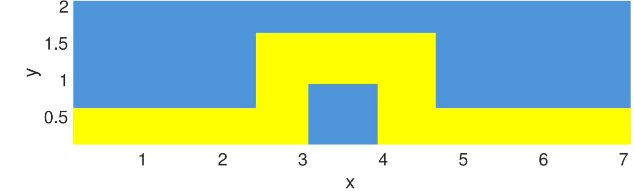
Figure 6: The demonstration of the initial settings of the two-dimensional Topha problem. Blue region represents the optical thick and continuum flow regime and yellow region represents the optical thin and free molecular flow regime.

The Knudsen number is defined by Eq. (33), where $L_{ref}=1$, and the reference mean free path is calculated by the number density and molecular diameter for mean free path calculation is $n=n_{\mathcal{I}}+n_{\mathcal{E}}$ and $d=d_{\mathcal{I}}=d_{\mathcal{E}}$. The physical space $x\times y=7\times 2$ is discretized by $70\times 20$ uniform meshes. The velocity space is discretized by $30\times 30$ points using the midpoint rule with the range $u_{\alpha}\in[-7,7]$ according to the most probable speed of each species $\alpha$.

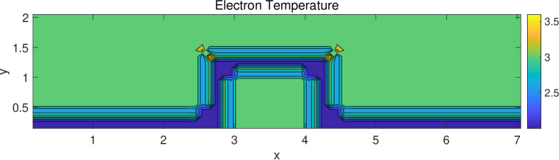
((a))

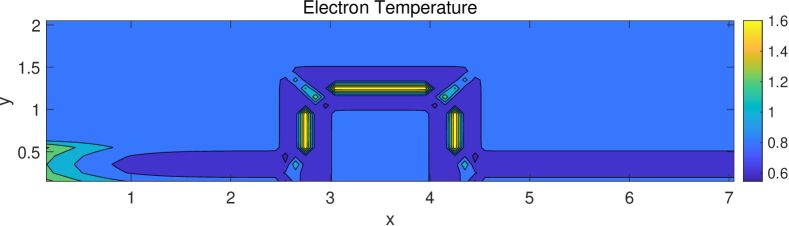
((b))

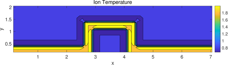
((c))

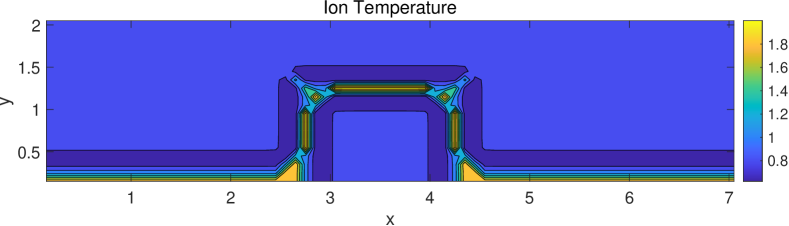
((d))

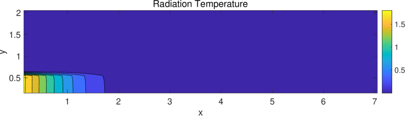
((e))

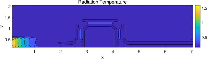
((f))

Figure 7: Two-dimensional Tophat problem with the mass ratio $m_{\mathcal{I}}/m_{\mathcal{E}}=4.0$ and number density ratio $n_{\mathcal{I}}/(n_{\mathcal{E}}+n_{\mathcal{I}})=0.2$. Distributions of electron temperature, ion temperature, and radiation temperature at $t=0.01$. The left figure a,c,e are results without exchange with radiation field while the right figure b,d,f are results of radiation plasma sytem

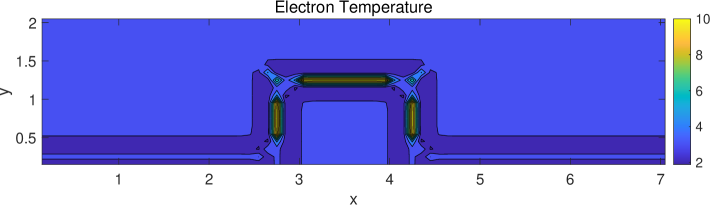
((a))

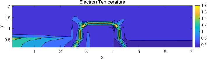
((b))

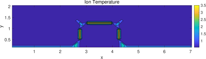
((c))

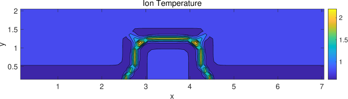
((d))

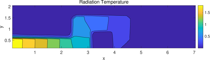
((e))

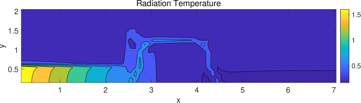
((f))

Figure 8: Two-dimensional Tophat problem with the mass ratio $m_{\mathcal{I}}/m_{\mathcal{E}}=4.0$ and number density ratio $n_{\mathcal{I}}/(n_{\mathcal{E}}+n_{\mathcal{I}})=0.2$. Distributions of electron temperature, ion temperature, and radiation temperature at $t=0.1$. The left figure a,c,e are results without exchange with radiation field while the right figure b,d,f are results of radiation plasma sytem

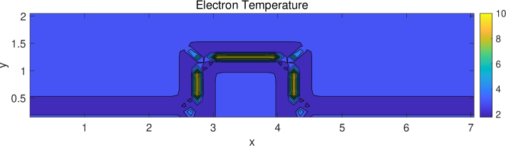
((a))

((b))

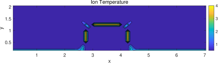
((c))

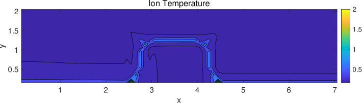
((d))

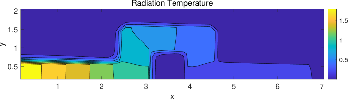
((e))

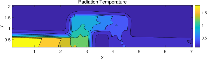
((f))

Figure 9: Two-dimensional Tophat problem with the mass ratio $m_{\mathcal{I}}/m_{\mathcal{E}}=4.0$ and number density ratio $n_{\mathcal{I}}/(n_{\mathcal{E}}+n_{\mathcal{I}})=0.2$. Distributions of electron temperature, ion temperature, and radiation temperature at $t=0.2$. The left figure a,c,e are results without exchange with radiation field while the right figure b,d,f are results of radiation plasma sytem

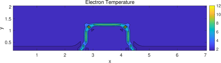
((a))

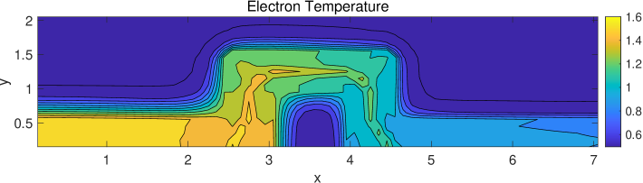
((b))

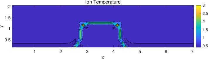
((c))

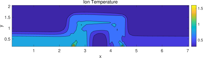
((d))

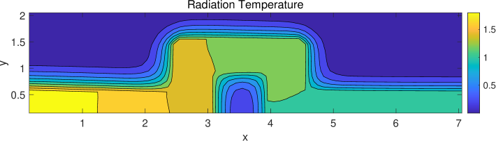
((e))

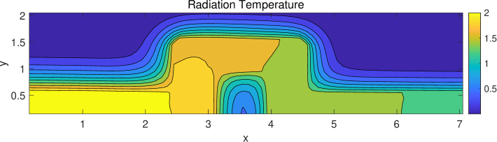
((f))

Figure 10: Two-dimensional Tophat problem with the mass ratio $m_{\mathcal{I}}/m_{\mathcal{E}}=4.0$ and number density ratio $n_{\mathcal{I}}/(n_{\mathcal{E}}+n_{\mathcal{I}})=0.2$. Distributions of electron temperature, ion temperature, and radiation temperature at $t=1.0$. The left figure a,c,e are results without exchange with radiation field while the right figure b,d,f are results of radiation plasma sytem

The results at times $t=0.01,0.1,0.2,1.0$ are selected to demonstrate the evolution of this problem. Initially, the macroscopic density, velocity, and pressure of ions and electrons are identical. However, due to variations in microscopic mass and number density, the temperatures of ions and electrons differ, as illustrated in Fig. 7. Moreover, it is observed that at the early stage of evolution, significant discontinuities in the fluid field rapidly evolve through interaction waves at the four corners for both ions and electrons. A comparison of Fig. 8 reveals that the radiation field’s evolution first impacts the electron temperature, subsequently affecting the ion temperature as well. The result is reasonable because the electronic component in the model equation exchanges energy with radiation, rather than the ionic component. When the radiation perturbation reaches the corners where electron and ion interactions are strong, the symmetrical structure of these corners is disrupted, as shown in Fig. 9. Additionally, the results indicate that when radiation temperature significantly influences both electron and ion temperatures, the interaction waves caused by strong discontinuities dissipate during the evolution. At this point, radiation temperature strongly influences the flow fields. This not only confirms the ability of our model to address non-equilibrium flows that involve multiscale transfer processes but also proves the necessity of developing a system with an interaction model. Fig. 10 illustrates that as time progresses, the radiation temperature gradually stabilizes while the symmetrical structure of electron and ion temperatures is progressively restored.

5 Conclusion

In this paper, we have developed a comprehensive framework for simulating multiscale physics in radiation-plasma systems. Our extended unified gas-kinetic scheme (UGKS) effectively models the temporal evolution of coupled radiation, electron, and ion interactions. The method addresses the challenge of varying fluid opacity across different regions by accurately capturing radiative transfer processes from free streaming to diffusive regimes. The approach incorporates a dual fluid model for electrons and ions while maintaining a nonequilibrium transport model for radiation, enabling precise computation of momentum and energy exchanges among these components. Our method demonstrates consistency with classical radiation hydrodynamic equations in the hydrodynamic limit. The multiscale transport capabilities of UGKS enable accurate resolution of radiative transfer across the entire spectrum, from optically thick to optically thin regimes. This comprehensive treatment not only reproduces the gray radiation limit but also provides enhanced resolution of multiscale phenomena, offering closer alignment with physical reality. The developed framework serves as a powerful computational tool for investigating radiation-plasma problems in astrophysics and inertial confinement fusion across diverse energy density regimes. Extensive numerical validation through various test cases demonstrates the scheme’s robustness and effectiveness in modeling complex radiation-plasma interactions. The method’s ability to resolve both equilibrium and nonequilibrium interactions in radiation-plasma systems represents a significant advancement in our capacity to understand and simulate multiscale dynamics in these complex physical systems. This work establishes a foundation for future investigations into radiation-plasma phenomena and offers new possibilities for studying previously challenging multiscale problems in related fields. The unified treatment provided by our approach promises to enhance both computational efficiency and physical accuracy in radiation-plasma simulations.

Author’s contributions

All authors contributed equally to this work.

Data Availability

The data that support the findings of this study are available from the corresponding author upon reasonable request.

References

- [1] R. P. Drake, Radiation Hydrodynamics, Springer Berlin Heidelberg, Berlin, Heidelberg, 2006, pp. 267–334.
- [2] D. Mihalas, B. Weibel-Mihalas, Foundations of radiation hydrodynamics, Courier Corporation, 1999.
- [3] S. Atzeni, J. Meyer-ter Vehn, The Physics of Inertial Fusion: BeamPlasma Interaction, Hydrodynamics, Hot Dense Matter, Oxford University Press, 2004.
- [4] C. Sijoy, S. Chaturvedi, Trhd: Three-temperature radiation-hydrodynamics code with an implicit non-equilibrium radiation transport using a cell-centered monotonic finite volume scheme on unstructured-grids, Computer Physics Communications 190 (2015) 98–119.
- [5] T. Di Matteo, E. Blackman, A. Fabian, Two-temperature coronae in active galactic nuclei, Monthly Notices of the Royal Astronomical Society 291 (1) (1997) L23–L27.
- [6] Y.-F. Jiang, J. M. Stone, S. W. Davis, Super-eddington accretion disks around supermassive black holes, The Astrophysical Journal 880 (2) (2019) 67.
- [7] M. Rampp, H.-T. Janka, Radiation hydrodynamics with neutrinos-variable eddington factor method for core-collapse supernova simulations, Astronomy & Astrophysics 396 (1) (2002) 361–392.
- [8] G. S. Fraley, E. J. Linnebur, R. J. Mason, R. L. Morse, Thermonuclear burn characteristics of compressed deuterium-tritium microspheres, Physics of Fluids 17 (2) (1974) 474–489.
- [9] E. L. Dewald, L. J. Suter, O. L. Landen, J. P. Holder, J. Schein, F. D. Lee, K. M. Campbell, F. A. Weber, D. G. Pellinen, M. B. Schneider, J. R. Celeste, J. W. McDonald, J. M. Foster, C. Niemann, A. J. Mackinnon, S. H. Glenzer, B. K. Young, C. A. Haynam, M. J. Shaw, R. E. Turner, D. Froula, R. L. Kauffman, B. R. Thomas, L. J. Atherton, R. E. Bonanno, S. N. Dixit, D. C. Eder, G. Holtmeier, D. H. Kalantar, A. E. Koniges, B. J. MacGowan, K. R. Manes, D. H. Munro, J. R. Murray, T. G. Parham, K. Piston, B. M. Van Wonterghem, R. J. Wallace, P. J. Wegner, P. K. Whitman, B. A. Hammel, E. I. Moses, Radiation-driven hydrodynamics of high- hohlraums on the national ignition facility, Phys. Rev. Lett. 95 (2005) 215004.
- [10] A. B. Wollaber, Four decades of implicit monte carlo, Journal of Computational and Theoretical Transport 45 (1-2) (2016) 1–70.
- [11] T. M. Evans, J. D. Densmore, Methods for coupling radiation, ion, and electron energies in grey implicit monte carlo, Journal of Computational Physics 225 (2) (2007) 1695–1720.
- [12] A. B. Wollaber, E. W. Larsen, J. D. Densmore, A discrete maximum principle for the implicit monte carlo equations, Nuclear Science and Engineering 173 (3) (2013) 259–275.
- [13] C. Enaux, S. Guisset, C. Lasuen, G. Samba, Numerical methods for coupling multigroup radiation with ion and electron temperatures, Communications in Applied Mathematics and Computational Science 17 (1) (2022) 43–78.
- [14] G. Peng, Z. Gao, X. Feng, An extremum-preserving finite volume scheme for three-temperature radiation diffusion equations, Mathematical Methods in the Applied Sciences 45 (8) (2022) 4643–4660.
- [15] J. Cheng, N. Lei, C.-W. Shu, High order conservative lagrangian scheme for three-temperature radiation hydrodynamics, Journal of Computational Physics 496 (2024) 112595.
- [16] R. Lowrie, J. Morel, J. Hittinger, The coupling of radiation and hydrodynamics, The astrophysical journal 521 (1) (1999) 432.
- [17] B. Van der Holst, G. Tóth, I. V. Sokolov, K. G. Powell, J. P. Holloway, E. Myra, Q. Stout, M. Adams, J. Morel, S. Karni, et al., Crash: A block-adaptive-mesh code for radiative shock hydrodynamics—implementation and verification, The Astrophysical Journal Supplement Series 194 (2) (2011) 23.
- [18] W. Sun, S. Jiang, K. Xu, G. Cao, Multiscale simulation for the system of radiation hydrodynamics, Journal of Scientific Computing 85 (2020) 1–24.
- [19] S. M. Kolb, M. Stute, W. Kley, A. Mignone, Radiation hydrodynamics integrated in the pluto code, Astronomy & Astrophysics 559 (2013) A80.
- [20] N. Moens, J. Sundqvist, I. El Mellah, L. Poniatowski, J. Teunissen, R. Keppens, Radiation-hydrodynamics with mpi-amrvac-flux-limited diffusion, Astronomy & Astrophysics 657 (2022) A81.
- [21] B. Commerçon, R. Teyssier, E. Audit, P. Hennebelle, G. Chabrier, Radiation hydrodynamics with adaptive mesh refinement and application to prestellar core collapse-i. methods, Astronomy & Astrophysics 529 (2011) A35.
- [22] Y.-F. Jiang, J. M. Stone, S. W. Davis, A global three-dimensional radiation magneto-hydrodynamic simulation of super-eddington accretion disks, The Astrophysical Journal 796 (2) (2014) 106.
- [23] Y.-F. Jiang, J. M. Stone, S. W. Davis, Radiation magnetohydrodynamic simulations of the formation of hot accretion disk coronae, The Astrophysical Journal 784 (2) (2014) 169.
- [24] Y.-F. Jiang, O. Blaes, J. M. Stone, S. W. Davis, Global radiation magnetohydrodynamic simulations of sub-eddington accretion disks around supermassive black holes, The Astrophysical Journal 885 (2) (2019) 144.
- [25] K. Xu, J.-C. Huang, A unified gas-kinetic scheme for continuum and rarefied flows, Journal of Computational Physics 229 (20) (2010) 7747–7764.
- [26] K. Xu, Direct modeling for computational fluid dynamics: construction and application of unified gas-kinetic schemes, Vol. 4, World Scientific, 2014.
- [27] G. A. Bird, Molecular gas dynamics and the direct simulation of gas flows, Oxford university press, 1994.
- [28] J. E. Broadwell, Study of rarefied shear flow by the discrete velocity method, Journal of Fluid Mechanics 19 (3) (1964) 401–414.
- [29] S. Liu, P. Yu, K. Xu, C. Zhong, Unified gas-kinetic scheme for diatomic molecular simulations in all flow regimes, Journal of Computational Physics 259 (2014) 96–113.
- [30] Z. Wang, H. Yan, Q. Li, K. Xu, Unified gas-kinetic scheme for diatomic molecular flow with translational, rotational, and vibrational modes, Journal of Computational Physics 350 (2017) 237–259.
- [31] T. Xiao, K. Xu, Q. Cai, A unified gas-kinetic scheme for multiscale and multicomponent flow transport, Applied Mathematics and Mechanics 40 (3) (2019) 355–372.
- [32] R. Wang, K. Xu, Unified gas-kinetic scheme for multi-species non-equilibrium flow, in: AIP Conference Proceedings, Vol. 1628, American Institute of Physics, 2014, pp. 970–975.
- [33] C. Liu, K. Xu, A unified gas kinetic scheme for continuum and rarefied flows v: Multiscale and multi-component plasma transport, Communications in Computational Physics 22 (5) (2017) 1175–1223.
- [34] L. Mieussens, On the asymptotic preserving property of the unified gas kinetic scheme for the diffusion limit of linear kinetic models, Journal of Computational Physics 253 (2013) 138–156.
- [35] W. Sun, S. Jiang, K. Xu, An asymptotic preserving unified gas kinetic scheme for gray radiative transfer equations, Journal of Computational Physics 285 (2015) 265–279.
- [36] W. Sun, S. Jiang, K. Xu, S. Li, An asymptotic preserving unified gas kinetic scheme for frequency-dependent radiative transfer equations, Journal of Computational Physics 302 (2015) 222–238.
- [37] P. Andries, K. Aoki, B. Perthame, A consistent bgk-type model for gas mixtures, Journal of Statistical Physics 106 (2002) 993–1018.
- [38] S. Kosuge, K. Aoki, S. Takata, Shock-wave structure for a binary gas mixture: finite-difference analysis of the boltzmann equation for hard-sphere molecules, European Journal of Mechanics-B/Fluids 20 (1) (2001) 87–126.
- [39] S. Bolding, J. Hansel, J. D. Edwards, J. E. Morel, R. B. Lowrie, Second-order discretization in space and time for radiation-hydrodynamics, Journal of Computational Physics 338 (2017) 511–526.
- [40] R. B. Lowrie, J. D. Edwards, Radiative shock solutions with grey nonequilibrium diffusion, Shock waves 18 (2008) 129–143.