Iterative Prompt Relocation for Distribution-Adaptive Visual Prompt Tuning

Abstract

Visual prompt tuning (VPT) provides an efficient and effective solution for adapting pre-trained models to various downstream tasks by incorporating learnable prompts. However, most prior art indiscriminately applies a fixed prompt distribution across different tasks, neglecting the importance of each block differing depending on the task. In this paper, we investigate adaptive distribution optimization (ADO) by addressing two key questions: (1) How to appropriately and formally define ADO, and (2) How to design an adaptive distribution strategy guided by this definition? Through in-depth analysis, we provide an affirmative answer that properly adjusting the distribution significantly improves VPT performance, and further uncover a key insight that a nested relationship exists between ADO and VPT. Based on these findings, we propose a new VPT framework, termed PRO-VPT (iterative Prompt RelOcation-based VPT), which adaptively adjusts the distribution building upon a nested optimization formulation. Specifically, we develop a prompt relocation strategy for ADO derived from this formulation, comprising two optimization steps: identifying and pruning idle prompts, followed by determining the optimal blocks for their relocation. By iteratively performing prompt relocation and VPT, our proposal adaptively learns the optimal prompt distribution, thereby unlocking the full potential of VPT. Extensive experiments demonstrate that our proposal significantly outperforms state-of-the-art VPT methods, e.g., PRO-VPT surpasses VPT by 1.6% average accuracy, leading prompt-based methods to state-of-the-art performance on the VTAB-1k benchmark. The code is available at https://github.com/ckshang/PRO-VPT.

1 Introduction

Fine-tuning pre-trained vision models (PVMs) [24] has proven remarkably effective in adapting to a variety of downstream tasks [58, 14]. However, the computational and storage costs associated with full fine-tuning are prohibitively high, particularly as model sizes continue to grow [37, 52, 1]. To overcome these challenges, parameter-efficient fine-tuning (PEFT) methods [55, 56, 18, 2], such as visual prompt tuning (VPT) [20], have emerged as more promising alternatives, garnering significant attention.

Figure 1: PRO-VPT (ours) vs. prior art in VPT. Existing VPT approaches typically insert trainable prompts into the PVM with a pre-specific static distribution, whether shallow or deep, and optimize these prompts to drive the PVM to conduct downstream tasks. Compared to the prior art, our proposal (PRO-VPT) adaptively adjusts prompt distribution by treating it as an optimization objective and coupling the distribution optimization with prompt tuning.

Instead of updating all model parameters directly, VPT inserts learnable prompt tokens into the input space of Transformer blocks, with either a shallow distribution (inserted only in the first block) or a deep distribution (uniformly inserted across all blocks), while keeping the PVM frozen. This approach significantly reduces the number of parameters that need to be fine-tuned, thereby lowering the computational and memory overhead [14]. Follow-up research further enhances this pipeline by improving aspects such as prompting architecture [13, 46], prompt initialization [53], and the propagation structures of prompts [62, 57, 5].

Despite these advancements, most of the prior art still relies on a preset fixed prompt distribution, either shallow or deep, across various downstream tasks, as illustrated in Fig. 1. However, recent findings reveal that the importance of each block varies significantly across different tasks [45, 41, 12, 26, 54], underscoring the need to dynamically tailor the fine-tuning intensity for each block to improve task performance [27, 48, 11, 42, 23]. This implies that indiscriminately using a fixed prompt distribution is inadequate, motivating us to adaptively adjust the distribution to better accommodate each task.

In this paper, we naturally consider prompt distribution as one of the optimization objectives, which we refer to as adaptive distribution optimization (ADO). As the focus pivots towards the ADO problem, new questions arise. First, given the unexplored nature of prompt distribution optimization, the definition of ADO remains unclear. For instance, defining it as a one-shot process or an iterative one leads to a critical consideration, namely whether the effectiveness of distribution adjustments is influenced by ongoing prompt updates. This leads us to our first key question: How can we appropriately and formally define ADO? Second, once the definition of ADO is established, a more essential question emerges: How can we achieve adaptive distribution derived from this definition?

To address these questions, we first empirically analyze the ADO problem. Our findings confirm the significance of ADO and further highlight two key insights: the effectiveness of distribution adjustments is indeed impacted by prompt updates, and a nested relationship exists between ADO and VPT. To this end, we propose a novel iterative framework, termed PRO-VPT (iterative Prompt RelOcation-based VPT), with a nested optimization definition for ADO and VPT. Specifically, building on this definition, we develop a prompt relocation (PR) strategy for adaptively refining the distribution. It comprises two key optimization steps: pruning and allocating. The pruning step first identifies and releases idle prompts, while the subsequent allocation step determines optimal blocks for redistributing these prompts. By iteratively executing PR and VPT, the proposed PRO-VPT adaptively learns the optimal prompt distribution for each task, unlocking the full potential of VPT and leading to improved robustness. Our contributions can be summarized as follows:

• We explore the ADO problem within VPT and reveal the nested relationship between ADO and VPT.

• Building upon our insights into prompt distribution, we propose the first ADO-VPT co-design framework, termed PRO-VPT, with a nested optimization definition.

• Derived from the definition, we present a PR strategy for ADO, which introduces an idleness score to prune underutilized prompts and allocate them to more effective blocks using reinforcement learning (RL).

• Extensive experiments show that PRO-VPT reaches the state-of-the-art average accuracy of 78.0% on VTAB-1k, with a 1.6% advantage over the VPT baseline.

2 Related Work

Visual Prompt Tuning. VPT [20], one of the leading techniques in PEFT, draws inspiration from language-domain prompting works [37, 34, 29, 35] to fine-tune a small portion of prompts while keeping the pre-trained vision Transformer (ViT) frozen. Subsequent research has improved VPT in three main aspects: (1) Extending prompts to other Transformer components (e.g., key and value matrices or the patch embedding layer) to better suit the Transformer architecture [13, 46]; (2) Initializing prompts with prototypes of image tokens to accelerate convergence [53]; (3) Refining the propagation structures of prompts to strengthen cross-layer interactions [62, 57, 5]. However, most existing methods depend on a fixed prompt distribution across different tasks, resulting in less effective prompting solutions. In contrast, our approach adaptively adjusts the prompt distribution for each task, enabling prompt-based methods to achieve advanced performance.

Layer-wise fine-tuning. Resent research [49, 28, 12] has highlighted the importance of recognizing the varying contributions of pre-trained blocks for enhancing fine-tuning performance and robustness. For instance, [27] demonstrates that identifying pre-trained blocks that are already near-optimal for the downstream task and selectively fine-tuning the remaining blocks can significantly improve robustness to distribution shifts. Similarly, [45] shows that assigning different learning rates for each block is advantageous for few-shot learning. Furthermore, TPGM [48] introduces a bi-level optimization to optimize a projection constraint for each block, aiming to learn how much to fine-tune each block. Inspired by these findings, we hypothesize that the prompting intensity for each block, i.e., the overall distribution of prompts, may also play a crucial role in task adaptation, leading us to focus on adaptively adjusting the prompt distribution within VPT.

3 Methodology

3.1 Motivation

Many previous studies have emphasized the significance of treating each Transformer block differently during downstream task fine-tuning [45, 27, 12, 23]. For instance, a notable study in [27] reveals that certain blocks pre-trained on the upstream task may already be near-optimal for specific downstream tasks, hence over-tuning could impair generalization. As a result, recent advances have focused on developing adaptive fine-tuning strategies to calibrate the fine-tuning intensity for each block, which have shown promising potential in improving both performance and robustness [41, 49]. This suggests that utilizing a fixed prompt distribution (essentially the number of prompts/prompting intensity per block) for all tasks, without any differentiation, might not fully exploit the potential of VPT. Motivated by this insight, our work focuses on optimizing the prompt distribution to better accommodate downstream tasks and enhance overall robustness (cf. § 4.5).

3.2 Analysis and Formulation of ADO

We first examine the underlying nature of ADO and its precise formulation. Intuitively, ADO can be defined in two distinct ways: one-shot (independently adjusting the distribution) or iterative (integrating with prompt tuning through iteratively adjusting the distribution). These definitions are distinct in whether the distribution is adjusted concurrently with prompt tuning. Specifically, an iterative process is more suitable if distribution adjustments are influenced by ongoing prompt updates, as independent optimization might lead to suboptimal results without accounting for these changes. Conversely, one-shot adjustments may suffice if the adjustments remain unaffected by prompt updates.

Figure 2: Performance gaps from distribution adjustments using prompts from epochs 25, 50, and 75. Adjusting prompt distribution appropriately leads to enhanced performance; however, effective adjustments vary significantly across different epochs.

To investigate which definition better matches the underlying nature, we experiment to observe how distribution adjustments perform when applied to prompts from different epochs. We use two intuitive adjustment strategies: incrementally adding to a small initial prompt set and repositioning existing prompts. As shown in Fig. 2, adding or repositioning prompts to specific blocks can effectively improve performance; however, the effective adjustments differ significantly when prompts are updated. Comprehensive analysis with detailed results is provided in Appendix B. In conclusion, we summarize our key discoveries as follows:

Discovery 1. Properly adjusting the prompt distribution significantly enhances performance, confirming the necessity to reconsider its optimization.

Discovery 2. The effectiveness of distribution adjustments is sensitive not only to different blocks but also to the updated prompts themselves, highlighting the need for an iterative process that continuously adjusts the distribution over time.

Discovery 3. Distribution adjustments can only be properly evaluated after prompt tuning, indicating that the prompt tuning process should be nested within the distribution optimization process (see Appendix B).

Building on these insights, we propose integrating ADO with VPT into an iterative optimization framework. Formally, we present the definition of this ADO-VPT co-design framework through the lens of nested optimization. Let $\mathbf{P}\!=\!\{\mathbf{p}_{k}\}^{N}_{k=1}$ denote a set of $N$ prompts and $\mathcal{D}\!=\!\{d_{k}\}^{N}_{k=1}$ represent their distributed blocks, the objectives of ADO and VPT can then be expressed as:

$$\mathcal{D}^{\ast} =\mathop{\arg\min}\limits_{\mathcal{D}}\leavevmode\nobreak\ \mathbb{E}_{(\mathbf{x},y)\in\mathcal{T}_{tr}}\big{[}\mathcal{L}(f_{\mathbf{P}^{\ast},\mathcal{D}}(\mathbf{x}),y)\big{]},$$ (1)

$$\mathbf{P}^{\ast} =\mathop{\arg\min}\limits_{\mathbf{P}}\leavevmode\nobreak\ \mathbb{E}_{(\mathbf{x},y)\in\mathcal{T}_{tr}}\big{[}\mathcal{L}(f_{\mathbf{P},\mathcal{D}^{\ast}}(\mathbf{x}),y)\big{]},$$ (2)

where $d_{k}\!\in\!\{0\}\!\bigcup[L]$ ($d_{k}\!=\!0$ for undistributed) and $L$ denotes the number of Transformer blocks $\{B_{i}\}^{L}_{i=1}$. $\mathcal{T}_{tr}$ is the training set with input-label pairs $(\mathbf{x},y)$, $\mathcal{L}$ is the task loss function, and $f_{\mathbf{P},\mathcal{D}}$ is the prompted model. This formulation clearly illustrates the intertwined relationship between visual prompts $\mathbf{P}$ and their distribution $\mathcal{D}$, with its workflow presented in Fig. iii. A more detailed explanation for this nested optimization formulation is provided in Appendix B.

Figure 3: Overview of our proposed PRO-VPT. Left: The streamlined workflow of PRO-VPT. Right: Illustration of the PR process.

To solve this nested optimization, we employ the alternating optimization approach [1], establishing an iterative process that alternates between ADO and VPT. Specific to ADO, we empirically observe that adding-based adjustments may lead to undertraining of newly introduced prompts and conflicts with existing ones, as illustrated in Appendix C. Therefore, we particularly focus on developing a prompt relocation (PR) strategy derived from the formulation to effectively tackle the ADO problem.

3.3 Iterative Prompt Relocation-based VPT

Since the objective of PR defined in Eq. (1) poses a discrete optimization problem that cannot be directly solved by backpropagation, we first introduce the PR strategy derived from the definition, followed by a detailed overview of the PRO-VPT framework. Building on our discoveries regarding ADO, the discrete PR objective is further complicated by the non-stationary nature of effective relocation (Discovery 2) and the necessity to predict the effectiveness of various relocation operations (Discovery 3). Nevertheless, these three properties make a RL framework [30, 22] a natural and well-suited approach for optimizing the PR objective, where all possible relocation operations are treated as actions.

However, a naive RL implementation considering all $L^{2}$ possible relocation arrangements (e.g., 144 actions for ViT-B) would require numerous iterations to achieve convergence (cf. § 4.3). To address this, we propose decomposing the PR process into two sequential steps: pruning and allocating. The pruning step first identifies and releases idle prompts for relocation, while the allocating step then employs RL to determine optimal blocks for these freed prompts. By focusing merely on possible allocatable blocks for the pruned prompts, this approach effectively reduces the action space from $L^{2}$ to $L$. Formalizing this, the optimization objectives for pruning and allocation, derived from Eq. (1), are:

$$k^{\ast}=\ \mathop{\arg\max}\limits_{k}\leavevmode\nobreak\ \mathbb{E}_{(\mathbf{x},y)\in\mathcal{T}_{tr}}\big{[}\Delta\mathcal{L}(f_{\mathbf{P},\mathcal{D}},f_{\mathbf{P},\mathcal{D}\mid d_{k}=0})\big{]},$$ (3)

$$a^{\ast}=\ \mathop{\arg\max}\limits_{a}\leavevmode\nobreak\ \mathbb{E}_{(\mathbf{x},y)\in\mathcal{T}_{tr}}\big{[}\Delta\mathcal{L}(f_{\mathbf{P},\mathcal{D}^{-}},f_{\mathbf{P}^{\prime},\mathcal{D}\mid d_{k^{\!\ast\!}}=a})\big{]},$$ (4)

where $\Delta\mathcal{L}(f_{1},f_{2})\!=\!\mathcal{L}(f_{1}(\mathbf{x}),y)\!-\!\mathcal{L}(f_{2}(\mathbf{x}),y)$ denotes the loss difference, $\mathcal{D}^{-}\!=\!\{d_{k}\!\in\!\mathcal{D}\!\mid\!d_{k^{\!\ast\!}}\!=\!0\}$ and $\mathcal{D}^{+}\!=\!\{d_{k}\!\in\!\mathcal{D}\!\mid\!d_{k^{\!\ast\!}}\!=\!a^{\ast}\}$ represent the prompt distributions after pruning and allocation, with $a\!\in\![L]$ as the allocation block index. In accordance with Discovery 3, Eq. (4) evaluates the allocation step using the tuned prompts $\mathbf{P}^{\prime}$. Remarkably, both pruning and allocation steps operate on a single prompt per iteration, with further explanation provided in Appendix D.

Next, we approach these two stages around the optimization objectives as follows.

Idleness-Score-based Pruning. To quantify whether a prompt is idle and suitable for relocation, we introduce an idleness score $\mathcal{I}_{k}$ based on Eq. (3):

$$\mathcal{I}_{k}=\Delta\mathcal{L}(f_{\mathbf{P},\mathcal{D}},f_{\mathbf{P},\mathcal{D}\mid d_{k}=0}).$$ (5)

Clearly, if the idleness score $\mathcal{I}_{k}\!=\!\Delta\mathcal{L}\!>\!0$, the prompt $\mathbf{p}_{k}$ is more advantageous to prune than to retain, indicating that it is negative for the current model $f_{\mathbf{P},\mathcal{D}}$ and thereby can be pruned for potential relocation. Conversely, if $\mathcal{I}_{k}\!\leq\!0\leavevmode\nobreak\ \forall k$, no prompt is sufficiently idle to warrant removal.

Furthermore, since computing $\mathcal{I}_{k}$ for each individual prompt $\mathbf{p}_{k}$ is significantly inefficient, we approximate $\mathcal{I}_{k}$ using its first-order Taylor expansion (details are available in Appendix E):

$$\widehat{\mathcal{I}}_{k}\approx\mathbf{g}_{k}^{T}\mathbf{p}_{k},$$ (6)

where $\mathbf{g}_{k}\!=\!\frac{\nabla\mathcal{L}}{\nabla\mathbf{p}_{k}}$ represents the elements of the gradient $\mathbf{g}$.

Therefore, by calculating the estimated scores as in Eq. (6), we can effectively identify and release the idle prompt $\mathbf{p}_{k^{\!\ast\!}}$ if $\widehat{\mathcal{I}}_{k^{\!\ast\!}}\!=\!\max\widehat{\mathcal{I}}_{k}\!>\!0$, thereby forming $\mathcal{D}^{-}$.

RL-based Allocation. After pruning an idle prompt, the following key step is to leverage RL to determine its optimal allocation to the block where it can be more effective. Building on the allocation objective in Eq. (4), the optimization objective for the RL problem, i.e., the allocation reward, can be formulated as follows:

$$r=\Delta\mathcal{L}(f_{\mathbf{P},\mathcal{D}^{-}},f_{\mathbf{P}^{\prime},\mathcal{D}\mid d_{k^{\!\ast}\!=\!a}}).$$ (7)

We detail this RL problem under a Markov decision process framework, where the main components are:

1) State. We leverage all available information to represent the observations of each block’s prompts. Specifically, the state is defined as a concatenation of three elements: block-wise idleness scores, prompt distribution, and one-hot encoding of the pruned prompt’s location. Formally, the state is defined as $s\!=\!\{\sum_{d_{k}\!=\!i}\widehat{\mathcal{I}}_{k}\}_{i\!=\!1}^{L}\!\bigcup\!\mathcal{D}^{-}\!\bigcup\!\text{{OneHot}}(k^{\ast})$. After PR and VPT, the state transitions to $s^{\prime}$.

2) Action. The action determines which block the pruned prompt will be allocated to, represented as $a\in[L]$.

3) Reward. Although the allocation reward is defined in Eq. (7), calculating the intermediate loss of $f_{\mathbf{P},\mathcal{D}^{-}}$ is computationally inefficient. To address this, we reformulate the reward by incorporating the idleness score as:

$$\hat{r}\approx\Delta\mathcal{L}(f_{\mathbf{P},\mathcal{D}},f_{\mathbf{P}^{\prime},\mathcal{D}\mid d_{k^{\!\ast}\!=\!a}})-\widehat{\mathcal{I}}_{k^{\!\ast}},$$ (8)

where the idleness score $\widehat{\mathcal{I}}_{k^{\!\ast}}\!\approx\!\Delta\mathcal{L}(f_{\mathbf{P},\mathcal{D}},f_{\mathbf{P},\mathcal{D}^{-}})$ provides an approximation of the intermediate loss of $f_{\mathbf{P},\mathcal{D}^{-}}$.

By leveraging RL, we can efficiently determine the optimal allocation block for the pruned prompt, even within the non-stationary environment. We achieve this using proximal policy optimization (PPO) [44], a state-of-the-art RL algorithm. In particular, PPO learns a policy that identifies the optimal block to maximize the reward in Eq. (8).

Input: pre-trained model $f$, number of epochs $T$, number of prompts $N$, learning rate $\eta$.

1 Initialize $N$ prompts $\mathbf{P}$ and distribute them to the model according to a uniform distribution $\mathcal{D}$.

2 for $t=0,\ldots,T-1$ do

3    Compute idleness scores $\{\widehat{\mathcal{I}}_{k}\}^{N}_{k=1}$ by Eq. (6).

4    if $\max\widehat{\mathcal{I}}_{k}\!>\!0$ then

5       Prune the negative prompt $\mathbf{p}_{k^{\!\ast\!}}$ with the maximum idleness score $\widehat{\mathcal{I}}_{k^{\!\ast\!}}$ to form $\mathcal{D}^{-}$.

6       Compute the current state $s$.

7       Compute the action $a\leftarrow\text{PPO}(s)$.

8       Allocate the idle prompt $\mathbf{p}_{k^{\!\ast\!}}$ to the $a^{\text{th}}$ block to form $\mathcal{D}^{+}$.

9      

10    Update the prompts as $\mathbf{P}^{\prime}\leftarrow\mathbf{P}-\eta\cdot\mathbf{g}$.

11    if $\max\widehat{\mathcal{I}}_{k}\!>\!0$ then

12       Compute the reward $\hat{r}$ by Eq. (8).

13       Update the policy networks within PPO based on $\hat{r}$.

14   

Algorithm 1 The proposed PRO-VPT algorithm

Justification. Although we decompose the PR process into two-step sequential steps, the overall optimization objective, whether it is based on the expected objectives in Eqs. (3) and (4) or the estimated objectives in Eqs. (6) and (8), can be expressed as $\max_{a}\mathbb{E}_{(\mathbf{x},y)\in\mathcal{T}_{tr}}[\Delta\mathcal{L}(f_{\mathbf{P},\mathcal{D}},f_{\mathbf{P}^{\prime},\mathcal{D}\mid d_{k^{\!\ast}\!=\!a}})]$. This formulation remains equivalent to the original PR objective (i.e., the ADO objective) defined in Eq. (1). Consequently, leveraging the nested optimization formulation, the proposed PR strategy can effectively address the ADO problem and adaptively construct the optimal distribution for the entire prompt set.

Overall PRO-VPT Framework. Fig. 3 illustrates the streamlined process of PRO-VPT, and Algorithm 1 presents the detailed pseudocode.

3.4 Discussion

We note that some prior works have indirectly achieved adaptive distribution [13, 25, 60]. Specifically, pruning-based techniques [13, 25] introduce mask variables to iteratively prune redundant prompts from the original distribution, and NOAH [60] use an evolutionary algorithm to search for an optimal sub-structure within the original distribution in one-shot manner. Overall, these approaches aim to enhance performance through the lottery ticket hypothesis [8, 39], focusing on searching for a sub-distribution within a given hyper-distribution. PRO-VPT is distinct and advantageous compared to these methods as follows:

Distinct Goals. These methods primarily concentrate on circumventing negative prompts and retaining essential ones to enhance performance. In contrast, our approach actively learns an optimal distribution of all prompts, relocating them to maximize the effectiveness of each prompt. This fundamental distinction sets our approach apart from the methods discussed above.

Efficient. While effective, we argue that these approaches typically incur considerable unnecessary training costs, as numerous trained prompts are pruned and left unused (cf. § 4.3). This fundamentally contradicts the goal of parameter efficiency. Conversely, our work directly adjusts the distribution of the entire prompt set through prompt relocation, thereby minimizing extra costs and improving efficiency.

Effective. These methods straightforwardly apply one-shot or iterative processes without considering the underlying distribution dynamics. For example, NOAH adopts a one-shot approach post-training, leading to suboptimal results (cf. § 4.2). Conversely, our work conducts empirical analyzes and proposes a nested-optimization-based method, enabling prompt-based methods to reach state-of-the-art performance.

4 Experiments

Table 1: Detailed results on the VTAB-1k datasets. Performance results are reported as the highest of ImageNet normalization ($\circ$) or Inception normalization ($\bullet$), presented in % after a complete training schedule with ViT-B/16 supervised pre-trained on ImageNet-21k. The best results of prompt-based methods and other PEFT approaches are highlighted in bold. ↯: Early-stopping based on the test set. $\dagger$: Lack of complete code or hyperparameter configurations for the method, hence results are reported as presented in the original paper. ¹Average across the average accuracies of the VTAB-1k groups, following previous work.

		Natural								Specialized					Structured
	Param (M)	Cifar100	Caltech101	DTD	Flower102	Pets	SVHN	Sun397	Group Avg.	Camelyon	EuroSAT	Resisc45	Retinopathy	Group Avg.	Clevr-Count	Clevr-Dist.	DMLab	KITTI-Dist.	dSpr-Loc.	dSpr-Ori.	sNORB-Azi.	sNORB-Ele.	Group Avg.	Global Avg.1
Full $\bullet$	85.8	73.2	92.6	70.4	97.9	86.2	90.6	39.6	78.6	87.1	96.6	87.5	74.0	86.3	66.6	61.0	49.8	79.7	82.6	51.9	33.5	37.0	57.8	74.2
Linear $\bullet$	0.04	78.1	88.1	69.0	99.1	90.0	36.0	56.9	73.9	79.8	90.7	73.7	73.7	79.5	32.4	30.5	35.9	61.9	11.2	26.2	14.3	24.5	29.6	61.0
LoRA $\bullet$ [18]	0.29	83.0	91.7	71.6	99.2	90.9	83.8	56.7	82.4	86.2	95.7	83.5	71.9	84.3	77.7	62.3	49.0	80.2	82.2	51.7	31.0	47.0	60.1	75.6
$\text{FacT-TK}_{8}$ $\bullet$ [21]	0.05	74.9	92.7	73.7	99.1	91.3	85.5	57.7	82.1	86.8	94.9	84.1	70.9	84.2	81.9	64.1	49.2	77.2	83.8	53.1	28.2	44.7	60.3	75.5
FacT-TK≤32 $\bullet$ [21]	0.10	74.6	93.7	73.6	99.3	90.6	88.7	57.5	82.6	87.6	95.4	85.5	70.4	84.7	84.3	62.6	51.9	79.2	85.5	52.0	36.4	46.6	62.3	76.5
Consolidator $\dagger$ [15]	0.30	74.2	90.9	73.9	99.4	91.6	91.5	55.5	82.4	86.9	95.7	86.6	75.9	86.3	81.2	68.2	51.6	83.5	79.8	52.3	31.9	38.5	60.9	76.5
SSF ↯$\circ$ [31]	0.24	69.0	92.6	75.1	99.4	91.8	90.2	52.9	81.6	87.4	95.9	87.4	75.5	86.6	75.9	62.3	53.3	80.6	77.3	54.9	29.5	37.9	59.0	75.7
SPT-Adapter ↯$\circ$ [16]	0.23	72.9	93.2	72.5	99.3	91.4	84.6	55.2	81.3	85.3	96.0	84.3	75.5	85.3	82.2	68.0	49.3	80.0	82.4	51.9	31.7	41.2	60.8	75.8
SPT-Adapter ↯$\circ$ [16]	0.43	72.9	93.2	72.5	99.3	91.4	88.8	55.8	82.0	86.2	96.1	85.5	75.5	85.8	83.0	68.0	51.9	81.2	82.4	51.9	31.7	41.2	61.4	76.4
Adapter+r=16 $\bullet$ [47]	0.35	83.7	94.2	71.5	99.3	90.6	88.2	55.8	83.3	87.5	97.0	87.4	72.9	86.2	82.9	60.9	53.7	80.8	88.4	55.2	37.3	46.9	63.3	77.6
Prompt-based Methods:
VPT-Deep $\bullet$ [20]	0.60	83.0	93.0	71.2	99.0	91.3	84.1	56.0	82.5	84.9	96.6	82.5	74.5	84.6	77.5	58.7	49.7	79.6	86.2	56.1	37.9	50.7	62.1	76.4
NOAH ↯$\mathbin{\vphantom{\circ}\text{\ooalign{\clipbox{0 0 0 {}}{$\bullet$}\cr$\circ$\cr}}}$ [60]	0.43	69.6	92.7	70.2	99.1	90.4	86.1	53.7	80.2	84.4	95.4	83.9	75.8	84.9	82.8	68.9	49.9	81.7	81.8	48.3	32.8	44.2	61.3	75.5
SPT-Deep $\dagger$ [53]	0.22	79.3	92.6	73.2	99.5	91.0	89.1	51.2	82.3	85.4	96.8	84.9	74.8	85.5	70.3	64.8	54.2	75.2	79.3	49.5	36.5	41.5	58.9	75.6
iVPT $\dagger$ [62]	0.60	82.7	94.2	72.0	99.1	91.8	88.1	56.6	83.5	87.7	96.1	87.1	77.6	87.1	77.1	62.6	49.4	80.6	82.1	55.3	31.8	47.6	60.8	77.1
PRO-VPT (ours)	0.61	84.5	94.1	73.2	99.4	91.8	88.2	57.2	84.1	87.7	96.8	86.6	75.5	86.7	78.8	61.0	50.6	81.3	86.7	56.4	38.1	51.7	63.1	78.0

4.1 Experiment Setups

Datasets. We mainly evaluated our proposed PRO-VPT on two standard benchmarks for task adaptation. VTAB-1k [59] consists of 19 benchmarked Visual Task Adaptation, categorized into three groups: (1) Natural includes natural images captured by standard cameras; (2) Specialized contains images captured by specialized equipment, from remote sensing and medical domains; (3) Structured covers tasks requiring geometric comprehension such as object counting. Each dataset in VTAB-1k includes 800 training images and 200 validation images, with the test sets matching the number of images in the original datasets. FGVC contains 5 benchmarked Fine-Grained Visual Classification, including CUB-200-2011 [51], NABirds [50], Oxford Flowers [40], Stanford Dogs [6], and Stanford Cars [10]. Since VTAB-1k is designed to assess task adaptation under limited training data conditions, we use FGVC to evaluate adaptation methods in settings where training data is large-scale.

Implementation Details. We mainly use ViT-B/16 [7] supervised pre-trained on ImageNet-21k [43] as the initialization. We employ the SGD optimizer with a batch size of 64 and fine-tune models for 100 epochs. The number of prompt tokens per task in our method is set in accordance with [20]. Following [47], we evaluate our method using Inception normalization instead of ImageNet normalization, and for fair comparison, we present the results of other counterparts using both normalization techniques. Notably, unlike most approaches [61, 9, 20], our method employs a fixed learning rate instead of using a learning rate schedule, as we necessitate ensuring timely rewinding after prompt relocation.

More details about the datasets and the hyperparameters are provided in Appendices F and G.

4.2 Main Results

We compare the proposed PRO-VPT with the following state-of-the-art methods: (1) Traditional fine-tuning baselines, including full fine-tuning and linear probing; (2) Adapter-based methods, including SSF [31], SPT-Adapter [16], and Adapter+ [47]; (3) Reparameterization-based methods, including LoRA [18], FacT [21], and Consolidator [15]; (4) Prompt-based methods, including VPT [20], NOAH [60], SPT [53], and iVPT [62].

VTAB-1k. We present our results on VTAB-1k with the best-performing normalization techniques (i.e., ImageNet or Inception) for each method, as shown in Tab. 1. Comprehensive results, including both normalization types, are available in Appendix G. Among all prompt-based methods, the previous best performance of 77.1% average accuracy achieved by iVPT falls short of the advanced adapter-based method Adapter+, which reaches 77.6%. Nevertheless, with the introduction of the optimization-based adaptive distribution, the proposed PRO-VPT sets a new state-of-the-art performance among all evaluated methods with an average accuracy of 78.0%, highlighting the significant potential of prompt-based approaches.

Figure 4: Performance gains achieved by VPT w/ ADO (PRO-VPT) compared to VPT w/o ADO (VPT-Deep). PRO-VPT consistently outperforms VPT-Deep.

Furthermore, Fig. 4 illustrates the performance differences between VPT w/ ADO (PRO-VPT) and w/o ADO (VPT-Deep) on the VTAB-1k datasets. The accuracies of PRO-VPT are consistently higher than those of VPT-Deep, yielding an average accuracy improvement of 1.6%. This emphasizes the significance of optimizing the prompt distribution to unlock the full potential of VPT.

FGVC. Next, we present the FGVC results with the best-performing normalization in Tab. 2. Complete results for both normalizations are also provided in Appendix G. PRO-VPT achieves the best average accuracy of 91.7% over all five FGVC datasets, surpassing the second-best performance of 91.4% achieved by Adapter+ and SPT-Deep. This demonstrates that PRO-VPT also delivers state-of-the-art results for task adaptation when training data is large-scale.

Table 2: Detailed results on the FGVC datasets. Performance results are reported as the highest of ImageNet normalization ($\circ$) or Inception normalization ($\bullet$), presented in % after a complete training schedule with ViT-B/16 supervised pre-trained on ImageNet-21k. The best results of prompt-based methods and other PEFT approaches are highlighted in bold. $\dagger$: Same as Tab. 1.

	Param (M)	CUB200	NABirds	Oxford Flowers	Stanford Dogs	Stanford Cars	Global Avg.
Full $\bullet$	86.0	88.0	81.5	99.2	85.6	90.6	89.0
Linear $\bullet$	0.18	88.9	81.8	99.5	92.6	52.8	83.1
SSF $\circ$ [31]	0.39	89.5	85.7	99.6	89.6	89.2	90.7
SPT-Adapter $\dagger$ [16]	0.40	89.1	83.3	99.2	91.1	86.2	89.8
SPT-LoRA $\dagger$ [16]	0.52	88.6	83.4	99.5	91.4	87.3	90.1
Adapter+ $\bullet$ [47]	0.34	90.4	85.0	99.7	92.6	89.1	91.4
Prompt-based Methods:
VPT-Deep $\bullet$ [20]	0.85	90.1	83.3	99.6	90.3	85.0	89.7
SPT-Deep $\dagger$ [53]	0.36	90.6	87.6	99.8	89.8	89.2	91.4
iVPT $\dagger$ [62]	0.41	89.1	84.5	99.5	90.8	85.6	89.9
PRO-VPT (ours)	0.86	90.6	86.7	99.7	91.8	89.6	91.7

Table 3: Ablation study on various alternative ADO strategies. Results are presented using ViT-B/16 on two instances: Natural SVHN and Specialized Resisc45. The best and second-best results are highlighted in bold and underline. ^⋆Our proposed PR strategy.

Alternatives for the ADO Problem	SVHN		Resisc45
	Param (M)	Acc (%)	Param (M)	Acc (%)
VPT Baseline	0.468	84.10	0.127	82.50
(A) Pruning	0.468	83.76	0.127	83.81
(B) Pruning	2.543	84.17	0.541	84.86
(C) Naive RL	0.482	83.51	0.140	83.02
(D) Prn1 & Alc1	0.468	84.88	0.127	84.06
(E) Prn1 & Alc2	0.482	86.99	0.140	85.68
(F) Prn2 & Alc1	0.468	85.82	0.127	84.76
(G) Prn2 & Alc2⋆	0.482	88.19	0.140	86.56

4.3 Ablation Study

To comprehensively assess the advantages of our proposed PR strategy, we compare it with the following alternative strategies, as shown in Tab. 3:

Strategies (A), (B) represent alternatives for extracting a sub-distribution from a hyper-distribution (see § 3.4). We specifically utilize the pruning-based technique as in [13], applying pruning percentages ranging from 10% to 90% with 10% intervals. In particular, (B) prunes from a huge hyper-distribution to obtain a sub-distribution with the same final parameter count as the VPT baseline, and (A) prunes from a smaller hyper-distribution to match the number of trained parameters in the VPT baseline.

Strategies (C)-(G) represent alternatives of prompt relocating, each incorporating different components. Particularly, (C) frames the PR process as a naive RL problem, as discussed in § 3.3, and utilizes the PPO algorithm. (D)-(G) are various combinations of the following components:

Prn1.

Randomly pruning prompts.

Prn2.

Pruning underutilized prompts based on the idleness score.

Alc1.

Modeling the allocation task as a multi-armed bandit problem, which is well-suited for stationary discrete decision-making, and then adopting the widely used Thompson sampling for prompt allocation.

Alc2.

Modeling the allocation task as a vanilla RL problem, which is more suited to non-stationary decision-making, and then using the popular PPO algorithm for prompt allocation.

In summary, the key observations are as follows:

Observation 1. Relocation-based methods are more efficient and effective compared to pruning-based methods. Pruning strategies (A) and (B) typically underperform relocation strategies (D)-(G), indicating that pruning is less effective in adaptive distribution. Specific to pruning, while (B) outperforms (A), it incurs high storage costs (e.g., 2.075M trained but unused parameters in SVHN) and still lags behind our proposed PR strategy. In contrast, RL-based relocation strategies (E) and (G) require only 0.014M extra parameters for PPO’s policy networks, which is relatively negligible.

Observation 2. The decomposition for RL is remarkably effective. Strategy (C) significantly underperforms the two-step PR strategies (D)-(G), underscoring the benefits of decomposing the PR process for simplifying decision-making.

Observation 3. Both the pruning and allocation components in PRO-VPT exhibit significantly effective, especially RL-based allocation. Comparing strategies (D) vs. (F) and (E) vs. (G), Prn2 indicates superior performance improvements (averaging 1.07% for SVHN and 0.79% for Resisc45), highlighting the effectiveness of the proposed idleness score. Moreover, strategies (G) and (E) achieve the best results, with Alc2 delivering remarkable gains over Alc1 (2.24% and 1.71%), highlighting the advantage of framing the allocation task as a non-stationary RL problem.

Table 4: Generalizability study on distinct backbones. Results are presented in % on two instances: VTAB-1k Natural Cifar100 and Structured DMLab.

Backbone		Cifar100	DMLab
ViT-B/16	VPT-Deep	83.00	49.70
	PRO-VPT	84.49 1.49 $\uparrow$	50.64 0.94 $\uparrow$
ViT-L/16	VPT-Deep	85.82	45.98
	PRO-VPT	87.07 1.25 $\uparrow$	46.57 0.59 $\uparrow$
ViT-H/14	VPT-Deep	78.49	44.12
	PRO-VPT	79.73 1.24 $\uparrow$	45.17 1.05 $\uparrow$
Swin-B	VPT-Deep	81.33	49.86
	PRO-VPT	82.67 1.34 $\uparrow$	50.78 0.92 $\uparrow$

Table 5: Generalizability study on different pre-training strategies. Results are presented in % on two instances: VTAB-1k Natural Cifar100 and Structured DMLab.

Pre-training Strategy		Cifar100	DMLab
Supervised	VPT-Deep	83.00	49.70
	PRO-VPT	84.49 1.49 $\uparrow$	50.64 0.94 $\uparrow$
Self-supervised:
MAE	VPT-Deep	32.65	43.58
	PRO-VPT	34.36 1.71 $\uparrow$	46.07 2.49 $\uparrow$
MoCo-v3	VPT-Deep	72.48	46.56
	PRO-VPT	73.62 1.14 $\uparrow$	47.63 1.07 $\uparrow$

4.4 Generalizability Analysis

We evaluate the generalizability of PRO-VPT across different backbones and pre-training strategies, as well as in detection and segmentation tasks.

Backbone. We experiment with three different scales of the ViT backbone: ViT-Base (ViT-B/16), ViT-Large (ViT-L/16), and ViT-Huge (ViT-H/14) [7], along with the hierarchical Swin Transformer (Swin-B) [36]. All backbones are supervised pre-trained on ImageNet-21k [43]. As shown in Tab. 4, PRO-VPT delivers higher accuracy compared to VPT with various scales and architectures.

Pre-training Strategy. In addition to the supervised pre-training strategy used in Tab. 1, we experiment with two self-supervised strategies: the masked image modeling method (MAE) [17] and the contrastive self-supervised method (MoCo-v3) [3]. As illustrated in Tab. 5, PRO-VPT consistently outperforms VPT regardless of the pre-training strategy, highlighting its strong generalizability.

Detection and Segmentation. See Appendix G.

Figure 5: Visualization of prompt distributions learned by PRO-VPT on VTAB-1k Natural Cifar100, Specialized Resisc45, and Structured Clevr-Count with varying numbers of prompts. PRO-VPT effectively learns task-specific distributions.

Figure 6: Cosine similarity between feature changes and corresponding test accuracy. The PR strategy has a minimal impact on features, and PRO-VPT demonstrates better stability than VPT in both representation and performance.

4.5 Observations on PRO-VPT

We design several experiments to thoroughly understand PRO-VPT. The key insights are concluded as follows:

Observation 1. PRO-VPT effectively learns task-specific prompt distributions. We visualize the learned distributions of PRO-VPT under different total numbers of prompts, as shown in Fig. 5. Notably, the distributions remain consistent across different prompt numbers but exhibit significant variations across different tasks. This indicates that the prompting importance of each block indeed varies by task, and PRO-VPT effectively captures and adapts to these task-specific distributions to better accommodate each task.

Observation 2. PRO-VPT demonstrates enhanced stability and robustness. Intuitively, runtime modifications of the prompt distribution may compromise stability. To validate this, we evaluate both the representation stability and performance stability in PRO-VPT and VPT. Specifically, to assess feature stability, we measure cosine similarity between representations (specifically [CLS] embeddings) from the previous epoch and after each stage of pruning, allocation, and tuning. This similarity reflects the extent of feature changes resulting from each stage. Fig. 6 illustrates the similarity at different blocks and the corresponding test accuracy on Cifar100. Surprisingly, the orange and green lines indicate that the PR strategy has little impact on the learned features, as the features remain nearly unchanged after pruning and allocation. Moreover, PRO-VPT exhibits superior stability compared to VPT, both in terms of representation stability and performance stability. Additionally, as shown in Fig. vi, PRO-VPT demonstrates remarkable robustness to variations in prompt quantity compared to VPT, whereas performance of VPT fluctuates significantly while PRO-VPT remains consistent. Overall, we argue that these benefits stem from our proposed optimization-based approach, which effectively identifies the optimal road for relocation, thereby minimizing its impact on stability and enhancing robustness.

Observation 3. PRO-VPT better accommodates feature hierarchies. Since different ViT blocks capture distinct hierarchical features, it is intuitive that the hierarchical nature may result in varying needs of prompts at different blocks. To validate this, we visualize the attention weights from the representation features (i.e., [CLS]) to the prompts across different blocks on Cifar100. Each attention weight reflects the importance of a prompt in relation to its corresponding feature hierarchy [38, 32]. As depicted in Fig. 7, the attention weights in VPT confirm that the hierarchical structure indeed leads to diverse prompt requirements across blocks. PRO-VPT effectively meets these block-specific needs,

Figure 7: Visualization of attention weights from features to prompts.

facilitating a more effective learning of hierarchical features.

5 Conclusion

This paper investigates the ADO problem within VPT. Based on our experimental insights into the nested relationship between ADO and VPT, we formalize an ADO-VPT co-design framework through the lens of nested optimization. Upon this formalization, we propose a novel PRO-VPT algorithm, which iteratively optimizes the distribution by integrating the PR (prompt relocation) strategy with VPT. Across 26 datasets, we show our method’s significant performance improvement over VPT with superior robustness.

Supplementary Material

Figure i: Detailed performance gaps from distribution adjustments using prompts at epochs 25, 50, and 75, before and after prompt tuning. Left: Performance gaps from adjustments before prompt tuning. Right: Performance gaps from adjustments after prompt tuning. The effectiveness of distribution adjustments becomes apparent only after prompt tuning has been applied, and it also shifts with prompt updates.

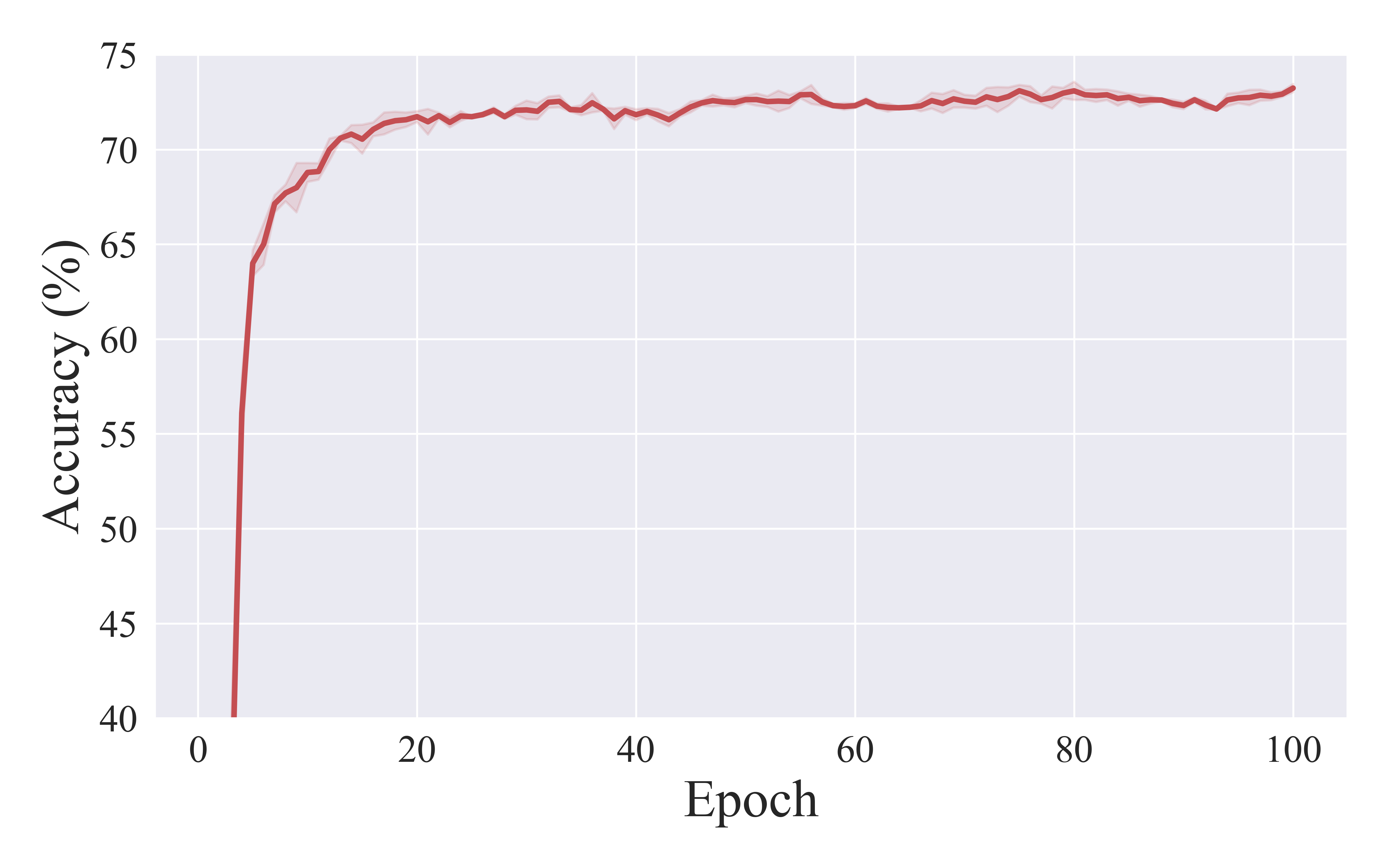
Figure ii: Convergence curve across different prompt-tuning epochs, which corresponds to Fig. i.

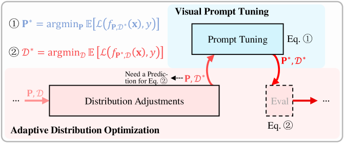
Figure iii: Proper workflow of ADO-VPT co-design framework. It is framed as an iterative process, with the VPT process nested within the ADO process.

This appendix presents further details and results that could not be included in the main paper due to space constraints. The content is organized as follows:

• § A presents detailed explanations of the related technical concepts.

• § B contains the complete results of distribution adjustments and offers an in-depth analysis of the underlying nature of ADO, which motivates the nested optimization formulation.

• § C presents attempts at adding-based adjustments, which demonstrate significant instability.

• § D explains why our proposed PR strategy relocates only a single prompt for each iteration.

• § E details the derivation of the Taylor expansion for the idleness score.

• § F provides more details of implementation.

• § G provides complete results for VTAB-1k and FGVC and presents additional experimental results.

• § H includes additional visualizations and analyses.

• § I discusses the limitations of PRO-VPT and points out the potential direction for our future work.

Appendix A Detailed Explanations of Technical Concepts

To help readers better understand the relevant technical concepts mentioned in this paper, we provide a detailed explanation of the related approaches as follows:

Vision Transformer. Given an input image $\mathbf{x}$, ViT [7, 24] first divides it into $n_{e}$ fixed-sized patches. Each patch is then embedded into $d$-dimensional latent space and combined with position encoding. The resulting set of patch embeddings is denoted as $\mathbf{E}_{0}\!=\!\{\mathbf{e}_{0j}\!\in\!\mathbb{R}^{d}\}^{n_{e}}_{j=1}$. A learnable classification token $\mathbf{x}_{0}$ is then concatenated with these embeddings, forming the input sequence $[\mathbf{x}_{0},\mathbf{E}_{0}]$. This sequence is then fed into a series of $L$ Transformer blocks $\{B_{i}\}^{L}_{i=1}$ as follows:

$$[\mathbf{x}_{i},\mathbf{E}_{i}]=B_{i}\big{(}[\mathbf{x}_{i-1},\mathbf{E}_{i-1}]\big{)},\leavevmode\nobreak\ i=1,2,\ldots,L.$$ (i)

Visual Prompt Tuning. Given a set of trainable prompt tokens $\mathbf{P}$ and the prompted backbone $f_{\mathbf{P}}$, the overall objective of VPT is to optimize these prompts for effectively adapting the PVM to downstream tasks:

$$\min_{\mathbf{P}}\leavevmode\nobreak\ \mathbb{E}_{(\mathbf{x},y)\in\mathcal{T}_{tr}}\big{[}\mathcal{L}(f_{\mathbf{P}}(\mathbf{x}),y)\big{]}.\vskip-2.87996pt$$ (ii)

This formulation specifically corresponds to Eq. (2). Depending on how the prompt set $\mathbf{P}$ is distributed across the Transformer blocks, the standard VPT [20] can be categorized into two variants, VPT-Shallow and VPT-Deep:

VPT-Shallow. The entire set of $p$ prompts, $\mathbf{P}\!=\!\{\mathbf{p}_{k}\!\in\!\mathbb{R}^{d}\}^{p}_{k=1}$, is introduced merely in the first block. The shallow-prompted model is formulated as:

$$\hskip-10.0pt[\mathbf{x}_{1},\mathbf{Z}_{1},\mathbf{E}_{1}]\! =\!B_{1}\big{(}[\mathbf{x}_{0},\mathbf{P},\mathbf{E}_{0}]\big{)},$$ (iii)

$$\hskip-10.0pt[\mathbf{x}_{i},\mathbf{Z}_{i},\mathbf{E}_{i}]\! =\!B_{i}\big{(}[\mathbf{x}_{i-1},\mathbf{Z}_{i-1},\mathbf{E}_{i-1}]\big{)},\leavevmode\nobreak\ i\!=\!2,3,\ldots,L.$$ (iv)

VPT-Deep. The prompt set $\mathbf{P}$ is uniformly distributed across all blocks, where each block $i$ is allocated a subset of $m$ prompts, $\mathbf{P}_{i}\!=\!\{\mathbf{p}_{ik}\!\in\!\mathbb{R}^{d}\}^{m}_{k=1}$, with $\mathbf{P}\!=\!\bigcup^{L}_{i=1}\mathbf{P}_{i}$. The formulation of the deep-prompted model is as follows:

$$\hskip-4.0pt[\mathbf{x}_{i},\_,\mathbf{E}_{i}]=B_{i}\big{(}[\mathbf{x}_{i-1},\mathbf{P}_{i-1},\mathbf{E}_{i-1}]\big{)},\leavevmode\nobreak\ i=1,2,\ldots,L.\hskip-3.0pt$$ (v)

where ‘$\_$’ indicates that VPT-Deep does not preserve the output corresponding to the prompt token $\mathbf{P}_{i-1}$.

Proximal Policy Optimization. PPO is an on-policy RL algorithm that can be applied to both discrete and continuous action spaces. PPO-Clip updates policies via:

$$\theta_{t+1}=\mathop{\arg\min}\limits_{\theta}\leavevmode\nobreak\ \mathbb{E}_{s,a\sim\pi_{\theta_{t}}}\big{[}L(s,a,\theta_{t},\theta)\big{]},$$ (vi)

where $\pi$ is the policy, $\theta$ is the policy parameter, and $t$ is the $t^{\text{th}}$ step. It typically takes multiple steps of SGD to optimize the objective function $L$:

$$L(s,a,\theta_{t},\theta)=$$

$$\;\min\big{(}\frac{\pi_{\theta}(a\!\mid\!s)}{\pi_{\theta_{t}}(a\!\mid\!s)}A^{\pi\theta_{t}}(s,a),\text{clip}(\frac{\pi_{\theta}(a\!\mid\!s)}{\pi_{\theta_{t}}(a\!\mid\!s)},1\!-\!\epsilon,1\!+\!\epsilon)A^{\pi\theta_{t}}(s,a)\big{)},$$ (vii)

where $A^{\pi\theta_{t}}(s,a)$ is the advantage estimator and $\epsilon$ is the clip hyper-parameter. The clip term restricts the policy change, effectively preventing the new policy from deviating significantly from the old policy [33].

Appendix B Comprehensive Analysis of the Underlying Nature behind ADO

Fig. i presents the complete results from Fig. 2. Specifically, we investigated the performance gaps from distribution adjustments applied to prompts at different epochs, both before and after prompt tuning, on VTAB-1k Natural DTD using ViT-B/16. For the adding-based adjustment, we trained with a total of 59 prompts distributed uniformly across 12 Transformer blocks, resulting in one block containing 4 prompts while the others contained 5, then added a new prompt to the block with 4 prompts. For the repositioning-based adjustment, we trained with 60 prompts allocated uniformly, and then repositioned a single prompt. For fair comparison, we averaged the results over different configurations, including variations in which block had the missing prompt and which specific prompt was repositioned.

Comparing the left and right parts of Fig. i, we find that merely adjusting the distribution without prompt tuning leads to negligible changes or even degrades performance. In contrast, implementing prompt tuning after adjusting the distribution leads to significant performance changes, with well-chosen adjustments leading to notable improvements (e.g., an increase of up to 2.2% achieved by repositioning just a single prompt). This brings us to:

Discovery 3. The effectiveness of distribution adjustments becomes apparent only after prompt tuning, suggesting that these adjustments can only be properly evaluated after tuning, thereby establishing a nested mechanism between ADO and VPT.

As demonstrated in the right portion of Fig. i, for prompts from epoch 25, we observe significant performance gains by adding a new prompt to the 10${}^{\text{th}}$ and 12${}^{\text{th}}$ blocks, as well as by repositioning one prompt to the 10${}^{\text{th}}$ and 11${}^{\text{th}}$ blocks. However, for prompts at epoch 75, the key improvements shifted to adding a prompt to the 6${}^{\text{th}}$ block and repositioning one prompt to the 6${}^{\text{th}}$ and 9${}^{\text{th}}$ blocks. This leads us to:

Discovery 2. Adjustments in prompt distribution are influenced by the updated prompts themselves, underscoring the necessity of an iterative mechanism that continuously refines the distribution over prompt updates.

Additionally, to validate that the performance improvements from applying both distribution adjustments and prompt tuning stem primarily from the distribution adjustments rather than the tuning itself, we display the corresponding accuracy curve of prompt tuning in Fig. iii. Clearly, the prompted model has already converged around epoch 20, with only slight performance fluctuations thereafter (less than 0.3%). This indicates that the performance differences observed in Fig. i (typically exceeding 0.3%) cannot be attributed solely to prompt tuning alone, but rather to the adjustments in prompt distribution.

Building upon the mechanisms described in Discoveries 2 and 3, a proper workflow for ADO and VPT should be structured as an iterative process, with VPT nested within ADO. Specifically, in each iteration, the process should first adjust the distribution to construct $\mathcal{D}^{\ast}$, followed by tuning the visual prompts to obtain $\mathbf{P}^{\ast}$. Based on $\mathcal{D}^{\ast}$ and $\mathbf{P}^{\ast}$, the distribution adjustments can be properly evaluated at the end. Fig. iii illustrates this co-design workflow for ADO and VPT. Formally, it can be expressed as a nested optimization problem, as follows:

$$\mathcal{D}^{\ast} =\mathop{\arg\min}\limits_{\mathcal{D}}\leavevmode\nobreak\ \mathbb{E}_{(\mathbf{x},y)\in\mathcal{T}_{tr}}\big{[}\mathcal{L}(f_{\mathbf{P}^{\ast},\mathcal{D}}(\mathbf{x}),y)\big{]},$$ (viii)

$$\mathbf{P}^{\ast} =\mathop{\arg\min}\limits_{\mathbf{P}}\leavevmode\nobreak\ \mathbb{E}_{(\mathbf{x},y)\in\mathcal{T}_{tr}}\big{[}\mathcal{L}(f_{\mathbf{P},\mathcal{D}^{\ast}}(\mathbf{x}),y)\big{]},$$ (ix)

where the notations $\mathbf{P}^{\ast}$ and $\mathcal{D}^{\ast}$ correspond to those depicted in Fig. iii. This formulation is applicable to various distribution adjustment strategies, including adding, repositioning, and even pruning.

Overall, the ADO problem is naturally formulated as a nested problem, grounded in its underlying mechanisms. Notably, since distribution adjustments can only be evaluated at the end, a prediction for Eq. viii is necessary for selecting appropriate adjustments. To this end, it is natural to frame ADO as a RL problem, where the reward is predicted to determine the next action, and the action’s effectiveness is evaluated afterward.

Appendix C Inferior Performance of Adding-based Adjustments

Following the nested optimization framework described in Eqs. (viii) and (ix), we have also attempted to develop an adding-based strategy for ADO. Given that framing the ADO objective as a RL problem is a suitable choice, we also address the adding-based ADO by leveraging RL, with the components of the Markov decision process specified as follows:

1) State. We utilize the current prompt distribution as the state, denoted as $s=\mathcal{D}$. After adding a new prompt and performing prompt tuning, the state transitions to $s^{\prime}$.

2) Action. Unlike prompt repositioning, which considers $L^{2}$ possible block arrangements, the adding-based ADO involves only $L$ potential adding operations. As a result, the adding-based ADO does not require simplification, and the action is straightforwardly represented as $a\in[L]$.

3) Reward. Similar to the PR strategy, the reward is formulated based on Eq. (viii) as $r\!=\!\Delta\mathcal{L}(f_{\mathbf{P},\mathcal{D}},f_{\mathbf{P}^{\prime},\mathcal{D}^{\prime}})$, where $\mathcal{D}^{\prime}$ denotes the updated prompt distribution after adding, and $\mathbf{P}^{\prime}$ represents the tuned prompts.

Similarly, we employ PPO for this RL problem to tackle the adding-based ADO objective, while adopting the overall framework illustrated in Fig. iii.

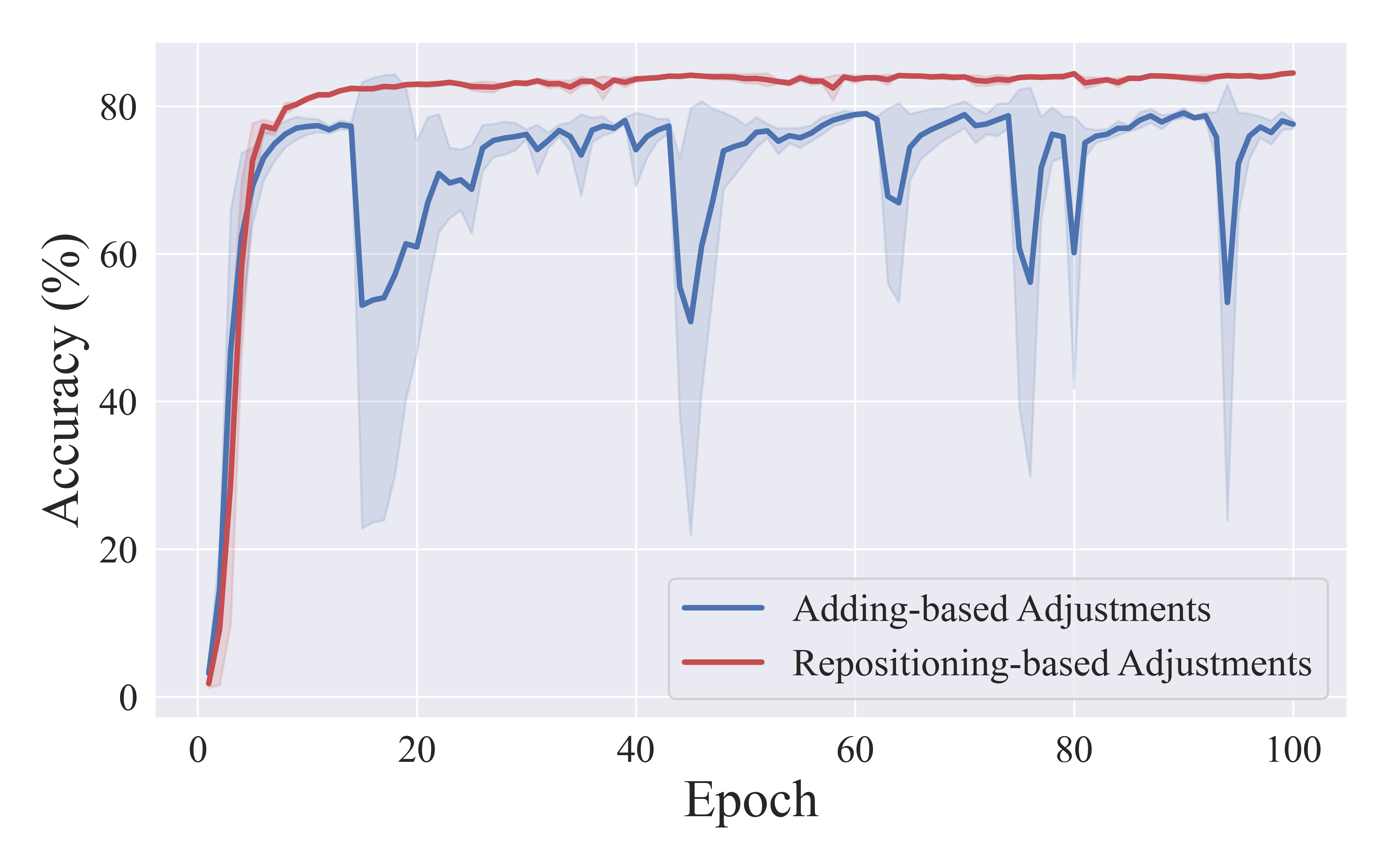
Figure iv: Convergence curves comparing adding-based and repositioning-based strategies. The adding-based strategy exhibits significantly less stability.

Fig. iv illustrates the performance comparison between the adding-based strategy and repositioning-based strategy (PRO-VPT) on the VTAB-1k Natural Cifar100 dataset. It can be clearly observed that the adding-based strategy is significantly less stable and underperforms compared to the repositioning-based approach. We attribute this discrepancy to the undertraining of newly added prompts and potential conflicts with existing ones. Consequently, our work focuses on developing the repositioning-based strategy for ADO.

Appendix D Relocating One Prompt for Each Iteration

Here, we explain why we restrict the relocation process to operate on only a single prompt for each iteration. Since we frame the allocation step as a RL problem, we need to evaluate the effectiveness of each individual allocation decision for relocated prompts. Relocating more than one prompt simultaneously would necessitate multiple reward evaluations, substantially increasing task complexity and computational overhead. Therefore, we designed to relocate only one prompt per iteration to maintain simplicity and efficiency in the allocation process.

Appendix E Derivation of the Taylor Expansion for the Idleness Score

Building upon the pruning objective in Eq. (3), the original idleness score is defined as:

$$\mathcal{I}_{k}=\Delta\mathcal{L}(f_{\mathbf{P},\mathcal{D}},f_{\mathbf{P},\mathcal{D}\mid d_{k}=0}),$$ (x)

where $d_{k}=0$ indicates that the $k^{\text{th}}$ prompt is pruned. Specifically, if the idleness score $\mathcal{I}_{k}\!>\!0$, it indicates that the loss after pruning the prompt $\mathbf{p}_{k}$, i.e. $\mathcal{L}(f_{\mathbf{P},\mathcal{D}\mid d_{k}=0}(\mathbf{x}),y)$, is lower than the loss before pruning, i.e. $\mathcal{L}(f_{\mathbf{P},\mathcal{D}}(\mathbf{x}),y)$. This suggests that $\mathbf{p}_{k}$ has a negative impact on the current model $f_{\mathbf{P},\mathcal{D}}$ and can therefore be pruned for potential relocation.

Equivalently, this equation can be expressed as:

$$\mathcal{I}_{k}=\Delta\mathcal{L}(f_{\mathbf{P},\mathcal{D}},f_{\mathbf{P}\mid\mathbf{p}_{k}=\mathbf{0},\mathcal{D}}),$$ (xi)

where $\mathbf{p}_{k}=\mathbf{0}$ represents that the $k^{\text{th}}$ prompt is a zero vector.

Let $p_{kj}\!\in\!\mathbf{p}_{k}$ denote as the prompt parameter. The difference in losses with and without the prompt parameter, i.e., the idleness score of $p_{kj}$, is given by:

$$\mathcal{I}_{kj}=\Delta\mathcal{L}(f_{\mathbf{P},\mathcal{D}},f_{\mathbf{P}\mid p_{kj}=0,\mathcal{D}}).$$ (xii)

Table i: Hyper-parameters for VPT and PRO-VPT.

	VPT	PRO-VPT
Batch size	64 ($p\!\geq$100), 128 ($p\!<$100)	64
Learning rate schedule	cosine decay	-
Optimizer	SGD
Optimizer momentum	0.9
$base\_lr$ range	{50., 25., 10., 5., 2.5, 1., 0.5, 0.25, 0.1, 0.05}
Weight decay range	{0.01, 0.001, 0.0001, 0.0}
Drop rate	0.1
Total epochs	100

Considering the entire prompt set as a concatenated vector $\mathbf{P}\!=\!\{p_{00},p_{01},\ldots,p_{Nd}\}$, we are able to approximate $\mathcal{I}_{kj}$ in the vicinity of $\mathbf{P}$ by its first-order Taylor expansion:

$$\begin{split}\widehat{\mathcal{I}}_{kj}&\approx\mathbf{g}^{T}\Big{(}\mathbf{P}-\mathbf{P}\!\mid\!p_{kj}\!=\!0\Big{)}\\ &\approx g_{kj}p_{kj},\end{split}$$ (xiii)

where $g_{kj}\!=\!\frac{\nabla\mathcal{L}}{\nabla p_{kj}}$ represents the element of the gradient $\mathbf{g}$.

For the idleness score of a prompt $\mathbf{p}_{k}\!=\!\{p_{kj}\}^{d}_{j=1}$, we can approximate it by summing the score of its individual parameters, as follows:

$$\widehat{\mathcal{I}}_{k}\approx\sum_{j=1}^{d}g_{kj}p_{kj}\approx\mathbf{g}^{T}_{k}\mathbf{p}_{k}.$$ (xiv)

To this end, we are able to efficiently approximate the idleness scores $\{\mathcal{I}_{k}\}^{N}_{k=1}$ by a single backpropagation pass, thereby avoiding the need to evaluate the idleness scores of all $N$ prompts individually.

Table ii: Specifications of the VTAB-1k datasets.

Group	Task	# Classes	Splits
			Train	Val	Test
Natural	CIFAR-100	$100$	$800$	$200$	$10\,000$
	Caltech-101	$102$			$6\,084$
	DTD	$47$			$1\,880$
	Oxford Flowers	$102$			$6\,149$
	Pets	$37$			$3\,669$
	SVHN	$10$			$26\,032$
	Sun397	$397$			$21\,750$
Specialized	Patch Camelyon	$2$	$800$	$200$	$32\,768$
	EuroSAT	$10$			$5\,400$
	RESISC45	$45$			$6\,300$
	Diabetic Retinopathy	$5$			$42\,670$
Structured	CLEVR-Count	$8$	$800$	$200$	$15\,000$
	CLEVR-Distance	$6$			$15\,000$
	DMLab	$6$			$22\,735$
	KITTI-Distance	$4$			$711$
	dSprites-Location	$16$			$73\,728$
	dSprites-Orientation	$16$			$73\,728$
	smallNORB-Azimuth	$18$			$12\,150$
	smallNORB-Elevation	$9$			$12\,150$

Table iii: Specifications of the FGVC datasets. For datasets marked with *, we follow [47] to randomly sample train and validation splits since validation sets are not available from the original datasets.

Dataset		# Classes	Splits
			Train	Val	Test
CUB-200-2011* [51]		$200$	$5\,394$	$600$	$5\,794$
NABirds* [50]		$555$	$21\,536$	$2\,393$	$6\,084$
Oxford Flowers [40]		$102$	$1\,020$	$1\,020$	$6\,149$
Stanford Dogs* [6]		$120$	$10\,800$	$1\,200$	$8\,580$
Stanford Cars* [10]		$196$	$7\,329$	$815$	$8\,041$

Table iv: Specifications of the pre-trained backbones.

Backbone	Pre-trained Strategy	Pre-trained Dataset	Param (M)	Feature dim $d$	Pre-trained Model
ViT-B/16	Supervised	ImageNet-21k	85	768	checkpoint
ViT-L/16			307	1024	checkpoint
ViT-H/14			630	1280	checkpoint
Swin-B	Supervised	ImageNet-21k	88	1024	checkpoint
ViT-B/16	MAE	ImageNet-1k	85	768	checkpoint
ViT-B/16	MoCo-v3				checkpoint

Appendix F More Implementation Details

Augmentation. Apart from data normalization, we resize the input images to 224$\times$224 pixels for VTAB-1k and apply a randomly resize crop to 224$\times$224 pixels and horizontal flipping for FGVC, as outlined in [20, 13, 47].

Training Hyper-parameters. Specific to training hyper-parameters, we largely adopt the same settings as depicted in VPT [20]. Tab. i summarizes the hyper-parameter configurations comparing the experiments of VPT and our approach. Following [20], we conduct a grid search on the validation set of each task to determine the optimal learning rate and weight decay; the learning rate is set as $base\_lr\!\times\!b/\text{256}$, where $b$ denotes the batch size and $base\_lr$ is selected from the range specified in Tab. i. Notably, PRO-VPT does not require specific-designed large learning rates as in [20]. For all experiments conducted with our implementation, the results are averaged over three random seeds.

PPO Hyper-parameters. We also detail the hyper-parameters of our PPO implementation for reproducibility. Both the actor and critic networks are two-layer MLPs with 64 hidden units per layer. The total number of parameters of the two policy networks is precisely 0.0136M. The learning rates are 0.0003 for the actor and 0.001 for the critic. Additionally, we set the discount factor to 1 and the clipping factor to 0.2.

Datasets and Pre-trained Backbones Specifications. Tabs. ii and iii present the statistics of each task in VTAB-1k and FGVC w.r.t. the number of classes and the number of images in the train, validation, and test splits. The tables are largely “borrowed” from [47]. Moreover, Tab. iv provides the details of the pre-trained backbones used in this paper, which is largely “borrowed” from [20].

Reproducibility. PRO-VPT is implemented in Pytorch and timm. Experiments are conducted on NVIDIA A30-24GB GPUs. To guarantee reproducibility, our full implementation will be publicly released.

Appendix G More Experimental Results

Table v: Comprehensive results on the VTAB-1k datasets. Performance results are reported using both ImageNet normalization ($\circ$) or Inception normalization ($\bullet$), presented in % after a complete training schedule with ViT-B/16 supervised pre-trained on ImageNet-21k. The best results of prompt-based methods and other PEFT approaches are highlighted in bold. ↯: Early-stopping based on the test set. $\dagger$: Lack of complete code or hyperparameter configurations for the method, hence results are reported as presented in the original paper. ¹Average across the average accuracies of the VTAB-1k groups, following previous work.

		Natural								Specialized					Structured
	Param (M)	Cifar100	Caltech101	DTD	Flower102	Pets	SVHN	Sun397	Group Avg.	Camelyon	EuroSAT	Resisc45	Retinopathy	Group Avg.	Clevr-Count	Clevr-Dist.	DMLab	KITTI-Dist.	dSpr-Loc.	dSpr-Ori.	sNORB-Azi.	sNORB-Ele.	Group Avg.	Global Avg.1
Full $\circ$	85.8	68.9	87.7	64.3	97.2	86.9	87.4	38.8	75.9	79.7	95.7	84.2	73.9	83.4	56.3	58.6	41.7	65.5	57.5	46.7	25.7	29.1	47.6	69.0
Full $\bullet$	85.8	73.2	92.6	70.4	97.9	86.2	90.6	39.6	78.6	87.1	96.6	87.5	74.0	86.3	66.6	61.0	49.8	79.7	82.6	51.9	33.5	37.0	57.8	74.2
Linear $\circ$	0.04	63.4	85.0	63.2	97.0	86.3	36.6	51.0	68.9	78.5	87.5	68.6	74.0	77.2	34.3	30.6	33.2	55.4	12.5	20.0	9.6	19.2	26.9	57.7
Linear $\bullet$	0.04	78.1	88.1	69.0	99.1	90.0	36.0	56.9	73.9	79.8	90.7	73.7	73.7	79.5	32.4	30.5	35.9	61.9	11.2	26.2	14.3	24.5	29.6	61.0
LoRA $\bullet$ [18]	0.29	83.0	91.7	71.6	99.2	90.9	83.8	56.7	82.4	86.2	95.7	83.5	71.9	84.3	77.7	62.3	49.0	80.2	82.2	51.7	31.0	47.0	60.1	75.6
FacT-TK8 $\circ$ [21]	0.05	70.3	88.7	69.8	99.0	90.4	84.2	53.5	79.4	82.8	95.6	82.8	75.7	84.2	81.1	68.0	48.0	80.5	74.6	44.0	29.2	41.1	58.3	74.0
$\text{FacT-TK}_{8}$ $\bullet$ [21]	0.05	74.9	92.7	73.7	99.1	91.3	85.5	57.7	82.1	86.8	94.9	84.1	70.9	84.2	81.9	64.1	49.2	77.2	83.8	53.1	28.2	44.7	60.3	75.5
FacT-TK≤32 $\circ$ [21]	0.10	70.6	90.6	70.8	99.1	90.7	88.6	54.1	80.6	84.8	96.2	84.5	75.7	85.3	82.6	68.2	49.8	80.7	80.8	47.4	33.2	43.0	60.7	75.6
FacT-TK≤32 $\bullet$ [21]	0.10	74.6	93.7	73.6	99.3	90.6	88.7	57.5	82.6	87.6	95.4	85.5	70.4	84.7	84.3	62.6	51.9	79.2	85.5	52.0	36.4	46.6	62.3	76.5
Consolidator $\dagger$ [15]	0.30	74.2	90.9	73.9	99.4	91.6	91.5	55.5	82.4	86.9	95.7	86.6	75.9	86.3	81.2	68.2	51.6	83.5	79.8	52.3	31.9	38.5	60.9	76.5
SSF ↯$\circ$ [31]	0.24	69.0	92.6	75.1	99.4	91.8	90.2	52.9	81.6	87.4	95.9	87.4	75.5	86.6	75.9	62.3	53.3	80.6	77.3	54.9	29.5	37.9	59.0	75.7
SSF ↯$\bullet$ [31]	0.24	61.9	92.3	73.4	99.4	92.0	90.8	52.0	80.3	86.5	95.8	87.5	72.8	85.7	77.4	57.6	53.4	77.0	78.2	54.3	30.3	36.1	58.0	74.6
SPT-Adapter ↯$\circ$ [16]	0.23	72.9	93.2	72.5	99.3	91.4	84.6	55.2	81.3	85.3	96.0	84.3	75.5	85.3	82.2	68.0	49.3	80.0	82.4	51.9	31.7	41.2	60.8	75.8
SPT-Adapter ↯$\bullet$ [16]	0.22	74.7	94.1	73.0	99.1	91.2	84.5	57.5	82.0	85.7	94.9	85.7	70.2	84.1	81.3	63.2	49.1	80.7	83.5	52.0	26.4	41.5	59.7	75.3
SPT-Adapter ↯$\circ$ [16]	0.43	72.9	93.2	72.5	99.3	91.4	88.8	55.8	82.0	86.2	96.1	85.5	75.5	85.8	83.0	68.0	51.9	81.2	82.4	51.9	31.7	41.2	61.4	76.4
SPT-Adapter ↯$\bullet$ [16]	0.43	74.9	93.2	71.6	99.2	91.1	87.9	57.2	82.2	87.0	95.4	86.5	72.4	85.3	81.1	63.2	50.3	80.2	84.4	51.4	31.5	42.2	60.5	76.0
Adapter+r=16 $\bullet$ [47]	0.35	83.7	94.2	71.5	99.3	90.6	88.2	55.8	83.3	87.5	97.0	87.4	72.9	86.2	82.9	60.9	53.7	80.8	88.4	55.2	37.3	46.9	63.3	77.6
Prompt-based Methods:
VPT-Deep $\circ$ [20]	0.60	78.8	90.8	65.8	98.0	88.3	78.1	49.6	78.5	81.8	96.1	83.4	68.4	82.4	68.5	60.0	46.5	72.8	73.6	47.9	32.9	37.8	55.0	72.0
VPT-Deep $\bullet$ [20]	0.60	83.0	93.0	71.2	99.0	91.3	84.1	56.0	82.5	84.9	96.6	82.5	74.5	84.6	77.5	58.7	49.7	79.6	86.2	56.1	37.9	50.7	62.1	76.4
NOAH ↯$\mathbin{\vphantom{\circ}\text{\ooalign{\clipbox{0 0 0 {}}{$\bullet$}\cr$\circ$\cr}}}$ [60]	0.43	69.6	92.7	70.2	99.1	90.4	86.1	53.7	80.2	84.4	95.4	83.9	75.8	84.9	82.8	68.9	49.9	81.7	81.8	48.3	32.8	44.2	61.3	75.5
SPT-Deep $\dagger$ [53]	0.22	79.3	92.6	73.2	99.5	91.0	89.1	51.2	82.3	85.4	96.8	84.9	74.8	85.5	70.3	64.8	54.2	75.2	79.3	49.5	36.5	41.5	58.9	75.6
iVPT $\dagger$ [62]	0.60	82.7	94.2	72.0	99.1	91.8	88.1	56.6	83.5	87.7	96.1	87.1	77.6	87.1	77.1	62.6	49.4	80.6	82.1	55.3	31.8	47.6	60.8	77.1
PRO-VPT (ours)	0.61	84.5	94.1	73.2	99.4	91.8	88.2	57.2	84.1	87.7	96.8	86.6	75.5	86.7	78.8	61.0	50.6	81.3	86.7	56.4	38.1	51.7	63.1	78.0

Table vi: Comprehensive results on the FGVC datasets. Performance results are reported as the highest of ImageNet normalization ($\circ$) or Inception normalization ($\bullet$), presented in % after a complete training schedule with ViT-B/16 supervised pre-trained on ImageNet-21k. The best results of prompt-based methods and other PEFT approaches are highlighted in bold. $\dagger$: Lack of complete code or hyperparameter configurations for the method, hence results are reported as presented in the original paper.

	Param (M)	CUB200	NABirds	Oxford Flowers	Stanford Dogs	Stanford Cars	Global Avg.
Full $\circ$	86.0	87.3	82.7	98.8	89.4	84.5	88.5
Full $\bullet$	86.0	88.0	81.5	99.2	85.6	90.6	89.0
Linear $\circ$	0.18	85.3	75.9	97.9	86.2	51.3	79.3
Linear $\bullet$	0.18	88.9	81.8	99.5	92.6	52.8	83.1
SSF $\circ$ [31]	0.39	89.5	85.7	99.6	89.6	89.2	90.7
SSF $\bullet$ [31]	0.39	88.9	85.0	99.6	88.9	88.9	90.3
SPT-Adapter $\dagger$ [16]	0.40	89.1	83.3	99.2	91.1	86.2	89.8
SPT-LoRA $\dagger$ [16]	0.52	88.6	83.4	99.5	91.4	87.3	90.1
Adapter+ $\bullet$ [47]	0.34	90.4	85.0	99.7	92.6	89.1	91.4
Prompt-based Methods:
VPT-Deep $\circ$ [20]	0.85	88.5	84.2	99.0	90.2	83.6	89.1
VPT-Deep $\bullet$ [20]	0.85	90.1	83.3	99.6	90.3	85.0	89.7
SPT-Deep $\dagger$ [53]	0.36	90.6	87.6	99.8	89.8	89.2	91.4
iVPT $\dagger$ [62]	0.41	89.1	84.5	99.5	90.8	85.6	89.9
PRO-VPT (ours)	0.86	90.6	86.7	99.7	91.8	89.6	91.7

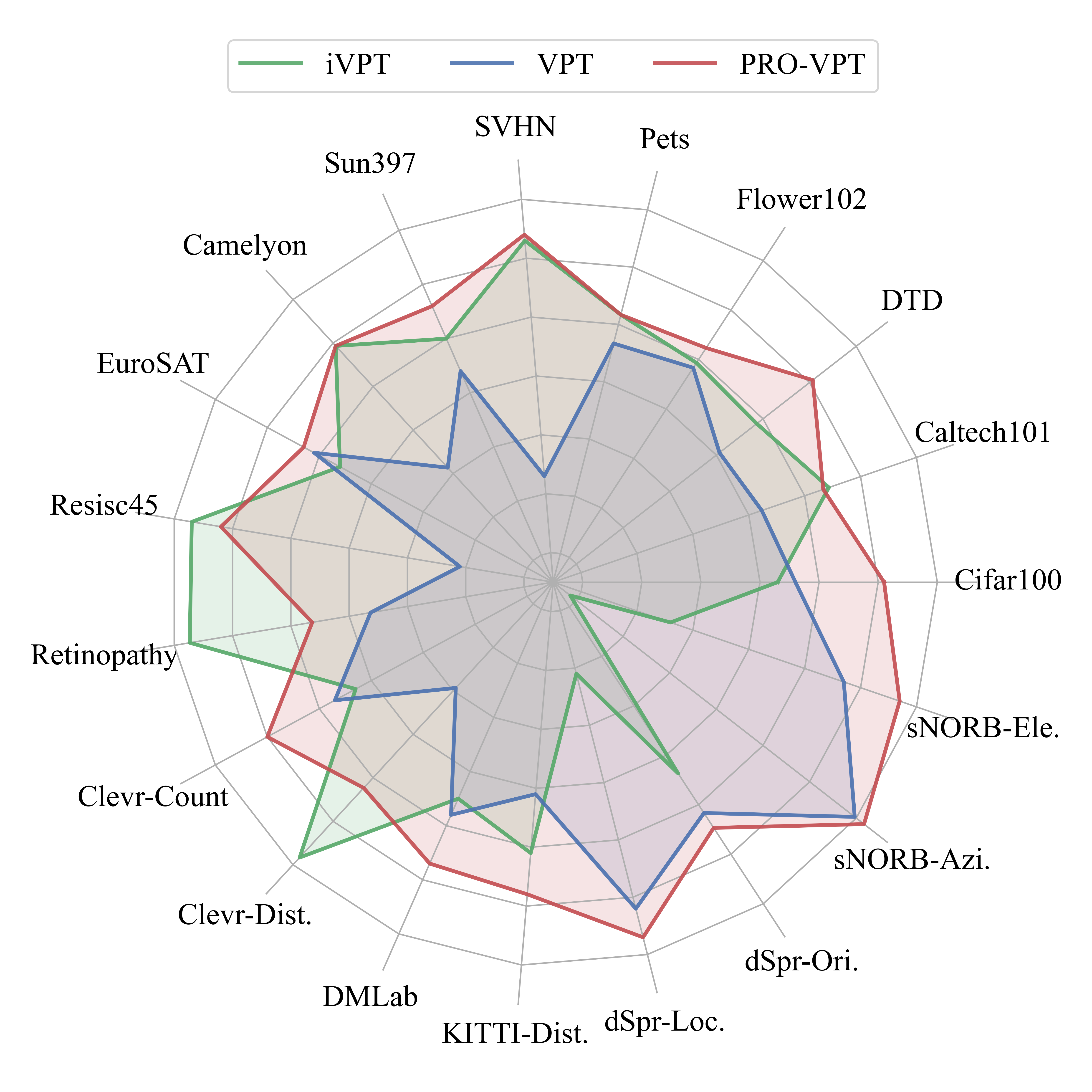
Figure v: Comparison of prior state-of-the-art (iVPT), baseline (VPT), and our method (PRO-VPT). Our approach subsumes two representative methods.

Complete Results for VTAB-1k. Tab. v presents comprehensive results for VTAB-1k, using both ImageNet and Inception normalizations. Although several of the best pre-task results from other PEFT methods differ and exceed those listed in Tab. 1, PRO-VPT remains highly competitive, achieving a state-of-the-art average accuracy of 78.0% among all evaluated methods.

Fig. v illustrates a comparison of prompt-based methods, including the previous state-of-the-art (iVPT), the baseline (VPT), and our proposal (PRO-VPT). All scores were normalized by $x_{\text{norm}}\!=\!x\!-\!x_{\text{mean}}$. It is evident that PRO-VPT outperforms both current leading methods, establishing a new state-of-the-art performance for prompt-based techniques.

Complete Results for FGVC. Tab. vi presents comprehensive results for FGVC, utilizing both ImageNet and Inception normalizations. The best pre-task results remain consistent with those in Tab. 2, and PRO-VPT demonstrates superior performance on large-scale fine-grained datasets.

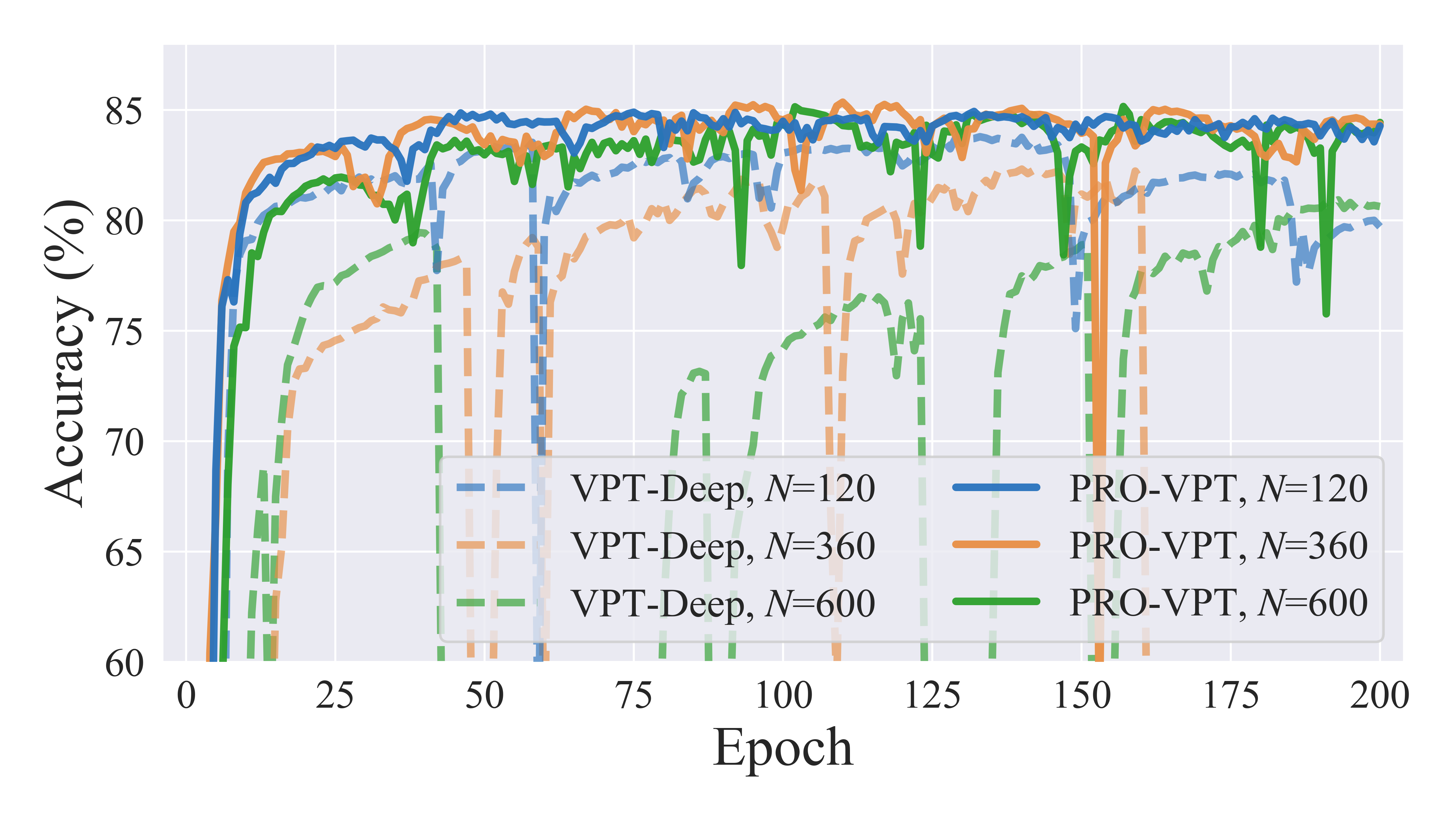
Figure vi: Convergence curves comparing VPT and PRO-VPT with varying numbers of prompts. PRO-VPT exhibits superior robustness.

Convergence Curves with Different Prompt Numbers. Fig. vi illustrates the convergence curves under varying total numbers of prompts on VTAB-1k Natural Cifar100, with training extended to 200 epochs. Notably, VPT exhibits high sensitivity to the number of prompts, as discussed in [53, 19]. An improper prompt number can lead to significant instability during convergence and result in inferior performance. In contrast, PRO-VPT demonstrates remarkable robustness to variations in prompt quantity. Although it is slightly affected during the initial convergence phase, our method ultimately converges to consistent performance. This suggests that learning the optimal distribution enables a more nuanced calibration of tuning intensity at each block, thereby enhancing robustness.

Table vii: Generalizability study on detection and segmentation tasks. Results are presented on two instances: COCO val2017 and ADE20k.

	COCO with Mask R-CNN						ADE20k with SETR
	APb	AP${}^{b}_{\text{50}}$	AP${}^{b}_{\text{75}}$	APm	AP${}^{m}_{\text{50}}$	AP${}^{m}_{\text{75}}$	mIoU-SS	mIoU-MS
VPT-Deep	33.8	57.6	35.3	32.5	54.5	33.9	39.1	40.1
PRO-VPT	34.6	58.6	36.1	33.4	55.5	34.7	40.0	41.0

• AP^b and AP^m are the average precision for objective detection and instance segmentation.

• mIoU-SS and mIoU-MS are single- and multi-scale inference of semantic segmentation.

Generalizability Study on Detection and Segmentation Tasks. We also conduct experiments on a broader range of downstream tasks, including object detection, instance segmentation, and semantic segmentation. Specifically, we evaluate object detection and instance segmentation on the COCO dataset, using Mask R-CNN with a Swin-T backbone pre-trained on ImageNet-1k. For semantic segmentation, we use the ADE20k dataset and adopt SETR-PUP with a ViT-B/16 backbone pre-trained on ImageNet-21k. As shown in Tab. vii, the results demonstrate that PRO-VPT consistently outperforms VPT across both detection and segmentation tasks, highlighting its superior generalizability.

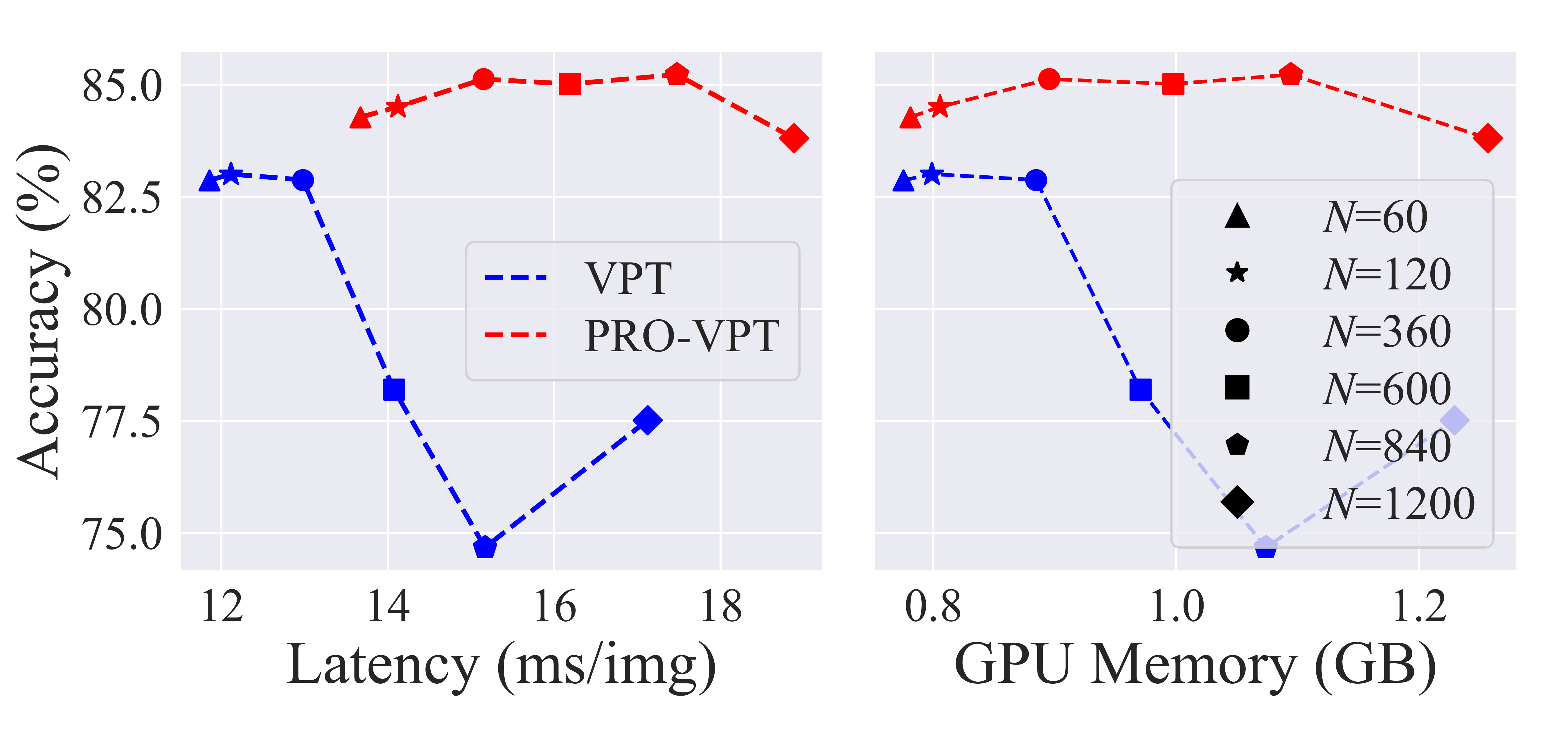
Figure vii: Cost comparisons with different prompt numbers. We report the latency (ms/img) and the peak memory usage (GB). The increased training time associated with PRO-VPT is justified by the considerable enhancements it provides in both performance and robustness.

Cost Analysis. As detailed in § 3, estimating the expected objectives effectively avoids additional computation, thereby significantly enhancing the efficiency of our method. In particular, the extra training cost of our method primarily stems from the computation of policy networks in PPO. However, since the policy networks are merely lightweight MLPs, this additional cost is relatively low. Specifically on VTAB-1k, the average latency for VPT and PRO-VPT is 13.37 ms/img and 15.55 ms/img (1.16$\mathbf{\times}$). Furthermore, we evaluate latency and GPU usage with varying prompt numbers on VTAB-1k Natural Cifar100 in Fig. vii. Although PRO-VPT does introduce some extra training time, the performance and robustness improvements justify this cost, and the increase in GPU memory usage is marginal.

Appendix H Visualization and Analysis

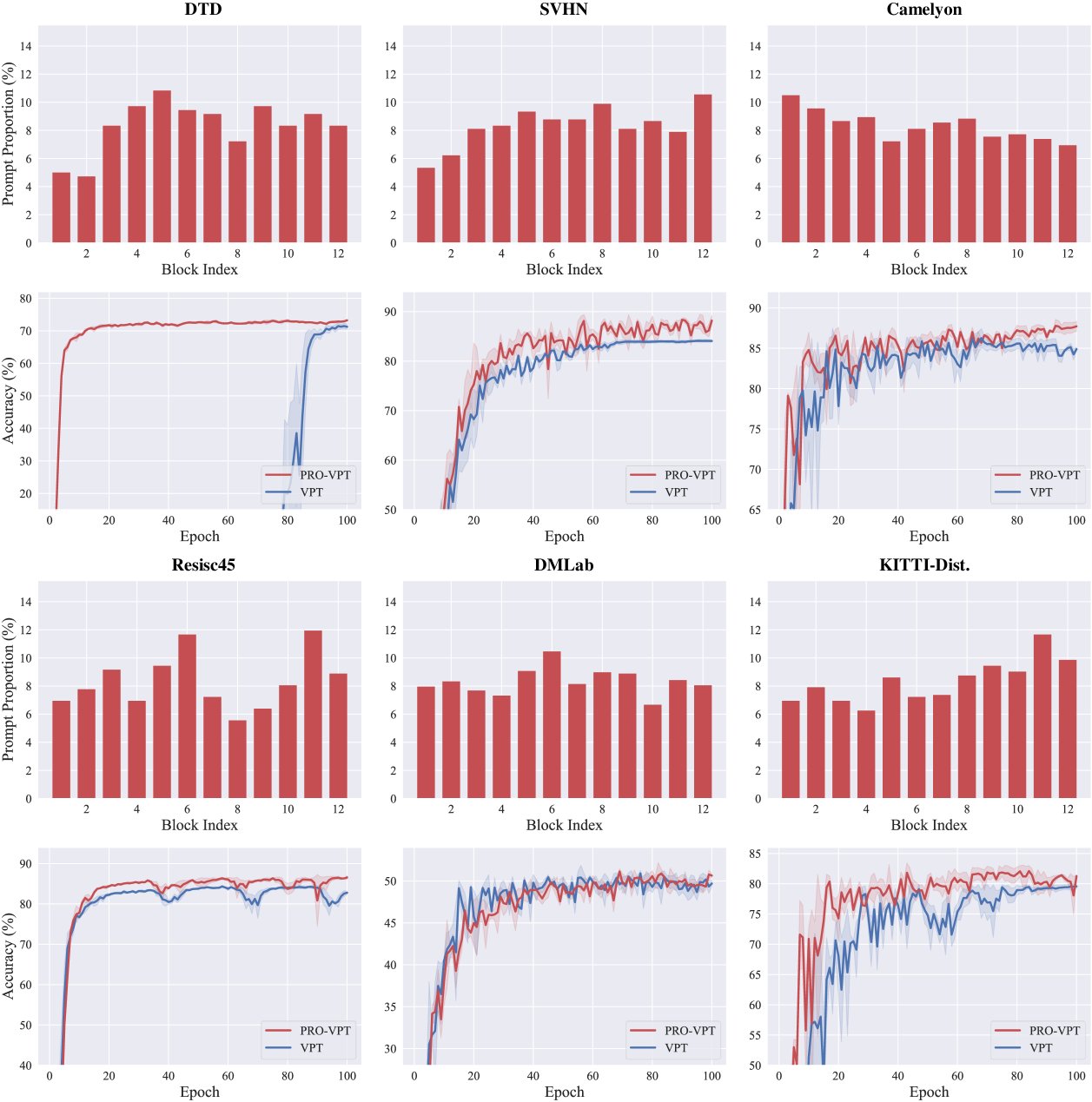
Figure viii: Visualization of the prompt distributions learned by PRO-VPT and the accuracy curves compared to VPT on the VTAB-1k datasets: Natural DTD, SVHN; Specialized Camelyon, Resisc45; and Structured DMLab, KITTI-Dist.

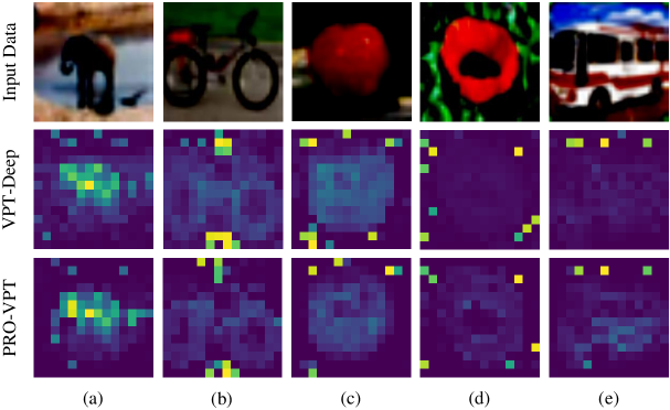
Figure ix: Visualization of attention maps. PRO-VPT exhibits more focused and precise attention with fewer artifacts.

Learned Distributions and Accuracy Curves. Fig. viii illustrates the learned distributions in PRO-VPT as well as the accuracy curves in comparison to VPT, based on 100 training epochs. Empirical results from more datasets further reinforce that the prompting importance for each block is inherently task-dependent. Moreover, the comparison of accuracy curves between PRO-VPT and VPT, particularly on the SVHN, Camelyon, and Resisc45 datasets, reveals that PRO-VPT still exhibits an upward trend in accuracy during the late training stages. This highlights the effectiveness of learning the optimal distribution for visual prompts, which unlocks their full potential and maximizes task performance.

Attention Maps. We also visualize the attention maps between [CLS] and image patches on VTAB-1k Natural Cifar100. As shown in Figs. ix(a)-(c), while VPT successfully focuses on the object, its attention exhibits significant artifacts [4] and, more critically, remains scattered. For example, in Fig. ix(a), VPT shows certain attention on the lake, which is actually part of the background. In contrast, PRO-VPT demonstrates more focused and accurate attention with fewer artifacts. Furthermore, as illustrated in Figs. ix(d) and (e), VPT appears to struggle with effectively concentrating on the object, whereas PRO-VPT maintains its ability to focus on the object.

Appendix I Limitation and Future Work

Despite demonstrating promising performance and enhanced robustness, our approach still has certain limitations. First, as noted in [53, 19], prompt-based methods are significantly sensitive to the number of prompts per block. Although our method improves robustness and mitigates this issue to some extent (see § 4.5), there is still room for further refinement. In particular, while PRO-VPT maintains robust performance within a certain range (e.g., 10-50 initialized prompts per block as in Fig. vi), its performance still deteriorates when the number of prompts deviates significantly from the optimal value. Consequently, our method still employs the optimal number of prompts per task from [20], resulting in relatively high parameter counts akin to VPT’s. Second, the constraint of relocating one prompt per iteration (see § D) restricts our method to relocating only limited prompts within certain epochs. This particularly affects tasks requiring high prompt numbers, hindering PRO-VPT’s ability to learn optimal distributions. For instance, the changes from initial uniform to learned prompt distributions are less pronounced for Camelyon and DMLab as shown in Fig. viii, which require 100 initialized prompts per block, compared to other tasks. Nevertheless, it is worth noting that PRO-VPT still delivers considerable performance enhancements on these datasets. Addressing these limitations would further enhance the efficiency and applicability of our approach in diverse computer vision tasks.

Moreover, while this paper focuses on calibrating the distribution of prompts, the PRO-VPT system is applicable to most block-wise PEFT approaches, e.g., adjusting the pre-block dimension of subspaces (i.e., the rank distribution) in adapter-based methods. An essential future direction deserving of further investigation is integrating our approach with other PEFT methods, developing a universal framework for fine-grained robust PEFT.

References

- Chen et al. [2023] Aochuan Chen, Yuguang Yao, Pin-Yu Chen, Yihua Zhang, and Sijia Liu. Understanding and improving visual prompting: A label-mapping perspective. In CVPR, pages 19133–19143, 2023.
- Chen et al. [2022] Shoufa Chen, Chongjian Ge, Zhan Tong, Jiangliu Wang, Yibing Song, Jue Wang, and Ping Luo. Adaptformer: Adapting vision transformers for scalable visual recognition. In NeurIPS, pages 16664–16678, 2022.
- Chen et al. [2021] Xinlei Chen, Saining Xie, and Kaiming He. An empirical study of training self-supervised vision transformers. In CVPR, pages 9640–9649, 2021.
- Darcet et al. [2024] Timothée Darcet, Maxime Oquab, Julien Mairal, and Piotr Bojanowski. Vision transformers need registers. In ICLR, 2024.
- Das et al. [2023] Rajshekhar Das, Yonatan Dukler, Avinash Ravichandran, and Ashwin Swaminathan. Learning expressive prompting with residuals for vision transformers. In CVPR, pages 3366–3377, 2023.
- Dataset [2011] E Dataset. Novel datasets for fine-grained image categorization. In CVPR Workshop on Fine-grained Visual Classification, 2011.
- Dosovitskiy et al. [2020] Alexey Dosovitskiy, Lucas Beyer, Alexander Kolesnikov, Dirk Weissenborn, Xiaohua Zhai, Thomas Unterthiner, Mostafa Dehghani, Matthias Minderer, Georg Heigold, Sylvain Gelly, et al. An image is worth 16x16 words: Transformers for image recognition at scale. In ICLR, 2020.
- Frankle and Carbin [2019] Jonathan Frankle and Michael Carbin. The lottery ticket hypothesis: Finding sparse, trainable neural networks. In ICLR, 2019.
- Fu et al. [2024] Minghao Fu, Ke Zhu, and Jianxin Wu. Dtl: Disentangled transfer learning for visual recognition. In AAAI, pages 12082–12090, 2024.
- Gebru et al. [2017] Timnit Gebru, Jonathan Krause, Yilun Wang, Duyun Chen, Jia Deng, and Li Fei-Fei. Fine-grained car detection for visual census estimation. In AAAI, 2017.
- Gouk et al. [2021] Henry Gouk, Timothy Hospedales, and massimiliano pontil. Distance-based regularisation of deep networks for fine-tuning. In ICLR, 2021.
- Guo et al. [2019] Yunhui Guo, Honghui Shi, Abhishek Kumar, Kristen Grauman, Tajana Rosing, and Rogerio Feris. Spottune: transfer learning through adaptive fine-tuning. In CVPR, pages 4805–4814, 2019.
- Han et al. [2023] Cheng Han, Qifan Wang, Yiming Cui, Zhiwen Cao, Wenguan Wang, Siyuan Qi, and Dongfang Liu. Eˆ 2vpt: An effective and efficient approach for visual prompt tuning. In ICCV, pages 17445–17456, 2023.
- Han et al. [2024] Cheng Han, Qifan Wang, Yiming Cui, Wenguan Wang, Lifu Huang, Siyuan Qi, and Dongfang Liu. Facing the elephant in the room: Visual prompt tuning or full finetuning? In ICLR, 2024.
- Hao et al. [2023] Tianxiang Hao, Hui Chen, Yuchen Guo, and Guiguang Ding. Consolidator: Mergable adapter with group connections for visual adaptation. In ICLR, 2023.
- He et al. [2023] Haoyu He, Jianfei Cai, Jing Zhang, Dacheng Tao, and Bohan Zhuang. Sensitivity-aware visual parameter-efficient fine-tuning. In ICCV, pages 11825–11835, 2023.
- He et al. [2022] Kaiming He, Xinlei Chen, Saining Xie, Yanghao Li, Piotr Dollár, and Ross Girshick. Masked autoencoders are scalable vision learners. In CVPR, pages 16000–16009, 2022.
- Hu et al. [2022] Edward J Hu, yelong shen, Phillip Wallis, Zeyuan Allen-Zhu, Yuanzhi Li, Shean Wang, Lu Wang, and Weizhu Chen. LoRA: Low-rank adaptation of large language models. In ICLR, 2022.
- Huang et al. [2024] Lingyun Huang, Jianxu Mao, Yaonan Wang, Junfei Yi, and Ziming Tao. Cvpt: Cross-attention help visual prompt tuning adapt visual task. arXiv preprint arXiv:2408.14961, 2024.
- Jia et al. [2022] Menglin Jia, Luming Tang, Bor-Chun Chen, Claire Cardie, Serge Belongie, Bharath Hariharan, and Ser-Nam Lim. Visual prompt tuning. In ECCV, pages 709–727, 2022.
- Jie and Deng [2023] Shibo Jie and Zhi-Hong Deng. Fact: Factor-tuning for lightweight adaptation on vision transformer. In AAAI, pages 1060–1068, 2023.
- Kaelbling et al. [1996] Leslie Pack Kaelbling, Michael L Littman, and Andrew W Moore. Reinforcement learning: A survey. Journal of Artificial Intelligence Research, 4:237–285, 1996.
- Kaplun et al. [2023] Gal Kaplun, Andrey Gurevich, Tal Swisa, Mazor David, Shai Shalev-Shwartz, and Eran Malach. Less is more: Selective layer finetuning with subtuning. arXiv preprint arXiv:2302.06354, 2023.
- Khan et al. [2022] Salman Khan, Muzammal Naseer, Munawar Hayat, Syed Waqas Zamir, Fahad Shahbaz Khan, and Mubarak Shah. Transformers in vision: A survey. CSUR, 54(10s):1–41, 2022.
- Kim et al. [2024] Youngeun Kim, Yuhang Li, Abhishek Moitra, Ruokai Yin, and Priyadarshini Panda. Do we really need a large number of visual prompts? Neural Networks, 177:106390, 2024.
- Ko et al. [2022] Yunyong Ko, Dongwon Lee, and Sang-Wook Kim. Not all layers are equal: A layer-wise adaptive approach toward large-scale dnn training. In WWW, pages 1851–1859, 2022.
- Lee et al. [2023] Yoonho Lee, Annie S Chen, Fahim Tajwar, Ananya Kumar, Huaxiu Yao, Percy Liang, and Chelsea Finn. Surgical fine-tuning improves adaptation to distribution shifts. In ICLR, 2023.
- Li et al. [2019] Xingjian Li, Haoyi Xiong, Hanchao Wang, Yuxuan Rao, Liping Liu, Zeyu Chen, and Jun Huan. Delta: Deep learning transfer using feature map with attention for convolutional networks. In ICLR, 2019.
- Li and Liang [2021] Xiang Lisa Li and Percy Liang. Prefix-tuning: Optimizing continuous prompts for generation. In ACL, pages 4582–4597, 2021.
- Li [2017] Yuxi Li. Deep reinforcement learning: An overview. arXiv preprint arXiv:1701.07274, 2017.
- Lian et al. [2022] Dongze Lian, Daquan Zhou, Jiashi Feng, and Xinchao Wang. Scaling & shifting your features: A new baseline for efficient model tuning. In NeurIPS, pages 109–123, 2022.
- Liang et al. [2022] Youwei Liang, Chongjian GE, Zhan Tong, Yibing Song, Jue Wang, and Pengtao Xie. EVit: Expediting vision transformers via token reorganizations. In ICLR, 2022.
- Lin and Beling [2021] Siyu Lin and Peter A Beling. An end-to-end optimal trade execution framework based on proximal policy optimization. In Proceedings of the twenty-ninth international conference on international joint conferences on artificial intelligence, pages 4548–4554, 2021.
- Liu et al. [2023] Pengfei Liu, Weizhe Yuan, Jinlan Fu, Zhengbao Jiang, Hiroaki Hayashi, and Graham Neubig. Pre-train, prompt, and predict: A systematic survey of prompting methods in natural language processing. CSUR, 55(9):1–35, 2023.
- Liu et al. [2022] Xiao Liu, Kaixuan Ji, Yicheng Fu, Weng Tam, Zhengxiao Du, Zhilin Yang, and Jie Tang. P-tuning: Prompt tuning can be comparable to fine-tuning across scales and tasks. In ACL, pages 61–68, 2022.
- Liu et al. [2021] Ze Liu, Yutong Lin, Yue Cao, Han Hu, Yixuan Wei, Zheng Zhang, Stephen Lin, and Baining Guo. Swin transformer: Hierarchical vision transformer using shifted windows. In ICCV, pages 10012–10022, 2021.
- Ma et al. [2022] Fang Ma, Chen Zhang, Lei Ren, Jingang Wang, Qifan Wang, Wei Wu, Xiaojun Quan, and Dawei Song. XPrompt: Exploring the extreme of prompt tuning. In EMNLP, pages 11033–11047, 2022.
- Ma et al. [2023] Jie Ma, Yalong Bai, Bineng Zhong, Wei Zhang, Ting Yao, and Tao Mei. Visualizing and understanding patch interactions in vision transformer. IEEE TNNLS, 2023.
- Malach et al. [2020] Eran Malach, Gilad Yehudai, Shai Shalev-Schwartz, and Ohad Shamir. Proving the lottery ticket hypothesis: Pruning is all you need. In ICML, pages 6682–6691, 2020.
- Nilsback and Zisserman [2008] Maria-Elena Nilsback and Andrew Zisserman. Automated flower classification over a large number of classes. In ICVGIP, pages 722–729, 2008.
- Park et al. [2024] Junyoung Park, Jin Kim, Hyeongjun Kwon, Ilhoon Yoon, and Kwanghoon Sohn. Layer-wise auto-weighting for non-stationary test-time adaptation. In WACV, pages 1414–1423, 2024.
- Ro and Choi [2021] Youngmin Ro and Jin Young Choi. Autolr: Layer-wise pruning and auto-tuning of learning rates in fine-tuning of deep networks. In AAAI, pages 2486–2494, 2021.
- Russakovsky et al. [2015] Olga Russakovsky, Jia Deng, Hao Su, Jonathan Krause, Sanjeev Satheesh, Sean Ma, Zhiheng Huang, Andrej Karpathy, Aditya Khosla, Michael Bernstein, et al. Imagenet large scale visual recognition challenge. IJCV, 115:211–252, 2015.
- Schulman et al. [2017] John Schulman, Filip Wolski, Prafulla Dhariwal, Alec Radford, and Oleg Klimov. Proximal policy optimization algorithms. arXiv preprint arXiv:1707.06347, 2017.
- Shen et al. [2021] Zhiqiang Shen, Zechun Liu, Jie Qin, Marios Savvides, and Kwang-Ting Cheng. Partial is better than all: Revisiting fine-tuning strategy for few-shot learning. In AAAI, pages 9594–9602, 2021.
- Shi and Lipani [2024] Zhengxiang Shi and Aldo Lipani. Dept: Decomposed prompt tuning for parameter-efficient fine-tuning. In ICLR, 2024.
- Steitz and Roth [2024] Jan-Martin O Steitz and Stefan Roth. Adapters strike back. In CVPR, pages 23449–23459, 2024.
- Tian et al. [2023] Junjiao Tian, Zecheng He, Xiaoliang Dai, Chih-Yao Ma, Yen-Cheng Liu, and Zsolt Kira. Trainable projected gradient method for robust fine-tuning. In CVPR, pages 7836–7845, 2023.
- Tian et al. [2024] Junjiao Tian, Yen-Cheng Liu, James S Smith, and Zsolt Kira. Fast trainable projection for robust fine-tuning. In NeurIPS, 2024.
- Van Horn et al. [2015] Grant Van Horn, Steve Branson, Ryan Farrell, Scott Haber, Jessie Barry, Panos Ipeirotis, Pietro Perona, and Serge Belongie. Building a bird recognition app and large scale dataset with citizen scientists: The fine print in fine-grained dataset collection. In CVPR, pages 595–604, 2015.
- Wah et al. [2011] Catherine Wah, Steve Branson, Peter Welinder, Pietro Perona, and Serge Belongie. The caltech-ucsd birds-200-2011 dataset. Technical report, 2011.
- Wang et al. [2025] Shaowen Wang, Linxi Yu, and Jian Li. Lora-ga: Low-rank adaptation with gradient approximation. NeurIPS, 37:54905–54931, 2025.
- Wang et al. [2024] Yuzhu Wang, Lechao Cheng, Chaowei Fang, Dingwen Zhang, Manni Duan, and Meng Wang. Revisiting the power of prompt for visual tuning. In ICML, pages 50233–50247, 2024.
- Wanjiku et al. [2023] Raphael Ngigi Wanjiku, Lawrence Nderu, and Michael Kimwele. Dynamic fine-tuning layer selection using kullback–leibler divergence. Engineering Reports, 5(5):e12595, 2023.
- Xin et al. [2024] Yi Xin, Siqi Luo, Haodi Zhou, Junlong Du, Xiaohong Liu, Yue Fan, Qing Li, and Yuntao Du. Parameter-efficient fine-tuning for pre-trained vision models: A survey. arXiv preprint arXiv:2402.02242, 2024.
- Xin et al. [2025] Yi Xin, Siqi Luo, Xuyang Liu, Haodi Zhou, Xinyu Cheng, Christina E Lee, Junlong Du, Haozhe Wang, MingCai Chen, Ting Liu, et al. V-petl bench: A unified visual parameter-efficient transfer learning benchmark. NeurIPS, 37:80522–80535, 2025.
- Xu et al. [2024] Chen Xu, Yuhan Zhu, Haocheng Shen, Boheng Chen, Yixuan Liao, Xiaoxin Chen, and Limin Wang. Progressive visual prompt learning with contrastive feature re-formation. IJCV, pages 1–16, 2024.
- Yu et al. [2024] Bruce XB Yu, Jianlong Chang, Haixin Wang, Lingbo Liu, Shijie Wang, Zhiyu Wang, Junfan Lin, Lingxi Xie, Haojie Li, Zhouchen Lin, et al. Visual tuning. CSUR, 56(12):1–38, 2024.
- Zhai et al. [2019] Xiaohua Zhai, Joan Puigcerver, Alexander Kolesnikov, Pierre Ruyssen, Carlos Riquelme, Mario Lucic, Josip Djolonga, Andre Susano Pinto, Maxim Neumann, Alexey Dosovitskiy, et al. A large-scale study of representation learning with the visual task adaptation benchmark. arXiv preprint arXiv:1910.04867, 2019.
- Zhang et al. [2024] Yuanhan Zhang, Kaiyang Zhou, and Ziwei Liu. Neural prompt search. IEEE TPAMI, 2024.
- Zhao et al. [2024] Henry Hengyuan Zhao, Pichao Wang, Yuyang Zhao, Hao Luo, Fan Wang, and Mike Zheng Shou. Sct: A simple baseline for parameter-efficient fine-tuning via salient channels. IJCV, 132(3):731–749, 2024.
- Zhou et al. [2024] Nan Zhou, Jiaxin Chen, and Di Huang. ivpt: Improving task-relevant information sharing in visual prompt tuning by cross-layer dynamic connection. arXiv preprint arXiv:2404.05207, 2024.