AKF-LIO: LiDAR-Inertial Odometry with Gaussian Map by Adaptive Kalman Filter

Abstract

Existing LiDAR-Inertial Odometry (LIO) systems typically use sensor-specific or environment-dependent measurement covariances during state estimation, leading to laborious parameter tuning and suboptimal performance in challenging conditions (e.g., sensor degeneracy and noisy observations). Therefore, we propose an Adaptive Kalman Filter (AKF)framework that dynamically estimates time-varying noise covariances of LiDAR and Inertial Measurement Unit (IMU)measurements, enabling context-aware confidence weighting between sensors. During LiDAR degeneracy, the system prioritizes IMU data while suppressing contributions from unreliable inputs like moving objects or noisy point clouds. Furthermore, a compact Gaussian-based map representation is introduced to model environmental planarity and spatial noise. A correlated registration strategy ensures accurate plane normal estimation via pseudo-merge, even in unstructured environments like forests. Extensive experiments validate the robustness of the proposed system across diverse environments, including dynamic scenes and geometrically degraded scenarios. Our method achieves reliable localization results across all MARS-LVIG sequences and ranks 8th on the KITTI Odometry Benchmark. The code will be released at https://github.com/xpxie/AKF-LIO.git.

I Introduction

Simultaneous Localization and Mapping (SLAM)refers to the task of concurrently estimating a robot’s state (e.g., position and orientation) and reconstructing a map of the environment by probabilistically fusing multi-modal sensor data. Sensors like LiDAR, camera and Inertial Measurement Unit (IMU)are utilized in multiple ways to complement each other. LiDAR-Inertial Odometry (LIO)has emerged as a dominant approach among these methods, leveraging high-precision LiDAR ranging information and high-frequency IMU measurements for robust localization and dense mapping.

Existing LIO systems still face two critical challenges despite their widespread adoption. First, they lack a generalized framework for online noise covariance estimation. Most methods rely on static sensor noise models [1, 2] or complex sensor modeling [3], leading to over-constrained or under-constrained optimization during sensor degradation or time-varying sensor noise. This results in unreliable state estimation, particularly when high confidence is assigned to measurements from LiDAR-degenerated directions or dynamic objects. Second, geometric fidelity in LiDAR maps is compromised by inadequate map representations. Conventional point clouds tend to misclassify planar surfaces as edges due to sparsity and irregularity of LiDAR data [1, 2, 4]. While advanced representations like surfel [5] and Gaussian primitives [3, 6, 7] improve geometric modeling, their resolution remains bounded by fixed voxel sizes.

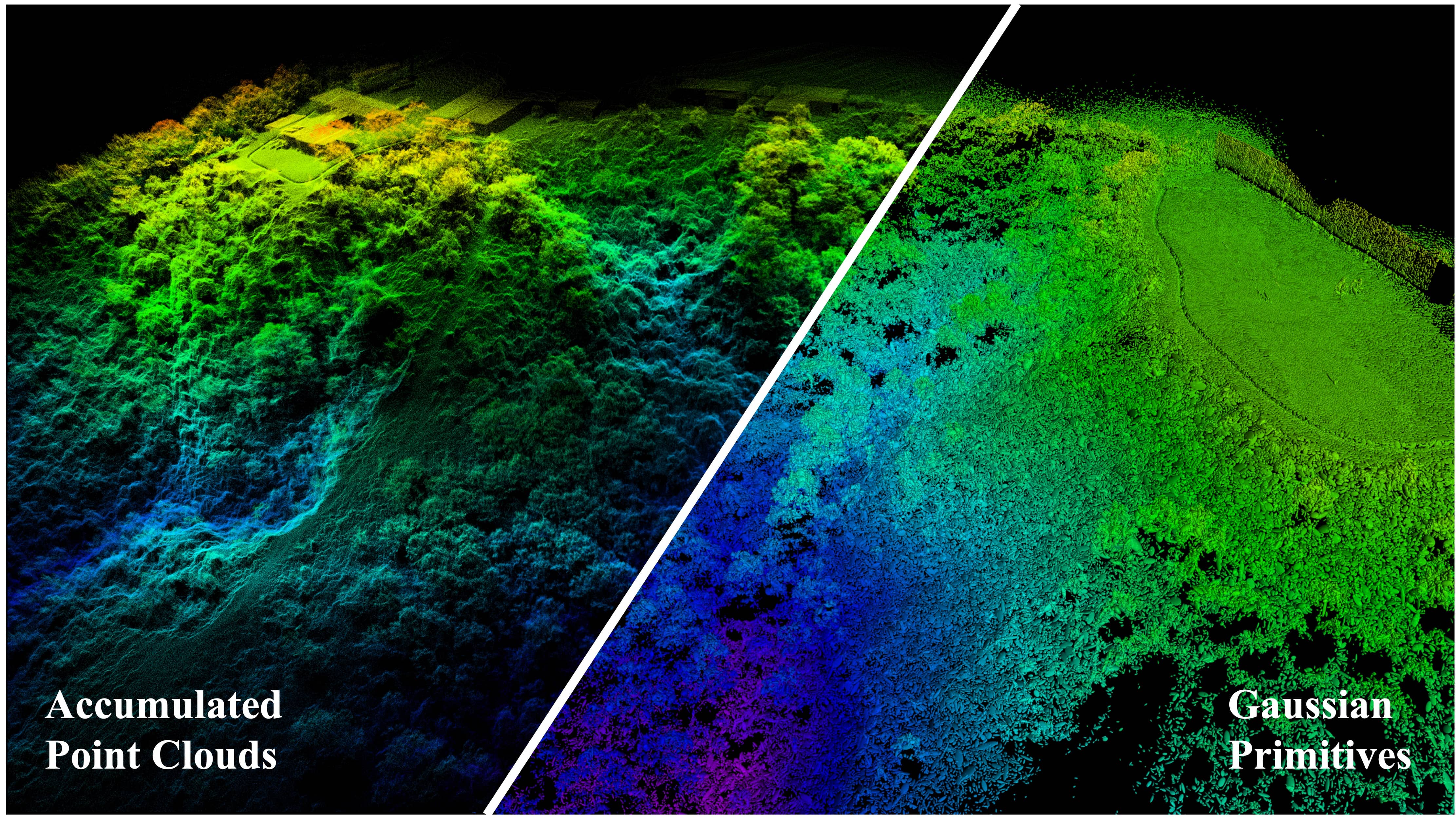
Figure 1: The mapping result of Featureless_GNSS03 sequence in MARS-LVIG dataset [8]. Left: point cloud map, right: Gaussian map, both colored by height.

To address these issues, we propose an Adaptive Kalman Filter (AKF)-based LIO framework with multi-scale Gaussian map, assuming environments consist of planar structures. The AKF dynamically estimates process and measurement noise covariances via innovation and residual terms [9]. While AKF is primarily applied to INS/GPS systems [10, 11], adapting it to LiDAR is non-trivial: verifying whether a LiDAR point belongs to a static planar surface remains challenging due to sparse and noisy neighboring points. In contrast, Gaussian distribution inherently provides continuity and outlier robustness. Therefore, our framework estimates the measurement covariance for each Gaussian map primitive by integrating its current and previous residuals. A fine-to-coarse voxelized Gaussian map preserves geometric details for small structures while aggregating large planar surfaces. Furthermore, we introduce a Gaussian-based pseudo-merge strategy to ensure accurate plane normal estimation during registration, even in unstructured environments like forests in Fig. 1. This approach guarantees that the LiDAR point to be registered lies within high-confidence regions of the pseudo-merged Gaussian. The contributions of this paper include:

1. We propose an online noise covariance estimation module for LiDAR and IMU measurements by AKF, enhancing robustness and generalizability across diverse sensor configurations and environments.

2. We propose a multi-scale Gaussian map representation constructed in a fine-to-coarse manner, paired with a correlated registration strategy, to achieve high-fidelity geometric modeling and stable plane normal estimation.

3. We verify the accuracy and robustness of our proposed method through various experiments across diverse environments, especially in dynamic and geometrically degenerated environments.

II Related work

II-A Uncertainty in LiDAR(-Inertial) Odomerty

Robust uncertainty modeling is essential for ensuring stability and reliability in LO/LIO systems, of which error sources are categorized into sensor noise and pose estimation degeneracy [12]. PUMA-LIO [13] introduces a sampling-based method to estimate noise along the plane normal direction and surface roughness. LOG-LIO2 [14] further proposes a comprehensive point uncertainty model incorporating range, bearing, incident angle and surface roughness. VoxelMap [3] extends these efforts by jointly addressing sensor noise and pose uncertainty through point-wise uncertainty aggregation into plane uncertainty.

Our method employs AKF to dynamically estimate both measurement and process covariances, enhancing resilience against sensor degradation and environmental changes. Unlike VoxelMap [3] which relies on complex physical sensor models, our method reduces reliance on prior statistical assumptions through self-adaptive covariance updates. While VoxelMap propagates pose uncertainty to all LiDAR points, we explicitly quantify constraint uncertainty per map element, enabling discrimination between well-constrained and under-constrained regions during LiDAR degeneracy. Additionally, our direct uncertainty updates on map primitives achieve faster adaptation to LiDAR degeneracy compared to VoxelMap’s point-wise uncertainty propagation.

II-B Map Representation in LiDAR(-Inertial) Odomerty

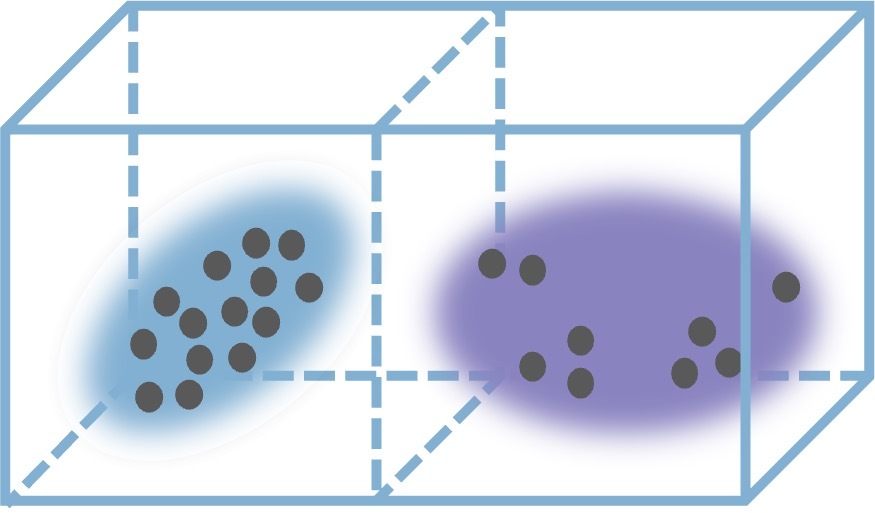
(a) Uniform voxel

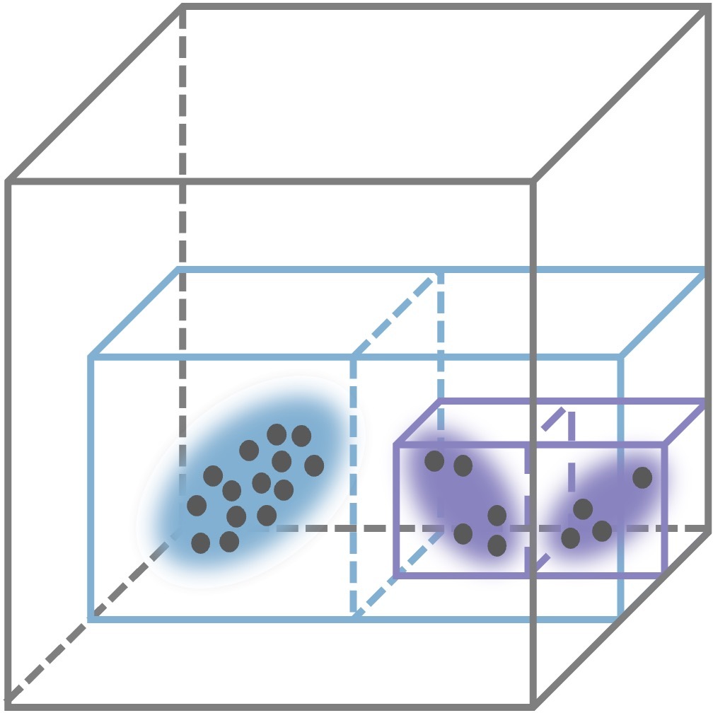
(b) Octree

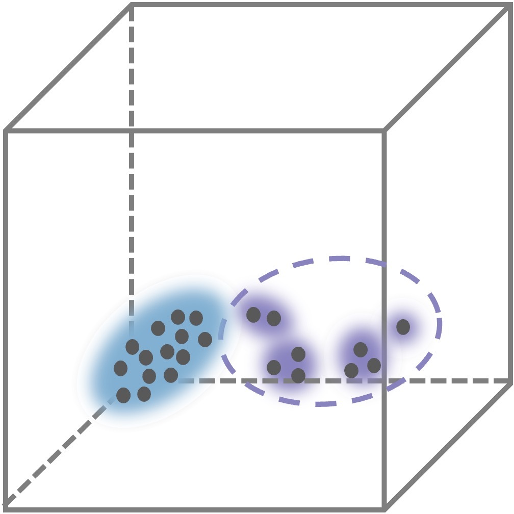
(c) Adaptive size (ours)

Figure 2: Different Gaussian-based map representations and their geometric resolution limits. (a) Uniform voxel-based Gaussian [16, 7, 6] is limited by voxel size. (b) Octree-based Gaussian [3] is limited by tree depth. (c) Gaussian with adaptive size (ours) is not limited by voxel size indicated by the small Gaussians inside the purple circle.

Point cloud is a widely adopted map representation in LO/LIO, but their computational efficiency is compromised by the massive volume of LiDAR points. To address this problem, FAST-LIO2 [15] implements a lazy update strategy via a sparse ikd-Tree for incremental maintenance, while Faster-LIO [2] enhances parallelization efficiency through voxel-based partitioning. Alternatively, Gaussian distribution has emerged as a compact representation for modeling geometric primitives (e.g., planes or edges) using Singular Value Decomposition (SVD). LiTAMIN2 [16], LIO-GVM [7], and iG-LIO [6] utilize fixed-size per-voxel Gaussians, but their geometric resolution remains bounded by predefined voxel size as illustrated in Fig. 2a. VoxelMap [3] enhances this by adopting an octree structure for adaptive voxel sizing, but it requires to store raw LiDAR points for dynamic voxel subdivision and its minimum resolution is limited by the tree depth as shown in Fig. 2b. VoxelMap++ [17] further improves accuracy and efficiency via a union-find-based plane merging strategy to construct larger planes, but it retains voxel-level resolution limits.

Our method introduces a fine-to-coarse Gaussian map representation, assuming environments comprise multi-scale planar structures. Unlike VoxelMap++ [17] which confines resolution to its minimum voxel size, our approach permits multiple Gaussians within a single voxel as demonstrated in Fig. 2c. This design preserves point-wise geometric details while aggregating large planar regions, surpassing the voxel-level resolution constraints of existing methods.

III System Overview

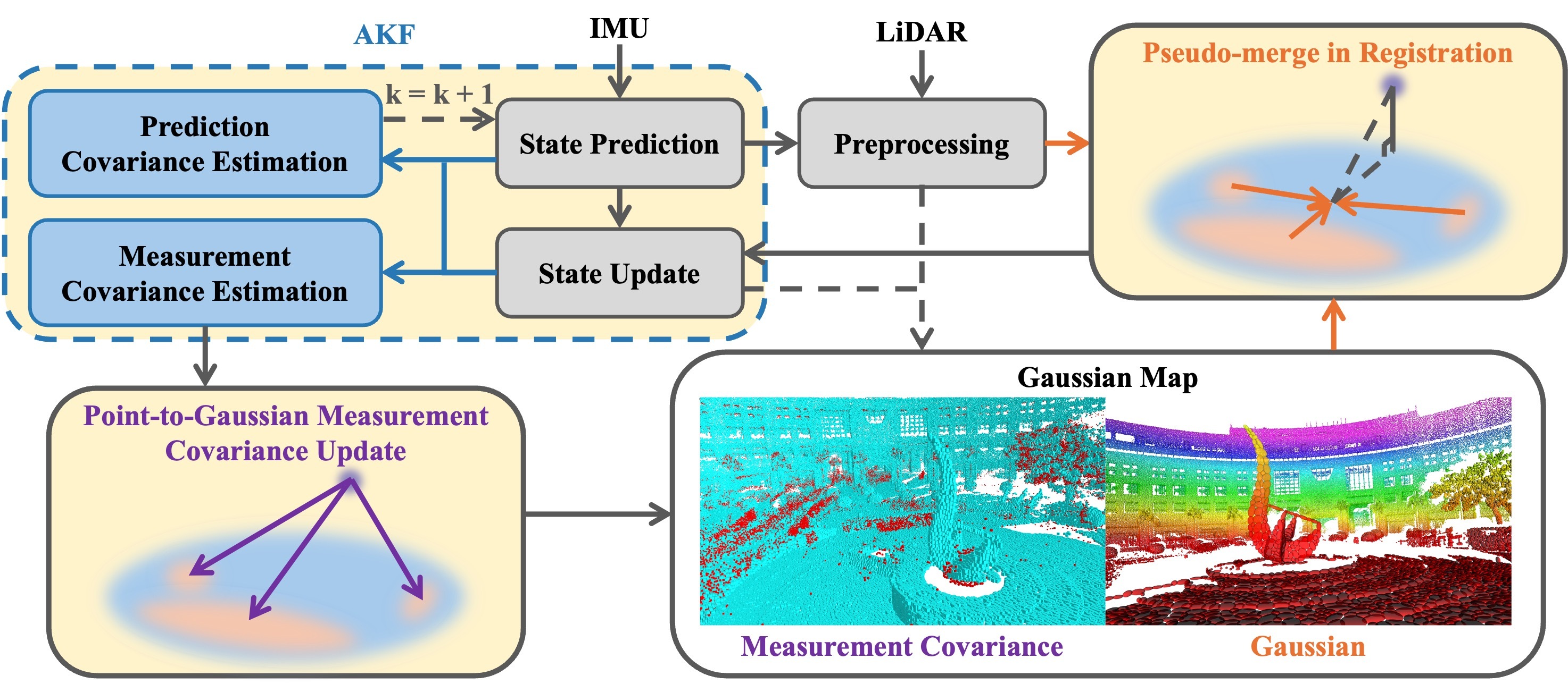
Figure 3: Framework overview of AKF-LIO. AKF estimates state by fusing IMU and LiDAR measurements with self-adjustment of prediction and measurement covariances for robustness to sensor degeneracy and environmental changes. The Gaussian map (hkust_campus_02 sequence in R3LIVE dataset[21]) maintains planar structures represented by Gaussian distribution (colored by height) and their measurement covariances (red: high covariance, blue: low covariance) which are utilized in the registration module with pseudo-merge strategy.

As illustrated in Fig. 3, the proposed system consists of three core components: an AKF, a voxel-based Gaussian map and a registration module. Synchronized IMU measurements are used for state prediction with estimated prediction covariance, enabling subsequent LiDAR scan motion compensation and state update. The undistorted point cloud after downsampling is aligned to the Gaussian map via pseudo-merge strategy weighted by dynamically estimated measurement covariances for state update. The refined state, innovation, and residual terms are leveraged to update prediction and measurement covariances to adaptively tune the filter’s parameters. Concurrently, the current LiDAR scan and its associated measurement covariances are integrated into the Gaussian map using the refined state.

TABLE I: State Notation

$\mathbf{x}$, $\widehat{\mathbf{x}}$, $\bar{\mathbf{x}}$	Ground truth, prediction and update of state $x$.
$\widetilde{\mathbf{x}}$	Error between ground truth state $\mathbf{x}$ and prediction $\widehat{\mathbf{x}}$.
$\delta{\mathbf{x}}$	Error between update state $\bar{\mathbf{x}}$ and its prediction $\widehat{\mathbf{x}}$.
$\mathbf{x}_{i}$	State $\mathbf{x}$ at the $i$th IMU sampling time.
$\mathbf{x}_{k}$	State $\mathbf{x}$ at the $k$th LiDAR scan end time.
$\mathbf{x}^{\kappa}$	State $\mathbf{x}$ at the $\kappa$th iteration.
${}^{W}(\cdot)$, ${}^{L}(\cdot)$, ${}^{I}(\cdot)$	Variables in the World, LiDAR and IMU frame.

TABLE II: Variable Definition

${{}^{W}\mathbf{R}}_{I}$, ${}^{W}\mathbf{p}_{I}$	Rotation and translation of IMU w.r.t. World.
${}^{W}\mathbf{v}_{I}$	Velocity of IMU w.r.t. World.
$\mathbf{b}_{\bm{\omega}}$, $\mathbf{b}_{\mathbf{a}}$	Bias vectors of IMU gyroscope and accelerometer.
${}^{W}\mathbf{g}$	Gravity vector w.r.t. World.
$\bm{\omega}$, ${\mathbf{a}}$	IMU gyroscope and accelerometer measurements.
$\mathbf{n}_{\bm{\omega}}$, $\mathbf{n}_{\mathbf{a}}$	Measurement noise of $\bm{\omega}$ and ${\mathbf{a}}$.
$\mathbf{n}_{\mathbf{b}\bm{\omega}}$, $\mathbf{n}_{\mathbf{b}\mathbf{a}}$	Noise of $\mathbf{b}_{\bm{\omega}}$ and $\mathbf{b}_{\mathbf{a}}$.

IV Adaptive Kalman Filter

AKF in our system is built upon the Iterated Extended Kalman Filter (iEKF)in FAST-LIO2 [1] with additional prediction and measurement covariance estimation modules to replace the original fixed IMU noise covariance and LiDAR constraint uncertainty used in FAST-LIO2. The critical notations of the state are summarized in Table I.

IV-A Problem Definition

The state $\mathbf{x}$ is defined as follows:

$$\mathbf{x} \triangleq\!\begin{bmatrix}{}^{W}{\mathbf{R}}_{I}^{T}\!&\!{}^{W}\mathbf{p}_{I}^{T}\!\!&\!{}^{W}\mathbf{v}_{I}^{T}\!&\!\mathbf{b}_{\bm{\omega}}^{T}\!&\!\!\mathbf{b}_{\mathbf{a}}^{T}\!\!&\!\!{}^{W}\mathbf{g}^{T}\end{bmatrix}^{T}\!\in\!\!\mathcal{M},$$ (1)

$$\mathcal{M} \triangleq\text{SO}(3)\times\mathbb{R}^{15},\ \dim(\mathcal{M})=18,$$

$$\mathbf{u} \triangleq\begin{bmatrix}\bm{\omega}^{T}_{m}&{\mathbf{a}}^{T}_{m}\end{bmatrix}^{T},\ \mathbf{w}\triangleq\begin{bmatrix}\mathbf{n}_{\bm{\omega}}^{T}&\mathbf{n}_{\mathbf{a}}^{T}&\mathbf{n}_{\mathbf{b}\bm{\omega}}^{T}&\mathbf{n}_{\mathbf{b}\mathbf{a}}^{T}\end{bmatrix}^{T},$$

and the involved variables are defined in Table II. iEKF aims to iteratively refine the error state $\widetilde{\mathbf{x}}$ for linearization accuracy and computational efficiency. Under the assumption that the environment consists of planar structures, the point-to-plane residual is used for the registration between the $j$th LiDAR point ${}^{L}\mathbf{p}_{j}$ with noise ${}^{L}{\mathbf{n}}_{j}$ and the map as defined in (13). Estimating $\widetilde{\mathbf{x}}_{k}^{\kappa}$ can be formulated as an MAP problem by regarding $\mathbf{x}_{k}\boxminus\widehat{\mathbf{x}}_{k}$ as its prior and combining the point-to-plane residual as the measurement model:

$$\min_{\widetilde{\mathbf{x}}_{k}^{\kappa}}\left(\|\mathbf{x}_{k}\boxminus\widehat{\mathbf{x}}_{k}\|^{2}_{\widehat{\mathbf{P}}_{k}^{-1}}+\sum\limits_{j=1}^{m}\|\mathbf{z}_{k,j}^{\kappa}+\mathbf{H}_{k,j}^{\kappa}\widetilde{\mathbf{x}}_{k}^{\kappa}\|^{2}_{\widehat{\mathbf{R}}_{k,j}^{-1}}\right),$$ (2)

where $\mathbf{H}_{k,j}^{\kappa}$ is the Jacobian of the residual w.r.t. $\widetilde{\mathbf{x}}_{k}^{\kappa}$, $\widehat{\mathbf{P}}_{k}$ is the IMU propagated state covariance, $\widehat{\mathbf{R}}_{k,j}$ is the uncertainty of the residual, and $\boxplus$ / $\boxminus$ refers to the mapping between the manifold $\mathcal{M}$ and its local tangent space $\mathbb{R}^{18}$ [18, 15].

IV-B State Prediction

From $k-1$th LiDAR scan end to $k$th LiDAR scan end time, the state is propagated using the synchronized IMU measurements. Combining the state transition function $\mathbf{f}(\mathbf{x},\mathbf{u},\mathbf{w})$ defined in FAST-LIO2 [1], state is propagated as follows using the $i$th IMU measurement $\mathbf{u}_{i}$:

$$\widehat{\mathbf{x}}_{i+1} =\widehat{\mathbf{x}}_{i}\boxplus\left(\Delta t\mathbf{f}(\widehat{\mathbf{x}}_{i},\mathbf{u}_{i},\mathbf{0})\right),\ \widehat{\mathbf{x}}_{0}=\bar{\mathbf{x}}_{k-1},$$ (3)

$$\widehat{\mathbf{P}}_{i+1} =\mathbf{F}_{\widetilde{\mathbf{x}}_{i}}\widehat{\mathbf{P}}_{i}\mathbf{F}_{\widetilde{\mathbf{x}}_{i}}^{T}+\mathbf{F}_{\mathbf{w}_{i}}\mathbf{Q}_{i}\mathbf{F}_{\mathbf{w}_{i}}^{T},\ \widehat{\mathbf{P}}_{0}=\bar{\mathbf{P}}_{k-1},$$

where $\Delta t$ denotes the IMU sampling period, $\mathbf{F}_{\widetilde{\mathbf{x}}}$ and $\mathbf{F}_{\mathbf{w}}$ are the Jacobian of $\mathbf{f}\left(\mathbf{x},\mathbf{u},\mathbf{w}\right)$ w.r.t. $\widetilde{\mathbf{x}}_{i}$ and IMU noise $\mathbf{w_{i}}$ respectively as detailed in [15, 1]. Notably, $\widehat{\mathbf{Q}}_{k,i}$ denotes the covariance of $\mathbf{w}_{i}$, and it is estimated in $(\ref{eq:pred cov estimation})$.

IV-C State Update

The MAP problem modelled in Section IV-A could be solved by iEKF as follows:

$$\begin{split}\;\mathbf{P}&=\left(\mathbf{J}^{\kappa}\right)^{-1}\widehat{\mathbf{P}}_{k}\left(\mathbf{J}^{\kappa}\right)^{-T},\\ \mathbf{K}&=\left(\left(\mathbf{H}^{\kappa}\right)^{T}{\mathbf{R}}^{-1}\mathbf{H}^{\kappa}+{\mathbf{P}}^{-1}\right)^{-1}\left(\mathbf{H}^{\kappa}\right)^{T}\mathbf{R}^{-1},\\ \widehat{\mathbf{x}}_{k}^{\kappa+1}&=\widehat{\mathbf{x}}_{k}^{\kappa}\!\boxplus\!\left(-\mathbf{K}{\mathbf{z}}_{k}^{\kappa}-(\mathbf{I}-\mathbf{K}\mathbf{H}^{\kappa})(\mathbf{J}^{\kappa})^{-1}\left(\widehat{\mathbf{x}}_{k}^{\kappa}\boxminus\widehat{\mathbf{x}}_{k}\right)\right),\end{split}$$ (4)

where $\mathbf{J}^{\kappa}$ corresponds to the Jacobian of $\left(\widehat{\mathbf{x}}_{k}^{\kappa}\boxplus\widetilde{\mathbf{x}}_{k}^{\kappa}\right)\boxminus\widehat{\mathbf{x}}_{k}$ w.r.t. $\widetilde{\mathbf{x}}_{k}^{\kappa}$, $\mathbf{K}$ means the Kalman gain, $\mathbf{H}^{\kappa}$ is the stacked form of $\mathbf{H}_{k,j}^{\kappa}$, and $\mathbf{R}$ uses the stacked $\mathbf{R}_{k,j}$ as its diagonal elements. After convergence, the final state $\bar{\mathbf{x}}_{k}$ and its covariance $\bar{\mathbf{P}}_{k}$ are updated as:

$$\begin{split}\;\bar{\mathbf{x}}_{k}&=\widehat{\mathbf{x}}_{k}^{\kappa+1},\ \bar{\mathbf{P}}_{k}=\left(\mathbf{I}-\mathbf{K}\mathbf{H}^{\kappa}\right){\mathbf{P}}.\end{split}$$ (5)

IV-D Prediction / Measurement Covariance Estimation

After state update, the prediction covariance $\bar{\mathbf{Q}}_{k}$ and the measurement covariance $\bar{\mathbf{R}}_{k,j}$ are updated, and they will be used in state prediction (3) and state update (4) of $k+1$th LiDAR scan. Based on the deduction in [10, 9], $\bar{\mathbf{Q}}_{k}$ is estimated as follows:

$$\mathbf{F}_{{\mathbf{w}},k} =\sum\limits_{i=1}^{l}\mathbf{F}_{\mathbf{w}_{i}},$$ (6)

$$\delta{\mathbf{x}_{k}} =\bar{\mathbf{x}}_{k}\boxminus\widehat{\mathbf{x}}_{k},$$

$$\bar{\mathbf{Q}}_{k} =\left(\mathbf{F}_{{\mathbf{w}},k}\right)^{-1}(\delta{\mathbf{x}_{k}}\delta{\mathbf{x}_{k}}^{T})\left(\mathbf{F}_{{\mathbf{w}},k}\right)^{-T},$$

where $l$ is the number of IMU measurements from $k-1$th LiDAR scan end to $k$th LiDAR scan end. The key insight of this estimation stems from the relationship between IMU noise and the state estimation error $\delta{\mathbf{x}_{k}}$. This error arises during the state prediction phase and is corrected through the subsequent state update process. To quantify IMU noise covariance, $\delta{\mathbf{x}_{k}}\delta{\mathbf{x}_{k}}^{T}$ is mapped back to the IMU noise space parameterized by $\mathbf{w}$ via $\left(\mathbf{F}_{{\mathbf{w}},k}\right)^{-1}$. In practice, since $\left(\mathbf{F}_{{\mathbf{w}},k}\right)^{-1}$ is non-diagonal, we compute its blockwise inversion by isolating the contributions of $\mathbf{n}_{\bm{\omega}}$, $\mathbf{n}_{\mathbf{a}}$, $\mathbf{n}_{\mathbf{b}\bm{\omega}}$ and $\mathbf{n}_{\mathbf{b}\mathbf{a}}$. Unlike prior works [10, 9] which assume ${\mathbf{F}_{{\mathbf{w}},k}}$ as an identity matrix, our method employs the accumulated ${\mathbf{F}_{{\mathbf{w}},k}}$ to preserve accuracy. During IMU propagation, $\widehat{\mathbf{Q}}_{k}$ keeps unchanged for each IMU message. To fuse with historical information $\widehat{\mathbf{Q}}_{k}$ for consistency, a forgetting factor $a$ is utilized to update $\widehat{\mathbf{Q}}_{k+1}$:

$$\widehat{\mathbf{Q}}_{k+1}=a\widehat{\mathbf{Q}}_{k}+(1-a)\bar{\mathbf{Q}}_{k}.$$ (7)

Measurement covariance $\bar{\mathbf{R}}_{k,j}$ consists of two terms. One is the residual $\bar{\mathbf{z}}_{j}$ which means the error of this constraint that cannot be mitigated after state update, the other is the posterior state covariance $\bar{\mathbf{P}}_{k}$ projected to the constraint space via $\mathbf{H}_{j}^{\kappa}$:

$$\bar{\mathbf{R}}_{k,j}=(\bar{\mathbf{z}}_{j}\bar{\mathbf{z}}_{j}^{T}+\mathbf{H}_{j}^{\kappa}\bar{\mathbf{P}}_{k}\left(\mathbf{H_{j}^{\kappa}}\right)^{T}).$$ (8)

Due to the non-repetitive scanning patterns of LiDAR, maintaing $\widehat{\mathbf{R}}_{k+1,j}$ for the LiDAR point ${}^{W}\bar{\mathbf{p}}_{k,j}$ across successive scans is challenging. Therefore, we update the measurement covariance of the map element associated with ${}^{W}\bar{\mathbf{p}}_{k,j}$ using $\bar{\mathbf{R}}_{k,j}$ as formalized in (11), and the resulting measurement covariance is utilized to compute $\widehat{\mathbf{R}}_{k+1,j}$ in (14).

$\widehat{\mathbf{Q}}_{k+1}$ is used for state prediction in the $k+1$th LiDAR scan to adjust the state estimator’s confidence between IMU and LiDAR measurements. For instance, in scenarios where LiDAR degeneracy occurs during the $k$th scan, $\widehat{\mathbf{Q}}_{k+1}$ is reduced accordingly. This adjustment prioritizes IMU measurements over LiDAR data in the $k+1$th scan to prevent ill-conditioned state estimation, as $\delta{\mathbf{x}}_{k}$ becomes negligible along the degenerated direction. During the state update phase of the $k+1$th scan, $\widehat{\mathbf{R}}_{k+1,j}$ quantifies the reliability of the point-to-plane constraint. This reliability stems from the geometric thickness of the associated planar structure and the historical usage of this plane in prior registration processes. If a map element corresponds to a dynamic object, its $\widehat{\mathbf{R}}_{k+1,j}$ increases due to the growth of $\bar{\mathbf{z}}_{j}$, thereby proportionally reducing its influence on future state estimation.

V Voxel-based Gaussian Map

A voxel-based Gaussian map is proposed to represent planar structures which is constructed by dividing the 3D space into fixed-size voxels (e.g., $0.5\text{\,}\mathrm{m}$) with each voxel containing a set of Gaussian distributions. The map is updated by integrating the LiDAR scan into the Gaussian map via incremental update, and the registration is conducted by minimizing the point-to-plane residual between the LiDAR scan and the Gaussian map with a pseudo-merge correspondence matching strategy.

V-A Gaussian Map Representation

The $m$th Gaussian map primitive ${}^{W}\mathbf{G}_{m}$ is parameterized by its mean ${}^{W}\bm{\mu}_{m}$, covariance ${}^{W}\bm{\Sigma}_{m}$, observation count $n_{m}$, the times it has been used in previous registration process $c_{m}$, and its measurement covariance $\widehat{\mathbf{R}}_{m}$. The $j$th LiDAR point in $k$th scan ${}^{W}\bar{\mathbf{p}}_{k,j}$ is initialized as an isotropic Gaussian ${}^{W}{\bar{\mathbf{G}}}_{j}$ with a fixed covariance in registration and map update.

V-B Map Update

Using the updated state $\bar{\mathbf{x}}_{k}$, ${}^{W}\bar{\mathbf{G}}_{j}$ is merged with the nearest Gaussian ${}^{W}\mathbf{G}_{m}$ in the voxel it belongs to based on the Mahalanobis distance $d_{j,m}$ between ${}^{W}\bar{\mathbf{G}}_{j}$ and ${}^{W}\mathbf{G}_{m}$:

$$e_{j,m} ={}^{W}\bar{\bm{\mu}}_{j}-{}^{W}\bm{\mu}_{m},$$ (9)

$$d_{j,m} =\left(e_{j,m}\right)^{T}\left({}^{W}\bar{\bm{\Sigma}}_{j}+{}^{W}\bm{\Sigma}_{m}\right)^{-1}{}^{W}e_{j,m}.$$

If $d_{j,m}$ satisfies $\mathcal{X}^{2}$-test with $95\%$ confidence, ${}^{W}\mathbf{G}_{m}$ is fused with ${}^{W}\bar{\mathbf{G}}_{j}$ using incremental update strategy:

$$r_{j} =\frac{n_{j}}{n_{j}+n_{m}},\ r_{m}=\frac{n_{m}}{n_{j}+n_{m}},$$ (10)

$${}^{W}\bm{\mu}_{jm} =r_{j}{}^{W}\bar{\bm{\mu}}_{j}+r_{m}{}^{W}\bm{\mu}_{m},$$

$${}^{W}\bm{\Sigma}_{m} =r_{j}\left({}^{W}\bar{\bm{\Sigma}}_{j}+{}^{W}\bar{\bm{\mu}}_{j}\left({}^{W}\bar{\bm{\mu}}_{j}\right){}^{T}\right)+$$

$$r_{m}\left({}^{W}\bm{\Sigma}_{m}+{}^{W}\bm{\mu}_{m}\left({}^{W}\bm{\mu}_{m}\right){}^{T}\right)-{}^{W}\bm{\mu}_{jm}\left({}^{W}\bm{\mu}_{jm}\right){}^{T},$$

$${}^{W}\bm{\mu}_{m} ={}^{W}\bm{\mu}_{jm},$$

$$n_{m} =n_{j}+n_{m}.$$

Conversely, if no map correspondence is found, ${}^{W}\bar{\mathbf{G}}_{j}$ is added to the voxel as a new Gaussian.

Update of $\widehat{\mathbf{R}}_{m}$ in this merging process also follows the incremental update strategy by counting $c_{m}$:

$$\widehat{\mathbf{R}}_{m} =\frac{c_{m}}{c_{m}+1}\widehat{\mathbf{R}}_{m}+\frac{1}{c_{m}+1}\bar{\mathbf{R}}_{k,j},$$ (11)

$$c_{m} =c_{m}+1,$$

where $\bar{\mathbf{R}}_{k,j}$ is computed in (8).

V-C Registration

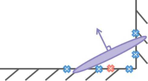
(a) Point-to-plane

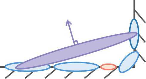
(b) VGICP

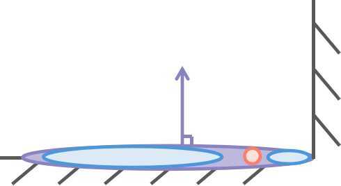
(c) Pseudo-merge (ours)

Figure 4: Different registration strategies and their plane normal estimation near the wall corner (cross: point, ellipse: Gaussian, orange: point/Gaussian in current scan, blue: point/Gaussian in the map, purple: plane for registration). (a) Point to k-nearest neighbor points [1]. (b) Distribution to k-nearest neighbor distributions [19, 7, 6]. (c) Distribution to k-nearest neighbor distributions with adaptive early termination in our method.

Algorithm 1 Correspondence Matching

1:Input: 27 neighboring voxels $\mathcal{V}$ of ${}^{W}\widehat{\mathbf{G}}_{j}^{\kappa}$

2:Output: ${}^{W}\mathbf{G}_{0m}$

3:Initialize: $\mathcal{G}\leftarrow\emptyset,{}^{W}\mathbf{G}_{0m}\leftarrow\emptyset$

4:for $v\in\mathcal{V}$ do

5:  for ${}^{W}\mathbf{G}_{m}\in v$ do

6:   $d_{j,m}^{\kappa}\leftarrow\textsc{GetDistance}({}^{W}\widehat{\mathbf{G}}_{j}^{\kappa},{}^{W}\mathbf{G}_{m})$

7:   $\mathcal{G}\leftarrow\mathcal{G}\cup\{\left(d_{j,m}^{\kappa},{}^{W}\mathbf{G}_{m}\right)\}$

8:  end for

9:end for

10:$\{\left(d_{j,0}^{\kappa},{}^{W}\mathbf{G}_{0}\right),\dots,\left(d_{j,n}^{\kappa},{}^{W}\mathbf{G}_{n}\right)\}\leftarrow\textsc{Sort}(\mathcal{G})$

11:for ${}^{W}\mathbf{G}_{m}\in\{\left(d_{j,0}^{\kappa},{}^{W}\mathbf{G}_{0}\right),\dots,\left(d_{j,n}^{\kappa},{}^{W}\mathbf{G}_{n}\right)\}$ do

12:  ${}^{W}\mathbf{G}_{0m}\leftarrow\textsc{PseudoMerge}({}^{W}\mathbf{G}_{0m},{}^{W}\mathbf{G}_{m})$

13:  if GetDistance$({}^{W}\mathbf{G}_{0m},{}^{L}\widehat{\mathbf{G}}_{j}^{\kappa})\leq d$ then break

14:  end if

15:end for

In the $\kappa$-th iteration of the state update, the Gaussian in the LiDAR frame represented as ${}^{L}{\mathbf{G}}_{j}^{\kappa}$ is first transformed to the world frame based on current state estimate $\widehat{\mathbf{x}}_{k}^{\kappa}$:

$${}^{W}\widehat{\bm{\mu}}_{j}^{\kappa} ={}^{W}\widehat{\mathbf{T}}_{L}^{\kappa}{}^{L}\bm{\mu}_{j}^{\kappa},$$ (12)

$${}^{W}\widehat{\bm{\Sigma}}_{j}^{\kappa} ={}^{W}\widehat{\mathbf{R}}_{L}^{\kappa}{}^{L}\bm{\Sigma}_{j}^{\kappa}\left({}^{W}\widehat{\mathbf{R}}_{L}^{\kappa}{}\right)^{T},$$

where ${}^{W}\widehat{\mathbf{T}}_{L}^{\kappa}$ and ${}^{W}\widehat{\mathbf{R}}_{L}^{\kappa}$ are the transformation and rotation of LiDAR w.r.t. the world frame. Under the planarity assumption, the point-to-plane residual $\mathbf{z}_{k,j}^{\kappa}$ is computed as follows:

$$\mathbf{z}_{k,j}^{\kappa}=\mathbf{u}_{0m}^{T}\left({}^{W}\widehat{\bm{\mu}}_{j}^{\kappa}-{}^{W}\bm{\mu}_{0m}\right),$$ (13)

where ${}^{W}\mathbf{G}_{0m}$ denotes the map correspondence of ${}^{W}\widehat{\mathbf{G}}_{j}^{\kappa}$ generated via the pseudo-merge strategy (Algorithm 1), and $\mathbf{u}_{0m}$ is the normal vector of ${}^{W}\mathbf{G}_{0m}$. The uncertainty $\widehat{\mathbf{R}}_{k,j}$ associated with this constraint is computed as follows:

$$c_{0m} =\sum\limits_{l=0}^{m}c_{l},$$ (14)

$$\mathbf{R}_{0m} =\frac{c_{0}}{c_{0m}}\widehat{\mathbf{R}}_{0}+\dots+\frac{c_{0}}{c_{0m}}\widehat{\mathbf{R}}_{m},$$

$$s_{0m} =\mathbf{n}_{0m}^{T}{}^{W}\bm{\Sigma}_{0m}\mathbf{n}_{0m},$$

$$\widehat{\mathbf{R}}_{k,j} =e^{-b\mathbf{R}_{0m}}s_{0m},$$

where $s_{0m}$ quantifies the squared geometric thickness of the planar structure ${}^{W}\mathbf{G}_{0m}$, $\mathbf{R}_{0m}$ corresponds to the historical uncertainty of ${}^{W}\mathbf{G}_{0m}$ being used as constraints in previous state updates, and $b$ is a positive scaling factor amplifying influence of $\mathbf{R}_{0m}$ on $\widehat{\mathbf{R}}_{k,j}$ within the exponential term. By jointly leveraging the historical reliability and current geometric fidelity of $\mathbf{R}_{0m}$, this formulation enhances the uncertainty of the constraints associated with dynamic objects. For example, if ${}^{W}\mathbf{G}_{0m}$ corresponds to a moving object, $s_{0m}$ may be small due to LiDAR point sparsity, yet $\widehat{\mathbf{R}}_{k,j}$ remains large if historical residuals of ${}^{W}\mathbf{G}_{0m}$ are persistently large as computed in (8).

The correspondence matching pipeline is formalized in Algorithm 1 and illustrated in Fig. 3. The search space is constrained to the 27 neighboring voxels of ${}^{W}\widehat{\mathbf{G}}_{j}^{\kappa}$, within which the Mahalanobis distance $d_{j,m}^{\kappa}$ between ${}^{W}\mathbf{G}_{m}$ and ${}^{W}\widehat{\mathbf{G}}_{j}^{\kappa}$ is computed as in (9). All the map Gaussians in these voxels are sorted based on $d_{j,m}^{\kappa}$ in increasing order, and we employ a pseudo-merge strategy (10) to ensure ${}^{W}\widehat{\mathbf{G}}_{j}^{\kappa}$ resides within the high-confidence region of its correspondence ${}^{W}\mathbf{G}_{0m}$ using this sorted list. Starting with the closest Gaussian ${}^{W}\mathbf{G}_{0}$ in the sorted list, it iteratively merges subsequent Gaussians until the Mahalanobis distance between ${}^{W}\mathbf{G}_{0m}$ and ${}^{W}\widehat{\mathbf{G}}_{j}^{\kappa}$ falls below a predefined threshold $d$. Once ${}^{W}\mathbf{G}_{0m}$ satisfies this criterion, the residual for this constraint is derived as in (13).

If ${}^{W}\mathbf{G}_{m}$ is pseudo-merged with ${}^{W}\mathbf{G}_{0m}$ during registration, its measurement covariance $\widehat{\mathbf{R}}_{m}$ is updated accordingly after the state update as computed in (11) and illustrated at the bottom left of Fig. 3.

As shown in Fig. 4c, the proposed pseudo-merge strategy achieves precise plane normal estimation, particularly in non-planar regions like wall corners, owing to its adaptive early termination criterion. In contrast, FAST-LIO2 [1] suffers from inaccuracies in normal estimation due to map point sparsity (Fig. 4a), while voxelized Gaussian-based methods [19, 7, 6] exhibit errors caused by over-smoothed plane merging (Fig. 4b). Notably, inaccurate plane normals degrade state estimation robustness, particularly under LiDAR degeneracy, where estimation stability is highly sensitive to noise along the unobservable direction.

VI Experiments

We conduct comprehensive evaluations of AKF-LIO across multiple benchmark datasets, including the MARS-LVIG Dataset [8], the KITTI Odometry Benchmark [20] and the R3LIVE Dataset [21]. Moreover, extensive ablation studies and performance analysis reveal the effectiveness of the proposed modules. All experiments are conducted on a desktop computer with an Intel-i9-14900KF CPU (24 cores @ 3.2 GHz) and 64GB RAM.

VI-A MARS-LVIG Dataset

TABLE III: RMSE of ATE (METERS) RESULTS ON MARS-LVIG DATASET

		HKairport			HKairport_GNSS			HKisland			HKisland_GNSS			AMtown			AMvalley			Featureless_GNSS
		01	02	03	01	02	03	01	02	03	01	02	03	01	02	03	01	02	03	01	02	03
FAST-LIO2		0.44	0.96	1.28	0.52	2.92	0.62	0.66	1.56	2.13	1.88	2.07	1.75	3.18	3.53	3.65	5.19	8.14	7.77	-	12.03	-
iG-LIO		-	-	-	-	-	-	0.28	-	-	1.83	2.03	-	1.65	-	3.54	-	-	-	-	3.45	-
R3LIVE		0.68	0.82	1.12	0.53	2.98	1.41	0.70	2.10	3.93	2.02	2.11	3.68	1.44	2.10	-	3.82	4.47	-	-	-	-
Ours		0.43	0.87	1.23	0.46	2.94	0.59	0.28	1.46	2.03	1.84	2.04	1.52	1.25	2.21	2.74	2.57	4.06	3.91	1.91	3.23	4.74

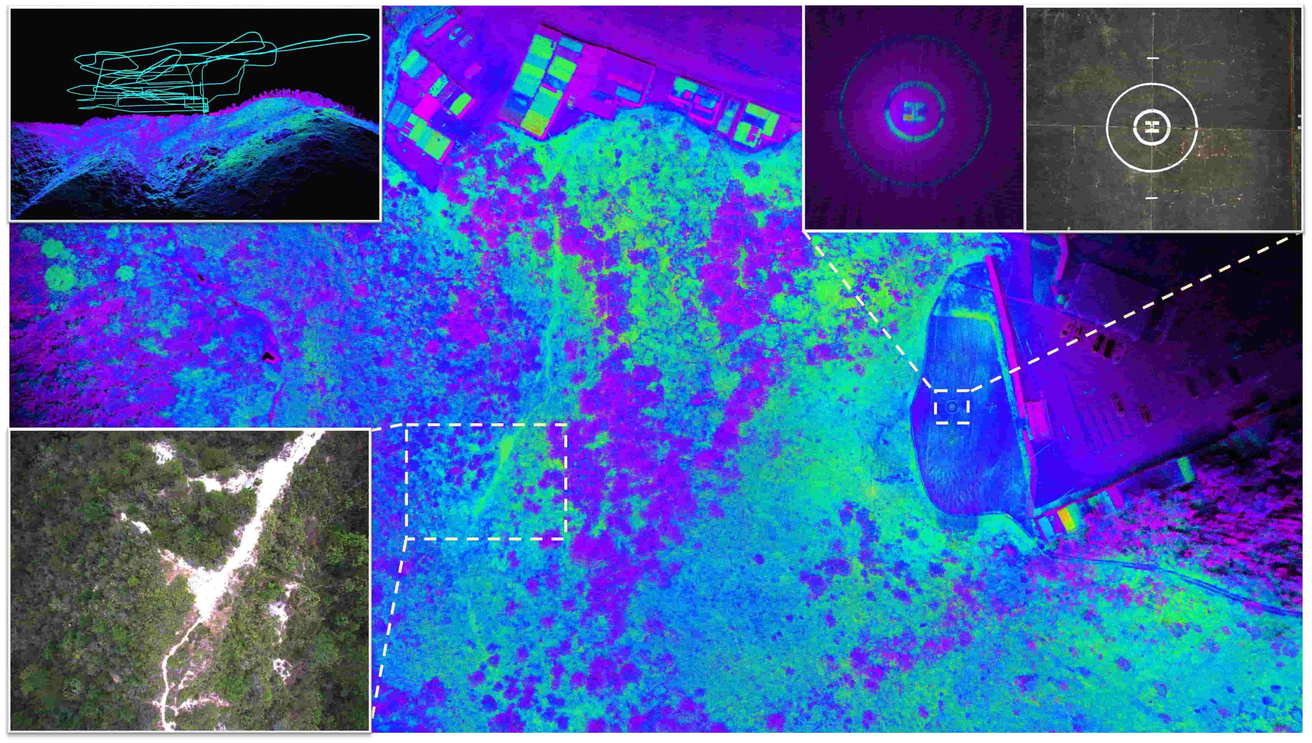
Figure 5: Accumulated LiDAR point clouds (colored by LiDAR intensity) of Featureless_GNSS03 sequence in MARS-LVIG dataset [8]. The top-left corner shows the estimated trajectory of the unmanned aerial vehicle platform used for data collection. The bottom-left depicts the camera view of the unstructureless forest environment. The top-right shows the LiDAR and camera views at the taking-off and landing position where geometry degraded because of single plane exists in the LiDAR FoV.

The MARS-LVIG dataset [8], a comprehensive multi-sensor aerial SLAM benchmark, is used to evaluate our method against FAST-LIO2 [1], iG-LIO [6], and R3LIVE [21]. FAST-LIO2 leverages a filter-based approach, fusing LiDAR and IMU measurements via an iEKF with ikd-Tree for registration. iG-LIO adopts incremental Generalized Iterative Closest Point (GICP) with surface covariance estimation akin to our method. R3LIVE integrates LiDAR, IMU and camera, employing separate subsystems for geometric mapping via LIO and texture mapping via Visual-Inertial Odometry (VIO). All methods utilize a Livox Avia LiDAR and IMU, while R3LIVE incorporates an additional RGB camera.

As outlined in Table III, FAST-LIO2 and R3LIVE achieve consistent performance across the majority of the sequences. For R3LIVE, official results are reported from the MARS-LVIG Dataset [mars_dataset] due to irreproducibility with its default parameters. In the Featureless_GNSS sequences, manual flights conducted at a low altitude of $20\text{\,}\mathrm{m}$ lead to LiDAR and visual degradations due to the sensor’s FoV being dominated by flat and textureless surfaces. Our method maintains reliable localization compared to other methods in Featureless_GNSS sequences by adaptively weighting sensor confidence via noise covariance estimation when individual sensors degrade. Our framework outperforms competitors in the AMvalley forest sequences, where FAST-LIO2 and R3LIVE exhibit over-reliance on LiDAR data, despite noise from dense tree leaves. This robustness arises from our Gaussian map representation, which inherently accommodates sensor noise through probabilistic modeling. While iG-LIO achieves competitive accuracy in stable scenarios, it fails in most sequences, likely due to its single-Gaussian-per-voxel limitation as described in Section II-B, which inadequately models complex geometries under noisy LiDAR observations. Overall, our method demonstrates consistent robustness, achieving first or second accuracy across all sequences. The qualitative result of the Featureless_GNSS03 sequence is visualized in Fig.5.

VI-B KITTI Odometry Benchmark

TABLE IV: RTE RESULTS (%) ON KITTI ODOMETRY BENCHMARK

	00	01	02	03	04	05	06	07	08	09	10	Online
KISS-ICP	0.52	0.72	0.53	0.65	0.35	0.30	0.26	0.33	0.81	0.49	0.54	0.61
CT-ICP	0.49	0.76	0.52	0.72	0.39	0.25	0.27	0.31	0.81	0.49	0.48	0.59
Traj-LO	0.50	0.81	0.52	0.67	0.40	0.25	0.27	0.30	0.81	0.45	0.55	0.58
VoxelMap	0.82	0.85	1.71	0.69	0.44	0.40	0.35	0.35	0.88	0.50	0.66	/
VoxelMap-L	0.59	0.86	0.67	0.69	0.44	0.32	0.33	0.34	0.79	0.50	0.63	/
Ours	0.49	0.65	0.50	0.66	0.37	0.26	0.29	0.32	0.80	0.46	0.54	0.59

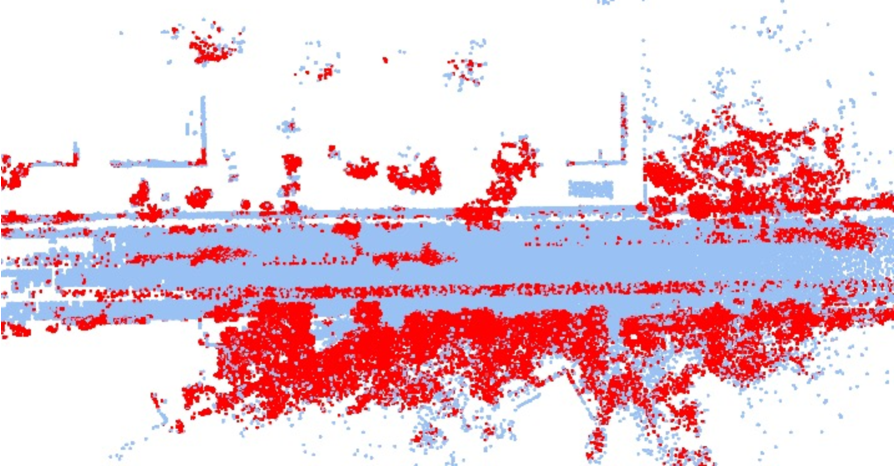
Figure 6: Visualization of the measurement covariance values stored in the Gaussian map on the KITTI 04 sequence. Large measurement covariance (red) corresponds to dynamic objects like vehicles and nonplanar shapes like corners and tree leaves, and small measurement covariance (blue) corresponds to static planar surfaces like buildings and roads.

The KITTI Odometry Benchmark [20] as a widely recognized autonomous driving dataset is employed to evaluate our method. Since IMU data is unavailable, we disable the IMU prediction module and adopt a constant velocity model. Our method is compared with LiDAR-only algorithms, including KISS-ICP [22] with point-to-point registration using adaptive correspondence thresholds, CT-ICP [23] with continuous-time intra-scan and inter-scan modeling, Traj-LO [24] with high-frequency estimation via scan segmentation, and VoxelMap [3] with octree-based voxel management with uncertainty-aware planes.

Table IV reports results using Relative Transition Error (RTE)metric. All methods achieve comparable accuracy on sequences 00-10 except VoxelMap, whose global map strategy adversely impacts RTE. Therefore, we implement VoxelMap-L, a local map variant that discards map elements older than $5\text{\,}\mathrm{s}$, to improve its RTE performance. On online benchmark sequences, Traj-LO leads with 0.58% RTE, followed closely by CT-ICP (0.59%) and our algorithm (0.59%). The online sequence results of VoxelMap are missed since they are not provided in their work. Our method currently ranks 8th on the KITTI Odometry Benchmark. The superior performance of CT-ICP and Traj-LO potentially stems from their continuous-time trajectory modeling, which aligns with RTE’s emphasis on local consistency, as proved by VoxelMap-L’s superior performance compared with original VoxelMap. Nevertheless, there are 30 parameters in CT-ICP in their configuration file, and the segment number of Traj-LO varies across different datasets. In contrast, AKF in our method integrates online covariance estimation with Gaussian map representation, enabling nearly unified parameterization across diverse datasets. As illustrated in Fig. 6, our covariance estimation module assigns larger uncertainties to dynamic objects and non-planar structures while reserving lower uncertainties for static planar surfaces, enhancing robustness in heterogeneous environments.

VI-C R3LIVE Dataset

TABLE V: END-TO-END ERRORS (METERS) ON R3LIVE DATASET

	degenerate_seq			hkust_campus
	00	01	02	00	01	02
Duration(s)	86	85	101	1073	1162	478
Length(m)	53.3	75.2	74.9	1317.2	1524.3	503.8
FAST-LIO2	8.64	6.68	49.06	5.20	0.14	0.12
R3LIVE	0.07	0.09	0.10	3.70	21.61	0.06
iG-LIO	47.41	5.35	-	2.81	3.44	0.06
Ours	0.04	13.26	0.02	0.05	2.07	0.02

We further evaluate our method in the R3LIVE [21] dataset, as it contains multiple LiDAR degenerated sequences. The groundtruth trajectory is not available and the end-to-end errors are reported in the Table V. All the methods show similar results on the non-degenerated sequences. For the degenerated_seq 00-02, FAST-LIO2 and iG-LIO quickly drift when only one plane exists in the LiDAR FoV, like facing the wall or the ground. R3LIVE shows great robustness across the three degenerated sequences by introducing camera measurements. Our method can survive in two of the degenerated sequences owing to AKF and robust registration with pseudo-merged planes. A possible reason for the failure in degenerate_seq_01 may be that the LiDAR degeneracy occurs at the beginning of the sequence where the prediction covariance estimation module fails to converge in such a short time.

VI-D Ablation Study

TABLE VI: RMSE OF ATE (METERS) RESULTS ON Field-Dynamic Sequence of ENWIDE LiDAR Inertial Dataset.

Prediction	Measurement	FAST-LIO2	Ours-iEKF	Ours-AKF
100$\mathbf{Q}$	100$\mathbf{R}$	23.78	0.18	0.20
100$\mathbf{Q}$	1$\mathbf{R}$	14.40	0.19	0.18
1$\mathbf{Q}$	100$\mathbf{R}$	45.80	89.46	0.20
1$\mathbf{Q}$	1$\mathbf{R}$	14.17	0.18	0.18
0.01$\mathbf{Q}$	0.01$\mathbf{R}$	11.82	0.18	0.19
0.01$\mathbf{Q}$	1$\mathbf{R}$	40.35	7.51	0.18
1$\mathbf{Q}$	0.01$\mathbf{R}$	0.78	0.20	0.18

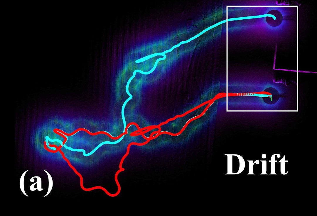
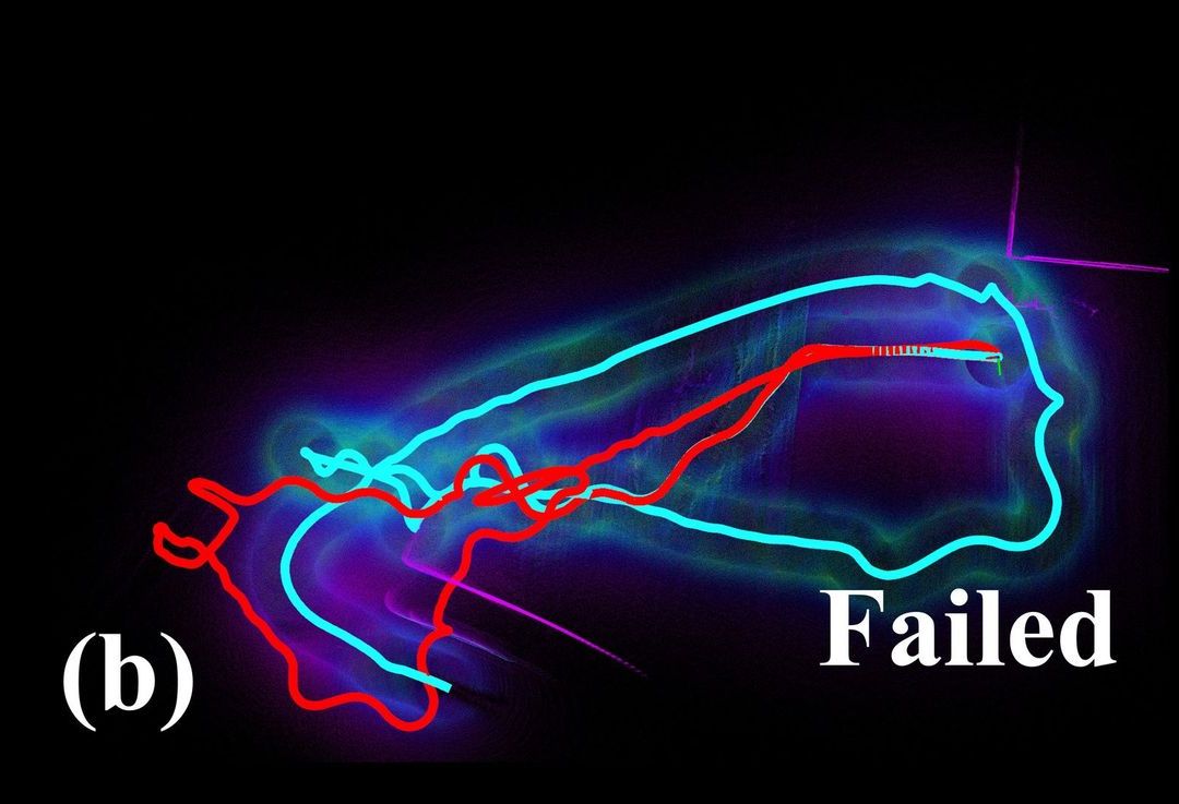
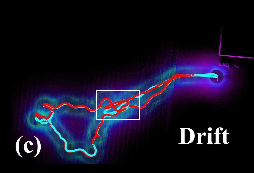
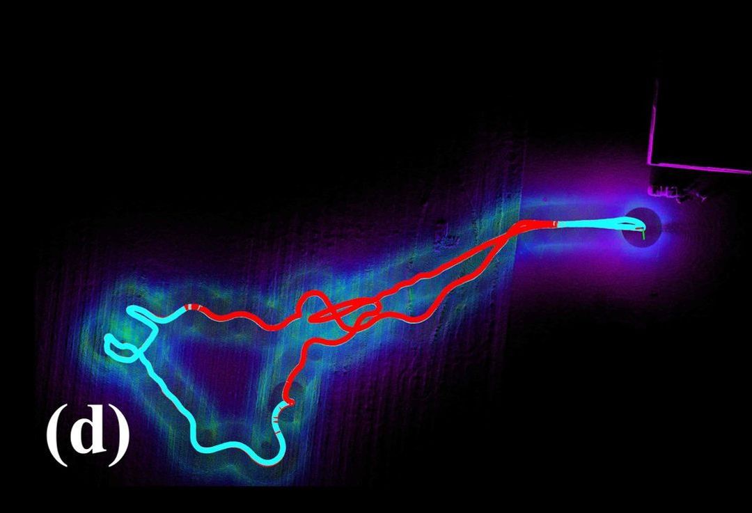
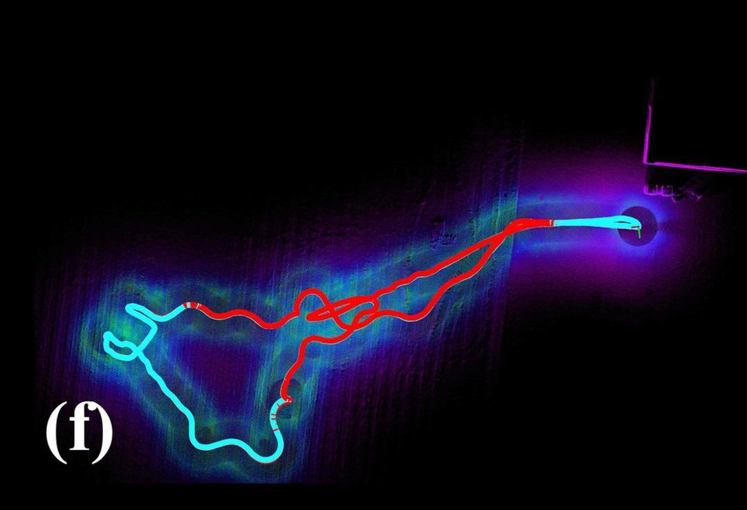
Figure 7: Qualitative results of FAST-LIO2 (a-c) and ours-AKF (d-f) on Field-Dynamic Sequence of ENWIDE LiDAR Inertial Dataset by setting different initial prediction and measurement covariances: (a) FAST-LIO2 (1$\mathbf{Q}$ and 1$\mathbf{R}$), (b) FAST-LIO2 (0.01$\mathbf{Q}$ and 1$\mathbf{R}$), (c) FAST-LIO2 (1$\mathbf{Q}$ and 0.01$\mathbf{R}$), (d) AKF-LIO (1$\mathbf{Q}$ and 1$\mathbf{R}$), (e) AKF-LIO (0.01$\mathbf{Q}$ and 1$\mathbf{R}$), (f) AKF-LIO (1$\mathbf{Q}$ and 0.01$\mathbf{R}$). The red paths show the ground truth trajectories and the cyan paths depict the estimated trajectories. The corresponding RMSE results are reported in Table VI.

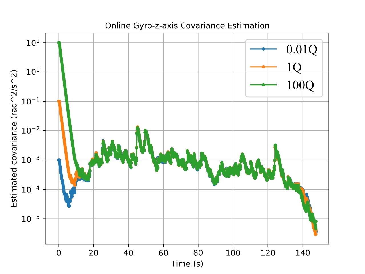
Figure 8: Online Gyro-z-axis covariance estimation with the same measurement noise (1$\mathbf{R}$) and three different prediction covariance (0.01$\mathbf{Q}$, 1$\mathbf{Q}$, 100$\mathbf{Q}$). The estimated prediction covariances quickly converge to the same level after movement at about 10 seconds.

The ablation study is conducted on the field-dynamic sequence of ENWIDE LiDAR Inertial Dataset originally used by COIN-LIO [25]. It is a short sequence containing the LiDAR-degenerated open environment, which is suitable for validating the robustness of our method in such challenging cases. Three methods are compared in this sequence, including FAST-LIO2, our method utilizing fixed covariance (Ours-iEKF) as in FAST-LIO2 and our original method (Ours-AKF). $\mathbf{Q}$ and $\mathbf{R}$ represent the default fixed prediction and measurement covariance values used in FAST-LIO2 respectively, and $\mathbf{R}$ is utilized to initialize $\widehat{\mathbf{R}}_{m}$ in Ours-AKF method. We initialize the system covariance parameter with 100$\times$, 1$\times$, 0.01$\times$ scaled $\mathbf{Q}$ and $\mathbf{R}$.

Root Mean Square Error (RMSE)of Absolute Trajectory Error (ATE)results are reported in the Table VI. FAST-LIO2 shows overconfidence on the constructed plane and drifts in most of the parameter settings, since it is geometrically under-constrained when only a single ground plane exists. For reference, COIN-LIO gets $0.581\text{\,}\mathrm{m}$ RMSE of ATE in this sequence using extra intensity channel measurement of LiDAR. Ours-iEKF, using fixed covariance parameters, performs better than FAST-LIO2 because of the better plane normal estimation of the probabilistic plane constructed by the pseudo-merge strategy. Ours-AKF with online covariance estimation shows the best robustness and achieves similar accuracy across all the varying initial settings. The results demonstrate that AKF is insensitive to the initial covariance values. Qualitative comparisons between FAST-LIO2 and ours-AKF with different parameter settings are shown in Fig. 7.

We further visualize the curves of the estimated gyroscope covariance values along its z-axis in Fig. 8 to show the quick convergence of AKF despite different initial values. As demonstrated in Fig. 8, the covariance estimation quickly decreases to a certain level since the robot stays static at the beginning of the sequence, indicating that the system has a high confidence on IMU in this period. After $10\text{\,}\mathrm{s}$, when the operator starts to move, the three estimated noises also quickly converge to the same level, followed by a drop near the sequence end when the operator goes back to the origin and remains static. This means the system has higher confidence on IMU when the operator keeps static as IMU is less noisy in such scenarios.

VI-E Performance Analysis

TABLE VII: PERFORMANCE EVALUATION ON AMtown-01 Sequence of MARS-LVIG DATASET

	FAST-LIO2	iG-LIO	VoxelMap	Ours
Time (ms)	19.51	18.20	48.14	19.05
Memory (GB)	2.20	6.67	14.15	4.32

Time and memory consumption are evaluated to show the computational efficiency of our method as illustrated in Table VII. As a result, all the methods used for comparison have real-time processing capability. Notably, VoxelMap performs the worst as it stores much more LiDAR points than the other three methods for octree subdivisions. FAST-LIO2 takes the least memory by utilizing a sparse ikd-Tree map representation[26]. Our method shows comparable processing speed and efficient memory usage by utilizing a fine-to-coarse Gaussian representation.

References

- [1] W. Xu, Y. Cai, D. He, J. Lin, and F. Zhang, “Fast-lio2: Fast direct lidar-inertial odometry,” IEEE Transactions on Robotics, vol. 38, no. 4, pp. 2053–2073, 2022.
- [2] C. Bai, T. Xiao, Y. Chen, H. Wang, F. Zhang, and X. Gao, “Faster-lio: Lightweight tightly coupled lidar-inertial odometry using parallel sparse incremental voxels,” IEEE Robotics and Automation Letters, vol. 7, no. 2, pp. 4861–4868, 2022.
- [3] C. Yuan, W. Xu, X. Liu, X. Hong, and F. Zhang, “Efficient and probabilistic adaptive voxel mapping for accurate online lidar odometry,” IEEE Robotics and Automation Letters, vol. 7, no. 3, pp. 8518–8525, 2022.
- [4] K. Chen, R. Nemiroff, and B. T. Lopez, “Direct lidar-inertial odometry: Lightweight lio with continuous-time motion correction,” in 2023 IEEE international conference on robotics and automation (ICRA). IEEE, 2023, pp. 3983–3989.
- [5] J. Behley and C. Stachniss, “Efficient surfel-based slam using 3d laser range data in urban environments.” in Robotics: Science and Systems, vol. 2018, 2018, p. 59.
- [6] Z. Chen, Y. Xu, S. Yuan, and L. Xie, “ig-lio: An incremental gicp-based tightly-coupled lidar-inertial odometry,” IEEE Robotics and Automation Letters, 2024.
- [7] X. Ji, S. Yuan, P. Yin, and L. Xie, “Lio-gvm: an accurate, tightly-coupled lidar-inertial odometry with gaussian voxel map,” IEEE Robotics and Automation Letters, 2024.
- [8] H. Li, Y. Zou, N. Chen, J. Lin, X. Liu, W. Xu, C. Zheng, R. Li, D. He, F. Kong, et al., “Mars-lvig dataset: A multi-sensor aerial robots slam dataset for lidar-visual-inertial-gnss fusion,” The International Journal of Robotics Research, p. 02783649241227968, 2024.
- [9] S. Akhlaghi, N. Zhou, and Z. Huang, “Adaptive adjustment of noise covariance in kalman filter for dynamic state estimation,” in 2017 IEEE power & energy society general meeting. IEEE, 2017, pp. 1–5.
- [10] A. Mohamed and K. Schwarz, “Adaptive kalman filtering for ins/gps,” Journal of geodesy, vol. 73, pp. 193–203, 1999.
- [11] J. Sasiadek, Q. Wang, and M. Zeremba, “Fuzzy adaptive kalman filtering for ins/gps data fusion,” in Proceedings of the 2000 IEEE International Symposium on Intelligent Control. Held jointly with the 8th IEEE Mediterranean Conference on Control and Automation (Cat. No. 00CH37147). IEEE, 2000, pp. 181–186.
- [12] J. Jiao, H. Ye, Y. Zhu, and M. Liu, “Robust odometry and mapping for multi-lidar systems with online extrinsic calibration,” IEEE Transactions on Robotics, vol. 38, no. 1, pp. 351–371, 2021.
- [13] B. Jiang and S. Shen, “A lidar-inertial odometry with principled uncertainty modeling,” in 2022 IEEE/RSJ International conference on intelligent robots and systems (IROS). IEEE, 2022, pp. 13 292–13 299.
- [14] K. Huang, J. Zhao, J. Lin, Z. Zhu, S. Song, C. Ye, and T. Feng, “Log-lio2: A lidar-inertial odometry with efficient uncertainty analysis,” IEEE Robotics and Automation Letters, 2024.
- [15] W. Xu and F. Zhang, “Fast-lio: A fast, robust lidar-inertial odometry package by tightly-coupled iterated kalman filter,” IEEE Robotics and Automation Letters, vol. 6, no. 2, pp. 3317–3324, 2021.
- [16] M. Yokozuka, K. Koide, S. Oishi, and A. Banno, “Litamin2: Ultra light lidar-based slam using geometric approximation applied with kl-divergence,” in 2021 IEEE international conference on robotics and automation (ICRA). IEEE, 2021, pp. 11 619–11 625.
- [17] C. Wu, Y. You, Y. Yuan, X. Kong, Y. Zhang, Q. Li, and K. Zhao, “Voxelmap++: Mergeable voxel mapping method for online lidar (-inertial) odometry,” IEEE Robotics and Automation Letters, vol. 9, no. 1, pp. 427–434, 2023.
- [18] C. Hertzberg, R. Wagner, U. Frese, and L. Schröder, “Integrating generic sensor fusion algorithms with sound state representations through encapsulation of manifolds,” Information Fusion, vol. 14, no. 1, pp. 57–77, 2013.
- [19] K. Koide, M. Yokozuka, S. Oishi, and A. Banno, “Voxelized gicp for fast and accurate 3d point cloud registration,” in 2021 IEEE International Conference on Robotics and Automation (ICRA). IEEE, 2021, pp. 11 054–11 059.
- [20] A. Geiger, P. Lenz, C. Stiller, and R. Urtasun, “Vision meets robotics: The kitti dataset,” The International Journal of Robotics Research, vol. 32, no. 11, pp. 1231–1237, 2013.
- [21] J. Lin and F. Zhang, “R 3 live: A robust, real-time, rgb-colored, lidar-inertial-visual tightly-coupled state estimation and mapping package,” in 2022 International Conference on Robotics and Automation (ICRA). IEEE, 2022, pp. 10 672–10 678.
- [22] I. Vizzo, T. Guadagnino, B. Mersch, L. Wiesmann, J. Behley, and C. Stachniss, “Kiss-icp: In defense of point-to-point icp–simple, accurate, and robust registration if done the right way,” IEEE Robotics and Automation Letters, vol. 8, no. 2, pp. 1029–1036, 2023.
- [23] P. Dellenbach, J.-E. Deschaud, B. Jacquet, and F. Goulette, “Ct-icp: Real-time elastic lidar odometry with loop closure,” in 2022 International Conference on Robotics and Automation (ICRA). IEEE, 2022, pp. 5580–5586.
- [24] X. Zheng and J. Zhu, “Traj-lo: In defense of lidar-only odometry using an effective continuous-time trajectory,” IEEE Robotics and Automation Letters, 2024.
- [25] P. Pfreundschuh, H. Oleynikova, C. Cadena, R. Siegwart, and O. Andersson, “Coin-lio: Complementary intensity-augmented lidar inertial odometry,” arXiv preprint arXiv:2310.01235, 2023.
- [26] Y. Cai, W. Xu, and F. Zhang, “ikd-tree: An incremental kd tree for robotic applications,” arXiv preprint arXiv:2102.10808, 2021.