BASIC: Bipartite Assisted Spectral-clustering for Identifying Communities in Large-scale Networks

Abstract

Community detection, which focuses on recovering the group structure within networks, is a crucial and fundamental task in network analysis. However, the detection process can be quite challenging and unstable when community signals are weak. Motivated by a newly collected large-scale academic network dataset from the Web of Science, which includes multi-layer network information, we propose a Bipartite Assisted Spectral-clustering approach for Identifying Communities (BASIC), which incorporates the bipartite network information into the community structure learning of the primary network. The accuracy and stability enhancement of BASIC is validated theoretically on the basis of the degree-corrected stochastic block model framework, as well as numerically through extensive simulation studies. We rigorously study the convergence rate of BASIC even under weak signal scenarios and prove that BASIC yields a tighter upper error bound than that based on the primary network information alone. We utilize the proposed BASIC method to analyze the newly collected large-scale academic network dataset from statistical papers. During the author collaboration network structure learning, we incorporate the bipartite network information from author-paper, author-institution, and author-region relationships. From both statistical and interpretative perspectives, these bipartite networks greatly aid in identifying communities within the primary collaboration network.

Keywords: Community Detection, Spectral Clustering, Bipartite Network, Weak Signal, Collaboration Network.

1 Introduction

In recent years, network analysis, which focuses primarily on depicting intricate relationships and interactions between entities in complex systems, has attracted substantial interest in various disciplines, such as physics (Newman, 2008), biology (Dong et al., 2023), sociology (Newman, 2001; Ji et al., 2022), transportation science (Tian et al., 2016), among many other fields (Wu et al., 2023; Miething et al., 2016). An extensively used modeling strategy for network analysis is the stochastic block model (SBM) where the edge probabilities depend only on the communities to which the correponding nodes belong (Holland et al., 1983) and its variants, such as degree-corrected block model (DCBM) (Karrer and Newman, 2011), mixed membership stochastic block model (MMSB) (Airoldi et al., 2008; Zhang et al., 2020), degree-corrected mixed membership model (DCMM) (Jin et al., 2017), bipartite stochastic block model (BiSBM) (Larremore et al., 2014; Yen and Larremore, 2020), superimposed stochastic block model (SupSBM) (Huang et al., 2020; Paul et al., 2023), motif tensor block model (MoTBM) (Yu and Zhu, 2024), and so forth.

During network analysis, community detection is a crucial tool that focuses on identifying closely connected groups within networks (Girvan and Newman, 2002; Newman, 2012; Jin, 2015). Jin (2015) proposed a spectral clustering method on ratios-of-eigenvectors (SCORE) for DCBM that utilizes eigenvectors to correct for degree heterogeneity in community detection via spectral clustering. Ji and Jin (2016) and Ji et al. (2022) further extended SCORE to directed-DCBM and DCMM. Recently, Xu et al. (2023) introduced an additional layer of nodal covariates to the adjacency matrix, in order to improve accuracy of clustering. Paul et al. (2023) defined motif adjacency matrices and proposed a higher-order spectral clustering method for SupSBM.

However, community detection can be quite challenging when the signal-to-noise ratio of the network structure is weak, where the probability that the edges within certain communities are close to that between communities; thus, community structures might be masked by noises. Many practical networks, including the collaboration network studied in this work, are typical weak-signal networks. To address weak signals, Jin et al. (2021) proposed a SCORE+ method that applies pre-PCA normalization and Laplacian transformation to the adjacency matrix and considered an additional eigenvector for clustering. Furthermore, Jin et al. (2023) suggested estimating the number of communities using a stepwise goodness-of-fit test for the adjacency matrix. These methods mainly focus on extracting key information from the network itself to address the challenges posed by weak signals.

In real practice, in addition to the single network of primary interest (referred to as the primary network hereafter), there may be additional bipartite networks available for analysis. In this study, we collect and construct a multi-layer academic network. The primary network of interest is the collaboration network, which is constructed on the basis of collaborative relationships among authors. Additionally, we also obtain the author-paper network through publication linkages, as well as author-institution and author-region networks through affiliation associations. These bipartite networks contain valuable information about author communities from diverse perspectives. Figure 1 presents part of these networks mentioned above. Then, taking into account the institutional and regional affiliations between authors can be fairly helpful for learning the structural information of author collaboration. Intuitively, researchers from the same institution are more likely to collaborate and thus belong to the same community. Consequently, the issue brought about by weak signals in collaboration networks can be effectively addressed by incorporating additional information about community structure.

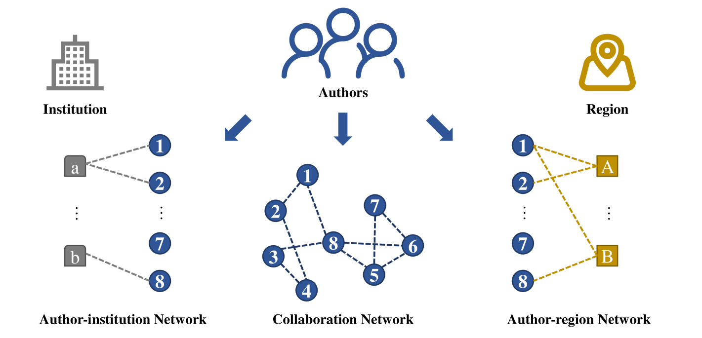
Figure 1: Schematic diagram of the collaboration network, author-institution network, and author-region network. The structural information of author nodes within these bipartite networks can be leveraged to aid in detecting communities within the collaboration network.

To this end, we step outside the framework that relies only on the primary network. We propose an algorithm called Bipartite Assisted Spectral-clustering for Identifying Communities (BASIC) under DCBM and its bipartite modification BiDCBM. We handily integrate the adjacency matrices of both the primary and bipartite networks, then conduct an eigenvalue decomposition toward the aggregated matrix, and apply the SCORE normalization to obtain a new ratio matrix. This crucial step automatically corrects for degree heterogeneity. Finally, we perform clustering on the ratio matrix to obtain the community labels. Using the side information from bipartite networks, the learning performance of the community structures of the primary network can be substantially improved.

The contributions of this paper are threefold. First, to the best of our knowledge, this is the first study to leverage bipartite network information to improve community detection performance. In contrast, existing research focuses primarily on extracting additional insights from the primary network itself, such as nodal covariates or higher-order structures. It is important to note that the proposed BASIC can readily be integrated with existing methods to further tackle weak network signals. It can also be extended to other network models and community detection approaches. Second, we rigorously establish the theoretical guarantee of BASIC by deriving its convergence rate even under extremely weak signals of the primary network. More importantly, we prove that BASIC has a tighter upper bound of the number of error nodes compared to merely using the primary network for community detection, and hence indeed enhances detection power. Third, we collect a large-scale academic network dataset, including collaboration network, author-paper, author-institution, and author-region networks. These datasets serve as valuable resources for investigating community structures in collaborative networks, leading to numerous intriguing and meaningful findings via the proposed BASIC method.

This section ends with some notation. For a vector $\mathbf{v}$ and a fixed integer $q>0$, $\mathbf{v}(i)$ or $v_{i}$ stands for its $i$-th component, $\|\mathbf{v}\|_{q}$ represents its $\ell_{q}$ norm; when $q=2$, we simplify it as $\|\mathbf{v}\|$. When referring to a matrix $\mathbf{M}$, $\mathbf{M}(i,j)$ denotes its $(i,j)$-th entry, $\mathbf{M}_{\bar{i}}$ represents its $i$-th row, $\mathbf{M}_{i\sim j}$ refers to the sub-matrix by removing the $i$-th to $j$-th columns of $\mathbf{M}$. Furthermore, $\|\mathbf{M}\|_{F}$ represents its Frobenius norm, defined as the square root of the sum of the squares of all its elements. Define $\sigma_{\max}(\mathbf{M})$, $\sigma_{\min}(\mathbf{M})$ and $\sigma_{i}(\mathbf{M})$ as the largest, smallest, and $i$-th leading absolute singular value of $\mathbf{M}$, respectively. If $\mathbf{M}$ is a square matrix, denote $\lambda_{\max}(\mathbf{M})$, $\lambda_{\min}(\mathbf{M})$ and $\lambda_{i}(\mathbf{M})$ to be its largest, smallest, and $i$-th leading eigenvalue in absolute values. If further $\mathbf{M}$ is symmetric, $\|\mathbf{M}\|_{op}$ represents its operator norm which equals the largest absolute value of its eigenvalues. For a set $\mathcal{V}$, $|\mathcal{V}|$ denotes its cardinality. When we have two positive sequences $\left\{a_{n}\right\}_{n=1}^{\infty}$ and $\left\{b_{n}\right\}_{n=1}^{\infty}$, use $a_{n}\asymp b_{n}$ to indicate the existence of a constant $C$ such that for large enough $n$, $b_{n}/C\leq a_{n}\leq Cb_{n}$, i.e., $a_{n}$ and $b_{n}$ are of the same order. Denote $a_{n}\gg b_{n}$ if ${a_{n}}/{b_{n}}\to\infty$. Finally, define $\mathbb{I}(A)$ to be the indicator function of event $A$.

2 Methodology of BASIC

2.1 DCBM and BiDCBM for primary and bipartite networks

Denote $\mathcal{G}_{t}=(\mathcal{V}_{t},\mathcal{E}_{t})$ to be the primary network of interest, where $\mathcal{V}_{t}$ and $\mathcal{E}_{t}$ represent the set of primary nodes and edges, respectively. That is, $\mathcal{V}_{t}=\left\{1,\ldots,n\right\}$, with $n$ being the number of primary nodes in $\mathcal{G}_{t}$, and $\mathcal{E}_{t}$ collects the node pairs $(i,j)$ if node $i$ and node $j$ are connected. Define the adjacency matrix of $\mathcal{G}_{t}$ as $\mathbf{A}=\left(\mathbf{A}{(i_{1},i_{2})}\right)\in\mathbb{R}^{n\times n}$, where $i_{1},i_{2}=1,\ldots,n$, that is, $\mathbf{A}{(i_{1},i_{2})}=\mathbb{I}((i_{1},i_{2})\in\mathcal{E}_{t})$. Without loss of generality, set $\mathbf{A}{(i,i)}=0$ for $i=1,\ldots,n$, indicating the absence of self-connections, although the proposed BASIC method can be easily extended to self-connected networks. We utilize the DCBM as the generating model for $\mathcal{G}_{t}$, so that the probability of an edge between two nodes depends only on the communities to which they belong and the degree heterogeneity parameters. Assume that the primary nodes are partitioned into $K$ distinct communities, where $K$ is fixed. For $k=1,\ldots,K$, denote $\mathcal{V}_{t}^{(k)}$, with cardinality $n_{k}=|\mathcal{V}_{t}^{(k)}|$, as the set of node indices in the $k$-th community such that $\mathcal{V}_{t}=\bigcup_{k=1}^{K}\mathcal{V}_{t}^{(k)}$ and $\mathcal{V}_{t}^{(k_{1})}\cap\mathcal{V}_{t}^{(k_{2})}=\emptyset$ for $k_{1}\neq k_{2}$, hence $\sum_{k=1}^{K}n_{k}=n$. Let $\boldsymbol{l}=\left(l_{1},\ldots,l_{n}\right)^{\top}$ be the vector of node membership labels, whose elements take values in $\{1,\ldots,K\}$. The DCBM assumes that the probability of an edge between two nodes is $\mathbf{P}\left(\mathbf{A}{(i_{1},i_{2})}=1\right)={\theta}_{i_{1}}{\theta}_{i_{2}}\mathbf{E}{(l_{i_{1}},l_{i_{2}})}$, where $\mathbf{E}\in\mathbb{R}^{K\times K}$ is a symmetric probability transition matrix between communities with elements in $[0,1]$, and $0\leq{\theta}_{i}\leq 1$ is the degree heterogeneity parameter associated with primary node $i$. A node with a larger ${\theta}_{i}$ value is more likely to connect with other nodes.

In addition, consider $Q$ bipartite networks that are related to the primary network $\mathcal{G}_{t}$, denoted as $\mathcal{G}^{(q)}_{t,s}=(\mathcal{V}_{t},\mathcal{V}^{(q)}_{s},\mathcal{E}^{(q)}_{t,s})$ with $q=1,\ldots,Q$. Specifically, the target nodes set $\mathcal{V}_{t}$ still refers to the set of nodes from the original primary network, while the bipartite nodes set $\mathcal{V}^{(q)}_{s}$ represents the $q$-th set of bipartite nodes. We write $\mathcal{V}_{s}^{(q)}=\left\{1,\ldots,m^{(q)}\right\}$, where $m^{(q)}$ is the number of bipartite nodes in $q$-th bipartite network. Additionally, $\mathcal{E}^{(q)}_{t,s}$ collects the edges in $q$-th bipartite network, which varies among different bipartite networks. For a specific bipartite network $\mathcal{G}_{t,s}^{(q)}$, we can construct a bipartite adjacency matrix $\mathbf{B}^{(q)}=\left(\mathbf{B}^{(q)}{(i,j)}\right)\in\mathbb{R}^{n\times{m^{(q)}}}$, where $\mathbf{B}^{(q)}{(i,j)}=\mathbb{I}((i,j)\in\mathcal{E}^{(q)}_{t,s})$, for $i=1,\ldots,n$ and $j=1,\ldots,m^{(q)}$. We assume that the bipartite nodes can be partitioned into $K^{(q)}$ distinct communities. Let $\boldsymbol{r}^{(q)}=\left(r_{1}^{(q)},\ldots,r_{m}^{(q)}\right)^{\top}$ be the corresponding membership label vector, where $r_{j}^{(q)}$ takes values in $\{1,\ldots,K^{(q)}\}$. To characterize the generative mechanism of bipartite networks, we modify the BiSBM (Yen and Larremore, 2020) by introducing the degree heterogeneity parameters, and the resulting model is named bipartite degree-corrected block model (BiDCBM). Thus, the probability of an edge between two nodes is $\mathbf{P}\left(\mathbf{B}^{(q)}{(i,j)}=1\right)={\theta}_{i}{\delta}^{(q)}_{j}\mathbf{F}^{(q)}{(l_{i},r^{(q)}_{j})}$, where $\mathbf{F}^{(q)}\in\mathbb{R}^{K\times K^{(q)}}$ is an asymmetric probability transition matrix whose elements are in $[0,1]$, and $0\leq{\theta}_{i},{\delta}^{(q)}_{j}\leq 1$ represent the degree heterogeneity parameters associated with primary node $i$ and bipartite node $j$ in $q$-th bipartite network, respectively.

2.2 BASIC: Bipartite Assisted Spectral-clustering for Identifying Communities

Based on the primary network $\mathcal{G}_{t}$ and $Q$ bipartite networks defined in section 2.1, the target is to identify the community structure of primary network, hence, it is important to find an efficient way to aggregate information from the primary and all bipartite networks, even if its signal strength is weak. Solving this problem is not straightforward. For instance, how to tackle the different dimensions among the primary and all bipartite networks? How to extract the community structure information of the bipartite nodes? How to effectively integrate the bipartite information while avoiding the “negative knowledge transfer”? Facing these challenges, we propose a Bipartite Assisted Spectral-clustering method for Identifying Communities, abbreviated as BASIC, by constructing an aggregated square matrix

$$\mathbf{M}=\mathbf{A}\mathbf{A}^{\top}+\sum_{q=1}^{Q}\mathbf{B}^{(q)}\mathbf{B}^{(q)\top}.$$ (1)

The subsequent procedures are applied to this aggregated square matrix $\mathbf{M}\in\mathbb{R}^{n\times n}$ rather than the original scale of adjacency matrices. The formulation of (1) is automatically adapted to different dimensions of individual adjacency matrices from primary and bipartite networks. Moreover, as elaborated in Lemma 2, we prove that this aggregation formulation does not disrupt the community structure of the primary network. This is of utmost importance when integrating side information into the primary objective, which ensures no negative transfer, meaning that the aggregated method performs at least as well as solely using the primary information. Last but not least, this formulation indeed guarantees information enhancement and effectively increases detection power, as shown in Theorem 1. Thus, even if the signal from the primary network, represented by its smallest singular value, is extremely weak, the only requirement for successful community identification is the presence of at least one auxiliary bipartite network with a moderately strong signal. Under these conditions, the convergence rate of community identification is strictly faster than that relying solely on the primary network. All these provide a solid foundation for leveraging diverse data sources to enhance the accuracy and effectiveness of the primary network analyses.

Next, we apply eigenvalue decomposition to $\mathbf{M}$, and extract the first $K$ leading eigenvectors, denoted as $\hat{\mathbf{U}}=\left[\hat{\mathbf{u}}_{1},\hat{\mathbf{u}}_{2},\ldots,\hat{\mathbf{u}}_{K}\right]\in\mathbb{R}^{n\times K}$, which correspond to the community structure of the primary nodes. Subsequently, we apply the SCORE normalization (Jin, 2015) to obtain the ratio matrix $\hat{\mathbf{R}}\in\mathbb{R}^{n\times(K-1)}$, which adjusts to degree heterogeneity by taking the ratio of eigenvectors to the eigenvector corresponding to the largest eigenvalue. Specifically, the elements of the ratio matrix $\hat{\mathbf{R}}$ are defined as

$$\hat{\mathbf{R}}(i,k)=\operatorname{sgn}\left(\hat{\mathbf{u}}_{k+1}(i)\right)\cdot\min\left\{\left|{\hat{\mathbf{u}}_{k+1}(i)}/{\hat{\mathbf{u}}_{1}(i)}\right|,T_{n}\right\},$$ (2)

where $\operatorname{sgn}(x)$ stands for the sign function, i.e., $\operatorname{sgn}(x)=1$ when $x>0$, $\operatorname{sgn}(0)=0$, and $\operatorname{sgn}(x)=-1$ when $x<0$. In addition, $T_{n}$ is a threshold, generally set to $\log(n)$. Last, we conduct the $k$-means algorithm on the rows of the ratio matrix $\hat{\mathbf{R}}$ and obtain the detected communities. Algorithm 1 summarizes the step-by-step procedure of BASIC.

Algorithm 1 The procedure of BASIC for community detection

1. The adjacency matrix of the primary network $\mathbf{A}$, the number of communities $K$ for the primary nodes, the adjacency matrices of bipartite networks $\mathbf{B}^{(q)}$ for $q=1,\ldots,Q$.

2. Compute the aggregated matrix $\mathbf{M}$ by (1).

3. Apply the eigenvalue decomposition to $\mathbf{M}$ and obtain the first $K$ leading eigenvectors $\hat{\mathbf{U}}=\left[\hat{\mathbf{u}}_{1},\hat{\mathbf{u}}_{2},\ldots,\hat{\mathbf{u}}_{K}\right]\in\mathbb{R}^{n\times K}$.

4. Compute the ratio matrix $\hat{\mathbf{R}}\in\mathbb{R}^{n\times(K-1)}$ in (2).

5. Apply the $k$-means algorithm to the columns of $\hat{\mathbf{R}}$, and solve for

   $$\mathbf{N}^{*}=\underset{\mathbf{N}\in\mathcal{N}_{n,K-1,K}}{\operatorname{argmin}}\|\mathbf{N}-\hat{\mathbf{R}}\|_{F}^{2},$$

   where $\mathcal{N}_{n,K-1,K}$ represents the set of $n\times(K-1)$ matrices with only $K$ distinct rows.

6. Utilize $\mathbf{N}^{*}$ to assign the membership of primary nodes, $\hat{\boldsymbol{l}}=(\hat{l}_{1},\ldots,\hat{l}_{n})^{\top}$.

7. Community label vector $\hat{\boldsymbol{l}}=(\hat{l}_{1},\ldots,\hat{l}_{n})^{\top}$.

3 Theoretical Guarantee of BASIC

3.1 Rationale of BASIC on Population Level

To establish the theoretical foundation of BASIC, we first analyze the population counterpart of the aggregated square matrix $\mathbf{M}$ proposed in (1). Specifically, denote by $\boldsymbol{\Omega}^{(0)}=\mathbb{E}[\mathbf{A}]\in\mathbb{R}^{n\times n}$ the expectation of the adjacency matrix $\mathbf{A}$ and $\boldsymbol{\Omega}^{(q)}=\mathbb{E}[\mathbf{B}^{(q)}]\in\mathbb{R}^{n\times m^{(q)}}$ the expectation of adjacency matrix $\mathbf{B}^{(q)}$ for $q=1,\ldots,Q$. Then define the population aggregated square matrix $\boldsymbol{\Omega}_{M}$ as

$$\boldsymbol{\Omega}_{M}=\boldsymbol{\Omega}^{(0)}\boldsymbol{\Omega}^{(0)\top}+\sum_{q=1}^{Q}\boldsymbol{\Omega}^{(q)}\boldsymbol{\Omega}^{(q)\top}.$$ (3)

Then, $\boldsymbol{\Omega}_{M}$ can serve as the population counterpart of $\mathbf{M}$.

Next, we discuss the rationality of BASIC, by aligning the eigenvectors of $\boldsymbol{\Omega}_{M}$ with the original inherent community structure. Given that bipartite nodes are not the focus of this work, for the sake of notation simplicity, we assume that all bipartite networks share the same number of communities for bipartite nodes, the same node size, and the same degree heterogeneity parameters. That is, for $q=1,\ldots,Q$, assume $K^{(q)}\equiv K^{\prime}$, $m^{(q)}\equiv m$, and $\delta_{j}^{(q)}\equiv\delta_{j}$. Define the degree heterogeneity vectors for primary and bipartite nodes as $\boldsymbol{\theta}=(\theta_{1},\ldots,\theta_{n})^{\top}\in\mathbb{R}^{n}$ and $\boldsymbol{\delta}=(\delta_{1},\ldots,\delta_{m})^{\top}\in\mathbb{R}^{m}$, respectively. Let $\theta_{\min}\equiv\min_{1\leqslant i\leqslant n}\theta_{i}$, $\theta_{\max}\equiv\max_{1\leqslant i\leqslant n}\theta_{i}$, $\delta_{\min}\equiv\min_{1\leqslant i\leqslant m}\delta_{i}$, and $\delta_{\max}\equiv\max_{1\leqslant i\leqslant m}\delta_{i}$. In addition, define community-specific degree heterogeneity vectors as $\boldsymbol{\theta}^{(k)}\in\mathbb{R}^{n}$ and $\boldsymbol{\delta}^{(k^{\prime})}\in\mathbb{R}^{m}$ for $k=1,\ldots,K$ and $k^{\prime}=1,\ldots,K^{\prime}$, where $\theta^{(k)}_{i}=\theta_{i}\mathbb{I}(l_{i}=k)$ and $\delta^{(k^{\prime})}_{i}=\delta_{i}\mathbb{I}(r_{i}=k^{\prime})$, with the membership labels $l_{i}$ and $r_{i}$ defined in Section 2.1. Furthermore, define the orthonormal membership matrices, $\boldsymbol{\Theta}_{\boldsymbol{\theta}}\in\mathbb{R}^{n\times K}$ and $\boldsymbol{\Theta}_{\boldsymbol{\delta}}\in\mathbb{R}^{n\times K^{\prime}}$, as $\boldsymbol{\Theta}_{{\theta}}(i,k)={{\theta}_{i}}/{\|\boldsymbol{\theta}^{(k)}\|}\mathbb{I}(l_{i}=k)$ and $\boldsymbol{\Theta}_{\boldsymbol{\delta}}(i,k^{\prime})={{\delta}_{i}}/{\|\boldsymbol{\delta}^{(k^{\prime})}\|}\mathbb{I}(r_{i}=k^{\prime})$, for $i=1,\ldots,n$, $k=1,\ldots,K$, and $k^{\prime}=1,\ldots,K^{\prime}$. Then the community memberships of primary nodes can be directly reflected by matrix $\boldsymbol{\Theta}_{\boldsymbol{\theta}}$, since by its definition, node $i$ belongs to community $k$ if $\boldsymbol{\Theta}_{\boldsymbol{\theta}}(i,k)\neq 0$. Define two diagonal matrices $\boldsymbol{\Psi}_{\boldsymbol{\theta}}\in\mathbb{R}^{K\times K}$ and $\boldsymbol{\Psi}_{\boldsymbol{\delta}}\in\mathbb{R}^{K^{\prime}\times K^{\prime}}$ with $\boldsymbol{\Psi}_{\boldsymbol{\theta}}(k,k)={\|\boldsymbol{\theta}^{(k)}\|}/{\|\boldsymbol{\theta}\|}$ and $\boldsymbol{\Psi}_{\boldsymbol{\delta}}(k^{\prime},k^{\prime})={\|\boldsymbol{\delta}^{(k^{\prime})}\|}/{\|\boldsymbol{\delta}\|}$. The diagonal elements in $\boldsymbol{\Psi}_{\boldsymbol{\theta}}$ and $\boldsymbol{\Psi}_{\boldsymbol{\delta}}$ are indeed the community heterogeneity parameters corresponding to the primary and bipartite nodes, respectively. Simple calculation yields

$$\boldsymbol{\Omega}^{(0)}=\|\boldsymbol{\theta}\|^{2}\boldsymbol{\Theta}_{\theta}\mathbf{S}^{(0)}\boldsymbol{\Theta}_{\theta}^{\top}\quad\text{ and }\quad\boldsymbol{\Omega}^{(q)}=\|\boldsymbol{\theta}\|\|\boldsymbol{\delta}\|\boldsymbol{\Theta}_{\theta}\mathbf{S}^{(q)}\boldsymbol{\Theta}_{\delta}^{\top},\ \ q=1,\ldots,Q,$$

where $\mathbf{S}^{(0)}=\boldsymbol{\Psi}_{\boldsymbol{\theta}}\mathbf{E}\boldsymbol{\Psi}_{\boldsymbol{\theta}}^{\top}\in\mathbb{R}^{K\times K}$ and $\mathbf{S}^{(q)}=\boldsymbol{\Psi}_{\boldsymbol{\theta}}\mathbf{F}^{(q)}\boldsymbol{\Psi}_{\boldsymbol{\delta}}^{\top}\in\mathbb{R}^{K\times K^{\prime}}$ can be viewed as the probability transition matrices with community heterogeneity. Then, $\boldsymbol{\Omega}_{M}$ can be reparameterized as

$$\boldsymbol{\Omega}_{M}=\left\|\boldsymbol{\theta}\right\|^{2}\left\|\boldsymbol{\delta}\right\|^{2}\boldsymbol{\Theta}_{\theta}\bar{\mathbf{S}}\boldsymbol{\Theta}_{\theta}^{\top},$$ (4)

where $\bar{\mathbf{S}}\equiv\left(\left\|\boldsymbol{\theta}\right\|^{2}/\left\|\boldsymbol{\delta}\right\|^{2}\right)\mathbf{S}^{(0)}\mathbf{S}^{(0)\top}+\sum_{q=1}^{Q}\left(\mathbf{S}^{(q)}\mathbf{S}^{(q)\top}\right)$.

Based on the representation of $\boldsymbol{\Omega}_{M}$ in (4), Proposition 1 below shows that the eigen-structure of $\boldsymbol{\Omega}_{M}$ parallels the community structure of primary nodes.

Proposition 1

Let $\boldsymbol{\Omega}_{M}=\mathbf{U}\boldsymbol{\Lambda}\mathbf{U}^{\top}$ be the compact eigenvalue decomposition of $\boldsymbol{\Omega}_{M}$, then the $i$-th leading eigenvalue of $\boldsymbol{\Omega}_{M}$ is

$$\lambda_{i}(\boldsymbol{\Omega}_{M})=\begin{cases}\left\|\boldsymbol{\theta}\right\|^{2}\left\|\boldsymbol{\delta}\right\|^{2}\lambda_{i}(\bar{\mathbf{S}})&\text{ if }\quad 1\leqslant i\leqslant K,\\ 0&\text{ if }\quad i>K.\end{cases}$$ (5)

Further let $\bar{\mathbf{S}}=\mathbf{J}\boldsymbol{\Sigma}\mathbf{J}^{\top}$ be the eigenvalue decompositions of $\bar{\mathbf{S}}$. Then the $i$-th row of eigenvectors of $\boldsymbol{\Omega}_{M}$ can be expressed as

$$\mathbf{U}_{\bar{i}}=\frac{{\theta}_{i}}{\|\boldsymbol{\theta}^{\left(l_{i}\right)}\|}\mathbf{J}_{\bar{l_{i}}}\quad\text{for}\quad 1\leqslant i\leqslant n,$$ (6)

and $\left\|\mathbf{U}_{\bar{i}}\right\|\asymp{{\theta}_{i}}/{\|\boldsymbol{\theta}\|}$.

Proposition 1 implies that the rank of original aggregated matrix $\boldsymbol{\Omega}_{M}\in\mathbb{R}^{n\times n}$ is at most $K$, and connects this $n\times n$ matrix with a low-dimensional matrix $\bar{\mathbf{S}}\in\mathbb{R}^{K\times K}$. It also explains the rationale of applying the SCORE-type normalization (2) to $\boldsymbol{\Omega}_{M}$ upon spectral clustering. Take two primary nodes $i_{1}$ and $i_{2}$ for instance, with $\mathbf{U}_{\bar{i_{1}}}=({{\theta}_{i_{1}}}/{\|\boldsymbol{\theta}^{(l_{i_{1}})}\|})\mathbf{J}_{\bar{l_{i_{1}}}}$ and $\mathbf{U}_{\bar{i_{2}}}=({{\theta}_{i_{2}}}/{\|\boldsymbol{\theta}^{(l_{i_{2}})}\|})\mathbf{J}_{\bar{l_{i_{2}}}}$. If nodes $i_{1}$ and $i_{2}$ belong to the same community, the only difference between $\mathbf{U}_{\bar{i_{1}}}$ and $\mathbf{U}_{\bar{i_{2}}}$ lies in their degree heterogeneity parameters ${\theta}_{i_{1}}$ and ${\theta}_{i_{2}}$, which can be eliminated by SCORE-normalization. Thus, clustering rows of $\mathbf{U}$ after SCORE-normalization automatically recovers the original community structure.

3.2 Theoretical Guarantee of BASIC

To explore the theoretical privilege of BASIC based on the observed aggregated square matrix $\mathbf{M}$, we first impose several assumptions on the probability transition matrices and heterogeneity parameters. Recall $\mathbf{E}$ and $\mathbf{F}^{(q)}$ represent the $K\times K$ and $K\times K^{(q)}$ low-dimensional probability transition matrices among communities for the primary and the $q$-th bipartite network, respectively.

Assumption 1

The matrices $\mathbf{E}\mathbf{E}^{\top}$ and $\mathbf{F}^{(q)}\mathbf{F}^{(q)\top}$ with $1\leqslant q\leqslant Q$ are irreducible.

Assumption 2

There exists at least one probability transit matrix among the primary and bipartite networks, such that the largest singular value (or eigenvalue for primary network) is of higher order than $\sqrt{\log(n)Z}/(\|\boldsymbol{\theta}\|\|\boldsymbol{\delta}\|)$, where $Z\equiv\max\left(\theta_{\max},\delta_{\max}\right)\max\left(\|\boldsymbol{\theta}\|_{1},\|\boldsymbol{\delta}\|_{1}\right)$.

Assumption 3

The degree heterogeneity parameters satisfy that $\|\boldsymbol{\theta}\|\asymp\|\boldsymbol{\delta}\|$, $\|\boldsymbol{\theta}^{(k)}\|\asymp\|\boldsymbol{\theta}^{(l)}\|$, and $\|\boldsymbol{\delta}^{(k^{\prime})}\|\asymp\|\boldsymbol{\delta}^{(l^{\prime})}\|$ for $k,l=1,\ldots,K$ and $k^{\prime},l^{\prime}=1,\ldots,K^{\prime}$. In addition, $\lim_{n\rightarrow\infty}{\log(n)Z}/{{\theta}_{\min}{\delta}_{\min}\|\boldsymbol{\theta}\|_{1}\|\boldsymbol{\delta}\|_{1}}=0$.

The irreducibility condition in Assumption 1, commonly used in network analysis, implies that no permutation of rows or columns can transform the matrix into a block diagonal form. According to Perron-Frobenius Theorem (Perron, 1907; Frobenius, 1912), Assumption 1 ensures that all entries in the leading eigenvector of the aggregated matrix $\boldsymbol{\Omega}_{\mathbf{M}}$ are strictly positive, and hence the ratio matrix in (2) is well-defined. Assumption 2 requires at least one network possesses spike structure, meaning that the corresponding largest eigenvalue is far larger than that of the error matrix; see the detailed discussion in (12). Assumption 3 requires the degree heterogeneity parameters between the primary and the bipartite networks, as well as among all communities within each network, to possess the same order. This implies that the community sizes are not be extremely imbalanced, and no community size approaches zero. Similar conditions can be found in consistent community detection methods, such as Jin (2015); Wang et al. (2020).

Based on the imposed assumptions, we first derive an upper bound of the distance between the observed aggregated matrix $\mathbf{M}$ and its population counterpart $\boldsymbol{\Omega}_{M}$ in Lemma 1.

Lemma 1

Under Assumptions 1, 2 and 3, with probability at least $1-o\left(n^{-4}\right)$, we have

$$\left\|\mathbf{M}-\boldsymbol{\Omega}_{\mathbf{M}}\right\|_{op}\lesssim\left\|\boldsymbol{\theta}\right\|\left\|\boldsymbol{\delta}\right\|\sqrt{\log(n)Z}\max\left\{\max_{q=1}^{Q}\sigma_{\max}\left(\mathbf{F}^{(q)}\right),\lambda_{\max}(\mathbf{E})\right\}.$$

Lemma 1 studies the estimation error for substituting the population aggregated matrix $\boldsymbol{\Omega}_{M}$ with its observed counterpart $\mathbf{M}$. Under mild conditions to be discussed below Theorem 1, this bound is dominated by the maximum eigenvalue of $\boldsymbol{\Omega}_{M}$ on the asymptotic sense, which further ensures a vanishing mis-clustering rate of BASIC in Theorem 1.

To study the mis-clustering rate of BASIC, we follow Wang et al. (2020) and define $\mathcal{W}=\{1\leqslant i\leqslant$ $\left.n:\left\|\mathbf{N}_{\bar{i}}^{*}-\mathbf{R}_{\bar{i}}\right\|\leqslant{1}/{2}\right\}$ as the set of nodes that are accurately clustered by BASIC, and thus $\mathcal{V}_{t}\backslash\mathcal{W}$ consists of nodes that are mis-clustered. Theorem 1 establishes a non-asymptotic bound for the mis-clustering rate of BASIC.

Theorem 1

Under Assumptions 1, 2 and 3, with probability at least $1-o\left(n^{-4}\right)$, the mis-clustering rate of BASIC satisfies

$$\frac{|\mathcal{V}_{t}\backslash\mathcal{W}|}{n}\lesssim\frac{\log(n)ZT_{n}^{2}}{n\theta_{\min}^{2}\left\|\boldsymbol{\theta}\right\|^{4}}\left(\operatorname{SNR}^{\operatorname{BASIC}}\right)^{-2},$$

where $T_{n}=\log(n)$, and

$$\operatorname{SNR}^{\operatorname{BASIC}}=\frac{\sum_{q=1}^{Q}\sigma^{2}_{\min}\left(\mathbf{F}^{(q)}\right)+\lambda^{2}_{\min}\left(\mathbf{E}\right)}{\max\left\{\max_{q=1}^{Q}\sigma_{\max}\left(\mathbf{F}^{(q)}\right),\lambda_{\max}(\mathbf{E})\right\}}.$$

The proof of Theorem 1 is given in Appendix B.3. In Theorem 1, $\operatorname{SNR}^{\operatorname{BASIC}}$ can be understood as the integrated signal-to-noise ratio (SNR) of all networks involved. If $\operatorname{SNR}^{\operatorname{BASIC}}\gg\sqrt{{\log(n)ZT_{n}^{2}}/{n\theta_{\min}^{2}\left\|\boldsymbol{\theta}\right\|^{4}}}$, the mis-clustering rate $|\mathcal{V}_{t}\backslash\mathcal{W}|/n\to 0$ as $n\to\infty$. To demonstrate the merit of BASIC through Theorem 1, for a fair comparison, we also derive the mis-clustering rate for the primary network alone under the same theoretical framework, which is

$$\frac{|\mathcal{V}_{t}\backslash\mathcal{W}|}{n}\lesssim\frac{\log(n)ZT_{n}^{2}}{n\theta_{\min}^{2}\left\|\boldsymbol{\theta}\right\|^{4}}\left(\frac{\lambda_{\max}\left(\mathbf{E}\right)}{\lambda^{2}_{\min}\left(\mathbf{E}\right)}\right)^{2}\equiv\frac{\log(n)ZT_{n}^{2}}{n\theta_{\min}^{2}\left\|\boldsymbol{\theta}\right\|^{4}}(\operatorname{SNR}^{\operatorname{Primary}})^{-2},$$ (7)

where $\operatorname{SNR}^{\operatorname{Primary}}=\lambda^{2}_{\min}(\mathbf{E})/\lambda_{\max}(\mathbf{E})$ is the corresponding signal-to-noise ratio of primary network solely. A similar definition of SNR has been used in Jin et al. (2021, 2023). The above non-asymptotic bound in (7) highly relies on the minimal signal $\lambda_{\min}\left(\mathbf{E}\right)$ of the primary network, thus it easily diverges for weak-signal primary networks where $\lambda_{\min}\left(\mathbf{E}\right)$ goes to zero. On the other hand, according to Theorem 1, BASIC leverages the risk of divergence by introducing the bipartite information, then the mis-clustering rate can still vanish if only one of bipartite networks is not of weak-signal. In practice, $\operatorname{SNR}^{\operatorname{BASIC}}$ typically enhances $\operatorname{SNR}^{\operatorname{Primary}}$, leading to faster convergence of the mis-clustering rate, since the numerator of the former consists of the summation of minimal signals from all involved networks, while its enlarged denominator only takes one of the maximum signals. Especially, if $\sigma_{\max}\left(\mathbf{F}^{(q)}\right)\asymp\lambda_{\max}(\mathbf{E})$ for $q=1,\ldots,Q$, indicating all bipartite networks have spike structure, then the asymptotic relative gain from BASIC is

$$\frac{\operatorname{SNR}^{\operatorname{BASIC}}}{\operatorname{SNR}^{\operatorname{Primary}}}\asymp\frac{\sum_{q=1}^{Q}\sigma^{2}_{\min}\left(\mathbf{F}^{(q)}\right)+\lambda^{2}_{\min}\left(\mathbf{E}\right)}{\lambda^{2}_{\min}(\mathbf{E})}.$$

That is, the learning performance of the community structures of the primary network can be substantially enhance, only if at least one of bipartite networks has non-degenerating signal $\sigma^{2}_{\min}\left(\mathbf{F}^{(q)}\right)$.

Furthermore, even if all bipartite networks are in fact pure noise, with $\sigma_{\min}(\mathbf{F}^{(q)})\ll\sqrt{\log(n)Z}/(\|\boldsymbol{\theta}\|\|\boldsymbol{\delta}\|)$, $q=1,\ldots,Q$, but the primary network contains relatively strong signals. We can obtain $\max\left\{\max_{q=1}^{Q}\sigma_{\max}\left(\mathbf{F}^{(q)}\right),\lambda_{\max}(\mathbf{E})\right\}=\lambda_{\max}(\mathbf{E})$ and $\sum_{q=1}^{Q}\sigma^{2}_{\min}\left(\mathbf{F}^{(q)}\right)+\lambda^{2}_{\min}\left(\mathbf{E}\right)\asymp\lambda^{2}_{\min}\left(\mathbf{E}\right)$. Hence, we have

$$\operatorname{SNR}^{\operatorname{BASIC}}\asymp\frac{\lambda^{2}_{\min}\left(\mathbf{E}\right)}{\lambda_{\max}(\mathbf{E})},$$

which matches $\operatorname{SNR}^{\operatorname{Primary}}$. This indicates that BASIC naturally prevents negative knowledge transfer when incorporating bipartite information.

4 Simulation

In this section, we assess the performance of the proposed BASIC method under the DCBM for the primary network and the BiDCBM for bipartite networks, under both weak and strong signal conditions of the primary network. We investigate how bipartite networks with varying signal strengths can indeed enhance community detection, and verify that the clustering performance is not degraded even if the added bipartite information is weak. We consider various combinations of node sizes and the number of communities, addressing both balanced and imbalanced community structures. To evaluate the clustering accuracy of BASIC, we calculate the Adjusted Rand Index (ARI) (Hubert and Arabie, 1985) that reflects the consistency between the clustering results and the inherent true labels, ranging from -1 to 1. A higher ARI value indicates higher clustering accuracy. The SCORE method (Jin, 2015) applied to the primary network is treated as baseline.

4.1 Simulation Setup

We generate the mean matrices $\Omega^{(0)}$ and $\Omega^{(q)}$, $q=1,\ldots,Q$, for the primary and bipartite networks, respectively, following Li et al. (2020). We take three combinations of $\{n,m,K\}$: $\{600,300,3\}$, $\{600,300,5\}$, and $\{1200,600,5\}$. For the community structure of our primary interest, both balanced and imbalanced community sizes are considered. In balanced cases, all communities have the same sizes $n/K$. In imbalanced cases, the community sizes of the primary nodes are respectively set to $\{100,200,300\}$, $\{50,100,100,150,200\}$ and $\{100,200,200,300,400\}$. Then assign the node membership labels $\boldsymbol{l}=(l_{1},\ldots,l_{n})^{\top}$ and $\boldsymbol{r}^{(q)}=(r_{1}^{(q)},\ldots,r_{m}^{(q)})^{\top}$, without loss of generality, in a sequential manner. Taking the balanced case for instance,

$$\boldsymbol{l}=(\underbrace{1,\ldots,1}_{n/K},\underbrace{2,\ldots,2}_{n/K},\ldots,\underbrace{K,\ldots,K}_{n/K})^{\top}.$$

Given $\boldsymbol{l}$, further define the community membership matrix $\mathbf{X}\in\mathbb{R}^{n\times K}$ for the primary network, where $\mathbf{X}(i,k)=\mathbb{I}$($l_{i}=k$) for $i=1,\ldots,n$ and $k=1,\dots,K$. In addition, take $\boldsymbol{\Pi}=(1-\beta)\mathbf{I}_{K}+\beta\mathbf{1}_{K}\mathbf{1}_{K}^{\top}$, where $\mathbf{I}_{K}$ is a $K\times K$ identity matrix and $\mathbf{1}_{K}$ denotes a column vector of length $K$ with every entry being 1, and $\beta$ represents the common out-in ratio, i.e., the ratio of between-block and within-block probability of edges. The values of $\beta$ will be specified later in different scenarios. As $\beta$ increases, the communities become less distinguishable, resulting in weak-signal networks. Last, we draw a vector of node degree parameter $\mathbf{d}=(d_{1},\ldots,d_{n})^{\top}$ from a power-law distribution with lower bound 1 and scaling parameter 5. When normalized to the range between 0 and 1, $\mathbf{d}$ corresponds to the vector of degree heterogeneity parameter $\boldsymbol{\theta}$ in Section 3.1. Given all the above quantities, we can define the mean matrix $\boldsymbol{\Omega}^{(0)}\propto\mbox{diag}(\mathbf{d})\mathbf{X}\boldsymbol{\Pi}\mathbf{X}^{\top}\mbox{diag}(\mathbf{d})^{\top}$ according to the DCBM, so that the probability of an edge between nodes only depends on the community structure $\mathbf{X}$ and the node degree parameter $\mathbf{d}$. We can specify a normalizing factor when generating $\boldsymbol{\Omega}^{(0)}$ to adjust the average node degree in the network, aiming to prevent the network from being too dense or sparse. In our simulation, we set the average degree to be 40. In the same fashion, we can generate the mean matrices $\boldsymbol{\Omega}^{(q)}$, $q=1,\ldots,Q$ for the bipartite networks. Here we take $Q=5$. All simulation results are based on 200 replications.

4.2 Simulation Results

We evaluate the performance of BASIC under various signal conditions of primary and bipartite networks. Firstly, we consider the weak-signal primary network, with the out-in ratio $\beta$ of the primary network set to $0.5$ (Li et al., 2020). Recall that a larger $\beta$ leads to a weaker signal. Then, we vary the out-in ratios of the 5 bipartite networks in the following four cases:

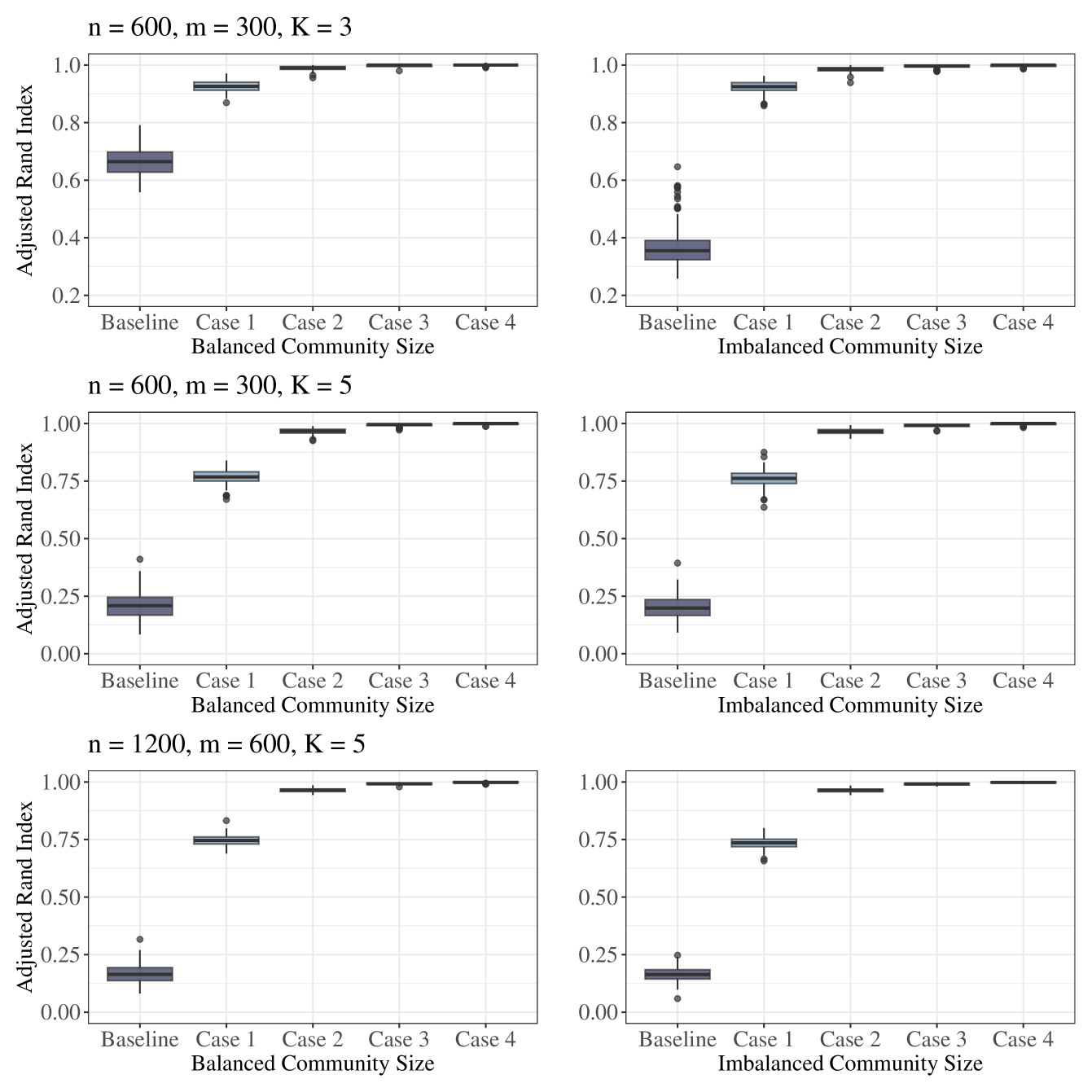
Figure 2: ARI for weak-signal primary networks. The baseline refers to the results obtained by using only the primary network. Cases 1, 2, 3, and 4 correspond to using 0, 1, 2, and 3 strong bipartite networks, respectively.

• Case 1: $0.5,0.5,0.5,0.5,0.5$ (5 weak signals)

• Case 2: $0.1,0.5,0.5,0.5,0.5$ (1 strong and 4 weak signals)

• Case 3: $0.1,0.1,0.5,0.5,0.5$ (2 strong and 3 weak signals)

• Case 4: $0.1,0.1,0.1,0.5,0.5$ (3 strong and 2 weak signals)

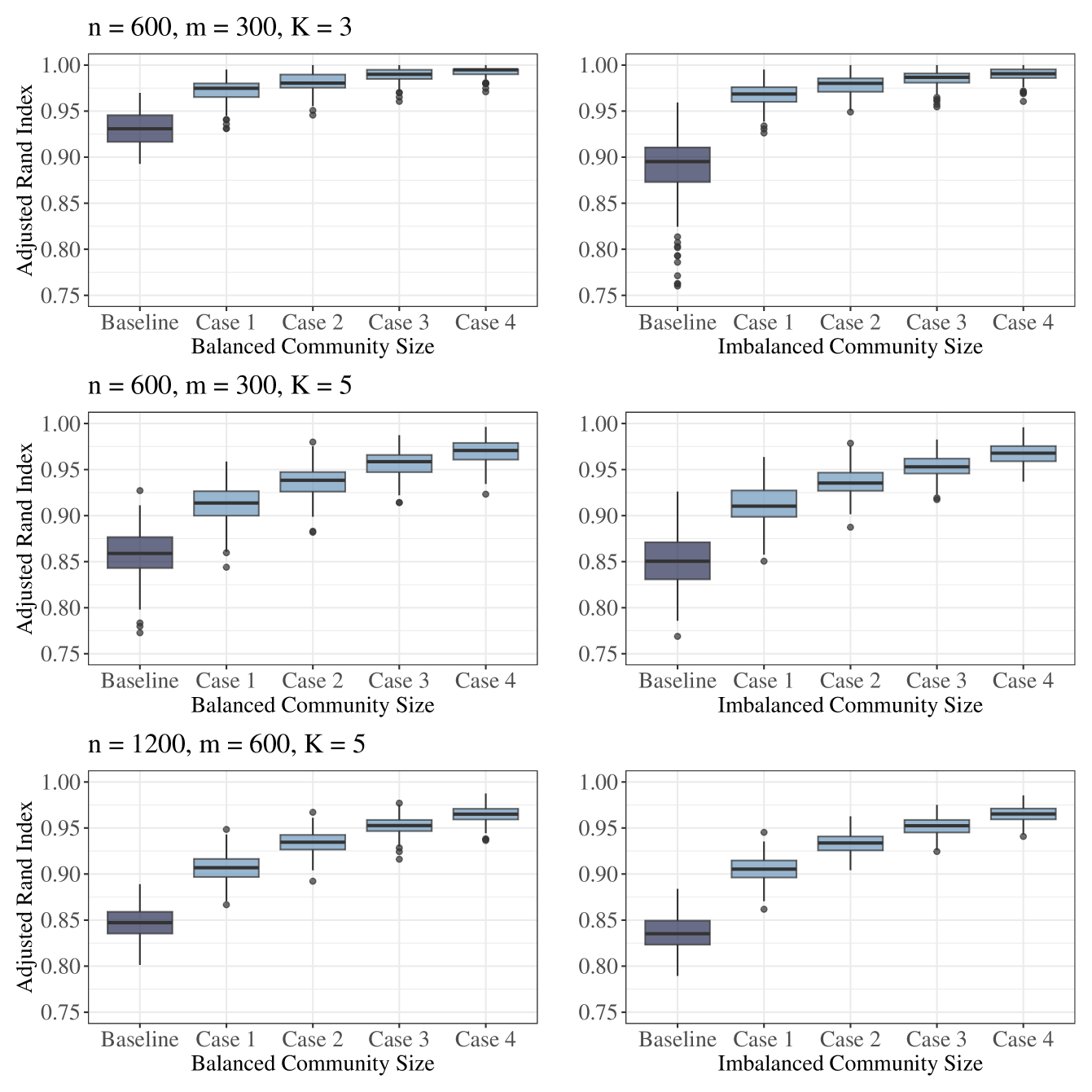
Figure 3: ARI for strong-signal primary networks. The baseline refers to the results obtained by using only the primary network. Cases 1, 2, 3, and 4 correspond to using 0, 1, 2, and 3 bipartite networks with the same signal strength as the primary network, respectively.

The above four cases correspond to the use of 0, 1, 2, and 3 strong bipartite networks, respectively. The results of community detection are illustrated in Figure 2, where the baseline SCORE method uses only the primary network. We observe obvious enhancement of ARI by incorporating bipartite information, for both balanced and imbalanced community sizes. The ARI of the baseline is around 0.25 in all four cases. This is consistent with our theoretical result (7) - for weak-signal primary networks, the mis-clustering rate easily diverges. Furthermore, the performance of BASIC is further improved as more strong-signal bipartite networks are incorporated. Last but not least, we observe that even if all five bipartite networks are weak-signal ones (Case 1), the enhancement is still obvious.

Secondly, we set the community structure signal of the primary network to be relatively strong, with the out-in ratio $\beta$ of the primary network being $0.3$. We aim to investigate whether incorporating the bipartite network can further enhance performance or, at the very least, prevent degradation. We set 0, 1, 2, and 3 bipartite networks with out-in ratios equal to that of the primary network, while the other bipartite networks set to $0.5$.

• Case 1: $0.5,0.5,0.5,0.5,0.5$ (5 weak signals)

• Case 2: $0.3,0.5,0.5,0.5,0.5$ (1 strong and 4 weak signals)

• Case 3: $0.3,0.3,0.5,0.5,0.5$ (2 strong and 3 weak signals)

• Case 4: $0.3,0.3,0.3,0.5,0.5$ (3 strong and 2 weak signals)

The results are depicted in Figure 3. The performances of the baseline in most cases are already fairly satisfactory due to the relatively strong signal from the primary network. However, leveraging information from bipartite networks can further enhance the performance of community detection in the primary network. Additionally, as shown in Case 1, even when the community structure of the bipartite networks is unclear, utilizing BASIC does not deteriorate the community detection. These phenomena are observed in both balanced and imbalanced cases and are consistent with the theoretical results in Theorem 1.

5 Real Data Analysis: Structure Learning of Author Collaboration Network

5.1 Data Description

Table 1: An illustrative example of a statistical publication. Basic information such as title, abstract, keywords, citation counts, author information, and reference list are obtained. The citation counts are provided by the Web of Science up to 2022.

Variable	Example
Title	A proportional hazards model for the subdistribution of a competing risk
Abstract	With explanatory covariates, the standard analysis for competing risks data involves modeling the cause-specific hazard functions via a proportional hazards assumption…
Keywords	hazard of subdistribution; martingale; partial likelihood; transformation model
Journal	JASA
Year	1999
Citation counts	8,265 (until 2022)
Author information	Fine, Jason P.@ University of Pittsburgh; Gray, Robert J.@Harvard University
Reference list	$\left[1\right]$ Nonparametric estimation of partial transition-probabilities in multiple decrement models@Aalen, O@1978@AoS $\left[2\right]$ Estimates of absolute cause-specific risk in cohort studies Benichou, J & Gail, MH@1990@Biometrics $\left[3\right]$ …

In this section, we utilize the proposed BASIC method to analyze an author collaboration network dataset. We collect statistical publications from 42 renowned statistical journals from 1981 to 2021 in Web of Science (www.webofscience.com). We obtain titles, abstracts, keywords, citation counts up to 2022, years, journals, author information (including names, institutions, and regions) and reference lists, as illustrated in Table 1. After a challenging data cleaning process, we construct a collaboration network with 16,125 nodes and 22,530 edges as the original network: the nodes represent the authors, with an undirected and unweighted edge between two authors if they have published two or more papers together (Zhang et al., 2023; Ji et al., 2022). The resulting collaboration network has a density of 0.017%, indicating that it is very sparse. To concentrate on the most important nodes, we extract the $c$-core network by iteratively removing nodes with a degree less than $c$ until the network stabilizes (Wang and Rohe, 2016). The $c$-core network is a commonly used method for extracting core information from networks (Miao and Li, 2023; Ding et al., 2023). Specifically, we extract the 4-core of the collaboration network and obtain the largest connected component, resulting in a core network with 737 nodes and 2,453 edges, with a network density of 0.904%. This core network serves as the primary network for community detection. In addition, author information can help us obtain the corresponding institution and region of the authors. Therefore, we consider three bipartite networks: the author-paper network, the author-institution network, and the author-region network.

5.2 Community Detection by BASIC

In this subsection, we use information from three bipartite networks, from the perspectives of papers, institutions, and regions, to assist the community structure learning of the primary collaboration network. The SCORE method applied to the collaboration network is treated as the baseline. The number of communities $K$ in the primary network is determined by the edge cross-validation (ECV) algorithm (Li et al., 2020). Specifically, we set the maximum number of communities to 30 according to the scree plot as illustrated in Figure 8. By repeating the ECV process 20 times for $K$ from 1 to 30, we obtain the optimal number of communities as 12. According to Jin et al. (2021), the eigenvalues of a weak-signal network often have the $K$-th and $(K+1)$-th values that are “close”. When $K=12$, we compute the quantity $1-{\hat{\lambda}_{K+1}}/{\hat{\lambda}_{K}}=0.011$, which is smaller than the commonly used scale-free threshold of 0.1. This result highlights that the collaboration network is indeed a weak-signal network. In contrast, for typical strong signal networks, this quantity exceeds 0.1, such as in the Karate (0.414) (Zachary, 1977) and Polblogs (0.6) (Adamic and Glance, 2005) networks.

Table 2: Utilizing the information from three bipartite networks: author-paper, author-institution, and author-region networks to assist the community detection results of the primary network (collaboration network). Communities are sorted by size in descending order.

ID	Size	Author	Keywords
1	148	Balakrishnan, Narayanaswamy	Order statistics, Maximum likelihood
		Hothorn, Torsten	EM algorithm, Exponential distribution
		Rao, J. N. K.	Weibull distribution, Monte Carlo simulation
		Kundu, Debasis	Birnbaum-Saunders distribution, Likelihood ratio test
		Cordeiro, Gauss Moutinho	Censored data, Local influence
2	139	Tibshirani, Robert	Survival analysis, Bootstrap
		Hastie, Trevor J.	Causal inference, LASSO
		Friedman, Jerome H.	Functional data analysis, Nonparametric regression
		Fine, Jason P.	EM algorithm, Variable selection
		Wei, Lee-Jen	Missing data, Robustness
3	91	Bai, Zhidong	Asymptotic normality, Variable selection
		Li, Wai-Keung	Longitudinal data, Empirical likelihood
		Fang, Kaitai	Quantile regression, Oracle property
		Peng, Heng	Robustness, EM algorithm
		Yin, Guosheng	Estimating equations, High-dimensional data
4	75	Carlin, Bradley P.	Markov chain Monte Carlo, Gibbs sampling
		Gelfand, Alan. E.	Bayesian inference, Dirichlet process
		Cook, R. Dennis	Gaussian process, Empirical Bayes
		Casella, George	Variable selection, Central subspace
		Wu, C. F. Jeff	Minimaxity, Hierarchical model
5	57	Fan, Jianqing	Variable selection, LASSO
		Li, Runze	EM algorithm, Model selection
		Zou, Hui	Empirical likelihood, Asymptotic normality
		Tsai, Chih-Ling	Oracle property, Estimating equation
		Hornik, Kurt	High-dimensional data, SCAD
6	45	Hall, Peter Gavin	Bootstrap, Robustness
		Zeileis, Achim	Bandwidth, Kernel methods
		Mukerjee, Rahul	Consistency, Small area estimation
		Cuevas, Antonio	Nonparametric regression, Mean squared error
		Basu, Analabha	Density estimation, Influence function
7	40	Rousseeuw, Peter J.	Linear mixed model, Missing data
		Kenward, Michael G.	Longitudinal data, Missing at random
		Molenberghs, Geert	Sensitivity analysis, Influence function
		Croux, Christophe	Breakdown point, Random effects
		Verbeke, Geert	Multiple imputation, Pseudo-likelihood
8	37	Ruppert, David	Functional data analysis, Measurement error
		Stefanski, Leonard A.	Penalized splines, Nonparametric regression
		Liang, Hua	Mixed models, Longitudinal data
		Crainiceanu, Ciprian M.	Smoothing, Model selection
		Kneib, Thomas	Bootstrap, P-splines
9	31	Marron, James S.	Bootstrap, Kernel smoothing
		Haerdle, Wolfgang Karl	Empirical likelihood, Asymptotic normality
		Wand, Matt P.	Bandwidth selection, Density estimation
		Jones, M. C.	Robust estimation, Smoothing
		Mammen, Enno	Bandwidth, Kernel estimator
10	29	Ibrahim, Joseph G.	Gibbs sampling, Missing data
		Lipsitz, Stuart R.	EM algorithm, Generalized estimating equations
		Zeng, Donglin	Markov Chain Monte Carlo, Semiparametric efficiency
		Ryan, Louise M.	Longitudinal data, Missing at random
		Zhu, Hongtu	Random effects, Logistic regression
11	28	Gijbels, Irene	Forward search, Bootstrap
		Hjort, Nils Lid	Nonparametric regression, Survival analysis
		Mardia, Kanti V.	Robustness, Weak convergence
		Morgan, Byron J. T.	Infectious disease, Smoothing
		Atkinson, Anthony C.	Surveillance, Right censoring
12	17	Carroll, Raymond. J.	Measurement error, Nonparametric regression
		Smith, Adrian F. M.	Dimension reduction, Variable selection
		Zhu, Lixing	Markov Chain Monte Carlo, Longitudinal data
		Dettet, Holger	Bootstrap, Empirical likelihood
		Genton, Marc G.	Bayesian methods, Robustness

Subsequently, employing the author-paper, author-institution, and author-region network as bipartite networks, we investigate the community structure of the primary network (collaboration network) using the newly proposed BASIC method. Table 2 presents the five representative authors in each community, the size of the community, and the top five keywords by frequency. Communities are sorted by size in descending order. From Table 2, it can be seen that the largest community consists of 148 authors and the smallest community consists of 17 authors. Specifically, the top three and the fifth authors in Community 2 are all from Harvard University and collaborate closely with each other. The fourth author, Professor Fine, Jason P., is from the University of North Carolina, but Professor Wei Lee-Jen, who is a doctoral advisor for Professor Fine, Jason P., is from Harvard University. Therefore, it is reasonable to classify them in the same community. The authors in Community 3 come mainly from institutions in China, including Northeast Normal University - China, the Chinese Academy of Sciences, the University of Hong Kong, and the Hong Kong Baptist University. Next, we focus on Community 5, which consists of 57 authors. The top five authors in Community 5 specialize in the high-dimensional field. Professor Fan Jianqing is the doctoral advisor of Professor Li Runze. They have made significant contributions to penalized regression and screening methods. Most of the authors in Community 7 come from Belgium, including institutions like KU Leuven, Hasselt University, and Ghent University. The top-ranked author is Professor Peter J. Rousseeuw, a renowned statistician from KU Leuven, whose research focuses on robust statistics and cluster analysis. Professors Geert Molenberghs and Christophe Croux are among his doctoral students.

5.3 Community Structure and Collaboration Patterns

In this subsection, we select three representative communities to further analyze collaboration patterns among statisticians. These include the second largest community, i.e., Community 2, the primarily Chinese statisticians in Community 5, and Community 10, which consists of statisticians from different regions. Figure 4 shows the visualization of the largest connected component in Community 2, with several representative nodes (authors) highlighted in dark blue. We find that some authors play a “bridging” role in collaborations. For example, Professor Jason P. Fine (represented by the purple node in Figure 4) from the University of North Carolina at Chapel Hill acts as a bridge connecting two relatively close-connected groups of nodes. One group consists of his Ph.D. advisor, Professor Lee-Jen Wei, along with his peers, Professor Cai Tianxi and Professor Lu, Tian, while the other group includes his colleague, Professor Hudgens, Michael G., also from the University of North Carolina at Chapel Hill. They are all renowned statisticians in the field of biostatistics. Similarly, Professor Cai, Tianwen Tony from the Wharton School at the University of Pennsylvania, also acts as a bridge, connecting the group of colleagues at the University of Pennsylvania with the group that includes his sister Professor Cai, Tianxi from Harvard University. In addition, the professors in the group on the right have all studied or worked at the Harvard School of Public Health, including Professor Betensky, Rebecca A., Robins, James M., and others. In summary, the authors of this community are all involved in the fields of biostatistics and public health statistics.

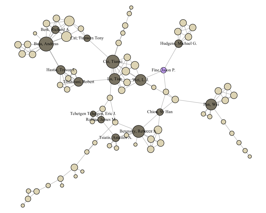
Figure 4: The largest connected component of Community 2 in the collaboration network.

Figure 5 shows the largest connected component of Community 5 in the collaboration network. The representative nodes in this community include Professor Fan, Jinqing from Princeton University, Professor Li, Runze from Pennsylvania State University, Professor Zou, Hui from University of Minnesota, Professor Tsai, Chih-Ling from University of California Davis, and others. In addition, we find many interesting phenomena, further validating the effectiveness of our method. For example, Professors Fan, Li, and Zou form a loop, indicating that they collaborate very closely. Professor Ma, Shuangge and Professor Huang, Jian, along with others, are relatively closely connected, appearing to form a sub-community. Professor Leng, Chenlei from the University of Warwick serves as a bridge in this community, connecting the group represented by Professor Qin, Jing from Hong Kong Polytechnic University. From the perspective of research directions, the authors in this community all specialize in high-dimensional fields.

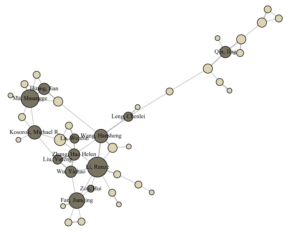
Figure 5: The largest connected component of Community 5 in the collaboration network.

The last community we want to discuss is Community 10. As shown in Figure 6, the visualization of Community 10 reveals that the nodes within this community are very closely connected. The density of this community is 21.2%, much higher than that of Community 2 (5.5%) and Community 5 (9.3%). This suggests that the collaboration among the authors in this community is more close. The representative authors of this community, Professors Ibrahim, Joseph G., Zhu, Hongtu, and Styner, Martin A. are all from the University of North Carolina at Chapel Hill, which are renowned statisticians. It is very interesting that both Professor Ibrahim, Joseph G. and Professor Zhu, Hongtu are the Ph.D. advisors of Professor Shi Xiaoyan. Additionally, there are many higher-order complete sub-network structures in this community, where every pair of distinct nodes is connected by an edge. For example, a four-node complete sub-graph is formed by Professor Ibrahim, Joseph G., Professor Sinha, Debajyoti, Professor Lipsitz, Stuart R., and Professor Fitzmaurice, Garrett A., which further indicates that this community is highly collaborative.

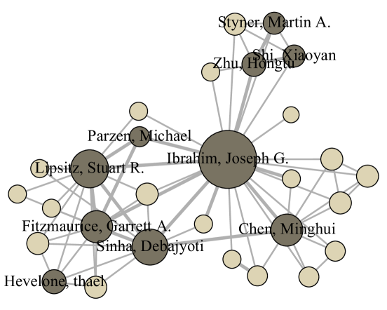
Figure 6: The largest connected component of Community 10 in the collaboration network.

5.4 Comparison with Other Methods

To demonstrate that utilizing the bipartite network brings improvements, we compare the results of our newly proposed BASIC method with SCORE (Jin, 2015) and SCORE+ (Jin et al., 2021). The SCORE method essentially performs community detection using only the primary network, while SCORE+ builds on SCORE by applying pre-PCA normalization and Laplacian transformation to the adjacency matrix and considering an additional eigenvector for clustering. The subplots on the top left, bottom left and bottom right of Figure 7 show the different community detection results by BASIC and SCORE, respectively. Nodes in different communities are assigned different colors. In general, BASIC and SCORE exhibited more balanced community sizes, while the largest community in SCORE+ accounted for 68.7% of the total number of nodes. We find that SCORE+ is not suitable for our collaboration network. This is because SCORE+ requires that the $K$-th eigenvalue is very close to the $(K+1)$-th eigenvalue, while there is a relatively large gap between the $(K+1)$-th and $(K+2)$-th eigenvalues. However, as shown in Table 3, in the collaboration network studied in this paper, not only the $K$-th and $(K+1)$-th eigenvalues but even the $(K+2)$-th eigenvalue are very close, making it difficult to argue that considering one additional eigenvector would bring a significant improvement. Therefore, the SCORE+ method does not apply well to our collaboration network. By incorporating additional structural information into the collaboration network, we are able to achieve better results than SCORE+.

Table 3: Variation of $1-{\hat{\lambda}_{K+1}}/{\hat{\lambda}_{K}}$in our collaboration network as $K$ varies from 1 to 16. Note that the number of communities in our collaboration network is 12.

$K$	1	2	3	4	5	6	7	8
$1-{\hat{\lambda}_{K+1}}/{\hat{\lambda}_{K}}$	0.098	0.105	0.093	0.062	0.004	0.097	0.046	0.006
$K$	9	10	11	12	13	14	15	16
$1-{\hat{\lambda}_{K+1}}/{\hat{\lambda}_{K}}$	0.045	0.051	0.019	0.011	0.012	0.020	0.004	0.012

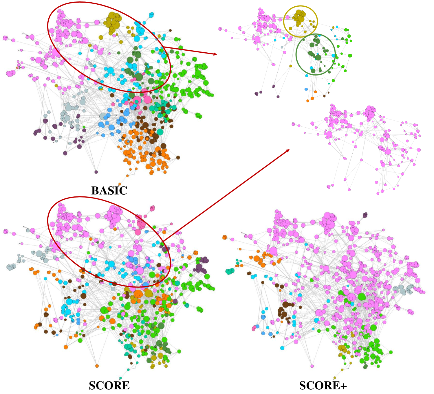
Figure 7: Top Left: Community detection results using the BASIC method; Top Right: Community detection results of part of selected nodes using the BASIC and SCORE methods. Bottom Left: Community detection results using the SCORE method; Bottom Right: Community detection results using the SCORE+ method; The nodes from different communities are assigned different colors.

In comparison of BASIC and SCORE, we observe that SCORE categorizes 55% of the top 20 most cited authors into the same community. In contrast, BASIC shows more balanced communities than SCORE. To provide a clearer comparison of the differences between BASIC and SCORE, the subplot on the top right shows the community structure of the selected nodes. Visually, these nodes exhibit distinct community structures, but the SCORE method groups all of them into the same community. In contrast, our BASIC method divides them into three main communities. Specifically, the yellow node community within the yellow circle of Figure 7 consists mainly of authors from KU Leuven and Hasselt University in Belgium. The community corresponding to the green nodes within the green circle is the highly connected Community 10 mentioned above. In addition, SCORE assigns Professors Fine, Jason P., and Wei, Lee-Jen to two different communities. However, Professor Wei, Lee-Jen supervises the doctoral studies of Professor Fine, Jason P., and they collaborate closely. In contrast, BASIC assigns them to the same community and groups them with professors from Harvard University.

6 Conclusion

In this paper, we propose a Bipartite Assisted Spectral-clustering approach for Identifying Communities (BASIC). It incorporates bipartite network information to community structure learning in social network analysis. By introducing an aggregated squared adjacency matrix, BASIC effectively takes into account the bipartite information without distorting the primary network structure. We systematically study the theoretical properties of BASIC, and demonstrate its privilege across various scenarios of simulation studies. Furthermore, we collect a large-scale academic network dataset from the statistics field, with author collaboration network being our primary interest. We also construct three bipartite networks - author-paper, author-institution, and author-region, from the collected data. Then we explore the community structure of the collaboration network using BASIC, leading to numerous intriguing findings.

Appendix A Figure

Figure 8 shows the scree plot of the primary collaboration network.

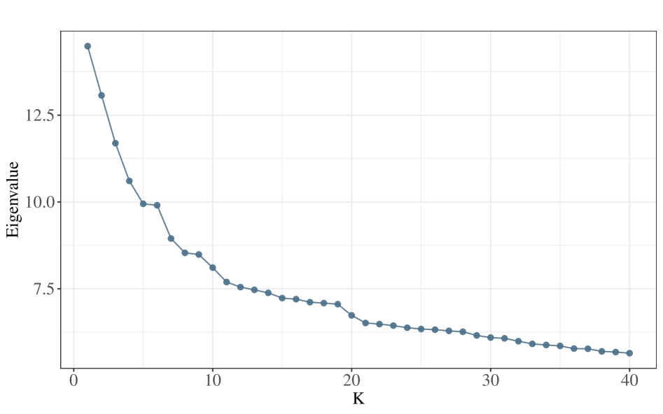
Figure 8: The scree plot of the primary collaboration network

Appendix B Proof

B.1 Proof of Proposition 1

Proof  Recall that the mean structure of aggregated matrix $\boldsymbol{\Omega}_{M}\equiv\left\|\boldsymbol{\theta}\right\|^{2}\left\|\boldsymbol{\delta}\right\|^{2}\boldsymbol{\Theta}_{\theta}\bar{\mathbf{S}}\boldsymbol{\Theta}_{\theta}^{\top}$ as shown in (4). We first explicitly describe the eigen-structure of $\boldsymbol{\Omega}_{M}$. Based on this and symmetry of $\bar{\mathbf{S}}$ and assume its first $K$ eigenvalues are nonzero, it can be decomposed as $\bar{\mathbf{S}}=\mathbf{J}\boldsymbol{\Sigma}\mathbf{J}^{\top}$, where $\boldsymbol{\Sigma}\in\mathbb{R}^{K\times K}$ is a diagonal matrix with positive eigenvalues arranged in descending order, and columns in $\mathbf{J}=\left[\mathbf{{j}}_{1},\mathbf{{j}}_{2},\ldots,\mathbf{{j}}_{K}\right]\in\mathbb{R}^{K\times K}$ are the corresponding eigenvectors. Substituting $\bar{\mathbf{S}}=\mathbf{J}\boldsymbol{\Sigma}\mathbf{J}^{\top}$ into (4), we can obtain:

$$\boldsymbol{\Omega}_{M}=\|\boldsymbol{\theta}\|^{2}\|\boldsymbol{\delta}\|^{2}\left(\boldsymbol{\Theta}_{\theta}\mathbf{J}\right)\boldsymbol{\Sigma}\left(\boldsymbol{\Theta}_{\theta}\mathbf{J}\right)^{\top}.$$ (8)

We can verify that $\boldsymbol{\Theta}_{\theta}\mathbf{J}$ is orthonormal as $\boldsymbol{\Theta}_{\theta}$ and $\mathbf{J}$ are both orthonormal matrices. Therefore, (8) is an eigenvalue decomposition of $\boldsymbol{\Omega}_{M}$, we rewrite it as $\boldsymbol{\Omega}_{M}=\mathbf{U}\boldsymbol{\Lambda}\mathbf{U}^{\top}$, where

$$\boldsymbol{\Lambda}=\|\boldsymbol{\theta}\|^{2}\|\boldsymbol{\delta}\|^{2}\boldsymbol{\Sigma},$$ (9)

$$\mathbf{U}=\boldsymbol{\Theta}_{\boldsymbol{\theta}}\mathbf{J}.$$ (10)

To view (9), $\boldsymbol{\Omega}_{M}$ has $K$ non-zero eigenvalues with

$$\lambda_{i}(\boldsymbol{\Omega}_{M})=\|\boldsymbol{\theta}\|^{2}\|\boldsymbol{\delta}\|^{2}\lambda_{i}(\boldsymbol{\Sigma})=\|\boldsymbol{\theta}\|^{2}\|\boldsymbol{\delta}\|^{2}\lambda_{i}(\boldsymbol{\bar{\mathbf{S}}})\text{ for }1\leqslant i\leqslant K,$$

which gives (5). In addition, each row of (10) can be rewritten as $({{\theta}_{i}}/{\|\boldsymbol{\theta}^{\left(l_{i}\right)}\|})\mathbf{J}_{\bar{l_{i}}}$, giving (6). Moreover, recall $\mathbf{J}$ is a square and orthogonal matrix, and we have $\left\|\mathbf{U}_{\bar{\boldsymbol{i}}}\right\|=\left\|({{\theta}_{i}}/{\|\boldsymbol{\theta}^{\left(l_{i}\right)}\|})\mathbf{J}_{\bar{l_{i}}}\right\|={{\theta}_{i}}/{\|\boldsymbol{\theta}^{\left(l_{i}\right)}\|}$, implying $\left\|\mathbf{U}_{\bar{\boldsymbol{i}}}\right\|\asymp{{\theta}_{i}}/{\|\boldsymbol{\theta}\|}$.

 

B.2 Proof of Lemma 1

Proof  Denote the empirical version of the aggregated adjacency matrix as $\mathbf{M}=\mathbf{A}\mathbf{A}^{\top}+\sum_{q=1}^{Q}\mathbf{B}^{(q)}\mathbf{B}^{(q)\top}$. For notation simplicity, we rewrite $\mathbf{A}$ as $\mathbf{B}^{(0)}$, then $\mathbf{M}=\sum_{q=0}^{Q}\mathbf{B}^{(q)}\mathbf{B}^{(q)\top}$. By definition, we obtain,

$$\mathbf{M} =\sum_{q=0}^{Q}\left(\boldsymbol{\Omega}^{(q)}+\mathbf{W}^{(q)}\right)\left(\boldsymbol{\Omega}^{(q)}+\mathbf{W}^{(q)}\right)^{\top}$$

$$=\sum_{q=0}^{Q}\boldsymbol{\Omega}^{(q)}\boldsymbol{\Omega}^{(q)\top}+\sum_{q=0}^{Q}\boldsymbol{\Omega}^{(q)}\mathbf{W}^{(q)\top}+\sum_{q=0}^{Q}\mathbf{W}^{(q)}\boldsymbol{\Omega}^{(q)\top}+\sum_{q=0}^{Q}\mathbf{W}^{(q)}\mathbf{W}^{(q)\top}$$

$$=\boldsymbol{\Omega}_{M}+\sum_{q=0}^{Q}\boldsymbol{\Omega}^{(q)}\mathbf{W}^{(q)\top}+\sum_{q=0}^{Q}\mathbf{W}^{(q)}\boldsymbol{\Omega}^{(q)\top}+\sum_{q=0}^{Q}\mathbf{W}^{(q)}\mathbf{W}^{(q)\top}.$$

This gives

$$\left\|\mathbf{M}-\boldsymbol{\Omega}_{M}\right\|=\left\|\sum_{q=0}^{Q}\boldsymbol{\Omega}^{(q)}\mathbf{W}^{(q)\top}+\sum_{q=0}^{Q}\mathbf{W}^{(q)}\boldsymbol{\Omega}^{(q)\top}+\sum_{q=0}^{Q}\mathbf{W}^{(q)}\mathbf{W}^{(q)\top}\right\|$$ (11)

$$\leqslant 2\sum_{q=0}^{Q}\left\|\boldsymbol{\Omega}^{(q)}\right\|\left\|\mathbf{W}^{(q)}\right\|+\sum_{q=0}^{Q}\left\|\mathbf{W}^{(q)}\right\|^{2}$$

$$\leqslant 2\left\|\boldsymbol{\theta}\right\|\left\|\boldsymbol{\delta}\right\|\sum_{q=1}^{Q}\left\|\mathbf{S}^{(q)}\right\|\left\|\mathbf{W}^{(q)}\right\|+2\left\|\boldsymbol{\theta}\right\|^{2}\left\|\mathbf{S}^{(0)}\right\|\left\|\mathbf{W}^{(0)}\right\|+\sum_{q=0}^{Q}\left\|\mathbf{W}^{(q)}\right\|^{2}$$

$$= 2\left\|\boldsymbol{\theta}\right\|\left\|\boldsymbol{\delta}\right\|\sum_{q=1}^{Q}\sigma_{\max}\left(\mathbf{S}^{(q)}\right)\sigma_{\max}\left(\mathbf{W}^{(q)}\right)+\left\|\boldsymbol{\theta}\right\|^{2}\sigma_{\max}\left(\mathbf{S}^{(0)}\right)\sigma_{\max}\left(\mathbf{W}^{(0)}\right)$$

$$+\sum_{q=0}^{Q}\sigma_{\max}\left(\mathbf{W}^{(q)}\right)^{2},$$

where the second equality is directly from the definitions of $\boldsymbol{\Omega}^{(q)},q=0,1,\ldots,Q$.

Next, our goal is to give an upper bound of the right-hand side of Equation (11). By Assumption 2, without loss of generality, we assume $\sigma_{\max}(\mathbf{F}^{(q)})\gg\sqrt{\log(n)Z}/(\left\|\boldsymbol{\theta}\right\|\left\|\boldsymbol{\delta}\right\|)$, then

$$\min(\left\|\boldsymbol{\theta}\right\|\left\|\boldsymbol{\delta}\right\|,\left\|\boldsymbol{\theta}\right\|^{2})\sigma_{\max}(\mathbf{S}^{(q)})\gtrsim\left\|\boldsymbol{\theta}\right\|\left\|\boldsymbol{\delta}\right\|(\sigma_{\min}(\boldsymbol{\Psi}_{\theta}))^{2}\sigma_{\max}(\mathbf{F}^{(q)})$$ (12)

$$\gtrsim \left\|\boldsymbol{\theta}\right\|\left\|\boldsymbol{\delta}\right\|\sigma_{\max}(\mathbf{F}^{(q)})\gg\sqrt{\log(n)Z}\gtrsim\max_{q=0}^{Q}\sigma_{\max}(\mathbf{W}^{(q)}),$$

where the first and second inequality are directly from Assumption 3, the third inequality is from Assumption 2 and last inequality is from Lemma A.2 in Wang et al. (2020), which shows $\max_{q=0}^{Q}\sigma_{\max}(\mathbf{W}^{(q)})\lesssim\sqrt{\log(n)Z}$ with probability at least $1-o\left(n^{-4}\right)$. Otherwise, we can show $\left\|\boldsymbol{\theta}\right\|^{2}\sigma_{\max}\left(\mathbf{S}^{(0)}\right)\sigma_{\max}\left(\mathbf{W}^{(0)}\right)\gg\max_{q=0}^{Q}\sigma_{\max}\left(\mathbf{W}^{(q)}\right)$ similarly. Therefore, by (12), we can obtain

$$\left\|\mathbf{M}-\boldsymbol{\Omega}_{M}\right\|\lesssim\left\|\boldsymbol{\theta}\right\|\left\|\boldsymbol{\delta}\right\|\sqrt{\log(n)Z}\max\left\{\max_{q=1}^{Q}\sigma_{\max}\left(\mathbf{F}^{(q)}\right),\lambda_{\max}(\mathbf{E})\right\}$$

with probability at least $1-o\left(n^{-4}\right)$.  

B.3 Proof of Theorem 1

First, we provide two key results.

Lemma 2

For the ratio matrix $\mathbf{{R}}\in\mathbb{R}^{n\times(K-1)}$ derived from the eigenvectors of the population aggregated adjacency matrix $\boldsymbol{\Omega}_{\mathbf{M}}$, then for all $1\leqslant i_{1}\leqslant n$ and $1\leqslant i_{2}\leqslant n$, the following inequalities hold:

$$\left\|\mathbf{R}_{\bar{i_{1}}}-\mathbf{R}_{\bar{i_{2}}}\right\|\geqslant 2 \quad\text{if}\quad l_{i_{1}}\neq l_{i_{2}},$$

$$\left\|\mathbf{R}_{\bar{i_{1}}}-\mathbf{R}_{\bar{i_{2}}}\right\|=0 \quad\text{if}\quad l_{i_{1}}=l_{i_{2}},$$

where $l_{i}$ represents the community label of node $i$.

Proposition 2

Under Assumptions 1, 2 and 3, for the ratio matrix $\mathbf{R}$ and $\hat{\mathbf{R}}$, for $n$ large enough, with probability at least $1-o\left(n^{-4}\right)$, we have

$$\|\hat{\mathbf{R}}-\mathbf{R}\|_{F}^{2}\lesssim\frac{\log(n)ZT_{n}^{2}}{\theta_{\min}^{2}\left\|\boldsymbol{\theta}\right\|^{4}}\left(\frac{\max\left\{\max_{q=1}^{Q}\sigma_{\max}\left(\mathbf{F}^{(q)}\right),\lambda_{\max}(\mathbf{E})\right\}}{\sum_{q=1}^{Q}\sigma^{2}_{\min}\left(\mathbf{F}^{(q)}\right)+\lambda^{2}_{\min}\left(\mathbf{E}\right)}\right)^{2},$$ (13)

where $Z=\max\left(\theta_{\max},\delta_{\max}\right)\max\left(\|\boldsymbol{\theta}\|_{1},\|\boldsymbol{\delta}\|_{1}\right)$ and $T_{n}=\log(n)$.

The proofs of these two results defer to the end of this appendix. Now we focus on the main result.

Proof  We aim to bound the distance between $\mathbf{N}^{*}$ and the ratio matrix $\mathbf{{R}}$ constructed from the eigenvectors of the expected aggregated adjacency matrix $\boldsymbol{\Omega}_{M}$. By the definition of the matrix $\mathbf{N}^{*}=\underset{\mathbf{N}\in\mathcal{N}_{n,k-1,K}}{\operatorname{argmin}}\|\mathbf{N}-\hat{\mathbf{R}}\|_{F}^{2}$. Note that $\mathcal{N}_{n,K-1,K}$ denotes the set of $n\times(K-1)$ matrices with only $K$ different rows. Recall that $\mathbf{R}$ is also a $n\times(K-1)$ matrices with only $K$ different rows, thus $\mathbf{R}\in\mathcal{N}_{n,K-1,K}$. We can get $\|\mathbf{N}^{*}-\hat{\mathbf{R}}\|\leqslant\|\mathbf{R}-\hat{\mathbf{R}}\|$. Then, we obtain

$$\left\|\mathbf{N}^{*}-\mathbf{R}\right\|_{F}^{2} \leqslant\|\mathbf{N}^{*}-\hat{\mathbf{R}}+\hat{\mathbf{R}}-\mathbf{R}\|_{F}^{2}\lesssim\|\mathbf{N}^{*}-\hat{\mathbf{R}}\|_{F}^{2}+\|\hat{\mathbf{R}}-\mathbf{R}\|_{F}^{2}$$

$$\lesssim\|\mathbf{R}-\hat{\mathbf{R}}\|_{F}^{2}+\|\hat{\mathbf{R}}-\mathbf{R}\|_{F}^{2}\quad\text{(by $\|\mathbf{N}^{*}-\hat{\mathbf{R}}\|\leqslant\|\mathbf{R}-\hat{\mathbf{R}}\|$)}$$

$$\lesssim\|\mathbf{R}-\hat{\mathbf{R}}\|_{F}^{2}$$

$$\lesssim\frac{\log(n)ZT_{n}^{2}}{\theta_{\min}^{2}\left\|\boldsymbol{\theta}\right\|^{4}}\left(\frac{\max\left\{\max_{q=1}^{Q}\sigma_{\max}\left(\mathbf{F}^{(q)}\right),\lambda_{\max}(\mathbf{E})\right\}}{\sum_{q=1}^{Q}\sigma^{2}_{\min}\left(\mathbf{F}^{(q)}\right)+\lambda^{2}_{\min}\left(\mathbf{E}\right)}\right)^{2}\quad\text{(by Proposition~\ref{Proposition3})},$$

where $Z=\max\left(\theta_{\max},\delta_{\max}\right)\max\left(\|\boldsymbol{\theta}\|_{1},\|\boldsymbol{\delta}\|_{1}\right)$, and $T_{n}=\log(n)$.

Define $\mathcal{W}\equiv\{1\leqslant i\leqslant$ $\left.n:\left\|\mathbf{N}_{\bar{i}}^{*}-\mathbf{R}_{\bar{i}}\right\|\leqslant\frac{1}{2}\right\}$. Assume that nodes $i_{1}$ and $i_{2}$ belong to different communities in the set $\mathcal{W}$, i.e., $l_{i_{1}}\neq l_{i_{2}}$. According to Lemma 2, we have $\|\mathbf{R}_{\bar{i_{1}}}-\mathbf{R}_{\bar{i_{2}}}\|\geqslant 2$. We can obtain that for $\bar{i_{1}},\bar{i_{2}}\in\mathcal{W}$,

$$\left\|\mathbf{N}_{\bar{i_{1}}}^{*}-\mathbf{N}_{\bar{i_{2}}}^{*}\right\| =\left\|\mathbf{N}_{\bar{i_{1}}}^{*}-\mathbf{R}_{\bar{i_{1}}}+\mathbf{R}_{\bar{i_{1}}}-\mathbf{R}_{\bar{i_{2}}}+\mathbf{R}_{\bar{i_{2}}}-\mathbf{N}_{\bar{i_{2}}}^{*}\right\|$$

$$\geqslant\left\|\mathbf{R}_{\bar{i_{1}}}-\mathbf{R}_{\bar{i_{2}}}\right\|-\left\|\mathbf{N}_{\bar{i_{1}}}^{*}-\mathbf{R}_{\bar{i_{1}}}+\mathbf{R}_{\bar{i_{2}}}-\mathbf{N}_{\bar{i_{2}}}^{*}\right\|$$

$$\geqslant\left\|\mathbf{R}_{\bar{i_{1}}}-\mathbf{R}_{\bar{i_{2}}}\right\|-\left\|\mathbf{N}_{\bar{i_{1}}}^{*}-\mathbf{R}_{\bar{i_{1}}}\right\|-\left\|\mathbf{N}_{\bar{i_{2}}}^{*}-\mathbf{R}_{\bar{i_{2}}}\right\|$$

$$\geqslant 2-\frac{1}{2}-\frac{1}{2}=1\quad\text{(by the definition of $\mathcal{W}$)}.$$

Then, by the same deduction as Theorem 1 in Wang et al. (2020), we can show

$$|\mathcal{V}\backslash\mathcal{W}|\lesssim \frac{\log(n)ZT_{n}^{2}}{\theta_{\min}^{2}\left\|\boldsymbol{\theta}\right\|^{4}}\left(\frac{\max\left\{\max_{q=1}^{Q}\sigma_{\max}\left(\mathbf{F}^{(q)}\right),\lambda_{\max}(\mathbf{E})\right\}}{\sum_{q=1}^{Q}\sigma^{2}_{\min}\left(\mathbf{F}^{(q)}\right)+\lambda^{2}_{\min}\left(\mathbf{E}\right)}\right)^{2}$$

$$= \frac{\log(n)ZT_{n}^{2}}{\theta_{\min}^{2}\left\|\boldsymbol{\theta}\right\|^{4}}(\operatorname{SNR}^{\operatorname{BASIC}})^{-2}.$$

 

B.4 Proof of Lemma 2

By the definition of the ratio matrix $\mathbf{{R}}$, we can obtain that

$$\left\|\mathbf{R}_{\bar{i_{1}}}-\mathbf{R}_{\bar{i_{2}}}\right\|^{2} =\left\|\frac{\left(\mathbf{U}_{2\sim K}\mathbf{O}_{\mathbf{U}^{\prime}}\right)_{\bar{i_{1}}}}{C_{U}\mathbf{u}_{1}(i_{1})}-\frac{\left(\mathbf{U}_{2\sim K}\mathbf{O}_{\mathbf{U}^{\prime}}\right)_{\bar{i_{2}}}}{C_{U}\mathbf{u}_{1}(i_{2})}\right\|^{2}$$

$$=\left\|\frac{\left(\mathbf{U}_{2\sim K}\right)_{\bar{i_{1}}}}{\mathbf{u}_{1}(i_{1})}-\frac{\left(\mathbf{U}_{2\sim K}\right)_{\bar{i_{2}}}}{\mathbf{u}_{1}(i_{2})}\right\|^{2}+\left\|\frac{\mathbf{u}_{1}(i_{1})}{\mathbf{u}_{1}(i_{1})}-\frac{\mathbf{u}_{1}(i_{2})}{\mathbf{u}_{1}(i_{2})}\right\|^{2}$$

$$=\left\|\frac{\mathbf{U}_{\bar{i_{1}}}}{\mathbf{u}_{1}(i_{1})}-\frac{\mathbf{U}_{\bar{i_{2}}}}{\mathbf{u}_{1}(i_{2})}\right\|^{2}$$

$$=\left\|\frac{\mathbf{J}_{\bar{l_{i_{1}}}}}{\mathbf{J}_{\bar{l_{i_{1}}}}(1)}-\frac{\mathbf{J}_{\bar{l_{i_{2}}}}}{\mathbf{J}_{\bar{l_{i_{2}}}}(1)}\right\|^{2}\quad\text{(by Proposition~\ref{Proposition1})}.$$

Therefore, if $l_{i_{1}}=l_{i_{2}}$, we have $\mathbf{J}_{\bar{l_{i_{1}}}}=\mathbf{J}_{\bar{l_{i_{2}}}}$, thus, $\left\|\mathbf{R}_{\bar{i_{1}}}-\mathbf{R}_{\bar{i_{2}}}\right\|^{2}=0$. On the other hand, if $l_{i_{1}}\neq l_{i_{2}}$, by noting Proposition 1, it is seen that the matrix $\mathbf{J}$ is orthogonal matrix, thus $\left\|\mathbf{J}\right\|=1$ and $\left\langle\mathbf{J}_{\bar{l_{i_{1}}}},\mathbf{J}_{\bar{l_{i_{2}}}}\right\rangle=0$ for $i_{1}\neq i_{2}$. Thus, if $l_{i_{1}}\neq l_{i_{2}}$, we have $\left\|\mathbf{R}_{\bar{i_{1}}}-\mathbf{R}_{\bar{i_{2}}}\right\|^{2}=1/{|\mathbf{J}_{\bar{l_{i_{1}}}}(1)|}+{1}/{|\mathbf{J}_{\bar{l_{i_{2}}}}(1)|}\geqslant 1+1=2$.

Appendix C Proof of Proposition 2

We first provide some lemmas that facilitate technical proofs.

Lemma 3

Let the first $K$ leading eigenvectors of $\mathbf{M}$ as $\hat{\mathbf{U}}=\left[\hat{\mathbf{u}}_{1},\hat{\mathbf{u}}_{2},\ldots,\hat{\mathbf{u}}_{K}\right]\in\mathbb{R}^{n\times K}$, and the first $K$ leading eigenvectors of $\boldsymbol{\Omega}_{M}$ as ${\mathbf{U}}=\left[\mathbf{{u}}_{1},\mathbf{{u}}_{2},\ldots,\mathbf{{u}}_{K}\right]\in\mathbb{R}^{n\times K}$. Under Assumption 3 and 2, there exist an orthogonal matrix $\mathbf{O}_{\mathbf{U}}\in\mathbb{R}^{(K-1)\times(K-1)}$ and a constant $C_{U}\in\{-1,1\}$, such that for $n$ large enough, with probability at least $1-o\left(n^{-4}\right)$, the following bounds hold

$$\max\left\{\|\hat{\mathbf{U}}_{2\sim K}-\mathbf{U}_{2\sim K}\mathbf{O}_{\mathbf{U}}\|_{F},\|\hat{\mathbf{u}}_{1}-\mathbf{u}_{1}C_{U}\|_{F}\right\}$$ (14)

$$\lesssim \frac{\sqrt{\log(n)Z}}{\left\|\boldsymbol{\theta}\right\|^{2}}\left(\frac{\max\left\{\max_{q=1}^{Q}\sigma_{\max}\left(\mathbf{F}^{(q)}\right),\lambda_{\max}(\mathbf{E})\right\}}{\sum_{q=1}^{Q}\sigma^{2}_{\min}\left(\mathbf{F}^{(q)}\right)+\lambda^{2}_{\min}\left(\mathbf{E}\right)}\right),$$

where $Z=\max\left(\theta_{\max},\delta_{\max}\right)\max\left(\|\boldsymbol{\theta}\|_{1},\|\boldsymbol{\delta}\|_{1}\right)$.

Proof  By applying Lemma 5.1 in Lei and Rinaldo (2015) and Lemma 4 in Wang et al. (2020), there exists an orthogonal matrix $\mathbf{O}_{\mathbf{U}}\in\mathbb{R}^{(K-1)\times(K-1)}$, the distance (defined in Frobenius norm) between eigenvectors of aggregated square matrix $\mathbf{M}$ and its population version $\boldsymbol{\Omega}_{M}$ is bounded by spectral norm of noise matrix, i.e.,

$$\max\left\{\|\hat{\mathbf{U}}_{2\sim K}-\mathbf{U}_{2\sim K}\mathbf{O}_{\mathbf{U}}\|_{F},\|\hat{\mathbf{u}}_{1}-\mathbf{u}_{1}C_{\mathbf{U}}\|_{F}\right\}$$ (15)

$$\leqslant \frac{2\sqrt{2K}}{\min\left\{\lambda_{\min}(\boldsymbol{\Omega}_{M}),\lambda_{1}(\boldsymbol{\Omega}_{M})-\lambda_{2}(\boldsymbol{\Omega}_{M})\right\}}\left\|\mathbf{M}-\boldsymbol{\Omega}_{M}\right\|$$

$$\leqslant \frac{2\sqrt{2K}}{\lambda_{\min}(\boldsymbol{\Omega}_{M})}\left\|\mathbf{M}-\boldsymbol{\Omega}_{M}\right\|,$$

where the last inequality is based on the same deduction as (A.15) in Wang et al. (2020). Additionally, $K$ is assumed to be independent of $n$ and it is a constant. By Lemma 1, we can obtain that with probability $1-O(n^{-4})$,

$$\max\left\{\|\hat{\mathbf{U}}_{2\sim K}-\mathbf{U}_{2\sim K}\mathbf{O}_{\mathbf{U}}\|_{F},\|\hat{\mathbf{u}}_{1}-\mathbf{u}_{1}C_{\mathbf{U}}\|_{F}\right\}$$ (16)

$$\lesssim \frac{\left\|\mathbf{M}-\boldsymbol{\Omega}_{M}\right\|}{\lambda_{\min}\left(\sum_{q=1}^{Q}\boldsymbol{\Omega}^{(q)}\boldsymbol{\Omega}^{(q)\top}\right)}$$

$$\lesssim \frac{\left\|\boldsymbol{\theta}\right\|\left\|\boldsymbol{\delta}\right\|\sqrt{\log(n)Z}\max\left\{\max_{q=1}^{Q}\sigma_{\max}\left(\mathbf{F}^{(q)}\right),\lambda_{\max}(\mathbf{E})\right\}}{\left\|\boldsymbol{\theta}\right\|^{2}\left\|\boldsymbol{\delta}\right\|^{2}\sum_{q=1}^{Q}\sigma^{2}_{\min}\left(\mathbf{S}^{(q)}\right)+\left\|\boldsymbol{\theta}\right\|^{4}\sigma^{2}_{\min}\left(\mathbf{S}^{(0)}\right)}$$

$$\lesssim \frac{\sqrt{\log(n)Z}}{\left\|\boldsymbol{\theta}\right\|^{2}}\left(\frac{\max\left\{\max_{q=1}^{Q}\sigma_{\max}\left(\mathbf{F}^{(q)}\right),\lambda_{\max}(\mathbf{E})\right\}}{\sum_{q=1}^{Q}\sigma^{2}_{\min}\left(\mathbf{F}^{(q)}\right)+\lambda^{2}_{\min}\left(\mathbf{E}\right)}\right),$$

where the second inequality we use the fact that

$$\lambda_{\min}\left(\sum_{q=0}^{Q}\boldsymbol{\Omega}^{(q)}\boldsymbol{\Omega}^{(q)\top}\right)\geq \sum_{q=0}^{q}\lambda_{\min}\left(\boldsymbol{\Omega}^{(q)}\boldsymbol{\Omega}^{(q)\top}\right)$$

$$= \left\|\boldsymbol{\theta}\right\|^{2}\left\|\boldsymbol{\delta}\right\|^{2}\sum_{q=1}^{Q}\sigma^{2}_{\min}\left(\mathbf{S}^{(q)}\right)+\left\|\boldsymbol{\theta}\right\|^{4}\sigma^{2}_{\min}\left(\mathbf{S}^{(0)}\right),$$

and Proposition 1, and the last inequality is from Assumption 3 where $\|\boldsymbol{\theta}\|\asymp\|\boldsymbol{\delta}\|$.  

For a constant $0<C<1$, we define $\mathcal{V}_{U}\equiv\left(1\leqslant i\leqslant n;\left|\frac{\hat{\mathbf{u}}_{1}(i)}{C_{U}\mathbf{u}_{1}(i)}-1\right|\leqslant C\right)$.

Lemma 4

For the nodes in $\mathcal{V}_{U}$, we have the following equations hold,

$$\left|\hat{\mathbf{u}}_{1}(i)\right|\asymp\left|C_{U}\mathbf{u}_{1}(i)\right|\asymp\frac{{\theta}_{i}}{\|\boldsymbol{\theta}\|}\quad\text{for}\quad i\in\mathcal{V}_{U}.$$

Moreover, with a probability of at least $1-O\left(n^{-4}\right)$, the cardinalities of $\mathcal{V}\backslash\mathcal{V}_{U}$ satisfies

$$\left|\mathcal{V}\backslash\mathcal{V}_{U}\right|\lesssim\frac{\log(n)Z}{\theta_{\min}^{2}\left\|\boldsymbol{\theta}\right\|^{4}}\left(\frac{\max\left\{\max_{q=1}^{Q}\sigma_{\max}\left(\mathbf{F}^{(q)}\right),\lambda_{\max}(\mathbf{E})\right\}}{\sum_{q=1}^{Q}\sigma^{2}_{\min}\left(\mathbf{F}^{(q)}\right)+\lambda^{2}_{\min}\left(\mathbf{E}\right)}\right)^{2}.$$

Proof  For the first part, we first show that the elements in the leading eigenvector of $\mathbf{U}$ are all positive. To see this, we only need to show $C\leqslant\mathbf{j}_{1}(i)\leqslant 1$ for a constant $C>0$. Then by the Expression (10), we can get the desired results. Note that $\mathbf{j}_{1}$ is the leading eigenvector of $\bar{\mathbf{S}}$, based on Lemma 7 in Wang et al. (2020), what we need to show is that $\bar{\mathbf{S}}$ is irreducible and non-negative. By definition,

$$\bar{\mathbf{S}}= \sum_{q=1}^{Q}(\mathbf{S}^{(q)}\mathbf{S}^{(q)\top})+(\|\boldsymbol{\theta}\|^{2}/\|\boldsymbol{\delta}\|^{2})\mathbf{S}^{(0)}\mathbf{S}^{(0)\top}$$

$$= \boldsymbol{\Psi}_{\boldsymbol{\theta}}\sum_{q=1}^{Q}(\mathbf{F}^{(q)}\mathbf{F}^{(q)\top})\boldsymbol{\Psi}_{\boldsymbol{\theta}}+(\|\boldsymbol{\theta}\|^{2}/\|\boldsymbol{\delta}\|^{2})\boldsymbol{\Psi}_{\boldsymbol{\theta}}(\mathbf{E}\mathbf{E}^{\top})\boldsymbol{\Psi}_{\boldsymbol{\theta}}.$$

By Assumption 1, all terms on the right hand side are irreducible, thus $\bar{\mathbf{S}}$ is also irreducible. Moreover, by noting $\mathbf{F}^{(q)}(i,j)\geq 0$ and $\mathbf{E}(i_{1},i_{2})\geq 0$, we can show that $\bar{\mathbf{S}}$ is nonnegative. Thus, we conclude the result.

Now we show the first part, recall that $\mathbf{U}_{\bar{i}}={({\theta}_{i}}/{\|\boldsymbol{\theta}^{\left(l_{i}\right)}\|})\mathbf{J}_{\bar{l_{i}}}$ as shown in Proposition 1, we can obtain $\left|C_{U}\mathbf{u}_{1}(i)\right|=\left|C_{U}{({\theta}_{i}}/{\|\boldsymbol{\theta}^{(l_{i})}\|})\mathbf{j}_{1}\left(l_{i}\right)\right|$ for $1\leqslant i\leqslant n$. Combine $\|\boldsymbol{\theta}\|^{2}=\sum_{k=1}^{K}\|\boldsymbol{\theta}^{(k)}\|^{2}$ and Assumption 3, we can get $\|\boldsymbol{\theta}^{(i)}\|\asymp\|\boldsymbol{\theta}\|$ for $1\leqslant i\leqslant K$. Noting that $0<C\leqslant\mathbf{J}_{1}(i)\leqslant 1$ for $1\leqslant i\leqslant n$, which is proved above. The following equation holds,

$$\left|C_{U}\mathbf{u}_{1}(i)\right|=\left|C_{U}\frac{{\theta}_{i}}{\|\boldsymbol{\theta}^{(l_{i})}\|}\mathbf{j}_{1}\left(l_{i}\right)\right|\asymp\left|\frac{{\theta}_{i}}{\|\boldsymbol{\theta}\|}\right|\quad\text{ for }\quad 1\leqslant i\leqslant n.$$ (17)

Then, for $i\in\mathcal{V}_{U}$, we have $\left|\frac{\hat{\mathbf{u}}_{1}(i)}{C_{U}\mathbf{u}_{1}(i)}-1\right|\leqslant C<1$, thus $\left|\hat{\mathbf{u}}_{1}(i)\right|\asymp\left|C_{U}\mathbf{u}_{1}(i)\right|$, where $\left|C_{U}\right|=1$ by Proposition 1. Substituting to Equation (17), we obtain

$$\left|\hat{\mathbf{u}}_{1}(i)\right|\asymp\left|C_{U}\mathbf{u}_{1}(i)\right|\asymp\left|\frac{{\theta}_{i}}{\|\boldsymbol{\theta}\|}\right|,\quad\text{ for }\quad i\in\mathcal{V}_{U}.$$ (18)

Furthermore, by Equation (18), we can obtain $\left|C_{U}\mathbf{u}_{1}(i)\right|\asymp|{{\theta}_{i}}/{\|\boldsymbol{\theta}\|}>0$ for $1\leqslant i\leqslant n$, which means that $C_{U}\mathbf{u}_{1}(i)$ can be used as a denominator. Thus, we have

$$\sum_{i\in\mathcal{V}\backslash\mathcal{V}_{U}}\left(\frac{\hat{\mathbf{u}}_{1}(i)}{C_{U}\mathbf{u}_{1}(i)}-1\right)^{2}=\sum_{i\in\mathcal{V}\backslash\mathcal{V}_{U}}\left(\frac{1}{C_{U}\mathbf{u}_{1}(i)}\right)^{2}\left(\hat{\mathbf{u}}_{1}(i)-C_{U}\mathbf{u}_{1}(i)\right)^{2}$$ (19)

$$\leqslant \sum_{i\in\mathcal{V}\backslash\mathcal{V}_{U}}\frac{\|\boldsymbol{\theta}\|^{2}}{\theta_{\min}^{2}}\left(\hat{\mathbf{u}}_{1}(i)-C_{U}\mathbf{u}_{1}(i)\right)^{2}\quad\text{(by Equation \eqref{Pro_6:App_5})}$$

$$\leqslant \sum_{i=1}^{n}\frac{\|\boldsymbol{\theta}\|^{2}}{\theta_{\min}^{2}}\left(\hat{\mathbf{u}}_{1}(i)-C_{U}\mathbf{u}_{1}(i)\right)^{2}\leqslant\frac{\|\boldsymbol{\theta}\|^{2}}{\theta_{\min}^{2}}\left\|\hat{\mathbf{u}}_{1}-\mathbf{u}_{1}C_{U}\right\|^{2}$$

$$\leqslant \frac{\log(n)Z}{\theta_{\min}^{2}\left\|\boldsymbol{\theta}\right\|^{4}}\left(\frac{\max\left\{\max_{q=1}^{Q}\sigma_{\max}\left(\mathbf{F}^{(q)}\right),\lambda_{\max}(\mathbf{E})\right\}}{\sum_{q=1}^{Q}\sigma^{2}_{\min}\left(\mathbf{F}^{(q)}\right)+\lambda^{2}_{\min}\left(\mathbf{E}\right)}\right)^{2}\quad\text{(by Proposition~\ref{Proposition2})}.$$

Therefore, there exists a constant $C$, the nodes in $\mathcal{V}\backslash\mathcal{V}_{U}$ satisfy $\left(\frac{\hat{\mathbf{u}}_{1}(i)}{C_{U}\mathbf{u}_{1}(i)}-1\right)^{2}>C^{2}$. By Equation (19), we have

$$\left|\mathcal{V}\backslash\mathcal{V}_{U}\right|= \sum_{i\in\mathcal{V}\backslash\mathcal{V}_{U}}1\leqslant\sum_{\mathcal{V}\backslash\mathcal{V}_{U}}\frac{1}{C^{2}}\left(\frac{\hat{\mathbf{u}}_{1}(i)}{C_{U}\mathbf{u}_{1}(i)}-1\right)^{2}$$

$$\lesssim \frac{\log(n)Z}{\theta_{\min}^{2}\left\|\boldsymbol{\theta}\right\|^{4}}\left(\frac{\max\left\{\max_{q=1}^{Q}\sigma_{\max}\left(\mathbf{F}^{(q)}\right),\lambda_{\max}(\mathbf{E})\right\}}{\sum_{q=1}^{Q}\sigma^{2}_{\min}\left(\mathbf{F}^{(q)}\right)+\lambda^{2}_{\min}\left(\mathbf{E}\right)}\right)^{2}.$$

 

The following inequality is taken from Appendix A.7.5 in Wang et al. (2020).

Lemma 5

For $\mathbf{v},\mathbf{u}\in\mathbf{R}^{n},a,b\in\mathbf{R},a>0,b>0$, the following inequality holds, $\left\|\frac{\mathbf{v}}{a}-\frac{\mathbf{u}}{b}\right\|^{2}\leqslant 2\left(\frac{1}{a^{2}}\|\mathbf{v}-\mathbf{u}\|^{2}+\frac{(b-a)^{2}}{(ab)^{2}}\|\mathbf{u}\|^{2}\right)$.

Next, we turn to prove the main result of Proposition 2. By the definition of $\mathbf{R}$, we have

$$\left\|\left(\mathbf{R}\right)_{\bar{i}}\right\|^{2}= \left\|\frac{\left(\mathbf{U}_{2\sim K}\mathbf{O}_{\mathbf{U}}\right)_{\bar{i}}}{C_{U}\mathbf{u}_{1}(i)}\right\|^{2}\leqslant\frac{\frac{{\theta}^{2}_{i}}{\|\boldsymbol{\theta}\|^{2}}}{(\mathbf{u}_{1}(i))^{2}}\lesssim\frac{\frac{{\theta}^{2}_{i}}{(\boldsymbol{\theta})^{2}}}{\frac{{\theta}^{2}_{i}}{\|\boldsymbol{\theta}^{(l_{i})}\|^{2}}(\mathbf{j}_{1}\left(l_{i}\right))^{2}}\leqslant C,$$ (20)

where the first inequality is from $\left\|\left(\mathbf{U}_{2\sim K}\mathbf{O}_{\mathbf{U}}\right)_{\bar{i}}\right\|=\left\|\left(\mathbf{U}_{2\sim K}\right)_{\bar{i}}\right\|\leq\left\|\mathbf{U}_{\bar{i}}\right\|\leq\frac{{\theta}^{2}_{i}}{\|\boldsymbol{\theta}\|^{2}}$, the second inequality is from (6), and the last inequality is from $0<C^{-1/2}\leq\mathbf{j}_{1}\left(l_{i}\right)$. Next, dividing the nodes into two distinct sets $\mathcal{V}_{U}$ and $\mathcal{V}\backslash\mathcal{V}_{U}$, we can see

$$\|\hat{\mathbf{R}}-\hat{\mathbf{R}}\|_{F}^{2}=\sum_{i\in\mathcal{V}\backslash\mathcal{V}_{U}}\|\hat{\mathbf{R}}_{\bar{i}}-{\mathbf{R}}_{\bar{i}}\|^{2}+\sum_{i\in\mathcal{V}_{U}}\|\hat{\mathbf{R}}_{\bar{i}}-{\mathbf{R}}_{\bar{i}}\|^{2}.$$ (21)

We bound two terms on the right hand side separately. For the first term in Equation (21), we can show

$$\sum_{i\in\mathcal{V}\backslash\mathcal{V}_{U}}\|\hat{\mathbf{R}}_{\bar{i}}-{\mathbf{R}}_{\bar{i}}\|^{2}\leqslant C\sum_{i\in\mathcal{V}\backslash\mathcal{V}_{U}}\left(\|\hat{\mathbf{R}}_{\bar{i}}\|^{2}+\|\mathbf{R}_{\bar{i}}\|^{2}\right)$$ (22)

$$\leqslant C\sum_{i\in\mathcal{V}\backslash\mathcal{V}_{U}}\left(KT_{n}^{2}+C\right)\quad\text{(by the definition of $\hat{\mathbf{R}}$ and \eqref{App_3:equ_11})}$$

$$\leqslant C\left|\mathcal{V}\backslash\mathcal{V}_{U}\right|T_{n}^{2}$$

$$\lesssim \frac{\log(n)ZT_{n}^{2}}{\theta_{\min}^{2}\left\|\boldsymbol{\theta}\right\|^{4}}\left(\frac{\max\left\{\max_{q=1}^{Q}\sigma_{\max}\left(\mathbf{F}^{(q)}\right),\lambda_{\max}(\mathbf{E})\right\}}{\sum_{q=1}^{Q}\sigma^{2}_{\min}\left(\mathbf{F}^{(q)}\right)+\lambda^{2}_{\min}\left(\mathbf{E}\right)}\right)^{2}\quad\text{(by Lemma~\ref{Lemma3}).}$$

For the second term in Equation 21, we can get that

$$\sum_{i\in\mathcal{V}_{U}}\left\|\hat{\mathbf{R}}_{\bar{i}}-\mathbf{R}_{\bar{i}}\right\|^{2}$$ (23)

$$\leqslant C\sum_{i\in\mathcal{V}_{U}}\left\|\frac{\left(\hat{\mathbf{U}}_{2\sim K}\right)_{\bar{i}}}{\hat{\mathbf{u}}_{1}(i)}-\frac{\left(\mathbf{U}_{2\sim K}\mathbf{O}_{\mathbf{U}^{\prime}}\right)_{\bar{i}}}{C_{U}\mathbf{u}_{1}(i)}\right\|^{2}\quad\text{(by the definition of $\hat{\mathbf{R}}$, ${\mathbf{R}}$ and Lemma~\ref{Lemma4})}$$

$$\leqslant C\sum_{i\in\mathcal{V}_{U}}\left(\frac{1}{\left(\hat{\mathbf{u}}_{1}(i)\right)^{2}}\left\|\left(\hat{\mathbf{U}}_{2\sim K}\right)_{\bar{i}}-\left(\mathbf{U}_{2\sim K}\mathbf{O}_{\mathbf{U}^{\prime}}\right)_{\bar{i}}\right\|^{2}+\frac{\left(C_{V}\mathbf{u}_{1}(i)-\hat{\mathbf{u}}_{1}(i)\right)^{2}}{\left(\hat{\mathbf{u}}_{1}(i)C_{U}\mathbf{u}_{1}(i)\right)^{2}}\left\|\left(\mathbf{U}_{2\sim K}\mathbf{O}_{\mathbf{U}^{\prime}}\right)_{\bar{i}}\right\|^{2}\right)$$

$$\leqslant C\sum_{i\in\mathcal{V}_{U}}\left(\frac{\|\boldsymbol{\theta}\|^{2}}{\boldsymbol{\theta}_{i}^{2}}\left\|\left(\hat{\mathbf{U}}_{2\sim K}\right)_{\bar{i}}-\left(\mathbf{U}_{2\sim K}\mathbf{O}_{\mathbf{U}^{\prime}}\right)_{\bar{i}}\right\|^{2}+\frac{\|\boldsymbol{\theta}\|^{2}}{\boldsymbol{\theta}_{i}^{2}}\left(C_{U}\mathbf{u}_{1}(i)-\hat{\mathbf{u}}_{1}(i)\right)^{2}\right)\quad\text{(by Lemma~\ref{Lemma3})}$$

$$\leqslant C\frac{\|\boldsymbol{\theta}\|^{2}}{\theta_{\min}^{2}}\left(\sum_{i\in\mathcal{V}_{U}}\left\|\left(\hat{\mathbf{U}}_{2\sim K}\right)_{\bar{i}}-\left(\mathbf{U}_{2\sim K}\mathbf{O}_{\mathbf{U}^{\prime}}\right)_{\bar{i}}\right\|^{2}+\sum_{i\in\mathcal{V}_{U}}\left(C_{U}\mathbf{u}_{1}(i)-\hat{\mathbf{u}}_{1}(i)\right)^{2}\right)$$

$$\leqslant C\frac{\|\boldsymbol{\theta}\|^{2}}{\theta_{\min}^{2}}\left(\left\|\hat{\mathbf{U}}_{2\sim K}-\mathbf{U}_{2\sim K}\mathbf{O}_{\mathbf{U}^{\prime}}\right\|_{F}^{2}+\left\|\hat{\mathbf{u}}_{1}-\mathbf{u}_{1}C_{U}\right\|_{F}^{2}\right)$$

$$\leqslant \frac{\log(n)Z}{\theta_{\min}^{2}\left\|\boldsymbol{\theta}\right\|^{4}}\left(\frac{\max\left\{\max_{q=1}^{Q}\sigma_{\max}\left(\mathbf{F}^{(q)}\right),\lambda_{\max}(\mathbf{E})\right\}}{\sum_{q=1}^{Q}\sigma^{2}_{\min}\left(\mathbf{F}^{(q)}\right)+\lambda^{2}_{\min}\left(\mathbf{E}\right)}\right)^{2}\quad\text{(by Proposition~\ref{Proposition2})}.$$

Combining Equation (22) and Equation (23), we can obtain that

$$\|\hat{\mathbf{R}}-\mathbf{R}\|_{F}^{2}\lesssim\frac{\log(n)ZT_{n}^{2}}{\theta_{\min}^{2}\left\|\boldsymbol{\theta}\right\|^{4}}\left(\frac{\max\left\{\max_{q=1}^{Q}\sigma_{\max}\left(\mathbf{F}^{(q)}\right),\lambda_{\max}(\mathbf{E})\right\}}{\sum_{q=1}^{Q}\sigma^{2}_{\min}\left(\mathbf{F}^{(q)}\right)+\lambda^{2}_{\min}\left(\mathbf{E}\right)}\right)^{2},$$

where $Z=\max\left(\theta_{\max},\delta_{\max}\right)\max\left(\|\boldsymbol{\theta}\|_{1},\|\boldsymbol{\delta}\|_{1}\right)$, and $T_{n}=\log(n)$.

References

- Adamic and Glance (2005) Lada A Adamic and Natalie Glance. The political blogosphere and the 2004 US election: divided they blog. In Proceedings of the 3rd International Workshop on Link Discovery, pages 36–43, 2005.
- Airoldi et al. (2008) Edo M Airoldi, David Blei, Stephen Fienberg, and Eric Xing. Mixed membership stochastic blockmodels. In Advances in Neural Information Processing Systems, volume 21. Curran Associates, Inc., 2008. URL https://proceedings.neurips.cc/paper_files/paper/2008/file/8613985ec49eb8f757ae6439e879bb2a-Paper.pdf.
- Ding et al. (2023) Yi Ding, Rui Pan, Yan Zhang, and Bo Zhang. A matrix completion bootstrap method for estimating scale-free network degree distribution. Knowledge-Based Systems, 277:110803, 2023.
- Dong et al. (2023) Ang Dong, Shuang Wu, Jincan Che, Yu Wang, and Rongling Wu. Idopnetwork: A network tool to dissect spatial community ecology. Methods in Ecology and Evolution, 14(9):2272–2283, 2023.
- Frobenius (1912) Georg Frobenius. Über matrizen aus nicht negativen elementen. Sitzungsberichte der Königlich Preußischen Akademie der Wissenschaften zu Berlin, pages 456–477, 1912.
- Girvan and Newman (2002) Michelle Girvan and Mark EJ Newman. Community structure in social and biological networks. Proceedings of the National Academy of Sciences, 99(12):7821–7826, 2002.
- Holland et al. (1983) Paul W Holland, Kathryn Blackmond Laskey, and Samuel Leinhardt. Stochastic blockmodels: first steps. Social Networks, 5(2):109–137, 1983.
- Huang et al. (2020) Jinyu Huang, Yani Hou, and Yuansong Li. Efficient community detection algorithm based on higher-order structures in complex networks. Chaos: An Interdisciplinary Journal of Nonlinear Science, 30(2):023114, 2020.
- Hubert and Arabie (1985) Lawrence Hubert and Phipps Arabie. Comparing partitions. Journal of Classification, 2:193–218, 1985.
- Ji and Jin (2016) Pengsheng Ji and Jiashun Jin. Coauthorship and citation networks for statisticians. The Annals of Applied Statistics, 10(4):1779 – 1812, 2016.
- Ji et al. (2022) Pengsheng Ji, Jiashun Jin, Zheng Tracy Ke, and Wanshan Li. Co-citation and co-authorship networks of statisticians. Journal of Business & Economic Statistics, 40(2):469–485, 2022.
- Jin (2015) Jiashun Jin. Fast community detection by score. Annals of Statistics, 43(1):57–89, 2015.
- Jin et al. (2017) Jiashun Jin, Zheng Tracy Ke, and Shengming Luo. Estimating network memberships by simplex vertex hunting. arXiv preprint arXiv:1708.07852, 2017.
- Jin et al. (2021) Jiashun Jin, Zheng Tracy Ke, and Shengming Luo. Improvements on score, especially for weak signals. Sankhya A, 84(1):127–162, March 2021. ISSN 0976-8378. doi: 10.1007/s13171-020-00240-1. URL http://dx.doi.org/10.1007/s13171-020-00240-1.
- Jin et al. (2023) Jiashun Jin, Zheng Tracy Ke, Shengming Luo, and Minzhe Wang. Optimal estimation of the number of network communities. Journal of the American Statistical Association, 118(543):2101–2116, 2023.
- Karrer and Newman (2011) Brian Karrer and Mark EJ Newman. Stochastic blockmodels and community structure in networks. Physical Review E, 83(1):016107, 2011.
- Larremore et al. (2014) Daniel B Larremore, Aaron Clauset, and Abigail Z Jacobs. Efficiently inferring community structure in bipartite networks. Physical Review E, 90(1):012805, 2014.
- Lei and Rinaldo (2015) Jing Lei and Alessandro Rinaldo. Consistency of spectral clustering in stochastic block models. The Annals of Statistics, 43(1):215–237, 2015.
- Li et al. (2020) Tianxi Li, Elizaveta Levina, and Ji Zhu. Network cross-validation by edge sampling. Biometrika, 107(2):257–276, 2020.
- Miao and Li (2023) Ruizhong Miao and Tianxi Li. Informative core identification in complex networks. Journal of the Royal Statistical Society Series B: Statistical Methodology, 85(1):108–126, 2023.
- Miething et al. (2016) Alexander Miething, Ylva B Almquist, Viveca Östberg, Mikael Rostila, Christofer Edling, and Jens Rydgren. Friendship networks and psychological well-being from late adolescence to young adulthood: a gender-specific structural equation modeling approach. BMC Psychology, 4:1–11, 2016.
- Newman (2008) Mark Newman. The physics of networks. Physics Today, 61(11):33–38, 2008.
- Newman (2001) Mark EJ Newman. Scientific collaboration networks. I. Network construction and fundamental results. Physical Review E, 64(1):016131, 2001.
- Newman (2012) Mark EJ Newman. Communities, modules and large-scale structure in networks. Nature Physics, 8(1):25–31, 2012.
- Paul et al. (2023) Subhadeep Paul, Olgica Milenkovic, and Yuguo Chen. Higher-order spectral clustering under superimposed stochastic block models. Journal of Machine Learning Research, 24(320):1–58, 2023.
- Perron (1907) Oskar Perron. Zur theorie der matrizen. Mathematische Annalen, 64(2):248–263, 1907. doi: 10.1007/BF01449896.
- Tian et al. (2016) Zhao Tian, Limin Jia, Honghui Dong, Fei Su, and Zundong Zhang. Analysis of urban road traffic network based on complex network. Procedia Engineering, 137:537–546, 2016.
- Wang and Rohe (2016) S. Wang and K. Rohe. Discussion of “coauthorship and citation networks for statisticians”. The Annals of Applied Statistics, 10(4):1820–1826, 2016.
- Wang et al. (2020) Zhe Wang, Yingbin Liang, and Pengsheng Ji. Spectral algorithms for community detection in directed networks. The Journal of Machine Learning Research, 21(1):6101–6145, 2020.
- Wu et al. (2023) Shuang Wu, Xiang Liu, Ang Dong, Claudia Gragnoli, Christopher Griffin, Jie Wu, Shing-Tung Yau, and Rongling Wu. The metabolomic physics of complex diseases. Proceedings of the National Academy of Sciences, 120(42):e2308496120, 2023.
- Xu et al. (2023) Shirong Xu, Yaoming Zhen, and Junhui Wang. Covariate-assisted community detection in multi-layer networks. Journal of Business & Economic Statistics, 41(3):915–926, 2023.
- Yen and Larremore (2020) Tzu-Chi Yen and Daniel B Larremore. Community detection in bipartite networks with stochastic block models. Physical Review E, 102(3):032309, 2020.
- Yu and Zhu (2024) X Yu and J Zhu. Network community detection using higher-order structures. Biometrika, 111(3):903–923, 2024.
- Zachary (1977) Wayne W Zachary. An information flow model for conflict and fission in small groups. Journal of Anthropological Research, 33(4):452–473, 1977.
- Zhang et al. (2023) Yan Zhang, Rui Pan, Hansheng Wang, and Haibo Su. Community detection in attributed collaboration network for statisticians. Stat, 12(1):e507, 2023.
- Zhang et al. (2020) Yuan Zhang, Elizaveta Levina, and Ji Zhu. Detecting overlapping communities in networks using spectral methods. SIAM Journal on Mathematics of Data Science, 2(2):265–283, 2020.