Two-stage Deep Denoising with Self-guided Noise Attention for Multimodal Medical Images

Abstract

Medical image denoising is considered among the most challenging vision tasks. Despite the real-world implications, existing denoising methods have notable drawbacks as they often generate visual artifacts when applied to heterogeneous medical images. This study addresses the limitation of the contemporary denoising methods with an artificial intelligence (AI)-driven two-stage learning strategy. The proposed method learns to estimate the residual noise from the noisy images. Later, it incorporates a novel noise attention mechanism to correlate estimated residual noise with noisy inputs to perform denoising in a course-to-refine manner. This study also proposes to leverage a multi-modal learning strategy to generalize the denoising among medical image modalities and multiple noise patterns for widespread applications. The practicability of the proposed method has been evaluated with dense experiments. The experimental results demonstrated that the proposed method achieved state-of-the-art performance by significantly outperforming the existing medical image denoising methods in quantitative and qualitative comparisons. Overall, it illustrates a performance gain of 7.64 in Peak Signal-to-Noise Ratio (PSNR), 0.1021 in Structural Similarity Index (SSIM), 0.80 in DeltaE ($\Delta E$), 0.1855 in Visual Information Fidelity Pixel-wise (VIFP), and 18.54 in Mean Squared Error (MSE) metrics.

I Introduction

Noise in medical images refers to the unexpected transformations of pixel values. Such arbitrary modifications can appear in medical images due to numerous inevitable imaging limitations like stochastic capturing conditions, image acquisition process, and respiratory movement [1, 2]. Nonetheless, the noise in medical images can notably degrade the perceptual quality by incorporating errors and artifacts into the results [3]. As a result, it impacts the performance of image analysis algorithms, such as segmentation, registration, and classification. Despite having numerous real-world implications, medical image denoising is significantly challenging due to variable noise patterns and imaging characteristics of different imaging modalities [4, 5, 6].

Despite the challenges, medical image denoising has drawn significant attention from the vision research community. In the early days, medical image denoising was tackled with classical image processing techniques like non-local self-similarity (NSS) [7], sparse coding [8], and filter-based approaches [9, 10, 11]. Later, medical image-denoising methods have advanced beyond the classical approaches by leveraging deep learning with two learning strategies: i) learning denoising as an image-to-image translation by utilizing numerous deep techniques such as encoder-decoder models [12, 13, 14, 15], adversarial learning, [16, 17, 18] etc. and ii) learning residual noise from noisy images by stacked convolution models[19, 1, 20, 6]. It is worth noting that the learning-based denoising methods have shown promising consequences compared to traditional approaches. Nevertheless, the performance of these learning-based denoising approaches is also limited to specific image modality and fails in reducing high-intensity noise with variable patterns similar to real-world scenarios (Please see Fig.1).

The existing image-to-image denoising methods are susceptible to producing over-smoothing in complex spatial distribution. Oppositely, the residual denoising strategies illustrate visually disturbing artifacts with the desaturated complex structure. The lack of salient details in the enhanced images can substantially affect the medical image analysis. In addition to the visual artifacts, the existing methods also focus on addressing specific noise types (i.e., gaussian noise [1, 20, 19, 6], speckle noise [21, 22, 23], etc.). These noise-centric denoising approaches fail to address variable noise patterns commonly appearing in medical images. However, a generic denoising strategy with a multipattern cross-modal learning strategy can broaden the range of noise reduction for variable noise patterns of medical images. The limitations of existing methods and the widespread advantages of learning generic denoising motivated this study to introduce a robust learning-based denoising method for medical image modalities. Thus, the proposed method can address the real-world medical image-denoising challenges by leveraging the cross-modal information.

This study proposes a novel two-stage strategy to counter the limitation of medical image denoising by learning denoising in a course to refine manner. Stage I of the proposed method estimates the underlying noise pattern [1], while stage II utilizes the estimated noise to refine the results with novel self-guided noise attention. The proposed noise attention block strives to perceive the pixel-level correlation between noisy input and estimated noise to enhance the perceptual quality. Apart from the two-stage network, the proposed study also proposes to utilize multi-modal images [24, 25] to generalize the denoising among numerous image modalities and noise patterns. The feasibility of the proposed method is extensively evaluated in different medical image modalities with dense experiments. The major contribution of the proposed study is as follows:

• A two-stage deep network for learning residual noise and leveraging the estimated noise to reconstruct plausible images

• A novel noise-attention mechanism to perceive pixel-level attention on estimated noise and given images

• Propose to generalize the multi-pattern noise on medical image denoising by leveraging multi-modal images

• Conduct dense experiments and achieve state-of-the-art performance on synthesized and real-world medical images.

The rest of the paper is organized into four sections. Section II details data simulation and learning strategy, Section III analyzes the experimental results, and Section IV concludes this work.

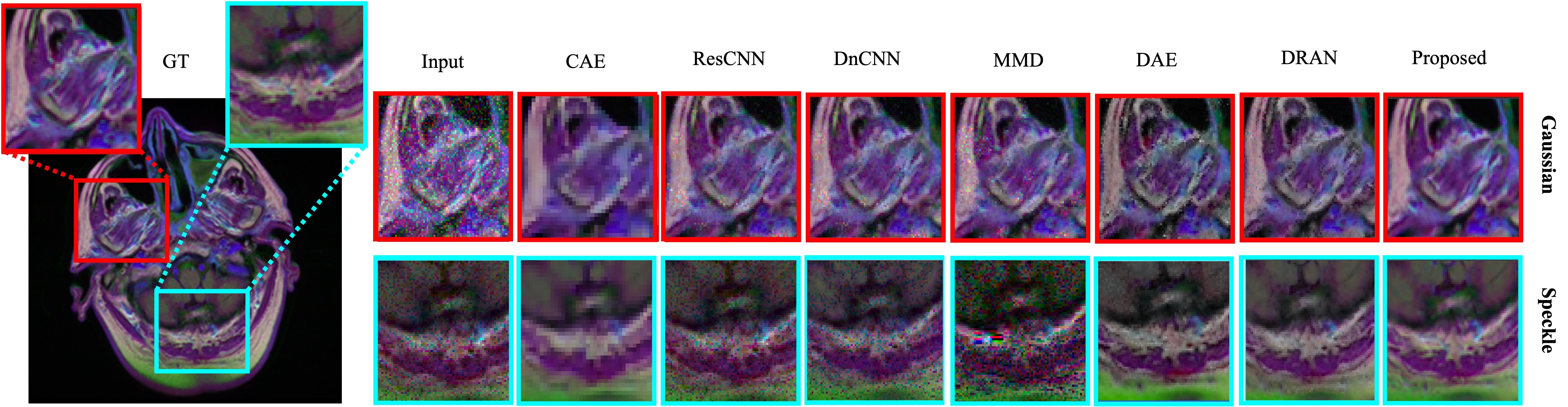
Figure 1: Comparison between deep medical image denoising methods. The existing denoising methods are prone to produce smooth denoising results with visual artifacts. The top row depicts Gaussian denoising; the bottom row shows speckle denoising. In each row, Left to right: GT Image, Noisy Input, CAE [12], ResCNN [20], DnCNN [26], MMD [6], DAE [13], DRAN [1], and the proposed method.

II Method

This study proposes a two-stage novel deep network to learn multi-pattern denoising from multi-modal medical images. This section details the proposed method, including data preparation and evaluation strategies. Fig. 2 illustrates the flowchart of the proposed method.

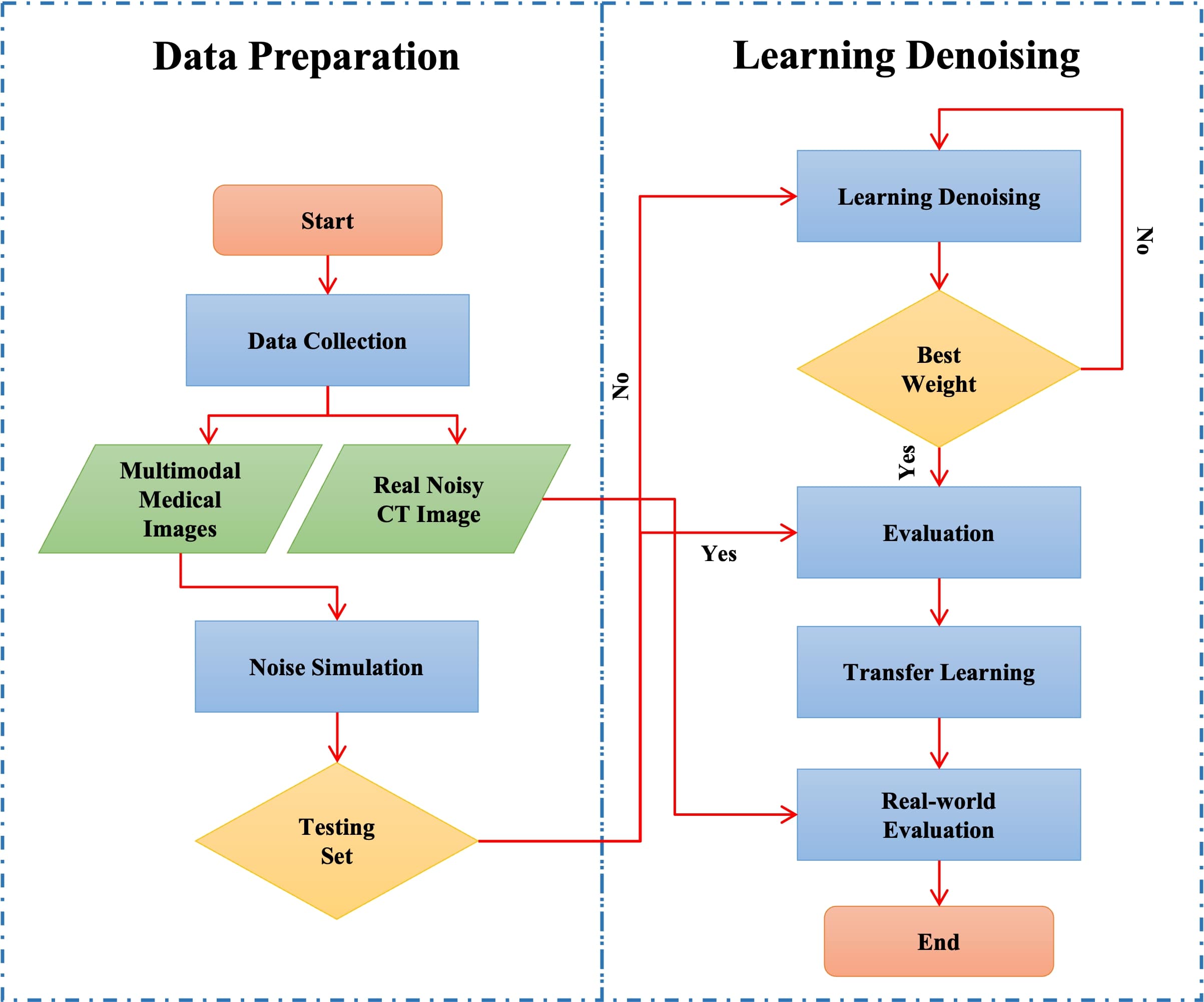
Figure 2: Flowchart of the proposed method. Our proposed method includes data collection and noise simulation strategies. Later, we learned from the collected data and extensively evaluated our method on simulated and real-world noisy medical images.

II-A Data Preparation

Data preparation for any medical image task is known to be a challenging task [27, 1]. Unfortunately, we could not collect any specialized dataset for studying multi-pattern medical image denoising. Therefore, this study introduces a novel algorithm for synthesizing multi-pattern noise on medical images for pair-wise training.

II-A1 Dataset Collection

One of the main objectives of the proposed method is to generalize the medical image denoising among multiple modalities. Therefore, we collected around 30,000 medical images from the open literature before applying the proposed noise-synthesizing algorithm. The collected data samples include multi-modal medical images acquired with different acquisition devices and datasets: i) MRI [28, 29], ii) X-ray [30, 31]), iii) CT images [32, 33], iv) Skin lesion images [34]), and v) Microscopy (i.e., protein atlas [35, 36]). We used 24,000 random images for training and 1,000 images for validation. The remaining 5,000 samples from collected data (1,000 images from each modality) were used for an extensive evaluation with various noise factors.

Apart from the simulated noisy images, we also collected and evaluated our method on real-world noisy CT images (please see section. III-B).

II-A2 Noise Simulation

Noise in medical imaging can vary depending on the image modality and acquisition conditions [1]. Depending on inclusion, noise in medical images can be categorized into two types: additive (i.,e Gaussian noise, impulse noise, quantization noise, etc. ) and multiplicative (speckle noise, poison noise, Rician noise, etc.) [37]. This study proposes generalizing medical image denoising based on their noise inclusion principle. Therefore, we utilized the most common noise patterns, like Gaussian noise from additive and speckle noise from multiplicative category. It is worth noting that other widely studied noise patterns, such as impulse noise, share many common attributes with the Gaussian and speckle noise. For instance, impulse noise introduces random variations in pixel intensities similar to speckle noise, while its inclusion type shares a similar principle as the Gaussian noise. Overall, straight learning of Gaussian and speckle denoising helps us illustrate the feasibility of multi-pattern denoising without incorporating every known noise pattern separately. Such a streamlined strategy has enabled us to assess the performance of existing deep models more efficiently and comprehensively.

We generated an noise (${n}_{s}$) on a given noise-free image ${c}$ as:

$${n}_{s}\sim\mathcal{N}({c}|\mu,\sigma^{2})$$ (1)

$\mu$ and $\sigma^{2}$ represent a noise distribution’s mean and variance ($\mathcal{N}$). We generated the noise pattern for learning denoising using the generated noise distribution.

Simulation of Gaussian Noise: Gaussian noise is known as the most common form of additive noise [1]. Typically, it derived as:

$${I_{N}}={I_{C}}+{n}_{s}$$ (2)

Here, ${I_{C}}$ represents the given clean image.

Simulation of Speckle noise: Speckle noise is the most common form of multiplicative noise observed in medical images. Typically, it is caused by the interaction of light or sound waves with small particles or irregularities in the imaging medium [21]. The speckle noise in medical images can be derived as follows:

$${I_{N}}={I_{C}}+{I_{C}}\times{n}_{s}$$ (3)

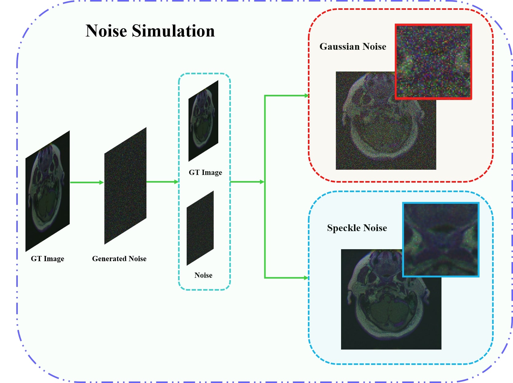
Figure 3: Overview of noisy image generation. The proposed simulation method generates noisy-clean image pairs for training and evaluation.

Based on eqn. 2 and 3, this study proposed to generate the random noise patterns for learning multi-pattern denoising, as shown in Algo. 1. The simulation algorithm generates an arbitrary standard deviation of noise distribution between 0 and 75. This standard deviation has been utilized to generate multi-pattern noise in the given images. Also, the proposed algorithm ensures an even portion of noise patterns in the learning dataset. Notably, such an approach ensures that the generated noise varies in intensity, providing a realistic representation of the noise commonly found in real-world scenarios. Fig. 3 illustrates the sample image-pairs generated by the proposed noise simulation algorithm.

Algorithm 1 Noise simulation in medical image simulation

$Mean$ = 0 - mean for generating random noise

procedure SIMULATION($I_{G},Mean$)

  $Std\leftarrow random(0,75)$ - standard deviation for generating random noise

  $Noise\leftarrow normalDistribution(Mean,Std)$ - generating random noise

  $noisePattern\leftarrow random(0,10)$

  if $noisePattern\%2==0$ then

   $I_{N}\leftarrow I_{G}+Noise$ - generating Gaussian noise

  else

   $I_{N}\leftarrow I_{G}+(I_{G}\times Noise)$ - generating speckle noise   

  return $I_{N}$

II-B Learning Denoising

The medical image denoising is typically handled with the single-stage network. Unlike the previous medical image-denoising methods, this study proposes to leverage a two-stage approach to learn medical image-denoising in a course to refine manner. The proposed method aims to denoise a given noisy medical image as $\mathrm{D}:I_{N}\to I_{C}$. Here, the learning function ($\mathrm{D}$) learns to generate a clean image ($I_{C}$) from a given noisy image ($I_{N}$).

As Fig. 4 illustrates, the learning function ($\mathrm{D}$) comprises two learning stages with two deep networks. The stages of the proposed method aim to perform as follows:

• Stage I: Stage I of the proposed method takes a noisy medical image ($\mathrm{I_{N}}$) and estimates the underlying noise ($\mathrm{N_{E}}$). It comprises a single deep network denoted as a noise estimation network (NEN).

• Stage II: Stage II of the proposed method aims to reconstruct the clean image ($I_{C}$) by leveraging the estimated noise ($\mathrm{N_{E}}$) and the noisy image ($\mathrm{I_{N}}$). Stage II of the proposed method utilizes a novel self-guided noise attention block to estimate the correlation between the noise patterns of the given inputs. It has been denoted as a reconstruction network (RN) in the later section.

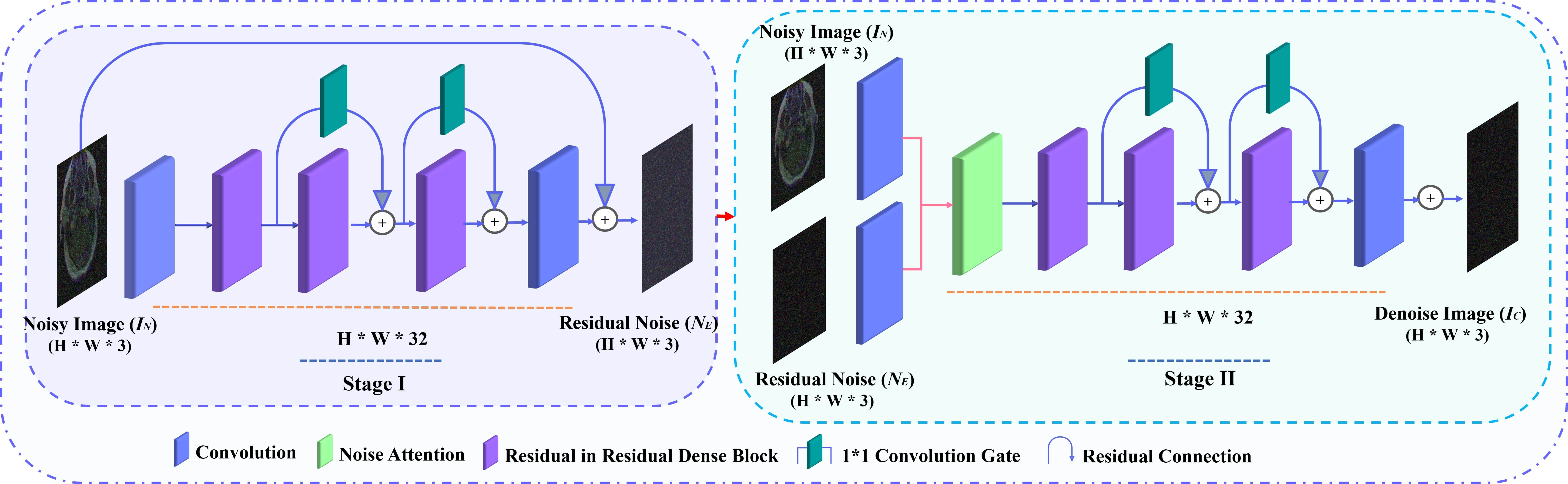
Figure 4: Overview of the proposed two-stage network. Stage I of the proposed method learns to estimate the residual noise, and stage II leverages the estimated noise in refining the denoise outputs.

II-B1 Noise Estimation Network (NEN)

The noisy medical image is typically derived as follows:

$${I_{N}=I_{C}\oplus N}$$ (4)

Here, $\oplus$ represents the types of noise inclusion (i.e., additive or multiplicative), ${I_{N}}$ represents the noisy image, $N$ is the underlying noise, and ${I_{C}}$ is the underlying clean image. The proposed NEN aims to estimate the underlying residual noise ($N_{E}$) from a given noisy medical image ${I_{N}}$ through the mapping function ${\mathrm{F_{E}}:I_{N}\to N_{E}}$. Mapping function ($\mathrm{F_{E}}$) learns the residual noise pattern ($N_{E}$) as $N_{E}\in[0,1]^{H\times W\times 3}$. $H$ and $W$ represent the height and width of the output ($N_{E}$).

To estimate the underlying noise pattern ($N_{E}$), this study leverages consecutive residuals in residual dense blocks (RRDB) [38]. Notably, the RRDB blocks are well known for tackling the gradient vanishing problems. It aims to help the proposed method achieve a deeper architecture by retaining the flow of gradient information. Overall, the RRDB has been pursued as follows:

$$R_{X}=H_{R,d}((H_{R,d-1}(R_{0})))$$ (5)

where $H_{R}$ denotes the residual dense blocks (RDB) [39], and $d$ denotes the operations of the $d^{th}$ RDB, which again can be formulated as follows:

$$R_{d,c}=\tau(H_{d,c}([R_{d-1},R_{d,1},...,R_{c-1}]))$$ (6)

Here $[R_{d-1},R_{d,1},...,R_{c-1}]$ refers to the concatenated feature maps obtained through the $d=5$ number of convolutional layers, $c=8$ denotes the growrate. All convolution layers incorporate the kernel = $3\times 3$, stride = 1, padding = 1, and are activated with the LeakyReLU function. Apart from the RRDB, we leverage the noise gate with $1\times 1$ convolution operation to utilize short-distance residual feature propagation between consecutive RRDB blocks.

Estimating residual noise for denoising has illustrated significant momentum in recent studies. However, denoising based on only residual noises can demonstrate a few drawbacks. For instance, an underestimated residual noise can lead to final output in producing the over-smoothing regions. Similarly, overestimated residual noise is well known for producing over-sharpen final images. Which again can introduce the visual artifacts. This study proposes introducing a secondary learnable network to address the limitation of residual noise estimation.

II-B2 Reconstruction Network (RN)

The proposed RN aims to recover clean medical images ($I_{C}$) by leveraging the estimated noise ($N_{E}$) along with the noisy input image ($I_{N}$) as ${\mathrm{F_{R}}:{I_{N},N_{E}}\to I_{C}}$. The mapping function ($\mathrm{F_{R}}$) learns to generate a clean medical image ($I_{C}$) as $I_{C}\in[0,1]^{H\times W\times 3}$. $H$ and $W$ represent the height of the reconstructed clean image.

Overall, it shares a network architecture similar to NEN. However, unlike the NEN, it takes two inputs: estimated noise ($N_{E}$) and noisy image ($I_{N}$). It applies a standard $3\times 3$ convolution operation to feed the mapped features into the proposed self-guided noise attention block. Later, the attention map of the noise attention block (NOB) propagated into consecutive RRDBs to generate noise-free images [40].

Noise Attention. The proposed novel self-guided NOB intends to accelerate denoising performance. The NOB leverages the estimated noise features and perceives pixel-level attention on the high-intensity noise region as shown in Fig. 5. The noise correlation has been perceived as follows:

$${X_{C}}={C}({N_{T}})\oplus{C}({I_{T}})$$ (7)

Where, $C(\dot{)}$ represents the convolution operation with kernel=3, stride=1, filter=32, $\oplus$ = concatenation, ${N_{T}}$ = estimated feature map of residual noise, and ${I_{T}}$ = convolutional feature of noisy input.

The pixel level spatial attention [41, 42] over concatenated feature map ${X_{C}}$ has been estimated as:

$${A_{C}}={Z_{S}}([{Z_{A}(X)};{Z_{M}(X)}])$$ (8)

Where ${Z_{A}}$ represents the convolution operation with sigmoid activation. Also, ${Z_{A}}$ and ${Z_{M}}$ present the average pooling and max pooling, which generates two 2D feature maps as ${X_{A}}\in\mathbb{R}^{1\times H\times W}$, ${X_{M}}\in\mathbb{R}^{1\times H\times W}$.

The final 32 channels of self-guided noise attention have been perceived as below:

$${S_{A}}={A_{C}}\times{I_{T}}$$ (9)

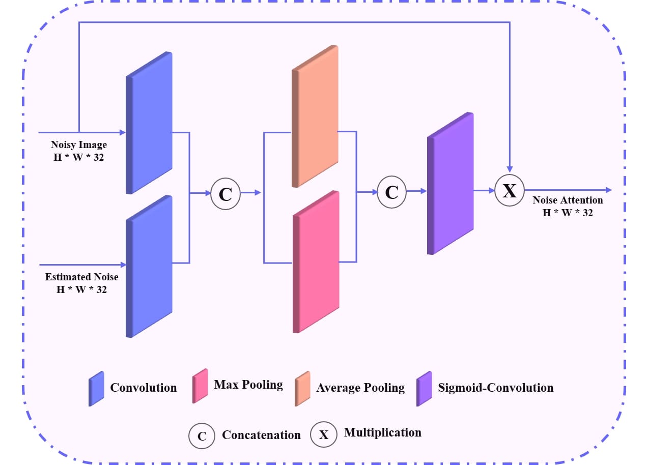
Figure 5: The architecture of the proposed noise attention block. It estimates the pixel-level attention over noisy input with a residual noise pattern.

II-B3 Learning objectives

The proposed NEN and RN are optimized with separate objective functions. The objective of NEN can be derived as follows:

$$W_{E}^{\ast}=\arg{\operatorname*{min}_{W}}\frac{1}{P}\sum_{t=1}^{P}\mathcal{L}_{\mathit{E}}({N_{E}}^{t}),{N_{G}}^{t})$$ (10)

Here, $\mathcal{L}_{\mathit{E}}$ has been set as mean-square-error loss as :

$$\mathcal{L}_{\mathit{E}}=\parallel{N_{G}}-{N_{E}}\parallel_{1}^{2}$$ (11)

Similarly, the objective function of RN aims to minimize the error as follows:

$$W_{R}^{\ast}=\arg{\operatorname*{min}_{W}}\frac{1}{P}\sum_{t=1}^{P}\mathcal{L}_{\mathit{R}}({I_{N}}^{t}),{I_{G}}^{t})$$ (12)

Here, $\mathcal{L}_{\mathit{R}}$ has been set as L1-loss:

$$\mathcal{L}_{\mathit{R}}=\parallel{I_{G}}-{I_{C}}\parallel_{1}$$ (13)

It is worth noting L1 and L2 distances are commonly used as pixel-wise loss functions. However, L2-loss is directly related to the PSNR and tends to produce smoother images [43]. Therefore, an L1 objective function has been considered as a reconstruction loss for the RN throughout this study.

II-B4 Training Details

The proposed two-stage multi-pattern denoising is implemented with the PyTorch framework [44]. The NEN and RN were optimized with an Adam optimizer [45]. The hyperparameters for the optimizer were tuned as $\beta_{1}=0.9$, $\beta_{2}=0.99$, and learning rate = 5e-4. We trained both models for 100 epochs with a constant batch size of 24. During the training process, we generated random patterns with random noise standard deviation. Please see Algorithm. 1 for noise simulation and learning procedure of the proposed method. Notably, such random noise generation techniques help the proposed method in addressing the overfitting until model convergence [46]. It took around 24 hours to converge our model. We conducted our experiments on a machine comprised of an AMD Ryzen 3200G central processing unit (CPU) clocked at 3.6 GHz, a random-access memory of 16 GB, and An Nvidia Geforce GTX 3060 (12GB) graphical processing unit (GPU).

III Experiments and results

The feasibility of the proposed method has been verified with dense experiments. We studied the performance of state-of-the-art medical image denoising methods on five image modalities (i.e., MRI, X-ray, Microscopy, Skin Lesion, and CT) images by incorporating Gaussian and speckle noise with distinct noise levels (i.e., 20, 25, 50, and 75) to each image sample. Further, we assessed the comparing method with qualitative comparison and summarised quantatitive performance [47, 48] with the following evaluation metrics: PSNR, SSIM, DeltaE, VIFP, and MSE. Later, we verified the feasibility of the novel components with ablation experiments.

III-A Comparison with State-of-the-art

We compared the performance of multi-pattern medical image denoising with state-of-the-art residual denoising methods (i.e., ResCNN [20], DnCNN [26], MMD [6], MID-DRAN [1]) and image-to-image translation medical image denoising method (i.e., CAE [12], DAE [13]). All denoising methods have been trained and tested under the same data samples with suggested hyperparameters.

III-A1 MRI

MRI is one of the most widely used medical imaging techniques that uses a powerful magnetic field and radio waves to create detailed images of the inside of the body [49]. MRI is used to diagnose numerous medical conditions, including cancer, heart disease, neurological disorders, and musculoskeletal injuries. Table I illustrates the performance comparison between state-of-the-art deep denoising models and the proposed method for MRI denoising. The proposed two-stage network outperforms the existing denoising method for speckle and Gaussian denoising. It cumulatively outperforms the deep denoising methods by 11.04 in PSNR, 0.0358 in SSIM, 1.67 in $\Delta E$, 0.2843 in VIFP, and 27.62 in MSE metric for speckle denoising. It also illustrates a significant jump in Gaussian denoising by 8.2725 in PSNR, 0.0966 in SSIM, 1.67 in $\Delta E$, 0.2297 in VIFP, and 33.34 in MSE.

Additionally, we compared the deep methods visual comparison, as shown in Fig. 6. It is visible that the proposed method can produce visually plausible images without illustrating noticeable visual artifacts.

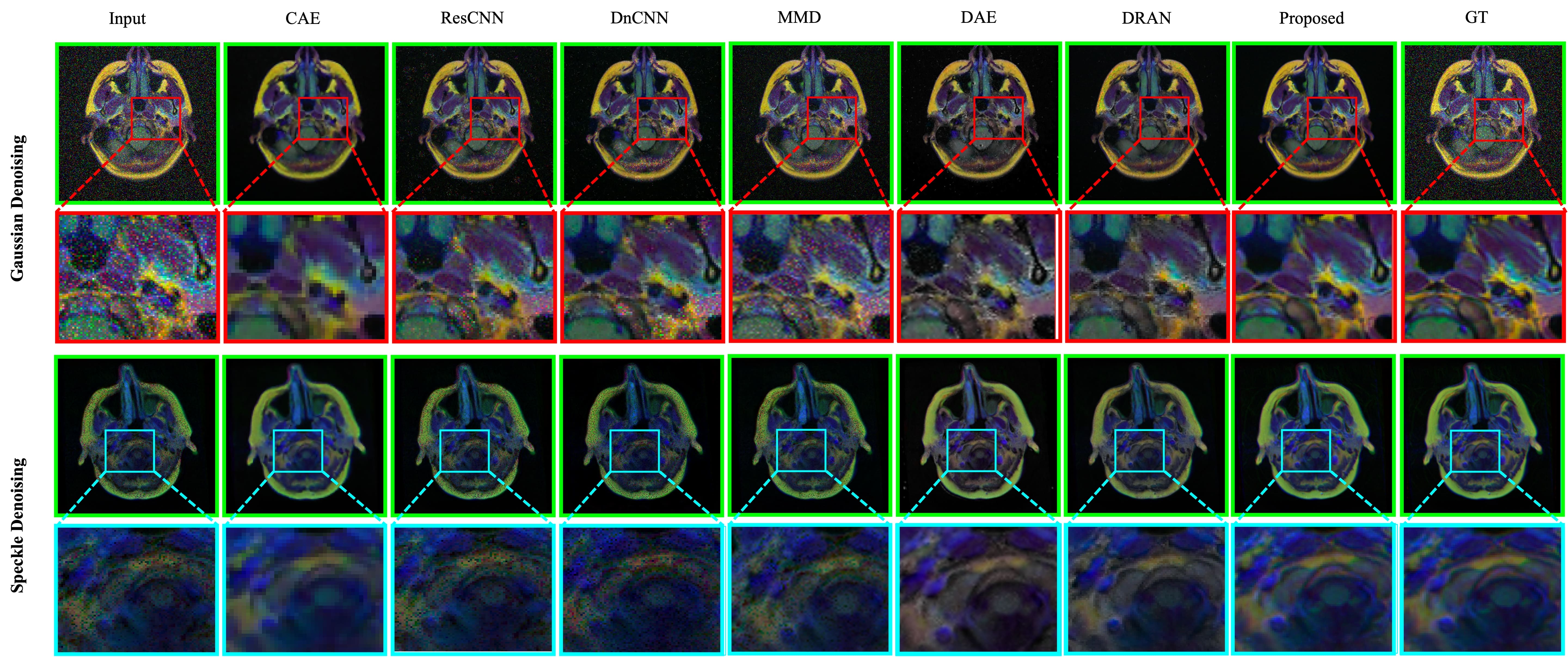
Figure 6: Qualitative comparison for MRI denoising. The proposed method can produce sharper images without incorporating visual artifacts. The top example illustrates Gaussian denoising; the bottom shows speckle denoising. In each row, Left to right: Noisy input, CAE [12], ResCNN [20], DnCNN [26], MMD [6], DAE [13], DRAN [1] [1], proposed method, and ground truth image.

Model	$\sigma$	Gaussian					Speckle					Average
		PSNR	SSIM	$\Delta E$	VIFP	MSE	PSNR	SSIM	$\Delta E$	VIFP	MSE	PSNR	SSIM	$\Delta E$	VIFP	MSE
CAE	10	33.93	0.9375	2.42	0.4071	37.63	33.82	0.9381	2.40	0.4094	38.86	33.87	0.9378	2.41	0.4083	38.24
ResCNN		26.68	0.7517	5.07	0.2261	173.40	24.48	0.6878	6.28	0.1615	298.81	25.58	0.7198	5.68	0.1938	236.11
DnCNN		26.53	0.7131	5.71	0.2197	180.03	25.13	0.6934	6.05	0.1708	256.01	25.83	0.7033	5.88	0.1953	218.02
MMD		28.40	0.8395	3.99	0.5339	191.15	28.40	0.8395	3.99	0.5339	191.15	28.40	0.8395	3.99	0.5339	191.15
DAE		24.88	0.6848	6.33	0.1899	277.58	23.32	0.6280	7.34	0.1471	391.25	24.10	0.6564	6.83	0.1685	334.41
DRAN		35.15	0.9442	2.52	0.5164	28.23	35.49	0.9613	2.18	0.5878	30.00	35.32	0.9528	2.35	0.5521	29.12
Proposed		43.00	0.9851	0.94	0.7208	3.92	50.61	0.9977	0.34	0.9135	0.8800	46.81	0.9914	0.64	0.8172	2.40
CAE	25	33.72	0.9318	2.51	0.3915	38.48	33.93	0.9386	2.38	0.41	37.87	33.83	0.9352	2.45	0.4008	38.18
ResCNN		28.84	0.7704	4.00	0.3069	91.43	24.57	0.6896	6.26	0.1649	290.96	26.70	0.73	5.13	0.2359	191.20
DnCNN		27.82	0.7689	4.46	0.2694	118.41	25.44	0.7079	5.83	0.1823	237.40	26.63	0.7384	5.15	0.2259	177.91
MMD		28.43	0.8379	3.98	0.5309	188.05	28.43	0.8379	3.98	0.5309	188.05	28.43	0.8379	3.98	0.5309	188.05
DAE		27.98	0.7709	4.56	0.2908	134.03	23.53	0.6384	7.11	0.1551	370.02	25.75	0.7047	5.84	0.2229	252.02
DRAN		34.38	0.9270	2.60	0.4799	30.96	35.58	0.9604	2.21	0.5755	29.18	34.98	0.9437	2.40	0.5277	30.07
Proposed		41.77	0.9830	1.03	0.6865	5.54	47.42	0.9958	0.50	0.8677	1.73	44.60	0.9894	0.77	0.7771	3.64
CAE	50	33.28	0.9211	2.67	0.3653	41.62	33.99	0.9387	2.37	0.4091	37.41	33.64	0.9299	2.52	0.3872	39.51
ResCNN		26.75	0.6155	5.14	0.3157	138.83	24.97	0.7032	5.97	0.1778	260.36	25.86	0.6594	5.56	0.2468	199.60
DnCNN		26.83	0.7171	4.01	0.3145	136.33	26.23	0.7438	5.24	0.2097	194.76	26.53	0.7305	4.63	0.2621	165.54
MMD		28.45	0.8343	3.98	0.5215	183.68	28.45	0.8343	3.98	0.5215	183.68	28.45	0.8343	3.98	0.5215	183.68
DAE		26.33	0.6137	5.52	0.3097	156.64	23.90	0.6550	6.73	0.1670	338.20	25.12	0.6343	6.13	0.2384	247.42
DRAN		32.80	0.8756	2.75	0.4337	40.35	35.36	0.9574	2.28	0.5527	29.94	34.08	0.9165	2.52	0.4932	35.15
Proposed		41.09	0.9811	1.10	0.671	6.57	44.55	0.9927	0.69	0.8175	3.21	42.82	0.9869	0.89	0.7443	4.89
CAE	75	32.85	0.9105	2.79	0.3433	45.37	33.97	0.9382	2.38	0.4065	37.55	33.41	0.9244	2.58	0.3749	41.46
ResCNN		20.53	0.2831	12.52	0.2101	580.27	25.53	0.7212	5.61	0.1956	225.80	23.03	0.5022	9.07	0.2029	403.03
DnCNN		21.17	0.3179	11.06	0.2214	498.24	27.00	0.7713	4.77	0.2361	162.06	24.09	0.5446	7.92	0.2288	330.15
MMD		28.45	0.8304	3.98	0.5082	179.87	28.45	0.8304	3.98	0.5082	179.87	28.45	0.8304	3.98	0.5082	179.87
DAE		21.13	0.3085	11.43	0.2176	505.25	24.38	0.6718	6.33	0.1814	300.59	22.76	0.4901	8.88	0.1995	402.92
DRAN		31.03	0.7946	3.03	0.3878	57.14	35.07	0.9542	2.35	0.5339	31.53	33.05	0.8744	2.69	0.4609	44.34
Proposed		40.59	0.9787	1.15	0.6581	7.30	43.07	0.9901	0.82	0.7882	4.36	41.83	0.9844	0.99	0.7232	5.83

TABLE I: Quantative comparison for MRI denoising. The proposed method outperforms existing denoising methods in Gaussian and speckle denoising by a notable margin.

III-A2 X-Ray Image

X-rays are widely used for diagnosing bone fractures, joint problems, lung conditions, dental issues, etc. Such radiography images are typically contaminated by additive (Gaussian) noise. Table II illustrates the quantitative comparison between the deep denoising methods. The proposed method outperforms the existing denoising methods with 4.34 in PSNR, 0.0442 in SSIM, 0.97 in $\Delta E$, 0.0658 in VIFP, and 24.97 in MSE metric for speckle denoising on X-ray images. It depicts a similar improvement for Gaussian denoising by achieving a performance gain of 8.45 in PSNR, 0.1480 in SSIM, 2.77 in $\Delta E$, 0.2045 in VIFP, and 120.14 in MSE score.

Fig. 7 visually confirms the performance gain achieved by the proposed two-stage network. Despite the denoising challenges, the proposed method illustrates the significant perceptual improvement in X-ray images for speckle and Gaussian denoising.

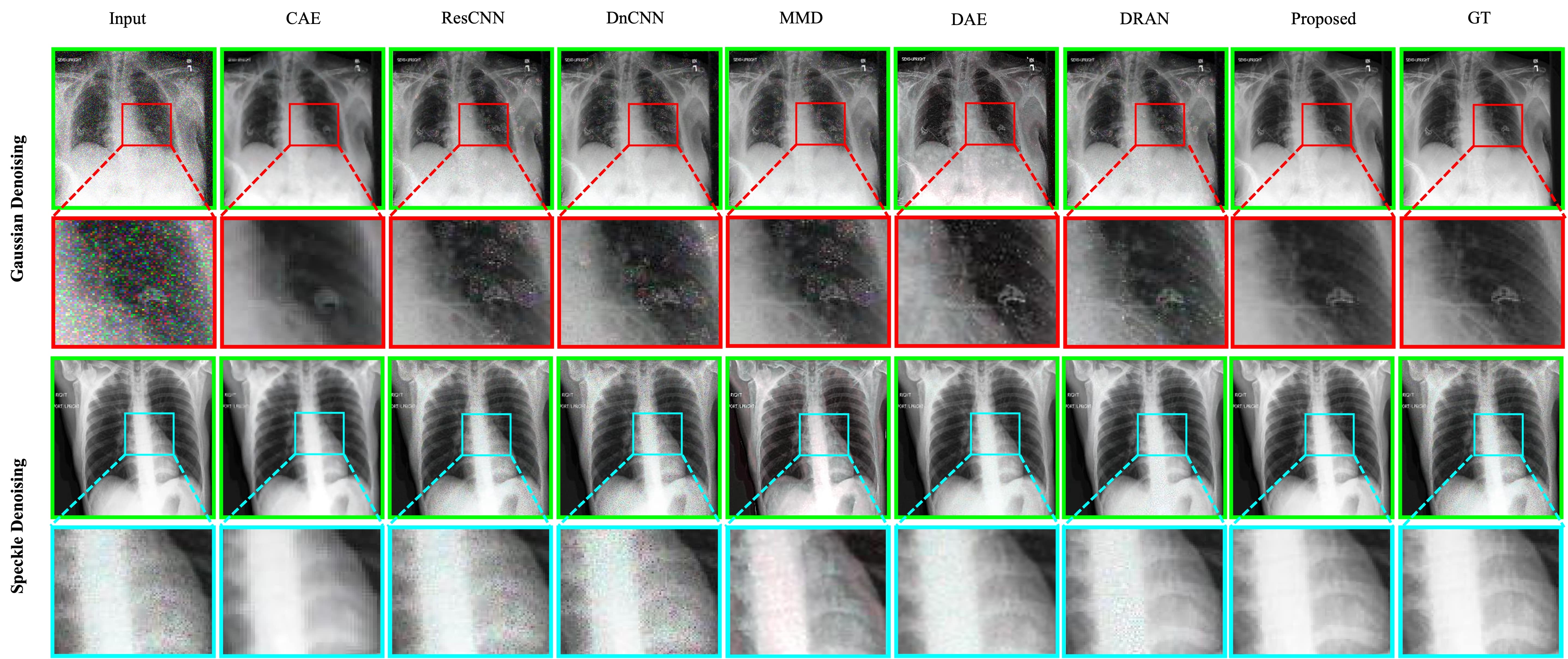
Figure 7: Qualitative comparison for X-ray denoising. The proposed method illustrates consistency in X-ray images as well. The top example shows Gaussian denoising; the bottom depicts speckle denoising. In each row, Left to right: Noisy input, CAE [12], ResCNN [20], DnCNN [26], MMD [6], DAE [13], DRAN [1] [1], proposed method, and ground truth image.

Model	$\sigma$	Gaussian					Speckle					Average
		PSNR	SSIM	$\Delta E$	VIFP	MSE	PSNR	SSIM	$\Delta E$	VIFP	MSE	PSNR	SSIM	$\Delta E$	VIFP	MSE
CAE	10	30.43	0.9178	2.16	0.5049	61.45	30.25	0.9181	2.34	0.5061	63.86	30.34	0.9179	2.25	0.5055	62.65
ResCNN		24.77	0.7455	4.90	0.3551	241.32	24.50	0.7593	4.63	0.4164	247.90	24.64	0.7524	4.77	0.3857	244.61
DnCNN		26.19	0.7812	4.39	0.3879	169.98	24.29	0.7317	4.91	0.3925	259.41	25.24	0.7564	4.65	0.3902	214.69
MMD		23.43	0.8288	7.30	0.4307	331.62	23.43	0.8288	7.30	0.4307	331.62	23.43	0.8288	7.30	0.4307	331.62
DAE		27.63	0.8537	3.47	0.4620	120.63	26.67	0.8264	3.75	0.4796	148.18	27.15	0.8401	3.61	0.4708	134.40
DRAN		33.35	0.9236	2.32	0.5919	34.02	35.11	0.9500	1.47	0.6443	22.60	34.23	0.9368	1.90	0.6181	28.31
Proposed		37.32	0.9687	0.77	0.6798	12.49	37.44	0.9695	0.76	0.6840	12.16	37.38	0.9691	0.77	0.6819	12.32
CAE	25	30.51	0.9150	1.90	0.4965	60.49	30.50	0.9181	1.97	0.5050	60.61	30.50	0.9166	1.94	0.5007	60.55
ResCNN		29.04	0.8603	2.94	0.4578	87.95	26.10	0.8042	3.79	0.4458	176.23	27.57	0.8323	3.36	0.4518	132.09
DnCNN		28.01	0.8299	3.41	0.4190	105.92	25.44	0.7741	4.03	0.4285	197.18	26.73	0.8020	3.72	0.4237	151.55
MMD		23.46	0.8307	7.06	0.4239	327.66	23.46	0.8307	7.06	0.4239	327.66	23.46	0.8307	7.06	0.4239	327.66
DAE		30.28	0.8749	2.71	0.5160	82.47	29.58	0.8777	2.72	0.5422	92.49	29.93	0.8763	2.72	0.5291	87.48
DRAN		30.84	0.8828	2.70	0.5336	60.48	33.18	0.9267	1.79	0.6167	34.88	32.01	0.9047	2.25	0.5751	47.68
Proposed		37.13	0.9677	0.78	0.6740	13.10	37.32	0.9687	0.77	0.6795	12.50	37.22	0.9682	0.78	0.6768	12.80
CAE	50	30.22	0.9071	2.07	0.4763	64.38	30.53	0.9159	1.87	0.4983	60.20	30.38	0.9115	1.97	0.4873	62.29
ResCNN		29.27	0.8781	2.52	0.4892	77.30	29.19	0.8808	2.64	0.5168	86.12	29.23	0.8794	2.58	0.5030	81.71
DnCNN		28.10	0.8335	3.16	0.4175	101.10	26.77	0.8137	3.45	0.4558	148.31	27.44	0.8236	3.31	0.4366	124.70
MMD		23.84	0.8323	6.42	0.4189	303.61	23.84	0.8323	6.42	0.4189	303.61	23.84	0.8323	6.42	0.4189	303.61
DAE		27.94	0.8589	3.22	0.4628	108.87	32.67	0.9199	1.89	0.5910	54.01	30.30	0.8894	2.56	0.5269	81.44
DRAN		26.27	0.7800	3.86	0.4229	169.33	32.53	0.9229	1.75	0.6103	38.33	29.40	0.8515	2.80	0.5166	103.83
Proposed		36.95	0.9671	0.79	0.6708	13.68	37.19	0.9681	0.78	0.6758	12.91	37.07	0.9676	0.79	0.6733	13.29
CAE	75	29.95	0.9000	2.18	0.4598	68.40	30.47	0.9136	1.92	0.4917	61.02	30.21	0.9068	2.05	0.4757	64.71
ResCNN		27.05	0.8392	3.50	0.4299	129.19	30.37	0.9001	2.41	0.5326	63.78	28.71	0.8697	2.95	0.4812	96.49
DnCNN		26.53	0.8146	3.76	0.4050	144.71	27.71	0.8367	3.16	0.4732	119.59	27.12	0.8256	3.46	0.4391	132.15
MMD		23.82	0.8275	6.14	0.4116	305.46	23.82	0.8275	6.14	0.4116	305.46	23.82	0.8275	6.14	0.4116	305.46
DAE		26.09	0.8039	3.82	0.3846	160.53	33.01	0.9223	1.97	0.5861	50.58	29.55	0.8631	2.89	0.4853	105.56
DRAN		23.89	0.6918	5.35	0.3270	270.18	30.86	0.8978	1.97	0.5786	54.85	27.38	0.7948	3.66	0.4528	162.52
Proposed		36.79	0.9667	0.80	0.6688	14.19	37.09	0.9677	0.78	0.6737	13.22	36.94	0.9672	0.79	0.6713	13.70

TABLE II: Quantative comparison for X-ray denoising. The proposed method outperforms existing denoising methods by a notable margin.

III-A3 CT Images

CT scan is a type of medical imaging that uses X-rays and computer processing to create detailed information [50]. To further confirm the performance of the proposed method in radiology images. Table. III, illustrates the quantitative comparison on CT images. The proposed method shows consistency in CT denoising and achieved a performance gain of over 4.34 in PSNR, 0.0442 in SSIM, 0.97 in $\Delta E$, 0.0658 in VIFP, and 24.97 in MSE metric for speckle denoising. Similarly, it outperforms the existing denoising methods by 8.46 in PSNR, 0.1480 in SSIM, 2.77 in $\Delta E$, 0.2045 in VIFP, and 120.14 in MSE metric for Gaussian denoising.

Fig. 8 illustrates the visual comparison between the denoising methods. The proposed method can plausibly denoise the CT images as well. It can reduce noises from the CT images without illustrating any visual artifacts.

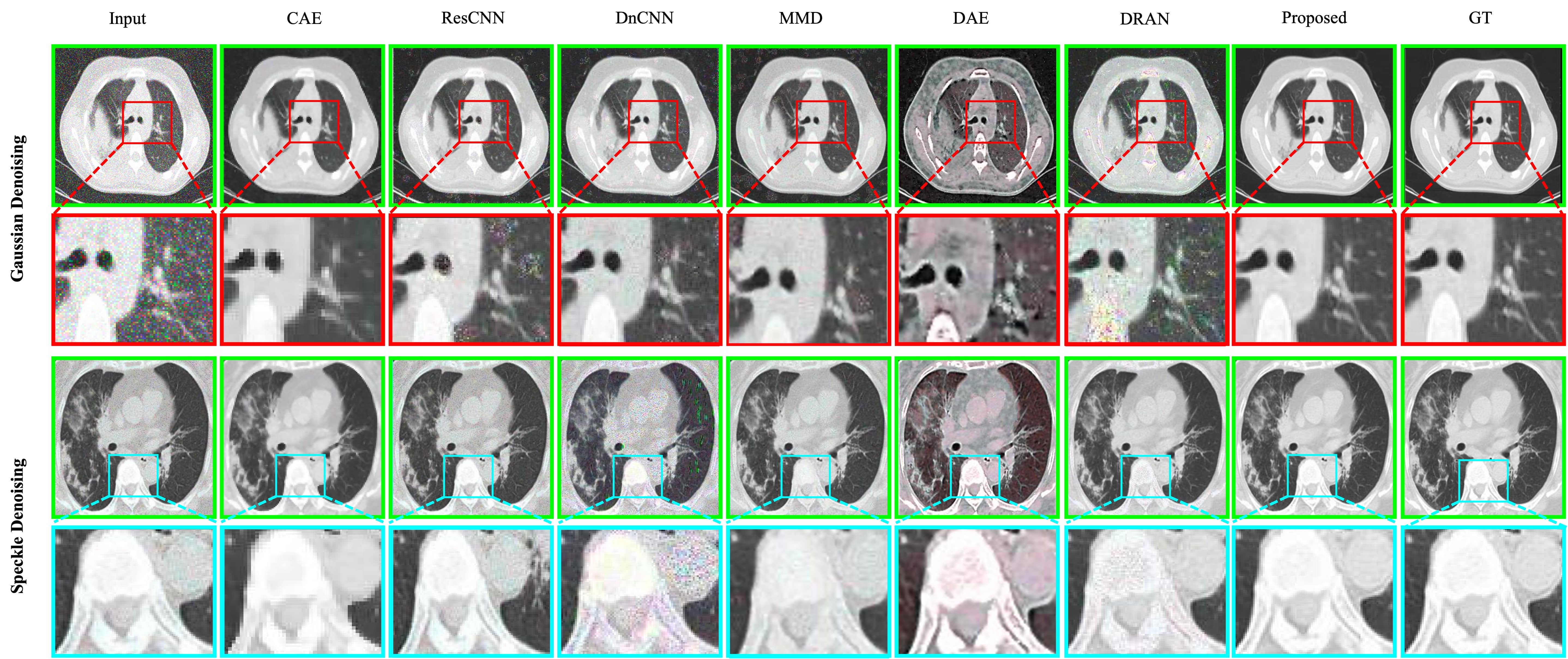
Figure 8: Qualitative comparison for CT denoising. The proposed method produces visually plausible images compared to the existing denoising methods. The top example depicts Gaussian denoising; the bottom illustrates speckle denoising. In each row, Left to right: Noisy input, CAE [12], ResCNN [20], DnCNN [26], MMD [6], DAE [13], DRAN [1] [1], proposed method, and ground truth image.

Model	$\sigma$	Gaussian					Speckle					Average
		PSNR	SSIM	$\Delta E$	VIFP	MSE	PSNR	SSIM	$\Delta E$	VIFP	MSE	PSNR	SSIM	$\Delta E$	VIFP	MSE
CAE	10	27.39	0.8882	2.39	0.4311	138.61	27.30	0.8886	2.49	0.4316	141.21	27.34	0.8884	2.44	0.4314	139.91
ResCNN		23.92	0.7214	7.43	0.3771	286.38	22.89	0.7051	7.67	0.3745	358.90	23.41	0.7133	7.55	0.3758	322.64
DnCNN		23.29	0.6763	8.02	0.3465	347.46	22.28	0.6604	8.09	0.3452	427.39	22.79	0.6684	8.05	0.3459	387.43
MMD		18.60	0.8004	9.89	0.4403	1135.39	18.60	0.8004	9.89	0.4403	1135.39	18.60	0.8004	9.89	0.4403	1135.39
DAE		25.05	0.7498	6.89	0.4074	238.80	24.38	0.7460	6.95	0.4130	268.49	24.72	0.7479	6.92	0.4102	253.65
DRAN		36.72	0.9624	1.64	0.7226	17.48	37.54	0.9699	1.39	0.7554	14.31	37.13	0.9662	1.52	0.7390	15.90
Proposed		42.20	0.9869	0.59	0.8303	5.64	42.93	0.9880	0.54	0.8471	5.15	42.56	0.9875	0.57	0.8387	5.40
CAE	25	27.42	0.8853	2.26	0.4259	138.14	27.41	0.8883	2.28	0.4311	138.42	27.42	0.8868	2.27	0.4285	138.28
ResCNN		26.50	0.8010	5.71	0.4435	167.40	24.34	0.7540	6.69	0.4076	270.43	25.42	0.7775	6.20	0.4256	218.92
DnCNN		25.22	0.7448	6.84	0.3907	224.91	23.36	0.7092	7.35	0.3767	333.93	24.29	0.7270	7.10	0.3837	279.42
MMD		18.80	0.8014	9.63	0.4337	1099.53	18.80	0.8014	9.63	0.4337	1099.53	18.80	0.8014	9.63	0.4337	1099.53
DAE		26.84	0.7929	5.70	0.4494	174.33	25.20	0.7718	6.37	0.4324	243.72	26.02	0.7823	6.04	0.4409	209.03
DRAN		32.01	0.8950	3.13	0.5758	62.51	35.50	0.9500	1.85	0.6961	24.13	33.76	0.9225	2.49	0.6360	43.32
Proposed		40.99	0.9847	0.64	0.8027	6.96	42.02	0.9864	0.58	0.8253	5.83	41.51	0.9856	0.61	0.8140	6.40
CAE	50	27.27	0.8778	2.35	0.4136	142.23	27.43	0.8862	2.24	0.4264	138.15	27.35	0.8820	2.29	0.4200	140.19
ResCNN		27.65	0.8506	4.23	0.4986	116.56	25.83	0.7992	5.84	0.4427	195.83	26.74	0.8249	5.03	0.4707	156.20
DnCNN		26.55	0.8134	5.29	0.4509	155.26	25.07	0.7691	6.39	0.4181	227.94	25.81	0.7913	5.84	0.4345	191.60
MMD		18.97	0.7974	9.40	0.4209	1069.68	18.97	0.7974	9.40	0.4209	1069.68	18.97	0.7974	9.40	0.4209	1069.68
DAE		25.67	0.7745	5.91	0.4354	250.16	26.03	0.7916	6.07	0.4491	228.54	25.85	0.7830	5.99	0.4423	239.35
DRAN		27.94	0.8229	4.84	0.4468	130.15	33.23	0.9203	2.51	0.6217	40.11	30.59	0.8716	3.68	0.5343	85.13
Proposed		40.06	0.983	0.69	0.7848	8.47	41.12	0.9850	0.62	0.8057	6.79	40.59	0.9840	0.66	0.7953	7.63
CAE	75	27.09	0.8709	2.43	0.4036	147.23	27.40	0.8842	2.26	0.4222	138.77	27.25	0.8776	2.34	0.4129	143.00
ResCNN		26.57	0.8261	4.98	0.4677	158.42	27.30	0.8390	5.11	0.4792	144.05	26.94	0.8326	5.05	0.4735	151.24
DnCNN		25.61	0.8176	5.31	0.4586	188.14	26.54	0.8112	5.61	0.4538	166.93	26.08	0.8144	5.46	0.4562	177.53
MMD		18.97	0.7894	9.37	0.4084	1071.27	18.97	0.7894	9.37	0.4084	1071.27	18.97	0.7894	9.37	0.4084	1071.27
DAE		25.21	0.7915	5.60	0.4289	260.84	26.76	0.8047	5.81	0.4645	219.53	25.98	0.7981	5.71	0.4467	240.18
DRAN		27.32	0.8158	4.98	0.4313	141.79	31.66	0.8949	3.08	0.5686	59.29	29.49	0.8554	4.03	0.5000	100.54
Proposed		39.50	0.9819	0.74	0.7752	9.58	40.55	0.9842	0.64	0.7949	7.60	40.03	0.9831	0.69	0.7851	8.59

TABLE III: Quantative comparison for CT denoising. The proposed method demonstrates consistency in CT denoising as well.

III-A4 Skin Images

Skin lesion images are medical images that show various skin abnormalities, including moles, freckles, rashes, and tumors. Such medical image types are contaminated with numerous noise patterns. This study extensively evaluated our proposed two-stage network for multi-pattern denoising. Table. IV illustrates the quantitative comparison for Gaussian and speckle denoising. The proposed method achieved significant improvement in skin image denoising. The proposed method depicts an improvement for speckle denoising by improving 8.51 in PSNR, 0.1184 in SSIM, 1.34 in $\Delta E$, 0.2214 in VIFP, and 28.20 in MSE score. The proposed method also illustrates a performance gain of 10.68 in PSNR, 0.1868 in SSIM, 2.20 in $\Delta E$, 0.3005 in VIFP, and 59.33 in MSE for Gaussian denoising.

In addition to the quantitative comparison, we extensively evaluated the deep models with visual results, as shown in Fig. 9. It is visible that the proposed method can produce clean medical images without any visually disturbing artifacts for speckle and Gaussian denoising.

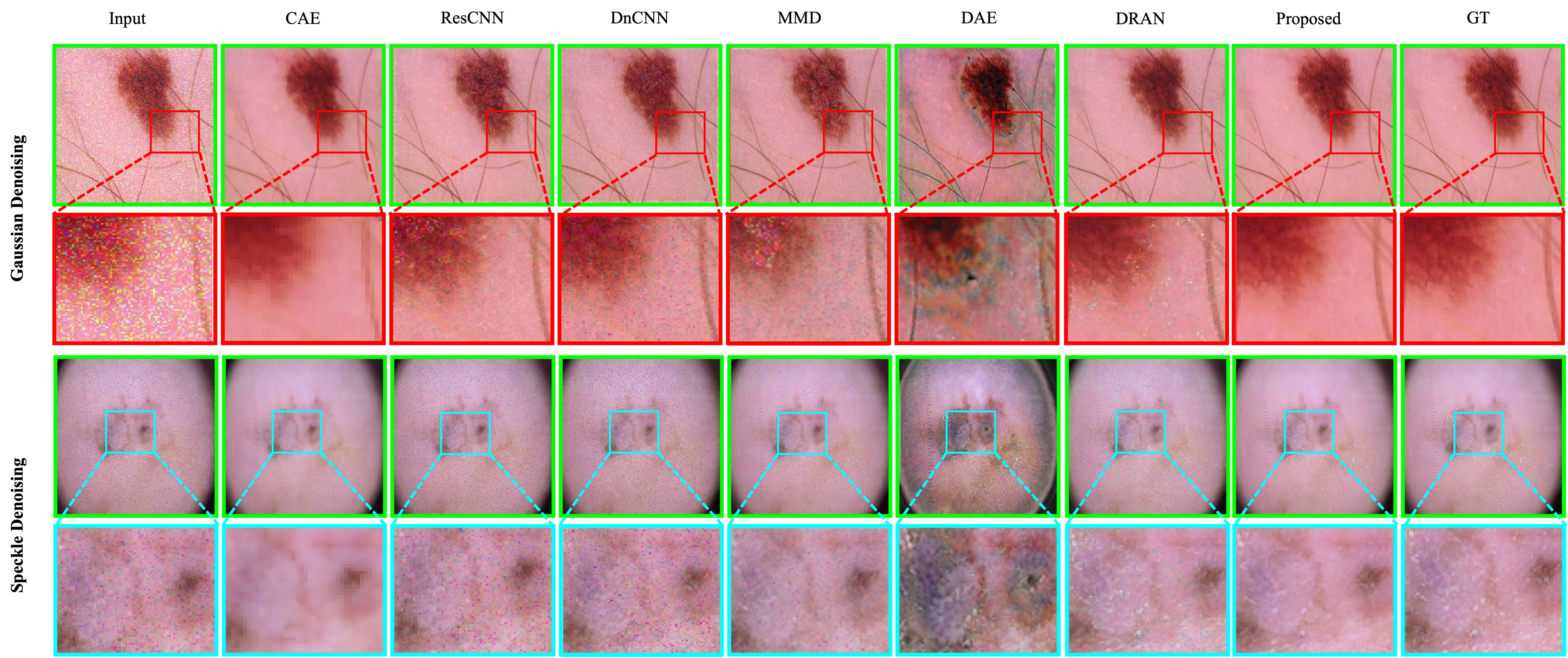
Figure 9: Qualitative comparison for skin image denoising. The proposed method outperforms the existing denoising methods by generating plausible images. The top example illustrates Gaussian denoising; the bottom demonstrates speckle denoising. In each row, Left to right: Noisy input, CAE [12], ResCNN [20], DnCNN [26], MMD [6], DAE [13], DRAN [1] [1], proposed method, and ground truth image.

Model	$\sigma$	Gaussian					Speckle					Average
		PSNR	SSIM	$\Delta E$	VIFP	MSE	PSNR	SSIM	$\Delta E$	VIFP	MSE	PSNR	SSIM	$\Delta E$	VIFP	MSE
CAE	10	34.84	0.9209	1.84	0.4493	25.22	34.57	0.9220	1.88	0.4533	26.64	34.70	0.9214	1.86	0.4513	25.93
ResCNN		21.41	0.3084	9.49	0.1549	503.15	20.59	0.2827	10.57	0.1499	599.68	21.00	0.2955	10.03	0.1524	551.41
DnCNN		20.53	0.2655	10.61	0.1464	603.55	20.17	0.2596	11.01	0.1513	653.57	20.35	0.2626	10.81	0.1488	628.56
MMD		20.41	0.7221	8.61	0.4830	678.19	20.41	0.7221	8.61	0.4830	678.19	20.41	0.7221	8.61	0.4830	678.19
DAE		22.26	0.3819	8.98	0.1885	447.88	22.15	0.3810	9.11	0.1969	439.06	22.21	0.3814	9.04	0.1927	443.47
DRAN		37.35	0.9350	1.54	0.6006	13.41	38.48	0.9488	1.35	0.6587	10.75	37.92	0.9419	1.45	0.6296	12.08
Proposed		42.64	0.9788	0.89	0.7393	3.97	43.43	0.9814	0.84	0.7649	3.29	43.04	0.9801	0.87	0.7521	3.63
CAE	25	34.84	0.9151	1.84	0.4312	24.94	34.92	0.9198	1.81	0.4472	24.77	34.88	0.9174	1.83	0.4392	24.85
ResCNN		24.04	0.4300	7.02	0.1941	314.55	22.40	0.3600	8.45	0.1840	420.60	23.22	0.3950	7.73	0.1890	367.58
DnCNN		22.37	0.3358	8.51	0.1625	385.6	20.93	0.2998	9.83	0.1658	542.33	21.65	0.3178	9.17	0.1641	463.96
MMD		20.15	0.7071	8.88	0.4394	732.22	20.15	0.7071	8.88	0.4394	732.22	20.15	0.7071	8.88	0.4394	732.22
DAE		24.96	0.5147	6.63	0.2391	341.52	22.91	0.4192	8.31	0.2123	419.90	23.94	0.4669	7.47	0.2257	380.71
DRAN		33.85	0.8663	2.20	0.4802	28.46	36.46	0.9144	1.67	0.5739	16.24	35.15	0.8903	1.94	0.5270	22.35
Proposed		42.61	0.9776	0.89	0.7306	4.11	43.1	0.9790	0.86	0.7416	3.58	42.85	0.9783	0.87	0.7361	3.84
CAE	50	34.19	0.904	1.99	0.3993	28.07	34.73	0.9141	1.84	0.4291	25.34	34.46	0.9090	1.91	0.4142	26.71
ResCNN		25.60	0.6005	5.42	0.2613	224.78	25.00	0.4871	6.33	0.2283	263.92	25.30	0.5438	5.87	0.2448	244.35
DnCNN		25.84	0.5778	5.20	0.2454	176.86	23.25	0.3983	7.47	0.1979	316.48	24.55	0.4880	6.34	0.2216	246.67
MMD		19.62	0.6885	9.54	0.3886	837.40	19.62	0.6885	9.54	0.3886	837.40	19.62	0.6885	9.54	0.3886	837.40
DAE		25.54	0.5740	5.04	0.2359	194.36	26.61	0.5778	5.55	0.2775	259.65	26.08	0.5759	5.30	0.2567	227.01
DRAN		29.23	0.7201	3.73	0.3513	80.50	32.84	0.8292	2.46	0.4641	36.32	31.04	0.7747	3.10	0.4077	58.41
Proposed		42.56	0.9775	0.89	0.7315	4.23	42.9	0.9783	0.87	0.7358	3.82	42.73	0.9779	0.88	0.7337	4.02
CAE	75	33.87	0.8941	2.09	0.3748	29.94	34.46	0.9084	1.90	0.4123	26.52	34.17	0.9012	2.00	0.3936	28.23
ResCNN		23.45	0.5201	7.70	0.2183	312.98	27.20	0.6096	4.92	0.2784	179.16	25.32	0.5649	6.31	0.2484	246.07
DnCNN		24.41	0.5516	6.72	0.2175	240.72	25.55	0.5200	5.60	0.2401	190.39	24.98	0.5358	6.16	0.2288	215.56
MMD		19.15	0.6732	10.12	0.3546	929.46	19.15	0.6732	10.12	0.3546	929.46	19.15	0.6732	10.12	0.3546	929.46
DAE		24.37	0.5769	6.06	0.2194	240.96	27.77	0.6263	4.31	0.2884	130.90	26.07	0.6016	5.19	0.2539	185.93
DRAN		27.08	0.6423	4.89	0.2964	131.62	30.37	0.7506	3.33	0.3947	64.16	28.72	0.6964	4.11	0.3456	97.89
Proposed		42.40	0.9771	0.90	0.7292	4.38	42.77	0.9780	0.88	0.7346	3.98	42.59	0.9775	0.89	0.7319	4.18

TABLE IV: Quantitative comparison for skin image denoising. The proposed method can equally denoise the skin images.

III-A5 Microscopy Images

Microscopy plays a crucial role in medical imaging as it allows researchers and medical professionals to study the structure and function of cells, tissues, and organs in the human body at a microscopic level. Despite having a substantial impact, these also can be affected by numerous noise patterns. Table. V illustrates the quantitative comparison for the microscopic images. The proposed method can improve the cumulative performance of 5.79 in PSNR, 0.1184 in SSIM, 0.24 in $\Delta E$, 0.1045 in VIFP, and 11.825 in MSE metric for speckle denoising. It also illustrates a performance gain of 6.59 in PSNR, 0.0805 in SSIM, 0.87 in $\Delta E$, 0.1742 in VIFP, and 25.03 in MSE metric for Gaussian denoising.

Similar to radiology and skin images, the proposed method illustrates significant performance gain over the existing denoising methods for microscopic images. Fig. 10 further confirms the performance gain of the proposed method by qualitative results. Overall, the proposed method illustrates consistent all comparing modalities in qualitative and quantitative comparisons.

- -

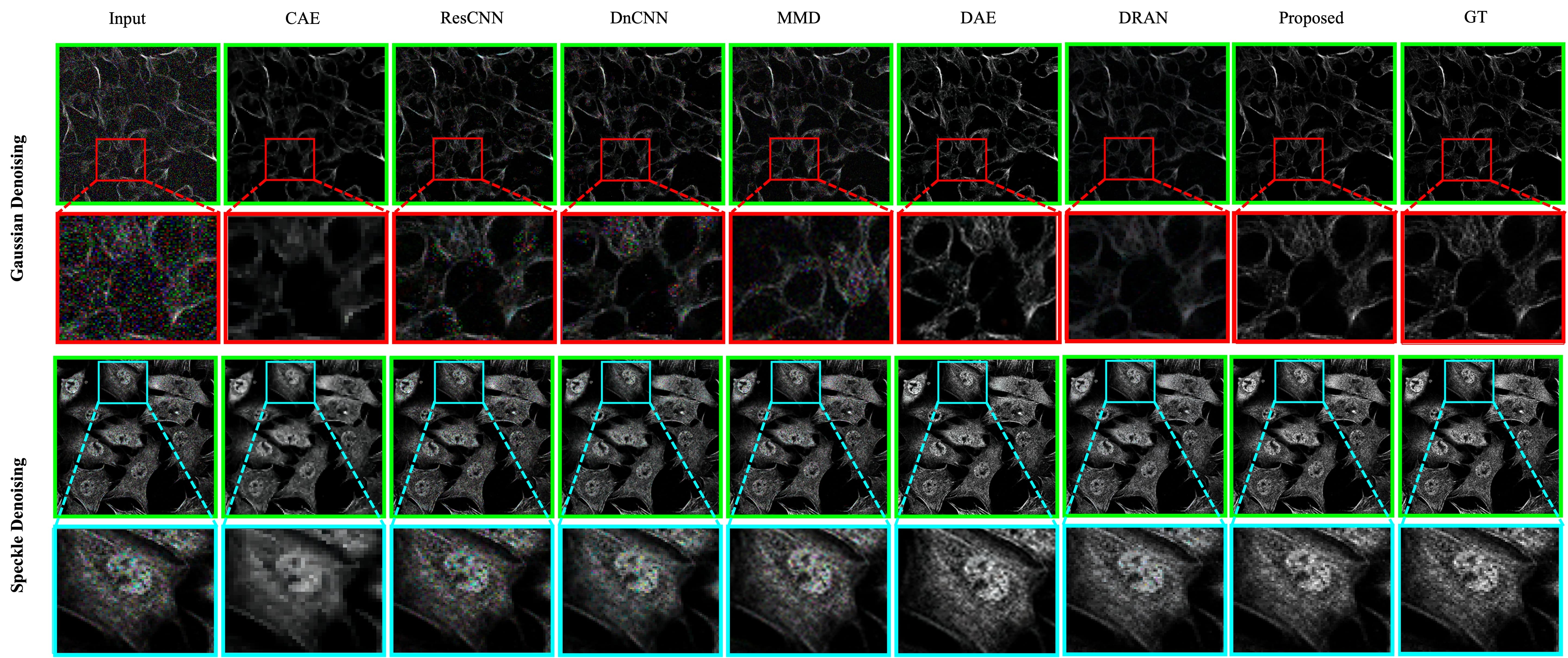
Figure 10: Qualitative comparison for microscopy image denoising. The proposed method generates visually plausible images without illustrating visual artifacts. The top example illustrates Gaussian denoising; the bottom illustrates speckle denoising. In each row, Left to right: Noisy input, CAE [12], ResCNN [20], DnCNN [26], MMD [6], DAE [13], DRAN [1] [1], proposed method, and ground truth image.

Model	$\sigma$	Gaussian					Speckle					Average
		PSNR	SSIM	$\Delta E$	VIFP	MSE	PSNR	SSIM	$\Delta E$	VIFP	MSE	PSNR	SSIM	$\Delta E$	VIFP	MSE
CAE	10	32.07	0.9094	0.98	0.3726	79.23	32.01	0.9087	0.97	0.3730	80.68	32.04	0.9091	0.98	0.3728	79.96
ResCNN		30.64	0.8710	2.44	0.3163	83.31	28.10	0.8294	2.68	0.2272	175.00	29.37	0.8502	2.56	0.2718	129.15
DnCNN		30.34	0.8660	2.43	0.3216	90.11	28.11	0.8132	2.43	0.2432	158.22	29.23	0.8396	2.43	0.2824	124.17
MMD		26.78	0.7327	3.16	0.5058	385.58	26.78	0.7327	3.16	0.5058	385.58	26.78	0.7327	3.16	0.5058	385.58
DAE		29.55	0.8514	2.80	0.2996	108.10	27.22	0.8262	2.76	0.2225	174.56	28.39	0.8388	2.78	0.2610	141.33
DRAN		37.11	0.9693	0.67	0.5904	19.09	38.63	0.9859	0.46	0.6900	15.12	37.87	0.9776	0.56	0.6402	17.11
Proposed		43.14	0.9888	0.29	0.7415	5.74	44.35	0.9927	0.25	0.7848	4.93	43.74	0.9908	0.27	0.7632	5.34
CAE	25	31.95	0.9053	0.99	0.3640	80.12	32.05	0.9096	0.97	0.3749	79.69	32.00	0.9075	0.98	0.3695	79.91
ResCNN		30.63	0.8449	2.57	0.3548	65.50	28.33	0.8356	2.65	0.2340	163.00	29.48	0.8403	2.61	0.2944	114.25
DnCNN		29.95	0.8541	2.70	0.3361	79.96	28.38	0.8236	2.47	0.2573	148.05	29.16	0.8389	2.59	0.2967	114.01
MMD		26.62	0.7290	3.20	0.5015	388.86	26.62	0.7290	3.20	0.5015	388.86	26.62	0.7290	3.20	0.5015	388.86
DAE		31.14	0.8759	2.49	0.3877	58.51	27.39	0.8345	2.71	0.2315	165.22	29.27	0.8552	2.60	0.3096	111.87
DRAN		34.91	0.9408	0.98	0.5186	29.30	38.36	0.9852	0.48	0.6823	16.01	36.63	0.9630	0.73	0.6005	22.66
Proposed		41.33	0.9832	0.34	0.6899	8.20	44.19	0.9926	0.26	0.7825	5.06	42.76	0.9879	0.30	0.7362	6.63
CAE	50	31.73	0.8993	1.02	0.3514	82.96	32.08	0.9103	0.97	0.3763	79.29	31.9	0.9048	0.99	0.3639	81.13
ResCNN		27.06	0.6417	4.36	0.3332	129.69	28.67	0.8453	2.59	0.2451	144.51	27.87	0.7435	3.48	0.2892	137.10
DnCNN		27.2	0.7543	3.29	0.3370	126.55	28.65	0.8384	2.46	0.2708	131.70	27.93	0.7964	2.87	0.3039	129.13
MMD		26.23	0.7200	3.29	0.4849	404.30	26.23	0.7200	3.29	0.4849	404.30	26.23	0.7200	3.29	0.4849	404.30
DAE		26.80	0.6347	4.70	0.3271	140.48	27.42	0.8384	2.66	0.2371	161.80	27.11	0.7365	3.68	0.2821	151.14
DRAN		33.00	0.8785	1.47	0.4692	41.63	37.85	0.9836	0.52	0.6672	17.98	35.42	0.9311	1.00	0.5682	29.80
Proposed		39.74	0.9781	0.41	0.6500	12.17	43.69	0.9923	0.27	0.7750	5.54	41.71	0.9852	0.34	0.7125	8.86
CAE	75	31.52	0.8938	1.06	0.3397	86.04	32.08	0.9105	0.97	0.3767	79.44	31.8	0.9022	1.01	0.3582	82.74
ResCNN		20.7	0.2860	12.03	0.2087	558.26	28.89	0.8526	2.54	0.2528	131.27	24.8	0.5693	7.29	0.2308	344.76
DnCNN		21.28	0.3096	10.82	0.2189	487.45	28.87	0.8486	2.44	0.2812	122.6	25.07	0.5791	6.63	0.2501	305.02
MMD		26.05	0.7165	3.34	0.4733	412.95	26.05	0.7165	3.34	0.4733	412.95	26.05	0.7165	3.34	0.4733	412.95
DAE		21.29	0.3065	11.01	0.2202	486.13	27.40	0.8447	2.61	0.2427	157.53	24.35	0.5756	6.81	0.2314	321.83
DRAN		31.75	0.8151	1.85	0.4365	51.21	37.31	0.9816	0.56	0.6492	20.00	34.53	0.8984	1.21	0.5429	35.60
Proposed		38.91	0.9754	0.46	0.6302	15.02	43.09	0.9918	0.28	0.7651	6.28	41.00	0.9836	0.37	0.6977	10.65

TABLE V: Quantitative comparison for microscopic image denoising. The proposed method outperforms existing methods on microscopic images as well.

III-B Real-world Medical Image Denoising

Apart from the synthesized noisy images, we evaluated our method with real-world noisy CT images [51]. Therefore, the model is tuned to real-world noisy medical images. The proposed method has retrained leveraging transfer learning with low-dose sharp kernel CT images [3]. The trained model was evaluated with noisy CT images reconstructed with soft and sharp kernels, as shown in Fig. 11.

The visual results clarify that the proposed method can handle real-world noisy medical images. The proposed method can substantially reduce the low-dose CT noises without showing visual artifacts. In complex spatial regions, it also maintains salient information intact. Overall, the proposed method generates cleaner images and ensures plausible perceptual quality.

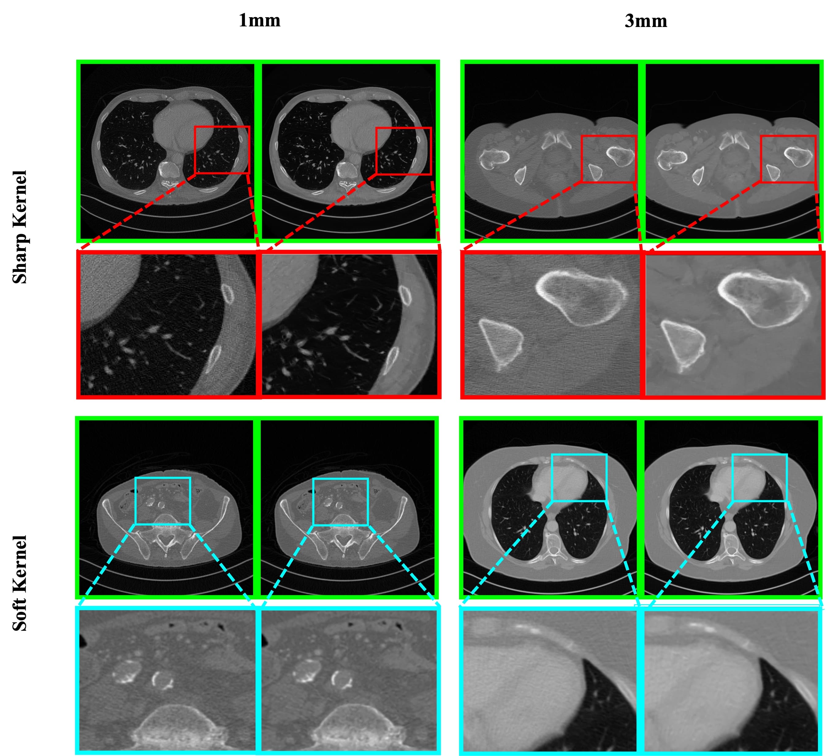
Figure 11: Real-world low-dose CT image denoising with the proposed method. The proposed method can remove real-world noise without losing salient information. In each pair, left: low-dose noisy CT image and right: denoised image.

III-C Ablation Study

The efficiency of the proposed components has been confirmed with relevant ablation experiments. We evaluated the proposed components with objective and subjective evaluation, similar to the state-of-the-art comparisons. For better readability, we combined all image modalities into a unified dataset. The evaluation metrics, noise levels, and noise patterns remain unchanged. Table. VI illustrates the feasibility of the proposed network components. NEN denotes a Noise estimation network (stage I) and TWN denotes the proposed two-stage network without NOB.

It is noticeable that the proposed two-stage denoising strategy with self-guided noise attention allows us to achieve state-of-the-art performance for Gaussian and speckle denoising. Fig. 12 also confirms the efficiency of the proposed method in denoising.

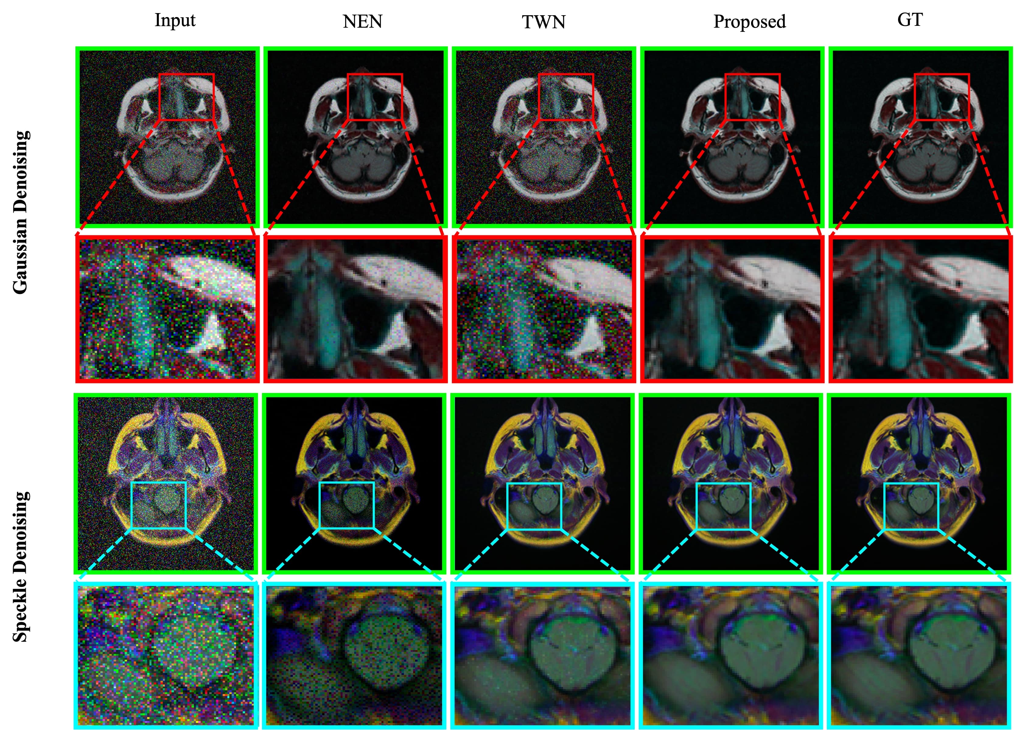
Figure 12: Qualitative evaluation of the proposed method. The top example depicts Gaussian denoising; the bottom illustrates speckle denoising. In each row, Left to right: Noisy Input, the result obtained by NEN (stage I), TWN (two-stage network without NOB), Proposed (two-stage network with NOB), and ground-truth image. It can be seen that the proposed two-stage learning strategy and noise attention help to produce clean images without showing artifacts.

Model	$\sigma$	Gaussian					Speckle					Average
		PSNR	SSIM	$\Delta E$	VIFP	MSE	PSNR	SSIM	$\Delta E$	VIFP	MSE	PSNR	SSIM	$\Delta E$	VIFP	MSE
NEN	10	36.84	0.9508	1.51	0.6572	22.87	36.26	0.9398	1.56	0.6421	18.83	36.55	0.9453	1.54	0.6497	20.85
TWN		34.38	0.8690	2.47	0.5605	26.18	39.38	0.9749	0.94	0.7338	11.18	36.88	0.9220	1.70	0.6471	18.68
Proposed		41.51	0.9811	0.69	0.7374	6.57	43.58	0.9853	0.54	0.7936	5.50	42.54	0.9832	0.61	0.7655	6.04
Stage-I	25	36.71	0.9454	1.47	0.6437	23.58	33.68	0.8999	2.21	0.5623	40.36	35.19	0.9226	1.84	0.6030	31.97
WNN		31.64	0.7892	3.60	0.4842	61.63	39.92	0.9752	0.93	0.7337	10.29	35.78	0.8822	2.27	0.6089	35.96
Proposed		41.08	0.9799	0.71	0.7250	7.17	43.03	0.9846	0.56	0.7841	5.73	42.05	0.9823	0.63	0.7546	6.45
Stage-I	50	35.26	0.9153	1.77	0.6072	41.72	31.07	0.8315	3.21	0.4807	102.14	33.16	0.8734	2.49	0.5440	71.93
TWN		28.88	0.7034	5.03	0.4189	155.72	39.57	0.9731	1.00	0.7203	11.08	34.22	0.8382	3.01	0.5696	83.40
Proposed		40.71	0.9789	0.73	0.7160	7.84	42.59	0.9840	0.59	0.7754	6.03	41.65	0.9814	0.66	0.7457	6.94
Stage-I	75	33.85	0.8819	2.22	0.5676	69.43	29.25	0.7796	4.02	0.4262	172.64	31.55	0.8308	3.12	0.4969	121.04
TWN		26.86	0.6430	6.27	0.3747	277.65	38.74	0.9656	1.18	0.6961	14.27	32.80	0.8043	3.72	0.5354	145.96
Proposed		40.42	0.9780	0.74	0.7092	8.44	42.25	0.9835	0.61	0.7684	6.34	41.33	0.9807	0.68	0.7388	7.39

TABLE VI: Quantitative evaluation of the proposed two-stage method. The novel components help to achieve state-of-the-art performance for multi-modal medical image denoising.

In addition to the ablation experiments, we visualized the validation performance of the proposed network over the training period. Fig. 13 illustrates the validation performance of the proposed method and its variants for speckle and Gaussian denoising. It is perceptible that the proposed components help the proposed method with two-stage denoising and noise attention help to achieve a stable training result with improved denoising performance in all evaluation metrics.

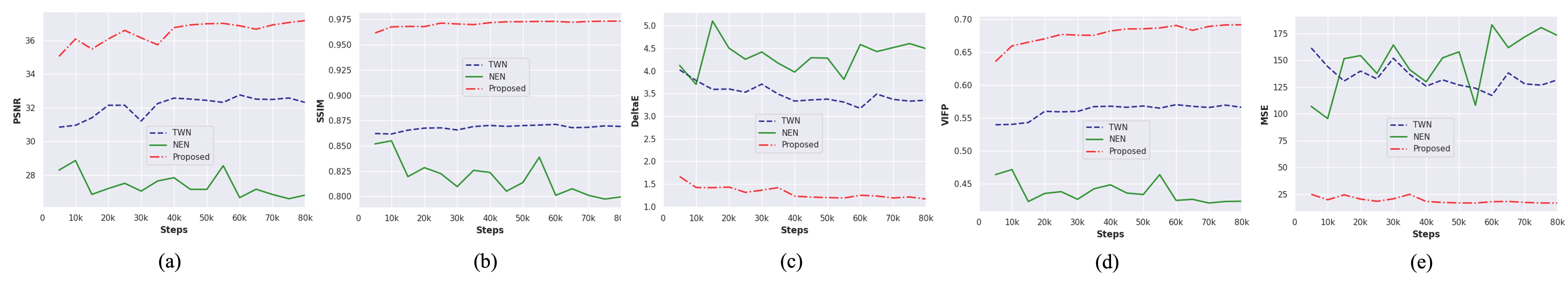
Figure 13: Validation results of the proposed method and its variants. (a) PSNR vs. steps. (b) SSIM vs. steps. (C) $\Delta E$ vs. steps. (d) VIFP vs. steps. (e) MSE vs. steps.

III-D Inference Analysis

Despite showing a significant performance gain over state-of-the-art denoising methods, the proposed two-stage denoising method is computationally efficient. Table. VII illustrates the proposed method comprises only 586,242 trainable parameters with 38.34 G Macs operations. In our setup, it takes only 25.73 ms to denoise an input image with $256\times 256\times 3$ pixels. Overall, it reveals the feasibility of the proposed method for real-world lightweight applications [52, 53].

Model	NEN	RN	Two-stage
Trainable Parameters	283,776	302,466	586,242
MAC(G)	18.56	19.78	38.34
Memory Consumption (MB)	835.33	900.90	1,736
Inference Time (ms)	9.96	15.77	25.73

TABLE VII: Trainable parameters and inference time of the proposed method. Despite showing significant performance gain, the proposed method is also computationally lightweight.

III-E Discussion

A generic method for denoising in medical imaging offers several advantages. This simplified approach can effectively utilize cross-modal domain knowledge to enhance denoising performance. This study incorporates a novel noise simulation method based on real-world scenarios. However, in extreme cases, the proposed method can illustrate shortcomings due to the lack of real-world data samples. The limitation of the proposed method indicates the future directions for multi-modal medical image-denoising. A real-world dataset could help future studies develop a robust real-world generic denoising solution. The modal learning ability of the proposed method also discloses the possibility of learning medical image denoising by leveraging federated learning. It could allow the process of learning denoising in a decentralized manner to reduce data dependency.

IV Conclusion

This study proposed a two-stage deep denoising method for learning multi-pattern noise from multi-modal medical images. The proposed network estimates the residual noise in Stage I and utilizes it in a later stage for refining denoising output by leveraging a novel noise attention mechanism. Such a learning strategy allowed the proposed method to achieve state-of-the-art performance on Gaussian and speckle denoising in numerous medical modalities. In a qualitative comparison, the proposed two-stage network outperforms existing denoising methods and illustrated a performance gain of 7.64 in PSNR, 0.1021 in SSIM, 0.80 in $\Delta E$, 0.1855 in VIFP, and 18.54 in MSE metrics. There are plans to collect a real-world noisy medical dataset to study the proposed method in the foreseeable future.

References

- [1] S. Sharif, R. A. Naqvi, and M. Biswas, “Learning medical image denoising with deep dynamic residual attention network,” Mathematics, vol. 8, no. 12, p. 2192, 2020.
- [2] M. Geng, X. Meng, J. Yu, L. Zhu, L. Jin, Z. Jiang, B. Qiu, H. Li, H. Kong, J. Yuan et al., “Content-noise complementary learning for medical image denoising,” IEEE Transactions on Medical Imaging, vol. 41, no. 2, pp. 407–419, 2021.
- [3] Y. Lei, C. Niu, J. Zhang, G. Wang, and H. Shan, “Ct image denoising and deblurring with deep learning: Current status and perspectives,” IEEE Transactions on Radiation and Plasma Medical Sciences, 2023.
- [4] G. Lee and H. Fujita, Deep learning in medical image analysis: challenges and applications. Springer, 2020, vol. 1213.
- [5] K. S. H. Kulathilake, N. A. Abdullah, A. Q. M. Sabri, A. R. Bandara, and K. W. Lai, “A review on self-adaptation approaches and techniques in medical image denoising algorithms,” Multimedia Tools and Applications, vol. 81, no. 26, pp. 37 591–37 626, 2022.
- [6] W. El-Shafai, A. Mahmoud, A. Ali, E. El-Rabaie, T. Taha, O. Zahran, A. El-Fishawy, N. Soliman, A. Alhussan, and F. Abd El-Samie, “Deep cnn model for multimodal medical image denoising,” Comput. Mater. Contin, vol. 73, pp. 3795–3814, 2022.
- [7] J. Wang, Y. Guo, Y. Ying, Y. Liu, and Q. Peng, “Fast non-local algorithm for image denoising,” in 2006 International Conference on Image Processing. IEEE, 2006, pp. 1429–1432.
- [8] M. Elad and M. Aharon, “Image denoising via sparse and redundant representations over learned dictionaries,” IEEE Transactions on Image processing, vol. 15, no. 12, pp. 3736–3745, 2006.
- [9] A. S. Arif, S. Mansor, and R. Logeswaran, “Combined bilateral and anisotropic-diffusion filters for medical image de-noising,” in 2011 IEEE Student Conference on Research and Development. IEEE, 2011, pp. 420–424.
- [10] D. Bhonsle, V. Chandra, and G. Sinha, “Medical image denoising using bilateral filter,” International Journal of Image, Graphics and Signal Processing, vol. 4, no. 6, p. 36, 2012.
- [11] K. Dabov, A. Foi, V. Katkovnik, and K. Egiazarian, “Image denoising by sparse 3-d transform-domain collaborative filtering,” IEEE Transactions on image processing, vol. 16, no. 8, pp. 2080–2095, 2007.
- [12] L. Gondara, “Medical image denoising using convolutional denoising autoencoders,” in 2016 IEEE 16th International Conference on Data Mining Workshops (ICDMW). IEEE, 2016, pp. 241–246.
- [13] W. El-Shafai, S. A. El-Nabi, E.-S. M. El-Rabaie, A. M. Ali, N. F. Soliman, A. D. Algarni, A. El-Samie, and E. Fathi, “Efficient deep-learning-based autoencoder denoising approach for medical image diagnosis.” Computers, Materials & Continua, vol. 70, no. 3, 2022.
- [14] H. Chen, Y. Zhang, M. K. Kalra, F. Lin, Y. Chen, P. Liao, J. Zhou, and G. Wang, “Low-dose ct with a residual encoder-decoder convolutional neural network,” IEEE transactions on medical imaging, vol. 36, no. 12, pp. 2524–2535, 2017.
- [15] F. Fan, H. Shan, M. K. Kalra, R. Singh, G. Qian, M. Getzin, Y. Teng, J. Hahn, and G. Wang, “Quadratic autoencoder (q-ae) for low-dose ct denoising,” IEEE transactions on medical imaging, vol. 39, no. 6, pp. 2035–2050, 2019.
- [16] M. Ghahremani, M. Khateri, A. Sierra, and J. Tohka, “Adversarial distortion learning for medical image denoising,” arXiv preprint arXiv:2204.14100, 2022.
- [17] B. Zhou, Y.-J. Tsai, X. Chen, J. S. Duncan, and C. Liu, “Mdpet: a unified motion correction and denoising adversarial network for low-dose gated pet,” IEEE transactions on medical imaging, vol. 40, no. 11, pp. 3154–3164, 2021.
- [18] Y. Li, K. Zhang, W. Shi, Y. Miao, and Z. Jiang, “A novel medical image denoising method based on conditional generative adversarial network,” Computational and Mathematical Methods in Medicine, vol. 2021, pp. 1–11, 2021.
- [19] K. Zhang, W. Zuo, Y. Chen, D. Meng, and L. Zhang, “Beyond a gaussian denoiser: Residual learning of deep cnn for image denoising,” IEEE Transactions on Image Processing, vol. 26, no. 7, pp. 3142–3155, 2017.
- [20] W. Jifara, F. Jiang, S. Rho, M. Cheng, and S. Liu, “Medical image denoising using convolutional neural network: a residual learning approach,” The Journal of Supercomputing, vol. 75, no. 2, pp. 704–718, 2019.
- [21] Y. Guo, Y. Wang, and T. Hou, “Speckle filtering of ultrasonic images using a modified non local-based algorithm,” Biomedical Signal Processing and Control, vol. 6, no. 2, pp. 129–138, 2011.
- [22] S. Lee, J.-M. Namgoong, Y. Kim, J. Cha, and J. K. Kim, “Multimodal imaging of laser speckle contrast imaging combined with mosaic filter-based hyperspectral imaging for precise surgical guidance,” IEEE Transactions on Biomedical Engineering, vol. 69, no. 1, pp. 443–452, 2021.
- [23] P. Coupé, P. Hellier, C. Kervrann, and C. Barillot, “Nonlocal means-based speckle filtering for ultrasound images,” IEEE transactions on image processing, vol. 18, no. 10, pp. 2221–2229, 2009.
- [24] Z. Guo, X. Li, H. Huang, N. Guo, and Q. Li, “Deep learning-based image segmentation on multimodal medical imaging,” IEEE Transactions on Radiation and Plasma Medical Sciences, vol. 3, no. 2, pp. 162–169, 2019.
- [25] M. Konovalov, D. Klimov, and Y. Poduraev, “Development of a deformable anthropomorphic liver phantom for multimodal imaging with ultrasound and ct,” IEEE Transactions on Radiation and Plasma Medical Sciences, 2023.
- [26] D. Jiang, W. Dou, L. Vosters, X. Xu, Y. Sun, and T. Tan, “Denoising of 3d magnetic resonance images with multi-channel residual learning of convolutional neural network,” Japanese journal of radiology, vol. 36, pp. 566–574, 2018.
- [27] S. Sharif, R. A. Naqvi, Z. Mehmood, J. Hussain, A. Ali, and S.-W. Lee, “Meddeblur: Medical image deblurring with residual dense spatial-asymmetric attention,” Mathematics, vol. 11, no. 1, p. 115, 2022.
- [28] M. Buda, A. Saha, and M. A. Mazurowski, “Association of genomic subtypes of lower-grade gliomas with shape features automatically extracted by a deep learning algorithm,” Computers in biology and medicine, vol. 109, pp. 218–225, 2019.
- [29] F. Lüsebrink, H. Mattern, R. Yakupov, J. Acosta-Cabronero, M. Ashtarayeh, S. Oeltze-Jafra, and O. Speck, “Comprehensive ultrahigh resolution whole brain in vivo mri dataset as a human phantom,” Scientific Data, vol. 8, no. 1, p. 138, 2021.
- [30] J. Irvin, P. Rajpurkar, M. Ko, Y. Yu, S. Ciurea-Ilcus, C. Chute, H. Marklund, B. Haghgoo, R. Ball, K. Shpanskaya et al., “Chexpert: A large chest radiograph dataset with uncertainty labels and expert comparison,” in Proceedings of the AAAI Conference on Artificial Intelligence, vol. 33, 2019, pp. 590–597.
- [31] V. Chouhan, S. K. Singh, A. Khamparia, D. Gupta, P. Tiwari, C. Moreira, R. Damaševičius, and V. H. C. De Albuquerque, “A novel transfer learning based approach for pneumonia detection in chest x-ray images,” Applied Sciences, vol. 10, no. 2, p. 559, 2020.
- [32] J. Zhao, Y. Zhang, X. He, and P. Xie, “Covid-ct-dataset: a ct scan dataset about covid-19,” arXiv preprint arXiv:2003.13865, 2020.
- [33] K. Clark, B. Vendt, K. Smith, J. Freymann, J. Kirby, P. Koppel, S. Moore, S. Phillips, D. Maffitt, M. Pringle et al., “The cancer imaging archive (tcia): maintaining and operating a public information repository,” Journal of digital imaging, vol. 26, pp. 1045–1057, 2013.
- [34] A. Rezvantalab, H. Safigholi, and S. Karimijeshni, “Dermatologist level dermoscopy skin cancer classification using different deep learning convolutional neural networks algorithms,” arXiv preprint arXiv:1810.10348, 2018.
- [35] M. Uhlen, P. Oksvold, L. Fagerberg, E. Lundberg, K. Jonasson, M. Forsberg, M. Zwahlen, C. Kampf, K. Wester, S. Hober et al., “Towards a knowledge-based human protein atlas,” Nature biotechnology, vol. 28, no. 12, pp. 1248–1250, 2010.
- [36] F. A. Spanhol, L. S. Oliveira, C. Petitjean, and L. Heutte, “A dataset for breast cancer histopathological image classification,” Ieee transactions on biomedical engineering, vol. 63, no. 7, pp. 1455–1462, 2015.
- [37] P. Gravel, G. Beaudoin, and J. A. De Guise, “A method for modeling noise in medical images,” IEEE Transactions on medical imaging, vol. 23, no. 10, pp. 1221–1232, 2004.
- [38] X. Wang, K. Yu, S. Wu, J. Gu, Y. Liu, C. Dong, Y. Qiao, and C. Change Loy, “Esrgan: Enhanced super-resolution generative adversarial networks,” in Proceedings of the European conference on computer vision (ECCV) workshops, 2018, pp. 0–0.
- [39] Y. Zhang, Y. Tian, Y. Kong, B. Zhong, and Y. Fu, “Residual dense network for image super-resolution,” in Proceedings of the IEEE conference on computer vision and pattern recognition, 2018, pp. 2472–2481.
- [40] S. A. Khowaja, G. Mujtaba, J. Yoon, and I. H. Lee, “Face-past: Facial pose awareness and style transfer networks,” arXiv preprint arXiv:2307.09020, 2023.
- [41] S. Woo, J. Park, J.-Y. Lee, and I. S. Kweon, “Cbam: Convolutional block attention module,” in Proceedings of the European conference on computer vision (ECCV), 2018, pp. 3–19.
- [42] S. Sharif, R. A. Naqvi, and M. Biswas, “Sagan: Adversarial spatial-asymmetric attention for noisy nona-bayer reconstruction,” arXiv preprint arXiv:2110.08619, 2021.
- [43] S. Sharif, R. A. Naqvi, F. Ali, and M. Biswas, “Darkdeblur: Learning single-shot image deblurring in low-light condition,” Expert Systems with Applications, vol. 222, p. 119739, 2023.
- [44] Pytorch, “PyTorch Framework code,” https://pytorch.org/, 2016, accessed: 2020-08-24.
- [45] D. P. Kingma and J. Ba, “Adam: A method for stochastic optimization,” arXiv preprint arXiv:1412.6980, 2014.
- [46] S. Sharif and M. Mahboob, “Deep hog: A hybrid model to classify bangla isolated alpha-numerical symbols,” Neural Network World, vol. 29, no. 3, pp. 111–133, 2019.
- [47] A. Roy, L. D. Sharma, and A. K. Shukla, “Multiclass cnn-based adaptive optimized filter for removal of impulse noise from digital images,” The Visual Computer, vol. 39, no. 11, pp. 5809–5822, 2023.
- [48] Z. Wang, A. C. Bovik, H. R. Sheikh, and E. P. Simoncelli, “Image quality assessment: from error visibility to structural similarity,” IEEE transactions on image processing, vol. 13, no. 4, pp. 600–612, 2004.
- [49] H. M. Nguyen, X. Peng, M. N. Do, and Z.-P. Liang, “Denoising mr spectroscopic imaging data with low-rank approximations,” IEEE Transactions on Biomedical Engineering, vol. 60, no. 1, pp. 78–89, 2012.
- [50] D. Wu, H. Ren, and Q. Li, “Self-supervised dynamic ct perfusion image denoising with deep neural networks,” IEEE Transactions on Radiation and Plasma Medical Sciences, vol. 5, no. 3, pp. 350–361, 2020.
- [51] C. McCollough, “Tu-fg-207a-04: overview of the low dose ct grand challenge,” Medical physics, vol. 43, no. 6Part35, pp. 3759–3760, 2016.
- [52] G. Mujtaba, J. Choi, and E.-S. Ryu, “Client-driven lightweight method to generate artistic media for feature-length sports videos,” in Proc. 19th Int. Conf. Signal Process. Multimedia Appl., 2022, pp. 102–111.
- [53] S. Kim, E.-S. Park, M. Ghulam, and E.-S. Ryu, “Compression method for cnn models using dct,” in Proceedings of the Korean Society of Broadcast Engineers Conference. The Korean Institute of Broadcast and Media Engineers, 2020, pp. 553–556.