An automatic approach to develop the fourth-order and $L^{2}$-stable lattice Boltzmann model for diagonal-anisotropic diffusion equations

Abstract

This paper discusses how to develop a high-order multiple-relaxation-time lattice Boltzmann (MRT-LB) model for the general $d$($\geq 1$)-dimensional diagonal-anisotropic diffusion equation. Such an MRT-LB model considers the transformation matrix constructed in a natural way and the D$d$Q($2d^{2}+1$) [($2d^{2}+1$) discrete velocities in $d$-dimensional space] lattice structure. A key step in developing the high-order MRT-LB model is to determine the additional adjustable relaxation parameters and weight coefficients, which are used to eliminate the truncation errors at some certain orders of the MRT-LB model, while ensuring the stability of the MRT-LB model. In this work, we first present a unified MRT-LB model for the $d$-dimensional diagonal-anisotropic diffusion equation. Then, through the direct Taylor expansion, we analyze the macroscopic modified equations of the MRT-LB model up to fourth-order at the diffusive scaling, and further derive the conditions that ensure the MRT-LB model to be fourth-order consistent with the diagonal-anisotropic diffusion equation. In particular, when the diagonal-anisotropic diffusion equation is reduced to the isotropic type, we propose another MRT-LB model with the D$d$Q($2d+1$) lattice structure [fewer discrete velocities than the D$d$Q($2d^{2}+1$) lattice structure], and the fourth-order conditions are similarly derived. Additionally, we also construct the fourth-order initialization scheme for the present LB method. After that, the condition which guarantees that the MRT-LB model can satisfy the stability structure is explicitly given, and we would like to point out that from a numerical perspective, once the stability structure is satisfied, the MRT-LB model must be $L^{2}$ stable. In combination with the fourth-order consistent and $L^{2}$ stability conditions, the relaxation parameters and weight coefficients of the MRT-LB model can be automatically given by a simple computer code. Finally, we perform numerical simulations of several benchmark problems, and find that the numerical results can achieve a fourth-order convergence rate, which is in agreement with our theoretical analysis. In particular, for the isotropic diffusion equation, we also make a comparison between the fourth-order MRT-LB models with the D$d$Q($2d^{2}+1$) and D$d$Q($2d+1$) lattice structures, and the numerical results show that the MRT-LB model with the D$d$Q($2d^{2}+1$) lattice structure is more general.

1 Introduction

It is well known that diffusion equations control numerous physical processes, such as mass transport in membranes [36], heat transfer in extended surfaces [43] or domains with internal heat sources [22], population evolution in biological systems [14], and the spread and prediction of infectious diseases [49], ect. When some specific initial and boundary conditions are imposed on the diffusion equation, the analytical solution can sometimes be obtained [16]. However, it is more convenient to study it by the numerical methods. In this work, we will consider the following general $d$($\geq 1$)-dimensional diagonal-anisotropic diffusion equation,

$$\begin{cases}\partial_{t}\phi(\mathbf{x},t)=\sum_{i=1}^{d}\kappa_{x_{i}}\partial_{x_{i}}^{2}\phi(\mathbf{x},t)+R(\mathbf{x},t),&\mathbf{x}\in\Omega\subset\mathbb{R}^{d},\quad t\in(0,T],\\ \phi(\mathbf{x},0)=\phi^{0}(\mathbf{x}),&\mathbf{x}\in\Omega,\end{cases}$$ (1)

here, the variable $\phi$ represents the diffusive transport of mass, heat, or any other scalar quantity, $\phi^{0}$ is the initial value, and both $\phi$ and $\phi^{0}$ are assumed to be given smooth functions. The constant $\kappa_{x_{i}}\in\mathbb{R}$ indicates the diffusion coefficient in the $i$-th spatial direction, $R=\eta\phi+S$ with $\eta,S\in\mathbb{R}$ is a linear term. And we note that the physical domain $\Omega$ subjected to the periodic boundary condition is taken into account in this study.

Over the past few years, some traditional macroscopic numerical methods, such as the finite-difference method [51], the finite volume method [15], and the finite element method [44], have been developed to solve the diffusion equations, where the discretization process is performed at the macroscopic level. In contrast to these macroscopic numerical methods, the lattice Boltzmann (LB) method, which has been widely used in the last three decades, is an efficient second-order mesoscopic approach based on kinetic theory for the Navier-Stokes equations [26, 45, 47], and in particular it has also been successfully extended to solve partial differential equations containing diffusion equations [28, 1, 42, 34, 40, 11, 46, 24, 37, 39, 8, 5, 10]. What is more, in recent years, some high-order LB models have also been proposed for the low-dimensional convection-diffusion equation and diffusion equation. For the one-dimensional convection-diffusion equation, a fourth-order multiple-relaxation-time LB (MRT-LB) model with the D1Q3 lattice structure is developed by Chen et al. [10]. For the one-dimensional diffusion equation, Suga [42] first proposed a fourth-order single-relaxation-time LB (SRT-LB) model with the D1Q3 lattice structure. Then, for the same problem, Lin et al. [34] further considered the MRT collision operator, and on this basis, the LB method can achieve a sixth-order accuracy. In a recent work, unlike the above two works [42, 34], Silva [40] focused on the one-dimensional equation with a linear source term. In order to describe this reaction-diffusion system efficiently from a numerical point of view, compared to the traditional diffusion equation solved in Refs. [42, 34], it is necessary to model the introduced solution-dependent source term more accurately. In order to solve this problem, a fourth-order two-relaxation-time LB (TRT-LB) model is presented in this work [40]. Subsequently, for the two-dimensional diffusion equation, Chen et al. [11] developed a fourth-order MRT-LB model with the D2Q5 lattice structure and also extended this result to the diffusion equation with a linear source term. Apart from the aforementioned high-order LB models, which are limited to the one- and two-dimensional problems. Recently, Chen et al. developed a unified fourth-order MRT-LB model for the $d$-dimensional coupled Burgers’ equations [13] and also a unified fourth-order SRT-LB model for the $d$-dimensional hyperbolic equation [12]. Despite the valuable work listed above, it can be seen that for the more general $d$-dimensional diagonal-anisotropic diffusion equation with a linear source term (1), it is still unclear how to develop a high-order LB method. Nevertheless, according to the previous works [1, 42, 34], it can be observed that the choice of collision operator and lattice structure would have a significant impact on improving the accuracy of LB methods, due to the introduction of some additional adjustable parameters (e.g, the relaxation parameters in the MRT collision operator [21, 6, 7] and the weight coefficients in the lattice structure [45]). Therefore, in this study, to develop a higher-order LB model for (1), we will adopt the more general MRT collision operator constructed in a natural way and the D$d$Q($2d^{2}+1$) lattice structure [6, 13, 12].

When developing the LB method with enhanced accuracy requirements, it is essential not only to focus on achieving a high-order accuracy, but also to consider the stability of the LB method, especially for the more widely used MRT-LB model. In Ref. [33], the stability of the D2Q9 orthogonal MRT-LB model has been extensively studied using the von Neumann stability theory. The core idea of the von Neumann stability theory is to derive the growth matrix, which can be obtained by linearizing the LB method at a specific velocity. However, it is typically difficult to specify the conditions under which the moduli of the eigenvalues of the growth matrix are not greater than 1, i.e., the explicit stability conditions for the LB method. So far, the rigorous studies on the stability analysis and the determination of its explicit conditions are scarcely available, with the only research works being in Refs. [3, 10, 4, 11]. In general, the stability conditions, which are associated with the relaxation parameters of the MRT collision operator, are usually obtained by using a computer code. Apart from the stability analysis based on the von Neumann stability theory, a weighted $L^{2}$-stability result for the LB method linearized at zero velocity has been recently validated in Ref. [31]. And it is worth noting that in terms of the weighted $L^{2}$ stability analysis, not only the stability conditions can be explicitly obtained from validating whether the LB method satisfies the stability structure [38, 50], but also the convergence proof of the nonlinear problems can be established [30, 29]. Nevertheless, such stability has only been demonstrated for the D2Q9 orthogonal MRT model and how to prove it for many other MRT models is still unclear. To bridge this knowledge gap, Yong et al. [48] put forward an automatic approach for the stability analysis of MRT-LB models and applied it to ten different MRT-LB models [20, 21, 41, 32, 35, 17, 23]. The key step in this approach is to decompose the Jacobian matrix of the collision term in the LB model into the product of a symmetric semi-negative definite matrix and a diagonally positive definite matrix, in particular, this decomposition process can be automatically verified by a simple computer code. With the aid of this work [48], in our current study, we will develop a high-order LB model for (1) and present its explicit stability structure preserving condition.

The remainder of this paper is structured as follows. In Section 2, we present the MRT-LB model for the $d$-dimensional diagonal-anisotropic diffusion equation. In Section 3, through the direct Taylor expansion, we first deduce the conditions that ensure the present MRT-LB model to be fourth-order consistent with the diagonal-anisotropic diffusion equation, and then present the fourth-order initialization scheme for the MRT-LB model. Thereafter, the condition which guarantees that the MRT-LB model can satisfy the stability structure is provided, and the relationship between the stability structure preserving condition and the $L^{2}$ stability of the MRT-LB model is also discussed. Some numerical experiments are carried out in Section 4, and finally some conclusions are summarized in Section 5.

2 The MRT-LB model for the diagonal-anisotropic diffusion equation

In this section, we will present a unified MRT-LB model for the diagonal-anisotropic diffusion equation (1), where the transformation matrix constructed in a natural way and the D$d$Q$(2d^{2}+1)$ lattice structure are employed. In particular, for the isotropic diffusion equation, another MRT-LB model with the D$d$Q$(2d+1)$ lattice structure [fewer discrete velocities than the D$d$Q$(2d^{2}+1)$ lattice structure] is also provided.

2.1 Spatial and temporal discretization

For the sake of brevity and to facilitate the following analysis, the physical domain $\Omega$ is first discretized into a uniform mesh $\mathcal{L}$ with a lattice spacing $\Delta x>0$, where $\mathcal{L}=\Delta x\mathbb{Z}^{d}$, and the corresponding lattice node is denoted by $\mathbf{x}_{i}$. The time is uniformly discretized as $t_{n}=n\Delta t$, where $\Delta t>0$ represents the time step. The lattice velocity in the LB method can then be expressed as $c=\Delta x/\Delta t$. For the diagonal-anisotropic diffusion equation (1), the diffusive scaling ($\Delta t\propto\Delta x^{2}$) is adopted in this work. Without loss of generality, we can also take $\Delta t=\xi\Delta x^{2}$, where the parameter $\xi\in\mathbb{R}^{+}$ and $\xi=0$ when $\Delta x$, $\Delta t\rightarrow 0$.

2.2 The MRT-LB model

To develop a high-order LB method for the diagonal-anisotropic diffusion equation (1), we here adopt the general MRT-LB model [21, 6, 7] with some additional adjustable relaxation parameters, which can be used to eliminate some certain high-order truncation errors of the LB method, in which the evolution equation can be written as

$$f_{k}(\mathbf{x}+\mathbf{c}_{k}\Delta t,t+\Delta t)=f_{k}(\mathbf{x},t)-\sum_{i=1}^{q}\bigg{[}\bm{\Lambda}_{ki}\big{(}f_{i}-f_{i}^{eq}\big{)}\bigg{]}(\mathbf{x},t)+\Delta t\sum_{i=1}^{q}\bigg{[}\Big{(}\mathbf{I}-\frac{\bm{\Lambda}}{2}\Big{)}_{ki}R_{i}\bigg{]}(\mathbf{x},t),\quad k\in\llbracket 1,q\rrbracket,$$ (2)

where $f_{k}(\mathbf{x},t)$, $f_{k}^{eq}(\mathbf{x},t)$, and $R_{k}$ represent the distribution function, equilibrium distribution function, and discrete source term at position $\mathbf{x}$ and time $t$, respectively. In terms of the present MRT-LB model (2) for (1), we consider the D$d$Q$q$ lattice structure with the number of the discrete velocities $q=(2d^{2}+1)$. To be specific, the velocity set $\mathbf{c}$ of the D$d$Q$q$ lattice structure can be given by

$$d=1:\quad \mathbf{c}=\left(\begin{matrix}0&1&-1\end{matrix}\right)^{T}c,$$ (3a)

$$d=2:\quad \mathbf{c}=\left(\begin{matrix}0&1&0&-1&0&1&-1&-1&1\\ 0&0&1&0&-1&1&1&-1&-1\end{matrix}\right)^{T}c,$$ (3b)

$$d=3:\quad \mathbf{c}=\left(\begin{array}[]{ccccccccccccccccccc}0&1&0&0&-1&0&0&1&-1&-1&1&\\ 0&0&1&0&0&-1&0&1&1&-1&-1&\\ 0&0&0&1&0&0&-1&0&0&0&0&\end{array}\right.$$ (3f)

$$\qquad\qquad\left.\begin{array}[]{ccccccccccccccccccc}1&-1&-1&1&0&0&0&0\\ 0&0&0&0&1&-1&-1&1\\ 1&1&-1&-1&1&1&-1&-1\end{array}\right)^{T}c,$$ (3j)

and the discrete velocity $(\mathbf{c}_{k})^{T}$ in (2) is then given by the $k$-th row of the above velocity set $\mathbf{c}$. The collision matrix $\bm{\Lambda}=\mathbf{M}^{-1}\mathbf{SM}\in\mathbb{R}^{q\times q}$ in (2) is an invertible matrix, where the transformation matrix $\mathbf{M}$ constructed in a natural way and the relaxation matrix $\mathbf{S}$ are respectively given by

$$d=1:\>\> \begin{cases}\mathbf{p}_{\mathbf{M}}(X_{1})=\big{(}1,X_{1},X_{1}^{2}\big{)},\\ \mathbf{S}=\makebox{{diag}}\big{(}s_{0},s_{x_{1}},s_{2|x_{1}^{2}}\big{)},\end{cases}$$ (4a)

$$d=2:\>\> \begin{cases}\mathbf{p}_{\mathbf{M}}(X_{1},X_{2})=\Big{(}1,X_{1},X_{2},X_{1}^{2},X_{2}^{2},X_{1}X_{2},X_{1}^{2}X_{2},X_{1}X_{2}^{2},X_{1}^{2}X_{2}^{2}\Big{)},\\ \mathbf{S}=\makebox{{diag}}\big{(}s_{0},s_{x_{1}},s_{x_{2}},s_{2|x_{1}^{2}},s_{2|x_{2}^{2}},s_{2|x_{1}x_{2}},s_{3|x_{1}^{2}x_{2}},s_{3|x_{1}x_{2}^{2}},s_{4|x_{1}^{2}x_{2}^{2}}\big{)},\end{cases}$$ (4b)

$$d=3:\>\> \begin{cases}\mathbf{p}_{\mathbf{M}}(X_{1},X_{2},X_{3})=\Big{(}1,X_{1},X_{2},X_{3},X_{1}^{2},X_{2}^{2},X_{3}^{2},X_{1}X_{2},X_{1}X_{3},X_{2}X_{3},\\ \qquad\qquad\qquad\qquad\quad X_{1}^{2}X_{2},X_{1}^{2}X_{3},X_{2}^{2}X_{1},X_{2}^{2}X_{3},X_{3}^{2}X_{1},X_{3}^{2}X_{2},\\ \qquad\qquad\qquad\qquad\quad X_{1}^{2}X_{2}^{2},X_{1}^{2}X_{3}^{2},X_{2}^{2}X_{3}^{2}\Big{)},\\ \mathbf{S}=\makebox{{diag}}\big{(}s_{0},s_{x_{1}},s_{x_{2}},s_{x_{3}},s_{2|x_{1}^{2}},s_{2|x_{2}^{2}},s_{2|x_{3}^{2}},s_{2|x_{1}x_{2}},s_{2|x_{1}x_{3}},s_{2|x_{2}x_{3}},s_{3|x_{1}^{2}x_{2}},s_{3|x_{1}^{2}x_{3}},\\ \qquad\qquad\qquad s_{3|x_{1}x_{2}^{2}},s_{3|x_{2}^{2}x_{3}},s_{3|x_{1}x_{3}^{2}},s_{3|x_{2}x_{3}^{2}},s_{4|x_{1}^{2}x_{2}^{2}},s_{4|x_{2}^{2}x_{3}^{2}}\big{)},\end{cases}$$ (4c)

here $\mathbf{p}_{\mathbf{M}}(X_{1},X_{2},\cdots,X_{d})$ is a polynomial set of the transformation matrix $\mathbf{M}$, and the $i$-th ($i\in\llbracket 1,q\rrbracket$) row of $\mathbf{M}$ is determined by the $i$-th element of $\mathbf{p}_{\mathbf{M}}$ with $X_{k}=(\mathbf{c}^{T})_{k}$ ($k\in\llbracket 1,d\rrbracket$). The velocity set $\mathbf{c}$, the transformation matrix $\mathbf{M}$, and the diagonal relaxation matrix $\mathbf{S}$ for the case $d>3$ can be found in our previous works [13, 12].

To correctly recover (1) from the present MRT-LB model (2), the equilibrium distribution function and discrete source term in (2) can be designed as

$$f_{k}^{eq}=\omega_{k-1}\phi,\quad R_{k}=\omega_{k-1}R,$$

where $\omega_{k}\in(0,1)$ for all $k\in\llbracket 0,q-1\rrbracket$ are the weight coefficients, and in our work, they are assumed to satisfy the following relations

$$\omega_{i}=\omega_{i+d},\quad i\in\llbracket 1,d\rrbracket$$ (5a)

$$\omega_{2d+1}=\omega_{2d+2}=\cdots=\omega_{2d^{2}}\overset{\Delta}{=}\tilde{\omega},$$ (5b)

$$\omega_{0}=1-2\sum_{i=1}^{d}\omega_{i}-2d(d-1)\tilde{\omega}.$$ (5c)

Then, through some commonly used asymptotic methods [9, 27, 19, 25, 18], it is easy to show that in the sense of second-order accuracy, the macroscopic variable $\phi$ of (1) can be calculated from the present MRT-LB model (2) by

$$\phi=\frac{2\sum_{k=1}^{q}f_{k}+\Delta tS}{2-\Delta t\eta},$$

where the fact of $\sum_{k=1}^{q}f_{k}=\phi-\Delta t(\eta\phi+S)/2$ has been used, and (1) can be recovered as long as the diffusion coefficient satisfies

$$\kappa_{x_{i}}=\big{(}2\omega_{i}+4(d-1)\tilde{\omega}\big{)}\Big{(}\frac{1}{s_{x_{i}}}-\frac{1}{2}\Big{)}\frac{\Delta x^{2}}{\Delta t},\quad i\in\llbracket 1,d\rrbracket,$$ (6)

where the relaxation parameter $s_{x_{i}}$ is located in the range of $(0,2)$.

For the present MRT-LB model (2), we now give two remarks.
Remark 1. Similar to our previous works [10, 11], one can conclude that the relaxation parameter $s_{0}$, which corresponds to the zeroth (or conservative) moment $\phi$, can be chosen arbitrarily except zero. And from (6), which establishes the relationship among $\kappa_{x_{i}}$, $s_{x_{i}}$ (related to the first-order moment of the distribution functions), $\omega_{i}$, and $\tilde{\omega}$, it can be found that apart from $s_{x_{i}}$, $\omega_{i}$, and $\tilde{\omega}$, the relaxation parameters in the diagonal relaxation matrix $\mathbf{S}$ which correspond to the second- to fourth-order moments remain unrestricted. This means that these free relaxation parameters could be used to improve the numerical accuracy and/or stability of the MRT-LB model (see the following Parts 3.1 and 3.3 for details).
Remark 2. The lattice structure of the LB method is not unique [45]. However, we would like to point out that to develop a high-order LB method for the diagonal-anisotropic diffusion equation (1), the MRT-LB model with another commonly used D$d$Q($2d+1$) lattice structure is not appropriate unless (1) is reduced to the isotropic type, and the reason will be explained in the following Part 3.1. To be specific, the velocity set $\mathbf{c}$, the transformation matrix $\mathbf{M}$, and the relaxation matrix $\mathbf{S}$ of the MRT-LB model with the D$d$Q($2d+1$) lattice structure can be given by

$$d=1:\>\> \begin{cases}\mathbf{c}=\big{(}0\quad 1\quad-1\big{)}^{T}c,\\ \mathbf{p}_{\mathbf{M}}(X_{1})=\big{(}1,X_{1},X_{1}^{2}\big{)},\\ \mathbf{S}=\makebox{{diag}}\big{(}s_{0},s_{x_{1}},s_{2|x_{1}^{2}}\big{)},\end{cases}$$ (7a)

$$d=2:\>\> \begin{cases}\mathbf{c}=\left(\begin{matrix}0&1&0&-1&0&1&-1&-1&1\\ 0&0&1&0&-1&1&1&-1&-1\end{matrix}\right)^{T}c,\\ \mathbf{p}_{\mathbf{M}}(X_{1},X_{2})=\Big{(}1,X_{1},X_{2},X_{1}^{2},X_{2}^{2}\Big{)},\\ \mathbf{S}=\makebox{{diag}}\big{(}s_{0},s_{x_{1}},s_{x_{2}},s_{2|x_{1}^{2}},s_{2|x_{2}^{2}},s_{2|x_{1}x_{2}}\big{)},\end{cases}$$ (7b)

$$d=3:\>\> \begin{cases}\mathbf{c}=\left(\begin{array}[]{ccccccccccccccccccc}0&1&0&0&-1&0&0\\ 0&0&1&0&0&-1&0\\ 0&0&0&1&0&0&-1\end{array}\right).\\ \mathbf{p}_{\mathbf{M}}(X_{1},X_{2},X_{3})=\Big{(}1,X_{1},X_{2},X_{3},X_{1}^{2},X_{2}^{2},X_{3}^{2}\Big{)},\\ \mathbf{S}=\makebox{{diag}}\big{(}s_{0},s_{x_{1}},s_{x_{2}},s_{x_{3}},s_{2|x_{1}^{2}},s_{2|x_{2}^{2}},s_{2|x_{3}^{2}},s_{2|x_{1}x_{2}},s_{2|x_{1}x_{3}},s_{2|x_{2}x_{3}}\big{)}\end{cases}$$ (7c)

$$d>3:\>\> \begin{cases}\mathbf{c}=\left(\begin{matrix}\mathbf{0}_{d\times 1}&\mathbf{I}_{d\times d}&-\mathbf{I}_{d\times d}\\ \end{matrix}\right)^{T}c,\\ \mathbf{p}_{\mathbf{M}}(X_{1},X_{2},\cdots,X_{d})=\Big{(}1,X_{1},X_{2},\cdots,X_{d},X_{1}^{2},X_{2}^{2},\cdots,X_{d}^{2}\Big{)},\\ \mathbf{S}=\makebox{{diag}}\big{(}s_{0},s_{x_{1}},s_{x_{2}},\cdots,s_{x_{d}},s_{2|x_{1}^{2}},s_{2|x_{2}^{2}},\cdots,s_{2|x_{d}^{2}},s_{2|x_{1}x_{2}},s_{2|x_{1}x_{3}},\cdots,s_{2|x_{d-1}x_{d}}\big{)}.\end{cases}$$ (7d)

3 The fourth-order MRT-LB model for the diagonal-anisotropic diffusion equation

In this section, an accuracy analysis on the MRT-LB model (2) using the direct Taylor expansion is first carried out, and then the conditions that ensure the MRT-LB model (2) to be fourth-order consistent with (1) will be presented. Subsequently, to prevent the reduction of the accuracy order of the MRT-LB model (2), a fourth-order initialization scheme will also be provided. After that, with the aid of the previous works related to the stability structure [2, 29, 48], the stability of the MRT-LB model (2) will be analyzed. Finally, based on the above research, an automatic approach to determine the relaxation parameters and weight coefficients of the MRT-LB model (2) with a fourth-order accuracy while ensuring its stability will be proposed.

3.1 The accuracy analysis of the MRT-LB model

Under the premise of $\Delta t=\xi\Delta x^{2}$, we now expand the MRT-LB model (2) up to the order of $O(\Delta x^{6})$ at position $\mathbf{x}$ and time $t$ [to simplify the following analysis, we denote $\psi=\psi(\mathbf{x},t)$ ($\phi=f_{k},f_{k}^{eq}$, and $R_{k}$)],

$$\xi\Delta x^{2} \partial_{t}f_{k}+\frac{\xi^{2}\Delta x^{4}}{2}\partial_{t}^{2}f_{k}+O(\Delta x^{6})$$

$$= -\Delta x\mathbf{e}_{k}\cdot\nabla f_{k}^{eq}+\frac{\Delta x^{2}}{2}\mathbf{e}_{k}^{2}\overset{2}{\cdot}\nabla^{2}f_{k}^{eq}-\frac{\Delta x^{3}}{6}\mathbf{e}_{k}^{3}\overset{3}{\cdot}\nabla^{3}f_{k}^{eq}+\frac{\Delta x^{4}}{24}\mathbf{e}_{k}^{4}\overset{4}{\cdot}\nabla^{4}f_{k}^{eq}-\frac{\Delta x^{5}}{120}\mathbf{e}_{k}^{5}\overset{5}{\cdot}\nabla^{5}f_{k}^{eq}$$

$$-\sum_{i=1}^{q}\bm{\Lambda}_{ki}f_{i}^{ne}+\Delta x\mathbf{e}_{k}\cdot\nabla\sum_{i=1}^{q}(\bm{\Lambda}-\mathbf{I})_{ki}f_{i}^{ne}-\frac{\Delta x^{2}}{2}\mathbf{e}_{k}^{2}\overset{2}{\cdot}\nabla^{2}\sum_{i=1}^{q}(\bm{\Lambda}-\mathbf{I})_{ki}f_{i}^{ne}$$

$$+\frac{\Delta x^{3}}{6}\mathbf{e}_{k}^{3}\overset{3}{\cdot}\nabla^{3}\sum_{i=1}^{q}(\bm{\Lambda}-\mathbf{I})_{ki}f_{i}^{ne}-\frac{\Delta x^{4}}{24}\mathbf{e}_{k}^{4}\overset{4}{\cdot}\nabla^{4}\sum_{i=1}^{q}(\bm{\Lambda}-\mathbf{I})_{ki}f_{i}^{ne}+\xi\Delta x^{2}\sum_{i=1}^{q}\Big{(}\mathbf{I}-\frac{\mathbf{\Lambda}}{2}\Big{)}_{ki}R_{i}$$

$$-\xi\Delta x^{3}\mathbf{e}_{k}\cdot\nabla\sum_{i=1}^{q}\Big{(}\mathbf{I}-\frac{\mathbf{\Lambda}}{2}\Big{)}_{ki}R_{i}+\frac{\xi\Delta x^{4}}{2}\mathbf{e}_{k}^{2}\overset{2}{\cdot}\nabla^{2}\sum_{i=1}^{q}\Big{(}\mathbf{I}-\frac{\mathbf{\Lambda}}{2}\Big{)}_{ki}R_{i}-\frac{\xi\Delta x^{5}}{6}\mathbf{e}_{k}^{3}\overset{3}{\cdot}\nabla^{3}\sum_{i=1}^{q}\Big{(}\mathbf{I}-\frac{\mathbf{\Lambda}}{2}\Big{)}_{ki}R_{i},$$ (8)

from which the relation of $f^{ne}_{k}=f_{k}-f_{k}^{eq}=O(\Delta x)$ can be obtained. The velocity $\mathbf{e}_{i}=(\mathbf{c}_{i})^{T}/c$ and the notation $\mathbf{e}_{k}^{i}\overset{i}{\cdot}\nabla^{i}$ is defined by

$$\mathbf{e}_{k_{1}}^{n_{1}}\mathbf{e}_{k_{2}}^{n_{2}}\cdots\mathbf{e}_{k_{m}}^{n_{m}}\overset{i}{\cdot}\nabla^{i}=\sum_{\alpha_{i}=1}^{d}\cdots\sum_{\alpha_{1}=1}^{d}\Bigg{(}\bigg{(}\prod_{l=1}^{m}e_{k_{l}\alpha_{1}}^{n_{l}}\bigg{)}\bigg{(}\prod_{l=1}^{m}e_{k_{l}\alpha_{2}}^{n_{l}}\bigg{)}\cdots\bigg{(}\prod_{l=1}^{m}e_{k_{l}\alpha_{d}}^{n_{l}}\bigg{)}\nabla^{i}_{\alpha_{1}\ldots\alpha_{i}}\Bigg{)}\makebox{ with }\sum_{l=1}^{m}n_{l}=i\in\llbracket 2,5\rrbracket.$$

The key step in deriving the macroscopic modified equation of the mesoscopic MRT-LB model (2) is to calculate the moment of the distribution function $f_{k}$. Here, we introduce the notation $\bm{\varepsilon}_{N_{r}|x_{1}^{n_{1}}x_{2}^{n_{2}}\cdots x_{d}^{n_{d}}}$ to facilitate the following derivation,

$$\bm{\varepsilon}_{N_{r}|x_{1}^{n_{1}}x_{2}^{n_{2}}\cdots x_{d}^{n_{d}}}=\sum_{k=1}^{q}\bigg{(}\prod_{l=1}^{d}\mathbf{c}_{kl}^{n_{l}}\bigg{)}\omega_{k-1}\makebox{ with }N_{r}=\sum_{l=1}^{d}n_{l},\quad n_{l}\in\mathbb{R}^{+},$$ (9)

which corresponds the $N_{r}$-th moment of the weight coefficient $\omega_{k}$. On this basis, the moments of the equilibrium distribution function and discrete source term can be written as

$$\mathbf{m}^{eq}=\mathbf{Mf}^{eq}=\Big{(}1,\mathbf{0}_{d\times 1},\bm{\varepsilon}_{2|\mathbf{x}^{.2}},\mathbf{0}_{d(d-1)/2},\mathbf{0}_{d(d-1)},\bm{\varepsilon}_{4|(\mathbf{x}^{.2}\mathbf{x}^{.2})_{\alpha<\beta}}\Big{)}^{T}\phi\makebox{ with }\mathbf{f}^{eq}=\big{(}f_{1}^{eq},f_{2}^{eq},\cdots,f_{q}^{eq}\big{)}^{T},$$ (10a)

$$\mathbf{m}^{R}=\mathbf{MR}=\Big{(}1,\mathbf{0}_{d\times 1},\bm{\varepsilon}_{2|\mathbf{x}^{.2}},\mathbf{0}_{d(d-1)/2},\mathbf{0}_{d(d-1)},\bm{\varepsilon}_{4|(\mathbf{x}^{.2}\mathbf{x}^{.2})_{\alpha<\beta}}\Big{)}^{T}R\makebox{ with }\mathbf{R}=\big{(}R_{1},R_{2},\cdots,R_{q}\big{)}^{T},$$ (10b)

where the relations of the weight coefficients in (5) have been used, and the two row vectors $\bm{\varepsilon}_{2|\mathbf{x}^{.2}}$ and $\bm{\varepsilon}_{4|(\mathbf{x}^{.2}\mathbf{x}^{.2})_{\alpha<\beta}}$ are given by

$$\bm{\varepsilon}_{2|\mathbf{x}^{.2}}=\Big{(}\bm{\varepsilon}_{2|x_{1}^{2}},\bm{\varepsilon}_{2|x_{2}^{2}},\cdots,\bm{\varepsilon}_{2|x_{d}^{2}}\Big{)}\in\mathbb{R}^{1\times d},$$

$$\bm{\varepsilon}_{4|(\mathbf{x}^{.2}\mathbf{x}^{.2})_{\alpha<\beta}}=\Big{(}\bm{\varepsilon}_{4|x_{1}^{2}x_{2}^{2}},\cdots,\bm{\varepsilon}_{4|x_{1}^{2}x_{d}^{2}},\bm{\varepsilon}_{4|x_{2}^{2}x_{3}^{2}},\cdots,\bm{\varepsilon}_{4|x_{2}^{2}x_{d}^{2}},\cdots,\bm{\varepsilon}_{4|x_{i}^{2}x_{i+1}^{2}},\cdots,\bm{\varepsilon}_{4|x_{i}^{2}x_{d}^{2}},\cdots,\bm{\varepsilon}_{4|x_{d-1}^{2}x_{d}^{2}}\Big{)}\in\mathbb{R}^{1\times\big{(}d(d-1)/2\big{)}},$$

with

$$\bm{\varepsilon}_{2|x_{i}^{2}}=\big{(}2\omega_{i}+4(d-1)\tilde{\omega}\big{)}\phi,\quad i\in\llbracket 1,d\rrbracket,$$ (11a)

$$\bm{\varepsilon}_{4|x_{i}^{2}x_{j}^{2}}=\begin{cases}4\tilde{\omega}\phi,&i,j\in\llbracket 1,d\rrbracket,\quad i\neq j,\\ \big{(}2\omega_{i}+4(d-1)\tilde{\omega}\big{)}\phi,&i,j\in\llbracket 1,d\rrbracket,\quad i=j.\\ \end{cases}$$ (11b)

Based on (5), (9), and (10), the zeroth moment of (3.1) is expressed as

$$\xi\partial_{t}\phi-\frac{\xi^{2}\eta\Delta x^{2}}{2}\partial_{t}\phi+\frac{\xi^{2}\Delta x^{2}}{2}\partial_{t}^{2}\phi+O(\Delta x^{4})=\frac{1}{2}\sum_{i,j=1}^{d}\nabla^{2}_{ij}\bm{\varepsilon}_{2|x_{i}x_{j}}\phi+\frac{\Delta x^{2}}{24}\sum_{i,j,l,p=1}^{d}\nabla^{4}_{ijlp}\bm{\varepsilon}_{4|x_{i}x_{j}x_{l}x_{p}}\phi$$

$$+\frac{1}{\Delta x}\sum_{i=1}^{d}\nabla_{i}(s_{x_{i}}-1)\sum_{k=1}^{q}\mathbf{e}_{ki}f_{k}^{ne}-\frac{1}{2}\sum_{i,j=1}^{d}\nabla^{2}_{ij}(s_{2|x_{i}x_{j}}-1)\sum_{k=1}^{q}\mathbf{e}_{ki}\mathbf{e}_{kj}f_{k}^{ne}+\xi R$$

$$+\frac{\xi\eta\Delta x^{2}}{2}\sum_{i,j=1}^{d}\nabla^{2}_{ij}\Big{(}1-\frac{s_{2|x_{i}x_{j}}}{2}\Big{)}\bm{\varepsilon}_{2|x_{i}x_{j}}\phi+\frac{\Delta x}{6}\sum_{i,j,l=1}^{d}\nabla^{3}_{ijl}(s_{3|x_{i}x_{j}x_{l}}-1)\sum_{k=1}^{q}\mathbf{e}_{ki}\mathbf{e}_{kj}\mathbf{e}_{kl}f_{k}^{ne}$$

$$-\frac{\Delta x^{2}}{24}\sum_{i,j,l,p=1}^{d}\nabla^{4}_{ijlp}(s_{4|x_{i}x_{j}x_{l}x_{p}}-1)\sum_{k=1}^{q}\mathbf{e}_{ki}\mathbf{e}_{kj}\mathbf{e}_{kl}\mathbf{e}_{kp}f_{k}^{ne},$$ (12)

where from the relation of $\mathbf{M}\bm{\Lambda}=\mathbf{SM}$, (3), (4), and (5), the parameters $s_{N_{r}|x_{1}^{n_{1}}x_{2}^{n_{2}}\cdots x_{d}^{n_{d}}}$ for $N_{r}=3$ and 4 introduced in the above equation satisfy

$$\sum_{k=1}^{q}\mathbf{e}_{k1}^{n_{1}}\mathbf{e}_{k2}^{n_{2}}\cdots\mathbf{e}_{kd}^{n_{d}}\bm{\Lambda}_{ki}=s_{N_{r}|x_{1}^{n_{1}}x_{2}^{n_{2}}\cdots x_{d}^{n_{d}}}\mathbf{e}_{i1}^{n_{1}}\mathbf{e}_{i2}^{n_{2}}\cdots\mathbf{e}_{id}^{n_{d}}{\makebox{ with }}\sum_{l=1}^{d}n_{l}=N_{r},$$

and they are defined by

$$s_{3|x_{k}x_{l}x_{p}}=\begin{cases}s_{x_{k}},&k\in\llbracket 1,d\rrbracket,\quad p=l=k,\\ s_{3|x_{k}^{2}x_{l}},&k,l\in\llbracket 1,d\rrbracket,\quad p=k,k<l,\\ 1,&k,l,p\in\llbracket 1,d\rrbracket,\quad k\neq l\neq p,\end{cases}$$ (13a)

$$s_{4|x_{k}x_{l}x_{p}x_{r}}=\begin{cases}s_{2|x_{k}^{2}},&k\in\llbracket 1,d\rrbracket,\quad r=p=l=k,\\ s_{2|x_{k}x_{l}},&k,l\in\llbracket 1,d\rrbracket,\quad r=p=k,k<l,\\ s_{4|x_{k}^{2}x_{l}^{2}},&k,p\in\llbracket 1,d\rrbracket,\quad r=k,p=l,k<l,\\ 1,&k,l,p\in\llbracket 1,d\rrbracket,\quad r=k,k\neq l\neq p,\\ 1,&k,l,p,r\in\llbracket 1,d\rrbracket,\quad k\neq l\neq p\neq r.\end{cases}$$ (13b)

It is obvious that from (13), the following four terms,

$$\frac{1}{\Delta x}\sum_{k=1}^{q}\mathbf{e}_{ki}f_{k}^{ne},\quad\sum_{k=1}^{q}\mathbf{e}_{ki}\mathbf{e}_{kj}f_{k}^{ne},\quad\Delta x\sum_{k=1}^{q}\mathbf{e}_{ki}\mathbf{e}_{kj}\mathbf{e}_{kl}f_{k}^{ne},\quad\Delta x^{2}\sum_{k=1}^{q}\mathbf{e}_{ki}\mathbf{e}_{kj}\mathbf{e}_{kl}\mathbf{e}_{kp}f_{k}^{ne},$$

are unknown, which must be determined with at least fifth-, fourth-, third-, and second-order accuracy, respectively. This indicates that the second- to fifth-order expansions of the distribution function $f_{k}$ should be derived. For the sake of brevity, we here only show the final results and the details can be found in A,

$$\sum_{k=1}^{q}\mathbf{e}_{ki}f_{k}^{ne}=-\frac{\xi\Delta x^{3}}{s_{x_{i}}}\partial_{t}\sum_{j=1}^{d}\nabla_{j}\Big{(}1-\frac{1}{s_{2|x_{i}x_{j}}}+\frac{1}{s_{x_{i}}}\Big{)}\bm{\varepsilon}_{2|x_{i}x_{j}}\phi-\frac{\Delta x}{s_{x_{i}}}\sum_{j=1}^{d}\nabla_{j}\bm{\varepsilon}_{2|x_{i}x_{j}}-\frac{\Delta x^{3}}{6s_{x_{i}}}\sum_{j,l,p=1}^{d}\nabla^{3}_{jlp}\bm{\varepsilon}_{4|x_{i}x_{j}x_{l}x_{p}}\phi$$

$$\qquad\qquad\quad-\frac{\Delta x^{3}}{s_{x_{i}}}\sum_{j,l,p=1}^{d}\nabla^{3}_{jlp}\Big{(}\frac{1}{s_{3|x_{i}x_{j}x_{l}}s_{2|x_{i}x_{j}}}-\frac{1}{2s_{3|x_{i}x_{j}x_{l}}}-\frac{1}{2s_{2|x_{i}x_{j}}}\Big{)}\bm{\varepsilon}_{4|x_{i}x_{j}x_{l}x_{p}}\phi$$

$$\qquad\qquad\quad-\frac{\xi\Delta x^{3}}{s_{x_{i}}}\sum_{j=1}^{d}\nabla_{j}\Big{(}\frac{1}{s_{2|x_{i}x_{j}}}-\frac{1}{2}\Big{)}\bm{\varepsilon}_{2|x_{i}x_{j}}R+O(\Delta x^{5}),$$ (14a)

$$\sum_{k=1}^{q}\mathbf{e}_{ki}\mathbf{e}_{kj}f_{k}^{ne}=-\xi\frac{\Delta x^{2}}{s_{2|x_{i}x_{j}}}\partial_{t}\bm{\varepsilon}_{2|x_{i}x_{j}}\phi+\frac{\Delta x^{2}}{s_{2|{x_{i}x_{j}}}}\sum_{l,p=1}^{d}\nabla^{2}_{lp}\Big{(}\frac{1}{s_{3|x_{i}x_{j}x_{l}}}-\frac{1}{2}\Big{)}\bm{\varepsilon}_{4|x_{i}x_{j}x_{l}x_{p}}\phi+\xi\Delta x^{2}\Big{(}\frac{1}{s_{2|x_{i}x_{j}}}-\frac{1}{2}\Big{)}\bm{\varepsilon}_{2|x_{i}x_{j}}R+O(\Delta x^{4}),$$ (14b)

$$\sum_{k=1}^{q}\mathbf{e}_{ki}\mathbf{e}_{kj}\mathbf{e}_{kl}f_{k}^{ne}=-\frac{\Delta x}{s_{3|x_{i}x_{j}x_{l}}}\sum_{p=1}^{d}\nabla_{p}\bm{\varepsilon}_{4|x_{i}x_{j}x_{l}x_{p}}\phi+O(\Delta x^{3}),$$ (14c)

$$\sum_{k}\mathbf{e}_{ki}\mathbf{e}_{kj}\mathbf{e}_{kl}\mathbf{e}_{kp}f_{k}^{ne}=O(\Delta x^{2}).$$ (14d)

Substituting (14) into (3.1), one can obtain the fourth-order modified equation of the MRT-LB model (2),

$$\xi\partial_{t}\phi-\frac{\xi^{2}\eta\Delta x^{2}}{2}\partial_{t}\phi+\frac{\xi^{2}\Delta x^{2}}{2}\partial_{t}^{2}\phi+O(\Delta x^{4})=\frac{1}{2}\sum_{i,j=1}^{d}\nabla^{2}_{ij}\bm{\varepsilon}_{2|x_{i}x_{j}}\phi+\frac{\Delta x^{2}}{24}\sum_{i,j,l,p=1}^{d}\nabla^{4}_{ijlp}\bm{\varepsilon}_{4|x_{i}x_{j}x_{l}x_{p}}\phi$$

$$+\xi\Delta x^{2}\partial_{t}\sum_{i,j=1}^{d}\nabla^{2}_{ij}\Big{(}\frac{1}{s_{x_{i}}}-1\Big{)}\Big{(}1-\frac{1}{s_{2|x_{i}x_{j}}}-\frac{1}{s_{x_{i}}}\Big{)}\bm{\varepsilon}_{2|x_{i}x_{j}}\phi+\sum_{i,j=1}^{d}\nabla^{2}_{ij}\Big{(}\frac{1}{s_{x_{i}}}-1\Big{)}\bm{\varepsilon}_{2|x_{i}x_{j}}\phi+\frac{\Delta x^{2}}{6}\sum_{i,j,l,p=1}^{d}\nabla^{4}_{ijlp}\Big{(}\frac{1}{s_{x_{i}}}-1\Big{)}\bm{\varepsilon}_{4|x_{i}x_{j}x_{l}x_{p}}\phi$$

$$+\Delta x^{2}\sum_{i,j,l,p=1}^{d}\nabla^{4}_{ijlp}\Big{(}\frac{1}{s_{3|x_{i}x_{j}x_{l}}s_{2|x_{i}x_{j}}}-\frac{1}{2s_{3|x_{i}x_{j}x_{l}}}-\frac{1}{2s_{2|x_{i}x_{j}}}\Big{)}\Big{(}\frac{1}{s_{x_{i}}}-1\Big{)}\bm{\varepsilon}_{4|x_{i}x_{j}x_{l}x_{p}}\phi$$

$$+\xi\Delta x^{2}\sum_{i,j=1}^{d}\nabla^{2}_{ij}\Big{(}\frac{1}{s_{2|x_{i}x_{j}}}-\frac{1}{2}\Big{)}\Big{(}\frac{1}{s_{x_{i}}}-\frac{1}{2}\Big{)}\eta\bm{\varepsilon}_{2|x_{i}x_{j}}\phi$$

$$+\frac{1}{2}\xi\Delta x^{2}\sum_{i,j=1}^{d}\nabla^{2}_{ij}\Big{(}1-\frac{1}{s_{2|x_{i}x_{j}}}\Big{)}\partial_{t}\bm{\varepsilon}_{2|x_{i}x_{j}}-\frac{1}{2}\Delta x^{2}\sum_{i,j,l,p=1}^{d}\nabla^{4}_{ijlp}\Big{(}1-\frac{1}{s_{2|x_{i}x_{j}}}\Big{)}\Big{(}\frac{1}{s_{3|x_{i}x_{j}x_{l}}}-\frac{1}{2}\Big{)}\bm{\varepsilon}_{4|x_{i}x_{j}x_{l}x_{p}}\phi$$

$$-\frac{\Delta x^{2}}{6}\sum_{i,j,l,p=1}^{d}\nabla^{4}_{ijlp}\Big{(}1-\frac{1}{s_{3|x_{i}x_{j}x_{l}}}\Big{)}\bm{\varepsilon}_{4|x_{i}x_{j}x_{l}x_{p}}\phi+\xi R.$$ (15)

From the above equation and with respect to the diagonal-anisotropic diffusion equation (1), the zeroth-order truncation error ($\makebox{Err}_{\makebox{0th}}$) of the MRT-LB model (2) is expressed as

$$\makebox{Err}_{\makebox{0th}}=\Big{(}\frac{1}{s_{x_{i}}}-\frac{1}{2}\Big{)}\big{(}2\omega_{i}+4(d-1)\tilde{\omega}\big{)}+\frac{\Delta t}{s_{x_{i}}}\Big{(}1-\frac{1}{s_{x_{i}}}\Big{)}\eta\big{(}2\omega_{i}+4(d-1)\tilde{\omega}\big{)}-\kappa_{x_{i}}\xi,\quad i\in\llbracket 1,d\rrbracket,$$ (16)

where (11) and the fact of $\xi\partial_{t}\phi=\sum_{i,j=1}^{d}\nabla^{2}_{ij}(1/s_{x_{i}}-1/2)\bm{\varepsilon}_{2|x_{i}x_{j}}\phi+\xi R+O(\Delta x^{2})$ have been used. Here, we would like to point out that if we introduce a notation $\tilde{s}_{x_{i}}$ satisfying

$$\tilde{\epsilon}_{x_{i}}=\epsilon_{x_{i}}+\frac{\Delta t}{s_{x_{i}}}\Big{(}1-\frac{1}{s_{x_{i}}}\Big{)}\eta\big{(}2\omega_{i}+4(d-1)\tilde{\omega}\big{)},$$

here $\tilde{\epsilon}_{x_{i}}=(1/\tilde{s}_{x_{i}}-1/2)\big{(}2\omega_{i}+4(d-1)\tilde{\omega}\big{)}$ and $\epsilon_{x_{i}}=(1/s_{x_{i}}-1/2)\big{(}2\omega_{i}+4(d-1)\tilde{\omega}\big{)}$, one can obtain

$$s_{x_{i}}=\frac{2\eta\Delta t}{\Delta t\eta-\sqrt{\big{(}\tilde{s}_{x_{i}}-4\Delta t\eta+\Delta t^{2}\tilde{s}_{x_{i}}\eta^{2}+2\Delta t\tilde{s}_{x_{i}}\eta\big{)}/\tilde{s}_{x_{i}}}+1}=\tilde{s}_{x_{i}}+O(\Delta x^{2}).$$ (17)

Moreover, if (16) holds, i.e., $\kappa_{x_{i}}=\tilde{\epsilon}_{i}/\xi$, we have

$$\partial_{t}\phi=\sum_{i=1}^{d}\kappa_{x_{i}}\nabla_{i}^{2}\phi+R+O(\Delta x^{2}),$$ (18a)

$$\partial_{t}^{2}\phi=\sum_{i,j=1}^{d}\kappa_{x_{i}}\kappa_{x_{j}}\nabla_{iijj}^{4}\phi+2\eta\sum_{i=1}^{d}\kappa_{x_{i}}\nabla_{i}^{2}\phi+\eta R+O(\Delta x^{2}).$$ (18b)

In the sense of fourth-order accuracy, substituting (18) and (17) into (3.1) give rises to

$$\partial_{t}\phi+\frac{\xi\Delta x^{2}}{2}\sum_{i,j=1}^{d}\kappa_{x_{i}}\kappa_{x_{j}}\nabla_{iijj}^{4}\phi+\frac{\Delta x^{2}}{2}\sum_{i=1}^{d}\Big{(}\frac{1}{s_{x_{i}}}-\frac{1}{2}\Big{)}\bm{\varepsilon}_{2|x_{i}^{2}}\eta\nabla_{i}^{2}\phi+O(\Delta x^{4})=\sum_{i,j=1}^{d}\nabla^{2}_{ij}\frac{1}{\xi}\Big{(}\frac{1}{s_{x_{i}}}-\frac{1}{2}\Big{)}\bm{\varepsilon}_{2|x_{i}x_{j}}\phi$$

$$+\frac{\Delta x^{2}}{\xi}\sum_{i,j,l,p=1}^{d}\Bigg{(}-\frac{7}{24}+\frac{1}{6s_{x_{i}}}+\Big{(}\frac{1}{\tilde{s}_{3|x_{i}x_{j}x_{l}}s_{2|x_{i}x_{j}}}-\frac{1}{2\tilde{s}_{3|x_{i}x_{j}x_{l}}}-\frac{1}{2s_{2|x_{i}x_{j}}}\Big{)}\Big{(}\frac{1}{s_{x_{i}}}-1\Big{)}$$

$$\qquad\qquad\qquad\qquad-\Big{(}\frac{1}{2}-\frac{1}{2s_{2|x_{i}x_{j}}}\Big{)}\Big{(}\frac{1}{\tilde{s}_{3|x_{i}x_{j}x_{l}}}-\frac{1}{2}\Big{)}+\frac{1}{6\tilde{s}_{3|x_{i}x_{j}x_{l}}}\Bigg{)}\nabla^{4}_{ijlp}\bm{\varepsilon}_{4|x_{i}x_{j}x_{l}x_{p}}\phi$$

$$+\Delta x^{2}\sum_{i,j=1}^{d}\nabla^{4}_{iijj}\bigg{(}\Big{(}\frac{1}{\tilde{s}_{x_{i}}}-1\Big{)}\Big{(}1-\frac{1}{s_{2|x_{i}^{2}}}-\frac{1}{\tilde{s}_{x_{i}}}\Big{)}+\frac{1}{2}-\frac{1}{2s_{2|x_{i}^{2}}}\bigg{)}\kappa_{x_{j}}\bm{\varepsilon}_{2|x_{i}^{2}}\phi$$

$$+\Delta x^{2}\sum_{i=1}^{d}\nabla^{2}_{ii}\bigg{(}\Big{(}\frac{1}{s_{x_{i}}}-1\Big{)}\Big{(}1-\frac{1}{s_{2|x_{i}^{2}}}-\frac{1}{s_{x_{i}}}\Big{)}+\frac{1}{2}-\frac{1}{2s_{2|x_{i}^{2}}}\bigg{)}\eta\bm{\varepsilon}_{2|x_{i}^{2}}\phi+R+\Delta x^{2}\sum_{i=1}^{d}\nabla^{2}_{ii}\Big{(}\frac{1}{s_{2|x_{i}^{2}}}-\frac{1}{2}\Big{)}\Big{(}\frac{1}{s_{x_{i}}}-\frac{1}{2}\Big{)}\eta\bm{\varepsilon}_{2|x_{i}^{2}}\phi,$$ (19)

where

$$\tilde{s}_{3|x_{k}x_{l}x_{p}}=\begin{cases}\tilde{s}_{x_{k}},&k\in\llbracket 1,d\rrbracket,\quad p=l=k,\\ \tilde{s}_{3|x_{k}^{2}x_{l}},&k,l\in\llbracket 1,d\rrbracket,\quad p=k,\>\>k<l.\end{cases}$$ (20)

From Eq. (3.1), one can obtain the following second-order truncation error ($\makebox{Err}_{\makebox{2rd}}$) of the MRT-LB model,

$$\makebox{Err}_{\makebox{2rd}}=\Delta x^{2}\Bigg{(} -\frac{\xi}{2}\sum_{i,j=1}^{d}\kappa_{x_{i}}\kappa_{x_{j}}\nabla_{iijj}^{4}\phi+\frac{1}{\xi}\sum_{i=1}^{d}\tilde{\makebox{err}}^{(1)}_{x_{i}|x_{i}^{2}|x_{i}^{3}}\nabla^{4}_{i}\big{(}2\omega_{i}+4(d-1)\tilde{\omega}\big{)}\phi$$

$$+\frac{4}{\xi}\sum_{i,j=1(i\neq j)}^{d}\Big{(}\tilde{\makebox{err}}^{(1)}_{x_{i}|x_{i}^{2}|x_{i}^{2}x_{j}}+\tilde{\makebox{err}}^{(1)}_{x_{i}|x_{i}x_{j}|x_{i}^{2}x_{j}}+\tilde{\makebox{err}}^{(1)}_{x_{i}|x_{i}x_{j}|x_{i}x_{j}^{2}}\Big{)}\nabla^{4}_{iijj}\tilde{\omega}\phi$$

$$+\bigg{(}\sum_{i,j=1(i\neq j)}^{d}\nabla^{4}_{iijj}\tilde{\makebox{err}}^{(2)}_{{x_{i}}}\kappa_{x_{j}}+\sum_{i=1}^{d}\nabla^{4}_{i}\tilde{\makebox{err}}^{(2)}_{{x_{i}}}\kappa_{x_{i}}+\sum_{i=1}^{d}\nabla^{2}_{i}\frac{\eta}{s_{x_{i}}}\Big{(}1-\frac{1}{s_{x_{i}}}\Big{)}\bigg{)}\big{(}2\omega_{i}+4(d-1)\tilde{\omega}\big{)}\phi\Bigg{)},$$ (21)

where (11) and (13) have been used, and

$$\tilde{\makebox{err}}^{(1)}_{{\alpha}|{\beta}|{\gamma}}=-\frac{7}{24}+\frac{1}{6\tilde{s}_{{\alpha}}}+\Big{(}\frac{1}{s_{3|\gamma}s_{2|\beta}}-\frac{1}{2s_{3|\gamma}}-\frac{1}{2s_{2|\beta}}\Big{)}\Big{(}\frac{1}{\tilde{s}_{\alpha}}-1\Big{)}-\Big{(}\frac{1}{2}-\frac{1}{2s_{2|\beta}}\Big{)}\Big{(}\frac{1}{s_{3|\gamma}}-\frac{1}{2}\Big{)}+\frac{1}{6s_{3|\gamma}},$$

$$\tilde{\makebox{err}}^{(2)}_{{\alpha}}=\Big{(}\frac{1}{\tilde{s}_{\alpha}}-1\Big{)}\Big{(}1-\frac{1}{s_{2|\alpha^{2}}}-\frac{1}{\tilde{s}_{\alpha}}\Big{)}+\frac{1}{2}-\frac{1}{2s_{2|\alpha^{2}}}.$$

Thus, according to (16), (17), and (3.1), in order to ensure that the modified equation (3.1) of the MRT-LB model (2) can be fourth-order consistent with (1), the following conditions should be satisfied,

$$s_{x_{i}}=\frac{2\eta\Delta t}{\Delta t\eta-\sqrt{\big{(}\tilde{s}_{x_{i}}-4\Delta t\eta+\Delta t^{2}\tilde{s}_{x_{i}}\eta^{2}+2\Delta t\tilde{s}_{x_{i}}\eta\big{)}/\tilde{s}_{x_{i}}}+1},\quad i\in\llbracket 1,d\rrbracket,$$ (22a)

$$\tilde{\epsilon}_{x_{i}}=\kappa_{x_{i}}\xi,\quad i\in\llbracket 1,d\rrbracket,$$ (22b)

$$\frac{\tilde{\epsilon}_{x_{i}}}{2}\Big{(}\frac{1}{\tilde{s}_{x_{i}}}-\frac{1}{2}\Big{)}=\tilde{\makebox{err}}^{(1)}_{x_{i}|x_{i}^{2}|x_{i}^{3}}+{\makebox{err}}^{(2)}_{x_{i}}\tilde{\epsilon}_{x_{i}},\quad i\in\llbracket 1,d\rrbracket,$$ (22c)

$$\tilde{\epsilon}_{x_{i}}\tilde{\epsilon}_{x_{j}}=4\Big{(}\tilde{\makebox{err}}^{(1)}_{x_{i}|x_{i}^{2}|x_{i}^{2}x_{j}}+\tilde{\makebox{err}}^{(1)}_{x_{j}|x_{j}^{2}|x_{i}x_{j}^{2}}+\tilde{\makebox{err}}^{(1)}_{x_{i}|x_{i}x_{j}|x_{i}^{2}x_{j}}+\tilde{\makebox{err}}^{(1)}_{x_{j}|x_{i}x_{j}|x_{i}x_{j}^{2}}+\tilde{\makebox{err}}^{(1)}_{x_{i}|x_{i}x_{j}|x_{i}x_{j}^{2}}+\tilde{\makebox{err}}^{(1)}_{x_{j}|x_{i}x_{j}|x_{i}^{2}x_{j}}\Big{)}\tilde{\omega}$$

$$\qquad\qquad+\tilde{\makebox{err}}^{(2)}_{x_{i}}\tilde{\epsilon}_{x_{j}}\big{(}2\omega_{i}+4(d-1)\tilde{\omega}\big{)}+\tilde{\makebox{err}}^{(2)}_{x_{j}}\tilde{\epsilon}_{x_{i}}\big{(}2\omega_{j}+4(d-1)\tilde{\omega}\big{)},\quad i,j\in\llbracket 1,d\rrbracket,\>\>i<j.\$$ (22d)

And how to solve the above $(d^{2}+5d)/2$ conditions can be found in the following Part 3.4.

Similar to the above accuracy analysis, we can also derive the following fourth-order consistent conditions for the MRT-LB model (2) with the D$d$Q($2d+1$) lattice structure proposed in Remark 2,

$$s_{x_{i}}=\frac{2\eta\Delta t}{\Delta t\eta-\sqrt{\big{(}\tilde{s}_{x_{i}}-4\Delta t\eta+\Delta t^{2}\tilde{s}_{x_{i}}\eta^{2}+2\Delta t\tilde{s}_{x_{i}}\eta\big{)}/\tilde{s}_{x_{i}}}+1},\quad i\in\llbracket 1,d\rrbracket,$$ (23a)

$$\tilde{\epsilon}_{x_{i}}=\kappa_{x_{i}}\xi,\quad i\in\llbracket 1,d\rrbracket,$$ (23b)

$$\frac{\tilde{\epsilon}_{x_{i}}}{2}\Big{(}\frac{1}{\tilde{s}_{x_{i}}}-\frac{1}{2}\Big{)}=\frac{1}{3\tilde{s}_{x_{i}}}-\frac{7}{24}+\Big{(}\frac{1}{\tilde{s}_{x_{i}}s_{2|x_{i}^{2}}}-\frac{1}{2\tilde{s}_{x_{i}}}-\frac{1}{2s_{2|x_{i}^{2}}}\Big{)}\Big{(}\frac{1}{\tilde{s}_{x_{i}}}-1\Big{)}-\frac{1}{2}\Big{(}1-\frac{1}{s_{2|x_{i}^{2}}}\Big{)}\Big{(}\frac{1}{\tilde{s}_{x_{i}}}-\frac{1}{2}\Big{)}+\tilde{{\makebox{err}}}^{(2)}_{x_{i}}\tilde{\epsilon}_{x_{i}},\quad i\in\llbracket 1,d\rrbracket,$$ (23c)

$$\tilde{\epsilon}_{x_{i}}\tilde{\epsilon}_{x_{j}}=\tilde{{\makebox{err}}}^{(2)}_{x_{i}}\tilde{\epsilon}_{x_{i}}\tilde{\epsilon}_{x_{j}}\big{(}2\omega_{i}\big{)}+\tilde{{\makebox{err}}}^{(2)}_{x_{i}}\tilde{\epsilon}_{x_{j}}\tilde{\epsilon}_{x_{i}}\big{(}2\omega_{j}\big{)},\quad i,j\in\llbracket 1,d\rrbracket,\>\>i<j,$$ (23d)

It can be easily verified that (23) has no solution unless the diagonal-anisotropic diffusion equation (1) is reduced to the isotropic type (see the following Part 3.4 for details).

3.2 The fourth-order initialization schemes

In order to obtain an overall fourth-order MRT-LB model for the diagonal-anisotropic diffusion equation (1), in this part, we discuss how to construct the fourth-order initialization scheme.

In fact, (A.3) can be used to initialize the unknown distribution function [11]. While in this work, we will adopt the following scheme to approximate the distribution function at the initial time, i.e.,

$$\mathbf{f}(\mathbf{x},0)=\mathbf{f}^{eq}(\mathbf{x},0)-\Delta x\bm{\Lambda}^{-1}\mathbf{e}_{i}\cdot\nabla\mathbf{f}^{eq}(\mathbf{x},0),$$ (24)

where $f^{eq}_{k}(\mathbf{x},0)=\omega_{k}\phi^{0}(\mathbf{x})$. Although (41) shows that (24) is only a second-order approximation of the distribution function $f_{k}$, we will prove below that it is actually a fourth-order method. We first substitute (24) into the MRT-LB model (2), and obtain

$$\mathbf{f}(\mathbf{x},\Delta t)=\mathbf{T}\bigg{(}\mathbf{f}^{eq}-\Delta x\bm{\Lambda}^{-1}\mathbf{e}_{i}\cdot\nabla\mathbf{f}^{eq}+\Delta t\Big{(}\mathbf{I}-\frac{\bm{\Lambda}}{2}\Big{)}\mathbf{R}\bigg{)}(\mathbf{x},0),$$ (25)

where $\mathbf{T}$ is the space shift matrix defined by

$$\mathbf{T}=\makebox{{diag}}\big{(}T^{-\mathbf{e}_{1}}_{\Delta x},T^{-\mathbf{e}_{2}}_{\Delta x},\cdots,T^{-\mathbf{e}_{q}}_{\Delta x}\big{)}\makebox{ with }T^{-\mathbf{e}_{i}}_{\Delta x}f_{k}(\mathbf{x},t)=f_{k}(\mathbf{x}-\mathbf{e}_{i}\Delta x,t),\quad i\in\llbracket 1,q\rrbracket.$$

After taking the zeroth moment of $f_{k}$ in (25), we have

$$\sum_{k=1}^{q}f_{k}(\mathbf{x},\Delta t)= \phi(\mathbf{x},0)+\Delta t\frac{\Delta x^{2}}{\Delta t}\sum_{i=1}^{d}\big{(}2\omega_{i}+4(d-1)\tilde{\omega}\big{)}\Big{(}\frac{1}{s_{x_{i}}}-\frac{1}{2}\Big{)}\nabla^{2}_{i}\phi(\mathbf{x},0)+\frac{\Delta t}{2}R(\mathbf{x},0)+O(\Delta x^{2})$$

$$= \phi(\mathbf{x},0)-\frac{\Delta t}{2}R(\mathbf{x},0)+\Delta t\partial_{t}\phi+O(\Delta x^{4})=\phi(\mathbf{x},\Delta t)-\frac{\Delta t}{2}R(\mathbf{x},\Delta t)+O(\Delta x^{4}),$$

where the fact of $T^{-\mathbf{e}_{i}}_{\Delta x}=\exp(-\mathbf{e}_{i}\cdot\nabla\Delta x)$ has been used. Thus, the approximation of $\phi(\mathbf{x},\Delta t)$ through adopting the initialization scheme (24) can achieve a fourth-order accuracy.

We now further focus on the time $t=2\Delta t$. Substituting (25) into (2) gives rise to

$$\mathbf{f}(\mathbf{x},2\Delta t)= \mathbf{T}\bigg{(}\mathbf{f}-\bm{\Lambda}(\mathbf{f}-\mathbf{f}^{eq})+\Delta t\Big{(}\mathbf{I}-\frac{\bm{\Lambda}}{2}\Big{)}\mathbf{R}\bigg{)}(\mathbf{x},\Delta t)$$

$$= \mathbf{T}\bigg{(}\mathbf{I}-\bm{\Lambda}(\mathbf{I}-\mathbf{E})+\Delta t\Big{(}\mathbf{I}-\frac{\bm{\Lambda}}{2}\Big{)}\eta\mathbf{E}\bigg{)}\mathbf{T}\bigg{(}\mathbf{f}^{eq}-\Delta x\bm{\Lambda}^{-1}\mathbf{e}_{i}\cdot\nabla\mathbf{f}^{eq}+\Delta t\Big{(}\mathbf{I}-\frac{\bm{\Lambda}}{2}\Big{)}\mathbf{R}\bigg{)}(\mathbf{x},0)+\Delta t\Big{(}\mathbf{I}-\frac{\bm{\Lambda}}{2}\Big{)}\mathbf{S}_{R}$$

$$= \Delta t\Big{(}\mathbf{I}-\frac{\bm{\Lambda}}{2}\Big{)}\mathbf{S}_{R}+\Big{(}\mathbf{I}-\Delta x\mathbf{D}+\frac{\Delta x^{2}\mathbf{D}}{2}-\frac{\Delta x^{3}\mathbf{D}^{3}}{6}+O(\Delta x^{4})\Big{)}\bigg{(}\mathbf{I}-\bm{\Lambda}(\mathbf{I}-\mathbf{E})+\Delta t\Big{(}\mathbf{I}-\frac{\bm{\Lambda}}{2}\Big{)}\eta\mathbf{E}\bigg{)}$$

$$\Big{(}\mathbf{I}-\Delta x\mathbf{D}+\frac{\Delta x^{2}\mathbf{D}}{2}-\frac{\Delta x^{3}\mathbf{D}^{3}}{6}+O(\Delta x^{4})\Big{)}\bigg{(}\mathbf{f}^{eq}-\Delta x\bm{\Lambda}^{-1}\mathbf{e}_{i}\cdot\nabla\mathbf{f}^{eq}+\Delta t\Big{(}\mathbf{I}-\frac{\bm{\Lambda}}{2}\Big{)}\mathbf{R}\bigg{)}(\mathbf{x},0),$$ (26)

where $\mathbf{D}$, $\mathbf{E}$, and $\mathbf{S}_{R}$ are given by

$$\mathbf{D}=\makebox{{diag}}\big{(}\mathbf{e}_{1}\cdot\nabla,\mathbf{e}_{2}\cdot\nabla,\cdots,\mathbf{e}_{q}\cdot\nabla\big{)},$$

$$\mathbf{E}=\big{(}\omega_{0}\mathbf{I}_{q\times 1},\omega_{1}\mathbf{I}_{q\times 1},\cdots\omega_{q-1}\mathbf{I}_{q\times 1}\big{)}^{T},$$

$$\mathbf{S}_{R}=\mathbf{M}^{-1}\Big{(}1,\mathbf{0}_{d\times 1},\bm{\varepsilon}_{2|\mathbf{x}^{.2}},\mathbf{0}_{d(d-1)/2},\mathbf{0}_{d(d-1)},\bm{\varepsilon}_{4|(\mathbf{x}^{.2}\mathbf{x}^{.2})_{\alpha<\beta}}\Big{)}^{T}S.$$

After some algebraic manipulations, the zeroth-order moment of the above equation (3.2) is expressed as

$$\sum_{k=1}^{q}f_{k}(\mathbf{x},2\Delta t)=\phi(\mathbf{x},0)-\frac{\Delta t}{2}R(\mathbf{x},0)+2\Delta t\partial_{t}\phi(\mathbf{x},0)+O(\Delta x^{4})=\phi(\mathbf{x},2\Delta t)-\frac{\Delta t}{2}R(\mathbf{x},2\Delta t)+O(\Delta x^{4}),$$ (27)

where the fourth-order consistent conditions in (22) have been used, which indicates that the variable $\phi$ at the time $t=2\Delta t$ can be calculated by $\sum_{k=1}^{q}f_{k}-\Delta tR/2$ with a fourth-order accuracy. And the analysis of the time $t=n\Delta t$ ($n>2$) is similar, we do not present the details here.

3.3 The stability analysis of the MRT-LB model

In this part, we will discuss whether the MRT-LB model (2) can satisfy the stability structure, and further analyze the $L^{2}$ stability. Without loss of generality, in the following analysis we neglect the constant source term of the diagonal-anisotropic diffusion equation (1).

Firstly, we present the following definition of the stability structure [2, 29].
Definition 1. Set $\mathbf{Q}(\mathbf{f})=\bm{\Lambda}(\mathbf{f}^{eq}-\mathbf{f})+\Delta t\big{(}\mathbf{I}-\bm{\Lambda}/2\big{)}\mathbf{R}$ and $\mathbf{J}(\mathbf{f})=\mathbf{Q}^{\prime}(\mathbf{f})$. Then let $\mathbf{f}=\tilde{\mathbf{f}}$ which satisfies $\mathbf{Q}(\tilde{\mathbf{f}})=\mathbf{0}$. If there exists an invertible matrix $\mathbf{P}\in\mathbb{R}^{q\times q}$ such that $\mathbf{P}^{T}\mathbf{P}=\makebox{{diag}}(a_{1},a_{2},\cdots,a_{q})$ ($a_{k}>0$) is diagonal and

$$\mathbf{P}\mathbf{J}(\tilde{\mathbf{f}})=-\makebox{{diag}}(\lambda_{1},\lambda_{2},\cdots,\lambda_{q})\mathbf{P},$$ (28)

where $\lambda_{k}>0$ for all $k$, we claim that the LB method satisfies the stability structure $(\mathbf{P},\mathbf{a},\bm{\lambda})$ at $\mathbf{f}=\tilde{\mathbf{f}}$.

Based on the previous work [48], which provides an automatic approach to determine the condition that the LB method can satisfy the stability structure, one can decompose $\mathbf{J}$ as

$$\mathbf{J}=\big{(}\mathbf{J}\mathbf{W}\big{)}\mathbf{W}^{-1}\makebox{ with }\mathbf{W}=\makebox{{diag}}(\omega_{0},\omega_{1},\cdots,\omega_{q-1}).$$ (29)

Evidently, if matrix $\big{(}\mathbf{J}\mathbf{W}\big{)}$ is symmetric and semi-negative definite, $\big{(}\mathbf{W}^{-1/2}\mathbf{JW}\mathbf{W}^{-1/2}\big{)}$ still remains the symmetry and semi-negative definiteness. Thus, there must exit an orthogonal matrix $\mathbf{U}$ and a diagonal matrix $\makebox{{diag}}(\lambda_{1},\lambda_{2},\cdots,\lambda_{q})$ such that

$$\mathbf{W}^{-1/2}\big{(}\mathbf{J}\mathbf{W}\big{)}\mathbf{W}^{-1/2}=-\mathbf{U}^{T}\makebox{{diag}}(\lambda_{1},\lambda_{2},\cdots,\lambda_{q})\mathbf{U},$$

then, (29) can be rewritten as

$$\mathbf{J}=\big{(}\mathbf{J}\mathbf{W}\big{)}\mathbf{W}^{-1}=-\mathbf{W}^{1/2}\mathbf{U}^{T}\makebox{{diag}}(\lambda_{1},\lambda_{2},\cdots,\lambda_{q})\mathbf{U}\mathbf{W}^{1/2}\mathbf{W}^{-1}.$$

In particular, let $\mathbf{P}=\mathbf{U}\mathbf{W}^{-1/2}$, we have

$$\mathbf{P}^{T}\mathbf{P}=\mathbf{W}^{-1/2}\mathbf{U}^{T}\mathbf{U}\mathbf{W}^{-1/2}=\mathbf{W}^{-1},$$

which is consistent with Definition 1. This means that to analyze whether the LB model satisfies the stability structure, we only need to find the condition that ensures the matrix $(\mathbf{JW})$ to be symmetric and semi-negative definite. And it is noteworthy that if we further set $\lambda_{k}$, which corresponds to the non-conservative moment, to be in the range of $(0,2)$, the convergence of the LB method can also be proved [31, 30, 29].

For the present MRT-LB model (2), the matrix $\mathbf{J}$ is given by

$$\mathbf{J}=\bm{\Lambda}\big{(}\mathbf{E}-\mathbf{I}\big{)}+\frac{2\Delta t\eta}{2-\Delta t\eta}\mathbf{E}.$$ (30)

To determine the condition that ensures the matrix $(\mathbf{JW})$ to be symmetric and semi-negative definite, the derivation process is divided into the subsequent two steps.

• Symmetry

  It is obvious that $(\mathbf{EW})$ is a symmetric matrix, thus we just need to find the condition that ensures the matrix $\big{(}\bm{\Lambda}(\mathbf{E}-\mathbf{I})\mathbf{W}\big{)}$ to be symmetric, which can be derived by a simple computer code and is given by

  $$s_{3|x_{i}^{2}x_{j}}=s_{x_{j}},\quad s_{4|x_{i}^{2}x_{j}^{2}}=s_{2|x_{i}^{2}}=s_{2|x_{j}^{2}},\quad i,j\in\llbracket 1,d\rrbracket,\>\>i<j.$$ (31)

• Semi-negative definiteness

  The eigenvalues $\lambda_{k}$ ($k\in\llbracket 1,q\rrbracket$) of matrix $\mathbf{J}$ are $2\Delta t\eta/(2-\Delta\eta)$ (corresponds to the conservative moment $\phi$), $-s_{x_{i}}$, $-s_{2|x_{i}^{2}}$, $-s_{2|x_{i}x_{j}}$, $-s_{3|x_{i}^{2}x_{j}}$, and $-s_{4|x_{i}^{2}x_{j}^{2}}$. Therefore, provided that the condition (32) is satisfied and all the relaxation parameters, except $s_{0}$, are located in the range of $(0,2)$, i.e.,

  $$s_{2|x_{i}x_{j}}\in(0,2),\quad s_{3|x_{i}^{2}x_{j}}=s_{x_{j}}\in(0,2),\quad s_{4|x_{i}^{2}x_{j}^{2}}=s_{2|x_{i}^{2}}=s_{2|x_{j}^{2}}\in(0,2),\quad i,j\in\llbracket 1,d\rrbracket,\>\>i<j,$$ (32)

  the matrix $(\mathbf{JW})$ is semi-negative definiteness. What is more, the convergence of the present MRT-LB model (2) can be proved [31, 30, 29].

Based on the analysis results of the structure stability above, we now conduct an analysis on the $L^{2}$ stability of the MRT-LB model (2). To begin with, we introduce a weight $L^{2}$-norm [29]

$$\|\mathbf{f}(\mathbf{x}_{i},t_{n})\|_{\mathbf{P}}=\Big{|}\mathbf{Pf}(\mathbf{x}_{i},t_{n})\Big{|}=\bigg{(}\sum_{k=1}^{q}a_{k}f_{k}^{2}(\mathbf{x}_{i},t_{n})\bigg{)}^{1/2},$$

and the associated operator norm is then given by

$$\|\mathbf{B}\|_{\mathbf{P}}=\sup_{\mathbf{f}\neq\mathbf{0}}\frac{\|\mathbf{Bf}\|_{\mathbf{P}}}{\|\mathbf{f}\|_{\mathbf{P}}},$$

Similarly, for matrix $\mathbf{C}\in\mathbb{C}^{q\times q}$, we define

$$\|\mathbf{C}\|_{\mathbf{P}}=\sup_{\mathbf{f}\neq\mathbf{0}}\frac{\|\mathbf{Cf}\|_{\mathbf{P}}}{\|\mathbf{f}\|_{\mathbf{P}}}.$$ (33)

For the present MRT-LB model (2), the amplification matrix $\mathbf{G}$ is given by

$$\mathbf{G}=\mathbf{\hat{T}}(\mathbf{I}+\mathbf{J})\makebox{ with }\mathbf{\hat{T}}=\makebox{{diag}}\Big{(}e^{-\mathbf{e}_{1}\cdot\bm{\xi}},e^{-\mathbf{e}_{2}\cdot\bm{\xi}},\cdots,e^{-\mathbf{e}_{q}\cdot\bm{\xi}}\Big{)},\quad\bm{\xi}\in[0,2\pi)^{d},$$ (34)

then according to the definition of the matrix norm in (33), we can obtain

$$\|\mathbf{G}\|_{\mathbf{P}}= \sup_{\mathbf{f}\neq\mathbf{0}}\frac{\|\mathbf{Gf}\|_{\mathbf{P}}}{\|\mathbf{f}\|_{\mathbf{P}}}=\sup_{\mathbf{f}\neq\mathbf{0}}\frac{\Big{(}\mathbf{f}^{T}\big{(}\mathbf{I}+\mathbf{J}\big{)}^{T}\mathbf{\hat{T}}^{*}\mathbf{P}^{T}\mathbf{P\hat{T}}\big{(}\mathbf{I}+\mathbf{J}\big{)}\mathbf{f}\Big{)}^{1/2}}{\Big{(}\mathbf{f}^{T}\mathbf{P}^{T}\mathbf{P}\mathbf{f}\Big{)}^{1/2}}=\sup_{\mathbf{f}\neq\mathbf{0}}\frac{\Big{(}\mathbf{f}^{T}\big{(}\mathbf{I}+\mathbf{J}\big{)}^{T}\mathbf{P}^{T}\mathbf{\hat{T}}^{*}\mathbf{\hat{T}P}\big{(}\mathbf{I}+\mathbf{J}\big{)}\mathbf{f}\Big{)}^{1/2}}{\Big{(}\mathbf{f}^{T}\mathbf{P}^{T}\mathbf{P}\mathbf{f}\Big{)}^{1/2}}$$

$$= \sup_{\mathbf{f}\neq\mathbf{0}}\frac{\Big{(}\mathbf{Pf}^{T}\makebox{{diag}}\big{(}(1-\lambda_{1})^{2},(1-\lambda_{2})^{2},\cdots,(1-\lambda_{q})^{2}\big{)}\mathbf{Pf}\Big{)}^{1/2}}{\Big{(}\mathbf{f}^{T}\mathbf{P}^{T}\mathbf{P}\mathbf{f}\Big{)}^{1/2}}$$

$$= \sup_{\mathbf{f}\neq\mathbf{0}}\frac{\bigg{(}\sum_{i=1}^{q}(1-\lambda_{i})^{2}\Big{(}\sum_{j=1}^{q}\mathbf{P}_{ij}f_{j}\Big{)}\bigg{)}^{1/2}}{\bigg{(}\sum_{i=1}^{q}\Big{(}\sum_{j=1}^{q}\mathbf{P}_{ij}f_{j}\Big{)}\bigg{)}^{1/2}}=1,$$ (35)

thus, from (3.3), the spectral radius of matrix $\mathbf{G}$ satisfies

$$\rho(\mathbf{G})\leq\|\mathbf{G}\|_{\mathbf{P}}=1.$$ (36)

From (36), it is obvious that the characteristic polynomial of the matrix $\mathbf{G}$ [hereafter we denote it as $p(\mathbf{G})$] is a von Neumann polynomial. However, it remains unknown whether $p(\mathbf{G})$ is a simple von Neumann polynomial, which is the necessary and sufficient condition of the $L^{2}$ stability of the LB method [10, 11], yet it is generally challenging to analyze theoretically. In this work, we will examine whether the roots lying on the unit circle are simple from a numerical point of view. For this purpose, we first set the relaxation parameters to satisfy the stability structure preserving condition (32), then we focus on the $L^{2}$ stability region with respect to the weight coefficient $\omega_{i}$. The results for the most commonly used two- and three-dimensional cases are presented in Fig. 1, where different values of the weight coefficient $\tilde{\omega}$ are considered. From Fig. 1, it can be observed that $p(\mathbf{G})$ is indeed a simple von Neumann polynomial unless the weight coefficient $\omega_{i}$ is not located in the range of (0,1), which is why the $L^{2}$ stability region in Fig. 1 becomes larger as the weight coefficient $\tilde{\omega}$ decreases. Therefore, once the stability structure preserving condition in (32) holds, the present MRT-LB model (2) must be $L^{2}$ stable.

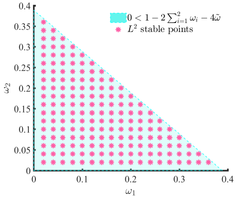
(a) $\tilde{\omega}=1/18$

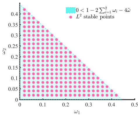
(b) $\tilde{\omega}=1/36$

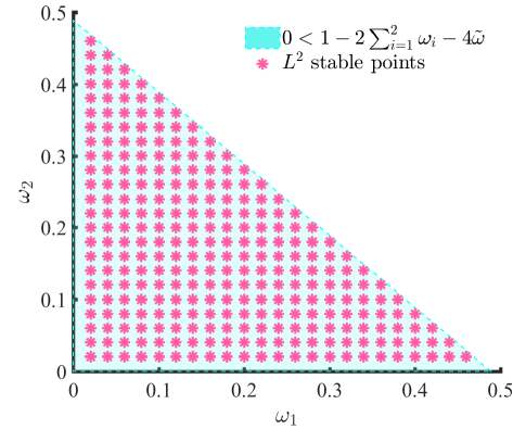
(c) $\tilde{\omega}=1/180$

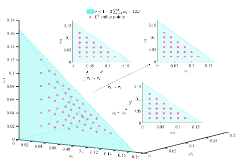
(d) $\tilde{\omega}=1/18$

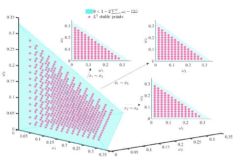
(e) $\tilde{\omega}=1/36$

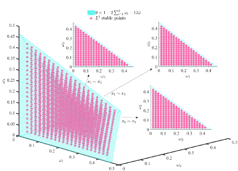
(f) $\tilde{\omega}=1/180$

Figure 1: $L^{2}$ stability regions of the MRT-LB model for the two-dimensional (top) and three-dimensional (bottom) cases under different values of the weight coefficient $\tilde{\omega}$.

3.4 The automatic approach to determine the relaxation parameters and weight coefficients

Based on the above Parts 3.1 and 3.3, it is known that as long as both the fourth-order consistent conditions in (22) and the stability condition in (32) hold, the MRT-LB model (2) for the diagonal-anisotropic diffusion equation (1) can achieve a fourth-order accuracy and is $L^{2}$ stable. In the following, we will discuss how to determine the relaxation parameters and weight coefficients from (22) and (32).

According to (22), one can find that for the general $d$-dimensional case, the choice of $i$ and $j$ is $d(d-1)/2$ in total. In particular, according to the stability condition in (32), similarly, we can take the relaxation parameter $\tilde{s}_{3|x_{i}^{2}x_{j}}$ in (20) as $\tilde{s}_{x_{j}}$. Then, in combination with the fourth-order consistent and $L^{2}$ stability conditions, which can be written as (here we take the choice of $i=j_{1}$ and $j=j_{2}$ as an example)

$$\tilde{g}_{j_{1}}(\eta,\Delta t,s_{x_{j_{1}}},\tilde{s}_{x_{j_{1}}})=0\quad[\makebox{equivalent to (\ref{fourth-coition-1}) for }i=j_{1}],$$ (37a)

$$\tilde{g}_{j_{2}}(\eta,\Delta t,s_{x_{j_{2}}},\tilde{s}_{x_{j_{2}}})=0\quad[\makebox{equivalent to (\ref{fourth-coition-1}) for }i=j_{2}],$$ (37b)

$$g_{j_{1}}(\omega_{j_{1}},\tilde{\omega},\tilde{s}_{x_{j_{1}}})=0\quad[\makebox{equivalent to (\ref{fourth-coition-2}) for }i=j_{1}],$$ (37c)

$$g_{j_{2}}(\omega_{j_{2}},\tilde{\omega},\tilde{s}_{x_{j_{2}}})=0\quad[\makebox{equivalent to (\ref{fourth-coition-2}) for }i=j_{2}],$$ (37d)

$$g_{j_{1}j_{1}}(\omega_{j_{1}},\tilde{\omega},\tilde{s}_{x_{j_{1}}},s_{2|x_{1}^{2}})=0\quad[\makebox{equivalent to (\ref{fourth-coition-3}) and (\ref{condition-stability}) for }i=j_{1}],$$ (37e)

$$g_{j_{2}j_{2}}(\omega_{j_{2}},\tilde{\omega},\tilde{s}_{x_{j_{2}}},s_{2|x_{1}^{2}})=0\quad[\makebox{equivalent to (\ref{fourth-coition-3}) and (\ref{condition-stability}) for }i=j_{2}],$$ (37f)

$$g_{j_{1}j_{2}}(\omega_{j_{1}},\omega_{j_{2}},\tilde{\omega},\tilde{s}_{x_{j_{1}}},\tilde{s}_{x_{j_{2}}},s_{2|x_{1}^{2}},s_{2|x_{j_{1}}x_{j_{2}}})=0\quad[\makebox{equivalent to (\ref{fourth-coition-4}) and (\ref{condition-stability}) for }i=j_{1}\>\>j=j_{2}].$$ (37g)

To solve (37), in this work, we set the proper weight coefficient $\tilde{\omega}\in(0,1)$ and relaxation parameter $s_{2|x_{1}^{2}}\in(0,2)$ in advance, then $s_{x_{j_{1}}}$, $s_{x_{j_{2}}}$, $\omega_{j_{1}}$, $\omega_{j_{2}}$, $\tilde{s}_{x_{j_{1}}}$, $\tilde{s}_{x_{j_{2}}}$, and $s_{2|x_{j_{1}}x_{j_{2}}}$ can be determined by (37a), (37b), (37c), (37d), (37e), (37f), and (37g), respectively. In particular, this solving process can be automated by a simple Matlab symbolic computation code (see B), and after running this code $d(d-1)/2$ times (e.g., x-y, x-z, y-z three groups for the case of $d=3$), all the unknown relaxation parameters and weight coefficients of the MRT-LB model (2) can be determined. To show that the above automatic approach is valid, here we take the two-dimensional case as an example. Specifically, we plot the region of the parameter pair $(\tilde{\epsilon}_{x},\tilde{\epsilon}_{y})$, which represents that the relaxation parameters and weight coefficients can be obtained from (22) and (32), in Fig. 2, where $s_{2|x_{i}^{2}}=1$, $\eta=1$, $\Delta t=1/40$, and different values of the weight coefficient $\tilde{\omega}$ are considered. And from Fig. 2, it can be observed that the region becomes larger as the weight coefficient $\tilde{\omega}$ decreases.

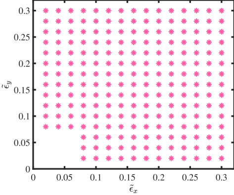
(a) $\tilde{\omega}=1/18$

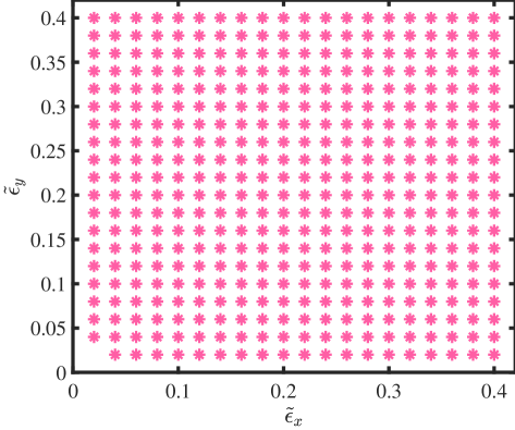
(b) $\tilde{\omega}=1/36$

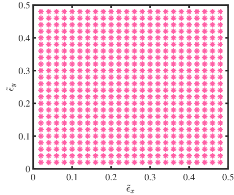
(c) $\tilde{\omega}=1/180$

Figure 2: Regions of the parameter pair $(\tilde{\epsilon}_{x},\tilde{\epsilon}_{y})$ represent that (22) and (32) can be solved under different values of the weight coefficient $\tilde{\omega}$.

Regarding the above discussion on the determination of the relaxation parameters and weight coefficients from (22) and (32), we now give a remark.
Remark 3. As can be seen from (22a) and (22b), the diffusion coefficient $\kappa_{x_{i}}$ is associated with the time step $\Delta t$, except when $s_{x_{i}}=1$. Thus, for the case of $s_{x_{i}}=1$, based on the stability condition (32), we further set $s_{3|x_{i}x_{j}^{2}}=1$ and $s_{2|x_{i}^{2}}=s_{2|x_{1}^{2}}$, (22) can be further simplified as

$$\omega_{i}+2(d-1)\tilde{\omega}=\kappa_{x_{i}}\xi,\quad i\in\llbracket 1,d\rrbracket,$$ (38a)

$$\frac{\omega_{i}+2(d-1)\tilde{\omega}}{4}=\frac{1}{24}-\frac{1}{4}\Big{(}1-\frac{1}{s_{2|x_{1}^{2}}}\Big{)}+\Big{(}\frac{1}{2}-\frac{1}{2s_{2|x_{1}^{2}}}\Big{)}\big{(}\omega_{i}+2(d-1)\tilde{\omega}\big{)},\quad i\in\llbracket 1,d\rrbracket,$$ (38b)

$$\Big{(}\frac{1}{2}+\frac{1}{2s_{2|x_{1}^{2}}}\Big{)}\big{(}\omega_{i}+2(d-1)\tilde{\omega}\big{)}\big{(}\omega_{j}+2(d-1)\tilde{\omega}\big{)}=\Big{(}\frac{2}{s_{2|x_{1}^{2}}}+\frac{4}{s_{2|x_{i}x_{j}}}-5\Big{)}\tilde{\omega},\quad i,j\in\llbracket 1,d\rrbracket,\>\>i<j,$$ (38c)

and it is obvious that the above equation has no solution unless (1) to be solved is reduced to the isotropic type, i.e., the weight coefficient associated with the diffusion coefficient $\kappa_{x_{i}}$ satisfies $\omega_{1}=\omega_{2}=\cdots=\omega_{d}$. Then, the relaxation parameters and weight coefficients can be explicitly obtained from (38) and they are expressed as

$$\omega_{0}=1-2d\omega_{1}-2d(d-1)\tilde{\omega},$$ (39a)

$$\omega_{i}=\epsilon+2\tilde{\omega}-2d\tilde{\omega},\quad i\in\llbracket 1,d\rrbracket,$$ (39b)

$$s_{2|x_{i}^{2}}=\frac{6(2\epsilon-1)}{6\epsilon-5},\quad i\in\llbracket 1,d\rrbracket,$$ (39c)

$$s_{2|x_{i}x_{j}}=-\frac{6\tilde{\omega}(2\epsilon-1)(2\epsilon-1)}{22\epsilon\tilde{\omega}-\epsilon^{2}-5\tilde{\omega}+2\epsilon^{3}-24\epsilon^{2}\tilde{\omega}}\quad i,j\in\llbracket 1,d\rrbracket,\>\>j\neq i,$$ (39d)

where $\epsilon\overset{\Delta}{=}\epsilon_{x_{i}}=\tilde{\epsilon}_{x_{i}}$ for all $i\in\llbracket 1,d\rrbracket$. This indicates that for the isotropic diffusion equation, the relaxation parameters and weight coefficients, which are used to ensure that the MRT-LB model (2) is fourth-order accurate and $L^{2}$ stable, are not unique. They can be either automatically obtained from (37) without any other restrictions or given by (39) with $s_{x_{i}}=1$. In addition, we would also like to point out that for the isotropic diffusion equation, the fourth-order consistent condition (23) of the MRT-LB model with the D$d$Q($2d+1$) lattice structure in Remark 2 can also be explicitly solved, and the solution is given by

$$\omega_{i}=1-4\sqrt{3}\epsilon,\quad i\in\llbracket 1,d\rrbracket,$$ (40a)

$$s_{x_{i}}=\frac{2\Delta t\eta}{\Delta t\eta-\sqrt{(\tilde{s}_{x_{i}}-4\Delta t\eta+\Delta t^{2}\tilde{s}_{x_{i}}\eta^{2}+2\Delta t\tilde{s}_{x_{i}}\eta)/\tilde{s}_{x_{i}}}+1},\quad i\in\llbracket 1,d\rrbracket,$$ (40b)

$$s_{2|x_{i}^{2}}=4\sqrt{3}-6,\quad i\in\llbracket 1,d\rrbracket,$$ (40c)

where $\tilde{s}_{x_{i}}=6/(3+\sqrt{3})$ for all $i\in\llbracket 1,d\rrbracket$.

4 Numerical results and discussion

In this section, we will conduct two benchmarks to test the numerical accuracy of the present MRT-LB model (2) for the diagonal-anisotropic diffusion equation (1), where the relaxation parameters and weight coefficients are given by the proposed automatic approach (see Parts 3.4 and B), and the numerical accuracy is determined based on the following relative error in $l^{2}$-norm,

$$l^{2}(\phi)=\sqrt{\frac{\sum_{i}\phi(\mathbf{x}_{i},t_{n})-\phi^{\star}(\mathbf{x}_{j},t_{n})}{\sum_{i}\big{(}\phi^{\star}(\mathbf{x}_{i},t_{n})\big{)}^{2})}},$$

where $\phi(\mathbf{x}_{j},t_{n})$ and $\phi^{\star}(\mathbf{x}_{j},t_{n})$ represent the numerical and analytical solutions at lattice node $\mathbf{x}_{j}$ ad time $t_{n}$.

4.1 Gauss Hill in two-, three-, and four-dimensional cases

The first example considers the Gauss Hill problem, and the initial condition is expressed as

$$\phi(\mathbf{x},0)=\frac{\phi_{0}}{2\pi|\Gamma_{0}|}\exp\Big{(}-\frac{\mathbf{x}^{2}}{2\Gamma_{0}^{2}}\Big{)}.$$

With the periodic boundary condition, one can obtain the analytical solution of this problem,

$$\phi^{\star}(\mathbf{x},t)=\frac{\phi_{0}}{2\pi|\det(\Gamma)|^{1/2}}\exp\Bigg{(}-\frac{\sum_{i,j=1}^{d}(\Gamma^{-1})_{ij}(\mathbf{x}\mathbf{x}^{T})_{ij}}{2}\Bigg{)},$$

where $\Gamma=\Gamma_{0}^{2}\mathbf{I}+\bm{\kappa}t\in\mathbb{R}^{d\times d}$ [$\bm{\kappa}=\makebox{{diag}}(\kappa_{x_{1}},\kappa_{x_{2}},\cdots,\kappa_{x_{d}})$ with $d=2,3$, and 4] and $\det(\Gamma)$ represents the determinant values of $\Gamma$. In the following simulations, the computational domain is set to be $[-1,1]^{d}$ and the total concentration $\phi_{0}$ is taken as $\phi_{0}=2\pi\Gamma_{0}$, where $\Gamma_{0}$ should be small enough to ensure that the periodic boundary condition makes sense, and we here consider it as 0.05.

In order to show the performance of the present MRT-LB model, we first conduct some tests with different values of the diagonal diffusion matrix $\bm{\kappa}$ in two-dimensional case, where the lattice spacing $\Delta x=1/100$, the time step $\Delta t=1/40$, and the weight coefficients and relaxation parameters are presented in Table 1. The contour lines of the numerical and analytical solutions at the final time $t=2$ are plotted in Fig. 3, from which one can find that the numerical results of the MRT-LB model are in good agreement with the analytical solutions.

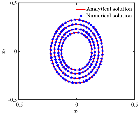
(a) $(\epsilon_{x_{1}},{\epsilon}_{x_{2}})=(0.40,0.10)$

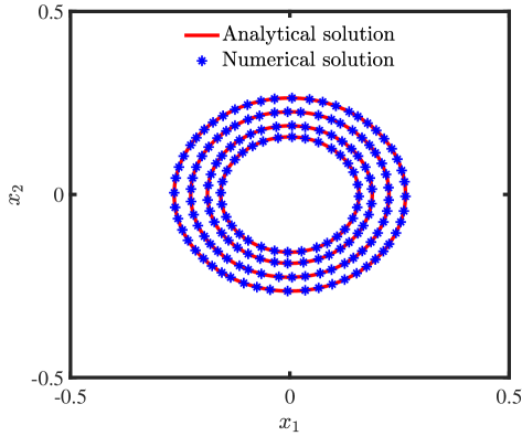
(b) $(\epsilon_{x_{1}},{\epsilon}_{x_{2}})=(0.20,0.20)$

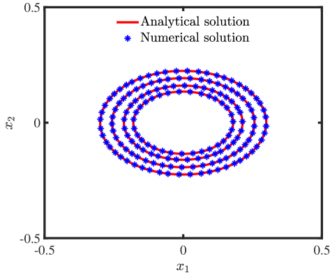
(c) $(\epsilon_{x_{1}},{\epsilon}_{x_{2}})=(0.10,0.30)$

Figure 3: Contour lines of the numerical and analytical solutions under different values of the parameter pair $(\epsilon_{x_{1}},{\epsilon}_{x_{2}})$.

Then, to investigate the impact of the initialization scheme on the accuracy of the MRT-LB model, for the Gauss Hill in all the two-, three-, and four-dimensional cases, we test the convergence rates of the present MRT-LB model with different initialization schemes of $f_{k}=f_{k}^{eq}$ and (24). The results are presented in Fig. 4, where $(\epsilon_{x_{1}},\epsilon_{x_{2}})=(0.30,0.10)$, $(\epsilon_{x_{1}},\epsilon_{x_{2}},\epsilon_{x_{3}})=(0.10,0.40,0.15)$, $(\epsilon_{x_{1}},\epsilon_{x_{2}},\epsilon_{x_{3}},\epsilon_{x_{4}})=(0.15,0.20,0.10,0.05)$, and the values of relaxation parameters and weight coefficients for $d=3$ and 4 are provided in Table 1. From this figure, we can clearly see that when the distribution function is initialized at the equilibrium state $f_{k}^{eq}$, the MRT-LB model only achieves a second-order accuracy. However, when the initialization scheme in (24) is adopted, the MRT-LB model can be fourth-order accurate, which is in full agreement with our theoretical analysis in Part 3.2.

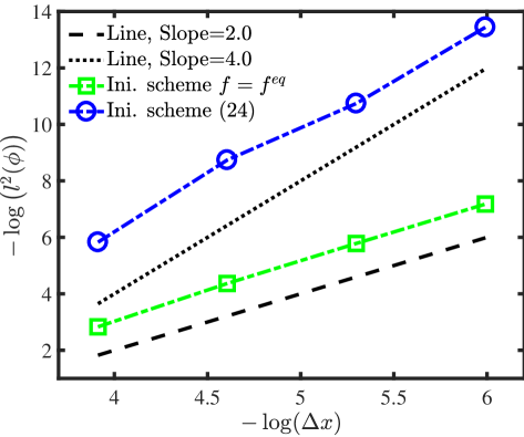
(a) $d=2(\Delta x^{2}/\Delta t=1/250)$

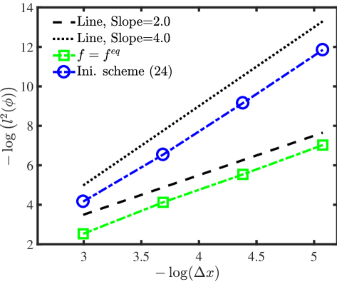
(b) $d=3(\Delta x^{2}/\Delta t=1/40)$

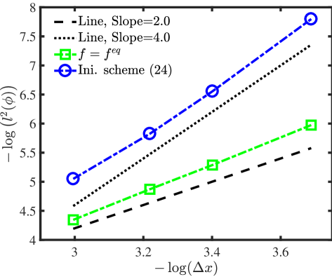
(c) $d=4(\Delta x^{2}/\Delta t=1/50)$

Figure 4: Convergence rates of the MRT-LB model with different initialization schemes at the final time $t=2$.

Table 1: Relaxation parameters and weight coefficients of the MRT-LB model for $d=2$, 3, and 4.

$({\epsilon}_{x_{1}},{\epsilon}_{x_{2}},\cdots,{\epsilon}_{x_{d}})$	$(0.40,0.10)$	$(0.20,0.20)$	$(0.10,0.30)$	$(0.10,0.40,0.15)$	$(0.15,0.20,0.10,0.05)$
$\omega_{0}$	0.392414074930637	0.466081465800228	0.279164263737521	0.044310556197977	0.003107936020711
$\omega_{1}$	0.003792962534682	0.105701855772165	11/45	1/9	0.148170462855893
$\omega_{2}$	11/45	0.105701855772165	0.060417868131240	0.037126295868015	0.144590744661054
$\omega_{3}$	-	-	-	0.296273981588552	0.116666666666667
$\omega_{4}$	-	-	-	-	0.055684824472697
$\tilde{\omega}$	1/36	1/36	1/36	1/180	1/360
$s_{x_{1}}$	0.258403002308493	0.892756279989137	3/2	8/7	1.047126365130629
$s_{x_{2}}$	3/2	0.892756279989137	0.557600159447285	0.258403002308493	0.892756279989137
$s_{x_{3}}$	-	-	-	1.359653295886320	1.142857142857143
$s_{x_{4}}$	-	-	-	-	1.182682621447616
$s_{2|x_{1}^{2}}$	1	1	1	1	1
$s_{2|x_{1}x_{2}}$	1.466835061000191	1.011385583524664	1.192683097984767	0.945790034643835	0.299130236472667
$s_{2|x_{1}x_{3}}$	-	-	-	1.151202850452001	0.485974551112802
$s_{2|x_{1}x_{4}}$	-	-	-	-	0.696896856214742
$s_{2|x_{2}x_{3}}$	-	-	-	0.770241927190338	0.408239754101923
$s_{2|x_{2}x_{4}}$	-	-	-	-	0.625878745350766
$s_{2|x_{3}x_{4}}$	-	-	-	-	0.812554973056151

4.2 Diagonal-anisotropic diffusion equation with a linear source

In the second example, we focus on the two-dimensional diagonal-anisotropic diffusion equation (1) with a linear source term, in which the initial condition is given by

$$\phi(x,y,0)=\sin(\pi x)\sin(\pi y)+\pi^{2},\quad(x,y)\in(-1,1)\times(-1,1),$$

and the analytical solution can be obtained as

$$\phi^{\star}(x,y,t)=\sin(\pi x)\sin(\pi y)\exp\Big{[}\big{(}-\pi^{2}(\kappa_{x}+\kappa_{y}+1)\big{)}\Big{]}.$$

First of all, we consider three different values of the parameter pair $(\tilde{\epsilon}_{x},\tilde{\epsilon}_{y})=(0.25,0.10)$, $(0.40,0.40)$, and $(0.15,0.40)$. For the MRT-LB model, the weight coefficient $\tilde{\omega}=1/36$, the relaxation parameter $s_{2|x_{i}^{2}}=1$, and the other weight coefficients and relaxation parameters can be seen in Table 2. Fig. 5 plots the profiles of the numerical results at different values of the final time $t$, where the lattice spacing $\Delta x=1/80$ and the time step $\Delta t=1/400$. From Fig. 5, one can see that the numerical results are in good agreement with the analytical solutions. In addition, the logarithm of the relative errors at the final time $t=1$ with respect to the lattice spacing $\Delta x$ is also shown in Fig. 6, where the time step $\Delta t$ is given by the relation $\Delta x^{2}/\Delta t=1/16$. From this figure, it can be seen that for the diagonal-anisotropic diffusion equation with a linear source term, the present MRT-LB model can also be fourth-order accurate, which is consistent with our theoretical analysis.

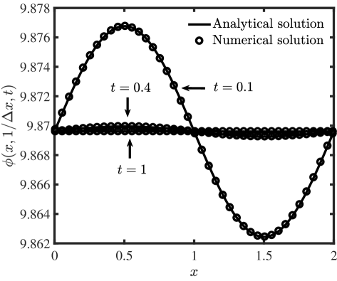
(a) $(\tilde{\epsilon}_{x},\tilde{\epsilon}_{y})=(0.25,0.10)$

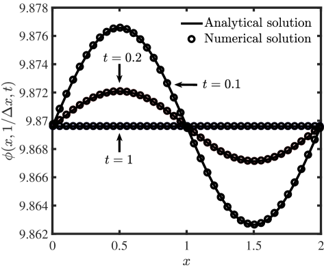
(b) $(\tilde{\epsilon}_{x},\tilde{\epsilon}_{y})=(0.40,0.40)$

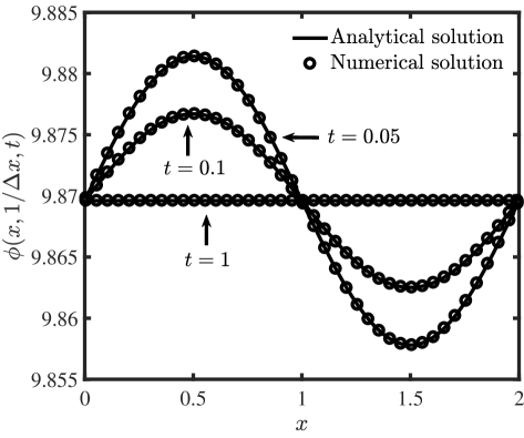
(c) $(\tilde{\epsilon}_{x},\tilde{\epsilon}_{y})=(0.15,0.40)$

Figure 5: Profiles of the numerical and analytical solutions under different values of the final time $t$.

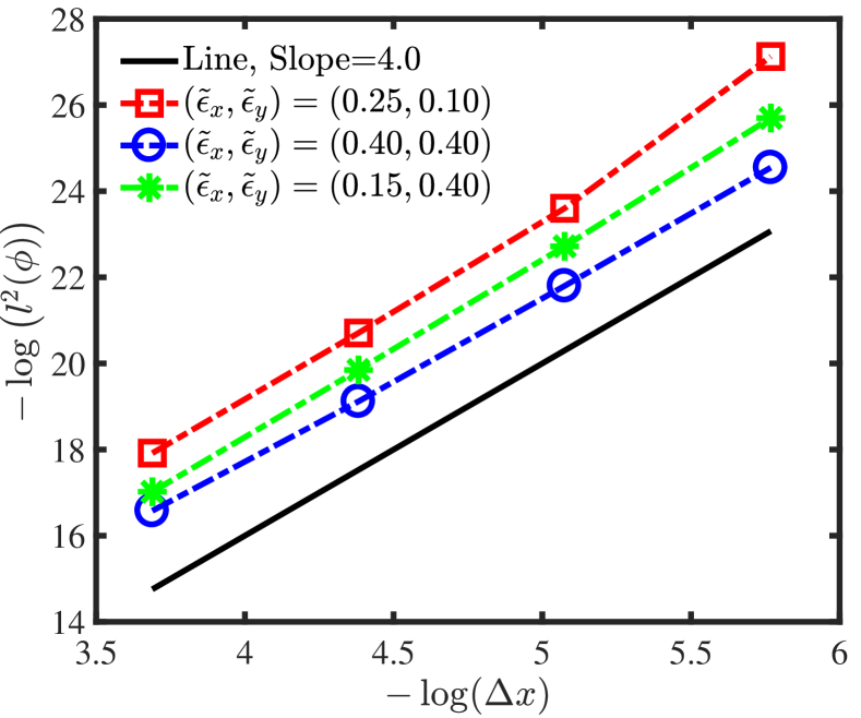
Figure 6: Convergence rates of the MRT-LB model under different values of the parameter pair ($\tilde{\epsilon}_{x},\tilde{\epsilon}_{y}$).

Table 2: Relaxation parameters and weight coefficients of the MRT-LB model under different values of the parameter pair $(\tilde{\epsilon}_{x},\tilde{\epsilon}_{y})$.

$(\tilde{\epsilon}_{x},\tilde{\epsilon}_{y})$	$(0.25,0.10)$	$(0.40,0.40)$	$(0.15,0.40)$
$\omega_{0}$	0.228240384066444	0.873717038750163	0.662739815885518
$\omega_{1}$	0.085879807966778	0.003792962534682	0.109281573967004
$\omega_{2}$	11/45	0.003792962534682	0.003792962534682
$s_{x}$	0.729269281934827	0.314095759114162	1.045990365920910
$s_{y}$	1.487864247860460	0.314095759114162	0.275195555816491
$s_{2|xy}$	1.114757496216724	1.770421857439279	1.468455215964528

Then, when the diagonal-anisotropic diffusion equation is reduced to the isotropic type, i.e., $\tilde{\epsilon}_{x}=\tilde{\epsilon}_{y}$, a simulation is conducted to give a comparison of the fourth-order MRT-LB-D2Q9-(37) , MRT-LB-D2Q9-(39) , and MRT-LB-D2Q5-(40) models. Considering two different values of the parameter $\tilde{\epsilon}_{x}=0.1$ and $0.2$, we measure the relative errors of these three models and calculate the convergence rates (CRs) in Table 4, where the final time $t=1$ and the weight coefficients and relaxation parameters of these three models are provided in Table 3. From Table 4 with the parameter $\tilde{\epsilon}_{x}=0.1$, one can find that all the three MRT-LB models have a fourth-order accuracy, which is in agreement with our theoretical analysis in Remark 3. However, for the case of $\tilde{\epsilon}_{x}=0.2$ shown in Table 4, both the MRT-LB-D2Q9-(37) and MRT-LB-D2Q9-(39) models can achieve a fourth-order accuracy while the MRT-LB-D2Q5-(40) model cannot. This is due to the fact that, as can be seen in Table 3, the weight coefficient $\omega_{0}<0$ of the MRT-LB-D2Q5-(40) model, which means that the MRT-LB-D2Q5-(40) model is no longer stable for the case of $\tilde{\epsilon}_{x}=0.2$. Therefore, we can conclude that for the isotropic diffusion equation, the fourth-order MRT-LB model with the D$d$Q($2d^{2}+1$) lattice structure is more general than that with the D$d$Q($2d+1$) lattice structure .

Table 3: Relaxation parameters and weight coefficients of the MRT-LB-D2Q9-(37), MRT-LB-D2Q9-(39), and MRT-LB-D2Q5-(40) models.

Model	MRT-LB-D2Q9-(37)			MRT-LB-D2Q9-(39)			MRT-LB-D2Q5-(40)
$\tilde{\epsilon}_{x}$	0.1	0.2		0.1	0.2		0.1	0.2
$\omega_{0}$	4/9	4/9		32/45	14/45		$1-0.4\sqrt{3}$	$(1-0.8\sqrt{3})<0$
$\omega_{1}=\omega_{2}$	1/9	1/9		2/45	13/90		$0.1\sqrt{3}$	$0.2\sqrt{3}$
$\tilde{\omega}$	1/36	1/36		1/36	1/36		-	-
$s_{x_{1}}=s_{x_{2}}$	1.227162705974765	0.917191588597811		1	1		1.243448367507882	1.261464647585203
$s_{2|x_{1}^{2}}=s_{2|x_{2}^{2}}$	1	1		12/11	18/19		$4\sqrt{3}-6$	$4\sqrt{3}-6$
$s_{2|x_{1}x_{2}}$	0.948397105014222	0.993142767001046		15/13	90/101		-	-

Table 4: Relative errors and convergence rates of the MRT-LB-D2Q9-(37), MRT-LB-D2Q9-(39), and MRT-LB-D2Q5-(40) models under different values of the parameter $\tilde{\epsilon}_{x}$.

$\tilde{\epsilon}_{x}$	$\Delta x$	MRT-LB-D2Q9-(37)			MRT-LB-D2Q9-(39)			MRT-LB-D2Q5-(40)
		$l^{2}(\phi)$	CR		$l^{2}(\phi)$	CR		$l^{2}(\phi)$	CR
0.1	1/40	1.8240$\times 10^{-8}$	-		1.8101$\times 10^{-8}$	-		1.8539$\times 10^{-8}$	-
	1/80	1.1344$\times 10^{-9}$	3.9961		1.1614$\times 10^{-9}$	3.9966		1.1318$\times 10^{-9}$	3.9958
	1/160	7.0916$\times 10^{-11}$	3.9996		7.2597$\times 10^{-11}$	3.9998		7.0760$\times 10^{-11}$	3.9996
	1/240	1.4008$\times 10^{-11}$	3.9999		1.4340$\times 10^{-11}$	4.0000		1.3978$\times 10^{-11}$	3.9999
	1/320	4.4324$\times 10^{-12}$	4.0000		4.5375$\times 10^{-12}$	3.9999		4.4227$\times 10^{-12}$	4.0000
0.2	1/40	1.6813$\times 10^{-8}$	-		1.6331$\times 10^{-8}$	-		0.9895	-
	1/80	1.0549$\times 10^{-9}$	3.9944		1.0232$\times 10^{-9}$	3.9965		1.0000	-0.0152
	1/160	6.5971$\times 10^{-11}$	3.9992		6.3962$\times 10^{-11}$	3.9998		-	-
	1/240	1.3032$\times 10^{-11}$	3.9998		1.2634$\times 10^{-11}$	4.0000		-	-
	1/320	4.1237$\times 10^{-12}$	3.9999		3.9976$\times 10^{-12}$	4.0000		-	-

5 Conclusion

This work proposes an automatic approach to determine the fourth-order and $L^{2}$ stable MRT-LB model for the diagonal-anisotropic diffusion equation, in which the MRT-LB model adopts the transformation matrix constructed in a natural way and the D$d$Q($2d^{2}+1$) lattice structure.

• Through the direct Taylor expansion, the conditions, which are associated with the relaxation parameters and weight coefficients, are derived to ensure that the macroscopic modified equation of the MRT-LB model can be fourth-order consistent with the diagonal-anisotropic diffusion equation. In particular, for the isotropic diffusion equation, another MRT-LB model with the D$d$Q($2d+1$) lattice structure [fewer discrete velocities than the D$d$Q($2d^{2}+1$) lattice structure] is developed, and the fourth-order consistent conditions are also similarly given. Furthermore, to obtain an overall fourth-order MRT-LB model, the fourth-order initialization scheme of the distribution function is also constructed.

• The condition which guarantees that the present MRT-LB model can satisfy the stability structure is given. In particular, once the stability structure is satisfied, it can be numerically validated that the MRT-LB model is $L^{2}$ stable. Then, based on this stability structure preserving condition and the above fourth-order consistent conditions, the relaxation parameters and weight coefficients of the MRT-LB model can be automatically determined by a simple computer code.

• Some numerical experiments are carried out to test the convergence rate of the proposed MRT-LB model, and the numerical results are consistent with our theoretical analysis. In addition, a comparison simulation is conducted with respect to the isotropic diffusion equation, and the numerical results show that compared with the fourth-order MRT-LB model with the D$d$Q($2d+1$) lattice structure, the present fourth-order MRT-LB model with the D$d$Q($2d^{2}+1$) lattice structure is more general.

In summary, for the general diagonal-anisotropic diffusion equation, after obtaining the relaxation parameters and weight coefficients by a simple computer code, the MRT-LB model is fourth-order accurate, $L^{2}$ stable, and also valid for the high-dimensional case.

Appendix A The second- to fifth-order expansions of the distribution function

To obtain the second- to fifth-order expansions of the distribution function $f_{k}$, we here divide the derivation into four steps.

A.1 The second-order expansion

Substituting $f_{k}^{ne}=O(\Delta x)$ into (3.1) yields the following second-order expansion of the distribution function $f_{k}$,

$$O(\Delta x^{2})+\Delta x\mathbf{e}_{k}\cdot\nabla f_{k}^{eq}=-\sum_{i=1}^{q}\mathbf{\Lambda}_{ki}f_{i}^{ne}.$$ (41)

A.2 The third-order expansion

Based on the above (41), one can obtain the third-order expansion of the distribution function $f_{k}$ from (3.1),

$$\xi\Delta x^{2}\partial_{t}f_{k}^{eq}+\Delta x\mathbf{e}_{k}\cdot\nabla f_{k}^{eq}-\Delta x^{2}\nabla^{2}\overset{2}{\cdot}\mathbf{e}_{k}\sum_{i=1}^{q}\bm{\Lambda}^{-1}_{ki}\mathbf{e}_{i}f_{i}^{eq}+\frac{\Delta x^{2}}{2}\nabla^{2}\overset{2}{\cdot}\mathbf{e}_{k}^{2}f_{k}^{eq}$$

$$-\xi\Delta x^{2}\sum_{i=1}^{q}\Big{(}\mathbf{I}-\frac{\mathbf{\Lambda}}{2}\Big{)}_{ki}R_{i}+O(\Delta x^{3})=-\sum_{i=1}^{q}\mathbf{\Lambda}_{ki}f_{i}^{ne}.$$ (42)

A.3 The fourth-order expansion

From (3.1), the fourth-order expansion of the distribution function $f_{k}$ is given by

$$\xi\Delta x^{2}\partial_{t}f_{k}^{eq}-\xi\Delta x^{3}\sum_{i=1}^{q}\mathbf{\Lambda}_{ki}^{-1}\mathbf{e}_{i}\cdot\nabla\partial_{t}f_{i}^{eq}+O(\Delta x^{4})=-\Delta x\mathbf{e}_{k}\cdot\nabla f_{k}^{eq}+\frac{\Delta x^{2}}{2}\mathbf{e}_{k}^{2}\overset{2}{\cdot}\nabla^{2}f_{k}^{eq}-\Delta x^{2}\nabla^{2}\overset{2}{\cdot}\mathbf{e}_{k}\sum_{i=1}^{q}\Big{(}\mathbf{I}-\bm{\Lambda}^{-1}\Big{)}_{ki}\mathbf{e}_{i}f_{i}^{eq}$$

$$-\sum_{i=1}^{q}\mathbf{\Lambda}_{ki}f_{i}^{ne}-\xi\Delta x^{3}\nabla\cdot\mathbf{e}_{k}\sum_{i=1}^{q}\Big{(}\mathbf{I}-\bm{\Lambda}^{-1}\Big{)}_{ki}\partial_{t}f_{i}^{eq}$$

$$-\Delta x\nabla^{3}\overset{3}{\cdot}\mathbf{e}_{k}\sum_{i=1}^{q}\bigg{(}\bm{\Lambda}^{-1}_{ki}\mathbf{e}_{i}\sum_{l=1}^{q}\Big{(}\bm{\Lambda}^{-1}_{il}\mathbf{e}_{l}f_{l}^{eq}\Big{)}\bigg{)}+\frac{\Delta x^{3}}{2}\nabla^{3}\overset{3}{\cdot}\mathbf{e}_{k}\sum_{i=1}^{q}\bm{\Lambda}^{-1}_{ki}\mathbf{e}^{2}_{i}f_{i}^{eq}+\frac{\Delta x^{3}}{2}\nabla^{3}\overset{3}{\cdot}\mathbf{e}_{k}^{2}\sum_{i=1}^{q}\bm{\Lambda}^{-1}_{ki}\mathbf{e}_{i}f_{i}^{eq}-\frac{\Delta x^{3}}{6}\nabla^{3}\overset{3}{\cdot}\mathbf{e}_{k}^{3}f_{k}^{eq}$$

$$+\xi\Delta x^{2}\sum_{i=1}^{q}\Big{(}\mathbf{I}-\frac{\mathbf{\Lambda}}{2}\Big{)}_{ki}R_{i}-\xi\Delta x^{3}\mathbf{e}_{k}\cdot\nabla\sum_{i=1}^{q}\Big{(}\mathbf{\Lambda}^{-1}-\frac{\mathbf{I}}{2}\Big{)}_{ki}R_{i},$$ (43)

where (41) and (A.2) have been used. After taking the second-order moment of the above equation, one can obtain the unknown term $\sum_{k=1}^{q}\mathbf{e}_{ki}\mathbf{e}_{kj}f_{k}^{ne}$ [see (14b)].

A.4 The fifth-order expansion

According to (41), (A.2), and (A.3), we can further obtain the fifth-order expansion of the distribution function $f_{k}$ from (3.1),

$$\xi\Delta x^{2}\partial_{t}f_{k}^{eq}-\xi\Delta x^{2}\partial_{t}\sum_{i=1}^{q}\bm{\Lambda}^{-1}_{ki}\Big{(}\xi\Delta x^{2}\partial_{t}f_{i}^{eq}+\Delta x\mathbf{e}_{i}\cdot\nabla f_{i}^{eq}-\Delta x^{2}\nabla^{2}\overset{2}{\cdot}\mathbf{e}_{i}\sum_{l=1}^{q}\bm{\Lambda}^{-1}_{il}\mathbf{e}_{l}f_{l}^{eq}+\frac{\Delta x^{2}}{2}\nabla^{2}\overset{2}{\cdot}\mathbf{e}_{i}^{2}f_{i}^{eq}$$

$$\qquad\qquad\qquad\qquad\qquad\quad-\xi\Delta x^{2}\sum_{i=1}^{q}\Big{(}\mathbf{I}-\frac{\mathbf{\Lambda}}{2}\Big{)}_{ki}R_{i}\Big{)}+\frac{\xi^{2}\Delta x^{4}}{2}\partial_{t}^{2}f_{k}^{eq}+O(\Delta x^{5})$$

$$=-\Delta x\mathbf{e}_{k}\cdot\nabla f_{k}^{eq}+\frac{\Delta x^{2}}{2}\mathbf{e}_{k}^{2}\overset{2}{\cdot}\nabla^{2}f_{k}^{eq}-\frac{\Delta x^{3}}{6}\mathbf{e}_{k}^{3}\overset{3}{\cdot}\nabla^{3}f_{k}^{eq}+\frac{\Delta x^{4}}{24}\mathbf{e}_{k}^{4}\overset{4}{\cdot}\nabla^{4}f_{k}^{eq}-\sum_{i=1}^{q}\mathbf{\Lambda}_{ki}f_{i}^{ne}$$

$$-\Delta x\mathbf{e}_{k}\cdot\nabla\sum_{i=1}^{q}\Big{(}\mathbf{I}-\mathbf{\Lambda}^{-1}\Big{)}_{ki}\Bigg{(}\xi\Delta x^{2}\partial_{t}f_{i}^{eq}-\xi\Delta x^{3}\sum_{l=1}^{q}\bm{\Lambda}^{-1}_{il}\mathbf{e}_{l}\cdot\nabla\partial_{t}f_{l}^{eq}+\Delta x\mathbf{e}_{i}\cdot\nabla f_{i}^{eq}-\frac{\Delta x^{2}}{2}\mathbf{e}_{i}^{2}\overset{2}{\cdot}\nabla^{2}f_{i}^{eq}$$

$$\qquad\qquad\qquad\qquad\qquad\quad+\Delta x^{2}\nabla^{2}\overset{2}{\cdot}\mathbf{e}_{i}\sum_{l=1}^{q}\Big{(}\mathbf{I}-\mathbf{\Lambda}^{-1}\Big{)}_{il}\mathbf{e}_{l}f_{l}^{eq}+\xi\Delta x^{3}\nabla\cdot\mathbf{e}_{i}\sum_{l=1}^{q}\Big{(}\mathbf{I}-\mathbf{\Lambda}^{-1}\Big{)}_{il}\partial_{t}f_{l}^{eq}$$

$$\qquad\qquad\qquad\qquad\qquad\quad+\Delta x^{3}\nabla^{3}\overset{3}{\cdot}\mathbf{e}_{i}\sum_{l=1}^{q}\mathbf{\Lambda}^{-1}_{il}\mathbf{e}_{l}\sum_{o=1}^{q}\mathbf{\Lambda}^{-1}_{lo}\mathbf{e}_{o}f_{o}^{eq}-\frac{\Delta x^{3}}{2}\nabla^{3}\overset{3}{\cdot}\mathbf{e}_{i}\sum_{l=1}^{q}\mathbf{\Lambda}^{-1}_{il}\mathbf{e}_{l}^{2}f_{l}^{eq}-\frac{\Delta x^{3}}{2}\nabla^{3}\overset{3}{\cdot}\mathbf{e}_{i}^{2}\sum_{l=1}^{q}\mathbf{\Lambda}_{il}^{-1}\mathbf{e}_{l}f_{l}^{eq}$$

$$\qquad\qquad\qquad\qquad\qquad\quad+\frac{\Delta x^{3}}{6}\nabla^{3}\overset{3}{\cdot}\mathbf{e}_{i}^{3}f_{i}^{eq}+\xi\Delta x^{3}\nabla\cdot\mathbf{e}_{i}\sum_{l=1}^{q}\Big{(}\mathbf{\Lambda}^{-1}-\frac{\mathbf{I}}{2}\Big{)}_{il}R_{l}-\xi\Delta x^{2}\sum_{l=1}^{q}\Big{(}\mathbf{I}-\frac{\mathbf{\Lambda}}{2}\Big{)}_{il}R_{l}\Bigg{)}$$

$$+\frac{\Delta x^{2}}{2}\mathbf{e}_{k}^{2}\overset{2}{\cdot}\nabla^{2}\sum_{i=1}^{q}\Big{(}\mathbf{I}-\mathbf{\Lambda}^{-1}\Big{)}_{ki}\bigg{(}\xi\Delta x^{2}\partial_{t}f_{i}^{eq}+\Delta x\mathbf{e}_{k}\cdot\nabla f_{i}^{eq}-\Delta x^{2}\nabla^{2}\overset{2}{\cdot}\mathbf{e}_{i}\sum_{l=1}^{q}\mathbf{\Lambda}^{-1}_{il}\mathbf{e}_{l}f_{l}^{eq}$$

$$\qquad\qquad\qquad\qquad\qquad\qquad+\frac{\Delta x^{2}}{2}\mathbf{e}_{i}^{2}\overset{2}{\cdot}\nabla^{2}f_{i}^{eq}-\xi\Delta x^{2}\sum_{l=1}^{q}\Big{(}\mathbf{I}-\frac{\mathbf{\Lambda}}{2}\Big{)}_{il}R_{l}\bigg{)}$$

$$-\frac{\Delta x^{4}}{6}\nabla^{4}\overset{4}{\cdot}\mathbf{e}_{k}^{3}\sum_{i=1}^{q}\Big{(}\mathbf{I}-\mathbf{\Lambda}^{-1}\Big{)}_{ki}\mathbf{e}_{i}f_{i}^{eq}$$

$$+\xi\Delta x^{2}\sum_{i=1}^{q}\Big{(}\mathbf{I}-\frac{\mathbf{\Lambda}}{2}\Big{)}_{ki}R_{i}-\xi\Delta x^{3}\mathbf{e}_{k}\cdot\nabla\sum_{i=1}^{q}\Big{(}\mathbf{I}-\frac{\mathbf{\Lambda}}{2}\Big{)}_{ki}R_{i}+\frac{\xi\Delta x^{4}}{2}\nabla^{2}\overset{2}{\cdot}\mathbf{e}_{k}^{2}\sum_{i=1}^{q}\Big{(}\mathbf{I}-\frac{\mathbf{\Lambda}}{2}\Big{)}_{ki}R_{i}.$$ (44)

And the unknown term $\sum_{k=1}^{q}\mathbf{e}_{ki}f_{k}^{ne}$ can be determined by taking the first-order moment of the above equation [see (14a)].

Appendix B The Matlab symbolic computation code

We here provide a simple code to determine the relaxation parameters and weight coefficients of the fourth order MRT-LB model (2) for the diagonal-anisotropic diffusion equation (1). To use the code for a high-dimensional case, one only needs to run the following code for each group consisting of two different directions, and the relaxation parameters and weight coefficients will be determined by the code output.

function  [w$\_$xi,w$\_$xj,s$\_$xi,s$\_$xj,s$\_$xixj,s$\_$xi2xj,s$\_$xixj2]  …

$=$ Fun$\_$LB$\_$relax$\_$para(ww,d,s2i,eta,dt,dx,kappa$\_$xi,kappa$\_$xj)

syms  sij si  sj  wi wj real;

s$\_$2j $=$ s$\_$2i;  si2j $=$ sj; sij2 $=$ si;

epsilon$\_$i $=$ kappa$\_$xi*dt/dx² ;

epsilon$\_$j $=$ kappa$\_$xj*dt/dx² ;

eqi $=$ epsilon$\_$i $-$ (1/si $-$ 1/2)*(2*wi $+$ 4*(d $-$ 1)*ww);

eqj $=$ epsilon$\_$j $-$ (1/sj $-$ 1/2)*(2*wj $+$ 4*(d $-$ 1)*ww);

eqii $=$ ((1/2*epsilon$\_$i*(1/si $-$ 1/2)-  …

( 1/3/si $-$ 7/24 $+$ (1/si/s2i $-$ 1/2/si $-$ 1/2/s2i)*(1/si $-$ 1) $-$ 1/2*(1 $-$ 1/s2i)*(1/si $-$ 1/2)  …

$+$ ((1/si $-$ 1)*(1 $-$ 1/s2i $-$ 1/si) $+$ 1/2 $-$ 1/2/s2i)*epsilon$\_$i))/(1/si $-$ 1/2));

eqjj $=$ ((1/2*epsilon$\_$j*(1/sj $-$ 1/2) $-$  …

( 1/3/sj $-$ 7/24 $+$ (1/sj/s2j $-$ 1/2/sj $-$ 1/2/s2j)*(1/sj $-$ 1) $-$ 1/2*(1 $-$ 1/s2j)*(1/sj $-$ 1/2)  …

$+$ ((1/sj $-$ 1)*(1 $-$ 1/s2j $-$ 1/sj) $+$ 1/2 $-$ 1/2/s2j)*epsilon$\_$j ))/(1/sj $-$ 1/2));

eqij $=$ (epsilon$\_$i*epsilon$\_$j $-$  …

( 4*( $-$ 7/24 $+$ 1/6/si $+$ (1/si2j/s2i $-$ 1/2/si2j $-$ 1/2/s2i)*(1/si $-$ 1) …

$-$ 1/2*(1 $-$ 1/s2i)*(1/si2j $-$ 1/2) $+$ 1/6/si2j)*ww  …

$+$ 4*( $-$ 7/24 $+$ 1/6/sj $+$ (1/sij2/s2j $-$ 1/2/sij2 $-$ 1/2/s2j)*(1/sj $-$ 1) …

$-$ 1/2*(1 $-$ 1/s2j)*(1/sij2 $-$ 1/2) $+$ 1/6/sij2)*ww …

$+$ 4*( $-$ 7/24 $+$ 1/6/si $+$ (1/si2j/sij $-$ 1/2/si2j $-$ 1/2/sij)*(1/si $-$ 1) …

$-$ 1/2*(1 $-$ 1/sij)*(1/si2j $-$ 1/2) $+$ 1/6/si2j)*ww  …

$+$ 4*( $-$ 7/24 $+$ 1/6/sj $+$ (1/sij2/sij $-$ 1/2/sij2 $-$ 1/2/sij)*(1/sj $-$ 1) …

$-$ 1/2*(1 $-$ 1/sij)*(1/sij2 $-$ 1/2) $+$ 1/6/sij2)*ww …

$+$ 4*( $-$ 7/24 $+$ 1/6/si $+$ (1/sij2/sij $-$ 1/2/sij2 $-$ 1/2/sij)*(1/si $-$ 1) …

$-$ 1/2*(1 $-$ 1/sij)*(1/sij2 $-$ 1/2) $+$ 1/6/sij2)*ww  …

$+$ 4*( $-$ 7/24 $+$ 1/6/sj $+$ (1/si2j/sij $-$ 1/2/si2j $-$ 1/2/sij)*(1/sj $-$ 1) …

$-$ 1/2*(1 $-$ 1/sij)*(1/si2j $-$ 1/2) $+$ 1/6/si2j)*ww  …

$+$ ((1/si $-$ 1)*(1 $-$ 1/s2i $-$ 1/si) $+$ 1/2 $-$ 1/2/s2i)*epsilon$\_$j*(2*wi $+$ 4*(d $-$ 1)*ww)  …

$+$ ((1/sj $-$ 1)*(1 $-$ 1/s2j $-$ 1/sj) $+$ 1/2 $-$ 1/2/s2j)*epsilon$\_$i*(2*wj $+$ 4*(d $-$ 1)*ww) ));

h $=$ solve(eqi,eqj,eqii,eqjj,eqij,wi,wj,si,sj,sij);

Wi $=$ double(h.wi); Wj $=$ double(h.wj);

Si $=$ double(h.si); Sj $=$ double(h.sj); Sij $=$ double(h.sij);

w$\_$xi=[ ]; w$\_$xj=[ ]; s$\_$xi$\_$=[ ]; s$\_$xj$\_$=[ ];  s$\_$xixj=[ ];

for i=1:length(Wi)

if Wi(i)$>0$ && Wi(i)$<1$ && Wj(i)$>0$ && Wj(i)$<1$ &&  …

Si(i)$>0$ && Si(i)$<2$ && Sj(i)$>0$ && Sj(i)$<2$ && Sij(i)$>0$ && Sij(i)$<2$

w$\_$xi $=$ [w$\_$xi; Wi(i)]; w$\_$xj $=$ [w$\_$xj; Wj(i)];

s$\_$xi$\_$ $=$ [s$\_$xi$\_$; Si(i)]; s$\_$xj$\_$ $=$ [s$\_$xj$\_$; Sj(i)]; s$\_$xixj $=$ [s$\_$xixj; Sij(i)];

break;

end

s$\_$xi $=$ 2*eta*dt./(dt*eta $-$ sqrt((s$\_$xi$\_$ $-$ 4*dt*eta $+$ dt²*s$\_$xi$\_$*eta² $+$ 2*dt*s$\_$xi$\_$*eta)./s$\_$xi$\_$) $+$ 1);

s$\_$xj $=$ 2*eta*dt./(dt*eta $-$ sqrt((s$\_$xj$\_$ $-$ 4*dt*eta $+$ dt²*s$\_$xj$\_$*eta² $+$ 2*dt*s$\_$xj$\_$*eta)./s$\_$xj$\_$) $+$ 1);

s$\_$xi2xj $=$ s$\_$xj;  s$\_$xixj2 $=$ s$\_$xi;

References

• Ancona [1994] Ancona, M., 1994. Fully-lagrangian and lattice-Boltzmann methods for solving systems of conservation equations. Journal of Computational Physics 115, 107–120.
• Banda et al. [2006] Banda, M.K., Yong, W.A., Klar, A., 2006. A stability notion for lattice Boltzmann equations. SIAM Journal on Scientific Computing 27, 2098–2111.
• Bellotti et al. [2022] Bellotti, T., Graille, B., Massot, M., 2022. Finite difference formulation of any lattice Boltzmann scheme. Numerische Mathematik 152, 1–40.
• Caetano et al. [2023] Caetano, F., Dubois, F., Graille, B., 2023. A result of convergence for a mono-dimensional two- velocities lattice Boltzmann scheme. Discrete and Continuous Dynamical Systems-S .
• Chai et al. [2016] Chai, Z., Shi, B., Guo, Z., 2016. A multiple-relaxation-time lattice Boltzmann model for general nonlinear anisotropic convection–diffusion equations. Journal of Scientific Computing 69, 355–390.
• Chai et al. [2020] Chai, Z., Shi, B., et al., 2020. Multiple-relaxation-time lattice Boltzmann method for the Navier-Stokes and nonlinear convection-diffusion equations: Modeling, analysis, and elements. Physical Review E 102, 023306.
• Chai et al. [2023] Chai, Z., Yuan, X., Shi, B., 2023. Rectangular multiple-relaxation-time lattice Boltzmann method for the Navier-Stokes and nonlinear convection-diffusion equations: General equilibrium and some important issues. Physical Review E 108, 015304.
• Chai and Zhao [2013] Chai, Z., Zhao, T.S., 2013. Lattice Boltzmann model for the convection-diffusion equation. Physical Review E 87, 063309.
• Chapman and Cowling [1990] Chapman, S., Cowling, T.G., 1990. The mathematical theory of non-uniform gases: an account of the kinetic theory of viscosity, thermal conduction and diffusion in gases. Cambridge university press.
• Chen et al. [2023a] Chen, Y., Chai, Z., Shi, B., 2023a. Fourth-order multiple-relaxation-time lattice Boltzmann model and equivalent finite-difference scheme for one-dimensional convection-diffusion equations. Physical Review E 107, 055305.
• Chen et al. [2024a] Chen, Y., Chai, Z., Shi, B., 2024a. A general fourth-order mesoscopic multiple-relaxation-time lattice Boltzmann model and equivalent macroscopic finite-difference scheme for two-dimensional diffusion equations. Journal of Computational Physics 509, 113045.
• Chen et al. [2024b] Chen, Y., Chai, Z., Shi, B., 2024b. A unified fourth-order Bhatnagar-Gross-Krook lattice Boltzmann model for high-dimensional linear hyperbolic equations. arXiv:2410.13165 .
• Chen et al. [2023b] Chen, Y., Liu, X., Chai, Z., Shi, B., 2023b. A Cole-Hopf transformation based fourth-order multiple-relaxation-time lattice Boltzmann model for the coupled Burgers’ equations. arXiv:2309.02825 .
• Chu et al. [2007] Chu, M., Kitanidis, P., McCarty, P., 2007. Dependence of lumped mass transfer coefficient on scale and reactions kinetics for biologically enhanced NAPL dissolution. Advances in Water Resources 30, 1618–1629.
• Codina [1998] Codina, R., 1998. Comparison of some finite element methods for solving the diffusion-convection-reaction equation. Communications in Numerical Methods in Engineering 156, 185–210.
• Crank [1980] Crank, J., 1980. The mathematics of diffusion. 2 ed., Oxford University Press.
• De Rosis and Coreixas [2020] De Rosis, A., Coreixas, C., 2020. Multiphysics flow simulations using D3Q19 lattice Boltzmann methods based on central moments. Physics of Fluids 32, 117101.
• Dubois [2022] Dubois, F., 2022. Nonlinear fourth order Taylor expansion of lattice Boltzmann schemes. Asymptotic Analysis 127, 297–337.
• d’Humières and Ginzburg [2009] d’Humières, D., Ginzburg, I., 2009. Viscosity independent numerical errors for lattice Boltzmann models: From recurrence equations to “magic” collision numbers. Computers & Mathematics with Applications 58, 823–840.
• d’Humières [1992] d’Humières, D., 1992. Generalized Lattice-Bltzmann Equations, in: Shizgal, B.D., Weave, D.P. (Eds.), Rarefied Gas Dynamics: Theory and Simulations. volume 159 of Prog. Astronaut. Aeronaut., pp. 450–458.
• d’Humières et al. [2002] d’Humières, D., Ginzburg, I., Krafczyk, M., Lallemand, P., Luo, L.S., 2002. Multiple-relaxation-time lattice Boltzmann models in three dimensions. Philosophical Transactions of the Royal Society of London. Series A: Mathematical, Physical and Engineering Sciences 360, 437–451.
• Estrada-Gasca CA [1991] Estrada-Gasca CA, Cooble MH, G.G., 1991. One-dimensional non-linear transient heat conduction in nuclear waste repositories. Engineering Computations 8, 345–360.
• Fakhari et al. [2017] Fakhari, A., Bolster, D., Luo, L.S., 2017. A weighted multiple-relaxation-time lattice Boltzmann method for multiphase flows and its application to partial coalescence cascades. Journal of Computational Physics 341, 22–43.
• Ginzburg [2005] Ginzburg, I., 2005. Equilibrium-type and link-type lattice Boltzmann models for generic advection and anisotropic-dispersion equation. Advances in Water Resources 28, 1171–1195.
• Ginzburg [2012] Ginzburg, I., 2012. Truncation errors, exact and heuristic stability analysis of two-relaxation-times lattice Boltzmann schemes for anisotropic advection-diffusion equation. Communications in Computational Physics 11, 1439–1502.
• Guo and Shu [2013] Guo, Z.L., Shu, C., 2013. Lattice Boltzmann Method and Its Application in Engineering. volume 3. World Scientific.
• Holdych et al. [2004] Holdych, D.J., Noble, D.R., Georgiadis, J.G., Buckius, R.O., 2004. Truncation error analysis of lattice Boltzmann methods. Journal of Computational Physics 193, 595–619.
• Huber et al. [2010] Huber, C., Chopard, B., Manga, M., 2010. A lattice Boltzmann model for coupled diffusion. Journal of Computational Physics 229, 7956–7976.
• Junk and Yang [2009] Junk, M., Yang, Z., 2009. Convergence of lattice Boltzmann methods for Navier–Stokes flows in periodic and bounded domains. Numerische Mathematik 112, 65–87.
• Junk and Yang [2008] Junk, M., Yang, Z.X., 2008. Convergence of lattice Boltzmann methods for Stokes flows in periodic and bounded domains. Computers & Mathematics with Applications 55, 1481–1491.
• Junk and Yong [2009] Junk, M., Yong, W.A., 2009. Weighted $l^{2}$-stability of the lattice Boltzmann method. SIAM Journal on Numerical Analysis 47, 1651–1665.
• Kaehler and Wagner [2013] Kaehler, G., Wagner, A., 2013. Fluctuating ideal-gas lattice Boltzmann method with fluctuation dissipation theorem for nonvanishing velocities. Physical Review E 87, 063310.
• Lallemand and Luo [2000] Lallemand, P., Luo, L.S., 2000. Theory of the lattice Boltzmann method: Dispersion, dissipation, isotropy, Galilean invariance, and stability. Physical Review E 61, 6546–6562.
• Lin et al. [2021] Lin, Y., Hong, N., Shi, B., Chai, Z., 2021. Multiple-relaxation-time lattice Boltzmann model-based four-level finite-difference scheme for one-dimensional diffusion equations. Physical Review E 104, 015312.
• Liu et al. [2016] Liu, Q., He, Y.L., Li, D., Li, Q., 2016. Non-orthogonal multiple-relaxation-time lattice Boltzmann method for incompressible thermal flows. International Journal of Heat and Mass Transfer 102, 1334–1344.
• Mavroud et al. [2006] Mavroud, M., Kaldis, S.P., Sakellaropoulos, G.P., 2006. A study of mass transfer resistance in membrane gas–liquid contacting processes. Journal of Membrane Science 272, 103–115.
• Rasin et al. [2005] Rasin, I., Succi, S., Miller, W., 2005. A multi-relaxation lattice kinetic method for passive scalar diffusion. Journal of Computational Physics 206, 453–462.
• Rheinländer [2010] Rheinländer, M., 2010. On the stability structure for lattice Boltzmann schemes. Computers & Mathematics with Applications 59, 2150–2167.
• Shi and Guo [2009] Shi, B., Guo, Z., 2009. Lattice Boltzmann model for nonlinear convection-diffusion equations. Physical Review E 79, 016701.
• Silva [2023] Silva, G., 2023. Discrete effects on the source term for the lattice Boltzmann modelling of one-dimensional reaction–diffusion equations. Computers & Fluids 251, 105735.
• Suga et al. [2015] Suga, K., Kuwata, Y., Takashima, K., Chikasue, R., 2015. A D3Q27 multiple-relaxation-time lattice Boltzmann method for turbulent flows. Computers & Mathematics with Applications 69, 518–529.
• Suga [2010] Suga, S., 2010. An accurate multi-level finite difference scheme for 1D diffusion equations derived from the lattice Boltzmann method. Journal of Statistical Physics 140, 494–503.
• Suryanarayana [1976] Suryanarayana, N.V., 1976. Transient response of straight fins: Part II. Journal of Heat Transfer 98, 324–326.
• Theeraek et al. [2011] Theeraek, P., Phongthanapanich, S., Dechaumpha, P., 2011. Solving convection-diffusion-reaction equation by adaptive finite volume element method. Mathematics and Computers in Simulation 82, 220–223.
• Timm et al. [2016] Timm, K., Kusumaatmaja, H., Kuzmin, A., Shardt, O., Silva, G., Viggen, E., 2016. The lattice boltzmann method: principles and practice. Cham, Switzerland: Springer International Publishing AG .
• van der Sman and Ernst [2000] van der Sman, R., Ernst, M., 2000. Convection-diffusion lattice Boltzmann scheme for irregular lattices. Journal of Computational Physics 160, 766–782.
• Wang et al. [2019] Wang, H.L., Yuan, X.L., Liang, H., Chai, Z.H., Shi, B.C., 2019. A brief review of the phase-field-based lattice Boltzmann method for multiphase flows. Capillarity 2, 33–52.
• Yang et al. [2024] Yang, J., Zhao, W., Lin, P., 2024. An automatic approach for the stability analysis of multi-relaxation-time lattice Boltzmann models. Journal of Computational Physics 519, 113432.
• Yanke and Rui [2014] Yanke, D., Rui, X., 2014. Pattern formation in two classes of SIR epidemic models with spatial diffusion. Chinese Journal of engineering mathematics 31, 454–462.
• Yong [2009] Yong, W.A., 2009. An Onsager-like relation for the lattice Boltzmann method. Computers & Mathematics with Applications 58, 862–866.
• Zhang [1998] Zhang, J., 1998. An explicit fourth-order compact finite difference scheme for three-dimensional convection-diffusion equation. Communications in Numerical Methods in Engineering 14, 209–218.