Mitigating Preference Hacking in Policy Optimization with Pessimism

Abstract

This work tackles the problem of overoptimization in reinforcement learning from human feedback (RLHF), a prevalent technique for aligning models with human preferences. RLHF relies on reward or preference models trained on fixed preference datasets, and these models are unreliable when evaluated outside the support of this preference data, leading to the common reward or preference hacking phenomenon. We propose novel, pessimistic objectives for RLHF which are provably robust to overoptimization through the use of pessimism in the face of uncertainty, and design practical algorithms, P3O and PRPO, to optimize these objectives. Our approach is derived for the general preference optimization setting, but can be used with reward models as well. We evaluate P3O and PRPO on the tasks of fine-tuning language models for document summarization and creating helpful assistants, demonstrating remarkable resilience to overoptimization.

1 Introduction

Reinforcement learning (RL) from human feedback (RLHF) (Christiano et al., 2017) has emerged as a promising technique for aligning language models with human preferences (Stiennon et al., 2020; Ouyang et al., 2022). The predominant approach involves training a reward model on human preference data and then fine-tuning the language model to maximize the expected reward of the responses it generates to training inputs. More recently, a line of work (Swamy et al., 2024; Munos et al., 2023; Calandriello et al., 2024; Guo et al., 2024) has argued for the benefits of learning a pairwise preference function from the preference dataset, and using this to directly compare trajectories side-by-side during online RL. Irrespective of whether we use reward or preference models during training, however, the availability of a limited pool of high-quality preference data presents a key bottleneck in learning good policies. The high cost of collecting preference datasets with human feedback means that they suffer from limited coverage, and the reward or preference models trained on such datasets fail to adequately generalize to policies which produce trajectories out of the support of the preference data.

The inadequacy of learned reward/preference models in reliably producing good policies has resulted in the now well-documented phenomenon of reward hacking or overoptimization (Amodei et al., 2016; Gao et al., 2023; Eisenstein et al., 2024). Perhaps the most commonly used technique to limit overoptimization is through regularization by the KL-divergence between the policy being trained and a reference model. However, KL-divergence only measures the distributional distance of the produced responses, independently of the uncertainty in the predictions of the reward/preference models. This typically leads to either overoptimization or overly limiting reward/preference maximization, when too little or too much regularization is applied, necessitating careful tuning. Even when the trade-off is properly tuned, KL regularization is still often observed to inhibit learning.

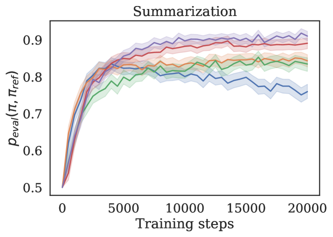
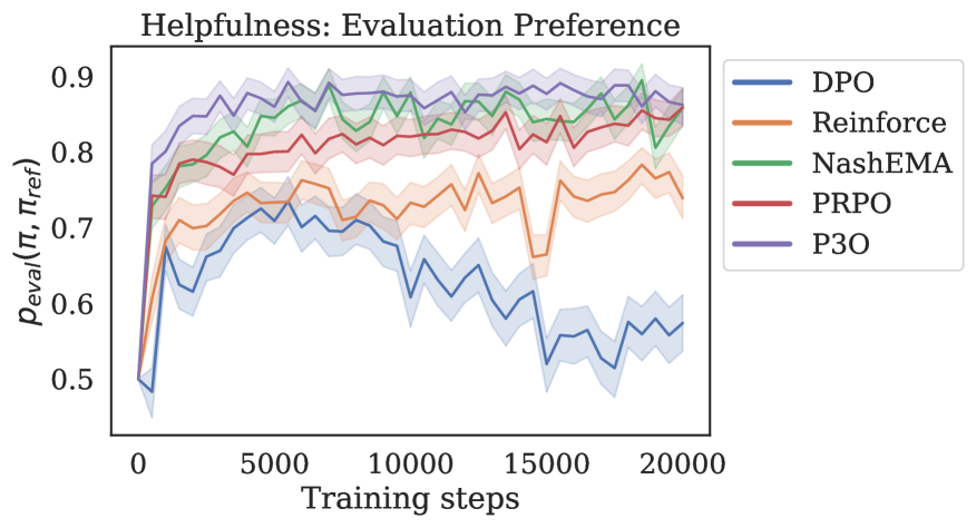
Figure 1: Comparison of our methods (P3O and PRPO) against standard approaches (REINFORCE and DPO) on summarization and “helpful assistant” tasks, showing the evaluation preference of a prompted Gemini evaluator, for generations of the policy over those of the reference policy. The hyperparameters of each method have been tuned to prevent reward hacking (best eval performance), which necessitates strong KL-regularization for DPO and REINFORCE. Our approaches, however, can avoid reward hacking by relying on pessimism instead of KL regularization (a blunt tool), and achieve consistently better performance as a result. We also compare to Nash-EMA (Munos et al., 2023), a natural baseline that also employs a preference model instead of a reward model, but without any pessimism. Like REINFORCE, the best Nash-EMA values still plateau to a lower performance on summarization. While it achieves similar win-rates over $\pi_{\mathrm{ref}}$ on helpfulness, it does so at the cost of much longer and idiosyncratic generations on average (see Figure 4). Shaded areas show $95\%$ CIs of the evaluation.

Motivated by these concerns, there is a growing literature on techniques to control this overoptimization behavior in more data-driven ways, such as by incorporating uncertainty in the predictions of the underlying reward model with explicit reward ensembles (Eisenstein et al., 2024; Coste et al., 2023), or pessimistic reasoning (Fisch et al., 2024; Liu et al., 2024; Huang et al., 2024b; Cen et al., 2024), albeit with only modest success in standard settings. Similar to the related area of distributionally robust optimization (Bertsimas & Sim, 2004; Ben-Tal et al., 2013), a core part of the challenge is balancing sufficient reward uncertainty and pessimism to prevent overoptimization, while still being able to learn effectively (Eisenstein et al., 2024; Fisch et al., 2024).

In contrast to the reward-based setting, much less work has studied the incorporation of uncertainty when using learned pairwise preference models in subsequent RL—with even fewer works devoted to understanding exactly what kinds of pessimistic possibilities due to uncertainty are useful to entertain, versus ignore. Pessimistic techniques for preference-based RL are particularly challenging, since many leading methods (Munos et al., 2023; Swamy et al., 2024; Calandriello et al., 2024) without pessimistic reasoning, critically leverage the symmetry of the min and max players in preference-based RL to develop efficient algorithms, but the introduction of additional pessimism breaks this symmetry. Additionally, the obvious pessimistic estimators studied theoretically in (Cui & Du, 2022; Ye et al., 2024) exhibit some pathologies when the offline dataset has systematic gaps in its coverage, arising from the non-transitivity of general preferences. These pathologies mean that despite using pessimism, we cannot easily compete with policies whose responses are adequately covered in the data—the typical benchmark for offline RL in reward-based settings.

In this work, we build on prior works in preference-based RLHF (Swamy et al., 2024; Munos et al., 2023), as well as offline learning in Markov games (Cui & Du, 2022), to obtain new robust objectives for incorporating a restricted form of uncertainty from finite preference datasets. Specifically, we make the following key contributions:

1. We identify problematic properties of prior pessimistic estimators (Cui & Du, 2022; Ye et al., 2024) in the absence of prohibitive coverage assumptions on the preference data sampling policy. We then develop a new restricted Nash formulation under which the learned policy is provably preferable to any other competitor policy that is restricted to choosing actions within the support of the preference data sampling policy, and show the theoretical benefits of this formulation.

2. We provide a practical algorithm, Pessimistic Preference-based Policy Optimization (P3O) for optimizing the resulting objective. We approximate the ideal theoretical objective with a variational upper bound, that yields a minimax game between a policy and a preference player, which we solve using gradient ascent-descent. The policy optimization is similar to prior works (Swamy et al., 2024; Munos et al., 2023) and the preference updates are adversarial to the current policy’s choices. For Bradley-Terry-Luce models with reward-based preferences, we also evaluate a simpler, reward-based variant of P3O (which we call PRPO) in our experiments.

3. Empirical evaluation on document summarization and training helpful assistants in Figure 1 shows P3O and PRPO reach a higher quality of responses quickly, and the quality does not degrade due to overoptimization from further training. This is contrast with standard RLHF methods (DPO (Rafailov et al., 2023), and REINFORCE (Willams, 1992; Ahmadian et al., 2024), which either exhibit significant overoptimization, or are limited in their ability to sufficiently optimize. The evaluations are performed using a prompted Gemini 1.5 Flash auto-evaluator (Gemini Team, 2024). Detailed analysis in Section 5 further shows that P3O and PRPO avoid qualitative reward hacking behavior of REINFORCE and DPO.

2 Background

We consider human alignment of a language model (LM) policy $\pi\in\Pi$, where $\Pi\subseteq\{{\mathcal{X}}\rightarrow\Delta({\mathcal{Y}})\}$, which generates for a context $x\in{\mathcal{X}}$, a response $y\sim\pi(\cdot|x)$ with $y\in{\mathcal{Y}}$. We assume that we are given access to a preference dataset, ${\mathcal{D}}$, consisting of tuples $(x,y_{w},y_{l})\in{\mathcal{X}}\times{\mathcal{Y}}\times{\mathcal{Y}}$ where for context $x$, the response $y_{w}$ is preferred over $y_{l}$ (as labeled by a human). We further assume access to a reference policy $\pi_{\mathrm{ref}}$, which may or may not match the original sampling policy for the preferred and dispreferred $(y_{w},y_{l})$ responses in ${\mathcal{D}}$. For brevity, we drop the context $x$ from the notation and work with a finite ${\mathcal{Y}}$ when there is no ambiguity.

Preferences are often modeled via a reward function under the Bradley-Terry-Luce (BTL) (Bradley & Terry, 1952; Luce, 2012) model (Christiano et al., 2017; Ouyang et al., 2022); however, in this paper, we make no such assumptions and work with both general pairwise preference functions as well as BTL preference functions based on pointwise rewards. In the following, we first set up the preference learning framework, and then discuss techniques to optimize policies with preference feedback, while also establishing the use of pessimism to handle uncertainties that may exist in the reward and preference functions.

Learning preferences from data.

We define the preference function $p:{\mathcal{Y}}\times{\mathcal{Y}}\rightarrow[0,1]$, such that $p(y_{1},y_{2})\doteq\Pr(y_{1}\succ y_{2})$ represents the probability of the generation $y_{1}$ being preferred over $y_{2}$ by a target user. Being a probability, the preference function satisfies: $p(y_{1},y_{2})=1-p(y_{2},y_{1})$. To obtain a preference model, we typically fine-tune a pretrained language model (LM) on ${\mathcal{D}}$ to produce the maximum likelihood estimate $p_{\mathrm{mle}}$ via the following objective:

$$\begin{split}\textstyle&p_{\mathrm{mle}}\in\mathop{\rm arg\,min}_{p}{\mathcal{L}}_{\mathrm{pref}}(p;{\mathcal{D}}),~~\mbox{where}~~\\ &{\mathcal{L}}_{\mathrm{pref}}(p;{\mathcal{D}})=-\mathbb{E}_{(y_{w},y_{l})\sim{\mathcal{D}}}\left[\mathop{\rm log}p\left(y_{w},y_{l}\right)\right].\end{split}$$ (1)

We overload the notation to say $p(\pi,\pi^{\prime})$, where $\pi,\pi^{\prime}\in\Pi$, to represent the expected preference for $\pi$ over $\pi^{\prime}$, given the preference function $p$, that is,

$$p(\pi,\pi^{\prime})=\mathbb{E}_{y\sim\pi,y^{\prime}\sim\pi^{\prime}}[p(y,y^{\prime})].$$

In the standard case of RLHF, the preference function is modeled using a reward function $r:{\mathcal{Y}}\rightarrow\mathbb{R}$, assuming an underlying BTL model $p_{\mathrm{BTL}}$, i.e.,

$$p_{\mathrm{BTL}}(y_{1},y_{2};r)\doteq\frac{\exp(r(y_{1}))}{\exp(r(y_{1}))+\exp(r(y_{2}))}.$$ (2)

Note that the set of BTL models is a strict subset of the general pairwise preference models. We also overload the notation $p_{\mathrm{BTL}}(r)$ to denote the BTL preference model that is induced by reward function $r$.

Preference-based policy optimization.

To optimize general preferences without making a BTL modeling assumption, following Munos et al. (2023) and Swamy et al. (2024), we formulate a preference game $J_{\mathrm{P}}(\pi,\pi^{\prime},p)$ between a pair of competing policies $\pi$ and $\pi^{\prime}$, with preference function $p$, a reference policy $\pi_{\mathrm{ref}}$, and a regularization parameter $\beta>0$, as

$$J_{\mathrm{P}}(\pi,\pi^{\prime},p)\doteq p(\pi,\pi^{\prime})-\beta{\mathrm{KL}}\left(\pi\|\pi_{\mathrm{ref}}\right)+\beta{\mathrm{KL}}\left(\pi^{\prime}\|\pi_{\mathrm{ref}}\right),$$

where ${\mathrm{KL}}\left(\pi\|\pi_{\mathrm{ref}}\right)\doteq\mathbb{E}_{y\sim\pi}\left[\mathop{\rm log}\tfrac{\pi(y)}{\pi_{\mathrm{ref}}(y)}\right]$. For the preference objective $J_{\mathrm{P}}$, the $\pi$ and $\pi^{\prime}$ players optimize their corresponding $\max$-$\min$ and $\min$-$\max$ objectives, i.e.,

$$\begin{split}&\pi_{\mathrm{nash}}\in\mathop{\rm arg\,max}_{\pi\in\Pi}\min_{\pi^{\prime}\in\Pi}J_{\mathrm{P}}(\pi,\pi^{\prime},p_{\mathrm{mle}}),\\ &\pi_{\mathrm{nash}}^{\prime}\in\mathop{\rm arg\,min}_{\pi^{\prime}\in\Pi}\max_{\pi\in\Pi}J_{\mathrm{P}}(\pi,\pi^{\prime},p_{\mathrm{mle}}).\end{split}$$ (3)

Here, due to the symmetry of the game, a Nash equilibrium exists at the same policy, i.e., $\pi_{\mathrm{nash}}=\pi_{\mathrm{nash}}^{\prime}$, and the objective can be simplified to optimizing a single-player game—termed Self-play Preference Optimization (SPO) in Swamy et al. (2024).

Alternatively, in the standard reward-based setup, given a reward function $r$, the corresponding objective for reward optimization becomes $J_{\mathrm{R}}(\pi,r)$, which is defined as:

$$J_{\mathrm{R}}(\pi,r)\doteq\mathbb{E}_{y\sim\pi}[r(y)]-\beta{\mathrm{KL}}\left(\pi\|\pi_{\mathrm{ref}}\right).$$ (4)

As described earlier, typical reward-based RLHF settings make use of a learned reward $r_{\mathrm{mle}}$ obtained by optimizing (1) for $p_{\mathrm{BTL}}$ in (2), and fine-tune the policy to maximize the expected pointwise reward, i.e.,

$$\pi_{\mathrm{rlhf}}\in\mathop{\rm arg\,max}_{\pi\in\Pi}J_{\mathrm{R}}(\pi,r_{\mathrm{mle}}),$$ (5)

$$~~\mbox{where}~~r_{\mathrm{mle}}\in\mathop{\rm arg\,min}_{r}{\mathcal{L}}_{\mathrm{pref}}\Big{(}p_{\mathrm{BTL}}(r);{\mathcal{D}}\Big{)}.$$

Pessimism in preference-based policy optimization.

It is a well-understood issue in preference optimization and RLHF that optimizing $J_{\mathrm{P}}(\cdot,\cdot,p_{\mathrm{mle}})$ and $J_{\mathrm{R}}(\cdot,r_{\mathrm{mle}})$ can lead to over-optimization of the corresponding preference and reward functions (Gao et al., 2023; Eisenstein et al., 2024). This behavior arises because $p_{\mathrm{mle}}$ (resp. $r_{\mathrm{mle}}$) has large inaccuracies and/or uncertainties in its predictions outside the support of ${\mathcal{D}}$, and the policy optimization to maximize the preference (resp. reward), can exploit the such regions with spuriously high scores under $p_{\mathrm{mle}}$ (resp. $r_{\mathrm{mle}}$), resulting in a shift in the distribution of outputs generated by the learned policies ($\pi_{\mathrm{nash}}$ and $\pi_{\mathrm{rlhf}}$). Colloquially, this phenomenon is often termed “reward hacking” or “preference hacking”. Pessimism in both the reward setting (Eisenstein et al., 2024; Liu et al., 2024; Fisch et al., 2024; Cen et al., 2024) and the preference setting (Ye et al., 2024) has been proposed as a way to remedy these issues.

Pessimism in the reward setting leads to a $\max$-$\min$ objective, $\pi_{\mathrm{p}\textrm{{-}}\mathrm{rlhf}}\in\mathop{\rm arg\,max}_{\pi}\min_{r\in{\mathcal{R}}}J_{\mathrm{R}}(\pi,r)$ where ${\mathcal{R}}$ is an uncertainty set of reward functions, that is, all reward functions that are consistent with the dataset. Liu et al. (2024) and Fisch et al. (2024) show that for certain choices of ${\mathcal{R}}$, this game can be solved without actually maintaining the set ${\mathcal{R}}$ and performing the inner optimization in closed form. In the following section, we extend this to the preference setting (again, which includes reward-based BTL preferences), while also analyzing what forms of pessimism are most appropriate for learning reasonable optimal policies under uncertainty.

3 Pessimistic Preference-based RL

We now define a natural extension of the pessimistic reward-based objective to the case of preferences, and study its improvements and generalizations. Implementation issues in developing an efficient algorithm are deferred to §4.

A pessimistic Nash solution.

In preference-based RL, a pessimistic counterpart of the Nash solution in (3) can be naturally formulated as

$$\pi_{\mathrm{p}\textrm{{-}}\mathrm{nash}} \in\mathop{\rm arg\,max}_{\pi}\min_{\pi^{\prime}}\min_{p\in{\mathcal{P}}}J_{\mathrm{P}}(\pi,\pi^{\prime},p)$$ (6)

where ${\mathcal{P}}\subseteq\{\ {\mathcal{Y}}\times{\mathcal{Y}}\to[0,1]\}$ defines an uncertainty set over preference functions. In particular we consider the set ${\mathcal{P}}({\mathcal{D}},c)\subset\{{\mathcal{Y}}\times{\mathcal{Y}}\to[0,1]\}$, for $c\geq 0$, which is defined as:

$${\mathcal{P}}({\mathcal{D}},c)\doteq\{p:{\mathcal{L}}_{\mathrm{pref}}(p;{\mathcal{D}})\leq{\mathcal{L}}_{\mathrm{pref}}(p_{\mathrm{mle}};{\mathcal{D}})+c\},$$ (7)

and choose ${\mathcal{P}}\doteq{\mathcal{P}}({\mathcal{D}},c^{\prime})$ for a value of $c^{\prime}$, such that $p^{\star}\in{\mathcal{P}}({\mathcal{D}},c^{\prime})$. This formulation has been studied previously for certain choices of ${\mathcal{P}}$ in the tabular (Cui & Du, 2022) and function approximation setting (Ye et al., 2024; Huang et al., 2024a). These works prove that the solution $\pi_{\mathrm{p}\textrm{{-}}\mathrm{nash}}$ converges to the optimal policy if and only if a condition called unilateral coverage holds, which requires that we can compare $\pi_{\mathrm{p}\textrm{{-}}\mathrm{nash}}$ with any response $y$, within the coverage of the sampling policy $\pi_{\mathrm{data}}$. That is, $p(\pi_{\mathrm{p}\textrm{{-}}\mathrm{nash}},y)$ lies within a small interval as we vary $p\in{\mathcal{P}}$, for all $y$. This approach has not been empirically evaluated in prior works, as the optimization problem is very challenging with no obvious practical strategies. Before discussing these algorithmic challenges, we will first explore the practical implications of the unilateral coverage requirement.

The implications of an unconstrained min player.

Consider an illustrative example in Figure 2 which is emblematic of typical RLHF scenarios. There is no context and ${\mathcal{Y}}=\{y_{1},y_{2},y_{3}\}$ and suppose further that we have that $p(y_{1},y_{2})=1$ for all $p\in{\mathcal{P}}$, so we are fully certain about this preference. But we never observe any comparisons involving $y_{3}$ in our preference data $(\pi_{\mathrm{data}}(y_{3})=0)$, and hence the set ${\mathcal{P}}$ allows all values $p(y,y_{3})\in[0,1]$ for $y\neq y_{3}$. To highlight the limitations of pessimism in preference optimization, we consider the problem in absence of regularization, i.e., $\beta=0$. Then, as illustrated in Figure 2 (Left) and proven in Appendix B, the pessimistic Nash policy $\pi_{\mathrm{p}\textrm{{-}}\mathrm{nash}}$ satisfies $\pi_{\mathrm{p}\textrm{{-}}\mathrm{nash}}(y_{3})=0.5$. That is, the policy takes an action completely out of the support of the sampled dataset w.p. $0.5$, where the ground-truth preferences can take completely arbitrary values. Intuitively, this happens because the pessimistic policy has to account for either possibility that $y_{1}$ is much better than $y_{3}$, or vice versa, since the set ${\mathcal{P}}$ is completely uncertain about the preference between $y_{3}$ and $y_{1}$. Indeed, in most practical applications, many possible $y$’s will not be covered in the dataset, even distributionally, and it appears undesirable that the optimal policy obtained by pessimism will then predominantly generate such outputs.

This example highlights a key distinction between pessimism with rewards versus pessimism with preferences. When using pessimism with rewards, outputs which are not covered in the data tend to get a low score, and a reward-maximizing policy naturally avoids such outputs. But in preference-based learning, the min player $\pi^{\prime}$ can choose any output which is not observed in the preference data, and pessimism over preferences means that the max player looses to this action in the worst case—forcing the max player to put probability over such an uncovered output as well. We now propose a remedy for this issue.

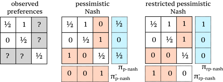
Figure 2: An illustration of the problematic example for pessimistic preference optimization with unrestricted opponents. We assume that $\{y_{1},y_{2}\}$ are well-sampled in the preference data, whereas $y_{3}$ is not—resulting in certain preferences for $y_{1}$ vs. $y_{2}$, but completely uncertain preferences for $y_{3}$ vs. others (Left). The $3\times 3$ matrices above are then the optimized pessimistic preference matrices for $\{y_{1},y_{2},y_{3}\}$, with the $3d$ vectors the optimized competing policies. Specifically, shaded entries represent optimizable variables, and the values in each of the blue and red shaded entries are the solutions for the max ($\mathop{\rm arg\,max}_{\pi}$) and min player ($\mathop{\rm arg\,min}_{\pi^{\prime}}$ and $\mathop{\rm arg\,min}_{p\in{\mathcal{P}}}$), resp., see (6). Middle: when the opponent $\pi^{\prime}$ is unrestricted, the optimal policy $\pi_{\mathrm{p}\textrm{{-}}\mathrm{nash}}$ must hedge and put significant support on $y_{3}$. Right: restricting the support of $\pi^{\prime}$ to the support of the preference-data (i.e., $\{y_{1},y_{2}\}$), avoids this issue, and yields a more reasonable optimal policy $\pi_{\mathrm{rp}\textrm{{-}}\mathrm{nash}}$.

Restricted pessimistic Nash with a constrained min player.

Given the example from Figure 2, an intuitive response is to consider a Nash strategy where the support for the opponent policy $\pi^{\prime}$ is restricted to actions which are well-sampled in the preference dataset. For tabular scenarios, where we have no contexts and a finite ${\mathcal{Y}}$, with all possible policies in the class $\Pi$, such a restriction can be carried out by explicitly constraining the support of the min-player in the pessimistic objective (6). However, this does not generalize to more practical scenarios with parametric policies over a large output space. Instead, for such situations, we define a subset $\Pi(\pi_{\mathrm{data}},C)\subseteq\Pi$ to be a set of policies whose outputs are “well-covered” by the sampling policy $\pi_{\mathrm{data}}$, with $C$ denoting a coverage parameter that we define below.

Definition 3.1 (Covered policy set).

For a given sampling policy $\pi_{\mathrm{data}}\in\Pi$ and constant $C$, the covered policy set $\Pi(\pi_{\mathrm{data}},C)$ with respect to $\pi_{\mathrm{data}}$ is the set of policies such that $\forall\pi,\pi^{\prime}\in\Pi(\pi_{\mathrm{data}},C)$ and $\forall p_{1},p_{2}\in{\mathcal{P}}$,

$$\begin{split}&\mathbb{E}_{y\sim\pi,y^{\prime}\sim\pi^{\prime}}(p_{1}(y,y^{\prime})-p_{2}(y,y^{\prime}))^{2}\\ &\hskip 14.22636pt\leq C\cdot\mathbb{E}_{y,y^{\prime}\stackrel{{\scriptstyle\mathrm{i.i.d.}}}{{\sim}}\pi_{\mathrm{data}}}(p_{1}(y,y^{\prime})-p_{2}(y,y^{\prime}))^{2}.\end{split}$$ (8)

What covered policies are included in $\Pi(\pi_{\mathrm{data}},C)$? Clearly, $\pi_{\mathrm{data}}\in\Pi(\pi_{\mathrm{data}},C)$ when $C\geq 1$. We assume $C\geq 1$ in the sequel to ensure that this containment happens. We can also show (see Appendix C.2 for a short derivation) that $\Pi(\pi_{\mathrm{data}},C)$ includes the set of all policies with likelihood ratios with respect to $\pi_{\mathrm{data}}$ that are uniformly bounded by $\sqrt{C}$, that is, $\Pi_{\sqrt{C}}\subseteq\Pi(\pi_{\mathrm{data}},C)$, where $\Pi_{\sqrt{C}}=\{\pi\in\Pi~:~\|\pi/\pi_{\mathrm{data}}\|_{\infty}\leq\sqrt{C}\}$.

In fact, we further show in Appendix C.3 that when the preference functions are linear in a shared feature map, then this coverage condition is ensured whenever the cross-covariance matrices of $\pi$ and $\pi^{\prime}$ are sufficiently aligned with the covariance matrix of $\pi_{\mathrm{data}}$.

Perhaps most importantly, however, when defining the following restricted pessimistic Nash solution, $\pi_{\mathrm{rp}\textrm{{-}}\mathrm{nash}}$, using this notion of coverage, i.e.,

$$\pi_{\mathrm{rp}\textrm{{-}}\mathrm{nash}}\in\mathop{\rm arg\,max}_{\pi\in\Pi}\min_{\pi^{\prime}\in\Pi(\pi_{\mathrm{data}},C)}\min_{p\in{\mathcal{P}}}J_{\mathrm{P}}(\pi,\pi^{\prime},p),$$ (9)

we can give the following performance guarantee for $\pi_{\mathrm{rp}\textrm{{-}}\mathrm{nash}}$ under the ground-truth preference function $p^{\star}$ which generated the preference dataset ${\mathcal{D}}$ (which was then used to derive the set of plausible preference functions ${\mathcal{P}}$).

Lemma 3.2 (Preference guarantee for the restricted pessimistic Nash policy).

We denote the restricted pessimistic Nash policy by $\pi_{\mathrm{rp}\textrm{{-}}\mathrm{nash}}$ from (9), and let $p^{\star}$ be the ground-truth preference function underlying ${\mathcal{D}}$. Then we have that for any $\pi\in\Pi(\pi_{\mathrm{data}},C)$ with $C\geq 1$:

$$p^{\star}(\pi_{\mathrm{rp}\textrm{{-}}\mathrm{nash}},\pi)\geq\frac{1}{2}-2\sqrt{C\varepsilon},$$

where $\varepsilon$ is a bound on how much preference functions in ${\mathcal{P}}$ can disagree in total variation under $\pi_{\mathrm{data}}$: $\mathbb{E}_{(y,y^{\prime})\stackrel{{\scriptstyle\mathrm{i.i.d.}}}{{\sim}}\pi_{\mathrm{data}}}|p_{1}(y,y^{\prime})-p_{2}(y,y^{\prime})|\leq\varepsilon$, $\forall p_{1},p_{2}\in{\mathcal{P}}$.

Appendix C.1 restates Definition 3.1 and Lemma 3.2 with the context $x$ included, along with a proof. This result shows that the restricted pessimistic Nash policy is always preferred to all other covered policies in $\Pi(\pi_{\mathrm{data}},C)$ up to an error term. In comparison, the unrestricted pessimistic Nash solution from (6) does not satisfy this guarantee in general. To see this, consider the example in Figure 2, where the unrestricted pessimistic Nash policy $\pi_{\mathrm{p}\textrm{{-}}\mathrm{nash}}=[1/2,0,1/2]$ is dispreferred to the covered policy $\pi_{1}=[1,0,0]$ with probability $p^{\star}(\pi_{1},\pi_{\mathrm{p}\textrm{{-}}\mathrm{nash}})=1/2+\gamma/2$ when $p^{\star}(y_{1},y_{3})=\gamma$.

As this example suggests, the unrestricted pessimistic solution can be arbitrarily dispreferred, even to covered policies. Existing analyses by Cui & Du (2022) for the unrestricted version indeed do not apply to this example since $\pi_{\mathrm{data}}(y_{3})=0$ and, thus, the necessary unilateral coverage condition is violated (Cui & Du, 2022). In fact, no policy can satisfy unilateral coverage in this case, and we get a vacuous guarantee out of their analysis. The same is true for the relaxed coverage condition of Zhang et al. (2023, Appendix B), as it still applies to the unrestricted pessimistic solution.

In some sense, the contrast between our result from Lemma 3.2 and those of Cui & Du (2022) is analogous to the classical analysis of offline RL methods (see, e.g., Chen & Jiang (2019)) and pessimistic offline RL techniques (Xie et al., 2021). Without pessimism in offline RL, we end up with vacuous guarantees, while the pessimistic results allow a non-trivial sub-optimality bound against any policy well covered by the data collection policy. Similarly, the results of Cui & Du (2022) offer a strong guarantee when the data collection policy is sufficiently exploratory, but are rendered vacuous without this. In contrast, our analysis of the restricted Nash estimator offers an opportunistic guarantee, where we are able to adaptively compete with all policies which are well covered by $\pi_{\mathrm{data}}$. We note that these considerations are particularly pertinent when aligning LLMs with small preference datasets, where the output space is of long sequences over a large vocabulary, of which the alignment data typically only covers a tiny sliver, leaving no hope for unilateral coverage style assumptions to be satisfied.

4 P3O: An Efficient Implementation

 Hyperparameters: Mixing coefficient $\alpha$, regularization coefficient $\beta$, preference regularization coefficient $\lambda$, EMA parameter $\gamma$, learning rates $(\eta_{p},\eta_{\pi})$

 Initialize: $\bar{\pi}_{1}=\pi_{1}=\pi_{\mathrm{ref}}$, $p_{1}=p_{\mathrm{mle}}$

 for $t=1,2,\dots$ do

  Set $\pi_{\mathrm{mix}}^{\alpha}\propto\bar{\pi}^{1-\alpha}_{t}\pi_{\mathrm{data}}^{\alpha}$ as mix of $\pi_{\mathrm{ref}}$ and the exponential moving average $\bar{\pi}_{t}$ for restricted Nash.

  Approximate the current objective (14):

$$J_{\mathrm{P3O}(\alpha)}(\pi_{t},p_{t})\doteq p_{t}(\pi_{t},\pi_{\mathrm{mix}}^{\alpha}) -\beta{\mathrm{KL}}\left(\pi_{t}\|\pi_{\mathrm{ref}}\right)$$

$$-\lambda\mathrm{KL}_{\pi_{\mathrm{ref}}}\left(p_{\mathrm{mle}}\|p\right)$$

  Update $\pi_{t+1}\leftarrow\pi_{t}+\eta_{\pi}\frac{\partial J_{\mathrm{P3O}(\alpha)}(\pi,p_{t})}{\partial\pi}\bigg{|}_{\pi=\pi_{t}}$

  Update $p_{t+1}\leftarrow p_{t}-\eta_{p}\frac{\partial J_{\mathrm{P3O}(\alpha)}(\pi_{t},p)}{\partial p}\bigg{|}_{p=p_{t}}$

  Update $\bar{\pi}_{t+1}\leftarrow\gamma\pi_{t}+(1-\gamma)\bar{\pi}_{t}$

 end for

Algorithm 1 P3O ​($\alpha$)

We now develop an efficient algorithm, Pessimistic Preference-based Policy Optimization (P3O), that approximately solves the restricted pessimistic Nash formulation.

Approximating the restricted policy set.

A first obstacle to an efficient algorithm is that the definition $\Pi(\pi_{\mathrm{data}},C)$ is not amenable to easy implementation. However, in KL-regularized preference-based RLHF, there is a natural heuristic to approximate this restriction via an additional KL regularization term. Recall that the central goal of $\Pi(\pi_{\mathrm{data}},C)$ is to limit optimization to policies $\pi$ which generate responses that are in the coverage of the data generating policy $\pi_{\mathrm{data}}$. We encourage this through adding an additional penalty based on the KL divergence between $\pi^{\prime}$ and $\pi_{\mathrm{data}}$:

$$\max_{\pi}\min_{p\in{\mathcal{P}}}\min_{\pi^{\prime}}\;\;p(\pi,\pi^{\prime})-\beta{\mathrm{KL}}\left(\pi\|\pi_{\mathrm{ref}}\right)$$ (10)

$$\quad+(1-\alpha)\beta{\mathrm{KL}}\left(\pi^{\prime}\|\pi_{\mathrm{ref}}\right)+\alpha\beta{\mathrm{KL}}\left(\pi^{\prime}\|\pi_{\mathrm{data}}\right).$$

Note that $\pi^{\prime}$ is regularized with respect to both the reference policy $\pi_{\mathrm{ref}}$ and the sampling policy $\pi_{\mathrm{data}}$, where the added parameter $\alpha$ controls the relative strength of the contribution of $\pi_{\mathrm{ref}}$ versus $\pi_{\mathrm{data}}$. While going from a data-aware constraint in terms of $\Pi(\pi_{\mathrm{data}},C)$ to KL regularization is lossy, we note that this is for the $\min$ player $\pi^{\prime}$ and only affects the max player $\pi$ through the data-dependent $p$ term.

We use P3O ​($\alpha$) to denote this variant, with P3O being the shorthand for P3O ​(0). Using a closed-form solution to the inner KL-regularized problem for $\pi^{\prime}$, we next show how to obtain an equivalent, but greatly simplified, objective for $\pi$. First, we define the shorthand $\pi_{\mathrm{mix}}^{\alpha}(y;\pi_{1},\pi_{2})$ as:

$$\begin{split}\pi_{\mathrm{mix}}^{\alpha}(y;\pi_{1},\pi_{2})\propto\pi_{1}^{1-\alpha}(y)\pi_{2}^{\alpha}(y).\end{split}$$ (11)

Optimizing $\pi$ against an appropriate mixed distribution is then equivalent to solving for $\eqref{eq:restricted-objective}$, as we show below.

Lemma 4.1.

The optimization problem in (10) is equivalent to the following objective, assuming that the minimization over $\pi^{\prime}$ is over all possible policies:

$$\begin{split}\max_{\pi}\min_{p\in{\mathcal{P}}}&-\mathop{\rm log}\mathbb{E}_{y\sim\pi_{\mathrm{mix}}^{\alpha}(\pi_{\mathrm{ref}},\pi_{\mathrm{data}})}\left[e^{\frac{-p(\pi,y)}{\beta}}\right]\\ &\quad-\beta{\mathrm{KL}}\left(\pi\|\pi_{\mathrm{ref}}\right).\end{split}$$ (12)

We provide a proof of this equivalence in Appendix D. We also note that replacing $\pi_{\mathrm{mix}}^{\alpha}(\pi_{\mathrm{ref}},\pi_{\mathrm{data}})$ with $\pi_{\mathrm{ref}}$ (i.e., $\alpha=0$) gives an equivalent rewriting for the pessimistic Nash objective with no support restrictions, as given in (6).

Approximating the log-partition function.

The objective in Lemma 4.1 simplifies the inner minimization to only have one variable, but at the cost of changing the objective to have a more complicated log-partition function term. Consequently, we can no longer get unbiased stochastic gradients of the objective from a mini-batch of data, due to the non-linearity of the logarithm outside of the expectation.

To obtain a practical algorithm, we leverage ideas from variational inference (Jordan et al., 1999) to approximate the log-partition function. Doing so, we obtain the following result, which is proved in Appendix E.

Lemma 4.2.

For any choice of policies $\pi,\bar{\pi}\in\Pi$:

$$\min_{p\in{\mathcal{P}}}-\mathop{\rm log}\mathbb{E}_{y\sim\pi_{\mathrm{mix}}^{\alpha}(\pi_{\mathrm{ref}},\pi_{\mathrm{data}})}\left[e^{\frac{-p(\pi,y)}{\beta}}\right]$$

$$\hskip 21.33955pt\leq\min_{p\in{\mathcal{P}}}\mathbb{E}_{y\sim\pi_{\mathrm{mix}}^{\alpha}(\bar{\pi},\pi_{\mathrm{data}})}\left[\frac{p(\pi,y)}{\beta}\right]+\kappa,$$ (13)

where $\kappa$ is independent of $\pi$ and $p$.

Due to the direction of the inequality, Lemma 4.2 gives only an upper bound for our objective in Lemma 4.1, and therefore maximizing the two is not equivalent. Nevertheless, the approximate objective is tractable, and simply takes the form of optimizing preferences against some comparator $\bar{\pi}$ mixed with the sampling distribution. Furthermore, the approximate objective at any fixed value of $p$ is tight when $\bar{\pi}(y)^{1-\alpha}\propto\exp(-p(\pi,y)/\beta)$, which resembles the multiplicative weight updates observed in prior self-play algorithms (Swamy et al., 2024; Munos et al., 2023). Since the current preference function iterate $p_{t}$ is slowly moving during gradient descent, with this motivation in hand, we choose the competitor policy $\bar{\pi}$ to be an exponentially moving average of past policy iterates in our experiments, giving our algorithm a pessimistic self-play flavor.

Approximating the preference uncertainty set.

As a final step, we replace the constrained optimization over the preference uncertainty set ${\mathcal{P}}$ with an unconstrained optimization over all preference functions in some parametric family by adding an additional loss term $-{\mathcal{L}}_{\mathrm{pref}}(p;{\mathcal{D}})~$(Liu et al., 2024), corresponding to the Lagrangian form of the constraint defining ${\mathcal{P}}$. The objective function then becomes

$$\mathbb{E}_{y\sim\pi_{\mathrm{mix}}^{\alpha}(\bar{\pi},\pi_{\mathrm{data}})}[p(\pi,y)]-\beta{\mathrm{KL}}\left(\pi\|\pi_{\mathrm{ref}}\right)-\lambda{\mathcal{L}}_{\mathrm{pref}}(p;{\mathcal{D}}),$$

where we rescaled the objective to absorb the $1/\beta$ on $p$ into the corresponding hyper-parameters of the KL and likelihood loss components (i.e., $\beta,\lambda$). The above objective requires us to also load the preference dataset ${\mathcal{D}}$ while trying to learn the policy, which can be somewhat inconvenient. To circumvent this issue, however, we can instead simply regularize the preference model to stay close to $p_{\mathrm{mle}}$, i.e.,

$$J_{\mathrm{P3O}(\alpha)}(\pi,p)\doteq ~p\Big{(}\pi,\pi_{\mathrm{mix}}^{\alpha}(\bar{\pi},\pi_{\mathrm{data}})\Big{)}$$ (14)

$$-\beta{\mathrm{KL}}\left(\pi\|\pi_{\mathrm{ref}}\right)-\lambda\mathrm{KL}_{\pi_{\mathrm{data}}}\left(p_{\mathrm{mle}}\|p\right),$$

where $\mathrm{KL}_{\pi_{\mathrm{data}}}\left(p_{\mathrm{mle}}\|p\right)$ is defined as

$$\mathbb{E}_{y,y^{\prime}\stackrel{{\scriptstyle\mathrm{i.i.d.}}}{{\sim}}\pi_{\mathrm{data}}\!\!}\left[{\mathrm{KL}}\left(p_{\mathrm{mle}}(y,y^{\prime})\|p(y,y^{\prime})\right)\right].$$

If the MLE solution $p_{\mathrm{mle}}$ is a good approximation to the true preferences $p^{\star}$ on $y,y^{\prime}\stackrel{{\scriptstyle\mathrm{i.i.d.}}}{{\sim}}\pi_{\mathrm{data}}$, then this KL divergence provides a good approximation to the likelihood-based version. The resulting algorithm is shown in Algorithm 1.

Having introduced P3O, which handles general preferences, we can extend it to the special case where preferences are parameterized by a reward function under the BTL model. In this setting, we replace the general preference function $p$ with $p_{\mathrm{BTL}}(r)$ in (14), resulting in the following objective:

$$J_{\mathrm{PRPO}(\alpha)}(\pi,r)\doteq p_{\mathrm{BTL}}\Big{(}\pi,\pi_{\mathrm{mix}}^{\alpha}(\bar{\pi},\pi_{\mathrm{data}}){;}r\Big{)}$$ (15)

$$\quad-\beta{\mathrm{KL}}\left(\pi\|\pi_{\mathrm{ref}}\right)-\lambda\mathrm{KL}_{\pi_{\mathrm{data}}}\left(p_{\mathrm{BTL}}(r_{\mathrm{mle}})\|p_{\mathrm{BTL}}(r)\right).$$

We refer to the algorithm that optimizes (15) as Pessimistic Reward-based Policy Optimization (PRPO). Appendix F provides the pseudo code and further discussion on PRPO.

5 Experimental Results

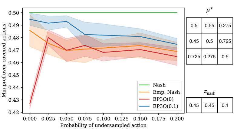
Figure 3: Tabular experiments: Comparison of the different objectives with an explicit search over the main policy, opponent policy, and version space. The $X$-axis shows the probability assigned to the under-sampled output ($y_{3}$), from $0.0\rightarrow 0.2$. The $Y$-axis indicates the minimum preference of the policy found over all covered actions (higher is better). We also show the ground-truth preference matrix $p^{\star}$ (top-right) and the corresponding $\pi_{\mathrm{nash}}$ (bottom-right). Results are averaged over 10 random seeds, shaded areas represent $\pm 2\times$ std error. EP3O(0.1) corresponding to the restricted Nash formulation consistently does well, particularly when the sampling rate of $y_{3}$ is very low (left part of plot).

In this section, we illustrate through multiple experiments the effectiveness of the P3O approach. We begin with evaluating the solution $\pi_{\mathrm{rp}\textrm{{-}}\mathrm{nash}}$ to the exact objective (12) by performing a brute force search over all the variables in a small tabular environment to understand how the objective performs for simple games. Next, we perform experiments on summarization and helpfulness tasks using the approximate objective $J_{\mathrm{P3O}(\alpha)}$ (14) to demonstrate its effectiveness.

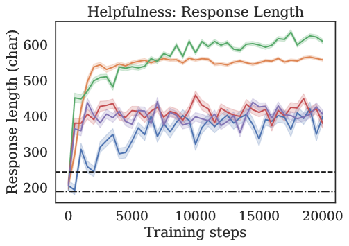
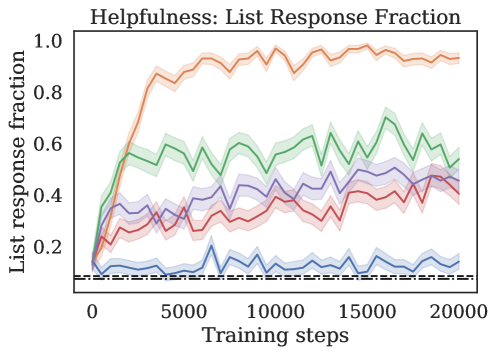
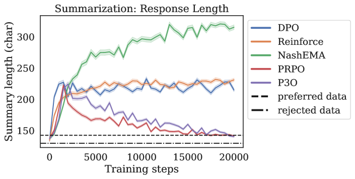
Figure 4: Qualitative results for the helpfulness and summarization tasks: On helpfulness, both response length and list formats are common reward hacks (Eisenstein et al., 2024). While policies do generate longer responses than the responses in $\pi_{\mathrm{data}}$, both REINFORCE and Nash-EMA converge on generations that are $\approx 40-50\%$ longer than those of P3O and PRPO (left). Similarly, REINFORCE degenerates into producing responses that are nearly all formatted as lists (with Nash-EMA at over $50\%$), while P3O and PRPO stay closer to $\pi_{\mathrm{data}}$ (middle). On summarization, DPO, REINFORCE, and Nash-EMA all show clear signs of length hacking—also a pervasive issue on this task (Eisenstein et al., 2024; Singhal et al., 2023; Park et al., 2024). In contrast, both PRPO and P3O converge to the average length of preferred responses in $\pi_{\mathrm{data}}$, all while also achieving the highest win-rates (right).

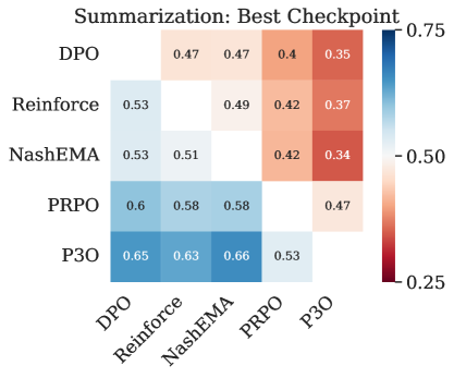
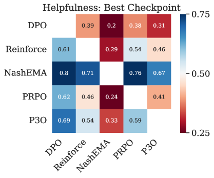
Figure 5: Confusion matrix showing the pairwise evaluation across the different methods, for each method’s best checkpoint selected in terms of preferences over the reference policy. In head-to-head comparisons, P3O and PRPO outperform baselines, except Nash-EMA on helpfulness, where the Gemini 1.5 Flash evaluation preference aligns with the preference model used for training—favoring the verbose, list-heavy outputs of Nash-EMA (and REINFORCE, to a lesser degree). However, when looking for both helpful and concise responses, P3O and PRPO win rates increase dramatically against Nash-EMA (see Figure 14 in the appendix), demonstrating their robustness.

Tabular experiments.

We first conduct experiments in a controlled, tabular setting with three possible outputs $y\in\{y_{1},y_{2},y_{3}\}$, and a ground-truth preference matrix $p^{\star}$. We vary the probability of sampling $y_{3}$ from $0.0$ to $0.2$, distributing the remaining probability equally among $(y_{1},y_{2})$. Thus, $y_{3}$ is consistently the under-sampled output. We conduct experiments with varying Nash strategies, including cases where $y_{3}$ is preferred, as well as dispreferred over the other two actions. Complete details about the experimental setup and search procedure are provided in Appendix G.

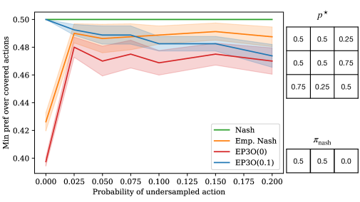
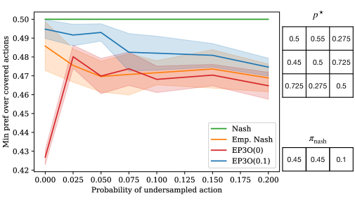
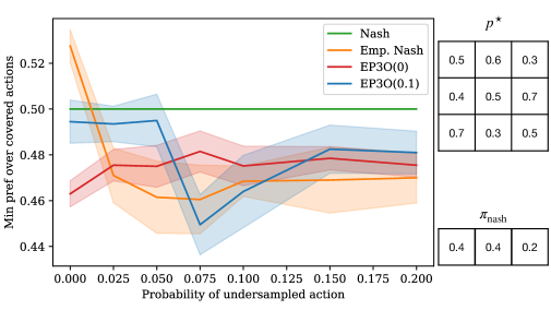
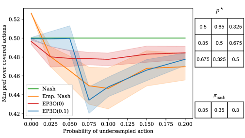
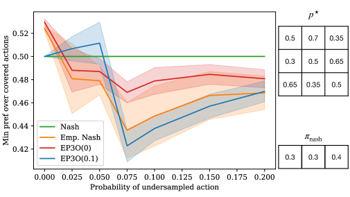
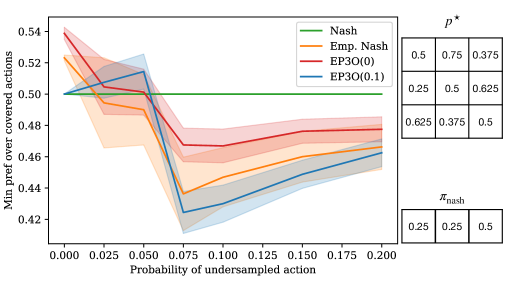
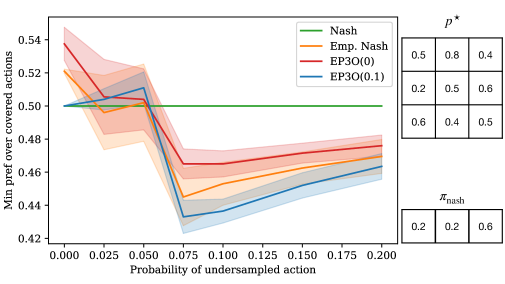
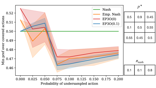
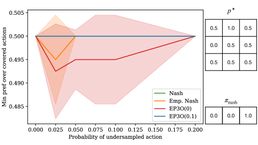
Figure 6: Tabular experiments (Continued from Figure 3) Comparison of the different objective functions with an explicit search over the main policy, opponent policy, and version space. The $X$-axis shows the probability assigned to the under-sampled output ($y_{3}$), from $0.0\rightarrow 0.2$. The $Y$-axis indicates the minimum preference of the policy found over all covered actions (higher is better). Each plot corresponds to a differernt $p^{\star}$ setting. Each figure also shows the ground-truth preference matrix $p^{\star}$ (on the top-right) and the corresponding $\pi_{\mathrm{nash}}$ (bottom-right) to each plot. Results are averaged over 10 random seeds, shaded areas represent $\pm 2\times$ standard error. EP3O(0.1) corresponding to the restricted Nash formulation consistently does well, particularly when the undersampled output is dispreferred and its sampling rate is very low (left part of plot).

Figure 3 illustrates a case in which the under-sampled action is dispreferred ($\pi_{\mathrm{nash}}(y_{3})=0.1$). We compare Exact P3O ​(0.1) (EP3O ​(0.1)), EP3O ​(0), as defined in Eq. (12), and the non-pessimistic Nash policy obtained from $p_{\mathrm{mle}}$. Additional scenarios, including ones where the under-sampled action is genuinely preferred, appear in Figure 6 (see Appendix G). Notably, EP3O ​(0.1) serves as a robust default choice: when the under-sampled action is truly dispreferred (particularly under extremely low sampling), the restricted pessimism in EP3O ​(0.1) prevents the policy from overcommitting to an insufficiently explored but suboptimal action. Conversely, if the under-sampled action is actually favored under the true $\pi_{\mathrm{nash}}$, even a small amount of data may guide non-pessimistic methods to weight that action correctly—potentially yielding strong performance. Since we typically lack ground-truth preferences, EP3O ​(0.1) offers a “safe-default” strategy.

Task 1: Summarization.

To demonstrate the effectiveness of our approach in mitigating preference hacking, we compare it against existing preference optimization methods on the popular TL;DR summarization task (Völske et al., 2017; Stiennon et al., 2020). Following prior studies on reward hacking for TL;DR (Eisenstein et al., 2024), we train an MLE preference model $p_{\mathrm{mle}}$ as well as MLE reward model $r_{\mathrm{mle}}$ by fine-tuning a T5 XL (3B) model (Raffel et al., 2020; Roberts et al., 2023) on the preference dataset. The initial policy $\pi_{\mathrm{ref}}$ is obtained by supervised fine-tuning a T5 large model (770M) on the human reference summaries in TL;DR. Choosing a larger preference model than the policy is a commonly employed strategy for mitigating hacking (Eisenstein et al., 2024). We initialize the training preference model $p_{1}\doteq p_{\mathrm{mle}}$ in case of P3O, and $r_{1}\doteq r_{\mathrm{mle}}$ in case of PRPO.

Task 2: Helpfulness.

We also test our method at larger scales on the Anthropic Helpfulness task (Bai et al., 2022) using 8B PaLM-based (Anil et al., 2023) policy, reward, and preference models. The helpfulness tasks consists of dialogues between humans and an automated assistant. The goal is to complete the next turn of the assistant by producing an engaging and helpful response. Like before, we obtain MLE preference and reward models by fine-tuning a pre-trained PaLM model on the preference data. These checkpoints are also used to initialize the preference and reward models for P3O and PRPO. The initial policy $\pi_{\mathrm{ref}}$ is obtained from an instruction-tuned PaLM model.

We compare P3O and PRPO against existing popular non-pessimistic RLHF methods, DPO (Rafailov et al., 2023) and REINFORCE (Willams, 1992) (which has been shown to outperform PPO (Ahmadian et al., 2024)), as well as the preference-model-based method Nash-EMA (Munos et al., 2023) (which is also non-pessimistic). We also compare to PDPO (Fisch et al., 2024), a pessimistic, offline variant of DPO, in Appendix H. We set $\alpha=0$ for our methods, as in these experiments $\pi_{\mathrm{ref}}$ and $\pi_{\mathrm{data}}$ are similar, and hence $\alpha$ does not influence the behavior of P3O.

All policies are evaluated using preferences assigned by Gemini 1.5 Flash (Gemini Team, 2024).

Results.

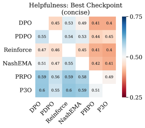
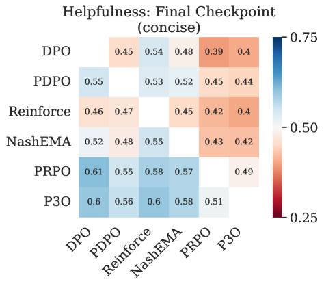
Figure 14: Confusion matrix showing the pairwise evaluation across the different methods when using an evaluation that emphasizes both helpful and concise prompts for the helpfulness tasks. See the “Helpfulness Concise Evaluation Prompt” shown below. This results in much poorer performance for the length-hacked REINFORCE and Nash-EMA models, whereas the non-length-hacked pessimistic methods P3O and PRPO still perform very well—demonstrating the better robustness pessimism affords to train/eval preference mismatches.

Figure 1 shows that the non-pessimistic baselines plateau at a lower overall performance level in general, with DPO even degrading substantially with prolonged training. In contrast, both P3O and PRPO achieve a significantly higher preference over $\pi_{\mathrm{ref}}$, surpassing the baselines (a result which is further supported by the confusion matrices in Figure 5). The lone exception is Nash-EMA on helpfulness, which performs very strongly according to our Gemini 1.5 evaluator—a result that happens to be helped by the alignment of the Gemini 1.5 evaluation preference with Nash-EMA’s generally longer responses. Under an evaluation that emphasizes both helpful and concise responses, P3O and PRPO are significantly better (Figure 14). Notably, the preference-based P3O outperforms the reward-based PRPO, indicating the advantage of general preference models.

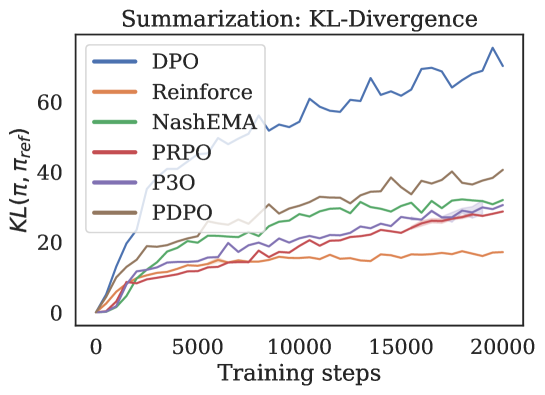
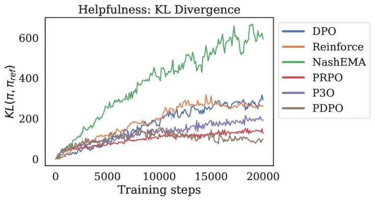
Figure 12: KL Divergence. The horizontal axis represents the number of training steps, while the vertical axis indicates the KL divergence of the learned policy from $\pi_{\mathrm{ref}}$. Results are presented for both summarization (left) and helpfulness (right) tasks. Pessimistic methods consistently demonstrate lower KL divergence (together with strong evaluation win-rates, per Figure 1) compared to RLHF approaches, despite utilizing significantly smaller values of $\beta$.

Figure 4 also illustrates how pessimism results in qualitatively different outputs by helping to avoid some of the common “hacking” behaviors related to length and style across different tasks that have been well-reported in the literature (Eisenstein et al., 2024; Singhal et al., 2023; Park et al., 2024). In particular, a typical form of reward hacking in summarization is “length hacking”, where policies inflate their rewards by producing overly verbose responses. We observe that non-pessimistic methods generate summaries significantly longer than those in the original dataset. In contrast, P3O and PRPO converge to summary lengths that are more consistent with $\pi_{\mathrm{ref}}$. Interestingly, while REINFORCE exhibits length hacking whereas P3O and PRPO do not, in Figure 12 (left) we see that REINFORCE actually maintains a lower KL divergence from $\pi_{\mathrm{ref}}$ compared to P3O and PRPO. This suggests that P3O and PRPO are learning policies that are substantially distributionally distant from $\pi_{\mathrm{ref}}$, but along quality dimensions that are distinct from simply length (and that result in higher perceived quality in our evaluations in Figure 1). Additionally, for helpfulness, we observe that REINFORCE tends to format nearly all responses as lists, much higher than the prevalence of lists in the preference data (Figure 4, middle), an artifact not shared by the responses of P3O or PRPO. We also observe a significant inflation in response lengths for both REINFORCE and Nash-EMA in helpfulness, converging to nearly 1.5x the response lengths for P3O and PRPO. In Appendix H, we present further results on the training dynamics which indicate a steadily improved objective for all the methods, even when the eval performance is non-monotonic. We also show some cherry-picked responses for both summarization and helpfulness tasks to illustrate the stylistic differences in their responses. We refer the reader to Appendix H for these and further details and results of our empirical evaluation.

6 Conclusion

Modern RLHF methods suffer from a significant tendency to overoptimize spurious preferences (or rewards) that are derived from faulty preference (or reward) models. In this work, we introduced pessimistic, preference-based RLHF objectives, which carefully balance uncertainty with effective learning. In particular, we theoretically analyzed the limitations of existing pessimistic estimators, and derive a novel formulation for a restricted, pessimistic Nash solution with provable advantages. Empirical results on multiple tasks and models demonstrate that our approach effectively resists overoptimization while outperforming standard RLHF baselines—highlighting the potential of pessimistic objectives for achieving robust language model alignment.

Impact Statement

This paper introduces new ideas to the active field of research on large language model post-training, which we hope will help facilitate the successful alignment of models to human preferences, as well as improve our understanding of current approaches—with the goal of ultimately supporting the development of capable and reliable AI systems that are easier, and more stable, to finetune.

Appendix A Extended Literature Review

Offline RL is primarily concerned with learning a policy from a fixed dataset, a problem that has attracted considerable attention. Many works focus on scenarios with sufficiently broad dataset coverage (Antos et al., 2007, 2008; Munos, 2003; Munos & Szepesvári, 2008; Farahmand et al., 2010; Chen & Jiang, 2019; Xie & Jiang, 2020), though such assumptions tend to be overly restrictive and seldom hold in real-world situations. Consequently, recent research has shifted toward the more realistic setting of inadequate coverage (Wang et al., 2020), aiming to learn a “best effort” policy (Liu et al., 2020). Two major strategies have emerged to handle poor coverage: behavior policy regularization (Fujimoto et al., 2019; Laroche et al., 2019; Kumar et al., 2019; Wu et al., 2019; Jaques et al., 2019; Kostrikov et al., 2021; Xiao et al., 2023) and pessimism in the face of uncertainty (Kumar et al., 2020; Liu et al., 2020; Kidambi et al., 2020; Yu et al., 2020; Buckman et al., 2020; Jin et al., 2021; Zanette et al., 2021; Xie et al., 2021; Cheng et al., 2022; Zhang et al., 2024; Koppel et al., 2024). In limited-data regimes, pessimism has been shown to provide strong theoretical guarantees for the resulting policy (Buckman et al., 2020; Jin et al., 2021), achieving min-max optimality in linear MDPs. Moreover, it has been successfully incorporated into both linear (Zanette et al., 2021) and deep RL (DRL) settings (Xie et al., 2021; Cheng et al., 2022).

Behavior policy regularization has also been explored in language models (Jaques et al., 2019), alongside standard RLHF approaches that commonly regularize to a reference policy (Stiennon et al., 2020). When the reward function is learned from limited data, inaccuracies naturally arise, mirroring the challenge in value-based offline RL where value estimates become unreliable in underrepresented state-action regions. Pessimism thus serves as a compelling remedy and has recently been investigated in the standard reward-based setting. Concurrently, several works (Fisch et al., 2024; Liu et al., 2024; Cen et al., 2024) have proposed offline methods that learn policies against an adversarial reward function, leveraging the DPO simplification (Rafailov et al., 2023) to avoid full-fledged adversarial training; among these, Cen et al. (2024) also introduces an online variant. Eisenstein et al. (2024) explores reward uncertainty through an ensemble of reward models, showing that ensemble aggregation helps mitigate reward hacking, though it does not fully resolve over-optimization risks.

On the preference-learning front, recent work has relaxed the BTL assumption, either by bypassing the need for a separate preference model (Azar et al., 2023; Tang et al., 2024) or adopting self-play approaches (Munos et al., 2023; Swamy et al., 2024; Calandriello et al., 2024; Ye et al., 2024). Ye et al. (2024) introduces a pessimistic preference objective with unrestricted Nash, and empirically evaluates an uncertainty based exploration method for the preference optimization. However, the role of pessimism in the more general preference-learning setting remains largely unexplored.

Appendix B Optimal Solution of the Example in Figure 2

Let $\pi_{i}=\pi(y_{i})$ and $p_{23}=p(y_{2},y_{3})$ and $p_{13}=p(y_{1},y_{3})$. Then we can write the objective in this example as

$$V^{\star}=\max_{\pi}\min_{\pi^{\prime}}\min_{p\in{\mathcal{P}}}J(\pi,\pi^{\prime},p)$$

$$\textrm{ where }J(\pi,\pi^{\prime},p)=p(\pi,\pi^{\prime})=\big{(} \,\,0.5\pi_{1}\pi^{\prime}_{1}+1\cdot\pi_{1}\pi^{\prime}_{2}+p_{13}\pi_{1}\pi^{\prime}_{3}$$

$$+0\cdot\pi_{2}\pi^{\prime}_{1}+0.5\pi_{2}\pi^{\prime}_{2}+p_{23}\pi_{2}\pi^{\prime}_{3}$$

$$+(1-p_{13})\pi_{3}\pi^{\prime}_{1}+(1-p_{23})\pi_{3}\pi^{\prime}_{2}+0.5\pi_{3}\pi^{\prime}_{3}\big{)}.$$

Upper-bound on $V^{\star}$:

First note that for any $\pi$:

$$\min_{\pi^{\prime}}\min_{p\in{\mathcal{P}}}J(\pi,\pi^{\prime},p)\leq 0.5\pi_{3}\qquad\textrm{and}\qquad\min_{\pi^{\prime}}\min_{p\in{\mathcal{P}}}J(\pi,\pi^{\prime},p)\leq 0.5\pi_{1}.$$

The first inequality follows by considering the choice $p_{13}=p_{23}=1$, and the second inequality from considering the choice $\pi^{\prime}_{1}=1$ and $p_{13}=1$. Since both bounds hold simultaneously and $\pi_{1}+\pi_{3}\leq 1$, we can conclude that

$$V^{\star}\leq 0.25.$$

Lower-bound on $V^{\star}$:

Choosing $\pi_{1}=\pi_{3}=0.5$, we see that the objective value can be written as

$$J(\pi,\pi^{\prime},p)= \big{(}0.25\pi^{\prime}_{1}+0.5\pi^{\prime}_{2}+0.5p_{13}\pi^{\prime}_{3}$$

$$+0.5(1-p_{13})\pi^{\prime}_{1}+0.5(1-p_{23})\pi^{\prime}_{2}+0.25\pi^{\prime}_{3}\big{)}.$$

First we observe that the minimum of this quantity is always attained at $p_{23}=1$ and thus we can ignore the penultimate term. Consider now two cases:

• Case $\pi^{\prime}_{1}\leq\pi^{\prime}_{3}$: Then the coefficient of $p_{13}$ is non-negative and the minimum is attained at $p_{13}=0$. This allows us to simplify the expression further as

  $$\min_{\pi^{\prime}}\min_{p\in{\mathcal{P}}}J(\pi,\pi^{\prime},p) =\min_{\pi^{\prime}}0.25\pi^{\prime}_{1}+0.5\pi^{\prime}_{2}+0.5\pi^{\prime}_{1}+0.5\pi^{\prime}_{2}+0.25\pi^{\prime}_{3}$$

  $$=\min_{\pi^{\prime}}0.75\pi^{\prime}_{1}+\pi^{\prime}_{2}+0.25\pi^{\prime}_{3}$$

  $$=0.25$$

  where we choose $\pi^{\prime}_{3}=1$ in the last step.

• Case $\pi^{\prime}_{1}\geq\pi^{\prime}_{3}$: Then the coefficient of $p_{13}$ is non-positive and the minimum is attained at $p_{13}=1$. This gives

  $$\min_{\pi^{\prime}}\min_{p\in{\mathcal{P}}}J(\pi,\pi^{\prime},p) =\min_{\pi^{\prime}}0.25\pi^{\prime}_{1}+0.5\pi^{\prime}_{2}+0.5\pi^{\prime}_{3}+0.5\pi^{\prime}_{2}+0.25\pi^{\prime}_{3}$$

  $$=\min_{\pi^{\prime}}\min_{P\in{\mathcal{P}}}0.25\pi^{\prime}_{1}+\pi^{\prime}_{2}+0.75\pi^{\prime}_{3}$$

  $$=0.25$$

  where the optimal solution is to choose $\pi^{\prime}_{1}=1$.

Combining both cases, we can conclude that

$$V^{\star}\geq 0.25.$$

Optimal solution.

Combining both upper- and lower-bounds, we can conclude that $V^{\star}=0.25$ which is attained at $\pi_{1}=\pi_{3}=0.5$.

Appendix C Definition and Analysis of Restricted Nash Policy

C.1 Restatement and Proof of Lemma 3.2

We restate Definition 3.1 and Lemma 3.2 over here, but with conversation context ($x$) included in the equations for clarity, hence for this section we redefine ${\mathcal{P}}\subseteq\{{\mathcal{X}}\times{\mathcal{Y}}\times{\mathcal{Y}}\to[0,1]\}$. We also use $x\sim{\mathcal{D}}$ to denote a context $x$ sampled from the offline dataset.

Definition C.1 (Covered policy set).

For a given sampling policy $\pi_{\mathrm{data}}\in\Pi$ and constant $C$, the covered policy set $\Pi(\pi_{\mathrm{data}},C)$ with respect to $\pi_{\mathrm{data}}$ is the set of policies such that $\forall\pi,\pi^{\prime}\in\Pi(\pi_{\mathrm{data}},C)$ and $\forall p_{1},p_{2}\in{\mathcal{P}}$,

$$\begin{split}&\mathbb{E}_{x\sim{\mathcal{D}},y\sim\pi(\cdot|x),y^{\prime}\sim\pi^{\prime}(\cdot|x)}(p_{1}(x,y,y^{\prime})-p_{2}(x,y,y^{\prime}))^{2}\\ &\hskip 14.22636pt\leq C\cdot\mathbb{E}_{x\sim{\mathcal{D}},y,y^{\prime}\stackrel{{\scriptstyle\mathrm{i.i.d.}}}{{\sim}}\pi_{\mathrm{data}}(\cdot|x)}(p_{1}(x,y,y^{\prime})-p_{2}(x,y,y^{\prime}))^{2}.\end{split}$$ (16)

Lemma C.2 (Preference guarantee for the restricted pessimistic Nash policy).

We denote the restricted pessimistic Nash policy by $\pi_{\mathrm{rp}\textrm{{-}}\mathrm{nash}}$ from Eq. (9), and let $p^{\star}$ be the ground-truth preference function underlying ${\mathcal{D}}$. Then we have that for any $\pi\in\Pi(\pi_{\mathrm{data}},C)$ with $C\geq 1$:

$$p^{\star}(\pi_{\mathrm{rp}\textrm{{-}}\mathrm{nash}},\pi)\geq\frac{1}{2}-2\sqrt{C\varepsilon},$$

where $\varepsilon$ is a bound on how much preference functions in ${\mathcal{P}}$ can disagree in total variation under $\pi_{\mathrm{data}}$: $\mathbb{E}_{x\sim{\mathcal{D}},(y,y^{\prime})\stackrel{{\scriptstyle\mathrm{i.i.d.}}}{{\sim}}\pi_{\mathrm{data}}(\cdot|x)}|p_{1}(x,y,y^{\prime})-p_{2}(x,y,y^{\prime})|\leq\varepsilon$, $\forall p_{1},p_{2}\in{\mathcal{P}}$.

Proof of Lemma 3.2.

Let $\pi_{\mathrm{r}\textrm{{-}}\mathrm{nash}}^{\star}$ be a restricted Nash solution under the true preference function $p^{\star}$:

$$\pi_{\mathrm{r}\textrm{{-}}\mathrm{nash}}^{\star} =\mathop{\rm arg\,max}_{\pi\in\Pi(\pi_{\mathrm{data}},C)}\min_{\pi^{\prime}\in\Pi(\pi_{\mathrm{data}},C)}\mathbb{E}_{x\sim{\mathcal{D}},y\sim\pi(\cdot|x),y^{\prime}\sim\pi^{\prime}(\cdot|x)\!\!}\left[p^{\star}(x,y,y^{\prime})\right]$$

$$=\mathop{\rm arg\,max}_{\pi\in\Pi(\pi_{\mathrm{data}},C)}\min_{\pi^{\prime}\in\Pi(\pi_{\mathrm{data}},C)}p^{\star}(\pi,\pi^{\prime}).$$

We start by noting that $\pi_{\mathrm{r}\textrm{{-}}\mathrm{nash}}^{\star}$ is solving an anti-symmetric two player zero-sum game and the constraint set $\Pi(\pi_{\mathrm{data}},C)$ is a convex set whenever $\Pi$ is convex. To see this, consider two policies $\pi,\pi^{\prime}\in\Pi(\pi_{\mathrm{data}},C)$ and $\alpha\in[0,1]$. Then for any $\pi^{\prime\prime}\in\Pi(\pi_{\mathrm{data}},C)$ and $p\in{\mathcal{P}}$, we have

$$\mathbb{E}_{x\sim{\mathcal{D}},y\sim(\alpha\pi(\cdot|x)+(1-\alpha)\pi^{\prime}(\cdot|x)),y^{\prime}\sim\pi^{\prime\prime}(\cdot|x)}(p_{1}(x,y,y^{\prime})-p_{2}(x,y,y^{\prime}))^{2}$$

$$=\alpha\mathbb{E}_{x\sim{\mathcal{D}},y\sim\pi(\cdot|x),y^{\prime}\sim\pi^{\prime\prime}(\cdot|x)}(p_{1}(x,y,y^{\prime})-p_{2}(x,y,y^{\prime}))^{2}+(1-\alpha)\mathbb{E}_{x\sim{\mathcal{D}},y\sim\pi^{\prime}(\cdot|x),y^{\prime}\sim\pi^{\prime\prime}(\cdot|x)}(p_{1}(x,y,y^{\prime})-p_{2}(x,y,y^{\prime}))^{2}$$

$$\leq C\cdot\mathbb{E}_{x\sim{\mathcal{D}},y,y^{\prime}\stackrel{{\scriptstyle\mathrm{i.i.d.}}}{{\sim}}\pi_{\mathrm{data}}(\cdot|x)}(p_{1}(x,y,y^{\prime})-p_{2}(x,y,y^{\prime}))^{2}$$

where the first inequality uses linearity of expectation and the second that $\pi,\pi^{\prime}\in\Pi(\pi_{\mathrm{data}},C)$. Thus, $\alpha\pi+(1-\alpha)\pi^{\prime}\in\Pi(\pi_{\mathrm{data}},C)$ and $\Pi(\pi_{\mathrm{data}},C)$ is convex. As a consequence of this, we have that $\pi_{\mathrm{r}\textrm{{-}}\mathrm{nash}}^{\star}\in\mathop{\rm arg\,min}_{\pi\in\Pi(\pi_{\mathrm{data}},C)}p^{\star}(\pi_{\mathrm{r}\textrm{{-}}\mathrm{nash}}^{\star},\pi)$ and $p^{\star}(\pi_{\mathrm{r}\textrm{{-}}\mathrm{nash}}^{\star},\pi_{\mathrm{r}\textrm{{-}}\mathrm{nash}}^{\star})=0.5$. Let $\pi_{\mathrm{rp}\textrm{{-}}\mathrm{nash}}^{\prime}\in\mathop{\rm arg\,min}_{\pi\in\Pi(\pi_{\mathrm{data}},C)}\min_{p\in{\mathcal{P}}}p(\pi_{\mathrm{rp}\textrm{{-}}\mathrm{nash}},\pi)$. Then we have by definition:

$$p^{\star}(\pi_{\mathrm{rp}\textrm{{-}}\mathrm{nash}},\pi)= p^{\star}(\pi_{\mathrm{rp}\textrm{{-}}\mathrm{nash}},\pi)-p^{\star}(\pi_{\mathrm{r}\textrm{{-}}\mathrm{nash}}^{\star},\pi_{\mathrm{r}\textrm{{-}}\mathrm{nash}}^{\star})+0.5$$

$$\geq \min_{p\in{\mathcal{P}}}p(\pi_{\mathrm{rp}\textrm{{-}}\mathrm{nash}},\pi_{\mathrm{rp}\textrm{{-}}\mathrm{nash}}^{\prime})-p^{\star}(\pi_{\mathrm{r}\textrm{{-}}\mathrm{nash}}^{\star},\pi_{\mathrm{r}\textrm{{-}}\mathrm{nash}}^{\star})+0.5$$

$$\geq \min_{p\in{\mathcal{P}}}\min_{\pi^{\prime}\in\Pi(\pi_{\mathrm{data}},C)}p(\pi_{\mathrm{r}\textrm{{-}}\mathrm{nash}}^{\star},\pi^{\prime})-p^{\star}(\pi_{\mathrm{r}\textrm{{-}}\mathrm{nash}}^{\star},\pi_{\mathrm{r}\textrm{{-}}\mathrm{nash}}^{\star})+0.5,$$

where the first inequality is due to the definition of $\pi_{\mathrm{rp}\textrm{{-}}\mathrm{nash}}^{\prime}$, and the second follows from the definition of $\hat{\pi}$. Let $\widetilde{\pi}\in\mathop{\rm arg\,min}_{\pi^{\prime}\in\Pi(\pi_{\mathrm{data}},C)}\min_{p\in{\mathcal{P}}}p(\pi_{\mathrm{r}\textrm{{-}}\mathrm{nash}}^{\star},\pi^{\prime})$. Then we can further write

$$p^{\star}(\pi_{\mathrm{rp}\textrm{{-}}\mathrm{nash}},\pi)\geq \min_{p\in{\mathcal{P}}}p(\pi_{\mathrm{r}\textrm{{-}}\mathrm{nash}}^{\star},\widetilde{\pi})-p^{\star}(\pi_{\mathrm{r}\textrm{{-}}\mathrm{nash}}^{\star},\widetilde{\pi})+0.5$$

$$\geq 0.5-\min_{p\in{\mathcal{P}}}\sqrt{C\mathbb{E}_{x\sim{\mathcal{D}},y,y^{\prime}\stackrel{{\scriptstyle\mathrm{i.i.d.}}}{{\sim}}\pi_{\mathrm{data}}(\cdot|x)}(p(x,y,y^{\prime})-p^{\star}(x,y,y^{\prime}))^{2}},$$

where the first inequality is due to $\pi_{\mathrm{r}\textrm{{-}}\mathrm{nash}}^{\star}\in\mathop{\rm arg\,min}_{\pi^{\prime}\in\Pi(\pi_{\mathrm{data}},C)}p^{\star}(\pi_{\mathrm{r}\textrm{{-}}\mathrm{nash}}^{\star},\pi^{\prime})$, and the second inequality follows from Equation 8. We can further upper bound this last term using $(p(x,y,y^{\prime})-p^{\star}(x,y,y^{\prime}))^{2}=(\sqrt{p(x,y,y^{\prime})}+\sqrt{p^{\star}(x,y,y^{\prime})})^{2}(\sqrt{p(x,y,y^{\prime})}-\sqrt{p^{\star}(x,y,y^{\prime})})^{2}\leq 2^{2}(\sqrt{p(x,y,y^{\prime})}-\sqrt{p^{\star}(x,y,y^{\prime})})^{2}$ as

$$p^{\star}(\pi_{\mathrm{rp}\textrm{{-}}\mathrm{nash}},\pi)\geq 0.5-\min_{p\in{\mathcal{P}}}\sqrt{4C\mathbb{E}_{x\sim{\mathcal{D}},y,y^{\prime}\stackrel{{\scriptstyle\mathrm{i.i.d.}}}{{\sim}}\pi_{\mathrm{data}}(\cdot|x)}(\sqrt{p(x,y,y^{\prime})}-\sqrt{p^{\star}(x,y,y^{\prime})})^{2}}$$

$$\geq 0.5-2\min_{p\in{\mathcal{P}}}\sqrt{C\mathbb{E}_{x\sim{\mathcal{D}}}2\textrm{H}^{2}(p,p^{\star})}$$

$$\geq 0.5-2\min_{p\in{\mathcal{P}}}\sqrt{C\mathbb{E}_{x\sim{\mathcal{D}}}2\textrm{TV}(p,p^{\star})}$$

$$\geq 0.5-2\sqrt{C\varepsilon},$$

where the first inequality follows from the definition of Hellinger distance, second inequality from the relationship between Hellinger distance and total variation, and the last step is from our definition of ${\mathcal{P}}$. ∎

C.2 Bounded-likelihood-ratio-based coverage

Let $\Pi_{\sqrt{C}}=\{\pi\in\Pi~:~\|\pi/\pi_{\mathrm{data}}\|_{\infty}\leq\sqrt{C}\}$. Then $\forall\pi,\pi^{\prime}\in\Pi_{\sqrt{C}}$ and $\forall p_{1},p_{2}\in{\mathcal{P}}$

$$\mathbb{E}_{x\sim{\mathcal{D}},y\sim\pi(\cdot|x),y^{\prime}\sim\pi^{\prime}(\cdot|x)}(p_{1}(x,y,y^{\prime})-p_{2}(x,y,y^{\prime}))^{2} =\mathbb{E}_{x\sim{\mathcal{D}},y,y^{\prime}\stackrel{{\scriptstyle\mathrm{i.i.d.}}}{{\sim}}\pi_{\mathrm{data}}(\cdot|x)}\left[\frac{\pi(y|x)\pi^{\prime}(y|x)}{\pi_{\mathrm{data}}(y|x)^{2}}(p_{1}(x,y,y^{\prime})-p_{2}(x,y,y^{\prime}))^{2}\right]$$

$$\leq C\cdot\mathbb{E}_{x\sim{\mathcal{D}},y,y^{\prime}\stackrel{{\scriptstyle\mathrm{i.i.d.}}}{{\sim}}\pi_{\mathrm{data}}(\cdot|x)}(p_{1}(x,y,y^{\prime})-p_{2}(x,y,y^{\prime}))^{2},$$

which implies that $\Pi_{\sqrt{C}}\subseteq\Pi(\pi_{\mathrm{data}},C)$.

C.3 Covariance-based coverage for linear preferences

Suppose ${\mathcal{P}}=\{w^{T}\phi(x,y,y^{\prime})~:~w\in\mathcal{W}\}$ be a collection of linear preferences such that $p^{\star}\in{\mathcal{P}}$. Then the coverage condition (8) reduces to

$$\mathbb{E}_{y\sim\pi(\cdot|x),y^{\prime}\sim\pi^{\prime}(\cdot|x)}((w_{1}-w_{2})^{\top}\phi(x,y,y))^{2}\leq C\mathbb{E}_{y,y^{\prime}\stackrel{{\scriptstyle\mathrm{i.i.d.}}}{{\sim}}D_{y}(\cdot|x)}((w_{1}-w_{2})^{\top}\phi(x,y,y))^{2}$$

$$\Longleftrightarrow (w_{1}-w_{2})^{\top}\Sigma_{\pi,\pi^{\prime}}(x)(w_{1}-w_{2})\leq C(w_{1}-w_{2})^{\top}\Sigma_{D_{y},D_{y}}(w_{1}-w_{2}),$$

where we denote $\Sigma_{\pi,\pi^{\prime}}(x)=\mathbb{E}_{y\sim\pi(\cdot|x),y^{\prime}\sim\pi^{\prime}(\cdot|x)}\phi(x,y,y)\phi(x,y,y)^{\top}$. This condition holds whenever we have

$$\sup_{u}\frac{u^{\top}\Sigma_{\pi,\pi^{\prime}}u}{u^{\top}\Sigma_{D_{y},D_{y}}u}\leq C,$$

which is an alignment condition between the covariances that is significantly weaker than the bounded density ratio condition necessitated by the definition of $\Pi_{\sqrt{C}}$.

Appendix D Proof of Lemma 4.1

Proof.

We consider the following objective for $\alpha\in[0,1]$ and a more general version, where we derive the objective for different values of KL regularization for the main and opponent policy, i.e., $\beta,\beta^{\prime}\in\mathbb{R}^{+}$

$$\max_{\pi}\min_{p\in{\mathcal{P}}}\min_{\pi^{\prime}}p(\pi,\pi^{\prime})-\beta{\mathrm{KL}}\left(\pi\|\pi_{\mathrm{ref}}\right)+(1-\alpha)\beta^{\prime}{\mathrm{KL}}\left(\pi^{\prime}\|\pi_{\mathrm{ref}}\right)+\alpha\beta^{\prime}{\mathrm{KL}}\left(\pi^{\prime}\|\pi_{\mathrm{data}}\right)$$ (17)

Only looking at the inner minimization of $\pi^{\prime}$, we get

$$\min_{\pi^{\prime}}p(\pi,\pi^{\prime})+(1-\alpha)\beta^{\prime}\sum_{y}\pi^{\prime}(y)\mathop{\rm log}\frac{\pi^{\prime}(y)}{\pi_{\mathrm{ref}}(y)}+\alpha\beta^{\prime}\sum_{y}\pi^{\prime}(y)\mathop{\rm log}\frac{\pi^{\prime}(y)}{\pi_{\mathrm{data}}(y)}$$ (18)

$$\min_{\pi^{\prime}}p(\pi,\pi^{\prime})+\beta^{\prime}\sum_{y}\pi^{\prime}(y)\mathop{\rm log}\frac{\pi^{\prime}(y)}{\pi_{\mathrm{ref}}(y)^{1-\alpha}\pi_{\mathrm{data}}(y)^{\alpha}}$$ (19)

and thus, the optimal solution for $\pi^{\prime}$ can be written as

$$\pi^{\prime}_{\star}(y)=\frac{1}{Z}\pi_{\mathrm{ref}}(y)^{1-\alpha}\pi_{\mathrm{data}}(y)^{\alpha}\exp\left(-\frac{1}{\beta^{\prime}}p(\pi,y)\right),$$ (20)

with partition function $Z=\sum_{y}\pi_{\mathrm{ref}}(y)^{1-\alpha}\pi_{\mathrm{data}}(y)^{\alpha}\exp\left(-\frac{1}{\beta^{\prime}}p(\pi,y)\right)$. Plugging this back in the objective above gives

$$\max_{\pi}\min_{p\in{\mathcal{P}}}p(\pi,\pi^{\prime}_{\star})-\beta{\mathrm{KL}}\left(\pi\|\pi_{\mathrm{ref}}\right)+\beta^{\prime}\sum_{y}\pi^{\prime}_{\star}(y)\mathop{\rm log}\frac{\pi^{\prime}_{\star}(y)}{\pi_{\mathrm{ref}}(y)^{1-\alpha}\pi_{\mathrm{data}}(y)^{\alpha}}$$ (21)

$$=\max_{\pi}\min_{p\in{\mathcal{P}}}p(\pi,\pi^{\prime}_{\star})-\beta{\mathrm{KL}}\left(\pi\|\pi_{\mathrm{ref}}\right)+\beta^{\prime}\sum_{y}\pi^{\prime}_{\star}(y)\left(-\frac{p(\pi,y)}{\beta^{\prime}}\right)-\beta^{\prime}\mathop{\rm log}Z$$ (22)

$$=\max_{\pi}\min_{p\in{\mathcal{P}}}-\beta{\mathrm{KL}}\left(\pi\|\pi_{\mathrm{ref}}\right)-\beta^{\prime}\mathop{\rm log}Z$$ (24)

$$=\max_{\pi}\min_{p\in{\mathcal{P}}}-\beta{\mathrm{KL}}\left(\pi\|\pi_{\mathrm{ref}}\right)-\beta^{\prime}\mathop{\rm log}\sum_{y}\pi_{\mathrm{ref}}(y)^{1-\alpha}\pi_{\mathrm{data}}(y)^{\alpha}\exp\left(-\frac{1}{\beta^{\prime}}p(\pi,y)\right)$$ (25)

$$=\max_{\pi}\min_{p\in{\mathcal{P}}}-\beta{\mathrm{KL}}\left(\pi\|\pi_{\mathrm{ref}}\right)-\beta^{\prime}\mathop{\rm log}\mathbb{E}_{y\sim\pi_{\mathrm{mix}}^{\alpha}}\exp\left(-\frac{1}{\beta^{\prime}}p(\pi,y)\right)+\beta^{\prime}\mathop{\rm log}Z^{\prime},$$ (26)

where $\pi_{\mathrm{mix}}^{\alpha}(y)\propto\pi_{\mathrm{ref}}(y)^{1-\alpha}\pi_{\mathrm{data}}(y)^{\alpha}$ and $Z^{\prime}=\sum_{y}\pi_{\mathrm{ref}}(y)^{1-\alpha}\pi_{\mathrm{data}}(y)^{\alpha}$ is a normalization constant, independent of optimization parameters. Dropping this term gives us an equivalent optimization objective in $\pi$. Setting $\beta^{\prime}=\beta$ (which is usually the case) completes the proof of the lemma. ∎

Appendix E Proof of Lemma 4.2

Proof.

Consider the log-sum-exp term with $\pi_{\mathrm{mix}}^{\alpha}(y)=\frac{1}{Z^{\prime}}\pi_{\mathrm{ref}}(y)^{1-\alpha}\pi_{\mathrm{data}}(y)^{\alpha}$ and $Z^{\prime}=\sum_{y}\pi_{\mathrm{ref}}(y)^{1-\alpha}\pi_{\mathrm{data}}(y)^{\alpha}$ as

$$=\mathop{\rm log}\mathbb{E}_{y\sim\pi_{\mathrm{mix}}^{\alpha}}\exp\left(-\frac{1}{\beta^{\prime}}p(\pi,y)\right)$$

$$=\mathop{\rm log}\mathbb{E}_{y\sim\pi^{\prime}}\left[\frac{\pi_{\mathrm{mix}}^{\alpha}(y)}{\pi^{\prime}(y)}\exp\left(-\frac{1}{\beta^{\prime}}p(\pi,y)\right)\right] \pi^{\prime}$$ ( arbitrary)

$$\geq\mathbb{E}_{y\sim\pi^{\prime}}\left[\mathop{\rm log}\left(\frac{\pi_{\mathrm{mix}}^{\alpha}(y)}{\pi^{\prime}(y)}\exp\left(-\frac{1}{\beta^{\prime}}p(\pi,y)\right)\right)\right]$$ (Jensen’s inequality)

$$=-\frac{1}{\beta^{\prime}}p(\pi,\pi^{\prime})+\mathbb{E}_{y\sim\pi^{\prime}}\mathop{\rm log}\left(\frac{\pi_{\mathrm{mix}}^{\alpha}(y)}{\pi^{\prime}(y)}\right)=-\frac{1}{\beta^{\prime}}p(\pi,\pi^{\prime})-{\mathrm{KL}}\left(\pi^{\prime}\|\pi_{\mathrm{mix}}^{\alpha}\right).$$

Setting $\beta^{\prime}=\beta$ and taking the minimum over $p\in{\mathcal{P}}$ yields

$$\min_{p\in{\mathcal{P}}}-\mathop{\rm log}\mathbb{E}_{y\sim\pi_{\mathrm{mix}}^{\alpha}(\pi_{\mathrm{ref}},\pi_{\mathrm{data}})}\bigg{[}\exp\big{(}\frac{-p(\pi,y)}{\beta}\big{)}\bigg{]}\leq\min_{p\in{\mathcal{P}}}\frac{p(\pi,\pi^{\prime})}{\beta}-{\mathrm{KL}}\left(\pi^{\prime}\|\pi_{\mathrm{mix}}^{\alpha}(\pi_{\mathrm{ref}},\pi_{\mathrm{data}})\right).$$ (27)

Choosing $\pi^{\prime}=\pi_{\mathrm{mix}}^{\alpha}(\bar{\pi},\pi_{\mathrm{data}})$ gives the desired result with $\kappa=-{\mathrm{KL}}\left(\pi_{\mathrm{mix}}^{\alpha}(\bar{\pi},\pi_{\mathrm{data}})\|\pi_{\mathrm{mix}}^{\alpha}(\pi_{\mathrm{ref}},\pi_{\mathrm{data}})\right)$.

∎

Appendix F Pessimistic Reward-based Policy Optimization

A straightforward way to simplify our general preference-based algorithm P3O is to replace the general preference function with a BTL reparameterization, $p_{\mathrm{BTL}}(r)$, that uses an underlying reward function $r$. This substitution yields the objective in (15). We provide modified pseudo-code in Algorithm 2, where we also use the preference learning rate $\eta_{p}$ as the reward function’s learning rate.

Building on Azar et al. (2023), we can further consider a monotonically increasing function $\Psi:[0,1]\rightarrow\mathbb{R}$, leading to the modified objective:

$$\max_{\pi}\min_{r}\mathbb{E}_{y\sim\pi,\;y^{\prime}\sim\pi_{\mathrm{mix}}^{\alpha}(\bar{\pi},\;\pi_{\mathrm{data}})\!\!}\left[\Psi\bigl{(}p_{\mathrm{BTL}}(y,\;y^{\prime};\;r)\bigr{)}\right]\;-\;\beta{\mathrm{KL}}\left(\pi\|\pi_{\mathrm{ref}}\right)\;-\;\lambda\,\mathrm{KL}_{\pi_{\mathrm{data}}}\bigl{(}p_{\mathrm{BTL}}(r_{\mathrm{mle}})\;\|\;p_{\mathrm{BTL}}(r)\bigr{)}.$$

When $\Psi$ is the identity function, we recover PRPO. By contrast, setting $\Psi(q)\;=\;\ln\!\bigl{(}q/(1-q)\bigr{)}$ produces the objective

$$\max_{\pi}\min_{r}\mathbb{E}_{y\sim\pi,\;y^{\prime}\sim\pi_{\mathrm{mix}}^{\alpha}(\bar{\pi},\;\pi_{\mathrm{data}})\!\!}\left[r(y)\;-\;r(y^{\prime})\right]\;-\;\beta{\mathrm{KL}}\left(\pi\|\pi_{\mathrm{ref}}\right)\;-\;\lambda\,\mathrm{KL}_{\pi_{\mathrm{data}}}\bigl{(}p_{\mathrm{BTL}}(r_{\mathrm{mle}})\;\|\;p_{\mathrm{BTL}}(r)\bigr{)}.$$

This latter form matches existing pessimistic reward-based methods (Fisch et al., 2024; Liu et al., 2024), although those works often fix the opponent (rather than using $\pi_{\mathrm{mix}}^{\alpha}$) and employ a log-likelihood term to maintain a version space of plausible reward functions. Both Liu et al. (2024) and Fisch et al. (2024) circumvent the inner minimization by solving it in closed form.

Algorithm 2 Pessimistic Reward-based Policy Optimization (PRPO ($\alpha$))

 Hyperparameters: Mixing coefficient $\alpha$, policy regularization coefficient $\beta$, preference regularization coefficient $\lambda$, exponential moving average parameter $\gamma$, learning rates $(\eta_{p},\eta_{\pi})$

 Initialize: $\bar{\pi}_{1}=\pi_{1}=\pi_{\mathrm{ref}}$, $r_{1}=r_{\mathrm{mle}}$

 for $t=1,2,\dots$ do

  Set $\pi_{\mathrm{mix}}^{\alpha}\propto\bar{\pi}^{1-\alpha}_{t}\pi_{\mathrm{data}}^{\alpha}$ as mix of $\pi_{\mathrm{ref}}$ and EMA $\bar{\pi}_{t}$ for restricted Nash,

  Approximate current objective (15):

$$J_{\mathrm{PRPO}(\alpha)}(\pi_{t},r_{t})\doteq p_{\mathrm{BTL}}\Big{(}\pi_{t},\pi_{\mathrm{mix}}^{\alpha};r_{t}\Big{)}-\beta{\mathrm{KL}}\left(\pi_{t}\|\pi_{\mathrm{ref}}\right)-\lambda\mathrm{KL}_{\pi_{\mathrm{data}}}\left(p_{\mathrm{BTL}}(r_{\mathrm{mle}})\|p_{\mathrm{BTL}}(r)\right)$$

  Update $\pi_{t+1}\leftarrow\pi_{t}+\eta_{\pi}\frac{\partial J_{\mathrm{PRPO}(\alpha)}(\pi,r_{t})}{\partial\pi}\bigg{|}_{\pi=\pi_{t}}$

  Update $r_{t+1}\leftarrow r_{t}-\eta_{p}\frac{\partial J_{\mathrm{PRPO}(\alpha)}(\pi_{t},r)}{\partial r}\bigg{|}_{r=r_{t}}$

  Update $\bar{\pi}_{t+1}\leftarrow\gamma\pi_{t}+(1-\gamma)\bar{\pi}_{t}$

 end for

Appendix G Tabular Experiments

To illustrate our approach and evaluate the proposed objectives, we conduct experiments in a tabular setting with three possible outputs $y\in\{y_{1},y_{2},y_{3}\}$, and a ground-truth preference matrix $p^{\star}$. We vary the probability of sampling $y_{3}$ from $0.0\rightarrow 0.2$, distributing the remaining probability equally among $(y_{1},y_{2})$. Thus, $y_{3}$ is consistently the under-sampled output. Under each sampling policy, we collect 500 action pairs and use $p^{\star}$ to sample their pairwise preferences, forming a preference dataset. From this dataset, we estimate the empirical preference model $p_{\mathrm{mle}}$. We then define an uncertainty set ${\mathcal{P}}(p_{\mathrm{mle}},c)\textsuperscript{}\subset\{{\mathcal{Y}}\times{\mathcal{Y}}\ \to[0,1]\}$ around $p_{\mathrm{mle}}$ by enumerating all preferences satisfying:

$${\mathcal{P}}(p_{\mathrm{mle}},c)=\Bigl{\{}p:p_{\mathrm{mle}}^{c-}(y,y^{\prime})\leq p(y,y^{\prime})\leq p_{\mathrm{mle}}^{c+}(y,y^{\prime})\Bigr{\}},$$

$\forall y\neq y^{\prime}$ where,

$$p_{\mathrm{mle}}^{c-}(y,y^{\prime})\coloneqq\max\!\bigl{(}p_{\mathrm{mle}}(y,y^{\prime})-c\,\sigma(y,y^{\prime}),\,0\bigr{)},$$

$$p_{\mathrm{mle}}^{c+}(y,y^{\prime})\coloneqq\min\!\bigl{(}p_{\mathrm{mle}}(y,y^{\prime})+c\,\sigma(y,y^{\prime}),\,1\bigr{)},$$

and $\sigma(y,y^{\prime})$ is the empirical standard deviation. Note that, ${\mathcal{P}}(p_{\mathrm{mle}},0)$ is a singleton set $\{p_{\mathrm{mle}}\}$. We then optimize the objective in (12) (for $\alpha=0.1$ and $\alpha=0$) via a brute-force search over the main policy, the opponent policy, and the version space of preference models. We specify $\pi_{\mathrm{ref}}$ to the uniform random policy. In each case, we choose the smallest $c^{\star}$ such that $p^{\star}$ lies in ${\mathcal{P}}(p_{\mathrm{mle}},c^{\star})$:

$$c^{\star}=\mathop{\rm arg\,min}_{c}\{c\mid p^{\star}\in{\mathcal{P}}(p_{\mathrm{mle}},c)\}.$$

Brute-force optimization: We perform a grid search over the main policy, the opponent policy, and all possible preference matrices in the version space. Each policy is discretized into 11 points per action, resulting in $11^{3}=1331$ possible policies for each player. Similarly, we discretize each entry of the preference matrix between $p_{\mathrm{mle}}^{c-}$ and $p_{\mathrm{mle}}^{c+}$ into 11 points. Because the matrix is fully specified by three parameters, this again yields $11^{3}=1331$ possible matrices to search over. To calculate the minimum preference over preferred actions, we drop any action with a probability below $0.05$ for the restricted action set.

Appendix H Experiments

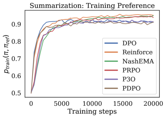
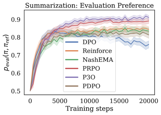
Figure 7: Training vs. evaluation dynamics for summarization. The horizontal axis shows the number of training steps, and the vertical axis shows the preference of the learned policies against $\pi_{\mathrm{ref}}$. We use the same hyperparameters for each method as in Figure 1. (Left) The training preference is measured by $p_{\mathrm{mle}}$ for preference-based methods and by $p_{\mathrm{BTL}}(r_{\mathrm{mle}})$ for RLHF methods. (Right) The evaluation preference measured is by Gemini 1.5 Flash (repeated from Figure 1).

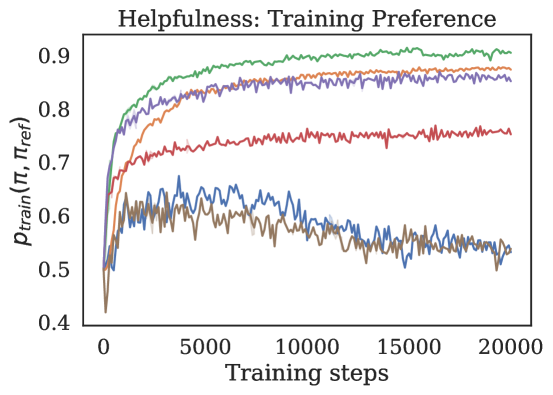
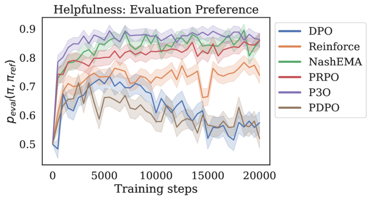
Figure 8: Training vs. evaluation dynamics for helpfulness. The horizontal axis shows the number of training steps, and the vertical axis shows the preference of the learned policies against $\pi_{\mathrm{ref}}$. We use the same hyperparameters for each method as in Figure 1. (Left) The training preference is measured by $p_{\mathrm{mle}}$ for preference-based methods and by $p_{\mathrm{BTL}}(r_{\mathrm{mle}})$ for RLHF methods. (Right) The evaluation preference is measured by Gemini 1.5 Flash.

Figure 7 and Figure 8 presents the learning curves for different methods over a period of either $20,\!000$ training steps or $10,\!000$ training steps (for the larger 8B models). As we note in the curves, the far left side corresponds to the starting point where $\pi_{1}\doteq\pi_{\mathrm{ref}}$, and hence the initial preference is 0.5. In the left figure we can see that all methods consistently seem to be improving on the training reward, where in fact REINFORCE actually seems to be doing better than pessimistic methods. However, that ordering is not followed when evaluated with the much bigger eval model (i.e., Gemini 1.5), as seen in the right figure, wherein pessimistic methods (P3O, PRPO) outperform the standard RLHF methods, and do not degrade over time.

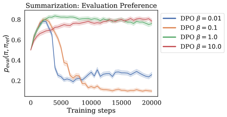
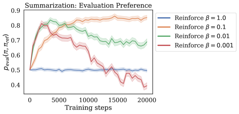
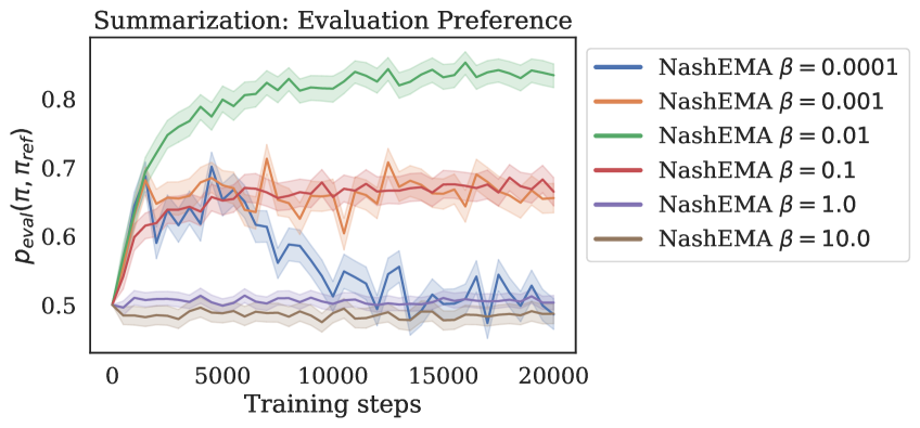
Figure 9: Ablation of RLHF methods for summarization. The horizontal axis indicates the number of training steps, and the vertical axis shows the preference of the learned policies against $\pi_{\mathrm{ref}}$, as measured by Gemini 1.5 Flash. Hyperparameters are selected for the best evaluation performance. (Left) Effect of $\beta$ (KL regularization) on DPO. (Right) Effect of $\beta$ (KL regularization) on REINFORCE. (Bottom) Effect of $\beta$ (KL regularization) on Nash-EMA. Shaded areas represent $95\%$ confidence bands of the evaluation.

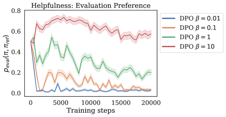
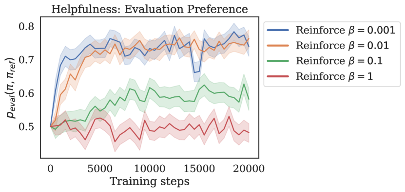
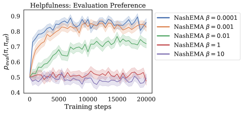
Figure 10: Ablation of RLHF methods for helpfulness. The horizontal axis indicates the number of training steps, and the vertical axis shows the preference of the learned policies against $\pi_{\mathrm{ref}}$, as measured by Gemini 1.5 Flash. (Left) Effect of $\beta$ (KL regularization) on DPO. (Right) Effect of $\beta$ (KL regularization) on REINFORCE. (Bottom) Effect of $\beta$ (KL regularization) on Nash-EMA. Shaded areas represent $95\%$ confidence bands of the evaluation.

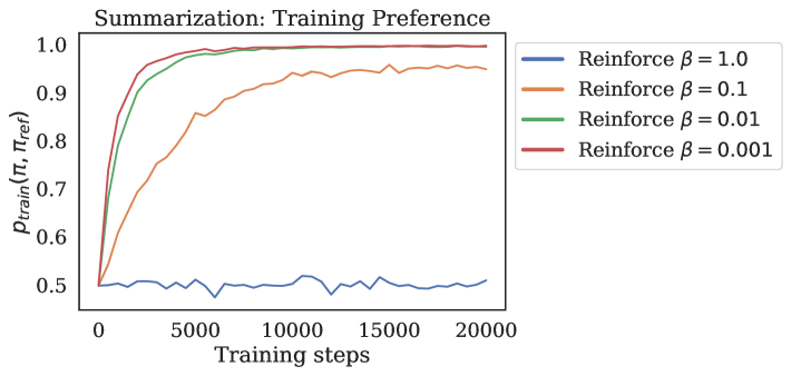
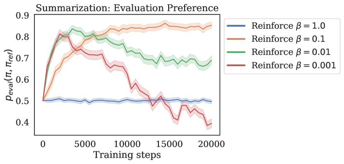
Figure 11: Reward hacking in the case of REINFORCE on summarization. The horizontal axis shows the number of training steps, and the vertical axis shows the preference of the learned policies against $\pi_{\mathrm{ref}}$ using $p_{\mathrm{BTL}}(r_{\mathrm{mle}})$ (left) and Gemini 1.5 Flash (right). REINFORCE exhibits reward hacking particularly for $\beta\in\{0.01,0.001\}$, where the preference on the training reward seems to be stable, i.e., close 1, but the performances constantly degrades on evaluation preferences.

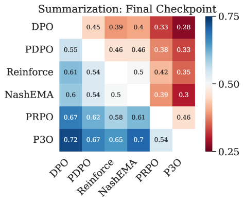
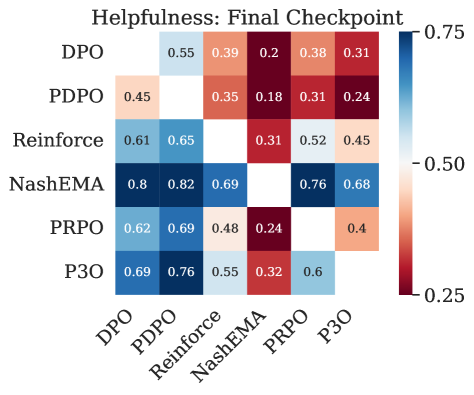
Figure 13: Confusion matrix showing the pairwise evaluation across the different methods for each method’s last checkpoint. On the summarization task especially, the pessimistic models do not appear to degrade with longer training, resulting in even stronger win-rates over the other RLHF baselines (compare to Figure 5).

H.1 Ablations of the RLHF methods

A common approach to mitigating over-optimization in standard RLHF is to adjust the level of KL regularization. Hence, we vary $\beta\in\{10^{i}:i\in\{-5,-4,\ldots,1\}\}$ across a wide range. Evaluations with a larger model reveal that both DPO and REINFORCE degrade significantly for small $\beta$ values ($\beta\in\{10^{-5},10^{-4}\}$). Figure 9 shows these RLHF methods over a more moderate set of $\beta$ values for summarization. We observe that smaller $\beta$ values are more prone to reward hacking for both methods. Notably, DPO reaches its highest peak at $\beta=1.0$, while REINFORCE peaks at $\beta=0.1$. On Helpfulness (Figure 10), DPO also requires particularly large values of $\beta$ to avoid hacking, whereas REINFORCE and Nash-EMA still do well under $p_{\mathrm{eval}}$ with lower $\beta$-values (albeit with very large qualitative regressions—long length, high prevalence of list responses—per Figure 4).

H.2 Detailed setup of the empirical evaluation

Hyper-parameters: Policy is trained for $20,\!000$ steps, where each steps corresponds to a gradient step performed on a given mini-batch. Tables 1-4 presents the hyper-parameters sweeped over for different methods. Parameters in bold (over sweeps) were the final ones used.

Table 1: Hyperparameters for P3O and PRPO for Summarization (TL;DR)

Hyperparameter	Value / Range
Training Steps	$20,\!000$
Mini-Batch Size	$32$
Policy Learning Rate $\eta_{\pi}$	$10^{-5}$
Preference Learning Rate $\eta_{p}$	$\{\mathbf{2.5\times 10^{-5}},\;{5\times 10^{-5}}\}$
Regularization Coefficient $\beta$	$10^{-5}$
$\lambda$ (Sweep)	$\{1,\;2,\;4,\;8,\;16,\;\textbf{32},\;64\}$
EMA Parameter $\gamma$	$0.0025$
Policy Mixing $\alpha$	$\{\textbf{0.0},0.01,0.1,0.25,0.5\}$
Context Length	$1024$
Generation Length	$128$

Table 2: Hyperparameters for RLHF methods (DPO, REINFORCE, Nash-EMA) for Summarization (TL;DR)

Hyperparameter	Value / Range
Training Steps	$20,\!000$
Mini-Batch Size	$32$
Policy Learning Rate $\eta_{\pi}$	$10^{-5}$
Regularization Coefficient $\beta$ (Sweep)	$\{10^{-5},10^{-4},10^{-3},\mathbf{10^{-2}},\textbf{0.1},\textbf{1.0},10.0\}$
Context Length	$1024$
Generation Length	$128$

Table 3: Hyperparameters for P3O and PRPO for Helpfulness

Hyperparameter	Value / Range
Training Steps	$20,\!000$
Mini-Batch Size	$16$
Policy Learning Rate $\eta_{\pi}$	$10^{-5}$
Preference Learning Rate $\eta_{p}$	$5\times 10^{-5}$
Regularization Coefficient $\beta$	$10^{-5}$
$\lambda$ (Sweep)	$\{{32},\;\mathbf{64}\}$
EMA Parameter $\gamma$	$0.0025$
Policy Mixing $\alpha$	$\{\textbf{0.0},0.5\}$
Context Length	1024
Generation Length	128

Table 4: Hyperparameters for RLHF methods (DPO, REINFORCE, Nash-EMA) for Helpfulness

Hyperparameter	Value / Range
Training Steps	$20,\!000$
Mini-Batch Size	$16$
Policy Learning Rate $\eta_{\pi}$	$10^{-5}$
Regularization Coefficient $\beta$ (Sweep)	$\{\mathbf{10^{-4}},\mathbf{10^{-3}},10^{-2},0.1,1.0,\mathbf{10.0}\}$
Context Length	1024
Generation Length	128

Evaluation: We save a checkpoint for policies at every $500$ steps, and generate summaries from $\pi_{t}$ for evaluation. To evaluate the learned model, we query Gemini 1.5 Flash (Gemini Team, 2024) to judge which summary is better for the given input context. The evaluation prompts are shown below.

To avoid any positional bias, we make two queries for each comparison, where we swap the order of the two generations.

Appendix I Sample Generations

I.1 Summarization

The following are a number of sample generations from the best checkpoints with each method on the summarization dataset. In agreement with Figure 4, DPO, REINFORCE and NashEMA tend to give longer and more extractive summaries, while the coherency of DPO’s summaries also suffers. Both PRPO and P3O tend to give shorter, succinct summaries.

I.2 Helpfulness

The following are a number of sample generations from the best checkpoints with each method on the helpfulness dataset. Broadly speaking, one can see from the generations that the selected DPO model (with high $\beta$ regularization) does not deviate too far from the reference model, while the REINFORCE and Nash-EMA models nearly always gives long, wordy responses that try to be overly informative, with the REINFORCE model in particular also exhibiting a high prevalence of repeated key-words, phrasings, or tokens (“You are right”, “sure”, “*”, lists). PRPO and P3O generations tend to be more detailed than the reference (though it is not immune to hallucination), and use lists only when appropriate.

References

• Ahmadian et al. (2024) Ahmadian, A., Cremer, C., Gallé, M., Fadaee, M., Kreutzer, J., Pietquin, O., Üstün, A., and Hooker, S. Back to Basics: Revisiting REINFORCE Style Optimization for Learning from Human Feedback in LLMs, 2024.
• Amodei et al. (2016) Amodei, D., Olah, C., Steinhardt, J., Christiano, P., Schulman, J., and Mané, D. Concrete Problems in AI Safety, 2016.
• Anil et al. (2023) Anil, R., Dai, A. M., Firat, O., Johnson, M., Lepikhin, D., Passos, A., Shakeri, S., Taropa, E., Bailey, P., Chen, Z., et al. Palm 2 technical report. arXiv preprint arXiv:2305.10403, 2023.
• Antos et al. (2007) Antos, A., Szepesvári, C., and Munos, R. Fitted q-iteration in continuous action-space mdps. Advances in neural information processing systems, 20, 2007.
• Antos et al. (2008) Antos, A., Szepesvári, C., and Munos, R. Learning near-optimal policies with bellman-residual minimization based fitted policy iteration and a single sample path. Machine Learning, 71:89–129, 2008.
• Azar et al. (2023) Azar, M. G., Rowland, M., Piot, B., Guo, D., Calandriello, D., Valko, M., and Munos, R. A General Theoretical Paradigm to Understand Learning from Human Preferences, 2023.
• Bai et al. (2022) Bai, Y., Jones, A., Ndousse, K., Askell, A., Chen, A., DasSarma, N., Drain, D., Fort, S., Ganguli, D., Henighan, T., et al. Training a helpful and harmless assistant with reinforcement learning from human feedback. arXiv preprint arXiv:2204.05862, 2022.
• Ben-Tal et al. (2013) Ben-Tal, A., den Hertog, D., De Waegenaere, A., Melenberg, B., and Rennen, G. Robust solutions of optimization problems affected by uncertain probabilities. Manage. Sci., 59(2):341–357, February 2013. ISSN 0025-1909. doi: 10.1287/mnsc.1120.1641. URL https://doi.org/10.1287/mnsc.1120.1641.
• Bertsimas & Sim (2004) Bertsimas, D. and Sim, M. The price of robustness. Operations research, pp.  35–53, 2004.
• Bradley & Terry (1952) Bradley, R. A. and Terry, M. E. Rank analysis of incomplete block designs: I. the method of paired comparisons. Biometrika, 39(3/4):324–345, 1952.
• Buckman et al. (2020) Buckman, J., Gelada, C., and Bellemare, M. G. The importance of pessimism in fixed-dataset policy optimization. arXiv preprint arXiv:2009.06799, 2020.
• Calandriello et al. (2024) Calandriello, D., Guo, D., Munos, R., Rowland, M., Tang, Y., Pires, B. A., Richemond, P. H., Lan, C. L., Valko, M., Liu, T., Joshi, R., Zheng, Z., and Piot, B. Human Alignment of Large Language Models through Online Preference Optimisation, 2024.
• Cen et al. (2024) Cen, S., Mei, J., Goshvadi, K., Dai, H., Yang, T., Yang, S., Schuurmans, D., Chi, Y., and Dai, B. Value-Incentivized Preference Optimization: A Unified Approach to Online and Offline RLHF, 2024.
• Chen & Jiang (2019) Chen, J. and Jiang, N. Information-theoretic considerations in batch reinforcement learning. In International Conference on Machine Learning, pp. 1042–1051. PMLR, 2019.
• Cheng et al. (2022) Cheng, C.-A., Xie, T., Jiang, N., and Agarwal, A. Adversarially trained actor critic for offline reinforcement learning. In International Conference on Machine Learning, pp. 3852–3878. PMLR, 2022.
• Christiano et al. (2017) Christiano, P. F., Leike, J., Brown, T., Martic, M., Legg, S., and Amodei, D. Deep reinforcement learning from human preferences. Advances in neural information processing systems, 30, 2017.
• Coste et al. (2023) Coste, T., Anwar, U., Kirk, R., and Krueger, D. Reward model ensembles help mitigate overoptimization. arXiv preprint arXiv:2310.02743, 2023.
• Cui & Du (2022) Cui, Q. and Du, S. S. When is Offline Two-Player Zero-Sum Markov Game Solvable?, 2022.
• Eisenstein et al. (2024) Eisenstein, J., Nagpal, C., Agarwal, A., Beirami, A., D’Amour, A., Dvijotham, D. J., Fisch, A., Heller, K., Pfohl, S., Ramachandran, D., Shaw, P., and Berant, J. Helping or Herding? Reward Model Ensembles Mitigate but do not Eliminate Reward Hacking, 2024.
• Farahmand et al. (2010) Farahmand, A.-m., Szepesvári, C., and Munos, R. Error propagation for approximate policy and value iteration. Advances in neural information processing systems, 23, 2010.
• Fisch et al. (2024) Fisch, A., Eisenstein, J., Zayats, V., Agarwal, A., Beirami, A., Nagpal, C., Shaw, P., and Berant, J. Robust preference optimization through reward model distillation. arXiv preprint arXiv:2405.19316, 2024.
• Fujimoto et al. (2019) Fujimoto, S., Meger, D., and Precup, D. Off-policy deep reinforcement learning without exploration. In International conference on machine learning, pp. 2052–2062. PMLR, 2019.
• Gao et al. (2023) Gao, L., Schulman, J., and Hilton, J. Scaling laws for reward model overoptimization. In International Conference on Machine Learning, pp. 10835–10866. PMLR, 2023.
• Gemini Team (2024) Gemini Team. Gemini: A family of highly capable multimodal models, 2024. URL https://arxiv.org/abs/2312.11805.
• Guo et al. (2024) Guo, S., Zhang, B., Liu, T., Liu, T., Khalman, M., Llinares, F., Rame, A., Mesnard, T., Zhao, Y., Piot, B., Ferret, J., and Blondel, M. Direct Language Model Alignment from Online AI Feedback, 2024.
• Huang et al. (2024a) Huang, A., Zhan, W., Xie, T., Lee, J. D., Sun, W., Krishnamurthy, A., and Foster, D. J. Correcting the mythos of kl-regularization: Direct alignment without overparameterization via chi-squared preference optimization. arXiv preprint arXiv:2407.13399, 2024a.
• Huang et al. (2024b) Huang, A., Zhan, W., Xie, T., Lee, J. D., Sun, W., Krishnamurthy, A., and Foster, D. J. Correcting the Mythos of KL-Regularization: Direct Alignment without Overoptimization via Chi-Squared Preference Optimization. https://arxiv.org/abs/2407.13399v2, 2024b.
• Jaques et al. (2019) Jaques, N., Ghandeharioun, A., Shen, J. H., Ferguson, C., Lapedriza, A., Jones, N., Gu, S., and Picard, R. Way off-policy batch deep reinforcement learning of implicit human preferences in dialog. arXiv preprint arXiv:1907.00456, 2019.
• Jin et al. (2021) Jin, Y., Yang, Z., and Wang, Z. Is pessimism provably efficient for offline rl? In International Conference on Machine Learning, pp. 5084–5096. PMLR, 2021.
• Jordan et al. (1999) Jordan, M. I., Ghahramani, Z., Jaakkola, T. S., and Saul, L. K. An introduction to variational methods for graphical models. Machine learning, 37:183–233, 1999.
• Kidambi et al. (2020) Kidambi, R., Rajeswaran, A., Netrapalli, P., and Joachims, T. Morel: Model-based offline reinforcement learning. Advances in neural information processing systems, 33:21810–21823, 2020.
• Koppel et al. (2024) Koppel, A., Bhatt, S., Guo, J., Eappen, J., Wang, M., and Ganesh, S. Information-directed pessimism for offline reinforcement learning. In Forty-first International Conference on Machine Learning, 2024.
• Kostrikov et al. (2021) Kostrikov, I., Nair, A., and Levine, S. Offline reinforcement learning with implicit q-learning. arXiv preprint arXiv:2110.06169, 2021.
• Kumar et al. (2019) Kumar, A., Fu, J., Soh, M., Tucker, G., and Levine, S. Stabilizing off-policy q-learning via bootstrapping error reduction. Advances in neural information processing systems, 32, 2019.
• Kumar et al. (2020) Kumar, A., Zhou, A., Tucker, G., and Levine, S. Conservative q-learning for offline reinforcement learning. Advances in Neural Information Processing Systems, 33:1179–1191, 2020.
• Laroche et al. (2019) Laroche, R., Trichelair, P., and Des Combes, R. T. Safe policy improvement with baseline bootstrapping. In International conference on machine learning, pp. 3652–3661. PMLR, 2019.
• Liu et al. (2020) Liu, Y., Swaminathan, A., Agarwal, A., and Brunskill, E. Provably good batch off-policy reinforcement learning without great exploration. Advances in neural information processing systems, 33:1264–1274, 2020.
• Liu et al. (2024) Liu, Z., Lu, M., Zhang, S., Liu, B., Guo, H., Yang, Y., Blanchet, J., and Wang, Z. Provably Mitigating Overoptimization in RLHF: Your SFT Loss is Implicitly an Adversarial Regularizer, 2024.
• Luce (2012) Luce, R. Individual Choice Behavior: A Theoretical Analysis. Dover Books on Mathematics. Dover Publications, 2012. ISBN 9780486153391. URL https://books.google.com/books?id=ERQsKkPiKkkC.
• Munos (2003) Munos, R. Error bounds for approximate policy iteration. In ICML, volume 3, pp.  560–567. Citeseer, 2003.
• Munos & Szepesvári (2008) Munos, R. and Szepesvári, C. Finite-time bounds for fitted value iteration. Journal of Machine Learning Research, 9(5), 2008.
• Munos et al. (2023) Munos, R., Valko, M., Calandriello, D., Azar, M. G., Rowland, M., Guo, Z. D., Tang, Y., Geist, M., Mesnard, T., Michi, A., Selvi, M., Girgin, S., Momchev, N., Bachem, O., Mankowitz, D. J., Precup, D., and Piot, B. Nash Learning from Human Feedback, 2023.
• Ouyang et al. (2022) Ouyang, L., Wu, J., Jiang, X., Almeida, D., Wainwright, C., Mishkin, P., Zhang, C., Agarwal, S., Slama, K., Ray, A., et al. Training language models to follow instructions with human feedback. Advances in neural information processing systems, 35:27730–27744, 2022.
• Park et al. (2024) Park, R., Rafailov, R., Ermon, S., and Finn, C. Disentangling Length from Quality in Direct Preference Optimization, 2024.
• Rafailov et al. (2023) Rafailov, R., Sharma, A., Mitchell, E., Ermon, S., Manning, C. D., and Finn, C. Direct Preference Optimization: Your Language Model is Secretly a Reward Model, 2023.
• Raffel et al. (2020) Raffel, C., Shazeer, N., Roberts, A., Lee, K., Narang, S., Matena, M., Zhou, Y., Li, W., and Liu, P. J. Exploring the limits of transfer learning with a unified text-to-text transformer. Journal of machine learning research, 21(140):1–67, 2020.
• Roberts et al. (2023) Roberts, A., Chung, H. W., Mishra, G., Levskaya, A., Bradbury, J., Andor, D., Narang, S., Lester, B., Gaffney, C., Mohiuddin, A., et al. Scaling up models and data with t5x and seqio. Journal of Machine Learning Research, 24(377):1–8, 2023.
• Singhal et al. (2023) Singhal, P., Goyal, T., Xu, J., and Durrett, G. A long way to go: Investigating length correlations in rlhf. arXiv preprint arXiv:2310.03716, 2023.
• Stiennon et al. (2020) Stiennon, N., Ouyang, L., Wu, J., Ziegler, D., Lowe, R., Voss, C., Radford, A., Amodei, D., and Christiano, P. F. Learning to summarize with human feedback. Advances in Neural Information Processing Systems, 33:3008–3021, 2020.
• Swamy et al. (2024) Swamy, G., Dann, C., Kidambi, R., Wu, Z. S., and Agarwal, A. A Minimaximalist Approach to Reinforcement Learning from Human Feedback, 2024.
• Tang et al. (2024) Tang, Y., Guo, Z. D., Zheng, Z., Calandriello, D., Munos, R., Rowland, M., Richemond, P. H., Valko, M., Pires, B. Á., and Piot, B. Generalized Preference Optimization: A Unified Approach to Offline Alignment, 2024.
• Völske et al. (2017) Völske, M., Potthast, M., Syed, S., and Stein, B. Tl; dr: Mining reddit to learn automatic summarization. In Proceedings of the Workshop on New Frontiers in Summarization, pp.  59–63, 2017.
• Wang et al. (2020) Wang, R., Foster, D. P., and Kakade, S. M. What are the statistical limits of offline rl with linear function approximation? ArXiv, abs/2010.11895, 2020. URL https://api.semanticscholar.org/CorpusID:225039786.
• Willams (1992) Willams, R. J. Simple statistical gradient-following algorithms for connectionist reinforcement learning. Machine learning, 8:229–256, 1992.
• Wu et al. (2019) Wu, Y., Tucker, G., and Nachum, O. Behavior regularized offline reinforcement learning. arXiv preprint arXiv:1911.11361, 2019.
• Xiao et al. (2023) Xiao, C., Wang, H., Pan, Y., White, A., and White, M. The in-sample softmax for offline reinforcement learning. arXiv preprint arXiv:2302.14372, 2023.
• Xie & Jiang (2020) Xie, T. and Jiang, N. Q* approximation schemes for batch reinforcement learning: A theoretical comparison. In Conference on Uncertainty in Artificial Intelligence, pp. 550–559. PMLR, 2020.
• Xie et al. (2021) Xie, T., Cheng, C.-A., Jiang, N., Mineiro, P., and Agarwal, A. Bellman-consistent pessimism for offline reinforcement learning. Advances in neural information processing systems, 34:6683–6694, 2021.
• Ye et al. (2024) Ye, C., Xiong, W., Zhang, Y., Jiang, N., and Zhang, T. Online Iterative Reinforcement Learning from Human Feedback with General Preference Model, 2024.
• Yu et al. (2020) Yu, T., Thomas, G., Yu, L., Ermon, S., Zou, J. Y., Levine, S., Finn, C., and Ma, T. Mopo: Model-based offline policy optimization. Advances in Neural Information Processing Systems, 33:14129–14142, 2020.
• Zanette et al. (2021) Zanette, A., Wainwright, M. J., and Brunskill, E. Provable benefits of actor-critic methods for offline reinforcement learning. Advances in neural information processing systems, 34:13626–13640, 2021.
• Zhang et al. (2024) Zhang, D., Lyu, B., Qiu, S., Kolar, M., and Zhang, T. Pessimism meets risk: risk-sensitive offline reinforcement learning. arXiv preprint arXiv:2407.07631, 2024.
• Zhang et al. (2023) Zhang, Y., Bai, Y., and Jiang, N. Offline learning in markov games with general function approximation. In International Conference on Machine Learning, pp. 40804–40829. PMLR, 2023.