Stochastic Optimal Control of an Epidemic Under Partial Information

Abstract

In this paper, we address a social planner’s optimal control problem for a partially observable stochastic epidemic model. The control measures include social distancing, testing, and vaccination. Using a diffusion approximation for the state dynamics of the epidemic, we apply filtering arguments to transform the partially observable stochastic optimal control problem into an optimal control problem with complete information. This transformed problem is treated as a Markov decision process. The associated Bellman equation is solved numerically using optimal quantization methods for approximating the expectations involved to mitigate the curse of dimensionality. We implement two approaches, the first involves state discretization coupled with linear interpolation of the value function at non-grid points. The second utilizes a parametrization of the value function with educated ansatz functions. Extensive numerical experiments are presented to demonstrate the efficacy of both methods.

1 Introduction

In order to respond to an epidemic efficiently, policy makers have to assess the potential efficacy of various strategies for containing, mitigating, or even eradicating the disease. Such an assessment involves first the modeling of plausible scenarios for the future course of the epidemic, second the identification of preventive measures and pharmaceutical measures when available, that can be implemented to limit the epidemic spread, and third the evaluation of the costs and impacts of intervention. The optimal control of an epidemic has been subject to a massive interest in the recent years, largely due to the Covid-19 pandemic. This procedure is of particular relevance because of the conflicting interests of the governments between a safety-oriented approach (limiting the death due to the disease) and an economy-focused approach (avoid high economy burden). The formulation of an optimal control problem for an epidemic requires the description of the epidemic dynamics. Mathematical modeling plays an important role in this process by allowing to construct specific models that capture essential features of the disease of interest. The compartmental model, first proposed by Kermack and McKendrick (1927), is the most widely used approach in epidemiology. These models divide the entire population into distinct compartments according to the state of health with respect to the disease under study. In that paper, the resulting dynamics of the compartmental model is described by a system of ordinary differential equations (ODEs). ODE models are a popular choice among authors and deterministic optimal control for epidemic are built on top of such ODE models. Furthermore, extensions to stochastic dynamics are possible and more realistic, since they allow for the incorporation of randomness that cannot be predicted during an epidemic.

Literature review on optimal control of epidemics

When facing an epidemic outbreak, measures that aim at least at containing the spread of the disease have to be enforced, since eradication or suppression is both costly and unrealistic. Quite often, cure and vaccine are not available, and authorities need to rely on non-pharmaceutical intervention (NPI) such as social distancing, home quarantine, lockdown of non-essential businesses and other institutions. Additionally, preventive measures such as use of face masks may also be employed. This was pointed out for the recent Covid-19 pandemic by Kantner and Koprucki (2020), Hellewell et al. (2020), Ferguson et al. (2020) who conducted analyses to assess the efficacy of NPI. The most widely considered NPI is social distancing, which allows for a reduction in social interactions and, consequently, the prevention of contact between susceptible and infectious individuals. The optimal level of social distancing and the timing have been investigated by several authors including Miclo et al. (2022), Kruse and Strack (2020), Behncke (2000), Nowzari et al. (2016), Federico and Ferrari (2021), Alvarez et al. (2020), Calvia et al. (2024) and Charpentier et al. (2020). More specifically, Kruse and Strack (2020) introduced a parameter that is controlled by the planer allowing to adjust the lockdown level. Given that they considered linear cost in the number of infected, the resulting optimal control strategy is of the bang-bang type. Miclo et al. (2022) provided an analytic policy for their optimal control problem with ICU constraints. Alvarez et al. (2020) numerically characterized the optimal lockdown policy for a SIR model. Charpentier et al. (2020) considered a control problem with asymptomatic compartments and provided numerical solution to the optimal policy. Moreover, Acemoglu et al. (2021) proposed a targeted lockdown on a more vulnerable age-grouped model, demonstrating that targeted lockdowns policies outperform indiscriminated policies.

The main objective of these NPI is to flatten the infection curve in order to avoid overwhelming of the healthcare system’s capacity. In this regards, Charpentier et al. (2020), Miclo et al. (2022), Avram et al. (2022) consider optimal control problems with ICU constraints. Miclo et al. (2022) observed that flattening the curve strategy is suboptimal and suggest the so called ”filling the box” strategy which consists of four phases. First, the spread of the disease is let freely and then as the ICU limit is approached, a strong lockdown is applied. After the lockdown, regulations are gradually lifted maintaining the rate of infection constants and in the last phase all regulations are lifted. Kantner and Koprucki (2020), and Ferguson et al. (2020) recommended exploring NPI strategies that goes beyond flattening the curve.

Beside NPI, vaccination has been considered as a highly effective strategy for eradicating, or at the very least containing, an epidemic. The smallpox vaccine has been successful in eradication and the vaccination has reduced death due to measles by $94\%$. This explain why many studies on epidemic control have focused on vaccination, see Hethcote and Waltman (1973), see also, Ledzewicz and Schättler (2011), Hu and Zou (2013), Laguzet and Turinici (2015). In some authors’ models, vaccinated people are grouped in an additional compartment (Ishikawa (2012), Garriga et al. (2022)). Furthermore, Federico et al. (2024) examined an optimal vaccination problem with incomplete immunization power of the vaccine, analyzing the problem with the dynamic programming approach. Hansen and Day (2011) investigate the use of isolation and vaccination in a model incorporating limited resources. In some models, the arrival time of the vaccine is random, as observed in Garriga et al. (2022) and Federico et al. (2024).

When it comes to solution approaches to epidemic control problems, the Pontryagin maximum principle is widely employed. This requires convexity conditions on the objective function. Non-convex (in the state dynamics or in the objective function) optimization problems are notoriously difficult to study with the maximum principle approach. These convexity conditions restrict the class of functions that can be included in the cost functional. However, Calvia et al. (2024) noted that the dynamic programming approach can be profitably applied to the optimal control problems for epidemics with less restrictive conditions on the objective functional. Therefore, they analyzed a non-convex epidemic control problem using the dynamic programming approach. They proved a continuity property of the value function and showed that the value function is a solution of the HJB equation in the viscosity sense. Similarly, Federico and Ferrari (2021); Federico et al. (2024) used the dynamic programming technique and the viscosity solution concept.

Problem statement

In this study, we consider a population which is divided into classes according to the state of health concerning a given disease. The classes are susceptible $S$, non-detected infected $I^{-}$, detected infected $I^{+}$, non-detected recovered $R^{-}$, detected recovered $R^{+}$, and hospitalized $H$. This model is denoted by $SI^{\pm}R^{\pm}H$ and transitions between compartments are depicted in Figure 1. This flowchart is similar to that of Charpentier et al. (2020) which accounts for asymptomatic compartments with unobservable compartment sizes. Such unobserved sizes could also result from unreported cases of infection during an epidemic. Al-Tawfiq (2020) and Day (2020) highlight the potentially high rate of asymptomatic individuals for the Covid-19. A more detailed description of the the model in Figure 1 is provided in Section 3. The dynamics of our model are described by a stochastic process using the approximation of a continuous time Markov chain (CTMC) by a diffusion process as presented in Britton et al. (2019) and in our papers Ouabo Kamkumo et al. (2025); Mbouandi Njiasse et al. (2025). Moreover, we assume a situation where the vaccine is already available and thus the social planner could select three control measures, namely social distancing, testing to detect more infectious individuals and vaccination.

Figure 1: Flowchart of the $SI^{\pm}R^{\pm}H$ compartmental model with control variables $u^{L},u^{T}$ and $u^{V}$. Hidden compartments are in red and observable compartments in blue.

We then formulate the social planner’s control problem by constructing realistic costs that account for both the economic and sanitary impacts of intervention measures. These costs include fixed costs that the government must bear as long as a specific control measure is in place. Additionally, the primary component of each cost is linear, and depends on the number of people affected by the particular control measure. The final component is a quadratic penalty applied when a certain threshold is exceeded, making it less likely for strategies that lead to exceeding this threshold to be selected. The resulting problem is a stochastic optimal control problem (SOCP) with partially observed state process $X_{n}=(I^{-}_{n},R^{-}_{n},I^{+}_{n},R^{+}_{n},H_{n})^{\top},n=0,\ldots,N_{t}$, where $N_{t}$ is the time index of the time horizon, that is also called SOCP under partial information. We employ the innovations approach of stochastic filtering to transform the initial SOCP with partially observed state process into a corresponding SOCP with fully observed state process by replacing the hidden state components $Y_{n}=(I^{-}_{n},R^{-}_{n})^{\top}$ by its extended Kalman filter. The latter is characterized by the approximations of the conditional mean $M_{n}$ and conditional covariance $Q_{n}$. A more detailed examination of these concepts can be found in Section 2.4. We then consider the problem as a Markov decision process (MDP) and derive the associated Bellman equation.

Our contribution

The originality of this model lies in the fact that it allows to describe diseases with asymptomatic individuals, even though the number of asymptomatic individuals is not observable, and to address the problem of "flattening the curve" with a modeling of hospital facilities. Decision makers need to ensure that the maximum capacity of hospital equipment is not reached to avoid the ethical triage problem. In addition to formulating the SOCP of an epidemic with a special feature, namely, the partial information aspect, we provide numerical solutions to the SOCP, which suffers from the curse of dimensionality due to an 8-dimensional state process and a 3-dimensional control. To address this challenge, the Bellman equation is solved numerically through state space discretization. The conditional expectation in the Bellman equation is then approximated by quantization techniques, which involve replacing a continuous random variable with an appropriate discrete random variable. Two implementations of the backward recursion algorithm are performed. The first uses state space discretization, quantization and linear interpolation of the value function, while the second combines state space discretization, quantization and least squares parametrization of the value function with well-chosen ansatz basis functions. Both implementations yield similar results, providing the optimal decision rule and the associated optimal cost or value function. Simulations of the epidemic path, using the derived optimal control strategies, demonstrate their effectiveness in containing the spread of the epidemic.

Paper organization

Section 2 details the compartmental model, control measures, and the stochastic dynamics of the compartment sizes. Section 3 focuses on the formulation of the SOCP under partial information using the filtering argument. In Section 4, we present numerical methods based on the backward recursion algorithm and optimal quantization. Section 5 features extensive numerical experiments performed using both approaches. Finally, appendices compile some intermediate numerical experiments that were omitted from the main text.

2 Model description

2.1 Compartmental model

Compartmental models are the most powerful tools for monitoring and predicting the evolution of an epidemic. Each epidemic must be described by a specific compartmental model that captures all the important features of the epidemic. Therefore, we consider the $SI^{\pm}R^{\pm}H$ compartmental epidemic model in Figure 1, which is an extension of the classical and well-known $SIR$ model. In this modified model, the total population $N$, that we assume to be constant throughout the study period, is divided into compartments according to the epidemic status of individuals within the population. Therefore, the susceptible compartment, denoted by $S$, contains all those who could contract the disease and become infectious. To capture the peculiarities of diseases with asymptomatic individuals, the infectious compartment is split into undetected infectious $I^{-}$ and detected infectious $I^{+}$. Similarly, the recovered compartment is split into undetected recovered $R^{-}$ and detected recovered $R^{+}$. We also include the hospital group $H$, which includes hospitalized individuals and those in special hospital units, such as intensive care units (ICU). This model was inspired by the paper of Charpentier et al. (2020) and we refer the reader to Ouabo Kamkumo et al. (2025) for a more detailed description of such a model.

Several transitions with corresponding intensities are considered. The transition rates are the reciprocal of the average sojourn time in a given compartment and allow to get the average number of transitions per unit of time. We assume that detected infectious persons $I^{+}$ are well isolated and cannot infect susceptible persons, so that new infections are only due to contacts between a susceptible and a non-detected infectious person. The latter transition occurs with intensity $\beta>0$. This means that on average $\beta S{I^{-}}/{N}$ number of people become infectious per unit of time when there are no control measures. Moreover, a non-detected infectious person can be detected with detection rate $\alpha>0$. If the condition of an infected person becomes severe, he/she will be hospitalized with rate $\eta^{-}>0$ if he is not detected, or at a rate $\eta^{+}>0$ if he is detected. Alternatively, infected individuals recover with intensities $\gamma^{-}>0$ if they are not detected, $\gamma^{+}>0$ if they are detected, and $\gamma^{H}>0$ if they recover in a hospital. Finally, in this model we assume that the vaccine is available. Through vaccination, susceptible, non-detected infectious or non-detected recovered individuals can be immunized against the disease and move to the class of detected recovered individuals. In addition, this epidemic flowchart has some non-observable or hidden states $S$, $I^{-}$, and $R^{-}$, namely, because we cannot distinguish between asymptomatic or unreported individuals and susceptible individuals. Hence, we cannot collect data on the number of people in these compartments at any given time. The remaining compartments will be observable since inflows and the outflows of these compartments can mostly be recorded. In this model, we have made the assumption that those who recover from the disease or are vaccinated against it acquire lifelong immunity. At least we assume that the immunity lasts until the time horizon of the study. For this reason, the compartment $R^{+}$ is an absorbing state. Consequently, this model can describe a disease with lifelong immunity or the early stage of a disease that provides immunity after recovery that lasts longer than the time horizon of the study.

2.2 Control measures

The management of an epidemic can be summarized as a problem of cost-optimal containment of the epidemic through an appropriate mix of measures. Decision-makers need to know on which levers they can act to mitigate the spread of the disease within the population. For this epidemic model, we are investigating some potential measures that will be divided into three types: social distancing measures or lock-down, detection or testing measures, and vaccination strategy.

2.2.1 Social distancing or lock-down

Historically, quarantine has been employed to isolate infected individuals and prevent them from contaminating those who have not yet been infected. However, this type of measure is more effective in the early phase of an epidemic and becomes more difficult to implement on a larger scale. Furthermore, the economic cost of such a policy may be too high. Instead, for a large-scale epidemic, we can consider social distancing measures with different levels of restrictions. The level of social distancing will be quantified with the control variable $u^{L}$ which ranges from $0$ to $1$, with $0$ corresponding to the absence of social distancing, while the value $1$ represents a strict and perfect lock-down (which is not achievable in reality). These control variables involve other NPI measures such as wearing masks in public places and mobility restrictions. The implementation of the control variable $u^{L}$ will result in a reduction of the transmission rate from $\beta$ to $(1-u^{L})\beta$.

2.2.2 Detection or testing

Accurate determination of the actual number of infectious individuals is of critical relevance in the assessment of the current state of the epidemic and its future evolution. A good testing strategy allows for the identification, tracking, and isolation of infected individuals if necessary. The testing control variable may range from a minimum testing rate $u^{T}_{min}\geq 0$ when almost no specific testing policy is applied, to the maximum possible testing strategy $u^{T}_{max}$ that policymakers can afford. The lower limit $u^{T}_{min}$ may eventually be zero if no detection measures are applied. In the model, it is assumed that the expected number of detections per unit of time is proportional to the testing rate $u^{T}$. In other words, the greater the number of tests performed, the greater the proportion of non-detected infected individuals who are detected.

2.2.3 Vaccination

The most effective method for eradicating an epidemic is through a large-scale vaccination campaign. In the fight for total eradication of the disease, the government has as one of its main objectives, to make a vaccine available to the population for prevention. When designing a vaccination strategy, several questions arise such as the quantity of vaccine to be produced and also the vaccination coverage to be established. Unfortunately, planning and executing these strategies have financial costs. The decision maker must consider the problem of controlling the rate of individuals to be vaccinated at a given time. Before proceeding, we introduce $u^{V}\geq 0$, a control variable that controls the average intensity of individuals who receive the vaccine per unit of time. In addition, the upper limit of the vaccination intensity that the policymakers can afford to have in place is denoted by $u^{V}_{max}$.

2.3 Stochastic dynamics of the compartmental model

To describe the dynamic of the above compartmental model in Figure 1, we adopt the continuous-time Markov chain $(CTMC)$ approach as described in Anderson and Kurtz (2011); Britton et al. (2019); Guy et al. (2015) and Ouabo Kamkumo et al. (2025) . This approach was initially developed to model chemical reaction networks. The dynamics of compartment sizes are described by counting processes which are first replaced by a Poisson process with state dependent intensities. Then, considering the relative subpopulation sizes for $N$ large, the Markov jump process is approximated by a diffusion process, for which the error between both infinitesimal generators is of order $o({1}/{N})$, see Guy et al. (2015). By applying this method, we derive the following diffusion approximation for the $SI^{\pm}R^{\pm}H$ model. It should be noted that for the sake of simplified notation, we omitted the time argument of each component of the state variable in the drift and diffusion coefficients. These coefficients may depend explicitly on the time variable through the infections rate that can be considered time dependent $\beta=\beta(t)$. If we denote the state variable $X=(Y^{\top},Z^{\top})^{\top}$, with $Y=(I^{-},R^{-},S)^{\top}$ and $Z=(I^{+},R^{+},H)^{\top}$, which components represent absolute subpopulation size in each compartment, then it satisfies the following stochastic differential equation (SDE), where the component $S(t)=Y_{3}(t)$ is omitted and can be recovered by normalization $Y_{3}=N-(Y_{1}+Y_{2}+Z_{1}+Z_{2}+Z_{3})$ because we assume that the population size remains constant.

$$d\left(\begin{array}[]{c}Y_{1}\\ Y_{2}\\[1.37775pt] Z_{1}\\ Z_{2}\\ Z_{3}\\ \end{array}\right)\hskip-5.69046pt = \hskip-5.69046pt\left(\begin{array}[]{c}\frac{(1-u^{L})\beta Y_{1}}{N}(N-(Y_{1}+Y_{2}+Z_{1}+Z_{2}+Z_{3}))-(\gamma^{-}+\eta^{-}+u^{T}+u^{V})Y_{1}\\ \gamma^{-}Y_{1}-u^{V}Y_{2}\\[1.37775pt] u^{T}Y_{1}-(\gamma^{+}+\eta^{+})Z_{1}\\ \gamma^{+}Z_{1}+\gamma^{H}Z_{3}+u^{V}(N-(Z_{1}+Z_{2}+Z_{3}))\\ \eta^{-}Y_{1}+\eta^{+}Z_{1}-\gamma^{H}Z_{3}\end{array}\right)dt+\left(\begin{array}[]{cc}\overline{\sigma}&\overline{g}\\ 0&\overline{\ell}\end{array}\right)dW$$

such that when the state is split into hidden state $Y$ and observation $Z$, the diffusion approximation can be expressed as follows:

$$dY(t) =\overline{f}(t,Y(t),Z(t),u(t))dt+\overline{\sigma}(t,Y(t),Z(t),u(t))dW^{1}(t)+\overline{g}(t,Y(t),Z(t),u(t))dW^{2}(t),$$ (2)

$$dZ(t) =(\overline{h}_{0}(t,Z(t),u(t))+\overline{h_{1}}(t,Z(t),u(t))Y(t))dt+\overline{\ell}(t,Y(t),Z(t),u(t))dW^{2}(t).$$ (3)

The drift matrices are defined as:
 
$\overline{f}(t,Y,Z,u)=\left(\begin{array}[]{c}\frac{(1-u^{L})\beta Y_{1}}{N}(N-(Y_{1}+Y_{2}+Z_{1}+Z_{2}+Z_{3}))-(\gamma^{-}+\eta^{-}+u^{T}+u^{V})Y_{1}\\ \gamma^{-}Y_{1}-u^{V}Y_{2}\\ \end{array}\right),$ $\overline{h}_{0}(t,Z,u)~~=\left(\begin{array}[]{c}-(\gamma^{+}+\eta^{+})Z_{1}\\ \gamma^{+}Z_{1}+\gamma^{H}Z_{3}+u^{V}(N-(Z_{1}+Z_{2}+Z_{3}))\\ \eta^{+}Z_{1}-\gamma^{H}Z_{3}\end{array}\right),$ $\overline{h_{1}}(t,Z,u)~~=\left(\begin{array}[]{cc}u^{T}&0\\ 0&0\\ \eta^{-}&0\end{array}\right).$

The matrices in the diffusion coefficient are defined as

$\overline{\sigma}(t,Y,Z,u)$	=	$\left(\begin{array}[]{cc}\sqrt{\frac{(1-u^{L})\beta Y_{1}}{N}(N-(Y_{1}+Y_{2}+Z_{1}+Z_{2}+Z_{3}))}&-\sqrt{\gamma^{-}Y_{1}}\\ 0&\sqrt{\gamma^{-}Y_{1}}\\ \end{array}\right),$
$\overline{g}(t,Y,Z,u)$	$=$	$\left(\begin{array}[]{*{8}{c}}-\sqrt{u^{T}Y_{1}}&0&0&-\sqrt{u^{V}Y_{1}}&0&-\sqrt{\eta^{-}Y_{1}}&0&0\\ 0&0&0&0&-\sqrt{u^{V}Y_{2}}&0&0&0\end{array}\right),$

$\overline{\ell}(t,Y,Z,u)$    $=$

$\left(\begin{array}[]{c@{\hspace*{0.2em}}c@{\hspace*{0.1em}}c@{\hspace*{0.2em}}c@{\hspace*{0.2em}}c@{\hspace*{0.1em}}c@{\hspace*{0.1em}}c@{\hspace*{0.2em}}c@{\hspace*{0.2em}}}\sqrt{u^{T}Y_{1}}\hfil\hskip 1.59998pt&-\sqrt{\gamma^{+}Z_{1}}\hfil\hskip 0.80005pt&0\hfil\hskip 1.59998pt&0\hfil\hskip 1.59998pt&0\hfil\hskip 0.80005pt&0\hfil\hskip 0.80005pt&-\sqrt{\eta^{+}Z_{1}}\hfil\hskip 1.59998pt&0\hfil\hskip 1.59998pt\\ 0\hfil\hskip 1.59998pt&\sqrt{\gamma^{+}Z_{1}}\hfil\hskip 0.80005pt&\sqrt{u^{V}(N-(Y_{1}+Y_{2}+Z_{1}+Z_{2}+Z_{3}))}\hfil\hskip 1.59998pt&\sqrt{u^{V}Y_{1}}\hfil\hskip 1.59998pt&\sqrt{u^{V}Y_{2}}\hfil\hskip 0.80005pt&0\hfil\hskip 0.80005pt&0\hfil\hskip 1.59998pt&\sqrt{\gamma^{H}Z_{3}}\hfil\hskip 1.59998pt\\ 0\hfil\hskip 1.59998pt&0\hfil\hskip 0.80005pt&0\hfil\hskip 1.59998pt&0\hfil\hskip 1.59998pt&0\hfil\hskip 0.80005pt&\sqrt{\eta^{-}Y_{1}}\hfil\hskip 0.80005pt&\sqrt{\eta^{+}Z_{1}}\hfil\hskip 1.59998pt&-\sqrt{\gamma^{H}Z_{3}}\hfil\hskip 1.59998pt\end{array}\right),$

and

$dW=\left(dW_{1},\ldots,dW_{10}\right)^{\top},$ for each transition, an independent Brownian motion is associated.

In the above SDE, we have split the state vector into non-observable components $Y$ and observable components $Z$. We should also note that the independent components of the $10$-dimensional Brownian motion which depicts the noise of transitions between compartments are split into Brownian motion that appear in the observation $Z$, $dW^{1}=\left(\begin{array}[]{*{2}{c@{\hspace*{0.35em}}}}dW_{1},\hfil\hskip 3.50006pt&dW_{2}\hfil\hskip 3.50006pt\end{array}\right)^{\top}$ and those which are only involved in the hidden state $dW^{2}=\left(dW_{3},\ldots,dW_{10}\right)^{\top}$.

Functions $\overline{f},~\overline{\sigma},~\overline{g}$ and $\overline{\ell}$ are clearly nonlinear in the hidden state $Y$. This nonlinearity prevents the use of the standard Kalman filter approach when it comes to filtering problem. Since we aim to solve the optimal control problem which is numerically untractable in continuous-time for high-dimensional state, we perform a time-discretization to mitigate the curse of dimensionality. Moreover, real-world data for an epidemic are also collected in discrete time. Therefore, the Euler-Maruyama scheme, with time discretization $t_{n}=n\Delta t$, $n=0,\ldots,N_{t}$, is employed to derive the discrete dynamics

$$Y_{n+1} =Y_{n}+f(n,Y_{n},Z_{n},u_{n})+\sigma(n,Y_{n},Z_{n},u_{n})\pazocal{B}^{1}_{n+1}+g(n,Y_{n},Z_{n},u_{n})\pazocal{B}^{2}_{n+1},$$ (4)

$$Z_{n+1} =Z_{n}+h_{0}(n,Z_{n},u_{n})+h_{1}(n,Z_{n},u_{n})Y_{n}+\ell(n,Y_{n},Z_{n},u_{n})\pazocal{B}^{2}_{n+1},$$ (5)

where $(\pazocal{B}^{1}_{n})$ and $(\pazocal{B}^{1}_{n})$ are independent sequences of i.i.d. $\pazocal{N}(0,\mathbb{I})$ random vectors. Note that $\mathbb{I}$ is the identity matrix with the corresponding dimension. In this discrete dynamics, terms with $\Delta t$ are incorporated into functions $f,~\sigma,~g,~\ell,~h_{0},\text{and}~h_{1}$ as we have for instance, $f(n,\cdots)=\overline{f}(t_{n},\cdots)\Delta t$, $\sigma(n,\cdots)=\overline{\sigma}(t_{n},\cdots)\sqrt{\Delta t}$ and similarly for the other coefficients. The time discretization is subject to discretization errors that can destroy the normalization. The loss of this property can lead to negative values for the components of $Y$ and $Z$, or to values greater than $N$. To deal with this issue, it is often necessary for the numerical implementation to set minimum and maximum values for the compartment sizes.

2.4 Partial information and filtering

A particular feature of our problem is that the state process $X$ is not fully observable. We will cope with this issue using the projection to the observable filtration. Let us consider our state process $X=(Y^{\top}_{n},Z^{\top}_{n})^{\top},~n=0,\ldots,N_{t}$, described by the discrete dynamic (4) mentioned above. The filtering problem consists in sequentially estimating the hidden state $Y_{n}$ given the observation process $(Z_{j}),~j=0,\ldots,n$ up to time $n$. This filtering problem is non-standard, first, because the signal drift functions $f$ is non-linear in the hidden state $Y$ and second, because the diffusion coefficients $\sigma,~g,~\ell$ depend on the hidden signal $Y$. To solve this non-linear filtering problem, we use the extended Kalman filter approach. This allows us to derive an approximation to the optimal filter which is characterized by the conditional mean $M_{n}:=\mathbb{E}\left(Y_{n}|\pazocal{F}^{Z}_{n}\right)$ and the associated estimation error that is the conditional covariance matrix

$$Q_{n}:=\mathrm{Var}(Y_{n}|\pazocal{F}^{Z}_{n})=\mathbb{E}[(Y_{n}-M_{n})(Y_{n}-M_{n})^{\top}|\pazocal{F}^{Z}_{n}].$$

Using the Kalman filter for conditional Gaussian sequences, see Liptser and Shiryaev (2013, Theorem 13.4), and the extended Kalman filter procedure, the dynamics of $M$ and $Q$ are given by the following proposition.

Proposition 1

The extended Kalman filter approximation of the conditional mean $M_{n}$ and the conditional covariance $Q_{n}$ of the conditional distribution of $Y_{n}$ given $\pazocal{F}^{Z}_{n}$ defined by equations (4) solve the following recursions driven by the observations

$$M_{n+1}\hskip-1.42271pt = \hskip-1.42271ptM_{n}+f(n,M_{n},Z_{n})~+~\left[g\ell^{\top}+f_{1}Q_{n}h_{1}^{\top}\right]\left[\ell\ell^{\top}+h_{1}Q_{n}h_{1}^{\top}\right]^{+}\big{[}Z_{n+1}-\big{(}h_{0}+h_{1}M_{n}\big{)}\big{]}$$

$${Q}_{n+1}\hskip-1.42271pt = \hskip-1.42271pt-\left[g\ell^{\top}+f_{1}Q_{n}h_{1}^{\top}\right]\left[\ell\ell^{\top}+h_{1}Q_{n}h_{1}^{\top}\right]^{+}\left[g\ell^{\top}+f_{1}Q_{n}h_{1}^{\top}\right]^{\top}+f_{1}Q_{n}f_{1}^{\top}+\sigma\sigma^{\top}$$

where the function $f_{1}=\mathbb{I}+\dfrac{\partial f}{\partial y}$ with $\mathbb{I}$ the identity matrix of the dimension of $Y_{n}$, and functions $\sigma,~g,~\ell$ have as argument $(n,M_{n},Z_{n})$. In addition, the initial information $\sigma$-algebra $\pazocal{F}^{I}_{0}$ is such that the conditional distribution of $Y_{0}$ given $\pazocal{F}^{I}_{0}$ is $\pazocal{N}(M_{0},Q_{0})$. Further, $[A]^{+}$ denotes the pseudoinverse of the matrix $A$.

Proof

This result is a direct application of the Extended Kalman filter approach through linearization of the discrete dynamic with respect to the hidden variable $Y$ and applying kalman filter for conditional Gaussian sequences, in Liptser and Shiryaev (2013, Theorem 13.4). More details about the derivation of this result can be found in Mbouandi Njiasse et al. (2025) ∎

As we can see, the recursion for $Q$ is a quadratic recursion, often referred to as the Riccati equation in the filtering context. The recursion for $M$ is driven by the difference between the actually observed value $Z_{n+1}$ and the expectation of the observation given $\pazocal{F}_{n}^{Z}$. The latter difference drives the so-called innovation process $(\pazocal{E}_{n})$ which has the form

$$\pazocal{E}_{n+1}=([\ell\ell^{\top}+h_{1}Q_{n}h_{1}^{\top}]^{+})^{1/2}\big{(}Z_{n+1}-(h_{0}+h_{1}M_{n})\big{)}.$$

It has been shown in Liptser and Shiryaev (2013, Theorem 13.5 ) that the sequence $(\pazocal{E}_{n})$ is an i.i.d. sequence of $\pazocal{N}(0,\mathbb{I})$ random variables with respect to the observable $\sigma$-algebra $\pazocal{F}_{n}^{Z}=\pazocal{F}_{n}^{\pazocal{E}}\vee\pazocal{F}_{0}^{I}$, where $\pazocal{F}_{0}^{I}$ is the initial information $\sigma$-algebra.

Therefore, the processes $M$ and $Z$ can be expressed in terms of the innovation process $(\pazocal{E}_{n})$ and they are as follows:

$$M_{n+1}\hskip 0.0pt = \hskip 0.0ptM_{n}+f(n,M_{n},Z_{n})~+~\left[g\ell^{\top}+f_{1}Q_{n}h_{1}^{\top}\right]\Big{(}\left[\ell\ell^{\top}+h_{1}Q_{n}h_{1}^{\top}\right]^{+}\Big{)}^{\frac{1}{2}}\pazocal{E}_{n+1},$$ (6)

$$Z_{n+1} = h_{0}+h_{1}M_{n}+\left[\ell\ell^{\top}+h_{1}Q_{n}h_{1}^{\top}\right]^{1/2}\pazocal{E}_{n+1}.$$ (7)

The dynamics of $M$ and $Z$ are deduced directly from the definition of the innovation sequence. This new form of the dynamics of the conditional mean $M$ and the observation $Z$ will be essential to transform the optimal control problem with a partially observed state process into one with a fully observed state process.

3 Formulation of the optimal control problem

The optimization problem we wish to address is that of a social planner attempting to influence the future course of an epidemic by implementing certain measures. The implementation of these measures requires both human and financial resources. To assess the performance of these measures, decision-makers must define metrics that depend not only on the implementation cost, but also on the future impact of these measures on the number of infected individuals.

3.1 Objective function

The aim of this section is to model the performance criterion of our optimization problem. The idea is to have a performance criterion that is as realistic as possible. Unlike many papers in the literature that consider quadratic cost mostly because it is mathematically convenient, we want to have costs that depend on the number of individuals affected by a certain counter-measure. In reality, this dependence can be described well by linear functions, if the numbers do not exceed certain capacity limits. Beyond these limits, penalties are added, which can be described by increasing and convex functions. For example, to be able to account for limited capacities for testing, vaccination as well as the limited capacity of hospital equipment, quadratic penalties can be considered, to make values of control leading to reaching capacity limits less attractive. Another important aspect of epidemic management is the consideration of fixed costs that the social planner must bear as soon as he decides to implement control measures. One such cost is the cost of equipment, facilities and staff required for testing and vaccination, which does not depend directly on the number of individuals tested or vaccinated per unit of time. However, these costs must be supported regardless of the exact level of testing and vaccination given that this level is within a certain range. In our formulation, costs functional will primarily be described under full information, and then costs under partial information will be obtained by taking the conditional expectation w.r.t. the observation $\sigma$-algebra.

3.1.1 Running costs

It follows that our running costs should take into account the various costs related to the treatment of infected individuals, social costs resulting from the application of containment measures, detection measures and vaccination of people. Our main goal is to reduce the number of infected individuals as much as possible over time while simultaneously minimizing the costs of implementing all the social distancing measures, hospitalization costs, testing and vaccination costs, as well as the economic impact of interventions.

To define our running costs, we consider functions of the following form depending on the number $x$ of “affected” individuals (per unit of time), and penalties if a certain capacity threshold $\overline{x}$ is exceeded

$$C_{k}:~\mathbb{R}_{+}^{2}~\rightarrow~\mathbb{R}_{+},~~(x,\overline{x})~\mapsto~C_{k}(x,\overline{x})$$ (8)

It is reasonable that these functions be increasing and convex with respect to the variable $x$. Examples of such functions include those of the form

$$C_{k}(x,\overline{x})=\begin{cases}\overline{a}_{k}\mathds{1}_{\{x>0\}}+a_{k}x,&x\leq\overline{x},\\[2.15277pt] \overline{a}_{k}\mathds{1}_{\{x>0\}}+a_{k}x+b_{k}(x-\overline{x})^{2},&x>\overline{x},\end{cases}$$

where $\overline{a}_{k}$, $a_{k}$ and $b_{k}$ are positive constants, with $\overline{a}_{k}\mathds{1}_{\{x>0\}}$ which stands for the fixed cost, $a_{k}$ is the cost per affected person by unit of time and $b_{k}$ can be viewed as the penalty weight. The main feature of the fixed costs are to vanish if the control value is zero, otherwise they are constant and therefore do not depend on the size of $u_{k}$ implemented. Extreme cases for this cost function are a purely linear cost if the threshold $\overline{x}$ is infinity, a purely quadratic cost if the threshold $\overline{x}$ is 0, and no fixed cost, $\overline{a}_{k}=0$. An illustration of the typical curve for such a cost function is given in Figure 2.

Figure 2: Typical curve of running costs functions featuring the fixed cost jump for $x>0$, linear cost in the interval $(0,\overline{x})$ and linear plus quadratic cost for $x>\overline{x}$.

1. Economic costs: At a given time $t$, individuals who are primarily concerned by social distancing measures are susceptible individuals. Besides asymptomatic people, namely non-detected infectious $(I^{-})$ and non-detected recovered $(R^{-})$ are concerned as well since their infection status is not known. Furthermore, since the social distancing measures usually apply even to recovered individuals, we define those who are directly affected by restrictive measures at time $n$ as $X^{\text{work}}_{n}=S_{n}+I^{-}_{n}+R^{-}_{n}+R^{+}_{n}$. Using the normalization, $X^{\text{work}}_{n}=N-I^{+}_{n}-H_{n}$ becomes observable and represents the labor force within the population which are not in quarantine ($I^{+}$). When restrictive measures with strength $u^{L}>0$ are implemented, the proportion $u^{L}X^{\text{work}}$ of individuals is unable to fulfill their role in the social economy as a labor force. Consequently, the loss of productivity due to restriction measures will depend on the number of people concerned by the lock-down. In the literature, as in Charpentier et al. (2020); Federico et al. (2024); Federico and Ferrari (2021) a quadratic function or more generally, a convex function is commonly used to describe the socio-economic cost because of its mathematical tractability. Therefore, we define the social distancing running cost at time $n$ by

   $$C_{L}\left(u^{L}_{n}X^{\text{Work}}_{n},0\right),$$

   where the threshold is taken to be $0$ which allows to penalize any additional number of people affected by restrictive measures.
   

2. Detection costs: Decision-makers must design detection policies for individuals who are infected and ignore their status, and eventually for those who have recovered from the disease but also ignore their status. In this regard, they must also plan a testing strategy that will provide more information about the current state of the epidemic and reduce some uncertainties about the current and future course of the epidemic. Those who can be tested at a given time $n$ are susceptible $S$, non-detected infectious $I^{-}$ and non-detected recovered $R^{-}$. Then, the number of individuals who can be tested is $X^{\text{Test}}=I^{-}+R^{-}+S$. Hence, the running cost for the testing control variable $u^{T}$ is as follows :

   $$C_{T}\left(u^{T}_{n}X^{\text{Test}}_{n},\overline{\text{x}}^{\text{Test}}\right),$$

   where $\overline{\text{x}}^{\text{Test}}>0$ represents the maximum capacity for testing that can be reached. Note that in a model with constant population size, as in our case, it holds that $X^{\text{Test}}=N-(I^{+}+R^{+}+H)$ which makes $X^{\text{Test}}$ observable.

3. Vaccination costs: Large-scale vaccination programs require significant human and financial resources. We assume that this vaccination cost depends on the number of vaccinated persons per unit of time, which is a portion of $X^{\text{Test}}$. Therefore, the running cost corresponding to the vaccination strategy $u^{V}$ is given as

   $$C_{V}\left(u^{V}_{n}X^{\text{Test}}_{n},\overline{\text{x}}^{\text{Vacc}}\right).$$

   Similarly to the detection cost, we assume a vaccination threshold denoted by $\overline{\text{x}}^{\text{Vacc}}>0$ that represents the maximum capacity for vaccination during a time period of length $\Delta t$ that could not be exceeded.

4. Hospitalization costs: Due to the epidemic, the hospital is subject to more patients and some equipment are used more intensively. This implies additional cost that we can model as

   $$C_{H}\left(H_{n},\overline{\text{x}}^{H}\right),$$

   where $\overline{\text{x}}^{H}>0$ is the hospital capacity that can not be exceeded. Note that the fixed cost associated to the hospital cost that is related to ICU equipment, applies as long as there are infected people within the population.

5. Infection Costs or Infection Penalties: It is reasonable to assume that during an epidemic the government expenses and the social burden of dealing with the disease are in some sense positively correlated with the number of people infected. For instance, the treatment and medical care of patients in hospitals and in specialized hospital centers like ICU requires considerable resources. Further, more infections increase the risk of social tensions. The following running costs model infection costs due to non-detected and detected infected respectively.
   

   $$C^{-}_{I}\left(I^{-}_{n},\overline{\text{x}}^{I^{-}}\right),~~C^{+}_{I}\left(I^{+}_{n},\overline{\text{x}}^{I^{+}}\right),$$

   where $\overline{\text{x}}^{I^{-}}>0$ and $\overline{\text{x}}^{I^{+}}>0$ are respectively the maximum number of non-detected and detected infected that could be tolerated and effectively handled with existing equipment. It is clear that these capacities are limited and can not be significantly extended in a short period of time. We can imagine that the social cost of the non-detected infected is much higher than the cost of the detected infected because non-detected infectious are likely to cause more harm to the society since detected infected are in quarantine and do no longer spread the disease. Note that the fixed cost associated with this infection cost is zero because this cost is not directly related to a control variable that is activated. It should be highlighted that these infection costs could play a significant role in flattening the curve of the epidemic, as high numbers of infected individuals are penalized by these costs.

We are now in a position to write down the overall running cost functional of our control problem. This will be denoted for the full information framework by $\Psi^{F}$ and obtained by summing up previously mentioned costs. Therefore, in a period of time of length $\Delta t$ the one-period cost writes:

$$\Psi^{F}(X_{n},u_{n}) =\left[C_{L}(u^{L}_{n}X_{n}^{\text{Work}},0)+C_{T}(u^{T}_{n}X^{\text{Test}}_{n},\overline{\text{x}}^{\text{Test}})+C_{V}(u^{V}_{n}X^{\text{Test}}_{n},\overline{\text{x}}^{\text{Vacc}})+C_{H}\left(H_{n},\overline{\text{x}}^{H}\right)\right.$$

$$\hskip-170.71652pt+\left.C^{-}_{I}(I^{-}_{n},\overline{\text{x}}^{I^{-}})+C^{+}_{I}(I^{+}_{n},\overline{\text{x}}^{I^{+}})\right]\Delta t,$$

where the control is $u_{n}=(u^{L}_{n},u^{T}_{n},u^{V}_{n})^{\top}$.

3.1.2 Terminal costs

At the horizon time $T=N_{t}\Delta t$, policymakers do no longer have to bear the costs associated with social distancing, testing and vaccination. Nevertheless, they must continue to care for the remaining infected people in the population, since the end of the control measure does not necessarily mean that the disease is not present in the population anymore. In this regard, we consider the terminal cost to be a scaled value of the infection costs and hospital costs at the terminal time which is denoted by $\Phi^{F}$ and given by

$$\Phi^{F}(X_{N_{t}})=C^{I^{-}}_{N_{t}}(I^{-}_{N_{t}},\overline{\text{x}}^{I^{-}}_{N_{t}})+C^{I^{+}}_{N_{t}}(I^{+}_{N_{t}},\overline{\text{x}}^{I^{+}}_{N_{t}})+C^{H}_{N_{t}}\left(H_{N_{t}},\overline{\text{x}}^{H}\right),$$

where $\overline{\text{x}}^{I^{-}}_{N_{t}}>0$ and $\overline{\text{x}}^{I^{+}}_{N_{t}}>0$ are numbers of non-detected and detected infected that can be tolerated at terminal time respectively.

3.1.3 Performance criterion

Given an initial state $X_{0}=x$ and an admissible control process $u$, the expected aggregated cost to be minimized is defined by

$$\pazocal{J}^{F}(x,u) =\mathbb{E}\Big{[}\sum_{n=0}^{N_{t}-1}\Psi^{F}(X_{n},u_{n})+\Phi^{F}(X_{N_{t}})\Big{|}X_{0}=x\Big{]}.$$

The optimization problem is to find the minimizer of this expected aggregated cost in the set of controls $u$ which satisfies some conditions that will be specified later. A crucial observation we can make about this performance criterion is that it depends not only on the observable component $Z$ of the state process $X=(Y^{\top},Z^{\top})^{\top}$, but also on the hidden component $Y$. This is a non-standard objective function, since decisions or controls need to be based only on observable quantities. Consequently, this optimal control problem is an optimal control problem with partially observed state process. As a result, not only the state process is not adapted to the filtration generated by the observation process, but also the objective function depends on the non-adapted process $Y$. This does not fit to the setting of a standard control problem. To overcome this problem, we will take advantage of the filtering machinery that allows us to transform this optimal control problem into an equivalent control problem with adapted and fully observed state process.

3.2 Optimal control problem with partial information

We are now in a position to define the associated optimal control problem with partial information, i.e., a control problem for which the state process as well as the performance criterion are adapted with respect to the observation filtration $\mathbb{F}=(\pazocal{F}^{Z}_{n})_{n\geq 0}$. In view of the introduction of the new controlled state process, the performance criterion is expressed in terms of the conditional mean $M$ and the conditional variance $Q$ in the following proposition.

Proposition 2

Based on the observable filtration $\mathbb{F}$, the new performance criterion
$\pazocal{J}(x_{0},u)=\displaystyle\mathbb{E}_{m_{0},q_{0},z}[\pazocal{J}^{F}(X_{0},u)]$ with $Z_{0}=z,x_{0}=(m_{0},q_{0},z)$, is the conditional expectation of $\pazocal{J}^{F}$ given the initial information and can be written as follows,

$$\pazocal{J}_{0}(x_{0},u)=\displaystyle\mathbb{E}_{m_{0},q_{0},z}\Big{[}\sum_{n=0}^{N_{t}-1}\Psi(M_{n},Q_{n},Z_{n},u_{n})+\Phi(M_{N_{t}},Q_{N_{t}},Z_{N_{t}})\Big{]},\\$$ (9)

where $\Psi$ and $\Phi$ are two Borel-measurable functions, defined for $x=(m^{\top},q^{\top},z^{\top})^{\top}$,
$m=(m^{1},m^{2})^{\top}$, $q=(q^{1},q^{2},q^{12})^{\top}$, $z=(z^{1},z^{2},z^{3})^{\top}$ and $u_{n}=\nu=(\nu^{L},\nu^{T},\nu^{V})^{\top}$ by

$$\Psi(m,q,z,\nu)= \Big{[}C_{L}(\nu^{L}x^{\text{Work}},0)+C_{T}(\nu^{T}x^{\text{Test}},\overline{\text{x}}^{\text{Test}})+C_{V}(\nu^{V}x^{\text{Test}},\overline{\text{x}}^{\text{Vacc}})$$

$$+C_{H}\left(z^{3},\overline{\text{x}}^{H}\right)+C^{+}_{I}(z^{1},\overline{\text{x}}^{I^{+}})$$

$$+a_{I^{-}}m^{1}+b_{I^{-}}\int_{\overline{\text{x}}^{I^{-}}}^{\infty}(y-\overline{\text{x}}^{I^{-}})^{2}\dfrac{1}{\sqrt{2\pi q^{1}}}\exp\Big{(}-\frac{1}{2}\dfrac{(y-m^{1})^{2}}{q^{1}}\Big{)}dy\Big{]}\Delta t,$$

$$\Phi(m,q,z)= a_{I^{-},N_{t}}m^{1}+b_{I^{-},N_{t}}\int_{\overline{\text{x}}^{I^{-}}}^{\infty}(y-\overline{\text{x}}^{I^{-}})^{2}\dfrac{1}{\sqrt{2\pi q^{1}}}\exp\Big{(}-\frac{1}{2}\dfrac{(y-m^{1})^{2}}{q^{1}}\Big{)}dy$$

$$+C^{I^{+}}_{N_{t}}(z^{1},\overline{\text{x}}^{I^{+}}_{N_{t}})+C^{H}_{N_{t}}\left(z^{3},\overline{\text{x}}^{H}\right).$$

with $x^{\text{Work}}=N-z^{1}$, $x^{\text{Test}}=N-z^{1}-z^{2}$.

The proof of this proposition can be found in Appendix A. Note that with some abuse of notation, the symmetric matrix $Q$ is considered as a vector of its entries, $Q=(Q^{1},Q^{2},Q^{12})^{\top}$, similarly, $q=(q^{1},q^{2},q^{12})^{\top}$ . A simpler form of the integral appearing in the Proposition 2 can be obtained in terms of the cumulative distribution function of the standard normal distribution. This form is given in the following Lemma 1 proved in Appendix A and is quite helpful for numerical purposes.

Lemma 1

The integral $\displaystyle\int_{\overline{\text{x}}^{I^{-}}}^{\infty}(y-\overline{\text{x}}^{I^{-}})^{2}\dfrac{1}{\sqrt{2\pi q^{1}}}\exp\Big{(}-\frac{1}{2}\dfrac{(y-m^{1})^{2}}{q^{1}}\Big{)}dy$ can be expressed as

$\big{(}(m^{1}-\overline{\text{x}}^{I^{-}})^{2}+q^{1}\big{)}\Phi_{\pazocal{N}}\Big{(}\dfrac{m^{1}-\overline{\text{x}}^{I^{-}}}{\sqrt{q^{1}}}\Big{)}+(m^{1}-\overline{\text{x}}^{I^{-}})\sqrt{\dfrac{q^{1}}{2\pi}}\exp\Big{(}-\frac{1}{2}\dfrac{(m^{1}-\overline{\text{x}}^{I^{-}})^{2}}{q^{1}}\Big{)},$

where $\Phi_{\pazocal{N}}$ is the cumulative distribution function of the standard normal distribution.

We have therefore transformed the control problem with partially observed state process $X=(Y^{\top},Z^{\top})^{\top}$ into a corresponding control problem with fully observed state process $X^{P}=(M^{\top},Q^{\top},Z^{\top})^{\top}$. This is done by replacing the hidden state $Y$ by the filter $(M^{\top},Q^{\top})^{\top}$ and rewriting the dynamics of $M$ and $Z$ in terms of the innovation process $\pazocal{E}$. The new controlled state process is $X^{P}=(M^{\top},Q^{\top},Z^{\top})^{\top}$ that has dynamics generated by the following transition operators,

$$\begin{array}[]{rll}M_{n+1}&=\pazocal{T}^{M}(n,M_{n},Q_{n},Z_{n},u_{n},\pazocal{E}_{n+1}),\\[2.15277pt] Q_{n+1}&=\pazocal{T}^{Q}(n,M_{n},Q_{n},Z_{n},u_{n},\pazocal{E}_{n+1}),\\[2.15277pt] Z_{n+1}&=\pazocal{T}^{Z}(n,M_{n},Q_{n},Z_{n},u_{n},\pazocal{E}_{n+1}),\end{array}$$ (10)

with the transitions operators having following structures:

$$\begin{array}[]{rll}\pazocal{T}^{M}(n,y,q,z,\nu,\varepsilon)&=f_{M}(n,y,q,z,\nu)+~g_{M}(n,y,q,z,\nu)\,\varepsilon\\[2.15277pt] \pazocal{T}^{Q}(n,y,q,z,\nu,\varepsilon)&=f_{Q}(n,y,q,z,\nu)\\[2.15277pt] \pazocal{T}^{Z}(n,y,q,z,\nu,\varepsilon)&=f_{Z}(n,y,q,z,\nu)+~g_{Z}(n,y,q,z,\nu)\,\varepsilon\end{array}$$ (11)

and where $f_{M},~f_{Q},~f_{Z},~g_{M},~g_{Z}$ are continuous and measurable functions, with the precise expressions that can be derived from equations (1),6, 7. More details are provided in Appendix B. This new controlled state process is adapted to the observable filtration $\mathbb{F}=(\pazocal{F}^{Z}_{n})_{n\geq 0}$. It is also important to note firstly that the processes $M$ and $Z$ are driven by the same noise. Secondly, the dynamic of the conditional variance $Q$ does not include any noise term. These two facts lead to a control problem with a degenerated controlled stochastic state process $X^{P}$.

Our optimal control problem can now be treated as a MDP with state process $X^{P}=(M^{\top},Q^{\top},Z^{\top})^{\top}$ taking values in a state space $\pazocal{X}$ which is a subset of $\mathbb{R}^{d}$, where $d$ is the number of relevant variables in $X^{P}$. For the epidemic model considered, we have $d=8$ since the conditional mean $M$ is two-dimensional, the conditional covariance matrix has three relevant entries because it is symmetric and finally the observation $Z$ is three-dimensional. The dynamics of the state process $X^{P}$ which is adapted to the observable filtration $\mathbb{F}^{Z}$, is described by a transition operator $\pazocal{T}=\left((\pazocal{T}^{M})^{\top},(\pazocal{T}^{Q})^{\top},(\pazocal{T}^{Z})^{\top}\right)^{\top}$ with a Gaussian transition kernel, and equation (10) is written as follows $X_{n+1}^{P}=\pazocal{T}(n,X_{n}^{P},u_{n},\pazocal{E}_{n+1})$.

Admissible controls. We denote by $\pazocal{A}$ the class of admissible controls, consisting of control processes $u$ of the Markov type $u_{n}=\widetilde{u}(n,X^{P}_{n})$, ($\widetilde{u}$ being a measurable function) and taking values in the set of feasible control values $\pazocal{U}=[0,1]\times\mathbb{R}_{+}^{2}$.

$\pazocal{A}$	$=$	$\big{\{}\!\!(u_{n})_{n=0,\ldots,N_{t}-1}~|~\text{ Markov control }u_{n}=\widetilde{u}(n,X^{P}_{n}),$
		$\text{control constraints }u_{n}\in\pazocal{U}=[0,1]\times\mathbb{R}_{+}^{2}\big{\}}$.

Performance criterion. Given an admissible strategy $u=(u_{0},\ldots,u_{N_{t}-1})$, its performance will be evaluated at time $n$, for $n=0,\ldots,N_{t},~~x=(m,q,z)$ by the expected aggregated cost of the problem starting at time $n$ at the state $X^{P}_{n}=x$

$$J(n,x,u)=\mathbb{E}\bigg{[}\sum_{k=n}^{N_{t}-1}\Psi(X^{P}_{k},u_{k})+\Phi(X^{P}_{N_{t}})\Big{|}{X^{P}_{n}=x}\bigg{]}.$$ (12)

Optimization problem. The objective will be to look for the strategy $u^{*}\in\pazocal{A}$ that minimizes the performance criterion. Hence, we have that

$$J(n,x,u^{*})= V(n,x):=\inf\limits_{u\in\pazocal{A}}J(n,x,u).$$ (13)

In the case that a strategy $u^{*}$ does exist, it is called the optimal strategy and the associated cost functional defines the value function $V$.

Dynamic programming approach. To solve this control problem with complete information, we use the dynamic programming approach, which is based on the Bellman principle presented in Bäuerle and Rieder (2011). This approach consists of embedding the initial optimization problem with objective function $\pazocal{J}_{0}$ into a family of optimization problems with the objective function $J$ in equation (12) and initial time $n=0,\cdots,N_{t}-1$ and initial state $X^{P}_{n}=x\in\pazocal{X}$. This approach leads to the following necessary optimality condition called Bellman equation or dynamic programming equation (DPE).

Theorem 3.1

(Bellman Equation / Dynamic Programming Equation)
The value function satisfies

$$V(n,x) =\inf_{\nu\in\pazocal{U}}\Big{\{}\Psi(x,\nu)+\mathbb{E}_{n,x}\big{[}V(n+1,\pazocal{T}(n,x,\nu,\pazocal{E}_{n+1})\big{]}\Big{\}},~n=0,1,\ldots,N_{t}-1$$ (14)

$$V(N_{t},x) =\Phi(x),\qquad\text{(terminal condition)}.$$ (15)

Here, the transition operator $\pazocal{T}$, with Gaussian transition kernel generated by $\pazocal{E}_{n+1}$ is given by (10).

For all $n=0,1,\ldots,N_{t}-1$, the corresponding candidate for the optimal strategy is $u^{*}_{n}=\widetilde{u}^{*}(n,X^{P,u^{*}}_{n})$ with the optimal decision rule given by

$$\widetilde{u}^{*}(n,x)=\mathop{\mathrm{argmin}}_{\nu\in\pazocal{U}}\Big{\{}\Psi(x,\nu)+\mathbb{E}_{n,x}\big{[}V(n+1,\pazocal{T}(n,x,\nu,\pazocal{E}_{n+1}))\big{]}\Big{\}}.$$

The dynamic programming equation (14) can be solved using the following backward recursion algorithm (1) which starts at the terminal time $N_{t}$ and recursively computes at each time step the value function and the associated optimal decision rule. Note that for known $x$ and $\nu$, the conditional expectation $\mathbb{E}_{n,x}$ becomes an unconditional expectation with respect to the random vector $\pazocal{E}_{n+1}$.

Result: Find the value function $V$ and the optimal decision rule $\widetilde{u}^{*}$

Step 1: Compute for all $x\in\pazocal{X}$,

$$V(N_{t},x)=\Phi(x)$$

Step 2:

for $n=N_{t}-1,\ldots,1,0$, do

    compute for all $x\in\pazocal{X}$ ;

   

   

$$V(n,x)=\inf_{\nu\in\pazocal{U}}\Big{\{}\Psi(x,\nu)+\mathbb{E}\big{[}V(n+1,\pazocal{T}(n,x,\nu,\pazocal{E}))\big{]}\Big{\}}$$

;

   

   Compute a minimizer $u^{*}_{n}$ of the above point-wise optimization problem, given by;

   

   

$$\widetilde{u}^{*}(n,x)=\mathop{\mathrm{argmin}}_{\nu\in\pazocal{U}}\Big{\{}\Psi(x,\nu)+\mathbb{E}\big{[}V(n+1,\pazocal{T}(n,x,\nu,\pazocal{E}))\big{]}\Big{\}}$$

end for

Algorithm 1 Backward recursion algorithm

The implementation of the backward recursion algorithm faces certain challenges. The computation of the conditional expectation in the Bellman equation at each time step $n$ for all state $x\in\pazocal{X}$ is required. Unfortunately, there is no closed-form expression for this conditional expectation and its approximation becomes computationally intractable if the dimension of the state space is high, the so-called curse of dimensionality. Moreover, the dimension of the control variable has a huge impact on the computational time of the infimum in the Bellman equation. For our optimization problem under partial information, the state $X^{P}$ is a $8$-dimensional vector and control variable $u$ is a $3$-dimensional vector. To address these challenges, in the next section, we discretize the state space and the set of feasible values of control to form an approximate MDP for a controlled finite-state Markov chain. Subsequently, we will approximate the conditional expectation
$\mathbb{E}\big{[}V(n+1,\pazocal{T}(n,x,\nu,\pazocal{E}))\big{]}$ using the quantization techniques.

4 Numerical methods

4.1 Backward recursion with optimal quantization

In order to implement the backward recursion algorithm for solving our optimal control problem which lacks a known closed-form solution, we discretize the state space and the control space. Furthermore, to mitigate the curse of dimensionality, the conditional expectation appearing in the Bellman equation will be approximated using quantization techniques for the Gaussian transition kernel. Specifically, the Gaussian random vector is replaced by an appropriated discrete and finite random random vector. We select the quantizer such that the approximation error is small and computational tractability is maintained.

4.1.1 Discretization of state space and feasible control set

The controlled state process contains as components the observation process $(Z_{n})$, the conditional mean process $(M_{n})$ and the conditional covariance process $(Q_{n})$. For the observation $Z=\left(I^{+},R^{+},H\right)^{\top}$, each component takes formally values in $[0,N]$, if we neglect the discretization errors. Unlike the compartment $R^{+}$, which can actually take values from $0$ to $N$, the compartment $I^{+}$ and $H$, in application do not reach the value $N$. Therefore, it is reasonable to assume maximum values, denoted as $I^{+}_{max},~H_{max}<N$ for the number of non-detected infected individuals and hospitalized individuals, respectively. Analogously, we will consider that the conditional mean components $M^{1}$ and $M^{2}$ take values in $[0,M^{1}_{max}]$ and $[0,M^{2}_{max}]$ for some suitable $M^{1}_{max},M^{2}_{max}<N$ , respectively. For the covariance matrix $Q$, to ensure that all possible matrices obtained are positive semi-definite, we discretize the diagonal entries $Q^{1},Q^{2}$ and the correlation coefficient $\rho=\dfrac{Q^{12}}{\sqrt{Q^{1}Q^{2}}}$ instead of the non-diagonal entry $Q^{12}$. Hence, $\rho$ takes values in $[-1,1]$ and we assume $Q^{1}\in[0,Q^{1}_{max}]$ and $Q^{2}\in[0,Q^{2}_{max}]$ for some suitable $Q^{1}_{max},Q^{2}_{max}>0$, which we calibrated to simulated path of the filter processes.

Let $\widetilde{N}_{1}$ and $\widetilde{N}_{2}$ be the number of grid points in the $M^{1}$ and $M^{2}$ direction respectively, let $0=\widetilde{M}^{1}_{1}<\ldots<\widetilde{M}^{1}_{\widetilde{N}_{1}}=M^{1}_{max}$, $0=\widetilde{M}^{2}_{1}<\ldots<\widetilde{M}^{2}_{\widetilde{N}_{2}}=M^{2}_{max}$ be finitely many grid points in the $M^{1}$ and $M^{2}$ direction respectively, and let $\widetilde{N}_{3},~\widetilde{N}_{4}~\text{and}~\widetilde{N}_{5}$ be the number of discretization grid points in the direction $Q^{1},~Q^{2},~\text{and }~\rho$ respectively, in addition, let $0=\widetilde{Q}^{1}_{1}<\ldots<\widetilde{Q}^{1}_{\widetilde{N}_{3}}=Q^{1}_{max}$, $0=\widetilde{Q}^{2}_{1}<\ldots<\widetilde{Q}^{2}_{\widetilde{N}_{4}}=Q^{2}_{max}$ and $\widetilde{\rho}_{1}<\ldots<\widetilde{\rho}_{\widetilde{N}_{5}}$ be finitely many grid points in the direction $Q^{1},~Q^{2},~\text{and }~\rho$ respectively. Finally, let $\widetilde{N}_{6},\widetilde{N}_{7},~\text{and}~\widetilde{N}_{8}$ be the number of discretization grid points in the direction $Z^{1},Z^{2}~\text{and}~Z^{3}$ respectively, let $0=\widetilde{Z}^{1}_{1}<\ldots<\widetilde{Z}^{1}_{\widetilde{N}_{6}}=\widetilde{Z}^{1}_{max}$, $0=\widetilde{Z}^{2}_{1}<\ldots<\widetilde{Z}^{2}_{\widetilde{N}_{7}}=Z^{2}_{max}$ and $0=\widetilde{Z}^{3}_{1}<\ldots<\widetilde{Z}^{3}_{\widetilde{N}_{8}}=Z^{3}_{max}$ be finitely many grid points in the direction $Z^{1},Z^{2}~\text{and}~Z^{3}$ respectively. Then, the discretized state space is given by $\pazocal{X}^{D}=\pazocal{M}^{1}\times\pazocal{M}^{2}\times\pazocal{Q}^{1}\times\pazocal{Q}^{2}\times\pazocal{R}\times\pazocal{Z}^{1}\times\pazocal{Z}^{2}\times\pazocal{Z}^{3}$, where

$\pazocal{M}^{j}$	$=$	$\left\{\widetilde{M}^{j}_{1},\ldots,\widetilde{M}^{j}_{\widetilde{N}_{j}}\right\}$,	j=1,2,	$\pazocal{Q}^{j}$	$=$	$\left\{\widetilde{Q}^{j}_{1},\ldots,\widetilde{Q}^{j}_{\widetilde{N}_{j}}\right\}$,	j=1,2,
$\pazocal{R}$	$=$	$\left\{\widetilde{\rho}_{1},\ldots,\widetilde{\rho}_{\widetilde{N}_{5}}\right\}$,		$\pazocal{Z}^{j}$	$=$	$\left\{\widetilde{Z}^{j}_{1},\ldots,\widetilde{Z}^{j}_{\widetilde{N}_{j}}\right\}$,	j=1,2,3.

Let us introduce the set of multi-indices $\pazocal{N}=\prod_{k=1}^{8}\pazocal{N}_{k}$ where $\pazocal{N}_{k}=\{1,2,\ldots,\widetilde{N}_{k}\},$ for $k=1,\cdots,8$. For a multi-index $\widetilde{m}=(\widetilde{m}_{1},\widetilde{m}_{2},\ldots,\widetilde{m}_{8})\in\pazocal{N}$, we denote by $x_{\widetilde{m}}$ the grid point

$$(\widetilde{M}^{1}_{\widetilde{m}_{1}},\widetilde{M}^{2}_{\widetilde{m}_{2}},\widetilde{Q}^{1}_{\widetilde{m}_{3}},\widetilde{Q}^{2}_{\widetilde{m}_{4}},\widetilde{\rho}_{\widetilde{m}_{5}},\widetilde{Z}^{1}_{\widetilde{m}_{6}},\widetilde{Z}^{2}_{\widetilde{m}_{7}},\widetilde{Z}^{3}_{\widetilde{m}_{8}}).$$

The set of feasible control values $\pazocal{U}=[0,1]\times\mathbb{R}^{2}_{+}$ is also discretized into the discrete set

$$\pazocal{U}^{D}=\pazocal{U}^{L}\times\pazocal{U}^{T}\times\pazocal{U}^{V},$$

with $\pazocal{U}^{L}=\{\widetilde{u}^{L}_{1},\ldots,\widetilde{u}^{L}_{\widetilde{N}^{L}}\}\subset[0,1]$, $\pazocal{U}^{T}=\{\widetilde{u}^{T}_{1},\ldots,\widetilde{u}^{T}_{\widetilde{N}^{T}}\}\subset\mathbb{R}_{+}$ and $\pazocal{U}^{V}=\{\widetilde{u}^{V}_{1},\ldots,\widetilde{u}^{V}_{\widetilde{N}^{V}}\}\subset\mathbb{R}_{+}$.

This state space and feasible control set discretization allows to approximate the solution of the given MDP with state space $\pazocal{X}$ by evaluating the value function and the optimal policy only on the grid points of the discrete state space $\pazocal{X}^{D}$, and interpolate between grid points. The resulting MDP becomes more tractable, especially enabling us to explore discrete set of control strategies.

4.1.2 Optimal quantization

Quantization techniques have been applied to reduce the computational burden in several domains among which we could mention signal transmission, clustering with the "k-means" algorithm, numerical integration to compute the expectation and many more. Quantization plays a crucial role due to his practical advantages and computational efficiency. Vector quantization is an approach to approximate the distribution of a continuous random vector $\pazocal{E}$ with values in $\mathbb{R}^{d}$ by a discrete random vector $\widehat{\pazocal{E}}$ taking preferably finitely many values in the set $\Gamma=\big{\{}\xi_{1},\ldots,\xi_{N_{l}}\big{\}},~~\xi_{l}\in\mathbb{R}^{d},i=1,\cdots,N_{l}$ with associated weights $\left\{w_{1},\cdots,w_{N_{l}}\right\}$. The possible values $\big{\{}\xi_{1},\ldots,\xi_{N_{l}}\big{\}}$ of the discrete random vector are called quantizers or quantization grids. To have a good approximation, the discrete random vector must be constructed appropriately. The approximation $\widehat{\pazocal{E}}$ should therefore satisfy some specified properties. For instance, if we require that all the weights $w_{i}$ are equal, we obtain the equiprobable quantization. If we construct a quantization of the vector $\pazocal{E}\in\mathbb{R}^{d}$ by taking the Cartesian product of the quantizers of its $d$ components, we would get the so-called product quantization. For more details on quantization based on Kantorovich, Wassertein, and Kolmogorov distance between the distribution of $\pazocal{E}$ and $\widehat{\pazocal{E}}$, we refer to Pflug and Pichler (2011). The most classical criterion in the literature, on which we focus, is to assess the goodness of an approximation $\widehat{\pazocal{E}}$ through the $L^{p}$-quantization error. Hence, if the random vector $\pazocal{E}$ possesses a moment of order $p\geq 1$, i.e. $\pazocal{E}\in L^{p}$ then the $L^{p}$-quantization error of $\widehat{\pazocal{E}}$ taking values in $\Gamma$ is defined as

$$D_{N_{l},p}(\pazocal{E},\widehat{\pazocal{E}})=\left(\mathbb{E}[\delta(\pazocal{E},\Gamma)^{p}]\right)^{1/p},$$

where the distance between a vector $\xi$ and a set $A$ is given by $\delta(\xi,A)=\min_{a\in A}|\xi-a|$ where $|\cdot|$ is the Euclidean norm.

Often, to a quantizer set $\Gamma=\big{\{}\xi_{1},\cdots,\xi_{N_{l}}\big{\}}$, one can assign a partition
$\left\{\left(C_{i}\right)_{1\leq i\leq N_{l}}\right\}$ of $\mathbb{R}^{d}$ with

$$C_{i}=\left\{y\in\mathbb{R}^{d};|y-\xi_{i}|\leq\min_{1\leq l\leq N_{l}}|y-\xi_{l}|\right\}.$$

This partition is the Voronoi partition and allows writing the approximation $\widehat{\pazocal{E}}$ as the closest neighbor projection of $\pazocal{E}$ into the set $\Gamma$. Weights $w_{i}$ can then be viewed as the measure of $C_{i}$ with respect to the distribution of $\pazocal{E}$. Hence, if $\mu_{\pazocal{E}}$ denotes the distribution of the random vector $\pazocal{E}$, then the $L^{p}$- quantization error can be expressed as

$$D_{N_{l},p}(\pazocal{E},\widehat{\pazocal{E}})~=~\left(\int_{\mathbb{R}^{d}}\min_{1\leq l\leq N_{l}}|y-x_{l}|^{p}\mu_{\pazocal{E}}(dy)\right)^{1/p}~=~\left(\sum_{l=1}^{N_{l}}\int_{C_{l}}|y-x_{l}|^{p}\mu_{\pazocal{E}}(dy)\right)^{1/p}.$$

An $L^{p}$-optimal quantization $\widehat{\pazocal{E}}^{*}$ of level $N_{l}$ is a quantization taking values in $\Gamma^{*}=\big{\{}\xi^{*}_{1},\cdots,\xi^{*}_{N_{l}}\big{\}}$ with associated probabilities $\big{\{}w^{*}_{1},\cdots,w^{*}_{N_{l}}\big{\}}$ such that

$$D_{N_{l},p}(\pazocal{E},\widehat{\pazocal{E}}^{*})=\inf_{\widehat{\pazocal{E}}\in\pazocal{L}_{N_{l}}}D_{N_{l},p}(\pazocal{E},\widehat{\pazocal{E}}),$$

where $\pazocal{L}_{N_{l}}$ is the set of discrete random vectors taking at most $N_{l}$ possible values.

The quantization method can be linked in some sense to the Monte-Carlo approximation which also provides a finite sample realization of the random variable with equal weight for each realization. However, unlike the Monte Carlo method which is a stochastic method, because it gives a different set of possible values each time, the quantization method is a deterministic method. Thanks to this deterministic aspect, the quantization method allows to achieve a prescribed level of accuracy by increasing the level $N_{l}$ as we will see later with Zador’s theorem. Another advantage of the quantization approach is that the optimal quantization will always provide a higher accuracy compared to the Monte Carlo method sample with the same level $N_{l}$. However, the main drawback of this method is the computational effort to find an optimal quantizer. Nevertheless, this can be done offline such that the quantizers and the weights are stored before the actual computation.

Many theoretical questions emerge regarding optimal quantizer, for instance does the optimal quantizer always exist? If it exists, does the optimal quantizer provide a good approximation of the probability distribution, and can we get an error estimate? Also, how do we compute the optimal quantizer numerically?

The existence of the optimal quantization was proven by Pagès (1998), Graf and Luschgy (2007, Theorem 4.12) for $\mathbb{R}^{d}$, and in Graf et al. (2007) for any Banach space. The quality of the optimal quantization approximation have been addressed in several results in the literature. Let us start by the strictly decreasing property of the optimal quantizer as the level $N_{l}$ tends to infinity which is part of Graf and Luschgy (2007, Theorem 4.12).

Theorem 4.1

(The mapping $N_{l}\mapsto D_{N_{l},p}(\pazocal{E},\widehat{\pazocal{E}}_{N_{l}}^{*})$ is strictly decreasing) For every random variable $\pazocal{E}$ with distribution $\mu_{\pazocal{E}}\in L^{p}(\mathbb{R}^{d})$ such that $\mathop{\mathrm{card}}(\mathop{\mathrm{supp}}(\mu_{\pazocal{E}}))\geq N_{l}$, one has

$$D_{N_{l},p}(\pazocal{E},\widehat{\pazocal{E}}_{N_{l}}^{*})<D_{N_{l}-1,p}(\pazocal{E},\widehat{\pazocal{E}}_{N_{l}-1}^{*}),~~~\text{for}~N_{l}\geq 2.$$

This result shows that as the quantization level $N_{l}$ increases, the optimal quantization error gets closer to $0$. In addition, the following Zador’s theorems provide an upper bound for the optimal quantization error.

Theorem 4.2

(Non-asymptotic Zador’s theorem) Let $\eta>0$, then for every random vector $\pazocal{E}$ with distribution $\mu_{\pazocal{E}}\in L^{p+\eta}\left(\mathbb{R}^{d}\right)$ and for every quantization level $N_{l}$, there exists a constant $C_{d,p,\eta}>0$ which depends only on $d,p~\text{and}~\eta$ such that

$$D_{N_{l},p}(\pazocal{E},\widehat{\pazocal{E}}_{N_{l}}^{*})\leq C_{d,p,\eta}\sigma_{p+\eta}(\mu_{\pazocal{E}})N_{l}^{-1/d},$$

where for $r>0,~\sigma_{r}(\mu_{\pazocal{E}})=\min_{a\in\mathbb{R}^{d}}\left[\int_{\mathbb{R}^{d}}|y-a|^{r}\mu_{\pazocal{E}}(dy)\right]^{1/r}$.

This non-asymptotic Zador’s theorem which was proven by Pagès (2018, Theorem 5.2) shows that the optimal quantization error is of order $N_{l}^{-1/d}$. Moreover, as the level $N_{l}$ approaches infinity, the second Zador’s theorem provides an upper bound for the quantization error (see Graf and Luschgy (2007)).

Theorem 4.3

(Zador’s theorem) Let $\pazocal{E}$ be random vector with distribution $\mu_{\pazocal{E}}$ which has the following Lebesgue decomposition with respect to the Lebesgue measure $\lambda_{d}$, $\mu_{\pazocal{E}}=\mu_{a}+\mu_{s}=h\lambda_{d}+\mu_{s},$ where $\mu_{a}$ is the absolutely continuous part with density $h$, and $\mu_{s}$ is the singular part of $\mu_{\pazocal{E}}$. Let $\eta>0$ such that $\mu_{\pazocal{E}}\in L^{p+\eta}\left(\mathbb{R}^{d}\right)$. Then, there exists a constant $C_{d,p}>0$ which only depends on $d~\text{and}~p$ such that

$$\lim_{N_{l}\to+\infty}N_{l}^{1/d}D_{N_{l},p}(\pazocal{E},\widehat{\pazocal{E}}_{N_{l}}^{*})\leq C_{d,p}\left[\int_{\mathbb{R}^{d}}h^{\frac{d}{d+p}}d\lambda_{d}\right]^{\frac{1}{p}+\frac{1}{d}}.$$

After these theoretical results on the convergence of the quantization error to zero, we can turn to the practical question of computing the optimal quantizer. This issue is addressed in the literature for the case $p=2$, and the $L^{2}$-optimal quantizer is called the optimal quadratic quantizer. Many algorithms based on iterative methods have been employed to compute optimal quantizers. These algorithms exploit either the differentiability of the square of the quadratic quantization error and design a zero search algorithm, or the stationarity property of the quadratic optimal quantizer described below.

Theorem 4.4

Let $\pazocal{E}$ be a random vector with distribution $\mu_{\pazocal{E}}\in L^{2}(\mathbb{R}^{d})$ such that
$\mathop{\mathrm{card}}(\mathop{\mathrm{supp}}(\mu_{\pazocal{E}}))\geq N_{l}$. If the norm on $\mathbb{R}^{d}$ is the Euclidean norm, then any quadratic optimal quantizer $\xi^{*}=(\xi^{*}_{1},\ldots,\xi^{*}_{N_{l}})$ of level $N_{l}$ is stationary in the sense

$$\mathbb{E}\left[\pazocal{E}|\widehat{\pazocal{E}}^{*}\right]=\widehat{\pazocal{E}}^{*},$$

with this equality valid for every Voronoi partition.

For the proof we refer to Pagès (2018, Proposition 5.1). Classical methods for computing optimal quantizers are the Competitive Learning Vector Quantization (CLVQ), the Lloyd I algorithm and the randomized version of Lloyd’s algorithm which is more efficient than Lloyd I for dimensions greater than 3. More details on these algorithms can be found in Pagès (2018). For the standard multivariate normal distribution, Pages provides a repository for optimal quantizers, weights and error estimate (see http://www.quantize.maths-fi.com/gaussian_database).

4.1.3 Application to the Bellman equation

We now want to apply the optimal quantization method to the backward recursion algorithm by approximating the expectation appearing in the Bellman equation. More generally, for a random vector $\pazocal{E}$ with distribution $\mu_{\pazocal{E}}\in L^{p}(\mathbb{R}^{d})$, let $\widehat{\pazocal{E}}^{*}$ be the optimal quantization of level $N_{l}$ of $\pazocal{E}$, for a given function $V$, if $\widehat{\pazocal{E}}^{*}$ is a good approximation of $\pazocal{E}$, then it is reasonable to consider as a good approximation of $\mathbb{E}(V(\pazocal{E}))$ the following cubature formulas

$$\mathbb{E}\left[V(\widehat{\pazocal{E}}^{*})\right]=\sum_{l=1}^{N_{l}}V(\xi^{*}_{l})\mu_{\pazocal{E}}(C_{l}).$$

For this cubature formulas, error bounds have been provided by Pagès (2018) for certain classes of functions $V$. Especially, if $V$ is a Lipschitz continuous function with Lipschitz constant $K_{V}$, one can show that

$$\mathbb{E}\left[|V(\pazocal{E})-V(\widehat{\pazocal{E}}^{*})|\right]\leq K_{V}\|\pazocal{E}-\widehat{\pazocal{E}}^{*}\|_{1}\leq K_{V}\|\pazocal{E}-\widehat{\pazocal{E}}^{*}\|_{p},\text{ for all }p\geq 1.$$

Furthermore, in the case where $V$ is differentiable with a Lipschitz continuous gradient $\nabla V$ with Lipschitz constant $K_{\nabla V}$, we have (see Pagès (2018, Prop 5.2))

$$\mathbb{E}\left[|V(\pazocal{E})-V(\widehat{\pazocal{E}}^{*})|\right]\leq\dfrac{1}{2}K_{\nabla V}\|\pazocal{E}-\widehat{\pazocal{E}}^{*}\|_{2}.$$

Solving the MDP with discrete state space $\pazocal{X}^{D}$ using the backward recursion algorithm consists of computing an approximation of the value function $V$ and the optimal decision rule $\widetilde{u}^{*}$ for $n=0,1,\cdots,N_{t}-1$ and all $x_{i}\in\pazocal{X}^{D}$. For a fixed grid point $x_{i}$ and $n\in\{0,1,\cdots,N_{t}-1\}$, given the value function $V(n+1,x)$ for the next time point, and all grid points $x\in\pazocal{X}^{D}$ (and hence for all $x\in\pazocal{X}$ by interpolation), the backward recursion requires the computation of $\mathbb{E}_{n,x_{i}}\big{[}V(n+1,\pazocal{T}(n,x_{i},\nu,\pazocal{E}_{n+1}))\big{]}$, where $\pazocal{T}$ is the transition operator and $\pazocal{E}_{n+1}$ a multivariate standard normally distributed random variable. The approximation of this conditional expectation using the quantization approach is obtained by replacing the Gaussian distribution of $\pazocal{E}_{n+1}$ by an optimal quantizer $\widehat{\pazocal{E}}$ with values in $\Gamma_{N_{l}}=\{\xi^{*}_{1},\ldots,\xi^{*}_{N_{l}}\}$ and associated probabilities $\{w_{1},\ldots,w_{N_{l}}\}$. This yields the approximation

$$\mathbb{E}\big{[}V(n+1,\pazocal{T}(n,x_{i},\nu,\pazocal{E}_{n+1}))\big{]}\approx\sum_{l=1}^{N_{l}}V(n+1,\pazocal{T}(n,x_{i},\nu,\xi^{*}_{l}))w_{l}.$$

On the right-hand side of the approximation, the value function is evaluated by linear interpolation because $\pazocal{T}(n,X_{n}^{P},\nu,\xi_{l})$ is not necessarily a grid point in $\pazocal{X}^{D}$. Unfortunately, linear interpolation becomes time-consuming for scattered data in high dimension due to the need for domain triangulation to identify the surrounding grid points of a given interpolant. In addition, after locating surrounding grid points, computing the weight associated to each of these grid points further adds to the computation time. This makes the use of a finer grid discretization numerically intractable. To address this issue, one may consider some alternative to linear interpolation for high dimensional problems like nearest neighbor interpolation and radial basis function interpolation. The nearest neighbor interpolation is known to be effective for a refined grid discretization, however, working with a finer grid is impractical due to the exponential computational burden as the state and control dimensions increase. The radial basis functions (RBFs) interpolation have shown to achieve good accuracy for some high dimensional problems, see Jakobsson et al. (2009); Regis (2014). RBFs use kernel functions to interpolate values based on radial distances from data points.

In the implementation of our optimal control problem at hand, we aim to avoid the linear interpolation in high dimensions as it presents two significant challenges. First, it is time-consuming because it requires the triangularization of the multidimensional state space grid points, polytope search to locate inquiry points and computation of barycentric coordinates. Second, the degeneracy of some polytope or conditioning issues may render impossible the computation of some barycentric coordinates. In order to overcome these challenges, we consider a parametrization of the value function that allows us to evaluate the parametrized expression instead of performing linear interpolation. This idea is similar to the least-squares Monte Carlo, except that we use a discretization grid and the Monte Carlo simulations are replaced by the quantization.

4.2 Backward recursion with quantization and value function regression

Several approaches designed to overcome the curse of dimensionality when solving optimal control problems are based on function approximation and are often referred to as approximate dynamic programming. These include approaches such as value iteration, policy iteration, and least-squares Monte Carlo. Some of these methods, especially the latter, consider a parametrization of the value function as a linear combination of some appropriate ansatz functions, and the coefficients of the parametrization are determined using a least-squares approach. The value function approximation is of the form $V(n,\cdot)\approx\sum_{j=1}^{N_{j}}\theta_{j}(n)\varphi_{j}(\cdot)$, where $(\varphi_{j})_{j=1,\ldots,N_{j}}$ is a basis of known ansatz functions, and $(\theta_{j}(n))_{j=1,\ldots,N_{j}}$ the constant coefficients depending only on time $n$ to be determined.

To choose a suitable basis of ansatz functions, it is important to have some prior knowledge about the behavior of the value function w.r.t. the components of the state variable. Common choices for ansatz functions include multivariate polynomial bases, abstract Fourier series and Gaussian kernel bases. In recent years, approximating the value function using neural network became very popular and this approach is known as fitted value iteration.

Let us assume that we are given the value function $V(n,x_{i})$ at some time step $n$ and for all grid points $x_{i},~i\in\pazocal{I}$. We consider a parametrization of $V(n,\cdot)$ as a linear combination of the following form, $V(n,\cdot)\approx\sum_{j=1}^{N_{j}}\theta_{j}(n)\varphi_{j}(\cdot)$ with known basis ansatz functions $(\varphi_{j})_{j=1,\ldots,N_{j}}$ and constant coefficients $(\theta_{j}(n))_{j=1,\ldots,N_{j}}$ to be determined. Thus, since we know the value function for all grid points $x_{i},~i\in\pazocal{I}$, the optimal parameters $\theta^{*}(n)=(\theta^{*}_{j}(n))_{j=1,\ldots,N_{j}}$ solve the least squares regression problem

$$\theta^{*}(n)=\mathop{\mathrm{argmin}}_{\theta}\sum_{i\in\pazocal{I}}\|V(n,x_{i})-\sum_{j=1}^{N_{j}}\theta_{j}(n)\varphi_{j}(x_{i})\|^{2}.$$

The main difficulty associated with this method is the selection of an appropriate basis ansatz function. One heuristic based on the classical linear quadratic problem, is to consider that the value function inherits certain properties of the running and terminal cost. Therefore, we assume that our ansatz functions are piecewise linear and quadratic polynomial functions that are involved in the running and terminal cost. The aforementioned ansatz functions are then scaled with optimal coefficients $\theta^{*}(n)\in\mathbb{R}^{N_{j}}_{+}$ to obtain the value function approximation.

The complete implementation using quantization and parametrization can be described as follows. For all time steps $n=N_{t}-1,\cdots,0$, we first parametrize the known value function of the next time step $V(n+1,\cdot)\approx\sum_{j=1}^{N_{j}}\theta^{*}_{j}(n+1)\varphi_{j}(\cdot)$ with $\theta^{*}_{j}(n+1)\in\mathbb{R}^{N_{j}}_{+}$ that is the minimizer of the corresponding regression problem.

The value function $V(n,\cdot)$ at time $n$, is then approximated at all grid points $(x_{i})_{i\in\pazocal{I}}$ using the Bellman equation (15) where we replace the value function at the next time step $V(n+1,\cdot)$ by the regression ansatz $\sum_{j=1}^{N_{j}}\theta^{*}_{j}(n+1)\varphi_{j}(\cdot)$. Hence, the calculations details are as follows,

$$V(n,x_{i}) \approx\inf_{\nu\in\pazocal{U}}\Big{\{}\Psi(x_{i},\nu)+\mathbb{E}\big{[}\sum_{j=1}^{N_{j}}\theta^{*}_{j}(n+1)\varphi_{j}(\pazocal{T}(n,x_{i},\nu,\pazocal{E}_{n+1}))\big{]}\Big{\}}$$ (16)

$$\approx\inf_{\nu\in\pazocal{U}}\Big{\{}\Psi(x_{i},\nu)+\sum_{j=1}^{N_{j}}\theta^{*}_{j}(n+1)\mathbb{E}\big{[}\varphi_{j}(\pazocal{T}(n,x_{i},\nu,\pazocal{E}_{n+1}))\big{]}\Big{\}}.$$ (17)

Result: Find the approximate value function $\widehat{V}$ and the approximate optimal decision rule $\widehat{u}^{*}$

Step 1: Fix the quantization size $N_{l}$, and compute the quantizers and associated weights,;

$\Gamma^{*}_{N_{l}}=\left(\xi^{*}_{1},\ldots,\xi^{*}_{N_{l}}\right);$ $\left(w_{1},\ldots,w_{N_{l}}\right)$;

Step 2: Compute for all $x_{i},i\in\pazocal{I}$, $V(N_{t},x_{i})=\Phi(x_{i})$

Step 3: ;

for $n=N_{t}-1,\ldots,0$, do

   

   Find the parametrization $\theta^{*}(n+1)=(\theta^{*}_{j}(n+1))_{j=1,\ldots,N_{j}}$ of $\widehat{V}(n+1,\cdot)$ by solving the regression problem ;

   

   

$$\theta^{*}(n+1)=\mathop{\mathrm{argmin}}_{\theta\in\mathbb{R}^{N_{j}}_{+}}\sum_{i\in\pazocal{I}}\|\widehat{V}(n+1,x_{i})-\sum_{j=1}^{N_{j}}\theta_{j}(n+1)\varphi_{j}(x_{i})\|^{2}.$$

 

   Compute for all $x_{i},i\in\pazocal{I}$

   

$$\widehat{V}(n,x_{i})=\inf_{\nu\in\pazocal{U}}\Big{\{}\Psi(x_{i},\nu)+\sum_{j=1}^{N_{j}}\theta^{*}_{j}(n+1)\sum_{l=1}^{N_{l}}w_{l}\varphi_{j}(\pazocal{T}(n,x_{i},\nu,\xi_{l}))\Big{\}}$$

;

   

   and the minimizer $\widehat{u}^{\;*}(n,x_{i})$ given by:;

   

   

$$\widehat{u}^{\;*}(n,x_{i})=\mathop{\mathrm{argmin}}_{\nu\in\pazocal{U}}\Big{\{}\Psi(x_{i},\nu)+\sum_{j=1}^{N_{j}}\theta^{*}_{j}(n+1)\sum_{l=1}^{N_{l}}w_{l}\varphi_{j}(\pazocal{T}(n,x_{i},\nu,\xi_{l}))\Big{\}}.$$

end for

Algorithm 2 Backward recursion with quantization and regression algorithm

Moreover, considering the approximation of the distribution of $\pazocal{E}_{n+1}$ by quantization grid $\Gamma^{*}_{N_{l}}=\{\xi^{*}_{1},\ldots,\xi^{*}_{N_{l}}\}$ with associated probability weights $\{w_{1},\ldots,w_{N_{l}}\}$, the unconditional expectation is substituted by a weighted average, and we have the approximation

$$V(n,x_{i}) \approx\inf_{\nu\in\pazocal{U}}\Big{\{}\Psi(x_{i},\nu)+\sum_{j=1}^{N_{j}}\theta^{*}_{j}(n+1)\sum_{l=1}^{N_{l}}w_{l}\varphi_{j}(\pazocal{T}(n,x_{i},\nu,\xi_{l}))\Big{\}}.$$ (18)

We are then left with a deterministic point-wise optimization w.r.t. $\nu\in\pazocal{U}$ which is simple since we have discretized $\pazocal{U}$. We therefore derive the approximation of the optimal decision rule as

$$\widetilde{u}^{*}(n,x) \approx\mathop{\mathrm{argmin}}_{\nu\in\pazocal{U}}\Big{\{}\Psi(x_{i},\nu)+\sum_{j=1}^{N_{j}}\theta^{*}_{j}(n+1)\sum_{l=1}^{N_{l}}w_{\ell}\varphi_{j}(\pazocal{T}(n,x_{i},\nu,\xi_{l}))\Big{\}}.$$ (19)

The entire procedure is summarized in Algorithm (2).

5 Numerical results

In this section, we delve into the numerical experiment results of our optimal control problem. The SOCP with a partially observed state process is solved numerically using the backward recursion algorithm with quantization approximation coupled to linear interpolation or value function regression. Our focus is to understand the qualitative behavior of the optimal policy to be implemented and analyze the associated minimum aggregated costs or value function. First, we will introduce the numerical settings by providing a comprehensive overview of the parameters, cost coefficients, and other constants relevant to our control problem. Next, a benchmark scenario is constructed from situations where the control variables are not activated (smallest value for each control variable). After that, numerical experiments based on the linear interpolation approach will be performed. In addition, we will investigate a faster numerical method using regression ansatz functions that are aligned with the insights gained from the results of the linear interpolation approach.

5.1 Parameter setting

In order to solve the optimal control problem numerically, it is necessary to specify the values of certain parameters, and state process components bounds. Moreover, the coefficients associated with the different costs must be defined. In this setting, the time horizon $N_{t}$ is considered to be $120$ days. This corresponds to an epidemic time frame of approximately four months. Such a temporal time frame allows analyzing the optimal control strategy to be applied during the early stages of the epidemic. This time horizon can further be extended without any particular numerical challenges when dealing with constant parameters. Regarding model parameters, the transition intensity between compartments is the inverse of the average sojourn time in the compartment, as explained in Larédo and Tran (2020). Accordingly, we consider $\beta=0.3$, as in Landsgesell and Stadler (2020) related to the early stage of the Covid-19 epidemic in Germany. For recovery rates, we assign $\gamma^{-}=0.067$ for asymptomatic individuals, and $\gamma^{+}=0.1$ for quarantined individuals. This translates to an average infection duration of 15 days for asymptomatic cases and 10 days for detected infectious cases. The assumption is that detected infectious individuals are aware of their condition and can take some actions to improve their health. Additionally, for the parameters $\eta^{-}$, $\eta^{+}$ and $\gamma^{H}$, we adopt values similar to those presented in Charpentier et al. (2020). A detailed overview of these parameters is provided in the Table 1.

Parameters	$\beta$	$\gamma^{-}$	$\gamma^{+}$	$\gamma^{H}$	$\eta^{-}$	$\eta^{+}$
Values	0.25	0.067	0.1	0.09	0.002	0.003

Table 1: Model parameters

Costs coefficients		Values	Thresholds	Values
Lockdown	$(\overline{a}_{L},a_{L},b_{L})$	$(10000,80,0.8)$
Test	$(\overline{a}_{T},a_{T},b_{T})$	$(2000,1200,80)$	$\overline{x}^{Test}$	50
Vaccination	$(\overline{a}_{V},a_{V},b_{V})$	$(4000,1500,90)$	$\overline{x}^{Vacc}$	40
Hospital	$(\overline{a}_{H},a_{H},b_{H})$	$(1000,2000,100)$	$\overline{x}^{H}$	10
Infection $I^{-}$	$(\overline{a}_{I^{-}},a_{I^{-}},b_{I^{-}})$	$(0,1500,150)$	$\overline{x}^{I^{-}}$	100
Infection $I^{+}$	$(\overline{a}_{I^{+}},a_{I^{+}},b_{I^{+}})$	$(0,1000,100)$	$\overline{x}^{I^{+}}$	150
Terminal cost	$(\overline{a}_{N_{t},I^{-}},a_{N_{t},I^{-}},b_{N_{t},I^{-}})$	$(0,15000,1500)$	$\overline{x}^{I^{-}}_{N_{t}}$	$100$
	$(\overline{a}_{N_{t},I^{+}},a_{N_{t},I^{+}},b_{N_{t},I^{+}})$	$(0,10000,1000)$	$\overline{x}^{I^{+}}_{N_{t}}$	$150$
	$(\overline{a}_{N_{t},H},a_{N_{t},H},b_{N_{t},H})$	$(10000,20000,1000)$	$\overline{x}^{H}_{N_{t}}$	$10$

Table 2: Costs coefficients and thresholds values

Once the model parameters have been established, the next step is to assign cost coefficients and thresholds. Assigning cost coefficients is equivalent to associating weights to each marginal cost. However, this process raises ethical questions since it is not that easy to determine how important economic concerns are, compared to human life. To avoid this issue, the weights considered here are purely for experimental purposes. The Table 2 provides experimental values for cost coefficients and thresholds. To obtain terminal coefficient values, we simply scale the corresponding running coefficients by a factor of $10$.

The boundary values of the state space are obtained by means of numerical simulations as described in the following benchmark scenario.

5.2 Benchmark scenario

In our benchmark scenario, we examine the epidemic’s progression in the absence of any intervention by policymakers. We set the control variables to their respective minimum values. Specifically, the lock-down and vaccination control variables are both set to the natural minimum of $0$, while the testing control variable is assigned a small value, $u_{min}^{T}=0.001$. This value accounts for individual self-testing that is not financed by decision makers. By doing so, we allow the conditional means of the hidden compartments to reach their maximum levels. Additionally, varying the control variables enables us to establish bounds for observable compartment, the diagonal entries of the covariance matrix and the correlation coefficient.

In Figure 3, we present sample trajectories of the observed compartments alongside the conditional means of the hidden compartments. Specifically, in Panel 3(a), we depict the dynamics of all compartment sizes. The epidemic peak occurs approximately 25 days after the initial outbreak, and the estimated number of non-detected infected individuals rapidly declines, nearly vanishing by day 85. Upon zooming into small compartment sizes, as illustrated in Panel 3(b), the number of detected infected individuals decreases progressively. This is certainly due to the absence of a testing strategy. The hospital compartment size fluctuates and in the first phase increases up to exceeding the hospital threshold and in a second phase decreases toward zero. Additionally, estimated values of hidden states are subject to a certain degree of uncertainty quantified by the evolution of the entries of the covariance matrix associated to hidden states on Panel 3(c). The diagonal entries $Q^{1}$ and $Q^{2}$ grow considerably, before decreasing towards $0$ as the epidemic dynamic stabilizes. The interdependence between the estimates of both hidden states is expressed through the dynamic of the correlation coefficient. The correlation is first positive as both estimates $M^{1}$ and $M^{2}$ are increasing, then it transitions to negative values as soon as $M^{1}$ starts decreasing and $M^{2}$ keeps increasing.

Despite utilizing a stochastic model coupled with partial information, we note that the evolution of the epidemic is in accordance with the result in Charpentier et al. (2020) wherein a purely deterministic ODE system is analyzed. This is not surprising since it is proven that for relative subpopulation sizes, the ODE system is the limiting case, as the total population size tends to infinity, of the associated stochastic differential equation (SDE) model that we have considered.

(a) All compartments

(b) Zoom in for small compartments

(c) Conditional covariance matrix entries

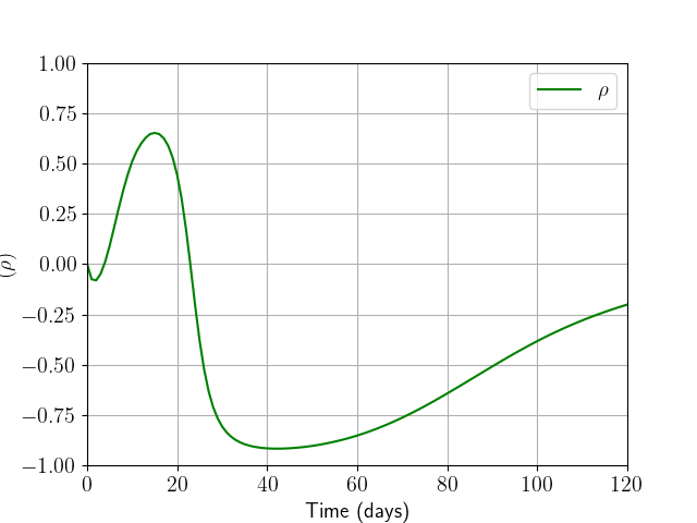
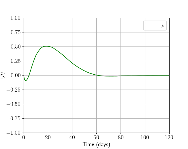
(d) Correlation coefficient

Figure 3: Sample paths of state components and correlation coefficient in the absence of control measures

To assess the impact of control measures, we simulate sample trajectories of the state dynamic for control measures fixed at moderate values, namely $(u^{L},u^{T},u^{V})=(0.2,0.03,0.015)$. Figure 4 depicts panels that are similar to those in Figure 3. we observe that as expected, the infection maximum is smaller compare to the case of no control measure. Additionally, more infectious people are detected and can be put in quarantine.

(a) All compartments

(b) Zoom in for small compartments

(c) Conditional covariance matrix entries

(d) Correlation coefficient

Figure 4: Sample paths of state components and correlation coefficient moderate control measures, $(u^{L},u^{T},u^{V})=(0.2,0.03,0.015)$

5.3 Results using state discretization, quantization and linear interpolation

The first numerical solution to our optimal control problem employs the backward recursion algorithm, approximating the conditional expectation through quantization and linear interpolation. Due to the computationally demanding aspect of our algorithm, we utilize the values in Table 3, for the number of discretization grid points for the state and control space. Even with this coarse discretization grid, the computational load is quite significant. Nevertheless, this grid yields already informative results for the value function and the optimal decision rule.

Discretization	Range		Values
Time step		$\Delta t$	1 day
Time horizon		$T=N_{t}\Delta t$	120 days
Quantization level		$N_{l}$	125
State   $M^{1}$	$[1,450]$	$\widetilde{N}_{1}$	6
State   $M^{2}$	$[1,450]$	$\widetilde{N}_{2}$	6
State   $Q^{1}$	$[1,1200]$	$\widetilde{N}_{3}$	6
State   $Q^{2}$	$[1,1200]$	$\widetilde{N}_{4}$	4
State   $\rho$	$[-0.5,0.5]$	$\widetilde{N}_{5}$	3
State   $Z^{1}$	$[1,350]$	$\widetilde{N}_{6}$	6
State   $Z^{2}$	$[1,990]$	$\widetilde{N}_{7}$	6
State   $Z^{3}$	$[1,50]$	$\widetilde{N}_{8}$	6
Control $u^{L}$	$[0,1]$	$\widetilde{N}^{L}$	6
Control $u^{T}$	$[0.001,0.07]$	$\widetilde{N}^{T}$	3
Control $u^{V}$	$[0,0.1]$	$\widetilde{N}^{V}$	3

Table 3: Table of discretization values

Remark 1

To apply the linear interpolation of the value function in dimension $8$, it is necessary to perform a Delaunay triangularization of the state space. Furthermore, this is followed by the computation of the location of the triangle in which each interpolant point belongs, as well as the calculation of the barycentric coordinates. Upon computing the value function with fewer grid points and for the model without the hospital, it was observed that the value function does not exhibit a direct dependence on the correlation coefficient between the two hidden states and the second diagonal entry of the conditional covariance matrix. In other words, when all the other variables are held constant, the value function shows to be independent on both $\rho$ and $Q^{2}$. This allows the curse of dimensionality to be alleviated by performing the linear interpolation in a six-dimensional subspace generated by the remaining state components, namely, $(M^{1},M^{2},Q^{1},Z^{1},Z^{2},Z^{3}).$ Another trick that we employed, due to the use of constant parameters, to reduce the computational time was to compute the search of triangles and the computation of barycentric coordinates for all the interpolants offline, prior to the backward recursion.

5.3.1 Value function and optimal decision rule as function of $(M^{1},Z^{1})$

The value function of our optimization problem is a function of eight variables, which presents a significant challenge in terms of visual representation. In order to gain insight into the behavior of this multi-variable function, it is necessary to make projections by setting specific values for certain variables. Since we are interested in an infectious disease, the two most important variables are the infection variables: the detected infected represented by $Z^{1}=I^{+}$ and the estimated number of undetected infected $M^{1}$. Hence, we visualize the value function and the optimal decision rule w.r.t. $M^{1},Z^{1}$ and the remaining variable are held constant. The two scenarios that we consider are: $(i)$ the case where all the other compartments are almost empty, except the susceptible $S$ that can be recovered by normalization, and $(ii)$ the case of other compartments with moderate sizes.

Small values of $(M^{2},Q^{1},Q^{2},\rho,Z^{2},Z^{3})$

This configuration may correspond to the early stage of the disease during which the majority of individuals have not yet recovered from the infection. It is therefore possible to represent the projected functions for a sample of time grid points. Typical behavior is observed at time steps $t=118$ days and $t=100$ days. In Figures 5, and 7, the remaining variables are set to small values as follows: $m^{2}=1,q^{1}=1,q^{2}=1,\rho=-0.5,z^{2}=1,z^{3}=1$.

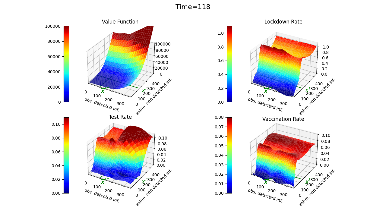
Figure 5: Linear interpolation method: value function and optimal decision rule at time $118$ for small values of $(m^{2},q^{1},q^{2},\rho,z^{2},z^{3})$

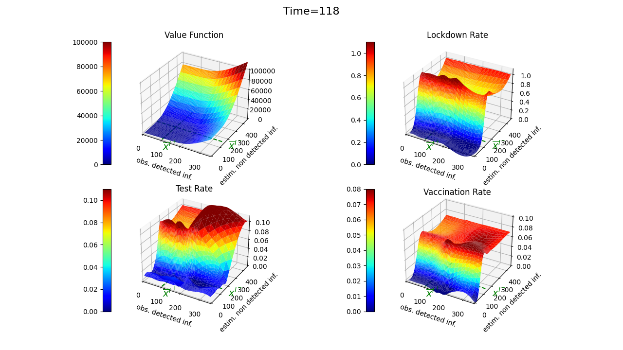
Figure 6: Regression method: value function and optimal decision rule at time $118$ for small values of $(m^{2},q^{1},q^{2},\rho,z^{2},z^{3})$

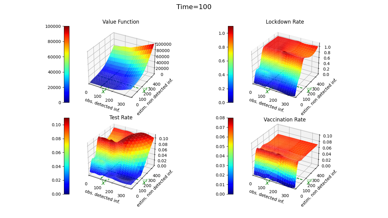
Figure 7: Linear interpolation method: value function and optimal decision rule at time $100$ for small values of $(m^{2},q^{1},q^{2},\rho,z^{2},z^{3})$

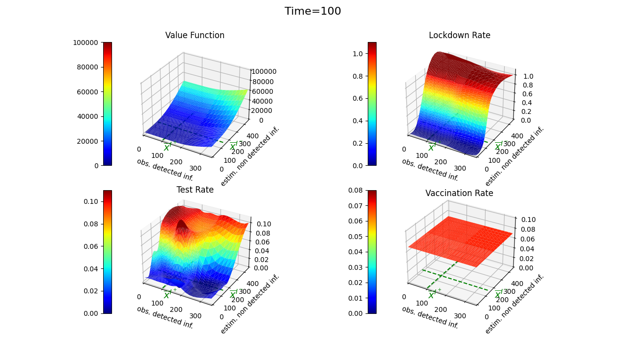
Figure 8: Regression method: value function and optimal decision rule at time $100$ for small values of $(m^{2},q^{1},q^{2},\rho,z^{2},z^{3})$

We note that on one hand, the value function as a function of $Z^{1}$ and $M^{1}$, inherits the linear and quadratic structure analogous to that observed in the running and terminal costs. The value function initially grows linearly for small values of $Z^{1}$ and the numbers of infected individuals increase and cross the respective thresholds, the growth becomes quadratic, which is a consequence of the quadratic structure of the penalty function. On the other hand, it is noteworthy that the optimal decision rule remains almost stationary up to 20 days before the time horizon, with only slight changes occurring as the terminal time approaches. In particular, the rate of lockdown appears to be largely independent of the number of detected infected individuals, with a significant dependence on the estimated number of undetected infectious cases. As a function of $M^{1}$, the lockdown rate evolves in a progressive manner, shifting from no social distancing when $M^{1}$ is small to a pronounced lockdown as the threshold $\overline{x}^{I^{-}}$ is exceeded. As with the lockdown rate, the test and vaccination rates are primarily contingent on the number of estimated undetected infectious cases, with a lesser dependence on $Z^{1}=I^{+}$. In addition, they both go from small detection and no vaccination rate when $M^{1}$ is negligible to being applied at maximum rate as $M^{1}$ approaches and crosses the threshold $\overline{x}^{I^{-}}$. In contrast to the gradual increase in the lock-down and testing rates, the vaccination rate rises rapidly to its maximum value. Consequently, the optimal decision rule is a combination of the three control variables, which are typically active at comparable levels. This indicates that, when necessary, intervention measures tend to combine the three controls to bring down the epidemic. This numerical result demonstrates that whenever the three control measures are available, it is advantageous to act simultaneously on all of them to mitigate the spread of the disease.

Moderate values of $(M^{2},Q^{1},Q^{2},\rho,Z^{2},Z^{3})$

To gain further insight into the value function and the optimal decision rule, we consider the remaining variables held fixed at moderate values: $m^{2}=100$, $q^{1}=500$, $q^{2}=500$, $\rho=0.5$, $z^{2}=200$, and $Z^{3}=30$. This setup represents the middle stage of the epidemic, with an estimated number of recovered individuals at $300$.

Figures 9 and 11 illustrate that the value function behaves similarly to the case with a fixed small compartment above, initially linear and then quadratic as it approaches the thresholds $\overline{x}^{I^{-}}$ and $\overline{x}^{I^{+}}$. The optimal decision rule primarily still depends on the estimated number of undetected infected individuals, $M^{1}$, shifting progressively from lower to higher control variable rates as $M^{1}$ approaches and exceeds the threshold $\overline{x}^{I^{-}}$.

Meanwhile, when both $I^{+}$ and $M^{1}$ exceed their respective thresholds, the rates for lockdown and vaccination decline, while the testing rate remains high. This indicates that, in a scenario where a moderate number of individuals have already recovered (being in either compartment $R^{+}$ or $R^{-}$) and the sizes of infected compartments $I^{-}$ and $I^{+}$ have surpassed their thresholds, it becomes unnecessary to apply lockdown and vaccination measures since almost no one is susceptible anymore.

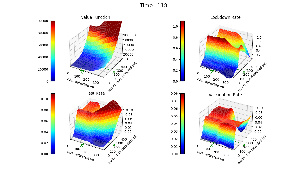
Figure 9: Linear interpolation method: value function and optimal decision rule at time $118$ for moderate values of $(m^{2},q^{1},q^{2},\rho,z^{2},z^{3})$

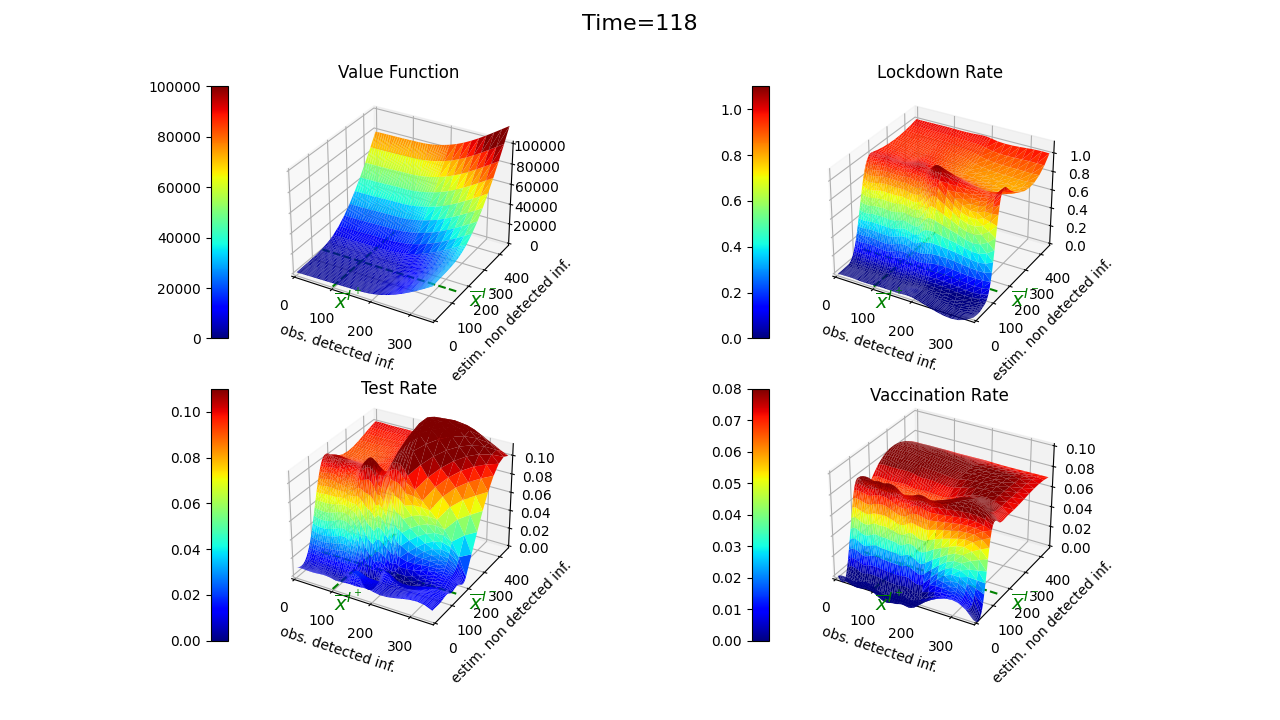
Figure 10: Regression method: value function and optimal decision rule at time $118$ for moderate values of $(m^{2},q^{1},q^{2},\rho,z^{2},z^{3})$

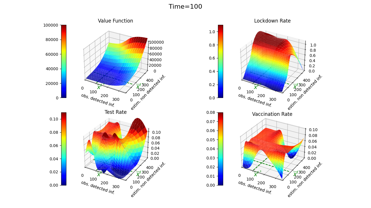
Figure 11: Linear interpolation method: value function and optimal decision rule at time $100$ for moderate values of $(m^{2},q^{1},q^{2},\rho,z^{2},z^{3})$

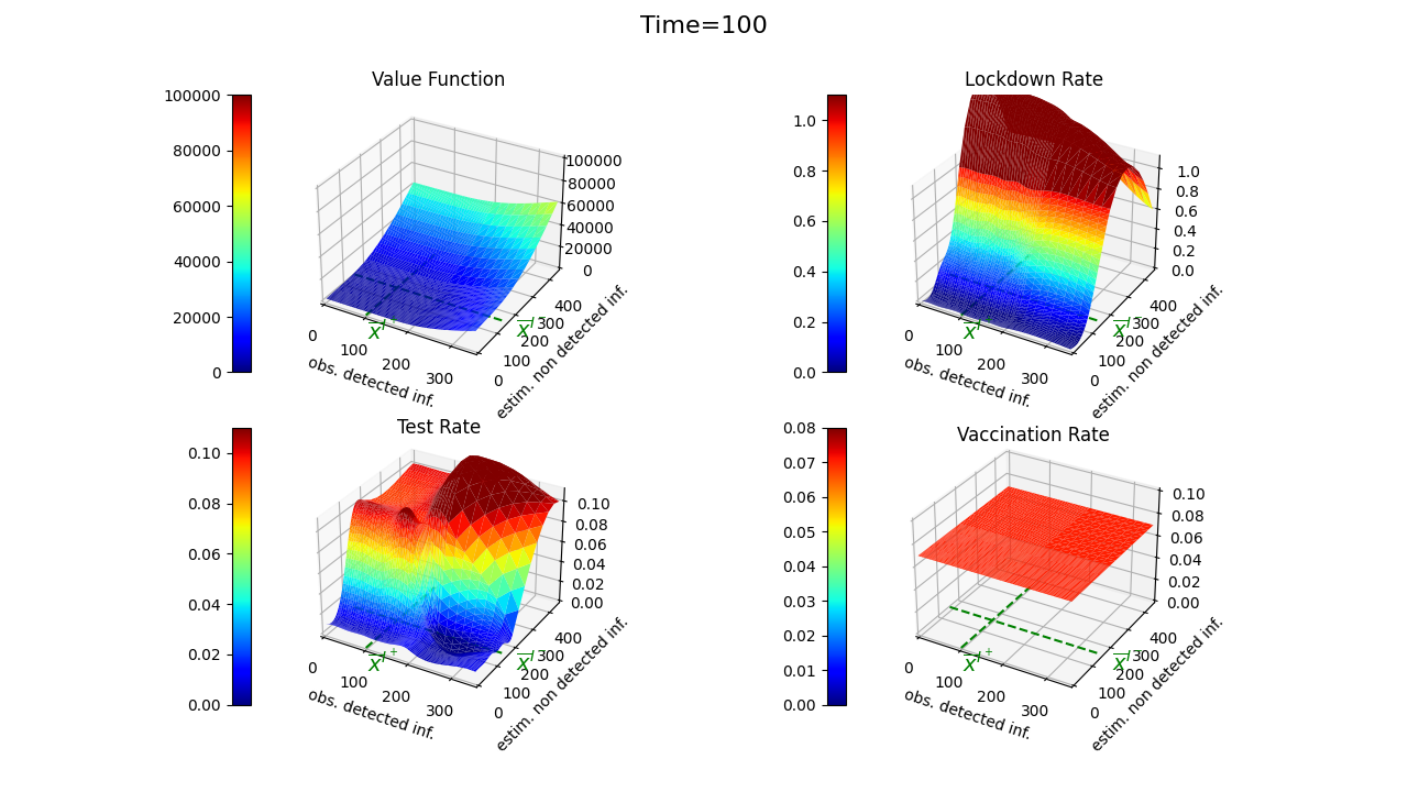
Figure 12: Regression method: value function and optimal decision rule at time $100$ for moderate values of $(m^{2},q^{1},q^{2},\rho,z^{2},z^{3})$

5.3.2 Optimal path of the epidemic state process

With the knowledge of the optimal decision rule at all grid points of the state space, we can simulate an optimal sample path of the state process using the optimal control of the nearest neighbor projection. Figures 13 and 15 illustrate the dynamics of sample compartment sizes and the dynamics of the applied control measures. We observe that the infection compartment sizes, $I^{+}$ and the estimate of $I^{-}$, are driven quickly toward zero in approximately 25 to 30 days. Meanwhile, the estimates of compartment sizes $S$ and $R^{-}$ decrease and stabilize once there are no more infected individuals in the population. The hospital compartment size fluctuates slightly but remains low and below the hospital threshold throughout the infection period, unlike the benchmark scenario where the threshold was exceeded. Regarding the optimal control measures, we see that initially, a strong lockdown is applied along with significant levels of testing and vaccination. The lockdown is gradually eased after one week, while testing and vaccination continue. Approximately one week after the end of the lockdown, testing is stopped, and only vaccination continues for approximately two more weeks.

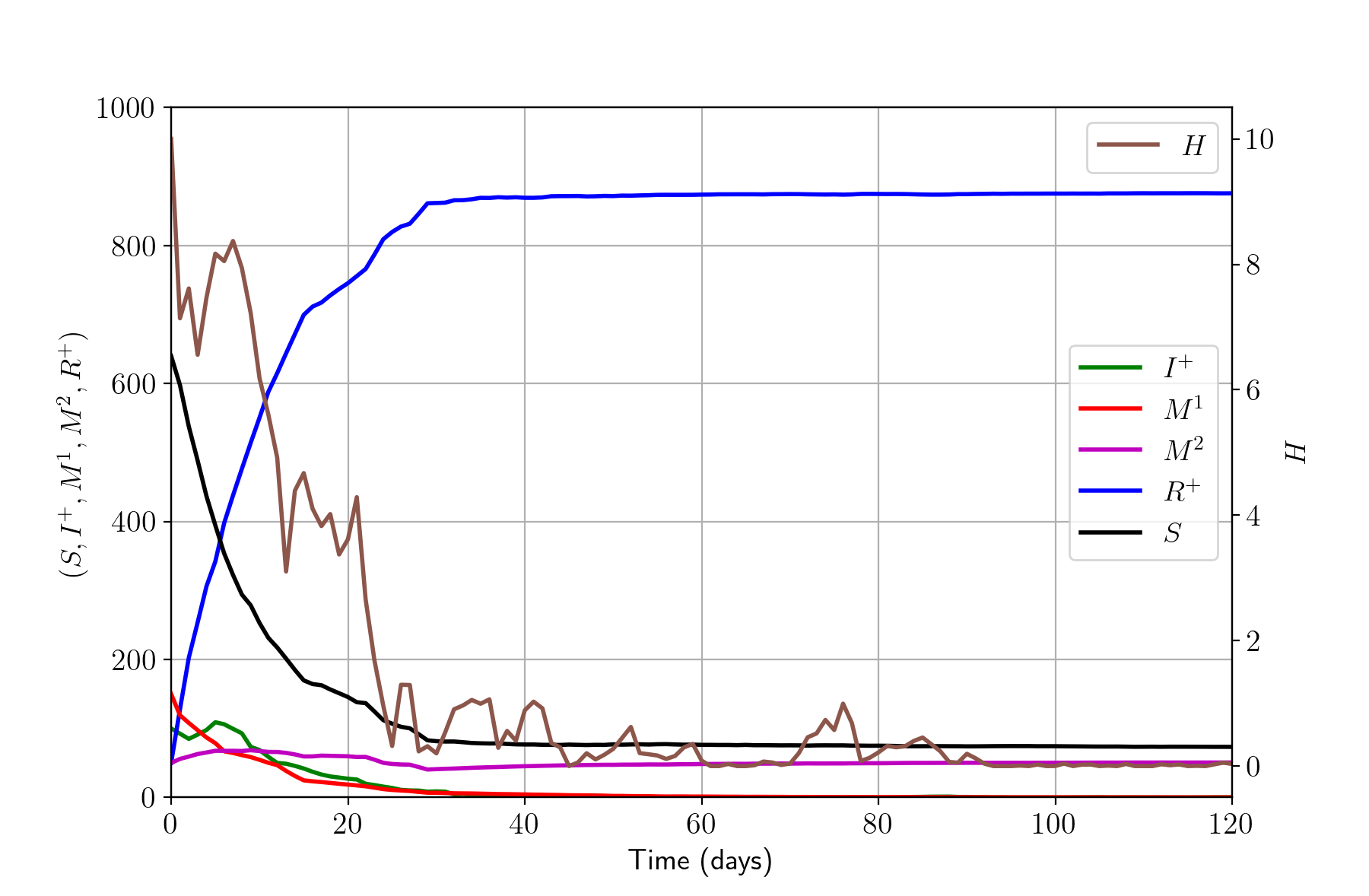
Figure 13: Linear interpolation method: optimal trajectories of compartments size ; Initial state is $m^{1}=150,m^{2}=50,q^{1}=200,q^{2}=200,\rho=0,z^{1}=100,z^{2}=50,z^{3}=10$; The hospital y-axis is on the right-hand side and the y-axis of the rest is on the left.

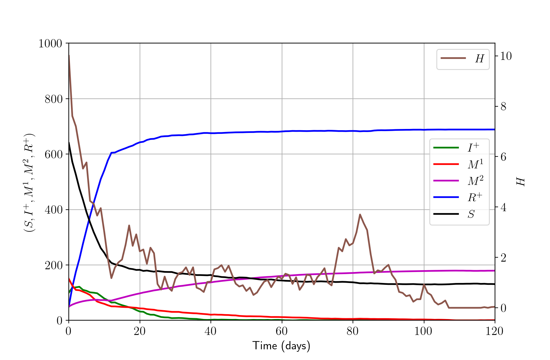
Figure 14: Regression method: Optimal compartment size path ; Initial state: $(m^{1}=150,m^{2}=50,q^{1}=200,q^{2}=200,\rho=0,z^{1}=100,z^{2}=50,z^{3}=10$); The hospital y-axis is on the right-hand side and the y-axis of the rest is on the right

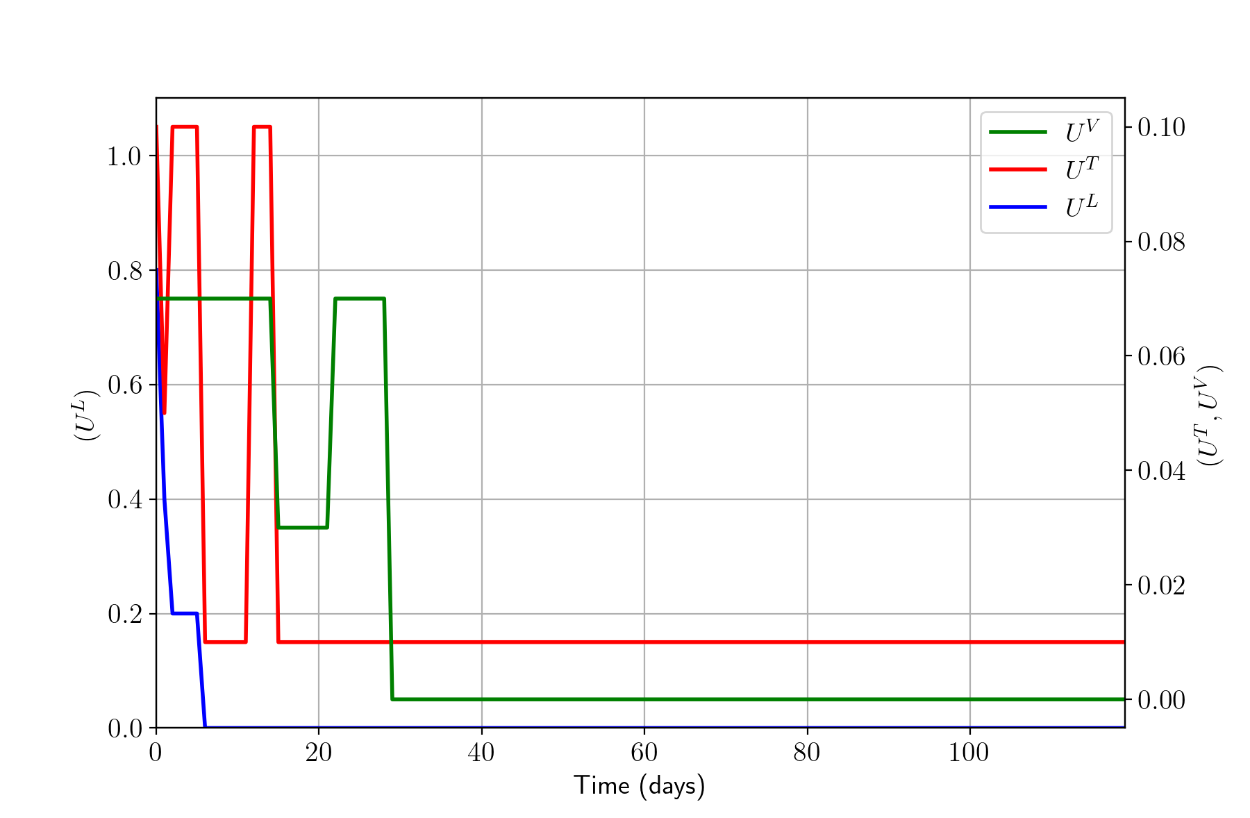
Figure 15: Linear interpolation method: optimal policy ; Initial state is $m^{1}=150,m^{2}=50,q^{1}=200,q^{2}=200,\rho=0,z^{1}=100,z^{2}=50,z^{3}=10$; The $u^{L}$ y-axis is on the left-hand side and the y-axis of $U^{T},U^{V}$ is on the right.

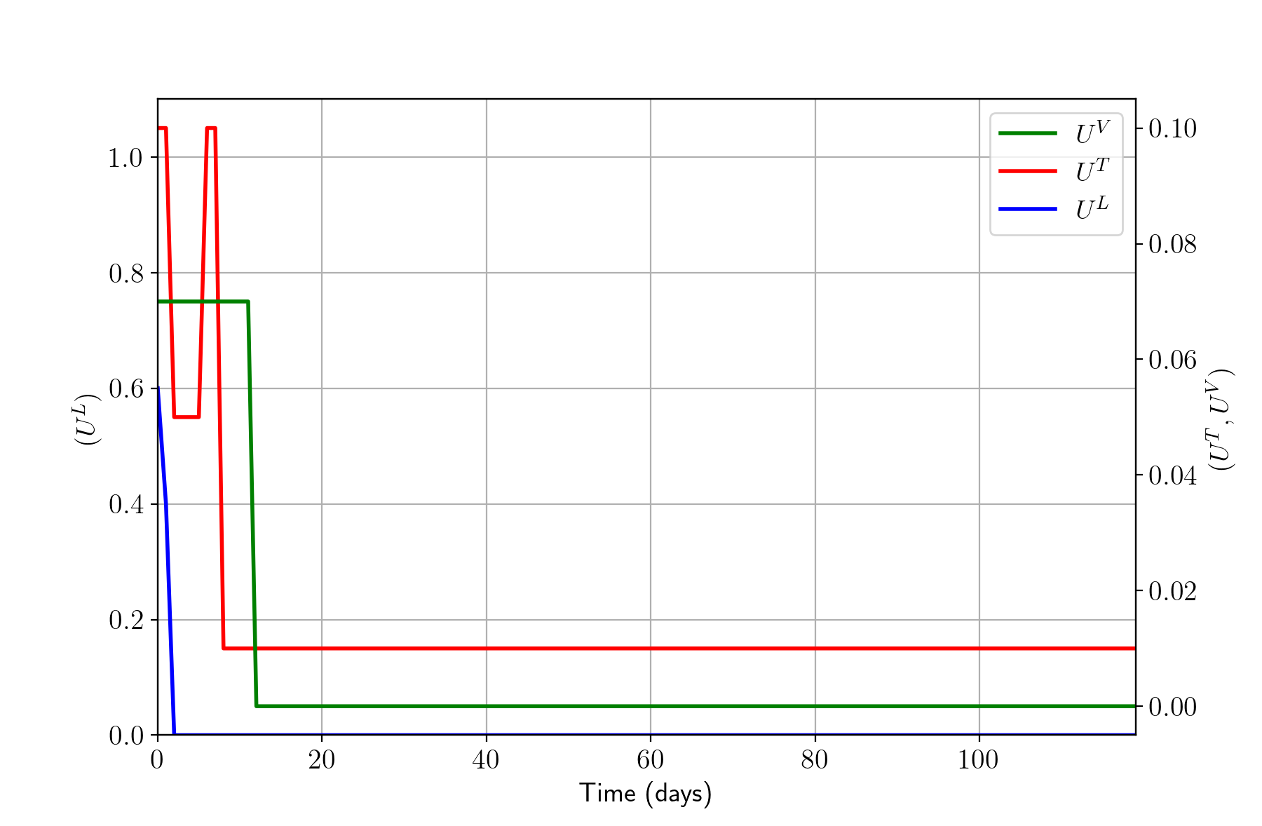
Figure 16: Regression method: optimal control path; Initial state: $(m^{1}=150,m^{2}=50,q^{1}=200,q^{2}=200,\rho=0,z^{1}=100,z^{2}=50,z^{3}=10$); The $u^{L}$ y-axis is on the left-hand side and the y-axis of $U^{T},U^{V}$ is on the right.

5.4 Numerical results using state discretization, quantization and value function regression

In this section, we present the numerical results obtained through our second approach: value function regression. This method involves selecting a set of ansatz functions for the least squares regression. Leveraging our previous results obtained via linear interpolation, which provided insights into the behavior of the value function with respect to each component of the state process, we consider the following functions defined for $x=(m^{1},m^{2},q^{1},q^{2},q^{12},z^{1},z^{2},z^{3})$,

• constant function:        $\varphi_{0}(x)~~=c$;

• Linear functions:        $\varphi_{1}(x)$ $=$ $z^{1}$; $\varphi_{4}(x)$ $=$ $m^{1}$; $\varphi_{2}(x)$ $=$ $z^{2}$; $\varphi_{5}(x)$ $=$ $m^{2}$; $\varphi_{3}(x)$ $=$ $z^{3}$; $\varphi_{6}(x)$ $=$ $q^{1}$.

• Quadratic functions: $\varphi_{7}(x)$ $=$ $\max(z^{1}-\overline{\text{x}}^{I^{+}},0)^{2}$; $\varphi_{8}(x)$ $=$ $\max(m^{1}-\overline{\text{x}}^{I^{-}},0)^{2}$; $\varphi_{9}(x)$ $=$ $\max(N-z^{1}-z^{2}-z^{3}-\overline{\text{x}}^{\text{Test}},0)^{2}$ $=$ $\max(\text{x}^{\text{Test}}-\overline{\text{x}}^{\text{Test}},0)^{2}$; $\varphi_{10}(x)$ $=$ $\max(N-z^{1}-z^{2}-z^{3}-\overline{\text{x}}^{\text{Vacc}},0)^{2}$ $=$ $\max(\text{x}^{\text{Test}}-\overline{\text{x}}^{\text{Vacc}},0)^{2}$; $\varphi_{11}(x)$ $=$ $(N-z^{1})^{2}~=~(\text{x}^{\text{work}})^{2}$ ; $\varphi_{12}(x)$ $=$ $\max(z^{3}-\overline{\text{x}}^{H},0)^{2}$

• Function appearing in the infection cost for non-detected infectious:

  $\varphi_{13}(x)$$=$ $\big{(}(m^{1}-\overline{\text{x}}^{I^{-}})^{2}+q^{1}\big{)}\Phi_{\pazocal{N}}\Big{(}\dfrac{m^{1}-\overline{\text{x}}^{I^{-}}}{\sqrt{q^{1}}}\Big{)}+(m^{1}-\overline{\text{x}}^{I^{-}})\sqrt{\dfrac{q^{1}}{2\pi}}\exp\Big{(}-\frac{1}{2}\dfrac{(m^{1}-\overline{\text{x}}^{I^{-}})^{2}}{q^{1}}\Big{)};$

  where $\Phi_{\pazocal{N}}$ is the cumulative distribution function of the standard normal distribution.

Each of these functions is either of the form of a function appearing in the running or terminal cost, or follows the shape observed from the linear interpolation results. It is important to note that for the value function at terminal time, we know exactly the structure of the value function.

To ensure a fair comparison between results from both methods, we use the same set of parameters and discretization grid points as in the first approach.

5.4.1 Value function and optimal decision rule w.r.t. $M^{1},Z^{1}$

Similar to the first method we visualize the value function and optimal decision rule w.r.t. the two infection compartments. Once again, we consider scenarios of remaining compartments held fixed to small and moderate sizes as previously. Figures 6, 8, 10, and 12 display the value function and optimal decision in configurations identical to those used in the linear interpolation approach. Overall, the results from both methods appear consistent, especially both optimal decision rules seem to exhibit a generally similar structure. However, it should firstly be noted that the optimal decision rule is smoother for the approach with value function regression. This is certainly due to the constraint of the value function to belong to the vector space of functions generated by the chosen basis of ansatz functions. Secondly, the optimal decision rules obtained with regression do not capture well all the nuances observed at the boundaries in the linear interpolation method results. For instance, comparing the optimal decision rules in Figures 9, 11 and 10, 12, we observe in the result with linear interpolation that as both the number of detected infected $Z^{1}$ and the estimated number of non-detected infected $M^{1}$ are greater than their respective thresholds, the optimal decision rule suggests dropping the lockdown and vaccination measures and maintaining only the maximum possible level of testing. Conversely, the linear regression result indicates maintaining all the three control measures at high levels, with only the lockdown rate that drop slightly at time step $t=100$ days. Thirdly, the value function obtained through regression seems to underestimate that derived from linear interpolation. This is illustrated in the value functions at time step $t=100$ days (Figures 7, 11 and 8 12), where in the case of linear interpolation the maximum values is greater than $100,000$ monetary unit, while in the regression case, the maximum value is around $60,000$ monetary unit.

5.4.2 Optimal path of the epidemic state process

The optimal decision rule derived from value function regression can then be used to simulate the optimal dynamics of the epidemic. Figures 14 and 16 depict sample path of compartment sizes and the optimal control measures to be applied, respectively. These figures show that the number of infected individuals decreases progressively to zero within $80$ days. The implemented control strategy involves an early strong lockdown lasting only a few days, coupled with vaccination for nearly $15$ days and less than $10$ days of testing. After $15$ days, all the control measures are lifted and only the minimal possible testing continues. Compared to the optimal strategy derived from the linear interpolation method, the strategy obtained through regression takes a relatively longer period to reduce the number of infected individuals to zero. This is understandable, as restricting the form of the value function results in a suboptimal strategy. However, this suboptimal strategy effectively keeps the hospital compartment size quite small and below the threshold capacity throughout the infection period.

Acknowledgments  The authors thank Olivier Menoukeu Pamen (University of Liverpool), Gerd Wachsmuth, Armin Fügenschuh, Markus Friedemann, Jesse Beisegel (BTU Cottbus–Senftenberg) for insightful discussions and valuable suggestions that improved this paper.

Funding  The authors gratefully acknowledge the support by the Deutsche Forschungsgemeinschaft (DFG), award number 458468407, and by the German Academic Exchange Service (DAAD), award number 57417894.

Appendix

Appendix A Proofs

Proof (Proposition 2)

Let us denote by $\pazocal{F}^{Z}_{0}=\pazocal{F}^{I}_{0}v\sigma\{Z_{0}\}$ the initial information $\sigma$-algebra generated by the initial guess of $Y_{0}$ and the initial observation $Z_{0}$. We recall that the conditional distribution of $Y(0)$ follows a Gaussian law $\pazocal{N}(m_{0},q_{0})$.

Taking the conditional expectation of the performance criterion with respect to the initial information $\pazocal{F}^{Z}_{0}$, we obtain

$$\mathbb{E}[\pazocal{J}^{F}(X_{0},u)|\pazocal{F}^{Z}_{0}] = \mathbb{E}\Big{[}\sum_{n=0}^{N_{t}-1}\hskip 9.00002pt\Psi^{F}((Y_{n},Z_{n}),u_{n})\hskip 18.00003pt+\hskip 13.50002pt\Phi^{F}(Y_{N_{t}},Z_{N_{t}})\Big{|}\pazocal{F}^{Z}_{0}\Big{]}$$

$$\displaystyle= \displaystyle\mathbb{E}\Big{[}\sum_{n=0}^{N_{t}-1}\mathbb{E}\Big{[}\Psi^{F}((Y_{n},Z_{n}),u_{n})\Big{|}\pazocal{F}_{n}^{Z}\Big{]}+\mathbb{E}\Big{[}\Phi^{F}(Y_{N_{t}},Z_{N_{t}})\Big{|}\pazocal{F}_{N_{t}}^{Z}\Big{]}\Big{|}\pazocal{F}^{Z}_{0}\Big{]}$$

This last equality is obtained using the tower low of conditional expectation since $\pazocal{F}_{0}^{Z}\subseteq\pazocal{F}_{n}^{Z}$ for all $n\geq 0$. Then, because $\Psi^{F}$ and $\Phi^{F}$ are considered linear and quadratic in $y$, the above conditional expectation $\mathbb{E}[\ldots|\pazocal{F}_{n}^{Z}]$, $n=0,\cdots,N_{t}$ can be expressed in terms of the extended Kalman filter $(M,Q)$ approximation for the hidden state $Y$. We recall that in the case of conditionally Gaussian sequences treated in Liptser and Shiryaev (2013), the conditional distribution of $Y_{n}$ is the Gauss distribution $\pazocal{N}(M_{n},Q_{n})$. When computing the conditional expectation of running and terminal costs, expression that are fully observable, meaning that they do not depend on the hidden state $Y$, are not modified. In our case, it means that only the running and terminal infection costs for non-detected infectious are modified (since $X^{\text{Work}}=N-Z^{1}$ and $X^{\text{Test}}=N-(Z^{1}+Z^{2}+Z^{3})$ allow to obtain fully observable expressions for economic, detection and vaccination costs). The running infection costs for non-detected infectious becomes

$$\mathbb{E}\Big{[}C^{-}_{I}\left(Y^{1}_{n},\overline{\text{x}}^{I^{-}}\right)\Big{|}\pazocal{F}_{n}^{Z}\Big{]} = \mathbb{E}\Big{[}a_{I^{-}}Y^{1}_{n}+b_{I^{-}}(Y^{1}_{n}-\overline{\text{x}}^{I^{-}})_{+}^{2}\Big{|}\pazocal{F}_{n}^{Z}\Big{]}$$

$$= a_{I^{-}}M^{1}_{n}+b_{I^{-}}\mathbb{E}\Big{[}(Y^{1}_{n}-\overline{\text{x}}^{I^{-}})_{+}^{2}\Big{|}\pazocal{F}_{n}^{Z}\Big{]}.$$

Further, because the conditional law of $Y^{1}_{n}$ given $\pazocal{F}_{n}^{Z}$ is Gaussian with mean $M^{1}_{n}$ and variance $Q^{1}_{n}$, we have,

$$\mathbb{E}\Big{[}C^{-}_{I}\left(Y^{1}_{n},\overline{\text{x}}^{I^{-}}\right)\Big{|}\pazocal{F}_{n}^{Z}\Big{]} = a_{I^{-}}M^{1}_{n}+b_{I^{-}}\int_{\overline{\text{x}}^{I^{-}}}^{\infty}(y-\overline{\text{x}}^{I^{-}})^{2}\dfrac{1}{\sqrt{2\pi Q^{1}_{n}}}\exp\Big{(}-\frac{1}{2}\dfrac{(y-M^{1}_{n})^{2}}{Q^{1}_{n}}\Big{)}dy.$$

Similar expressions are derived for the terminal infection costs for non-detected infectious.

Hence, there exist measurable functions $\Psi$ and $\Phi$ as given in the proposition, such that

$$\mathbb{E}[\pazocal{J}^{F}(X_{0},u)|\pazocal{F}^{Z}_{0}]=\displaystyle\mathbb{E}_{m_{0},q_{0},z}\Big{[}\sum_{n=0}^{N_{t}-1}\Psi(M_{n},Q_{n},Z_{n},u_{n})+\Phi(M_{N_{t}},Q_{N_{t}},Z_{N_{t}})\Big{]}\\$$

∎

Proof (Lemma 1 )

The transformation of this integral is done by two successive changes of variable. First, let $\widetilde{y}=y-\overline{\text{x}}^{I^{-}}$, thus the integral becomes
$\displaystyle\int_{0}^{\infty}\widetilde{y}^{2}\dfrac{1}{\sqrt{2\pi q^{1}}}\exp\Big{(}-\frac{1}{2}\dfrac{(\widetilde{y}+\overline{\text{x}}^{I^{-}}-m^{1})^{2}}{q^{1}}\Big{)}d\widetilde{y}$. Second, let $\widehat{m}=m^{1}-\overline{\text{x}}^{I^{-}}$ and $\widehat{y}=\dfrac{\widetilde{y}-\widehat{m}}{\sqrt{q^{1}}}$, we deduce that the integral reads

$\displaystyle\int_{-\dfrac{\widehat{m}}{\sqrt{q^{1}}}}^{\infty}(\widehat{m}+\sqrt{q^{1}}\widehat{y})^{2}\dfrac{1}{\sqrt{2\pi}}\exp\Big{(}-\frac{1}{2}\widehat{y}^{2}\Big{)}d\widehat{y}$.

After expansion of the quadratic term in the integral and identification of the cumulative distribution function of the standard normal distribution
$\Phi_{\pazocal{N}}(t)=\displaystyle\int_{-\infty}^{t}\dfrac{1}{\sqrt{2\pi}}\exp(-\dfrac{1}{2}\widehat{y}^{2})d\widehat{y}$, we obtain the result
$\big{(}(m^{1}-\overline{\text{x}}^{I^{-}})^{2}+q^{1}\big{)}\Phi_{\pazocal{N}}\Big{(}\dfrac{m^{1}-\overline{\text{x}}^{I^{-}}}{\sqrt{q^{1}}}\Big{)}+(m^{1}-\overline{\text{x}}^{I^{-}})\sqrt{\dfrac{q^{1}}{2\pi}}\exp\Big{(}-\frac{1}{2}\dfrac{(m^{1}-\overline{\text{x}}^{I^{-}})^{2}}{q^{1}}\Big{)}.$

Appendix B Transition operator functions

Expressions of functions involved in the transition operators are:

$$f_{M}(n,m,q,z,\nu)= m+f(n,m,z),$$

$$f_{Q}(n,m,q,z,\nu)= -\left[g\ell^{\top}+f_{1}qh_{1}^{\top}\right]\left[\ell\ell^{\top}+h_{1}qh_{1}^{\top}\right]^{+}\left[g\ell^{\top}+f_{1}qh_{1}^{\top}\right]^{\top}+f_{1}qf_{1}^{\top}+\sigma\sigma^{\top},$$

$$f_{Z}(n,m,q,z,\nu)= h_{0}+h_{1}m,$$

$$g_{M}(n,m,q,z,\nu)= \left[g\ell^{\top}+f_{1}qh_{1}^{\top}\right]\Big{(}\left[\ell\ell^{\top}+h_{1}qh_{1}^{\top}\right]^{+}\Big{)}^{\frac{1}{2}},$$

$$g_{Z}(n,m,q,z,\nu)= \left[\ell\ell^{\top}+h_{1}qh_{1}^{\top}\right]^{1/2}.$$

Appendix C Additional numerical results

C.1 Value function obtained with interpolation method w.r.t. each component of the state process

To better understand how the value function evolves with respect to each component of the state process, we freeze all variables except one and represent the value function in terms of that single variable. This approach is particularly helpful in determining the form of the ansatz function required for the second numerical approach, which involves fitting the value function. Therefore, the other components are fixed at either small or moderate values while the value function is plotted against the component of interest. Figures 17( Panels 17(a),17(c),17(e)), 18 ( Panels 18(a),18(c),18(e)), 19( Panels 19(a),19(c),19(e)), and 20 ( Panels 20(a),20(c),20(e)) illustrate the shape of the value function depending on these components. We observe that the value function has a linear plus quadratic shape with respect to components $Z^{1}$, $Z^{3}$, and $M^{1}$. Additionally, it exhibits a decreasing shape as a function of $Z^{2}=R^{+}$ and $M^{2}$. Finally, the value function appears as a linearly increasing function with respect to the first diagonal entry of the conditional covariance $Q^{1}$. This can be explained by the fact that as $Q^{1}$ increases, there is more uncertainty in the estimate of $M^{1}$, suggesting that higher values of $M^{1}$ are more likely and come with higher costs.

Interpolation                 Regression

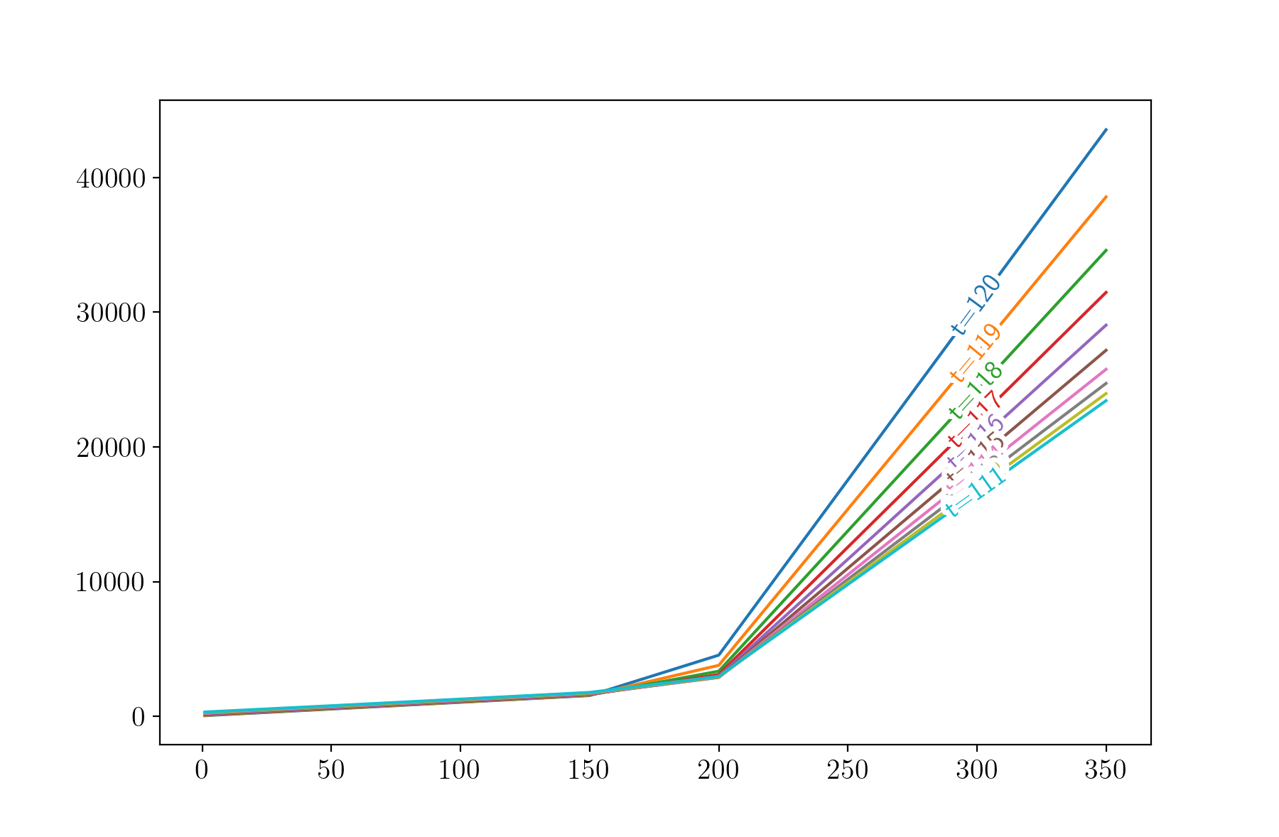
(a) Function of $z^{1}$, other variables small

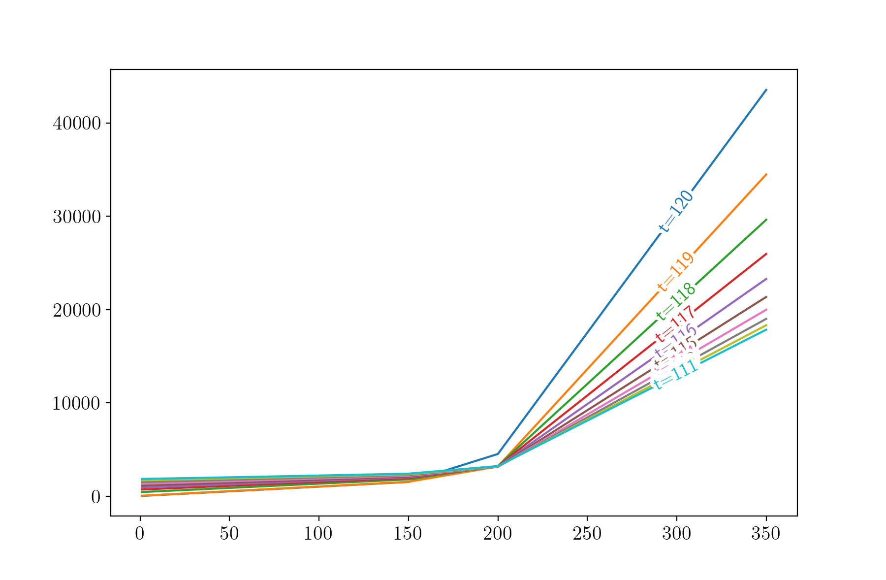
(b) Function of $z^{1}$, other variables small

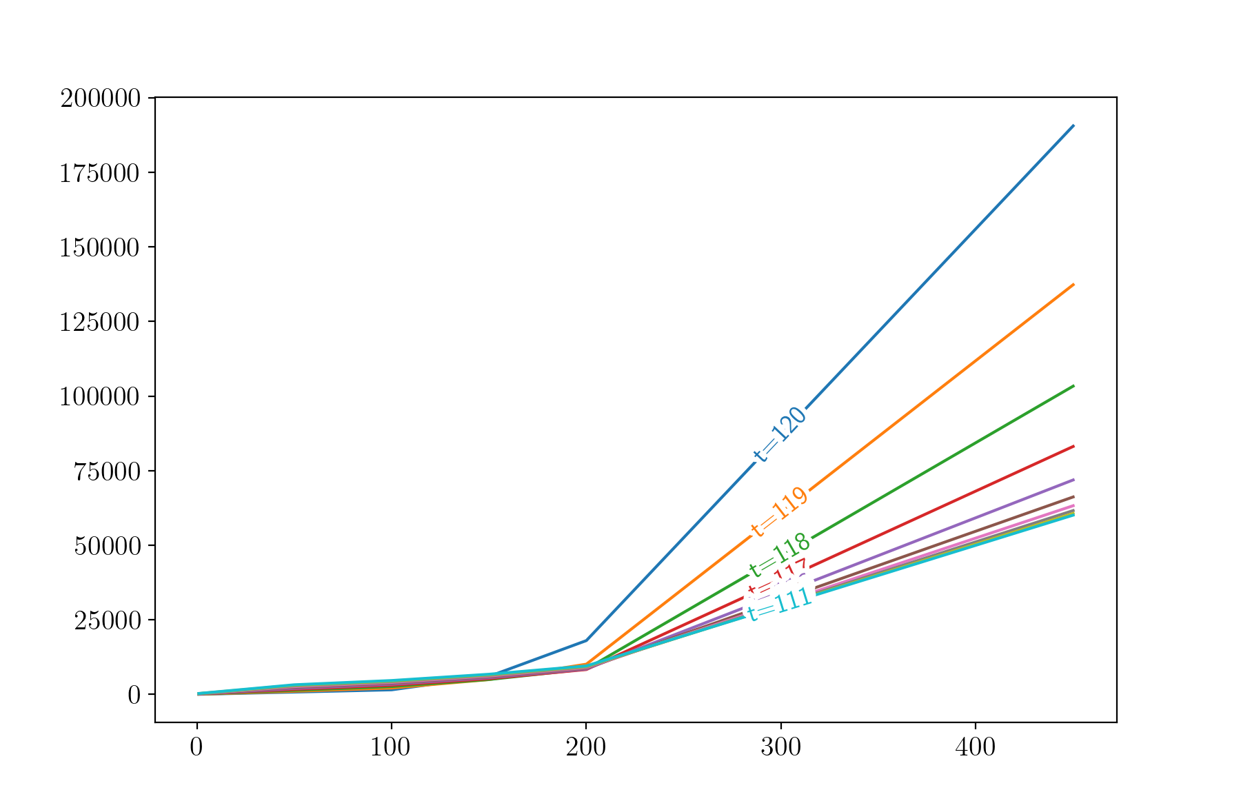
(c) Function of $m^{1}$, other variables small

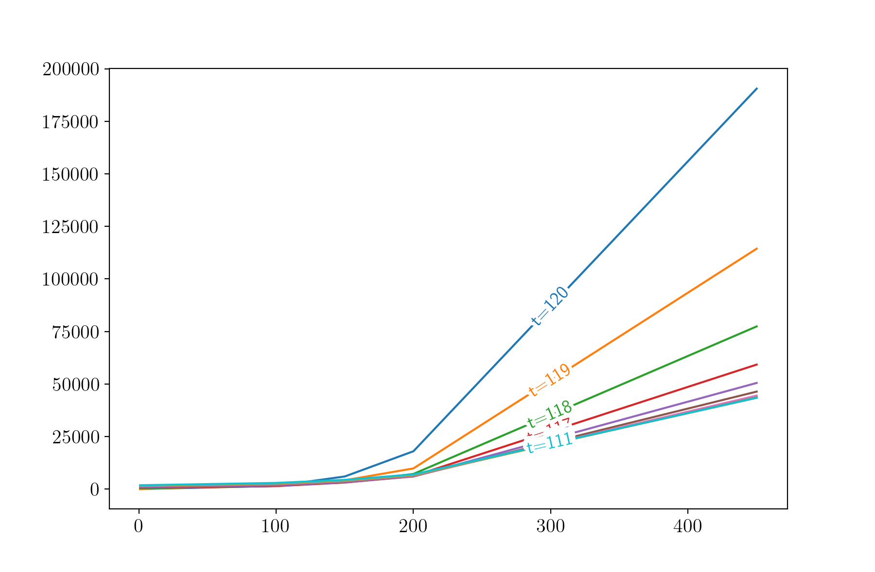
(d) Function of $m^{1}$, other variables small

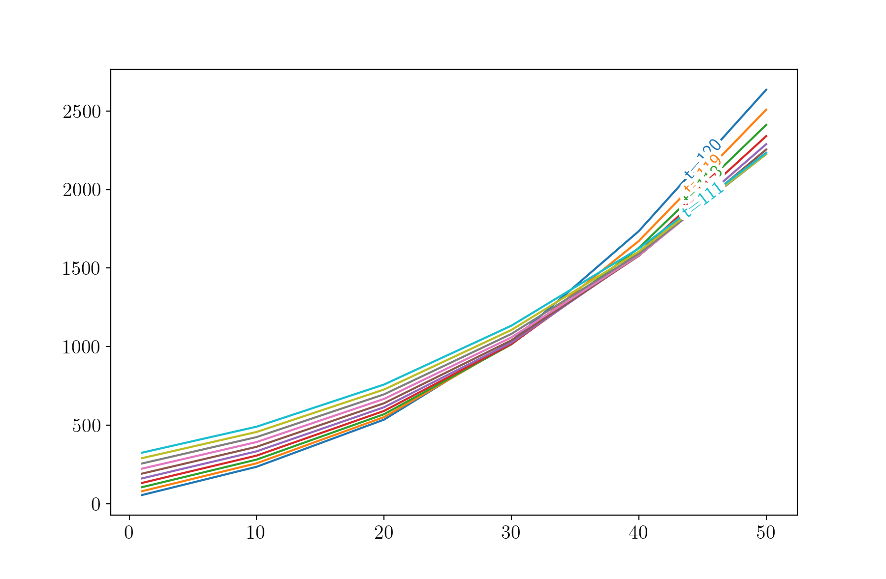
(e) Function of $z^{3}$, other variables small

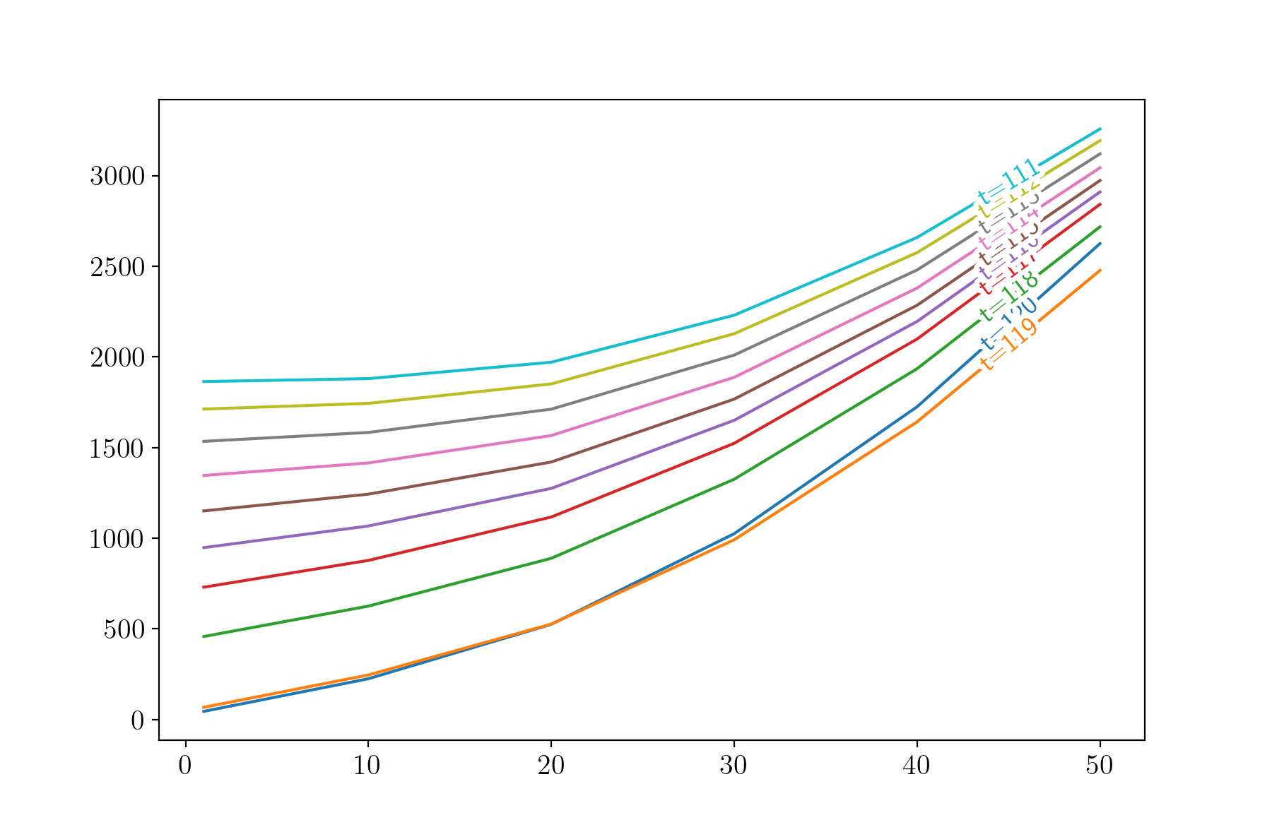
(f) Function of $z^{3}$, other variables small

Figure 17: Value function from linear interpolation approach (left) and regression approach
(right) as function of $z^{1}$, $m^{1}$ and $z^{3}$

Interpolation                 Regression

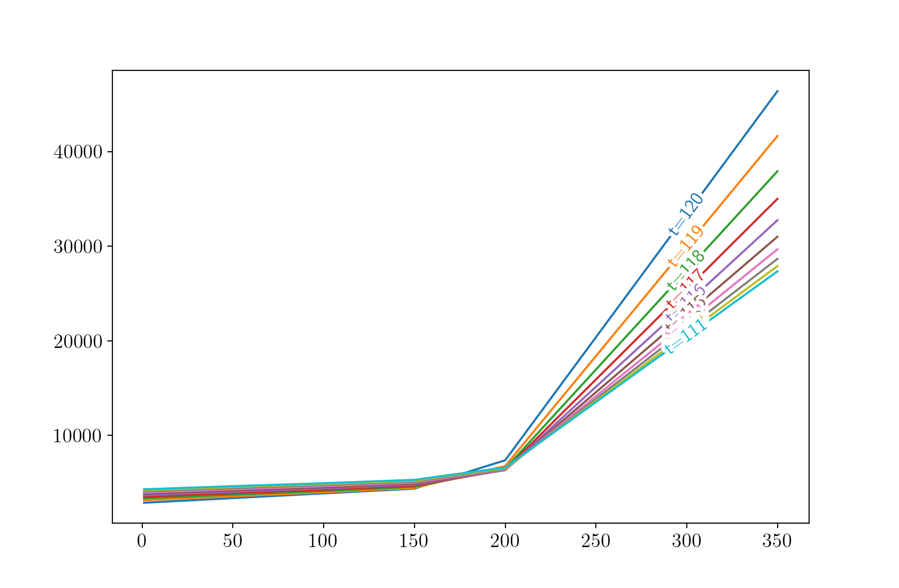
(a) Function of $z^{1}$, other variables moderate

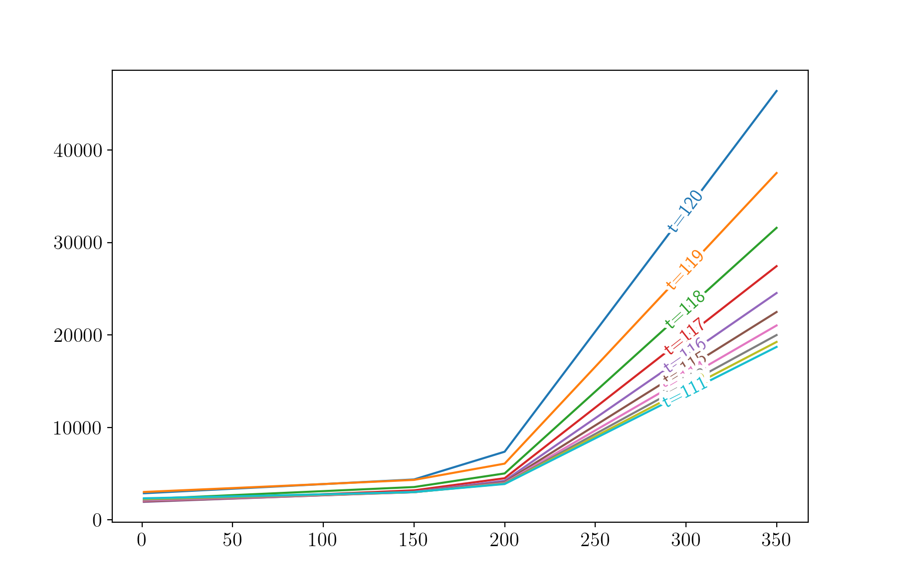
(b) Function of $z^{1}$, other variables moderate

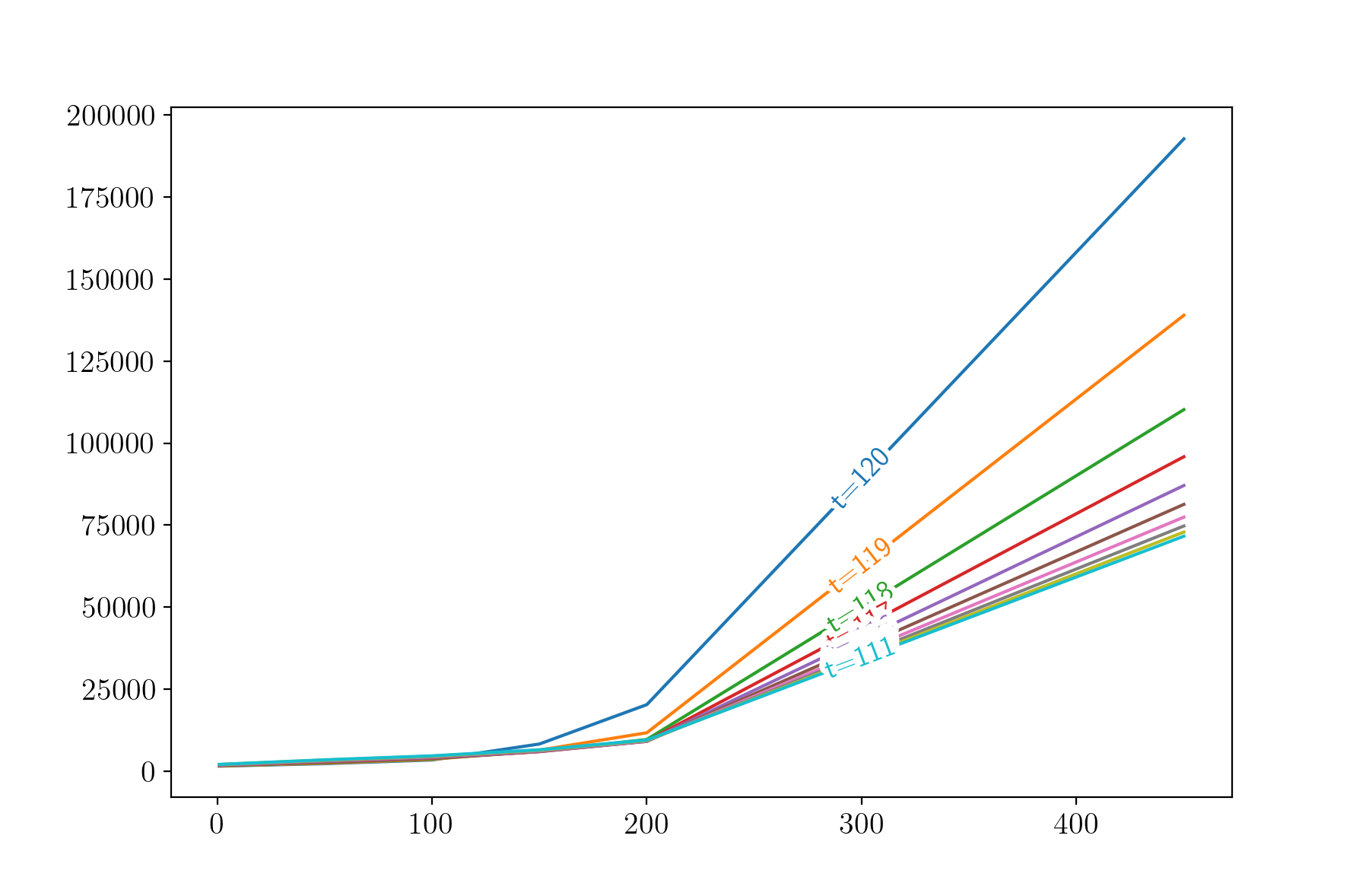
(c) Function of $m^{1}$, other variables moderate

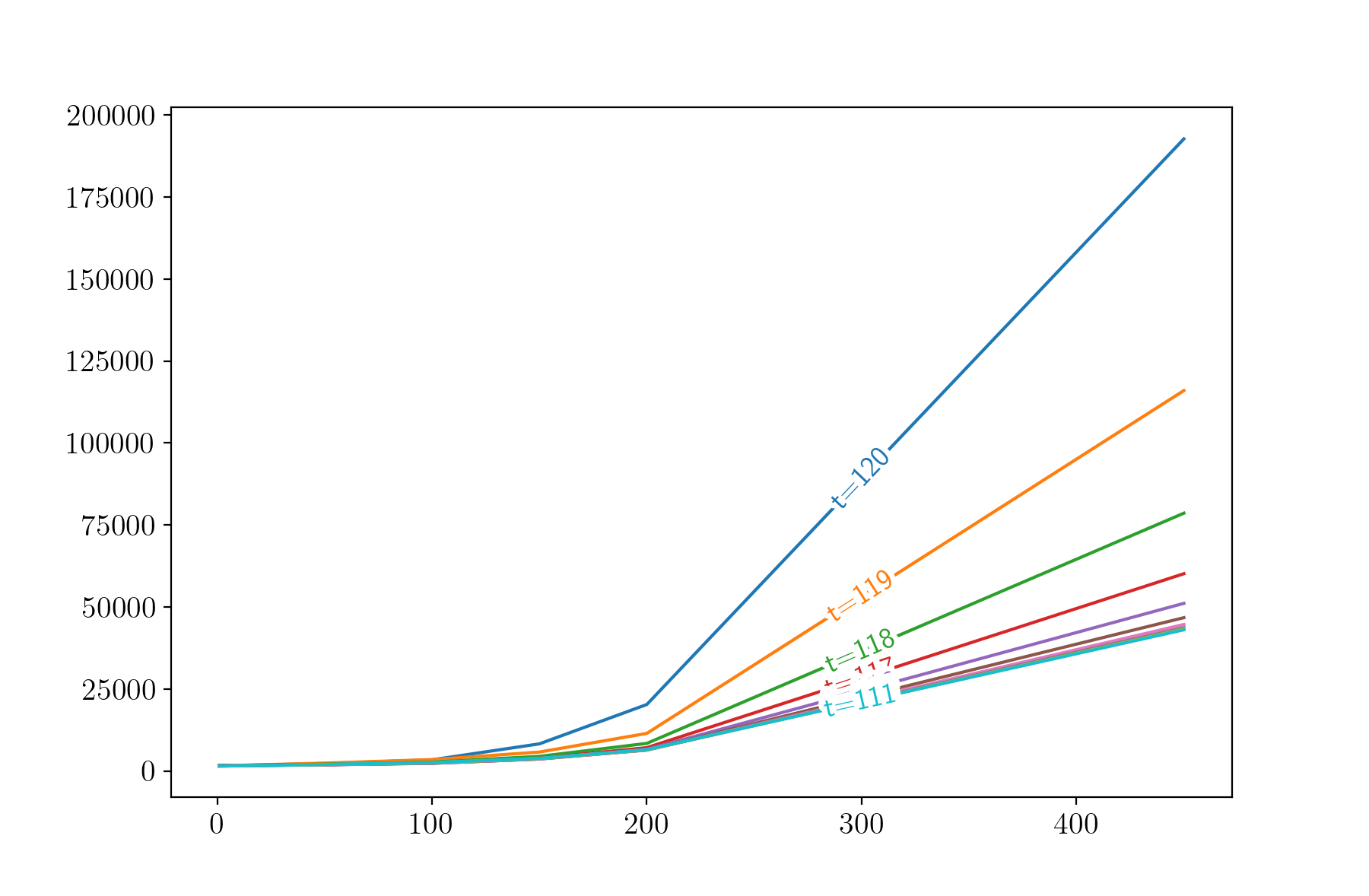
(d) Function of $m^{1}$, other variables moderate

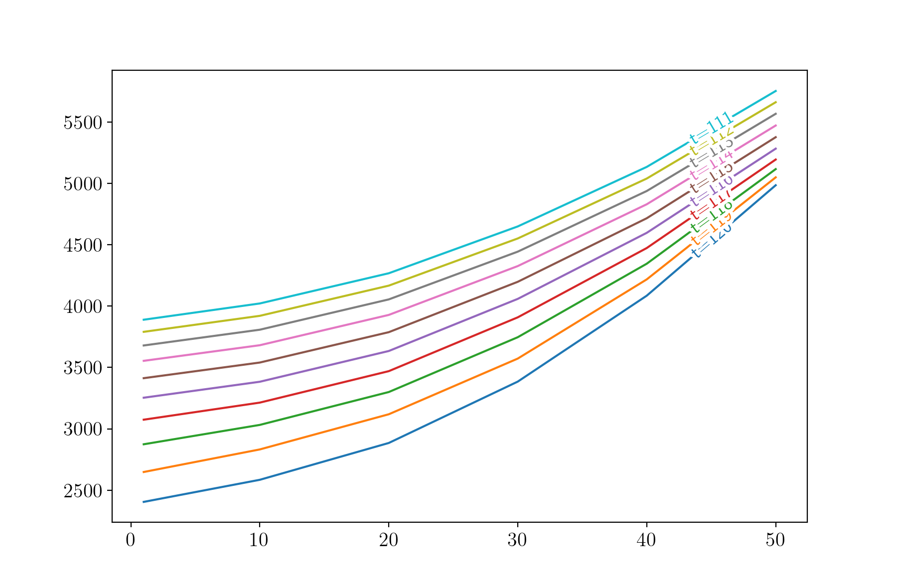
(e) Function of $z^{3}$, other variables moderate

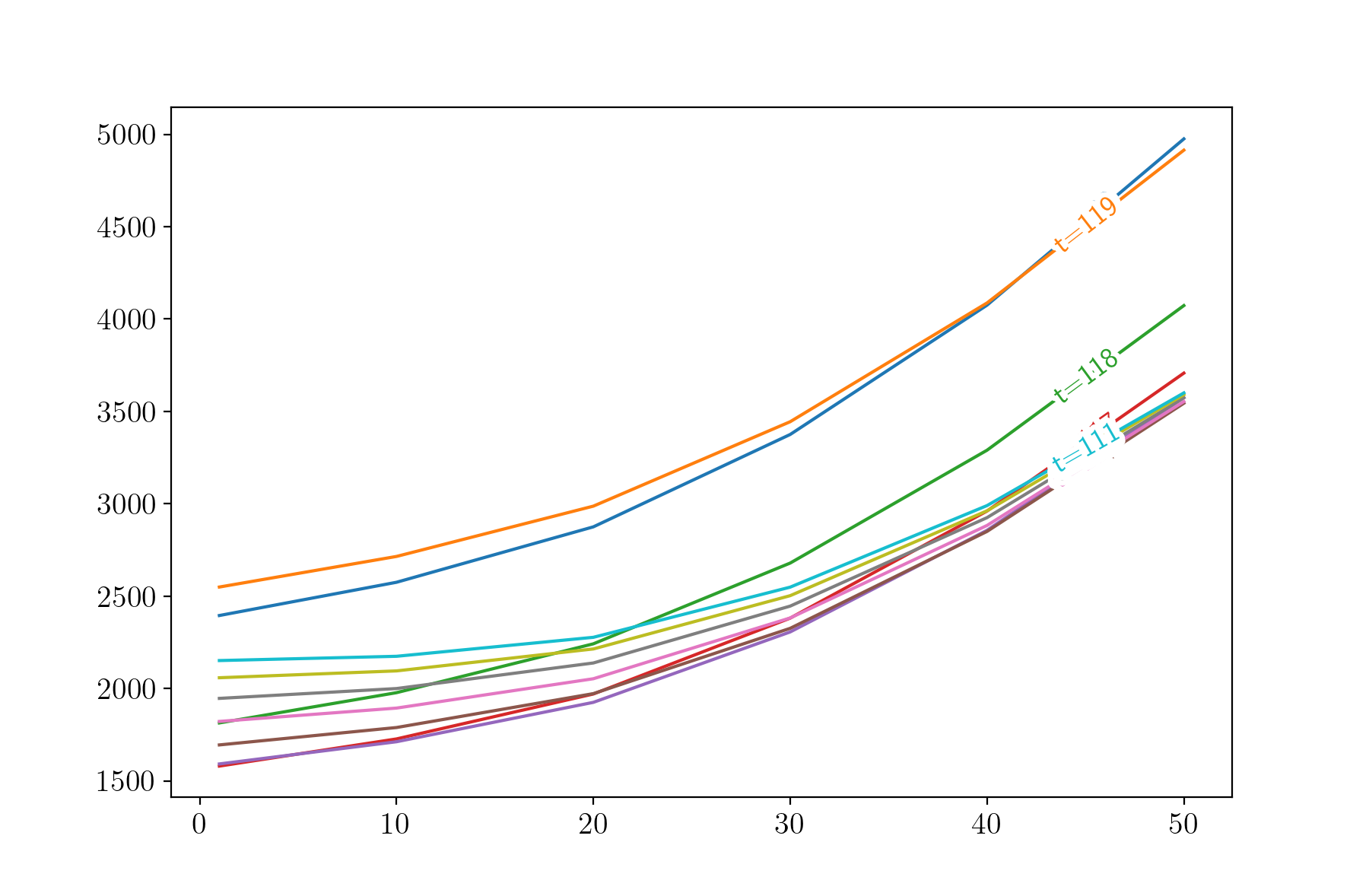
(f) Function of $z^{3}$, other variables moderate

Figure 18: Value function from linear interpolation approach (left) and regression approach
(right) as function of $z^{1}$, $m^{1}$ and $z^{3}$

Interpolation                 Regression

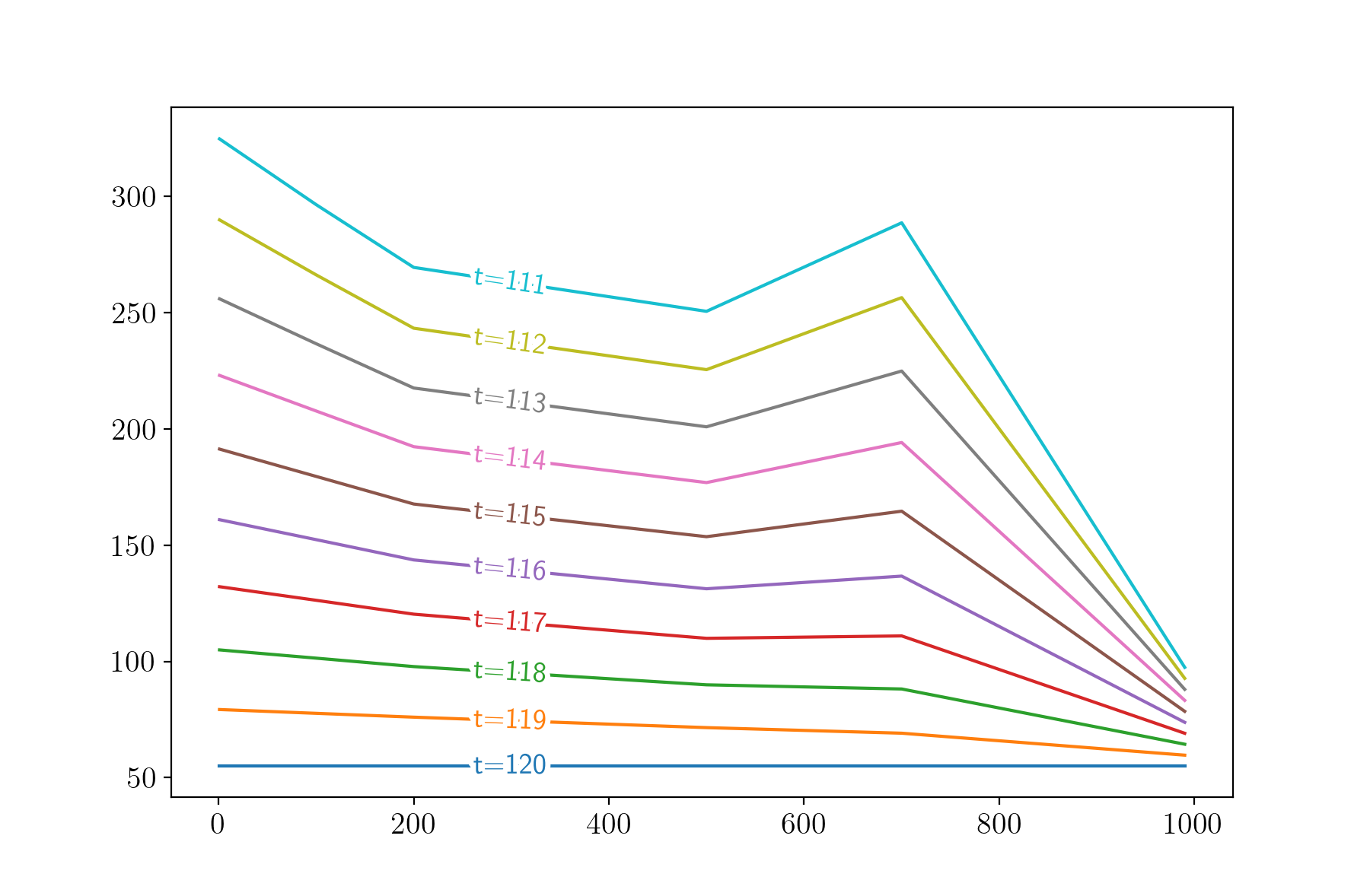
(a) Function of $z^{2}$, other variables small

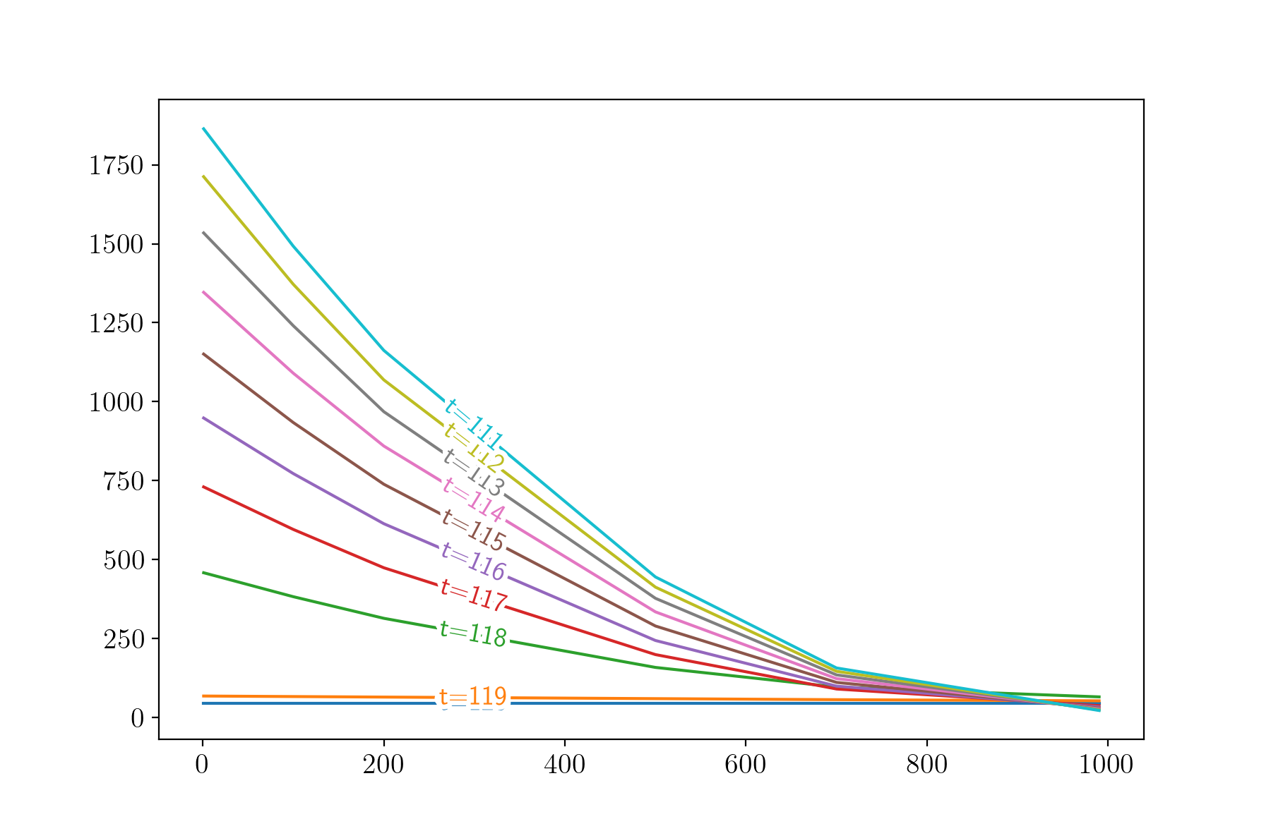
(b) Function of $z^{2}$, other variables small

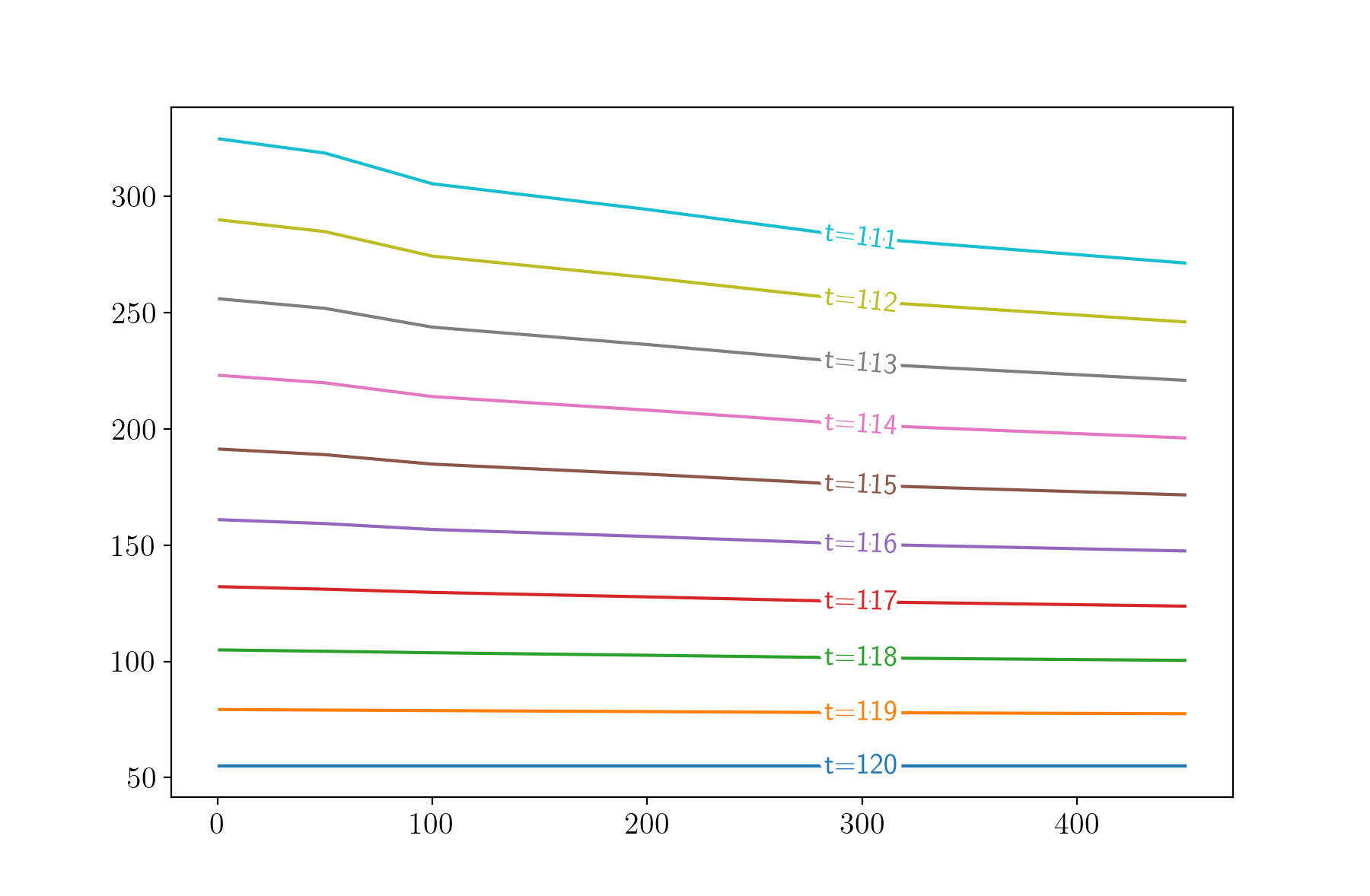
(c) Function of $m^{2}$, other variables small

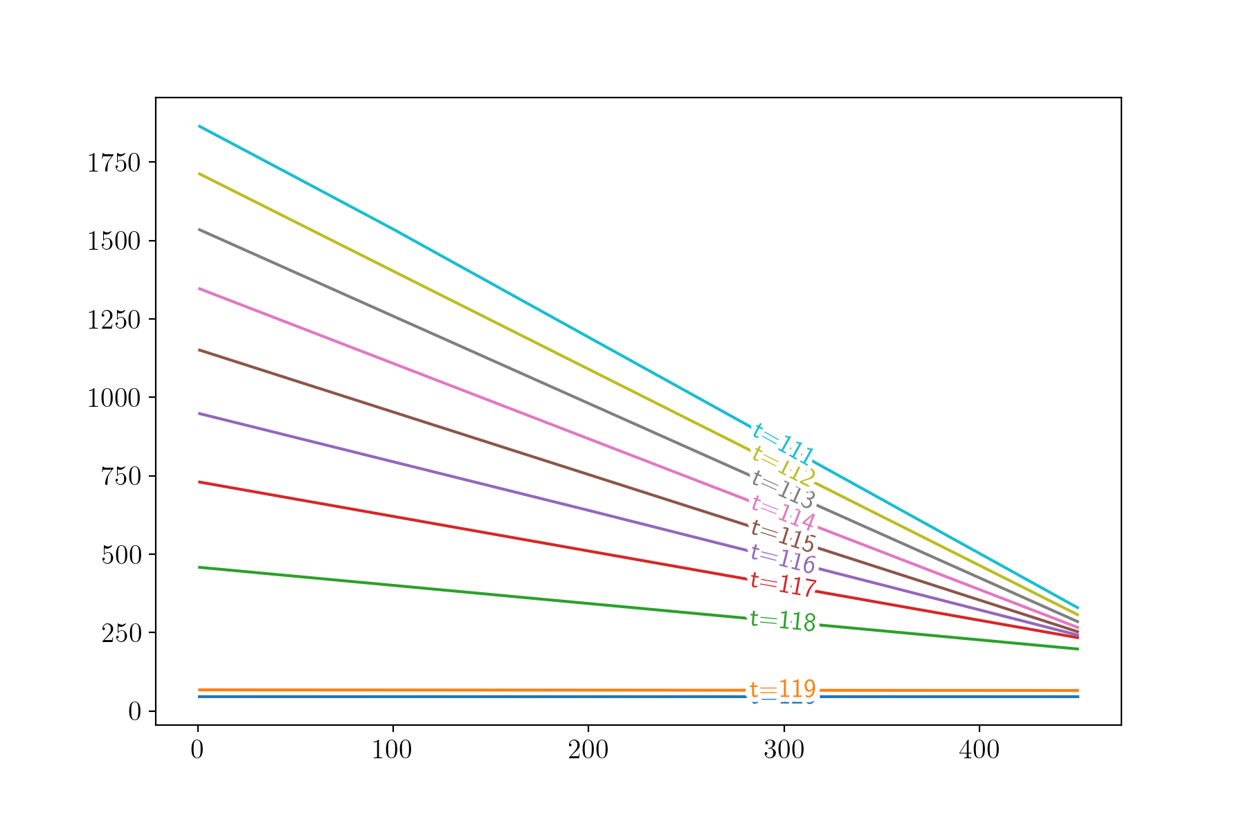
(d) Function of $m^{2}$, other variables small

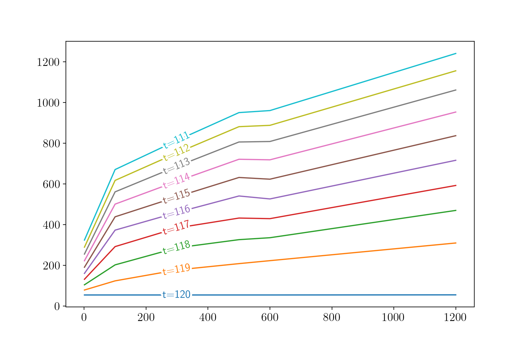
(e) Function of $q^{1}$, other variables small

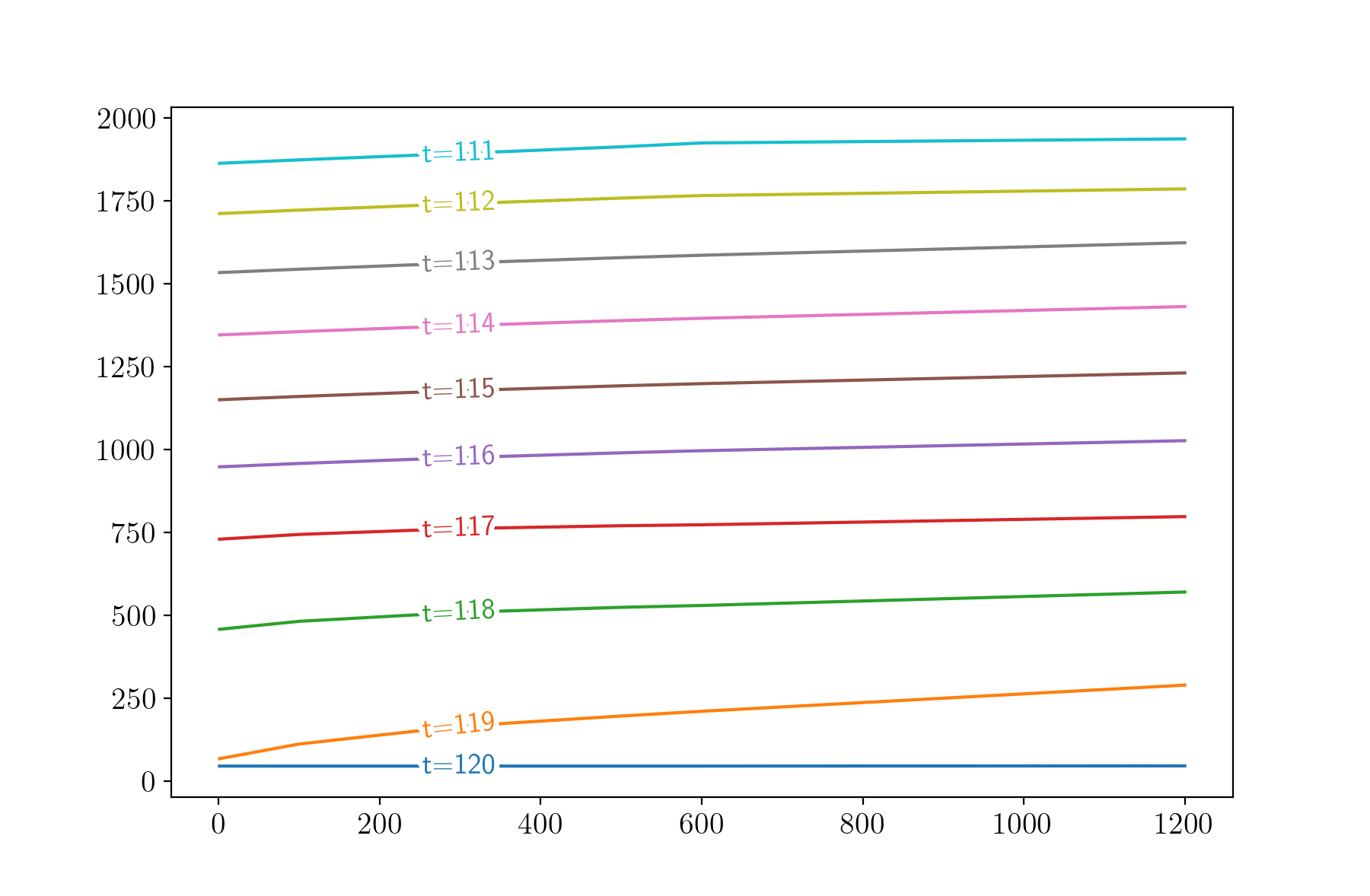
(f) Function of $q^{1}$, other variables small

Figure 19: Value function from linear interpolation approach (left) and regression approach (right) as function of $z^{2}$,$m^{2}$ and $q^{1}$

Interpolation                 Regression

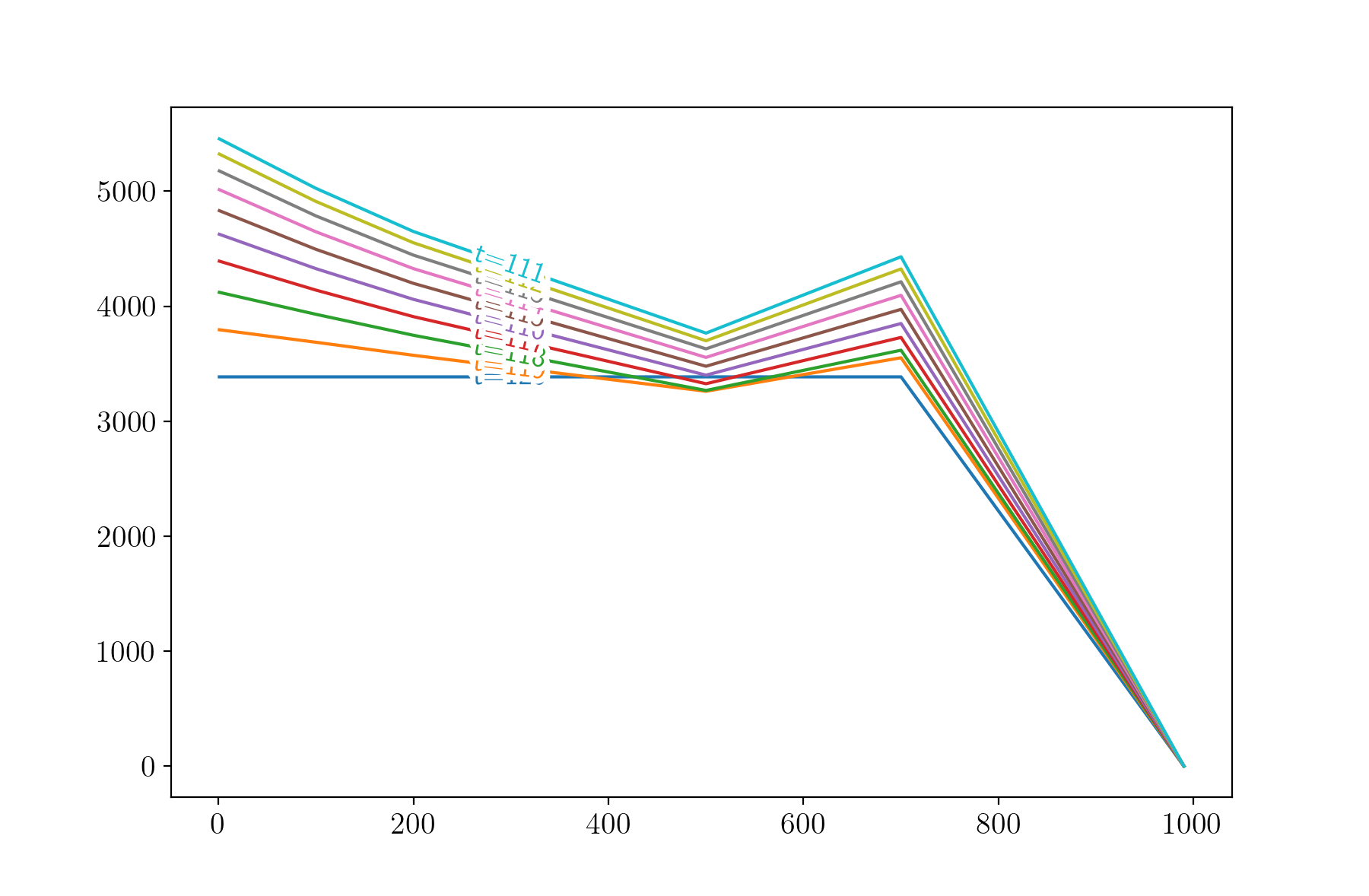
(a) Function of $z^{2}$, other variables moderate

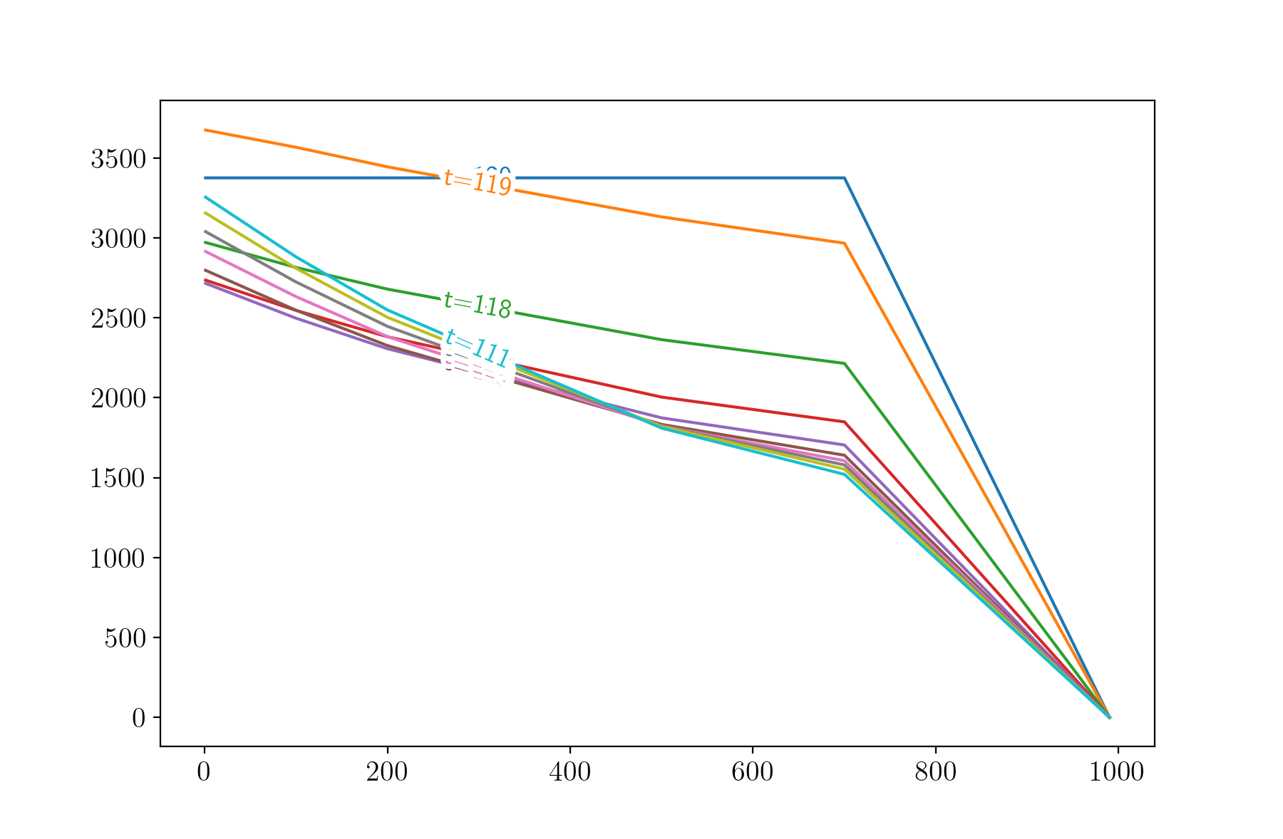
(b) Function of $z^{2}$, other variables moderate

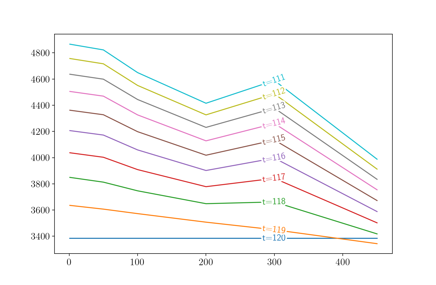
(c) Function of $m^{2}$, other variables moderate

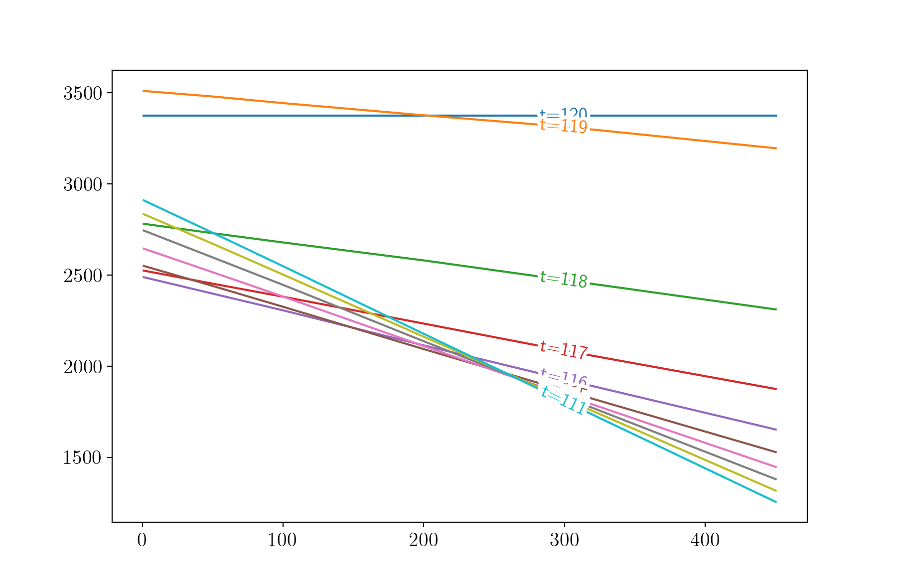
(d) Function of $m^{2}$, other variables moderate

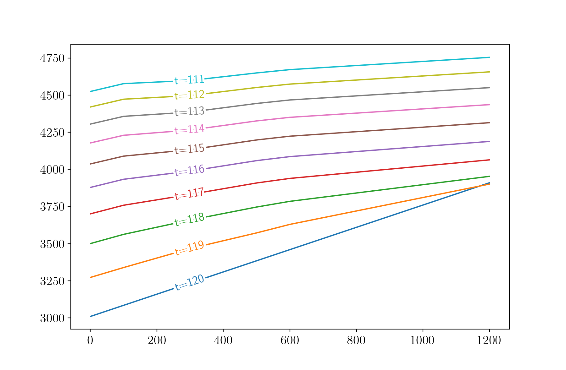
(e) Function of $q^{1}$, other variables moderate

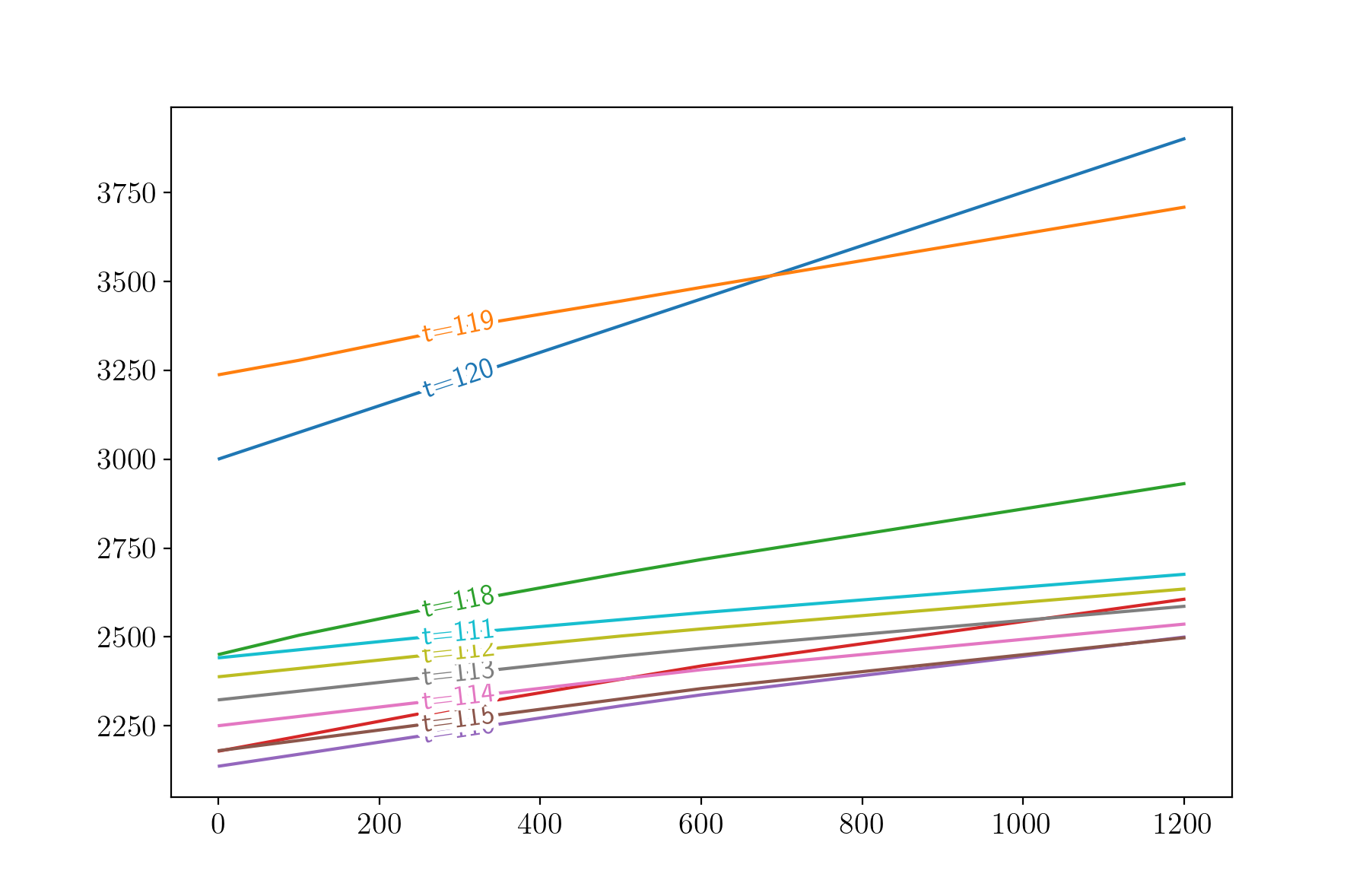
(f) Function of $q^{1}$, other variables moderate

Figure 20: Value function from linear interpolation approach (left) and regression approach (right) as function of $z^{2}$,$m^{2}$ and $q^{1}$

C.2 Value function obtained with regression method w.r.t. each component of the state

The behavior of the value function with respect to each compartment can also be visualized using the second method, regression. Figure 17( Panels 17(b),17(d),17(f)), Figure 18 ( Panels 18(b),18(d),18(f)), Figure 19( Panels 19(b),19(d),19(f)), and Figure20 ( Panels 20(b),20(d),20(f)) illustrate how the value functions vary w.r.t. each compartment size, while the other compartments are fixed at small and moderate values, similar to the first method results. We observe that the overall shape of the value function for each compartment aligns with the basis of the ansatz functions. However, some structural changes in the value function over time can be noted. For instance, in Figures 19 (Panels 19(d) and 19(f)), the value functions increase as the time is running backward and when the other components are kept small. Conversely, they generally decrease when the other components are kept moderate 20 (Panels 20(d) and 20(f)). This behavior differs from the results obtained with linear interpolation.

Appendix D List of Abbreviations

SIR, SIRS	Susceptible Infected Recovered with/without lifelong immunity)
$SI^{\pm}R^{\pm}H$	Suceptible Infected detected/non-detected Recovered detected/non-detected Hospitalized
Covid-19	Coronavirus disease 2019
ODE,SDE	Ordinary/Stochastic Differential Equation
SOCP	Stochastic optimal control problem
MDP	Markov decision process
CTMC	Continuous time Markov chain
EKF	Extended Kalman filter
NPI	Non-Pharmaceutical Intervention
ICU	Intensive Care Unit
HJB	Hamilton Jacobi Bellman
DPE	Dynamic programming equation
CLVQ	Competitive learning vector quantization
RBF	Radial basis functions

Appendix E List of Notations

H	hospitalized compartment
I, $I^{-}$, $I^{+}$	infected compartment, non-detected infected, detected infected compartment,
$R$, $R^{-}$, $R^{+}$	Recovered, non-detected, detected recovered
$S$	Susceptible compartment
$\rho$	correlation coefficient
$I^{+}_{max}$	upper bound of number of detected infected
$H_{max}$	upper bound of number of hospitalized
$M^{1}_{max},~M^{2}_{max}$	upper bound of $M^{1},~M^{2}$
$Q^{1}_{max},~Q^{2}_{max}$	upper bound of first and second diagonal entries $Q^{1},~Q^{2}$
$Q^{12}$	non-diagonal entry of the covariance matrix
$\pazocal{M}^{1},~\pazocal{M}^{2}$	set of discretized values of $M^{1},~M^{2}$
$\pazocal{Q}^{1},~\pazocal{Q}^{2}$	set of discretized values of $Q^{1},~Q^{2}$
$\pazocal{R}$	set of discretized values of $\rho$
$\pazocal{Z}^{1},\pazocal{Z}^{2},\pazocal{Z}^{3}$	sets of discretized values of $Z^{1},Z^{2},Z^{3}$
$\widetilde{M}^{1}$, $\widetilde{M}^{2}$	discretization values of $M^{1}$, $M^{2}$
$\widetilde{Q}^{1}$, $\widetilde{Q}^{2}$	discretization values of $Q^{1}$, $Q^{2}$
$\widetilde{Z}^{1}$, $\widetilde{Z}^{2}$, $\widetilde{Z}^{3}$	discretization values of $Z^{1}$, $Z^{2}$, $Z^{3}$
$x_{\widetilde{m}}$	generic grid point
$u^{L}$	social distancing or lockdown rate
$u^{T}$	Testing rate
$u^{V}$	vaccination rate
$u$	generic control sequence
$u^{T}_{min}$, $u^{T}_{max}$	minimum and maximum testing rate
$u^{V}_{max}$	maximum vaccination rate
$\pazocal{A}$	set of admissible control
$\pazocal{U}$	set of feasible control values
$u^{*}$	optimal control
$\widetilde{u}^{*}$	optimal decision rule
$\pazocal{U}^{D}$	set of discretized feasible control values
$\beta$	infection rate
$\alpha$	detection rate
$\eta^{-}$, $\eta^{+}$	hospitalization rate for non-detected, detected infected
$\gamma^{-}$, $\gamma^{+}$, $\gamma^{H}$	recovery rate for non-detected, detected, hospitalized infected
$M_{n}$	conditional mean at time $n\times\Delta t$
$Q_{n}$	conditional covariance at time $n\times\Delta t$
$n$	discrete time index
$N$	total population size
$N_{t}$	time index for terminal time $T=N_{t}\times\Delta t$
$X^{P}$	state process under partial information
$\pazocal{F}^{Z}_{n}$	observable $\sigma$-algebra at time $n$
$\pazocal{B}_{n}$	Gaussian sequence
$\pazocal{E}_{n}$	innovation sequence
$\overline{f}$	drift coefficient of the hidden state in continuous time
$\overline{\sigma}$, $\overline{g}$	first and second diffusion coefficient of the hidden state in continuous time
$\overline{h}_{0}$ $\overline{h}_{1}$	terms of drift coefficient of the observation in continuous time
$\overline{\ell}$	diffusion coefficient of the observation in continuous time
$f$	drift coefficient of the hidden state in discrete time
$\sigma$, $g$	first and second diffusion coefficient of the hidden state in discrete time
$h_{0}$ $h_{1}$	terms of drift coefficient of the observation in discrete time
$\ell$	diffusion coefficient of the observation in discrete time
$[A]^{+}$	pseudoinverse of the matrix $A$
$\pazocal{F}_{0}^{I}$	initial information $\sigma$-algebra
$\mathbb{I}$	identity matrix
$m_{0}$,$q_{0}$	initial values of conditional mean and conditional covariance
$C_{k}$	generic running cost function
$\overline{a}_{k}$, $a_{k}$, $b_{k}$	generic running cost coefficient
$a_{I^{-},N_{t}}$, $a_{I^{+},N_{t}}$, $b_{I^{-},N_{t}}$, $b_{I^{+},N_{t}}$	coefficient hidden, detected infection cost at terminal time
$\overline{x}$	threshold of the number of affected people
$C_{L}$, $C_{T}$, $C_{V}$, $C_{H}$	running lockdown, test, vaccination, hospitalization costs
$C^{\pm}_{I}$	running infection costs (detected/non-detected)
$X^{\text{work}}$	labor force within the population
$\overline{\text{x}}^{I^{\pm}}$	threshold for the number of infected (detected/non-detected)
$X^{\text{Test}}$	number of people who ca be tested
$\overline{\text{x}}^{\text{Test}}$	maximum capacity for testing
$\overline{\text{x}}^{\text{Vacc}}$	maximum capacity for vaccination
$\overline{\text{x}}^{\text{H}}$	maximum hospital capacity
$\Psi^{F}$, $\Phi^{F}$	running and terminal cost under full information
$\pazocal{J}^{F}$	expected aggregated cost under full information
$\mathbb{F}$	observable filtration
$\pazocal{J}$	expected aggregated cost under partial information
$\Psi$, $\Phi$	running and terminal cost under partial information
$f_{M},~g_{M}$	drift and noise coefficients of the conditional mean
$f_{Z},~g_{Z}$	drift and noise coefficients of the observation
$\pazocal{T}$	transition operator for $X^{P}$
$\pazocal{T}^{M}$, $\pazocal{T}^{Q}$, $\pazocal{T}^{Z}$	transition operator for conditional mean, conditional covariance, and observation
$\Phi_{\pazocal{N}}$	CDF of normal distribution
$\Gamma$	set of quantization points
$N_{l}$	number of quantization points or quantization level
$\xi_{l}$, $w_{l}$	quantization points and weights
$\varphi_{j}$	ansatz functions
$\theta_{j}$	ansatz functions regression coefficients
$\pazocal{I}$	set of grid points indexes
$\nu$	generic value of control
$W=(W^{1},W^{2})^{\top}$	$K$-dimensional standard Brownian motions

References

- Acemoglu et al. (2021) Acemoglu, D., Chernozhukov, V., Werning, I., Whinston, M.D., 2021. Optimal targeted lockdowns in a multigroup SIR-model. American Economic Review: Insights 3, 487–502.
- Al-Tawfiq (2020) Al-Tawfiq, J.A., 2020. Asymptomatic coronavirus infection: MERS-CoV and SARS-CoV-2 (Covid-19). Travel medicine and infectious disease 35, 101608.
- Alvarez et al. (2020) Alvarez, F., Argente, D., Lippi, F., 2020. A simple planning problem for Covid-19 lockdown. Covid Economics , 1.
- Anderson and Kurtz (2011) Anderson, D.F., Kurtz, T.G., 2011. Continuous time Markov chain models for chemical reaction networks, in: Design and analysis of biomolecular circuits: engineering approaches to systems and synthetic biology. Springer, pp. 3–42.
- Avram et al. (2022) Avram, F., Freddi, L., Goreac, D., 2022. Optimal control of a SIR epidemic with ICU constraints and target objectives. Applied Mathematics and Computation 418, 126816.
- Bäuerle and Rieder (2011) Bäuerle, N., Rieder, U., 2011. Markov decision processes with applications to finance. Springer Science & Business Media.
- Behncke (2000) Behncke, H., 2000. Optimal control of deterministic epidemics. Optimal control applications and methods 21, 269–285.
- Britton et al. (2019) Britton, T., Pardoux, E., Ball, F., Laredo, C., Sirl, D., Tran, V.C., 2019. Stochastic epidemic models with inference. volume 132. Springer.
- Calvia et al. (2024) Calvia, A., Gozzi, F., Lippi, F., Zanco, G., 2024. A simple planning problem for Covid-19 lockdown: a dynamic programming approach. Economic Theory 77, 169–196.
- Charpentier et al. (2020) Charpentier, A., Elie, R., Laurière, M., Tran, V.C., 2020. Covid-19 pandemic control: balancing detection policy and lockdown intervention under ICU sustainability. Mathematical Modelling of Natural Phenomena 15, 57.
- Day (2020) Day, M., 2020. Covid-19: identifying and isolating asymptomatic people helped eliminate virus in Italian village. BMJ: British Medical Journal (Online) 368, m1165.
- Federico and Ferrari (2021) Federico, S., Ferrari, G., 2021. Taming the spread of an epidemic by lockdown policies. Journal of mathematical economics 93, 102453.
- Federico et al. (2024) Federico, S., Ferrari, G., Torrente, M.L., 2024. Optimal vaccination in a SIRS epidemic model. Economic Theory 77, 49–74.
- Ferguson et al. (2020) Ferguson, N.M., Laydon, D., Nedjati-Gilani, G., Imai, N., Ainslie, K., Baguelin, M., Bhatia, S., Boonyasiri, A., Cucunubá, Z., Cuomo-Dannenburg, G., et al., 2020. Report 9: Impact of non-pharmaceutical interventions (NPIs) to reduce Covid-19 mortality and healthcare demand. volume 16. Imperial College London London.
- Garriga et al. (2022) Garriga, C., Manuelli, R., Sanghi, S., 2022. Optimal management of an epidemic: Lockdown, vaccine and value of life. Journal of Economic Dynamics and Control 140, 104351.
- Graf and Luschgy (2007) Graf, S., Luschgy, H., 2007. Foundations of quantization for probability distributions. Springer.
- Graf et al. (2007) Graf, S., Luschgy, H., Pagès, G., 2007. Optimal quantizers for Radon random vectors in a Banach space. Journal of Approximation Theory 144, 27–53.
- Guy et al. (2015) Guy, R., Larédo, C., Vergu, E., 2015. Approximation of epidemic models by diffusion processes and their statistical inference. Journal of Mathematical Biology 70, 621–646.
- Hansen and Day (2011) Hansen, E., Day, T., 2011. Optimal control of epidemics with limited resources. Journal of mathematical biology 62, 423–451.
- Hellewell et al. (2020) Hellewell, J., Abbott, S., Gimma, A., Bosse, N.I., Jarvis, C.I., Russell, T.W., Munday, J.D., Kucharski, A.J., Edmunds, W.J., Sun, F., et al., 2020. Feasibility of controlling Covid-19 outbreaks by isolation of cases and contacts. The Lancet Global Health 8, e488–e496.
- Hethcote and Waltman (1973) Hethcote, H.W., Waltman, P., 1973. Optimal vaccination schedules in a deterministic epidemic model. Mathematical Biosciences 18, 365–381.
- Hu and Zou (2013) Hu, Q., Zou, X., 2013. Optimal vaccination strategies for an influenza epidemic model. Journal of Biological Systems 21, 1340006.
- Ishikawa (2012) Ishikawa, M., 2012. Stochastic optimal control of an SIR epidemic model with vaccination, in: Proceedings of the ISCIE International Symposium on Stochastic Systems Theory and its Applications, The ISCIE Symposium on Stochastic Systems Theory and Its Applications. pp. 57–62.
- Jakobsson et al. (2009) Jakobsson, S., Andersson, B., Edelvik, F., 2009. Rational radial basis function interpolation with applications to antenna design. Journal of computational and applied mathematics 233, 889–904.
- Kantner and Koprucki (2020) Kantner, M., Koprucki, T., 2020. Beyond just “flattening the curve”: Optimal control of epidemics with purely non-pharmaceutical interventions. Journal of Mathematics in Industry 10, 23.
- Kermack and McKendrick (1927) Kermack, W.O., McKendrick, A.G., 1927. A contribution to the mathematical theory of epidemics. Proceedings of the royal society of london. Series A, Containing papers of a mathematical and physical character 115, 700–721.
- Kruse and Strack (2020) Kruse, T., Strack, P., 2020. Optimal control of an epidemic through social distancing. Available at SSRN 3581295 .
- Laguzet and Turinici (2015) Laguzet, L., Turinici, G., 2015. Global optimal vaccination in the SIR model: properties of the value function and application to cost-effectiveness analysis. Mathematical biosciences 263, 180–197.
- Landsgesell and Stadler (2020) Landsgesell, L., Stadler, M., 2020. The spread of Covid-19 in Germany: An application of the SIRDH model. Technical Report. University of Tübingen Working Papers in Business and Economics.
- Larédo and Tran (2020) Larédo, C., Tran, V.C., 2020. Statistical inference for epidemic processes in a homogeneous community. In: Stochastic Epidemic Models and Inference, ed. T. Britton, E. Pardoux,325-472 .
- Ledzewicz and Schättler (2011) Ledzewicz, U., Schättler, H., 2011. On optimal singular controls for a general SIR-model with vaccination and treatment, in: Conference Publications, Conference Publications. pp. 981–990.
- Liptser and Shiryaev (2013) Liptser, R.S., Shiryaev, A.N., 2013. Statistics of random processes II: Applications. volume 6. Springer Science & Business Media.
- Mbouandi Njiasse et al. (2025) Mbouandi Njiasse, I., Ouabo Kamkumo, F., Wunderlich, R., 2025. State estimation in stochastic epidemic models under partial information. Working paper .
- Miclo et al. (2022) Miclo, L., Spiro, D., Weibull, J., 2022. Optimal epidemic suppression under an ICU constraint: An analytical solution. Journal of Mathematical Economics 101, 102669.
- Nowzari et al. (2016) Nowzari, C., Preciado, V.M., Pappas, G.J., 2016. Analysis and control of epidemics: A survey of spreading processes on complex networks. IEEE Control Systems Magazine 36, 26–46.
- Ouabo Kamkumo et al. (2025) Ouabo Kamkumo, F., Mbouandi Njiasse, I., Wunderlich, R., 2025. Stochastic epidemic models with partial information. Submitted to arxiv.org .
- Pagès (1998) Pagès, G., 1998. A space quantization method for numerical integration. Journal of computational and applied mathematics 89, 1–38.
- Pagès (2018) Pagès, G., 2018. Numerical probability. Universitext, Springer .
- Pflug and Pichler (2011) Pflug, G.C., Pichler, A., 2011. Approximations for probability distributions and stochastic optimization problems. Stochastic optimization methods in finance and energy: New financial products and energy market strategies , 343–387.
- Regis (2014) Regis, R.G., 2014. Constrained optimization by radial basis function interpolation for high-dimensional expensive black-box problems with infeasible initial points. Engineering Optimization 46, 218–243.