Non-perturbative asymptotics of the eigenvalues of the spheroidal equation

Abstract

New non-perturbative results on the eigenvalues of the spheroidal equation are presented. The results, found using an all orders WKB analysis, include a perturbative/non-perturbative (P/NP) relation as well as the first exponential correction to the perturbative series which is valid in certain regions of parameters. The quantum periods are also computed.

1 Introduction

This article addresses the spectrum of the spheroidal equation

$$\left(-\frac{\hbar^{2}}{2}\derivative[2]{x}+\cos^{2}x+\mu\csc^{2}x-E\right)\psi(x)=0.$$ (1)

The new contributions presented here are a perturbative/non-perturbative (P/NP) relation, which shows that the non-perturbative terms of the transseries expansion for the eigenvalues of the spheroidal equation are entirely expressible in terms of perturbative quantities. Additionally, we provide systems of Picard-Fuchs differential operators which encode the quantum actions and thereby lay the foundations for analytic computations of the spectra of the spheroidal equation in multiple regions of parameter space and in various contexts.

We explicitly compute a low energy expansion of the eigenvalue as well as the first non-perturbative correction in the region $-1<\mu<0$ (see figure 1). The non-perturbative terms provided are then checked using a numerical resurgent analysis. Because of the dependence of the perturbative spectra on the level number and the parameter $\mu$ this analysis offers insight into parametric resurgence.

The spheroidal equation (1) reduces to the Mathieu equation when the parameter $\mu$ is set to zero. In addition, if the $\cos^{2}x$ term is removed from the potential the spheroidal equation is equivalent to the Legendre equation. The singularities of the potential $V(x)=\cos^{2}x+\mu\csc^{2}x$ at integer multiples of $\pi$ make the limit $\mu\to 0$ subtle. This is particularly true for the non-perturbative terms of the transseries and is addressed in section 4.2.

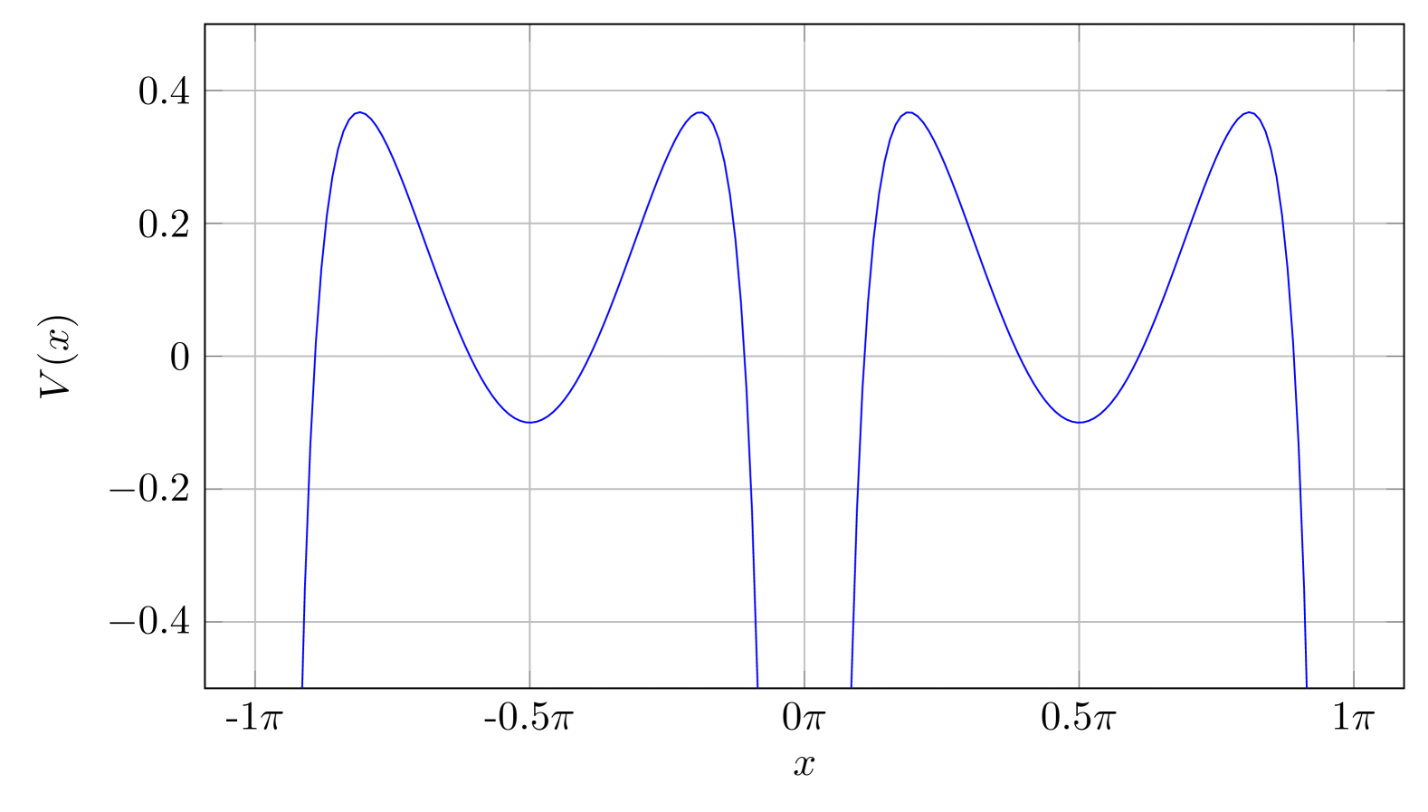
(a) The region $-1<\mu<0$.

(b) The region $\mu<-1$.

(c) The region $0<\mu$.

Figure 1: The spheroidal potential, $V(x)=\cos^{2}x+\mu\csc^{2}x$, plotted in the three distinct regions of the parameter $\mu$. This paper provides perturbative and non-perturbative expansions of the eigenvalue in the case $-1<\mu<0$.

1.1 Several threads in the literature

The significance of the spheroidal equation to both mathematics and to physics cannot be understated. While, the prolate/oblate spheroidal equations appear in classical mathematical physics—the study of a oscillations of a spheroid—the prolate spheroidal equation surprisingly appears in information/communication theory doi:10.1073/pnas.2207652119 ; Slepian . When the mathematical foundations of signal processing were being developed C. Shannon sought to refine the following well known statement coming from quantum mechanics: It is not possible to simultaneously concentrate a wave-function in position and momentum spaces. This led to the following question doi:10.1073/pnas.2207652119 : Suppose you have a band-limited signal—which you observe for some finite time interval. What is the best use you can make of your observations? This question was answered by Slepian, Landau, and Pollak in the 1960s Slepian ; 6773659 ; 6773660 . At the heart of their work is a certain integral equation—whose solution describes the signal which maximizes the concentration of a band limited signal in the time domain—which has the same eigenfunctions as the prolate spheroidal equation doi:10.1073/pnas.2207652119 ; Slepian .

The results of Slepian, Landau, and Pollak have since been generalized. For instance, Grünbaum Grunbaum_2021 has provided a family of integral operators with commuting differential equations. Further, Grünbaum established a connection between the master symmetries of the KdV hierarchy and this extension of Slepian’s result. Additionally, Longo Longo:2023ssd provided an interpretation of the prolate spheroidal operator as an entropy operator, adding clarification to the ‘lucky accident’ that the eigenfunctions of the integral equation found by Slepian, Pollak and Landau are prolate spheroidal functions.

A second remarkable appearance of the spheroidal equation was discovered by A. Connes connesTraceFormulaNoncommutative1999 . In connesTraceFormulaNoncommutative1999 A. Connes gave a spectral interpretation of the zeros of the Riemann zeta function. The appearance of the spheroidal equation as described in ConnesMarcolli is due to the delicate point that obtaining the counting of modes in the corresponding quantum system involves both an ultraviolet and infrared cutoff. However, because it is impossible to impose a cutoff of both a function and its Fourier transform, Connes utilized the result of Slepian—cutoffs can be approximated using the prolate spheroidal wavefunctions.

This has led to a line of research into the spheroidal equation including FauvetF.2010Spft ; JungRamisFauvetThomann ; doi:10.1073/pnas.2123174119 ; ConnesMarcolli ; connes2021spectraltripleszetacycles ; connes2024zetazerosprolatewave . For example, FauvetF.2010Spft sought to answer the challenge posed in Slepian of Slepian to find an abstract perspective on the spheroidal wave functions “that will explain their elegant [properties] in a more natural and profound way." The work of Richard-Jung et al FauvetF.2010Spft provided a fist step in this direction. With a perspective rooted in Riemann-Hilbert theory Richard-Jung et al found new results on the Stokes phenomenon of the spheroidal functions and interpreted them in terms of differential Galois theory. This was followed by JungRamisFauvetThomann where the same authors investigated the eigenvalues of the (prolate) spheroidal equation and provided a novel method for computing them numerically from the zeros of certain polynomials.

We remark that the results presented here are relevant to this line of research. As will be discussed in section 2, the exact WKB method is closely related to Riemann-Hilbert theory. Some further relevance is furnished by doi:10.1073/pnas.2123174119 , in which Connes and Moscovici identified new relationships between the spectrum of the prolate spheroidal operator and the zeros of Riemann zeta function in a semiclassical limit.

Another surprising appearance of the spheroidal equation—this time in physics—comes from bilayer graphene ChoiMin-Young2011Adot ; Hyun_2012 . In deGailGraphene a low energy effective hamiltonian describing the Landau level spectrum of quasiparticles in twisted bilayer graphene was proposed and motivated. The eigenvalues of the hamiltonian were shown to be expressed exactly in terms of spheroidal eigenvalues ChoiMin-Young2011Adot . Further theoretical grounding for the simplified model used in ChoiMin-Young2011Adot has been offered more recently beckerMagneticResponseProperties2024 .

As noted in ChoiMin-Young2011Adot the difference between adjacent Landau levels is controlled by non-perturbative structure in the expansion parameter. This non-perturbative behavior describes the asymptotic degeneracy found by the decoupling of the two layers of graphene as the twist angle increases. Within the model used by ChoiMin-Young2011Adot ; deGailGraphene the non-perturbative structure of the spheroidal eigenvalues encodes the transition between the massive and massless regions of the spectra. The relevance of the non-perturbative structure of the spheroidal eigenvalues to graphene provides good motivation for a systematic investigation of the non-perturbative properties of the eigenvalues as well as an investigation into various physical contexts in which they may have influence.

Some non-perturbative features of the spheroidal equation have been investigated previously by Müller-Kirsten in Muller+1963+26+48 . The perturbative and non-perturbative expansions which we compute were chosen to match those computed by Müller-Kirsten. Besides notational differences the analysis provided here uses a slightly different expansion parameter. We recover Müller-Kirsten’s expansions in the limit $\mu\propto\hbar$, and in this sense our results carry additional nonperturbative information.

A substantial amount of interest in the spheroidal equation is due to the fact that the spheroidal equation plays a fundamental role in the physics of rotating black holes TeukolskyThesis . In 1973, Teukolsky TeukolskyThesis separated the equation describing perturbations of the Kerr metric. The resulting separated equation is known as the Teukolsky equation. It describes both perturbations of the Kerr geometry as well as scalar, vector and tensor fields in a Kerr background. The Teukolsky equation consists of two parts, a radial equation, and an angular equation. Together, with proper boundary conditions, they encode the quasinormal mode frequencies of black hole radiation. The angular equation takes the form of the spin weighted spheroidal equation. By setting the ‘spin’ to zero, the equation reduces to the spheroidal equation.

Quasinormal modes of black holes are particularly well studied due to the explosion of interest created by the LIGO gravitational wave observations. That being said, analytic methods have been limited to a small number of techniques. In particular, two of the most commonly applied are Leaver’s continued fraction method doi:10.1098/rspa.1985.0119 ; Berti_2009 and the WKB method PhysRevD.35.3621 ; Seidel:1989bp ; Yang_2013_Branching ; Konoplya:2003ii ; Konoplya:2019hlu ; Konoplya:2023moy ; Matyjasek_2017 .

Leaver’s continued fraction method doi:10.1098/rspa.1985.0119 was first applied to the perturbations of the Schwarzschild metric but was adapted to Kerr black holes as well as other geometries. Notably, it was applied by Berti, Cardoso and Starinets in Berti_2009 for a number of quasinormal mode calculations. It functions using a series ansatz to both radial and angular equations which take into account the appropriate boundary conditions. The WKB method has been applied extensively PhysRevD.86.104006 ; Seidel:1989bp ; PhysRevD.35.3621 ; PhysRevD.35.3632 ; PhysRevD.37.3378 , often including higher order terms in the expansion. Some examples are Seidel:1989bp ; Konoplya_2003 ; Konoplya:2019hlu ; Matyjasek_2017 which go beyond leading order. An interesting comparison is to the work of Imaizumi in Imaizumi::2022 ; Imaizumi::2023 , who applied the exact WKB method to the computation of quasinormal modes of D3 and M5 branes. A notable difference comes from Imaizumi’s use of summation techniques such as Borel-Padé summation which have been shown (see for instance Costin:2020hwg ) to improve upon the standard Padé approximant techniques such as those used in Konoplya_2003 ; Konoplya:2019hlu ; Seidel:1989bp ; Matyjasek_2017 .

Imaizumi’s analysis fits into a larger context—a recent influx of results on quasinormal modes supplied by the particle physics community fioravanti2022integrabilitysusysu2matter ; fioravanti2022newmethodexactresults ; Aminov2020 ; Bonelli:2021uvf ; bianchiMoreSWQNMCorrespondence2022 ; Aminov:2023jve ; Arnaudo:2024rhv ; Arnaudo:2024bbd ; Hatsuda:2021gtn ; Hatsuda_2020 ; Hatsuda_2021 ; Silva:2025khf . The connection between these topics is in large part due to the fact that Teukolsky’s equation (and therefore the spheroidal equation) is a special case of a confluent Heun equation Borissov:2009bj ; Aminov2020 ; Bautista:2023sdf . A more detailed discussion of some of this research is provided in section 2.

1.2 Black hole dictionary

For reference, we provide a dictionary connecting the notation used here to the black hole parameters used in the study of quasinormal modes. The spheroidal equation in the black hole parameters is listed in Aminov2020 , when in Liouville normal form it is

$$\left(\derivative[2]{\theta}+\lambda_{lm}+\frac{1}{4}+\omega^{2}a^{2}\cos^{2}\theta+\left(\frac{1}{4}-m^{2}\right)\csc^{2}\theta\right)S_{m}^{l}(\theta)=0$$ (2)

where $a$ is the angular momentum per unit mass of the black hole and ranges between $0$ and $M$. The parameter $M$ is the mass of the black hole. The parameters $\lambda_{lm}$ are the separation constants. The labels $m,l$ are the azimuthal and angular harmonic indices. The quasi-normal mode frequency is given by $\omega$. The boundary conditions come from a regularity condition at the poles of $\csc\theta$ which can be found in Aminov2020 or TeukolskyThesis .

This equation is equivalent to equation (1). Specifically, the black hole spheroidal equation (2) is transformed into equation (1) under the identifications

$$\hbar=\frac{i\sqrt{2}}{a\omega}, E=-\frac{1}{a^{2}\omega^{2}}\left(\lambda^{l}_{m}+\frac{1}{4}\right), \mu=\frac{1}{a^{2}\omega^{2}}\left(\frac{1}{4}-m^{2}\right).$$ (3)

Let $0<\zeta\leq 1$. Because the angular momentum per black hole mass must satisfy $0\leq a\leq M$ the limit $\hbar\to 0$ corresponds to the double limit $a\to\zeta M$ and $M\to\infty$. This describes a large black hole which is spinning with angular momentum per unit mass $a$ of order of the mass. This is not the same as the extremal limit.

2 The exact WKB method

The WKB method can be extended beyond leading order to provide formal series solutions to eigenvalue problems Dunham_1932 . These formal asymptotic series are divergent but can be resummed and their monodromy and Stokes phenomenon understood using the framework of exact WKB Voros::1983 ; Delabaere1997ExactSE ; Bucciotti:2023trp ; vanSpaendonck:2023znn . In particular, eigenvalues of differential operators can be computed analytically from exact quantization conditions. The building blocks of these conditions are ‘Voros symbols’ or quantum actions. In section 2.1 we review the standard definition of the quantum actions as well as the Bohr-Sommerfeld condition which allows for calculation of perturbative expansions of eigenvalues. In section 3 we conjecture a form for the first non-perturbative, exponential correction to the perturbative expansion for the energy level. In section 4.3 we provide a numerical resurgent analysis verifying the proposed non-perturbative asymptotics and computing the Stokes constant.

For the spheroidal equation the exact WKB method is closely related to $SU(n)$, $\mathcal{N}=2$ supersymmetric gauge theory Grassi_2022 ; Aminov2020 ; Yan:2020kkb . More specifically, some Schrödinger equations (including the Heun equation and therefore the spheroidal equation) are described by $\mathcal{N}=2$ supersymmetric gauge theories placed in the Nekrasov-Shatashvili limit of the $\Omega$-background. In this connection, the classical equation of motion corresponding to the Schrödinger operator appears as the Seiberg-Witten curve of the field theory with $\hbar$ playing the role of the $\Omega$-background parameter ‘$\epsilon_{1}$.’ The classical period integrals, describing the action of a periodic trajectory, control the masses and central charges of BPS states, while the full series of quantum actions can be computed in terms of the Nekrasov-Shatashvili instanton counting function Grassi_2022 . In fact, in Aminov2020 Aminov, Hatsuda and Grassi used this connection to relate the quasinormal modes of rotating black holes, (and therefore the eigenvalues of the spheroidal equation), to the Nekrasov-Shatashvili instanton counting function. More details on the connection between exact WKB and $\mathcal{N}=2$ supersymmetric field theories is available in comanQuantumCurvesTopological2025 .

WKB periods can also be calculated with thermodynamic-Bethe-ansatz (TBA) equations Imaizumi::2020 ; Imaizumi::2021 ; Emery_2021 ; Ito_2019 ; Ito2023 . The TBA approach is perhaps the most efficient approach for calculating quantum periods and solving exact quantization conditions numerically. The TBA approach however does not produce asymptotic series with full parameter dependencies included. As described in Ito_2019 , the seminal work of Voros Voros::1983 provided a method for computing spectral data from exact quantization conditions using what was termed the “analytic bootstrap.” In this approach the WKB periods play a fundamental role and are Borel resummed to form exact quantization conditions. The discontinuity structure encoded by the Stokes automorphism of the WKB periods determines a Riemann-Hilbert problem which has a solution in terms of a TBA-like system Ito_2019 . The connection between TBA and differential equations, the ODE/IM correspondence Dorey_1999 , has been used for the calculation of quasinormal modes fioravanti2022newmethodexactresults of D3 branes and the Reissner-Nordström geometry. However, to the knowledge of the author it has not been applied to the case of Kerr black holes.

As a final comment we mention that exact quantization conditions can also be solved analytically in terms of transseries vanSpaendonck:2023znn . Here we lay the foundation for such computations. For this reason we focus on the computation of the quantum actions exactly and with full parameter dependence included.

2.1 Quantum actions and the Bohr-Sommerfeld condition

Applying a WKB ansatz $\psi(x)=e^{\frac{i}{\hbar}\int^{x}\phi\differential{x}}$ to the Schrödinger equation (1) gives the following Riccati equation

$$\phi^{2}=2(E-\cos^{2}x-\mu\csc^{2}x)-i\hbar\derivative{x}\phi.$$ (4)

Setting $\hbar=0$, this equation is algebraic and coincides with the classical equation of motion with the action density $\phi$ playing the role of momentum. In the complex domain the classical equation of motion defines a Riemann surface which happens to be a torus, call it $\Sigma$.

The equation (4) has an asymptotic series solution Dunham_1932 for the action density $\phi$. Let

$$\phi(\mu,E,\hbar,x)=\sum_{k=0}^{\infty}\phi_{k}(\mu,E,x)\hbar^{k}.$$ (5)

Each of the $\phi_{k}\differential{x}$ are differentials on the Riemann surface $\Sigma$. More precisely they are differentials on $\Sigma$ where the points $x=\dots,-2\pi,-\pi,0,\pi,\dots$ (which correspond to simple poles of the $\phi_{k}$) are removed. This means that we can integrate them along paths on $\Sigma$ and define quantum actions.

The Quantum Actions.

Let $\gamma$ be a cycle on $\Sigma$ then the quantum action along $\gamma$ is defined to be

$$N_{\gamma}(E,\mu,\hbar)=\sum_{k=0}^{\infty}\left(\oint_{\gamma}\phi_{k}(\mu,E,x)\differential x\right)\hbar^{k}.$$ (6)

Because $\Sigma$ is a torus there are two independent cycles. Call them $A,B$ and choose $A$ so that it corresponds to a classical periodic orbit. One way to identify $A$ and $B$ is to construct $\Sigma$ using the ‘cut-and-paste’ method. In this perspective the $A$ cycle should be chosen to move around the classical turning points associated to a well of the potential. These turning points coincide with ramification points of $\Sigma$ which the ‘cuts’ must connect.

The Bohr-Sommerfeld Condition.

Let $l\in\mathbb{N}_{0}$. The solution $E_{A}(l,\mu,\hbar)$ to the following equation

$$2\pi\hbar l=N_{A}(E_{A},\mu,\hbar)$$ (7)

is an asymptotic expansion for the $l$th eigenvalue of the Schrödinger equation in the limit $\hbar\to 0$ and $l\to\infty$ such that the limit of the product $\hbar l$ is fixed and proportional to the classical action. The limit is analogous to a t’Hooft double scaling limit LoChiatto:2023bam .

The low energy expansion of the quantum actions can be used to generate all orders of the Rayleigh-Schrödinger perturbative series associated to $A$. In particular, the perturbative series for the energy is determined by calculating the ‘low energy’ expansion of the quantum action $N_{A}(E,\mu,\hbar)$ and then by solving the Bohr-Sommerfeld condition for $E_{A}$ using series inversion. After calculating the quantum action to in section 2.4 we use this approach to find the perturbative series for $E_{A}(l,\mu,\hbar)$ in section 2.5.

2.2 The classical actions

At the classical level the actions are given by integrals of the form

$$N_{0,\gamma}(E,\mu)=\int_{\gamma}\sqrt{2(E-\cos^{2}x-\mu\csc^{2}x)}\differential x$$ (8)

where $\gamma$ is a cycle on the Riemann surface $\Sigma$. For each $\gamma$ the classical actions can be expressed in terms of elliptic integrals of the first, second and third kinds. The elliptic integrals are denoted by $\mathbf{K},\mathbf{E},\mathbf{\Pi}$ the complete elliptic integrals of the first, second and third kinds, respectively. To fix notation they are defined in appendix A. In order to define the classical action and dual action let

$$k_{\pm}=\sqrt{\frac{E\mp\sqrt{(E-1)^{2}+4\mu}+1}{E\pm\sqrt{(E-1)^{2}+4\mu}+1}} \nu_{\pm}=\frac{\mp\sqrt{(E-1)^{2}+4\mu}+E-1}{\mp\sqrt{(E-1)^{2}+4\mu}+E-1-2\mu}.$$ and, (9)

In addition, let

$$G(\nu,k)=\frac{\sqrt{2}}{\nu^{3/2}}\Bigg{(}\left(\nu-1\right)\left(k^{2}-\nu\right)\mathbf{\Pi}\!\left(\nu,k\right)+\nu\,\mathbf{E}\!\left(k\right)+\left(k^{2}-\nu\right)\mathbf{K}\!\left(k\right)\Bigg{)}.$$ (10)

The definition of the $A$ and $B$ cycles depends on the value of the parameters $\mu$ and $E$, as these determine both the shape of the potential as well as the classical and non-classical regions. Here we focus on the region of parameters $-1<\mu<0$. In this case the harmonic well defining the $A$ cycle is separated from an infinitely deep well associated to a pole of the potential by two finite barriers on either side, see figure 2. On one hand, it might be expected that the $B$ cycle describes the tunneling rate out of the harmonic well and into the infinitely deep well. On the other, the $B$ cycle could be determined by a trajectory which tunnels between neighboring harmonic wells. The difference between the choices is an overall factor of two as well as a contribution coming from the residue of the pole.

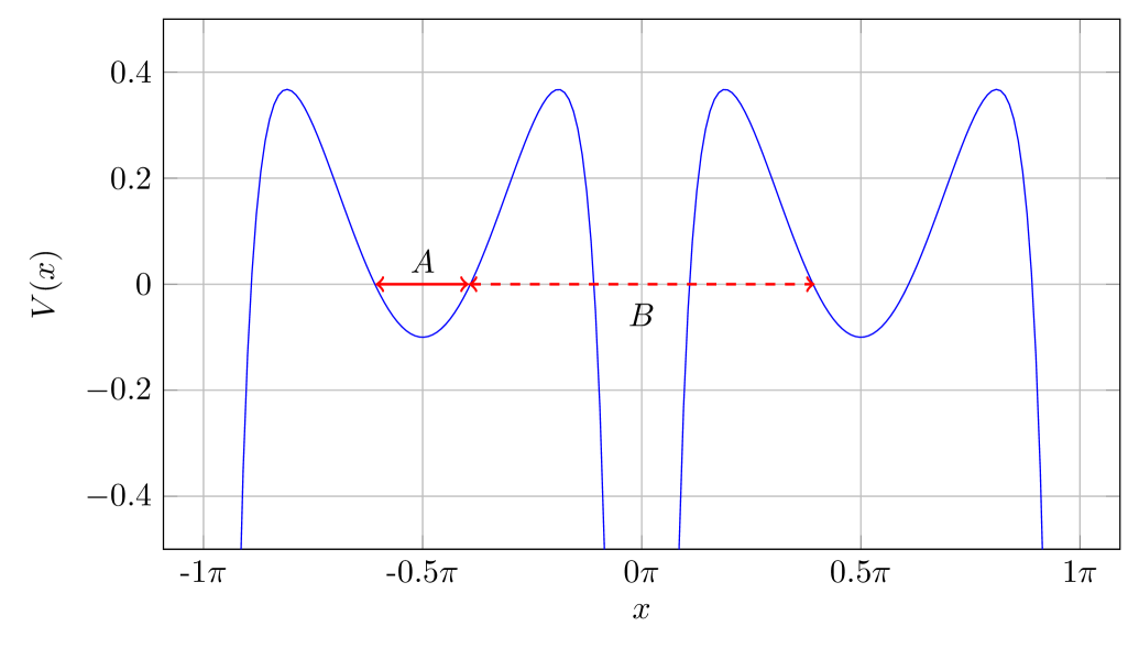
Figure 2: The figure shows the potential in the region $-1<\mu<0$ with the $A$ and $B$ cycles sketched by the solid and dashed arrows respectively. The harmonic well defining the $A$ cycle is separated from an infinitely deep well associated to a pole by a finite barrier.

Numerical tests show that the second interpretation ‘tunneling between harmonic wells’ is responsible for the leading non-perturbative behavior. This has the interesting consequence that the leading non-perturbative structure of the spheroidal eigenvalue in this region reduces to that of the Mathieu equation in the limit $\mu\to 0$.

In this region and with the above cycles, the action, associated to the cycle $A$, and the dual action, associated to the cycle $B$, are given by

$$N_{0,A}(E,\mu)=G(\nu_{+},k_{+})-2\sqrt{2\mu} N_{0,B}(E,\mu)=G(\nu_{-},k_{-}).$$ and (11)

2.3 Picard-Fuchs differential operators

The WKB expansion is intimately tied to the geometry of the Riemann surface $\Sigma$. In particular, variations of the parameters $(\mu,E)$ lead to deformations of $\Sigma$. However, for each pair $(\mu,E)\in\mathbb{C}$ (away from critical points) the Riemann surfaces are diffeomorphic. The deformation is therefore not ‘topological,’ but occurs at the level of the underlying complex/Hodge structure.

Varying the parameters leads to the ‘monodromy of homology’ described by the Picard-Lefschetz formula Hwa_Hua_Teplitz_1966 . This monodromy leads to a monodromy of the integrals defining the quantum actions and is closely related to the Stokes phenomena described by the Delabaere-Dilinger-Pham formula Delabaere1997ExactSE . The deformation of the integrals is captured by a locally flat connection, the Gauss-Manin connection, which describes the parallel transport of de-Rham classes (and therefore period integrals) as the parameters are varied. The Gauss-Manin connection determines a system differential equations, known as Picard-Fuchs equations, satisfied by the period integrals on $\Sigma$.

A differential $\phi$ on $\Sigma$ defines a de-Rham cohomology class $[\phi]$. Differentiating $\phi$ with respect to the external parameters $E,\mu$ using the Gauss-Manin connection produces new classes $\partialderivative{\phi}{E},\partialderivative{\phi}{\mu},\partialderivative{\phi}{\mu}{E},\dots$. The geometric fact that the de-Rham cohomology group is finitely generated, with rank equal to twice the genus of $\Sigma$, implies that after a certain number of derivatives with respect to the parameters $E$ and $\mu$ the classes must be linearly dependent. Upon integration (along a cycle on $\Sigma$) these linear dependencies lead to Picard-Fuchs equations.

A utility and insight of this picture to WKB is to the computation of quantum actions. In particular, the quantum actions can be determined from Picard-Fuchs differential operators. They take the form of differential equations satisfied by the classical actions as well as differential operators which express quantum actions entirely in terms of the classical action. Approaches to computing Picard-Fuchs equations for WKB periods can be found in Basar_2017 ; Raman_Subramanian_2020 ; Fischbach_Klemm_Nega_2019 ; Ito_2019 ; Ito2023 , here the Picard-Fuchs differential operators were calculated using a modification of the method described in Meynig:2024nam to the trigonometric potential of the spheroidal equation.

Classical Picard-Fuchs equations.

Let $T=\left(E-\mu\right)\left(4\mu+\left(E-1\right)^{2}\right).$ The classical action $N_{0}(E,\mu)$ of equation (8) associated to the spheroidal equation satisfies the following Picard-Fuchs equations:

$$\frac{\partial^{2}N_{0}}{\partial E^{2}} =\frac{1}{4T}\left(-E+2\mu+1\right)N_{0}-\frac{\mu}{2T}\left(1+E\right)\frac{\partial N_{0}}{\partial E}+\frac{\mu}{2T}\left(E-2\mu-1\right)\frac{\partial N_{0}}{\partial\mu},$$ (12)

$$\frac{\partial^{2}N_{0}}{\partial E\partial\mu} =-\frac{1}{4T}\left(1+E\right)N_{0}+\frac{1}{2T}\left(E^{2}-E+2\mu\right)\frac{\partial N_{0}}{\partial E}+\frac{\mu}{2T}\left(E+1\right)\frac{\partial N_{0}}{\partial\mu},$$

$$\frac{\partial^{2}N_{0}}{\partial\mu^{2}} =\left(\frac{E^{2}-E+2\mu}{4\mu T}\right)N_{0}+\left(-\frac{1}{2\mu}+\frac{-E^{2}+E-2\mu}{2T}\right)\frac{\partial N_{0}}{\partial E}$$

$$+\left(\frac{2E^{2}-2E+4\mu}{4T}-\frac{1}{2\mu}\right)\frac{\partial N_{0}}{\partial\mu}.$$

The above system of Picard-Fuchs equations follows from the differential equations satisfied by $\mathbf{K},\mathbf{E},\mathbf{\Pi}$ as well as equation (11). We emphasize that the differential equations are independent of cycle. The differential equations satisfied by the ellitpic integrals are listed in appendix A.

Series expansions for the classical action and dual action are accessible by solving the Picard-Fuchs equations with series ansatz. This is particularly useful in the case of the dual action where the necessary series for the elliptic integrals are more difficult to access. The difficulty is due to the appearance of logarithms in the expansions. The series are given by the following: Let $C$ be the cycle which circles the pole at $x=0$ of $\phi_{0}$. Near $E=\mu$ the classical actions are given by

$$N_{A}\lvert_{\hbar=0} =\frac{\sqrt{2}(E-\mu)}{\sqrt{\mu+1}}+\frac{(1-2\mu)(E-\mu)^{2}}{4\sqrt{2}(\mu+1)^{5/2}}+\frac{(8(\mu-3)\mu+3)(E-\mu)^{3}}{32\sqrt{2}(\mu+1)^{9/2}}$$ (13)

$$+\frac{\left(25-10\mu\left(8\mu^{2}-60\mu+45\right)\right)(E-\mu)^{4}}{512\sqrt{2}(\mu+1)^{13/2}}+\dots,$$

$$N_{B}\lvert_{\hbar=0} =i2\sqrt{2}\left(\sqrt{\mu+1}-\sqrt{\mu}\text{ arcsinh}\left(\sqrt{\mu}\right)\right)-\pi\sqrt{2\mu}-\frac{i(18\mu-5)(E-\mu)^{2}}{16\sqrt{2}(\mu+1)^{5/2}}$$

$$+\frac{i\left(48\mu^{2}-96\mu+9\right)(E-\mu)^{3}}{64\sqrt{2}(\mu+1)^{9/2}}+\dots+\frac{i}{2}\log\left(\frac{E-\mu}{(\mu+1)^{2}}\right)N_{A}\lvert_{\hbar=0},$$

$$N_{C}\lvert_{\hbar=0} =\sqrt{2\mu}.$$

2.4 The quantum actions

As mentioned above, the method described in Meynig:2024nam was used to generate the Picard-Fuchs equations. To compute the quantum actions we first find normal forms for the cohomology class of $\partialderivative{\phi}{E}$ using the Griffiths-Dwork reduction algorithm. The Griffiths-Dwork algorithm is described in GriffithsI ; Griffiths:doi:10.1073/pnas.55.5.1303 ; Cox_Katz_2000 ; Lairez_2015 ; Muller-Stach_Weinzierl_Zayadeh_2014 ; Morrison:1991cd and has been used in the analysis of Feynman integrals Muller-Stach_Weinzierl_Zayadeh_2014 ; lairezAlgorithmsMinimalPicard2023 as well as in integrals appearing in mirror symmetry.

The Griffiths-Dwork reduction applies to rational integrals (multiple integrals of rational functions). However, the integrals appearing in quantum actions are not rational integrals but are the residues of rational integrals. The rational integrals are related to the quantum action by the formula

$$\int_{\gamma}\derivative{\phi}{E}\differential x=\int_{\gamma}\text{res}\,R\differential{x}\differential{p}$$ (14)

where $R$ is the symbol of the resolvent $(\hat{H}-E)^{-1}$ where $\hat{H}$ is the Schrödinger operator defined by (1). The multivariable residue map is described in Meynig:2024nam ; GriffithsI ; Griffiths:doi:10.1073/pnas.55.5.1303 . The symbol of the resolvent $R$ can be generated from the small $\hbar$ series expansion of

$$R=\frac{1}{1-\frac{\hbar}{H-E}\left(ip\partialderivative{x}-\frac{\hbar}{2}\partialderivative[2]{x}\right)}\frac{1}{H-E}$$ (15)

with $H=\frac{1}{2}p^{2}+\cos^{2}x+\mu\csc^{2}x$ the classical hamiltonian Meynig:2024nam . The mapping

$$(x,p)\mapsto\left(\arccos(X),-\frac{P}{\sqrt{1-X^{2}}}\right)$$ (16)

converts the terms in the power series expansion of $R$ to rational functions of $(X,P)$. For example, the classical equation of motion $H=E$ corresponds to the quartic elliptic curve

$$\frac{1}{2}P^{2}-X^{4}+\left(1+E\right)X^{2}-E+\mu=0.$$ (17)

Once in the form of a power series of rational functions the Griffiths-Dwork algorithm computes normal forms of the quantum periods efficiently. The quantum period is given by a series in even powers of $\hbar$ of the form

$$\oint_{\gamma}\derivative{\phi}{E}\differential x=\sum_{n=0}^{\infty}\Pi_{2n}(E,\mu)\hbar^{2n}$$ (18)

where $\Pi_{0}$ is the classical period associated to the cycle $\gamma$ on the Riemann surface $\Sigma$. The algorithm outputs relations of the form

$$\Pi_{2n}=\alpha_{2n}(E,\mu)\Pi_{0}+\beta_{2n}(E,\mu)\partialderivative{\Pi_{0}}{E}.$$ (19)

These relations can be converted to a relation for the quantum actions $N_{2n}(E,\mu)$ through integration with respect to $E$. This integration is non-trivial due to the appearance of simple poles in the action density $\phi$. Taking the $E$-derivative as in (18) removes these poles, allowing for a straight-forward application of the Griffiths-Dwork algorithm.

Integration of the period relations (19) is possible by first guessing that the integrated relations are of the form

$$N_{2n}=a_{2n}(E,\mu)\Pi_{0}+b_{2n}(E,\mu)\partialderivative{\Pi_{0}}{E}+c_{2n}(\mu)\partialderivative{N_{0}}{\mu}$$ (20)

Differentiating (20) using the Picard-Fuchs equations (12) to eliminate $\partialderivative{N_{0}}{\mu}{E}$ and $\partialderivative[3]{N_{0}}{E}$ gives coupled ordinary differential equations for $\derivative{a_{2n}}{E},\derivative{b_{2n}}{E}$ in terms of $\alpha_{2n},\beta_{2n}$ and $c_{2n}$. We find the particular solution to each of these equations using a symbolic software such as in Maple. Solving for the particular solution requires additonal input, the function $c_{2n}(\mu)$. It is fixed by the simple pole of the action density $\phi$. Because both $\partialderivative{N_{0}}{\mu}{E}$ and $\partialderivative{N_{0}}{E}$ have no simple poles, each $c_{2n}(\mu)$ must be entirely determined by the residue of the pole. Near $x=0$ the potential $V(x)=\cos^{2}x+\mu\csc^{2}x$ is of the form

$$V(x)=\frac{\mu}{x^{2}}+\left(\frac{\mu}{3}+1\right)+\left(\frac{\mu}{15}-1\right)x^{2}+\dots$$ (21)

We have that near a pole of the potential the action density $\phi$ has a Laurent expansion of the form,

$$\phi(\mu,E,\hbar,x)=\frac{b_{-1}}{x}+\text{o}(1).$$ (22)

The coefficient $b_{-1}$ can be calculated directly from equation (4). That is, the equation implies

$$\frac{b_{-1}}{x}+\text{o}(1) =\sqrt{2(E-V(x))-i\hbar\frac{d}{dx}\phi}$$ (23)

$$=\frac{1}{x}\sqrt{\mu-i\hbar x^{2}\frac{d}{dx}\frac{b_{-1}}{x}}+\text{o}(1)$$

$$=\frac{1}{x}\sqrt{\mu+i\hbar b_{-1}}+\text{o}(1).$$

Solving for $b_{-1}$ gives

$$b_{-1}=\pm i\sqrt{2\mu+\frac{1}{4}\hbar^{2}}+\frac{i\hbar}{2}$$ (24)

and suggests the quantum action has a simple pole at $x=0$ with residue

$$\pm i\sqrt{2\mu+\frac{1}{4}\hbar^{2}}+\frac{i\hbar}{2}.$$ (25)

For additional discussion of this result in the context of more general potentials see Cavusoglu:2023bai . From the residue calculation we determine

$$c_{2k}(\mu)=4\binom{\frac{1}{2}}{k}\left(\frac{1}{8\mu}\right)^{k}.$$ (26)

Finally, using the first Picard-Fuchs equation in (12) the relations of the form (20) can be converted to a relation of the form

$$N_{2n}=r_{2n}(E,\mu)N_{0}+s_{2n}(E,\mu)\partialderivative{N_{0}}{E}+t_{2n}(E,\mu)\partialderivative{N_{0}}{\mu}.$$ (27)

These relations determine a differential operator $\mathcal{L}_{E,\mu}$ which can be used to calculate the quantum action and dual action as series in $\hbar$ purely from the classical quantities. Up to $\hbar^{4}$ the differential operator output by the described calculation is given by

$$\mathcal{L}_{E,\mu} =1+\frac{\hbar^{2}}{12}\Bigg{(}\frac{1}{4}\frac{1}{\mu-E}+\frac{1-E}{\left(E-1\right)^{2}+4\mu}+\left(1-\frac{1}{2}\frac{E}{\mu-E}+\frac{(E-1)^{2}}{\left(E-1\right)^{2}+4\mu}\right)\frac{\partial}{\partial E}$$ (28)

$$+\left(\frac{3}{2}+2\frac{\mu\left(E-1\right)}{\left(E-1\right)^{2}+4\mu}+\frac{\mu}{2\left(E-\mu\right)}\right)\frac{\partial}{\partial\mu}\Bigg{)}+\mathrm{O}\!\left(\hbar^{4}\right).$$

Let $N_{0}$ be the classical action associated to any cycle on $\Sigma$. Then the differential operator $\mathcal{L}_{E,\mu}$ satisfies

$$N(E,\mu,\hbar)=\mathcal{L}_{E,\mu}N_{0}(E,\mu)+\pi i\hbar.$$ (29)

The addition of the term $\pi i\hbar$ comes from the integral of $\phi_{1}$. The differential operator $\mathcal{L}_{E,\mu}$ has been calculated to $\mathcal{O}(\hbar^{8})$ and is available in the Appendix.

2.5 The perturbative energy level

The perturbative energy level can be determined using the Bohr-Sommerfeld conditon and the quantum action. Solving the Bohr-Sommerfeld condition 2.1 with Lagrange inversion gives the following

$$E_{A}(l,\mu,\hbar) =\sum_{k=0}c^{(0)}_{k}(l,\mu)\hbar^{k}$$ (30)

$$=\mu+\left(l+\frac{1}{2}\right)\sqrt{2}\,\sqrt{\mu+1}\,\hbar+\frac{\left(2\mu-1\right)\left(4\left(l+\frac{1}{2}\right)^{2}+1\right)\hbar^{2}}{16\mu+16}$$

$$+\frac{\left(l+\frac{1}{2}\right)\sqrt{2}\,\left(64\mu\left(l+\frac{1}{2}\right)^{2}+8\mu^{2}-4\left(l+\frac{1}{2}\right)^{2}+72\mu-3\right)\hbar^{3}}{128\left(\mu+1\right)^{\frac{5}{2}}}+\mathcal{O}(\hbar^{4}).$$

The above expression can be checked using the ‘BenderWu’ Mathematica package Sulejmanpasic_Unsal_2016 . In addition it can be verified by comparing to the series reported by Müller-Kirsten in Muller+1963+26+48 with the appropriate notational changes.

3 The P/NP relation

While the perturbative energy level is determined by the Bohr-Sommerfeld condition, the geometry of the Riemann surface $\Sigma$ produces an additional constraint. This constraint comes from Riemann’s bilinear identity. In the context of quantum mechanics, it relates the perturbative and non-perturbative properties of the spectrum. As demonstrated in vanSpaendonck:2023znn ; Basar:2015xna , quantum bilinear identities encode P/NP relations. Additional context for P/NP relations comes from GabrielAlvarez2000 ; vanSpaendonck:2023znn ; Basar_2017 ; Cavusoglu:2023bai ; Kemalresurgencedeformedgenus1curves .

Riemann’s Bilinear identity.

Consider a Riemann surface $X$ of genus $g$. Let $\omega_{1},\omega_{2}$ be two (meromorphic) differentials on the Riemann surface $X$. There is a symplectic basis of cycles $A_{i},B_{i}$ on the Riemann surface $X$ such that

$$\int_{\Sigma}\omega_{1}\wedge\omega_{2}=\sum_{i=1}^{g}\left(\int_{A_{i}}\omega_{1}\int_{B_{i}}\omega_{2}-\int_{B_{i}}\omega_{1}\int_{A_{i}}\omega_{2}\right)$$ (31)

which is Riemann’s bilinear identity eynard2018lecturesnotescompactriemann ; Gorsky_2015 .

The left-hand-side of the equation becomes a residue integral eynard2018lecturesnotescompactriemann ; vanSpaendonck:2023znn . For instance, the bilinear identity studied in Basar_2017 which describes the action and dual action of the Mathieu potential has a left-hand-side given (in the appropriate normalization) by $4\pi$. This is especially relevant to the spheroidal equation as the actions satisfy a bilinear relation which reduces to that of the Mathieu equation in the limit $\mu\to 0$.

The importance of bilinear relations to spectra has been understood through the lens of supersymmetric gauge theories Gorsky_2015 ; vanSpaendonck:2023znn ; Basar:2015xna . In this perspective the bilinear identity comes from the Matone relation Matone_1995 . Within the TBA framework the quantum bilinear identity can be understood as “an effective central charge” Imaizumi::2020 ; Ito_2019 . A complementary approach is to view the bilinear identity as a Wronskian condition coming from a system of Picard-Fuchs equations. This perspective is developed in section 3.1.

3.1 The quantum bilinear identity

Let $N_{A},N_{B}$ be the quantum action and dual action of the spheroidal equation. The quantum bilinear identity is

$$4\pi=\left(N_{B}-2\mu\frac{\partial N_{B}}{\partial\mu}-\hbar\frac{\partial N_{B}}{\partial\hbar}\right)\frac{\partial N_{A}}{\partial E}-\left(N_{A}-2\mu\frac{\partial N_{A}}{\partial\mu}-\hbar\frac{\partial N_{A}}{\partial\hbar}\right)\frac{\partial N_{B}}{\partial E}.$$ (32)

This section addresses the origins of this quantum bilinear identity. A novel approach to the bilinear relation for the spheroidal equation comes by considering it as a generalized ‘Wronskian’ relation. This complements the existing approaches found in the literature Cavusoglu:2023bai ; Kemalresurgencedeformedgenus1curves ; Dunne_2014 ; vanSpaendonck:2023znn ; marshakov1998seibergwitten . The calculation involves ‘geometric’ input, systems of Picard-Fuchs equations here given by equation (12). By taking derivatives of the right hand side of the bilinear identity and using the Picard-Fuchs equations to reduce higher order derivatives we find that the quantity on the left-hand-side of the equation must be constant. The constant is then fixed by the leading terms of the action and dual action. In order, to apply the Wronskian approach it is convenient to look at the classical structure first.

The classical bilinear identity.

It is useful to reorganize the data of the Picard-Fuchs equations (12). The action $N_{0}$ and its derivatives $\partial_{E}N_{0},\partial_{\mu}N_{0}$ span a vector space and it makes sense to map linear combinations of them to column vectors. That is,

$$v_{0}N_{0}+v_{1}\partial_{E}N_{0}+v_{2}\partial_{\mu}N_{0}\mapsto\begin{pmatrix}v_{0}\\ v_{1}\\ v_{2}\end{pmatrix}.$$ (33)

In this notation the data of the Picard-Fuchs equations is encoded in a matrix valued one form $U=U_{E}\differential{E}+U_{\mu}\differential{\mu}$ constructed such that for each vector $\vec{v}$ we have that

$$\differential(v_{0}N_{0}+v_{1}\partial_{E}N^{\prime}+v_{2}\partial_{\mu}N_{0})\mapsto\differential\vec{v}+U\vec{v}.$$ (34)

The coefficients of $U$ can be ‘read-off’ from the Picard-Fuchs equations. The columns of $U$ ‘are’ Picard-Fuchs equations. The above equation motivates the definition of

$$\nabla_{GM}=\differential+U\wedge$$ (35)

which is an example of a construction known as the Gauss-Manin connection, a ‘covariant derivative’ which encodes the parallel transport of period integrals with respect to the space of parameters.

We define the following $3\times 3$ matrices:

$$U_{E}=\begin{pmatrix}0&\frac{-E+2\mu+1}{4\left(E-\mu\right)\left(4\mu+\left(E-1\right)^{2}\right)}&\frac{-1-E}{4\left(4\mu+\left(E-1\right)^{2}\right)\left(E-\mu\right)}\\ 1&-\frac{\mu\left(1+E\right)}{2\left(E-\mu\right)\left(4\mu+\left(E-1\right)^{2}\right)}&\frac{2E^{2}-2E+4\mu}{4\left(4\mu+\left(E-1\right)^{2}\right)\left(E-\mu\right)}\\ 0&\frac{\mu\left(E-2\mu-1\right)}{2\left(E-\mu\right)\left(4\mu+\left(E-1\right)^{2}\right)}&\frac{\mu\left(1+E\right)}{2\left(4\mu+\left(E-1\right)^{2}\right)\left(E-\mu\right)}\end{pmatrix},$$ (36)

$$U_{\mu}=\begin{pmatrix}0&\frac{-1-E}{4\left(4\mu+\left(E-1\right)^{2}\right)\left(E-\mu\right)}&\frac{E^{2}-E+2\mu}{4\mu\left(4\mu+\left(E-1\right)^{2}\right)\left(E-\mu\right)}\\ 0&\frac{E^{2}-E+2\mu}{2\left(4\mu+\left(E-1\right)^{2}\right)\left(E-\mu\right)}&-\frac{1}{2\mu}+\frac{-E^{2}+3E-4\mu}{2\left(4\mu+\left(E-1\right)^{2}\right)\left(E-\mu\right)}\\ 1&\frac{\mu\left(1+E\right)}{2\left(4\mu+\left(E-1\right)^{2}\right)\left(E-\mu\right)}&-\frac{1}{2\mu}-\frac{E^{2}-E+2\mu}{2\left(2\mu+\left(E-1\right)^{2}\right)\left(E-\mu\right)}\end{pmatrix}.$$

The connection $U$ satisfying (34) and corresponding to the Picard-Fuchs equations in (12) is determined by

$$U=U_{E}\differential E+U_{\mu}\differential\mu.$$ (37)

Let $N_{0,A},N_{0,B}$ and $N_{0,C}$ be the general solutions to the classical Picard-Fuchs equations given by equation (12). In particular, let $N_{0,C}=\sqrt{2\mu}$ be the solution corresponding to the pole. We define another $3\times 3$ matrices:

$$M=\begin{pmatrix}N_{0,A}&\partial_{E}N_{0,A}&\partial_{\mu}N_{0,A}\\ N_{0,B}&\partial_{E}N_{0,B}&\partial_{\mu}N_{0,B}\\ N_{0,C}&\partial_{E}N_{0,C}&\partial_{\mu}N_{0,C}\\ \end{pmatrix}.$$ (38)

Then evaluating the determinant with $N_{0,C}=\sqrt{2\mu}$ shows that

$$\sqrt{2\mu}\det M=\left(N_{0,A}-2\mu\frac{\partial N_{0,A}}{\partial\mu}\right)\frac{\partial N_{0,B}}{\partial E}-\left(N_{0,B}-2\mu\frac{\partial N_{0,B}}{\partial\mu}\right)\frac{\partial N_{0,A}}{\partial E}.$$ (39)

We have that

$$\differential M=MU$$ (40)

which is evident by evaluating the left hand side using the Picard-Fuchs equations and comparing to the right hand side. Evaluating the differential of the determinant using ‘Jacobi’s formula’ gives

$$\differential\det M=\det M\tr(M^{-1}\differential M)=\det M\tr(M^{-1}MU)=\det M\tr U.$$ (41)

From equation (36) the trace of $U$ is given by $\tr U=-\frac{1}{2\mu}\differential\mu$. Therefore solving the differential equation gives

$$\det M=e^{\int\tr U}=\frac{c}{\sqrt{\mu}}$$ (42)

where $c$ is a constant of integration. Multiplying both sides of the above equation by $\sqrt{\mu}$ gives

$$\sqrt{\mu}\det M=c.$$ (43)

The quantum bilinear relation.

The quantum bilinear relation (32) can be verified order by order in $\hbar$ using the Wronskian approach. The approach is simplified by the fact that the differential operator $\mathcal{L}_{E,\mu}$ defined in equation (28) can be used to construct a change of basis from the classical quantities $\{N_{0},\partial_{E}N_{0},\partial_{\mu}N_{0}\}$ to the quantum analogs $\{N,\partial_{E}N,\partial_{\mu}N\}$. However, the quantum action includes a contribution of from the integral of $\phi_{1}$, the Maslov correction, which does not fit cleanly into the classical basis. To account for it, it is convenient to construct a ‘quantum basis’ spanned by $\{N,\partial_{E}N,\partial_{\mu}N,\partial_{\hbar}N\}$.

It is useful to consider the $\hbar\to 0$ limit of the ‘quantum basis.’ Let $\hbar\nu$ be the Maslov correction. Then

$$\lim_{\hbar\to 0}\{N,\partial_{E}N,\partial_{\mu}N,\partial_{\hbar}N\}=\{N_{0},\partial_{E}N_{0},\partial_{\mu}N_{0},\nu\}.$$ (44)

This motivates the mapping defined by

$$v_{0}N_{0}+v_{1}\partial_{E}N_{0}+v_{2}\partial_{\mu}N_{0}+v_{3}\nu\mapsto\begin{pmatrix}v_{0}\\ v_{1}\\ v_{2}\\ v_{3}\end{pmatrix}.$$ (45)

Let $U_{E}$ and $U_{\mu}$ be the $3\times 3$ matrices introduced in equation 36. Let $\varphi$ be the map defined by equation (45). Let $\vec{v}$ be given by

$$\vec{v}=\varphi\left(v_{0}N_{0}+v_{1}\partial_{E}N_{0}+v_{2}\partial_{\mu}N_{0}+v_{3}\nu\right)$$ (46)

The matrix valued one form $U^{\prime}$ which satisfies

$$(\varphi\circ\differential)(v_{0}N_{0}+v_{1}\partial_{E}N_{0}+v_{2}\partial_{\mu}N_{0}+v_{3}\nu)=\differential\vec{v}+U^{\prime}\vec{v}$$ (47)

is given by

$$U^{\prime}=\begin{pmatrix}&&&&0\\ &&U_{E}&&0\\ &&&&0\\ &0&0&0&0\end{pmatrix}\differential E+\begin{pmatrix}&&&&0\\ &&U_{\mu}&&0\\ &&&&0\\ &0&0&0&0\end{pmatrix}\differential\mu$$ (48)

The quantum frame.

The quantum action can be written as column vectors defined by the classical basis described above. Using the differential operator $\mathcal{L}_{E,\mu}$ defined in equation (28) the quantum action $N$ decomposes according to $N=q_{0}N_{0}+q_{1}\partial_{E}N_{0}+q_{2}\partial_{\mu}N_{0}+\hbar\nu\mapsto\vec{q}$ where

$$\vec{q}= \begin{pmatrix}1\\ 0\\ 0\\ 0\end{pmatrix}+\begin{pmatrix}0\\ 0\\ 0\\ 1\end{pmatrix}\hbar+\bBigg@{5}[\frac{1}{24}\begin{pmatrix}0\\ 5\\ 3\\ 0\end{pmatrix}-\frac{1}{48(E-\mu)}\begin{pmatrix}1\\ 2\\ 2\\ 0\end{pmatrix}$$ (49)

$$\qquad\qquad\qquad-\frac{1}{3\left(4\mu+\left(E-1\right)^{2}\right)}\begin{pmatrix}\frac{1}{4}(E-1)\\ \mu\\ \frac{1}{2}(1-E)\mu\\ 0\end{pmatrix}\bBigg@{5}]\hbar^{2}+\mathcal{O}(\hbar^{4}).$$

Let $\vec{q}$ be the vector defined in equation (49). Let $g$ be the matrix given by

$$g=\begin{pmatrix}\vec{q}&\partial_{E}\vec{q}+\hat{U}_{E}\vec{q}&\partial_{\mu}\vec{q}+\hat{U}_{\mu}\vec{q}&\partial_{\hbar}\vec{q}\end{pmatrix}.$$ (50)

The matrix $g$ in (50) defines a change of frame from the classical basis

$$\{N_{0},\partial_{E}N_{0},\partial_{\mu}N_{0},\nu\}$$

to the quantum basis

$$\{N,\partial_{E}N,\partial_{\mu}N,\partial_{\hbar}N\}.$$

As a consequence this matrix $g$ has determinant given by the power series

$$\det g=1-\frac{1}{16}\frac{1}{\mu}\hbar^{2}+\frac{3}{512}\frac{1}{\mu^{2}}\hbar^{4}-\frac{5}{8192}\frac{1}{\mu^{3}}\hbar^{6}+\mathrm{O}\!\left(\hbar^{8}\right)$$ (51)

which can be seen by direct calculation. The matrix $g$ can be used to map the connection $U^{\prime}$ defined by (48) to the corresponding connection $\hat{U}$ in the quantum frame (quantum basis). It is expressible as

$$\hat{U}=g^{-1}\differential g+g^{-1}U^{\prime}g$$ (52)

according to the usual change of frame formula for a connection. The terms of the series appearing in equation 51 can be seen to be generated by

$$\frac{1}{\sqrt{1+\frac{1}{8\mu}\hbar^{2}}}.$$ (53)

Let $N_{A},N_{B},N_{C}$ be the three independent quantum actions and choose $N_{C}$ to correspond to be the action associated to a pole of the potential. That is, $N_{C}=\sqrt{2\mu+\frac{1}{4}\hbar^{2}}+\nu\hbar$. Let

$$\hat{M}=\begin{pmatrix}\hbar&0&0&1\\ N_{A}&\partial_{E}N_{A}&\partial_{\mu}N_{A}&\partial_{\hbar}N_{A}\\ N_{B}&\partial_{E}N_{B}&\partial_{\mu}N_{B}&\partial_{\hbar}N_{B}\\ N_{C}&\partial_{E}N_{C}&\partial_{\mu}N_{C}&\partial_{\hbar}N_{C}\\ \end{pmatrix}.$$ (54)

Then the right hand side of the quantum bilinear identity (32) is given by

$$\det\hat{M}\sqrt{2\mu+\frac{1}{4}\hbar^{2}}.$$ (55)

It is easily verified that

$$\differential\hat{M}=\hat{M}\hat{U}.$$ (56)

Therefore, applying Jacobi’s formula for the derivative of a determinant then gives

$$\differential\det\hat{M}=\det\hat{M}\tr(\hat{M}^{-1}\hat{M}\hat{U})=\tr\hat{U}\det\hat{M}.$$ (57)

Let $c\in\mathbb{C}$. We have that

$$\det\hat{M} =e^{\int\tr\hat{U}}=e^{\int\tr(g^{-1}\differential g+g^{-1}U^{\prime}g)}=e^{\tr\log g+\int\tr U^{\prime}}=\frac{c\det g}{\sqrt{2\mu}}.$$ (58)

which means

$$\det\hat{M}=\frac{c\det g}{\sqrt{2\mu}}.$$ (59)

Combining this with the previous results shows up to the desired order in $\hbar$ that

$$\det\hat{M}\sqrt{2\mu+\frac{1}{4}\hbar^{2}}=c.$$ (60)

which verifies the bilinear identity.

3.2 From the bilinear relation to the P/NP relation

Let $\tilde{N}_{B}(l,\mu,\hbar)=N_{B}(E_{A}(l,\mu,\hbar),\mu,\hbar)$ where $E_{A}(l,\mu,\hbar)$ comes from solving the Bohr-Sommerfeld condition such as in (30). The above bilinear relation is equivalent to the following P/NP relation

$$\frac{2}{\hbar}\frac{\partial E_{A}}{\partial l}=\tilde{N}_{B}-2\mu\frac{\partial\tilde{N}_{B}}{\partial\mu}-\hbar\frac{\partial\tilde{N}_{B}}{\partial\hbar}.$$ (61)

The bilinear identity (32) can be translated to a P/NP relation by evaluating it at $E=E_{A}(l,\mu,\hbar)$. Note that

$$\frac{\partial N_{A}}{\partial E}\Big{\lvert}_{E=E_{A}}=\frac{2\pi\hbar}{\frac{\partial E_{A}}{\partial l}}, \frac{\partial N_{B}}{\partial E}\Big{\lvert}_{E=E_{A}} =\frac{\frac{\partial\tilde{N}_{B}}{\partial l}}{\frac{\partial E_{A}}{\partial l}},$$ (62)

$$\frac{\partial N_{A}}{\partial\mu}\Big{\lvert}_{E=E_{A}}=-2\pi\hbar\frac{\frac{\partial E_{A}}{\partial\mu}}{\frac{\partial E_{A}}{\partial l}}, \frac{\partial N_{B}}{\partial\mu}\Big{\lvert}_{E=E_{A}} =\frac{\partial\tilde{N}_{B}}{\partial\mu}-\frac{\frac{\partial E_{A}}{\partial\mu}}{\frac{\partial E_{A}}{\partial l}}\frac{\partial\tilde{N}_{B}}{\partial l},$$

$$\frac{\partial N_{A}}{\partial\hbar}\Big{\lvert}_{E=E_{A}}=2\pi\left(l-\hbar\frac{\frac{\partial E_{A}}{\partial\hbar}}{\frac{\partial E_{A}}{\partial l}}\right), \frac{\partial N_{B}}{\partial\hbar}\Big{\lvert}_{E=E_{A}} =\frac{\partial\tilde{N}_{B}}{\partial\hbar}-\frac{\frac{\partial E_{A}}{\partial\hbar}}{\frac{\partial E_{A}}{\partial l}}\frac{\partial\tilde{N}_{B}}{\partial l}.$$

Using these results to evaluate equation (32) at $E_{A}$ gives

$$-4\pi=2\pi\hbar\left(l+2\mu\frac{\frac{\partial E_{A}}{\partial\mu}}{\frac{\partial E_{A}}{\partial l}}-\left(l-\hbar\frac{\frac{\partial E_{A}}{\partial\hbar}}{\frac{\partial E_{A}}{\partial l}}\right)\right)\frac{\frac{\partial\tilde{N}_{B}}{\partial l}}{\frac{\partial E_{A}}{\partial l}}$$ (63)

$$-\left(\tilde{N}_{B}-2\mu\left(\frac{\partial\tilde{N}_{B}}{\partial\mu}-\frac{\frac{\partial E_{A}}{\partial\mu}}{\frac{\partial E_{A}}{\partial l}}\frac{\partial\tilde{N}_{B}}{\partial n}\right)-\hbar\frac{\partial\tilde{N}_{B}}{\partial\hbar}-\frac{\frac{\partial E_{A}}{\partial\hbar}}{\frac{\partial E_{A}}{\partial l}}\frac{\partial\tilde{N}_{B}}{\partial l}\right)\frac{2\pi\hbar}{\frac{\partial E_{A}}{\partial l}}.$$

This simplifies to

$$-\frac{2}{\hbar}\frac{\partial E_{A}}{\partial l} =\left(2\mu\frac{\partial E_{A}}{\partial\mu}+\hbar\frac{\partial E_{A}}{\partial\hbar}\right)\frac{\frac{\partial\tilde{N}_{B}}{\partial l}}{\frac{\partial E_{A}}{\partial l}}+\hbar\left(\frac{\partial\tilde{N}_{B}}{\partial\hbar}-\frac{\frac{\partial E_{A}}{\partial\hbar}}{\frac{\partial E_{A}}{\partial l}}\frac{\partial\tilde{N}_{B}}{\partial l}\right)$$ (64)

$$-\tilde{N}_{B}+2\mu\left(\frac{\partial\tilde{N}_{B}}{\partial\mu}-\frac{\frac{\partial E_{A}}{\partial\mu}}{\frac{\partial E_{A}}{\partial l}}\frac{\partial\tilde{N}_{B}}{\partial l}\right)$$

$$=-\tilde{N}_{B}+2\mu\frac{\partial\tilde{N}_{B}}{\partial\mu}+\hbar\frac{\partial\tilde{N}_{B}}{\partial\hbar}.$$

Which confirms equation (61). We remark that the P/NP relation (61) stated here is in agreement with the P/NP relation found by applying the method of Kemalresurgencedeformedgenus1curves .

One interpretation of the relation is that it states that the non-perturbative parts of the spectrum are encoded entirely within the perturbative series. This is made concrete by solving (61) for $\tilde{N}_{B}$ in terms of $E_{A}$. This gives

$$\tilde{N}_{B}(l,\mu,\hbar)=-\frac{1}{\hbar}\int^{1}\frac{\partial E_{A}}{\partial l}\left(l,\mu t,\hbar\sqrt{t}\right)\frac{\differential t}{t^{2}}.$$ (65)

This form of the P/NP relation is comparable to the form of the P/NP relation found by Alvarez et al in GabrielAlvarez2000 for the cubic oscillator. The limits of integration can be fixed by a direct calculation of $\tilde{N}_{B}$ term-by-term in $\hbar$. Let $\mathcal{E}_{A}$ be $E_{A}$ with the terms constant, linear and cubic in $\hbar$ removed. The comparison suggests that the correct form of the P/NP relation with the ambiguity fixed is given by

$$\tilde{N}_{B}(l,\mu,\hbar)=i\sqrt{2}\left(\sqrt{\mu+1}-\sqrt{\mu}\text{ arcsinh}\left(\sqrt{\mu}\right)\right)-\frac{\pi}{2}\sqrt{2\mu+\frac{\hbar^{2}}{4}}$$ (66)

$$-\frac{i}{2}\hbar\log\left(\frac{2^{\frac{1}{4}-\frac{l}{2}}\sqrt{\pi}(1+\mu)^{\frac{3}{4}-\frac{3l}{2}}}{(\hbar e)^{\frac{1}{2}+l}\Gamma(l+1)}\right)+\frac{i}{2\hbar}\int_{0}^{1}\frac{\partial\mathcal{E}_{A}}{\partial l}\left(l,\mu t,\hbar\sqrt{t}\right)\frac{\differential t}{t^{2}}.$$

4 Transseries and Resurgent analysis

Generically, power series fail to capture the full behavior of eigenvalues to Schrödinger style differential equations Dunne_2014 . Perturbative series, such as the Rayleigh-Schrödinger series, are generically factorially divergent.The divergence of the series indicates the presence of non-perturbative contributions to the eigenvalues.

The eigenvalues of the spheroidal equation are given by a transseries expansion of the form

$$E_{A}(l,\mu,\hbar)=\sum_{r=0}^{\infty}c^{(0)}_{r}(l,\mu)\hbar^{r}+\sigma_{l}(\mu)\hbar^{\beta}e^{-S(\mu)/\hbar}\sum_{r=0}^{\infty}c^{(1)}_{r}(l,\mu)\hbar^{r}+\dots$$ (67)

Resurgent analysis Costin_Book predicts that the large $k$ asymptotics of the $c^{(0)}_{r}(l,\mu)$ series coefficients encode the non-perturbative terms appearing in the transseries. In particular, the coefficients $c^{(0)}_{l}$ have the following asymptotic expansion

$$c^{(0)}_{r}=\sum_{k=0}^{M-1}\frac{\Gamma(r-k-\beta)}{S^{r-k-\beta}}c^{(1)}_{k}+\mathcal{O}\left(\frac{\Gamma(r-M-\beta)}{S^{r-M-\beta}}\right)$$ (68)

where $\beta\in\mathbb{R}$ and $S>0$. This relation can be used to extract non-perturbative information from the perturbative expansion numerically. By rearranging terms in (68) it is possible to isolate $c^{(1)}_{j}$. That is,

$$c^{(1)}_{j}=\lim_{r\to\infty}\sigma(l,\mu)\frac{S^{r-j-\beta}}{\Gamma(r-j-\beta)}\left(c^{(0)}_{r}-\sum_{k=0}^{j-1}\frac{\Gamma(r-k-\beta)}{S^{r-k-\beta}}c^{(1)}_{k}\right).$$ (69)

Given a large number of the perturbative coefficients $c^{(0)}_{j}$, as well as the first $(j-1)$ fluctuation coefficients $c^{(1)}_{j}$, it is possible to numerically approximate the limit. This leads to a recursive algorithm for computing the fluctuation coefficients. The numeric approximation of the limit can be improved using Richardson acceleration, see for example alma992542403502432 . Richardson acceleration was used extensively in calculations described in the following section to develop a numeric approximation for the asymptotics of the spheroidal eigenvalues.

4.1 The Transseries expansion of the spheroidal eigenvalue

The series of fluctuations about the first exponential correction in (67) is defined by the dual action and the perturbative energy level. That is,

$$F(l,\mu,\hbar)=\sum_{r=0}^{\infty}c^{(1)}_{r}(l,\mu)\hbar^{r}=\frac{\Gamma\left(l+1\right)2^{\frac{l}{2}-\frac{1}{4}}\hbar^{-l+\frac{1}{2}}}{\sqrt{2\pi}(\mu+1)^{\frac{3l}{2}+\frac{5}{4}}e^{-l-\frac{1}{2}}}\frac{\partial E_{A}}{\partial l}e^{\frac{i}{\hbar}\left(\tilde{N}_{B}-\tilde{N}_{B}\lvert_{\hbar=0}\right)}.$$ (70)

The first three $c^{(1)}_{r}(l,\mu)$ coefficients are listed in Appendix C. The Stokes constant $\sigma_{l}(\mu)$ in (67) was determined to be

$$\sigma_{l}(\mu)=-\frac{2^{\frac{7}{2}l+\frac{7}{4}}(\mu+1)^{\frac{3l}{2}+\frac{5}{4}}}{\pi^{3/2}\Gamma(l+1)}$$ (71)

The parameter $\beta$ in (67) is given by

$$\beta=l-\frac{1}{2}$$ (72)

and the function $S(\mu)$ in (67) is given by the classical dual action evaluated at the bottom of the well $E=\mu$. That is

$$S(\mu)=\sqrt{2}\left(i\pi\sqrt{\mu}+2\sqrt{\mu+1}-2\sqrt{\mu}\text{ arcsinh}\left(\sqrt{\mu}\right)\right).$$ (73)

4.2 Limit to the Mathieu Equation

Taking the limit $\mu\to 0$ reduces the transseries expansion (67) to that of the Mathieu spectrum. However, due to the poles of the spheroidal potential taking the limit is non-trivial. In particular, the series expansion

$$\sqrt{2\mu+\frac{1}{4}\hbar^{2}}=\sqrt{2}\sqrt{\mu}+\frac{\hbar^{2}}{8\sqrt{2}\sqrt{\mu}}-\frac{\hbar^{4}}{256\sqrt{2}\mu^{3/2}}+\frac{\hbar^{6}}{4096\sqrt{2}\mu^{5/2}}+O\left(\hbar^{7}\right)$$ (74)

which describes the residue associated to a pole, produces divergences in the limit $\mu\to 0$. By summing this series the limit can be taken in a well-defined manner. With this observation the limit to the transseries of the Mathieu equation can be completed by first subtracting the ‘divergent’ terms form the quantum dual action. The correct limit can be found from

$$\lim_{\mu\to 0}e^{i\pi}\frac{\partial E_{A}}{\partial l}e^{\frac{i}{\hbar}\left(\tilde{N}_{B}-i\frac{\pi}{\sqrt{2}}\sqrt{2\mu+\frac{1}{4}\hbar^{2}}\right)}=\sqrt{2}\hbar e^{-\frac{2\sqrt{2}}{\hbar}}\Bigg{(}1+\frac{\left(-4\left(l+\frac{1}{2}\right)\left(3\left(l+\frac{1}{2}\right)+4\right)-3\right)\hbar}{32\sqrt{2}}$$ (75)

$$+\frac{\left(8\left(l+\frac{1}{2}\right)\left(\left(l+\frac{1}{2}\right)\left(2\left(l+\frac{1}{2}\right)\left(9\left(l+\frac{1}{2}\right)+4\right)-39\right)-22\right)-87\right)\hbar^{2}}{4096}+\dots\Bigg{)}$$

which agrees with the non-perturbative structure coming from the Mathieu equation listed in Basar:2015xna .

4.3 Numerical tests

The relation between transseries expansions and asymptotics given by equation (68) provides a numerical check on the form of the transseries expansion given in equation (67). The tests utilizes the BenderWu mathematica package Sulejmanpasic_Unsal_2016 to calculate the perturbative expansion of the energy level to high orders with $\mu,l$ set to fixed, numeric values. Using this data, Richardson extrapolation combined with equation (69) can be used to extract both the Stokes constant and the non-perturbative series $c_{k}^{(1)}(l,\mu)$ coefficients to high precision.

According to equation (68) the ratios

$$r_{j}=\frac{c^{(0)}_{j}(l,\mu)}{jc^{(0)}_{j-1}(l,\mu)}, \delta_{j}=\left(S(\mu)\right)^{l-\frac{1}{2}+j}\frac{c^{(0)}_{j}(l,\mu)}{\Gamma(j+l-1/2)}$$ and (76)

converge to the action $S(\mu)$ and the Stokes constant $\sigma_{l}(\mu)$, respectively. By accelerating the convergence with Richardson extrapolation the numerically calculated action was found to agree precisely with the exact calculation. This is illustrated in figure 4 which show the agreement between the numerically calculated values. Figure 3 shows the convergence of $r_{j}$ and its Richardson extrapolation to the action for $\mu=-1/2$. The agreement of the numeric prediction of the Stokes constant is illustrated in figure 5 which shows the numerically calculated values of $\sigma_{l}$ alongside the exact value described by equation (71).

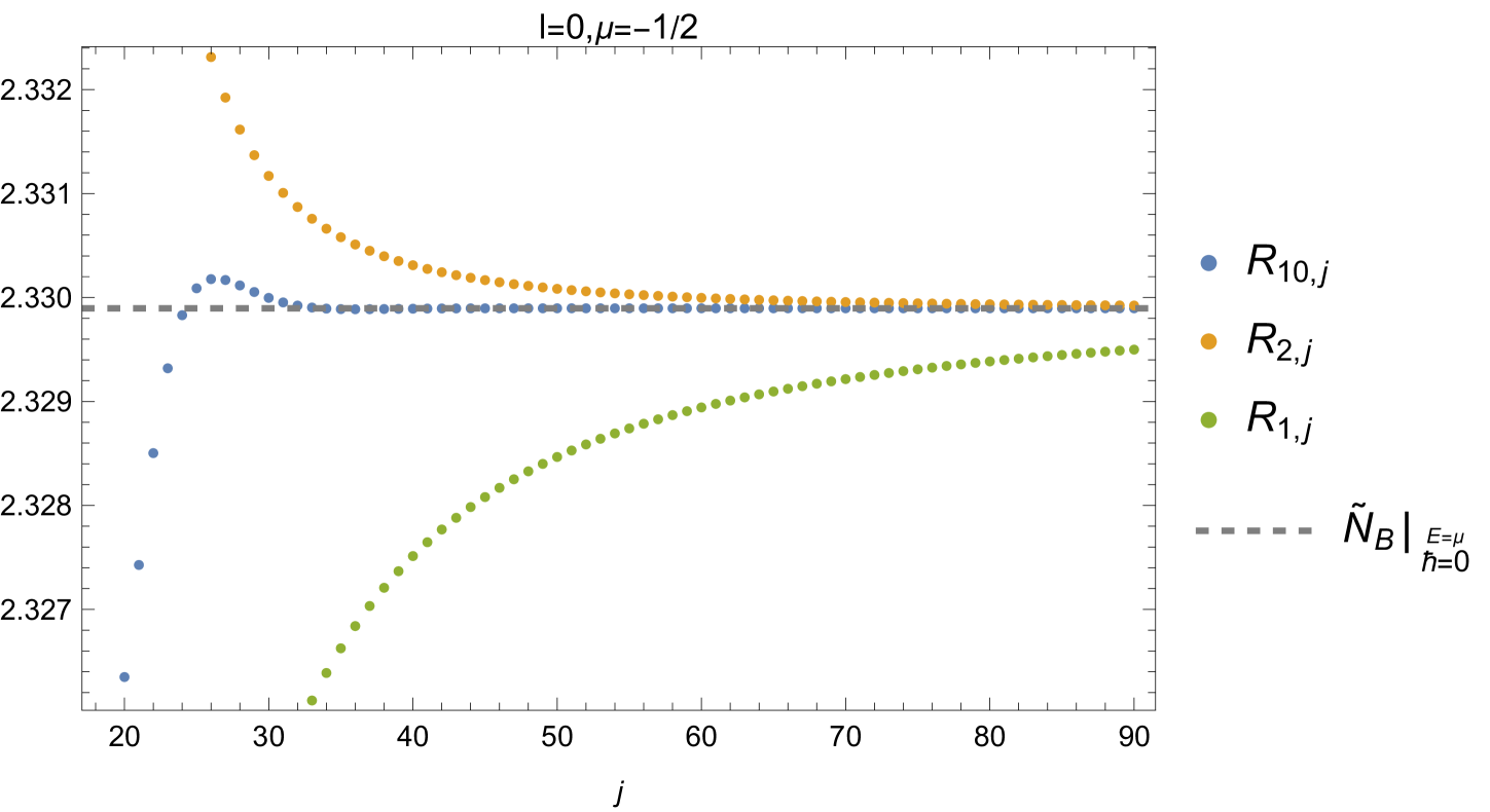
Figure 3: The plot shows the convergence acceleration provided by Richardson extrapolation. The sequences $R_{i,j}$ are the $i$th order Richardson of the ratio $r_{j}$ defined by (76). The gray dashed line is $N_{B}\lvert_{\hbar=0,E=\mu}$.

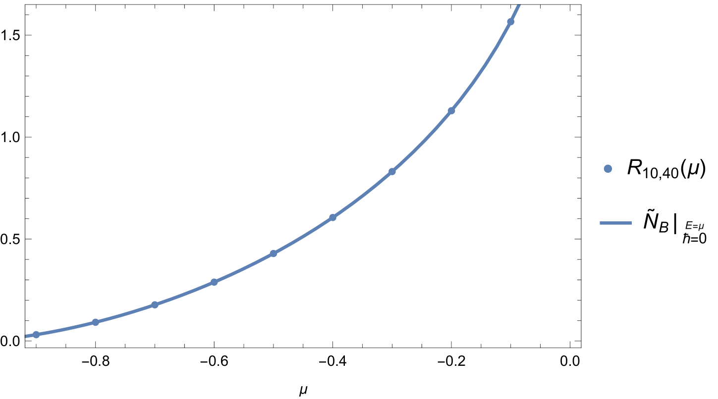
Figure 4: The sequence $R_{10,40}$ is the $10$th order Richardson extrapolation of the ratio $r_{j}$ defined by (76) evaluated at $j=40$. The solid blue curve is $\tilde{N}_{B}\lvert_{\hbar=0,E=\mu}=S(\mu)$ given by equation (73).

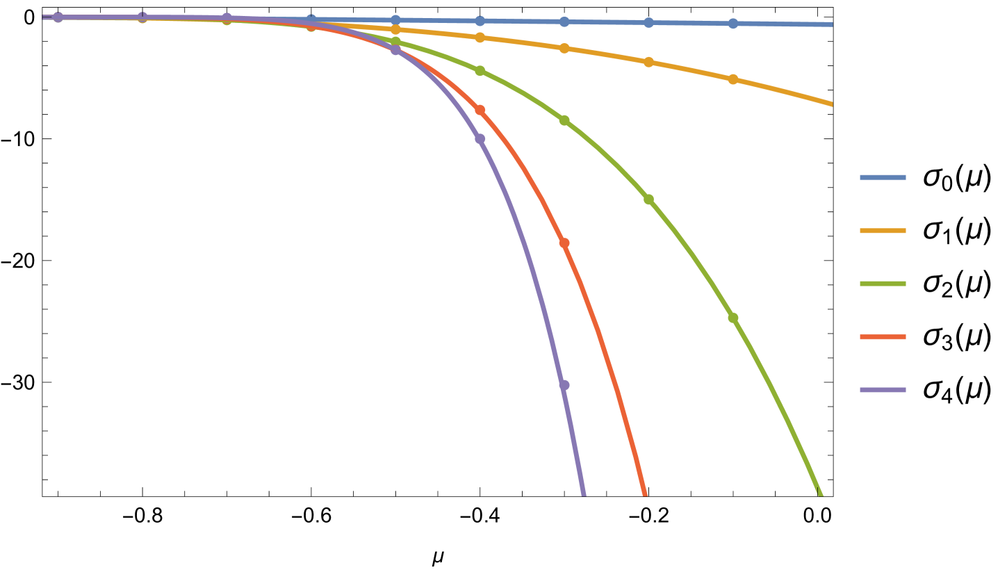
Figure 5: The plot shows the numerically calculated and exact Stokes constant given by $\sigma_{l}(\mu)$ defined in equation (71). The dots are the numerically calculated values while the solid lines are the exact values. The blue, orange, green, red and purple correspond to $l=0,1,2,3,4$ respectively. Each numeric approximation used 50 perturbative coefficients and Richardson acceleration of order 10.

In addition, the fluctuation coefficients were calculated by applying equation (69) iteratively. These numeric calculations were done for $j=1,2,3,4$ and are illustrated in figures 6, 7, 8 and 9. The agreement between the numeric calculations and the exact fluctuation series (70) confirms the proposed non-perturbative structure.

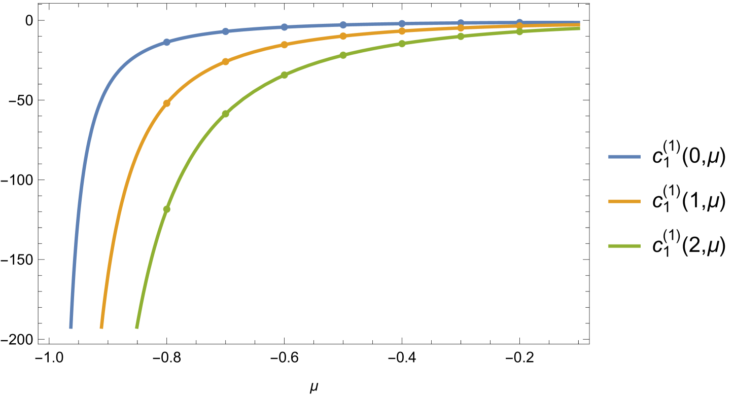
Figure 6: The plot shows the numerical and exact fluctuation coefficient $c^{(1)}_{1}(l,\mu)$. The dots are the numerically calculated values while the solid lines are the exact prediction. The blue, orange and green correspond to $l=0,1,2$ respectively. Each numeric approximation used 100 series coefficients and Richardson acceleration of order 10.

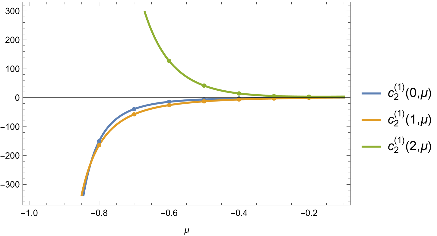
Figure 7: The plot shows the numerical and exact fluctuation coefficient $c^{(1)}_{2}(l,\mu)$. The dots are the numerically calculated values while the solid lines are the exact prediction. The blue, orange, and green correspond to $l=0,1,2$ respectively. Each numeric approximation used 100 series coefficients and Richardson acceleration of order 10.

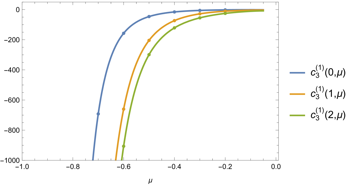
Figure 8: The plot shows the numerical and exact fluctuation coefficient $c^{(1)}_{3}(l,\mu)$. The dots are the numerically calculated values while the solid lines are the exact prediction. The blue, orange, and green correspond to $l=0,1,2$ respectively. Each numeric approximation used 100 series coefficients and Richardson acceleration of order 10.

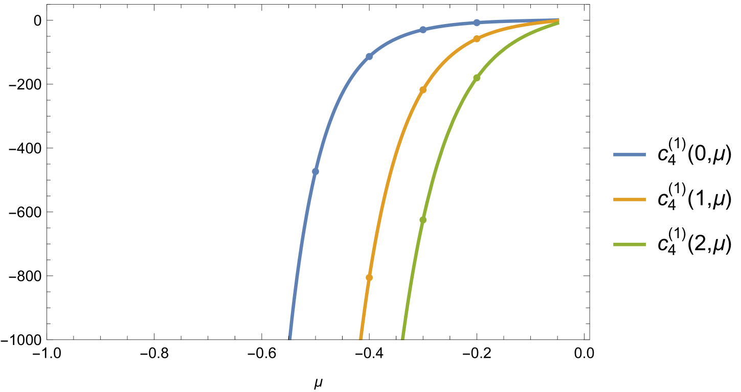
Figure 9: The plot shows the numerical and exact fluctuation coefficient $c^{(1)}_{4}(l,\mu)$. The dots are the numerically calculated values while the solid lines are the exact prediction. The blue, orange, and green correspond to $l=0,1,2$ respectively. Each numeric approximation used 100 series coefficients and Richardson acceleration of order 10.

5 Conclusion

The analysis presented above provides new non-perturbative results for the spheroidal eigenvalues as well as a parametric-resurgent analysis of the perturbative spectral data. We provided an algorithmic approach to the calculation of the quantum actions as well as a novel analysis of the P/NP relation that they satisfy. Finally, we presented a numerical Resurgent analysis which verified our results.

There are several directions for future research: (1) Analyze the interplay between the perturbative and non-perturbative structures of the eigenvalues for various regions of parameters, including inverting the potential, $\hbar\mapsto i\hbar$, as well as rotating to the imaginary axis, $x\mapsto ix$. (2) Developing exact quantization conditions and solving them with both TBA methods as well as transseries. (3) Generalize the analysis to treat the spin weighted spheroidal equation. (4) Study the non-perturbative structures in the quasinormal modes of Kerr and Kerr-Newman black holes where the spheroidal eigenvalues play a fundamental role Aminov2020 ; TeukolskyThesis ; silva2025kerrnewmanquasinormalmodesseibergwitten .

6 Acknowledgements

This work is supported in part by the U.S. Department of Energy, Office of High Energy Physics, Award DE-SC0010339. The author would like to thank Gerald Dunne for many insightful comments and valuable feedback.

Appendix A The complete Ellitpic integrals

The complete ellitpic integrals $\mathbf{K},\mathbf{E}$ and $\mathbf{\Pi}$ are defined as follows

$$\mathbf{K}(k)=\int_{0}^{1}\frac{dz}{\sqrt{(1-z^{2})(1-k^{2}z^{2})}},$$ (77)

$$\mathbf{E}(k)=\int_{0}^{1}\sqrt{\frac{1-k^{2}z^{2}}{1-z^{2}}}dz,$$

$$\mathbf{\Pi}(\nu,k)=\int_{0}^{1}\frac{dz}{(1-\nu z^{2})\sqrt{(1-z^{2})(1-k^{2}z^{2})}}.$$

They satsify the following differential equations NIST:DLMF :

$$\left(k^{2}-1\right)\frac{\partial^{2}\mathbf{\Pi}}{\partial k^{2}}+\frac{\left(3k^{4}+\left(-\nu-1\right)k^{2}-\nu\right)}{k\left(k^{2}-\nu\right)}\frac{\partial\mathbf{\Pi}}{\partial k}-\frac{2\left(-1+\nu\right)\nu}{k^{2}-\nu}\frac{\partial\mathbf{\Pi}}{\partial\nu}+\mathbf{\Pi}=0,$$ (78)

$$\frac{\left(k^{2}-\nu\right)}{k}\frac{\partial^{2}\mathbf{\Pi}}{\partial\nu\partial k}-\frac{1}{k}\frac{\partial^{2}\mathbf{\Pi}}{\partial\nu^{2}}+\frac{\partial\mathbf{\Pi}}{\partial\nu}=0,$$

$$\left(k^{2}-1\right)\frac{d^{2}\mathbf{K}}{dk^{2}}+\frac{\left(3k^{2}-1\right)}{k}\frac{d\mathbf{K}}{dk}+\mathbf{K}=0,$$

$$\left(k^{2}-1\right)\frac{d^{2}\mathbf{E}}{dk^{2}}+\frac{\left(1-k^{2}\right)}{k}\frac{d\mathbf{E}}{dk}+\mathbf{E}=0.$$

Appendix B The Differential Operator

The differential operator of equation (28) can be written

$$\mathcal{L}_{E,\mu}=q_{0}(E,\mu)+q_{E}(E,\mu)\partialderivative{E}+q_{\mu}(E,\mu)\partialderivative{\mu}$$ (79)

where $q_{0},q_{E}$ and $q_{\mu}$ are given by up to order $\hbar^{8}$ by the following three expressions:

$$q_{0}(E,\mu)=1+\hbar^{2}\left(\frac{1-E}{12(4\mu+(E-1)^{2})}+\frac{1}{48\mu-48E}\right)$$ (80)

$$+\hbar^{4}\Bigg{(}\frac{-15E^{2}+92E-33}{7680\left(E+1\right)^{3}(\mu-E)}+\frac{101E^{3}+57E^{2}-113E-45}{960(E+1)\left(4\mu+(E-1)^{2}\right)^{2}}+\frac{-7E^{4}+14E^{3}-14E+7}{90\left(4\mu+(E-1)^{2}\right)^{3}}$$

$$+\frac{-25E^{4}-50E^{3}-76E^{2}+90E+1}{960(E-1)(E+1)^{3}\left(4\mu+(E-1)^{2}\right)}+\frac{-7E-7}{2880(\mu-E)^{3}}+\frac{-34E-11}{7680(E+1)(\mu-E)^{2}}+\frac{1}{512\mu(E-1)}\Bigg{)}$$

$$+\hbar^{6}\Bigg{(}-\frac{1}{8192\mu^{2}(E-1)}+\frac{5-E}{24576\mu(E-1)^{3}}+\frac{31E^{2}+62E+31}{20160(\mu-E)^{5}}+\frac{3256E^{2}-3000E+3933}{2580480\left(E+1\right)^{2}(\mu-E)^{3}}$$

$$+\frac{210E^{3}-4715E^{2}+7424E-11327}{2580480\left(E+1\right)^{4}(\mu-E)^{2}}+\frac{35E^{4}+5964E^{3}-36066E^{2}+21764E+10559}{860160(E+1)^{6}(\mu-E)}$$

$$+\frac{4425E^{5}-8549E^{4}+1042E^{3}+3918E^{2}+1109E-1945}{5040\left(4\mu+(E-1)^{2}\right)^{4}}$$

$$+\frac{-97917E^{5}-95727E^{4}+85758E^{3}+110082E^{2}-11089E+8893}{161280(E+1)^{2}\left(4\mu+(E-1)^{2}\right)^{3}}$$

$$+\frac{19773E^{6}+53598E^{5}+18015E^{4}-13648E^{3}-102181E^{2}+25306E+2497}{161280(E-1)(E+1)^{4}\left(4\mu+(E-1)^{2}\right)^{2}}$$

$$+\frac{-364E^{6}+3333E^{5}-9359E^{4}+10370E^{3}-4506E^{2}-683E+649}{13440(E-1)^{3}(E+1)^{6}\left(4\mu+(E-1)^{2}\right)}$$

$$+\frac{-124E^{7}+372E^{6}-124E^{5}-620E^{4}+620E^{3}+124E^{2}-372E+124}{315\left(4\mu+(E-1)^{2}\right)^{5}}+\frac{914E+1031}{322560(\mu-E)^{4}}\Bigg{)},$$

(81)

$$q_{E}(E,\mu)=\hbar^{2}\left(\frac{(E-1)^{2}}{12\left(4\mu+(E-1)^{2}\right)}-\frac{E}{24(\mu-E)}+\frac{1}{12}\right)+\hbar^{4}\Bigg{(}\frac{102E^{2}+61E+28}{11520(E+1)(\mu-E)^{2}}$$

$$+\frac{E^{4}+18E^{2}-8E+1}{192(E+1)^{3}\left(4\mu+(E-1)^{2}\right)}+\frac{3E^{3}-15E^{2}+9E-1}{768(E+1)^{3}(\mu-E)}+\frac{-247E^{4}+20E^{3}+510E^{2}-92E-191}{2880(E+1)\left(4\mu+(E-1)^{2}\right)^{2}}$$

$$+\frac{7E^{5}-21E^{4}+14E^{3}+14E^{2}-21E+7}{90\left(4\mu+(E-1)^{2}\right)^{3}}+\frac{7E(E+1)}{1440(\mu-E)^{3}}-\frac{1}{256\mu}\Bigg{)}+\hbar^{6}\Bigg{(}\frac{1}{4096\mu^{2}}$$

$$+\frac{E-3}{\mu 12288\left(E-1\right)^{2}}+\frac{-914E^{2}-1279E-248}{161280(\mu-E)^{4}}-\frac{31E(E+1)^{2}}{10080(\mu-E)^{5}}$$

$$+\frac{-3256E^{3}-656E^{2}-9481E-1892}{1290240\left(E+1\right)^{2}(\mu-E)^{3}}+\frac{-210E^{4}+3087E^{3}-3439E^{2}+14777E-2163}{1290240(E+1)^{4}(\mu-E)^{2}}$$

$$+\frac{-105E^{5}-17997E^{4}+112282E^{3}-75414E^{2}-35313E+10675}{1290240(E+1)^{6}(\mu-E)}$$

$$+\frac{66981E^{6}+12946E^{5}-99109E^{4}-64004E^{3}+58635E^{2}+4562E+19989}{\left(E+1\right)^{2}\left(4\mu+(E-1)^{2}\right)^{3}}$$

$$+\frac{-1416E^{6}-2790E^{5}+6729E^{4}-23236E^{3}+27016E^{2}-6602E-1381}{80640(E+1)^{4}\left(4\mu+(E-1)^{2}\right)^{2}}$$

$$+\frac{-3929E^{6}+10990E^{5}-7111E^{4}-2876E^{3}+329E^{2}+5038E-2441}{5040\left(4\mu+(E-1)^{2}\right)^{4}}$$

$$+\frac{124E^{8}-496E^{7}+496E^{6}+496E^{5}-1240E^{4}+496E^{3}+496E^{2}-496E+124}{315\left(4\mu+(E-1)^{2}\right)^{5}}$$

$$+\frac{-1845E^{8}-7380E^{7}+1356E^{6}-66548E^{5}+178750E^{4}-104156E^{3}-8276E^{2}+21844E-7025}{161280\left(E-1\right)(E+1)^{6}\left(4\mu+(E-1)^{2}\right)}\Bigg{)},$$

(82)

$$q_{m}(E,\mu)=\hbar^{2}\left(\frac{E}{24}+\frac{1}{24}-\frac{(E-1)^{3}}{24\left(4\mu+(E-1)^{2}\right)}-\frac{E}{24(\mu-E)}\right)+\hbar^{4}\Bigg{(}\frac{158E^{2}+145E+56}{(11520E+11520)(\mu-E)^{2}}$$

$$+\frac{49E^{3}-13E^{2}+89E+11}{3840(E+1)^{3}(\mu-E)}+\frac{-7E^{6}+28E^{5}-35E^{4}+35E^{2}-28E+7}{180\left(4\mu+(E-1)^{2}\right)^{3}}+\frac{7E(E+1)}{1440(\mu-E)^{3}}-\frac{1}{256\mu}+\frac{5}{384}$$

$$+\frac{527E^{5}-659E^{4}-826E^{3}+1162E^{2}+155E-359}{5760(E+1)\left(4\mu+(E-1)^{2}\right)^{2}}+\frac{-63E^{5}-142E^{4}-64E^{3}+190E^{2}+57E+22}{960(E+1)^{3}\left(4\mu+(E-1)^{2}\right)}\Bigg{)}$$

$$+\frac{\hbar^{6}}{1290240}\Bigg{(}\frac{315}{\mu^{2}}+\frac{128\left(6409E^{2}+8694E+3929\right)(E-1)^{5}}{\left(4\mu+(E-1)^{2}\right)^{4}}-\frac{8\left(1410E^{2}+2023E+496\right)}{(\mu-E)^{4}}$$

$$+\frac{10568E^{3}+19872E^{2}+27741E+8248}{(E+1)^{2}(E-\mu)^{3}}-\frac{3968E(E+1)^{2}}{(\mu-E)^{5}}-\frac{315}{\mu-\mu E}-\frac{253952(E+1)^{2}(E-1)^{7}}{\left(4\mu+(E-1)^{2}\right)^{5}}$$

$$-\frac{4\left(239517E^{4}+628076E^{3}+614190E^{2}+273516E+71133\right)(E-1)^{3}}{(E+1)^{2}\left(4\mu+(E-1)^{2}\right)^{3}}$$

$$+\frac{-3466E^{4}+1203E^{3}-8613E^{2}+6461E-3933}{(E+1)^{4}(\mu-E)^{2}}$$

$$+\frac{-315E^{5}-13597E^{4}+109994E^{3}-64098E^{2}-16447E+11327}{(E+1)^{6}(\mu-E)}$$

$$+\frac{8\left(58845E^{7}+162693E^{6}+84015E^{5}-108767E^{4}-191683E^{3}+15345E^{2}-14753E-5695\right)}{(E+1)^{4}\left(4\mu+(E-1)^{2}\right)^{2}}$$

$$-\frac{4\left(19773E^{8}+93144E^{7}+149352E^{6}+35984E^{5}+846E^{4}-317144E^{3}+5000E^{2}+38496E-5291\right)}{(E-1)(E+1)^{6}\left(4\mu+(E-1)^{2}\right)}\Bigg{)},$$

Appendix C The Fluctuation Coefficients

The first three of the calculated fluctuation coefficients defined in (70) are listed below

$$c^{(1)}_{0} =0,$$ (83)

$$c^{(1)}_{1} =\frac{7\mu\left(l+\frac{1}{2}\right)^{2}}{4\sqrt{2}(\mu+1)^{3/2}}-\frac{3\left(l+\frac{1}{2}\right)^{2}}{8\sqrt{2}(\mu+1)^{3/2}}+\frac{\mu\left(l+\frac{1}{2}\right)}{\sqrt{2}(\mu+1)^{3/2}}-\frac{l+\frac{1}{2}}{2\sqrt{2}(\mu+1)^{3/2}}$$

$$-\frac{11}{32\sqrt{2}(\mu+1)^{3/2}}+\frac{17\mu}{48\sqrt{2}(\mu+1)^{3/2}}-\frac{i\pi}{8\sqrt{2}\sqrt{\mu}}+\frac{\text{arcsinh}\left(\sqrt{\mu}\right)}{4\sqrt{2}\sqrt{\mu}},$$

$$c^{(1)}_{2} =\frac{1}{18432\sqrt{2}\mu(\mu+1)^{5/2}}\Bigg{(}\Big{(}24i\pi\sqrt{\mu}\sqrt{\mu+1}(33-\mu-34\mu^{2})-144\pi^{2}(\mu+1)^{3}$$

$$+(4\mu(865\mu+4623)+225)\mu\Big{)}+48\sqrt{\mu}\Big{(}\sqrt{\mu}(4\mu(37\mu+367)+15)$$

$$-24i\pi\sqrt{\mu+1}\left(2\mu^{2}+\mu-1\right)\Big{)}\left(l+\frac{1}{2}\right)+24\sqrt{\mu}\Big{(}(4\mu(119\mu+435)-45)\sqrt{\mu}$$

$$-12i\pi(\mu+1)^{3/2}(14\mu-3)\Big{)}\left(l+\frac{1}{2}\right)^{2}+576\mu(12\mu(3\mu+5)+1)\left(l+\frac{1}{2}\right)^{3}$$

$$+144(3-14\mu)^{2}\mu\left(l+\frac{1}{2}\right)^{4}\Bigg{)}+\Bigg{(}\frac{1}{384\sqrt{2}\mu}\left(\frac{\sqrt{\mu}(34\mu-33)}{\mu+1}-12i\pi\sqrt{\mu+1}\right)$$

$$+\frac{2\mu-1}{8\sqrt{2}\sqrt{\mu}(\mu+1)}\left(l+\frac{1}{2}\right)+\frac{14\mu-3}{32\sqrt{2}\sqrt{\mu}(\mu+1)}\left(l+\frac{1}{2}\right)^{2}\Bigg{)}\text{ arcsinh}(\sqrt{\mu})$$

$$+\frac{\sqrt{\mu+1}\text{ arcsinh}\left(\sqrt{\mu}\right)^{2}}{32\sqrt{2}\mu}$$

References

- (1) F.A. Grünbaum, Serendipity strikes again, Proceedings of the National Academy of Sciences 119 (2022) e2207652119 [https://www.pnas.org/doi/pdf/10.1073/pnas.2207652119].
- (2) D. Slepian, Some comments on fourier analysis, uncertainty and modeling, SIAM Review 25 (1983) 379.
- (3) D. Slepian and H.O. Pollak, Prolate spheroidal wave functions, fourier analysis and uncertainty — I, The Bell System Technical Journal 40 (1961) 43.
- (4) H.J. Landau and H.O. Pollak, Prolate spheroidal wave functions, fourier analysis and uncertainty — II, The Bell System Technical Journal 40 (1961) 65.
- (5) F.A. Grünbaum, Commuting integral and differential operators and the master symmetries of the Korteweg-de Vries equation, Inverse Problems 37 (2021) 085010.
- (6) R. Longo, Signal Communication and Modular Theory, Commun. Math. Phys. 403 (2023) 473 [2302.13842].
- (7) A. Connes, Trace formula in noncommutative geometry and the zeros of the Riemann zeta function, Selecta Mathematica 5 (1999) 29.
- (8) A. Connes and M. Marcolli, Noncommutative geometry, quantum fields and motives, American Mathematical Society colloquium publications, vol. 55, American Mathematical Society, Providence, R.I (2008).
- (9) F. Fauvet, J.-P. Ramis, F. Richard-Jung and J. Thomann, Stokes phenomenon for the prolate spheroidal wave equation, Applied numerical mathematics 60 (2010) 1309.
- (10) F. Richard-Jung, J.-P. Ramis, J. Thomann and F. Fauvet, New Characterizations for the Eigenvalues of the Prolate Spheroidal Wave Equation, Studies in Applied Mathematics 138 (2017) 3 [https://onlinelibrary.wiley.com/doi/pdf/10.1111/sapm.12134].
- (11) A. Connes and H. Moscovici, The UV prolate spectrum matches the zeros of zeta, Proceedings of the National Academy of Sciences 119 (2022) e2123174119 [https://www.pnas.org/doi/pdf/10.1073/pnas.2123174119].
- (12) A. Connes and C. Consani, Spectral Triples and Zeta-Cycles, Enseign. Math. 69 (2023) [2106.01715].
- (13) A. Connes, C. Consani and H. Moscovici, Zeta zeros and prolate wave operators, 2024.
- (14) M.-Y. Choi, Y.-H. Hyun and Y. Kim, Angle dependence of the Landau level spectrum in twisted bilayer graphene, Physical review. B, Condensed matter and materials physics 84 (2011) .
- (15) Y.-H. Hyun, Y. Kim, C. Sochichiu and M.-Y. Choi, Landau level spectrum for bilayer graphene in a tilted magnetic field, Journal of Physics: Condensed Matter 24 (2012) 045501.
- (16) R. de Gail, M.O. Goerbig, F. Guinea, G. Montambaux and A.H. Castro Neto, Topologically protected zero modes in twisted bilayer graphene, Phys. Rev. B 84 (2011) 045436.
- (17) S. Becker, J. Kim and X. Zhu, Magnetic Response Properties of Twisted Bilayer Graphene, Annales Henri Poincaré (2024) .
- (18) H.J. Müller, Asymptotic Expansions of Prolate Spheriodial Wave Functions and their Characteristic Numbers, Journal für die reine und angewandte Mathematik 1963 (1963) 26.
- (19) S. Teukolsky, Perturbations of a Rotating Black Hole, Ph.D. thesis, California Institute of Technology, 1974.
- (20) E.W. Leaver and S. Chandrasekhar, An analytic representation for the quasi-normal modes of Kerr black holes, Proceedings of the Royal Society of London. A. Mathematical and Physical Sciences 402 (1985) 285 [https://royalsocietypublishing.org/doi/pdf/10.1098/rspa.1985.0119].
- (21) E. Berti, V. Cardoso and A.O. Starinets, Quasinormal modes of black holes and black branes, Classical and Quantum Gravity 26 (2009) 163001.
- (22) S. Iyer and C.M. Will, Black-hole normal modes: A WKB approach. I. Foundations and application of a higher-order WKB analysis of potential-barrier scattering, Phys. Rev. D 35 (1987) 3621.
- (23) E. Seidel and S. Iyer, Black-hole normal modes: A WKB approach. IV. Kerr black holes, Phys. Rev. D 41 (1990) 374.
- (24) H. Yang, F. Zhang, A. Zimmerman, D.A. Nichols, E. Berti and Y. Chen, Branching of quasinormal modes for nearly extremal Kerr black holes, Physical Review D 87 (2013) .
- (25) R.A. Konoplya, Quasinormal behavior of the d-dimensional Schwarzschild black hole and higher order WKB approach, Phys. Rev. D 68 (2003) 024018 [gr-qc/0303052].
- (26) R.A. Konoplya, A. Zhidenko and A.F. Zinhailo, Higher order WKB formula for quasinormal modes and grey-body factors: recipes for quick and accurate calculations, Class. Quant. Grav. 36 (2019) 155002 [1904.10333].
- (27) R.A. Konoplya and A. Zhidenko, Analytic expressions for quasinormal modes and grey-body factors in the eikonal limit and beyond, Class. Quant. Grav. 40 (2023) 245005 [2309.02560].
- (28) J. Matyjasek and M. Opala, Quasinormal modes of black holes: The improved semianalytic approach, Physical Review D 96 (2017) .
- (29) H. Yang, D.A. Nichols, F. Zhang, A. Zimmerman, Z. Zhang and Y. Chen, Quasinormal-mode spectrum of Kerr black holes and its geometric interpretation, Phys. Rev. D 86 (2012) 104006.
- (30) S. Iyer, Black-hole normal modes: A WKB approach. II. Schwarzschild black holes, Phys. Rev. D 35 (1987) 3632.
- (31) K.D. Kokkotas and B.F. Schutz, Black-hole normal modes: A WKB approach. III. The Reissner-Nordström black hole, Phys. Rev. D 37 (1988) 3378.
- (32) R.A. Konoplya, Quasinormal behavior of the D-dimensional Schwarzschild black hole and the higher order WKB approach, Physical Review D 68 (2003) .
- (33) K. Imaizumi, Quasi-normal modes for the D3-branes and Exact WKB analysis, Physics Letters B 834 (2022) 137450.
- (34) K. Imaizumi, Exact conditions for quasi-normal modes of extremal M5-branes and exact WKB analysis, Nucl. Phys. B 992 (2023) 116221 [2212.04738].
- (35) O. Costin and G.V. Dunne, Physical Resurgent Extrapolation, Phys. Lett. B 808 (2020) 135627 [2003.07451].
- (36) D. Fioravanti, D. Gregori and H. Shu, Integrability, susy matter gauge theories and black holes, 2022.
- (37) D. Fioravanti and D. Gregori, A new method for exact results on Quasinormal Modes of Black Holes, 2022.
- (38) G. Aminov, A. Grassi and Y. Hatsuda, Black Hole Quasinormal Modes and Seiberg-Witten Theory, Annales Henri Poincare 23 (2022) 1951 [2006.06111].
- (39) G. Bonelli, C. Iossa, D.P. Lichtig and A. Tanzini, Exact solution of Kerr black hole perturbations via CFT2 and instanton counting: Greybody factor, quasinormal modes, and Love numbers, Phys. Rev. D 105 (2022) 044047 [2105.04483].
- (40) M. Bianchi, D. Consoli, A. Grillo and J.F. Morales, More on the SW-QNM correspondence, Journal of High Energy Physics 2022 (2022) 24.
- (41) G. Aminov, P. Arnaudo, G. Bonelli, A. Grassi and A. Tanzini, Black hole perturbation theory and multiple polylogarithms, JHEP 11 (2023) 059 [2307.10141].
- (42) P. Arnaudo, G. Bonelli and A. Tanzini, One loop effective actions in Kerr-(A)dS black holes, Phys. Rev. D 110 (2024) 106006 [2405.13830].
- (43) P. Arnaudo, G. Bonelli and A. Tanzini, One-loop corrections to near extremal Kerr thermodynamics from semiclassical Virasoro blocks, 2412.16057.
- (44) Y. Hatsuda and M. Kimura, Spectral Problems for Quasinormal Modes of Black Holes, Universe 7 (2021) 476 [2111.15197].
- (45) Y. Hatsuda, Quasinormal modes of black holes and Borel summation, Phys. Rev. D 101 (2020) .
- (46) Y. Hatsuda, An alternative to the Teukolsky equation, General Relativity and Gravitation 53 (2021) .
- (47) H.O. Silva, J.-W. Kim and M.V.S. Saketh, Kerr-Newman quasinormal modes and Seiberg-Witten theory, 2502.17488.
- (48) R.S. Borissov and P.P. Fiziev, Exact Solutions of Teukolsky Master Equation with Continuous Spectrum, Bulg. J. Phys. 37 (2010) 065 [0903.3617].
- (49) Y.F. Bautista, G. Bonelli, C. Iossa, A. Tanzini and Z. Zhou, Black hole perturbation theory meets CFT2: Kerr-Compton amplitudes from Nekrasov-Shatashvili functions, Phys. Rev. D 109 (2024) 084071 [2312.05965].
- (50) J.L. Dunham, The Wentzel-Brillouin-Kramers Method of Solving the Wave Equation, Phys. Rev. 41 (1932) 713.
- (51) A. Voros, The return of the quartic oscillator. The complex WKB method, Annales de l’I.H.P. Physique théorique 39 (1983) 211.
- (52) É. Delabaere, H. Dillinger and F. Pham, Exact semiclassical expansions for one-dimensional quantum oscillators, J. Math. Phys. 38 (1997) 6126.
- (53) B. Bucciotti, T. Reis and M. Serone, An anharmonic alliance: exact WKB meets EPT, JHEP 11 (2023) 124 [2309.02505].
- (54) A. van Spaendonck and M. Vonk, Exact instanton transseries for quantum mechanics, SciPost Physics 16 (2024) .
- (55) A. Grassi, Q. Hao and A. Neitzke, Exact WKB methods in SU(2) nf = 1, Journal of High Energy Physics 2022 (2022) .
- (56) F. Yan, Exact WKB and the quantum Seiberg-Witten curve for 4d N = 2 pure SU(3) Yang-Mills. Abelianization, JHEP 03 (2022) 164 [2012.15658].
- (57) I. Coman, P. Longhi and J. Teschner, From Quantum Curves to Topological String Partition Functions II, Annales Henri Poincaré (2025) .
- (58) K. Imaizumi, Exact WKB analysis and TBA equations for the Mathieu equation, Physics Letters B 806 (2020) 135500.
- (59) K. Imaizumi, Quantum periods and TBA equations for N=2 SU(2) Nf=2 SQCD with flavor symmetry, Physics Letters B 816 (2021) 136270.
- (60) Y. Emery, TBA equations and quantization conditions, Journal of High Energy Physics 2021 (2021) .
- (61) K. Ito, M. Mariño and H. Shu, TBA equations and resurgent Quantum Mechanics, JHEP (2019) .
- (62) K. Ito and J. Yang, Exact WKB analysis and TBA equations for the Stark effect, Prog. Theor. Exp. Phys. (2024) Paper No. 013A02, 30.
- (63) P. Dorey and R. Tateo, Anharmonic oscillators, the thermodynamic Bethe ansatz and nonlinear integral equations, Journal of Physics A: Mathematical and General 32 (1999) L419–L425.
- (64) P. Lo Chiatto, S. Schenk and F. Yu, Quantum Imprint of the Anharmonic Oscillator, 2308.01244.
- (65) R. Hwa and V. Teplitz, Homology and Feynman Integrals, Mathematical physics monograph series, W. A. Benjamin, New York (1966).
- (66) G. Başar, G.V. Dunne and M. Ünsal, Quantum geometry of resurgent perturbative/nonperturbative relations, Journal of High Energy Physics (2017) .
- (67) M. Raman and P.N.B. Subramanian, On Chebyshev Wells: Periods, Deformations, and Resurgence, Phys. Rev. D 101 (2020) 126014.
- (68) F. Fischbach, A. Klemm and C. Nega, WKB Method and Quantum Periods beyond Genus One, Journal of Physics A: Mathematical and Theoretical 52 (2019) 075402.
- (69) M. Meynig, Generating and Computing Quantum Periods in Exact WKB, 2412.20643.
- (70) P.A. Griffiths, On the Periods of Certain Rational Integrals: I, Ann. Math. 90 (1969) 460.
- (71) P.A. Griffiths, The residue calculus and some transcendental results in algebraic geometry I, Proceedings of the National Academy of Sciences 55 (1966) 1303 [https://www.pnas.org/doi/pdf/10.1073/pnas.55.5.1303].
- (72) D. Cox and S. Katz, Mirror Symmetry and Algebraic Geometry, Mathematical Surveys and Monographs, American Mathematical Society, United States (1999), 10.1090/surv/068.
- (73) P. Lairez, Computing periods of rational integrals, Math. Comput. 85 (2015) 1719–1752.
- (74) S. Müller-Stach, S. Weinzierl and R. Zayadeh, Picard-Fuchs equations for Feynman integrals, Commun. Math. Phys. 326 (2014) 237–249.
- (75) D.R. Morrison, Picard-Fuchs equations and mirror maps for hypersurfaces, AMS/IP Stud. Adv. Math. 9 (1998) 185 [hep-th/9111025].
- (76) P. Lairez and P. Vanhove, Algorithms for minimal Picard–Fuchs operators of Feynman integrals, Lett. Math. Phys. 113 (2023) 37.
- (77) A. Çavuşoğlu, C. Kozçaz and K. Tezgin, Unified genus-1 potential and parametric P/NP relation, 2311.17850.
- (78) T. Sulejmanpasic and M. Ünsal, Aspects of perturbation theory in quantum mechanics: The BenderWu Mathematica ® package, Computer Physics Communications 228 (2018) 273.
- (79) G. Başar and G.V. Dunne, Resurgence and the Nekrasov-Shatashvili limit: connecting weak and strong coupling in the Mathieu and Lamé systems, JHEP 02 (2015) 160 [1501.05671].
- (80) G. Álvarez and C. Casares, Exponentially small corrections in the asymptotic expansion of the eigenvalues of the cubic anharmonic oscillator, Journal of Physics A: Mathematical and General 33 (2000) 5171.
- (81) A. Çavuşoğlu, C. Kozşaz and K. Tezgin, Resurgence of Deformed Genus-1 Curves: A Novel P/NP Relation, 2024.
- (82) B. Eynard, Lectures notes on compact Riemann surfaces, 2018.
- (83) A. Gorsky and A. Milekhin, RG-Whitham dynamics and complex Hamiltonian systems, Nuclear Physics B 895 (2015) 33–63.
- (84) M. Matone, Instantons and recursion relations in N = 2 SUSY gauge theory, Physics Letters B 357 (1995) 342.
- (85) G.V. Dunne and M. Ünsal, Generating nonperturbative physics from perturbation theory, Physical Review D 89 (2014) .
- (86) A. Marshakov and A. Mironov, Seiberg-Witten Systems and Whitham Hierarchies: a Short Review, 1998.
- (87) O. Costin, Asymptotics and Borel Summability, Taylor and Francis (2008).
- (88) C.M. Bender and S.A. Orszag, Advanced mathematical methods for scientists and engineers, International series in pure and applied mathematics, McGraw-Hill, New York (1978).
- (89) H.O. Silva, J.-W. Kim and M.V.S. Saketh, Kerr-Newman quasinormal modes and Seiberg-Witten theory, 2025.
- (90) “NIST Digital Library of Mathematical Functions.” https://dlmf.nist.gov/, Release 1.2.3 of 2024-12-15.