Interaction-free ergodicity breaking in spherical model driven by temporally hyperuniform noise

Abstract

We investigate the effects of temporal hyperuniformity of driving forces in the spherical model. The spherical model with $p$-body random interactions is a prototypical model to investigate the ergodicity breaking of glass transitions, where the spin-spin interactions are key ingredients to cause the ergodicity breaking. However, for the model driven by temporally hyperuniform noise, the strong anticorrelation of the noise can solely cause an ergodicity breaking even without spin-spin interactions. Near the transition point, the static susceptibility and relaxation time show power-law divergence with a common critical exponent, which varies depending on the strength of hyperuniformity.

• April 5, 2025

1 Introduction

The concept of hyperuniformity was introduced by Torquato and Stillinger to represent anomalous suppression of large-scale fluctuations [1, 2]. Hyperuniformity is characterized by the power-law behavior of the structure factor $S(k)\sim\left|k\right|^{\alpha}$ with positive $\alpha$ for small wave vector $k$. Hyperuniformity was reported in various systems, including density fluctuations of crystals [3], quasicrystals [4, 5], amorphous solids [6, 7, 8, 9, 10, 11, 12], and several out-of-equilibrium systems [13, 14, 15, 16, 17, 18, 19, 20, 21, 22]. Torquato classified hyperuniformity depending on the value of $\alpha$ [1]. In particular, hyperuniformity with $\alpha>1$ is referred to as class I hyperuniformity and belongs to the strongest form of hyperuniformity in his classification [1].

The impact of hyperuniformity on various properties of systems has been actively investigated. Most previous studies have focused on hyperuniformity in spatial fluctuations of particle arrangements [6, 23, 8, 12], external field [24, 25, 26, 27], interactions [28, 26, 29], noise [13, 17, 18, 19, 20], and so on. In the context of active matter, such as chiral and pulsating active matter, the driving forces often undergo periodic oscillations in time [30, 31, 32]. The spectrum of those driving forces tends to zero as the frequency tends to zero, i.e., exhibits temporal hyperuniformity. The effect of temporal hyperuniformity has not yet been fully investigated [18]. Here, we show that temporally hyperuniform noise leads to a novel ergodicity breaking by using a simple mean-field spin model with a global spherical constraint.

The continuous spin model with the global spherical constraint is referred to as the spherical model and is widely applied to describe the ferromagnetic transition [33, 34], and the glass transitions [35, 36, 37]. In particular, the spherical model with disordered $p$-body interaction is known as the $p$-spin spherical model (PSM) and is recognized as a prototypical model to study the ergodicity breaking of structural glasses and spin-glasses [37, 38]. In equilibrium, the PSM exhibits the ergodicity breaking at a finite temperature, which is attributed to the competing spin-spin interactions. On the contrary, for the out-of-equilibrium model driven by temporally hyperuniform noise, we show that the ergodicity breaking can occur even without explicit spin-spin interactions.

The remainder of this paper is organized as follows. In Sec. 2, we introduce the model. In Sec. 3, we analyze the model in the ergodic phase. The analysis reveals that for the noise belonging to class I hyperuniform, the model has a finite critical point at which the static spin susceptibility and relaxation time diverge. The critical exponent near the transition point is determined, which varies depending on the strength of the hyperuniformity. In Sec. 4, we analyze the model in the non-ergodic phase. Finally, in Sec. 5, we conclude the work.

2 Model

We consider a system consisting of $N$ continuous spin variables: $\{\sigma_{1},\cdots,\sigma_{N}\}$, which satisfy a global spherical constraint [33, 37]:

$$\sum_{i=1}^{N}\sigma_{i}^{2}=N.$$ (1)

To impose the constraint, we consider the following potential:

$$H=\frac{\mu}{2}\sum_{i=1}^{N}\sigma_{i}^{2},$$ (2)

where $\mu$ denotes the Lagrange multiplier to impose the constraint. For the time evolution, we consider the following equation of motion (EOM):

$$\dot{\sigma}_{i}=-\frac{\partial H}{\partial\sigma_{i}}+\xi_{i}=-\mu\sigma_{i}+\xi_{i},$$ (3)

where $\xi_{i}(t)$ denotes a correlated noise with zero mean and variance:

$$\left\langle\xi_{i}(t)\xi_{j}(t^{\prime})\right\rangle=2\delta_{ij}TD(t),$$ (4)

where $T$ denotes the strength of the noise and plays the role of effective temperature. For the thermal white noise, $D(t)$ is a delta function, and its Fourier spectrum becomes constant. To introduce the effects of temporal hyperuniformity, we consider the following spectrum for the noise:

$$D(\omega)\equiv\int_{-\infty}^{\infty}dte^{i\omega t}D(t)=\begin{cases}\left|\omega/\omega_{0}\right|^{\alpha}&\left|\omega\right|\leq\omega_{0}\\ 1&\left|\omega\right|>\omega_{0}\end{cases},$$ (5)

where $\alpha$ and $\omega$ are some constants. In Fig. 1, we plot $D(\omega)$ for several $\alpha$. The white noise is recovered in the limit either $\omega_{0}\to 0$ or $\alpha\to 0$.

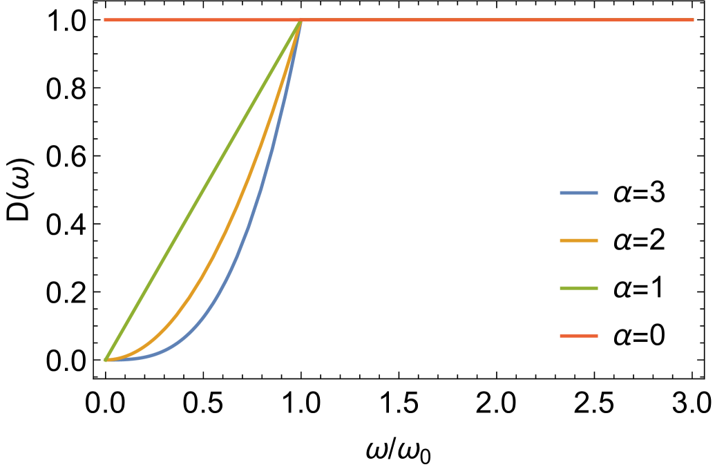
Figure 1: The spectrum of the noise $D(\omega)$ for several $\alpha$. The thermal white noise corresponds to $\alpha=0$. For $\alpha>0$, $D(\omega)$ vanishes in the limit of small frequency.

For $\alpha>0$, $D(\omega)\to 0$ in the limit of small $\omega$. This means that the fluctuations of the noise are highly suppressed in the long-time limit, i.e., the noise is temporally hyperuniform.

3 Ergodic phase

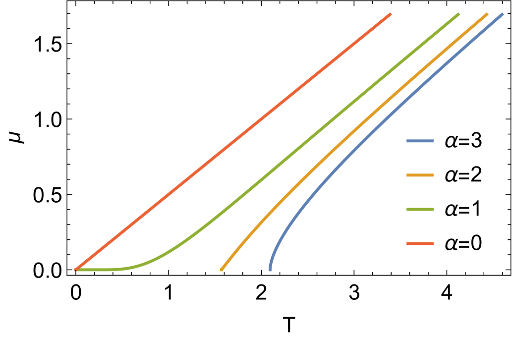
Figure 2: $T$ dependence of the Lagrange multiplier $\mu$ for various $\alpha$ and $\omega_{0}=1$. For $\alpha>1$, $\mu$ becomes zero at a finite noise strength $T_{c}$.

We investigate the model in the steady state, where $\mu$ does not depend on $t$. The EOM (3) in the frequency space leads to

$$\sigma_{i}(\omega)=\frac{\xi_{i}(\omega)}{i\omega+\mu}.$$ (6)

The two point correlation is then calculated as

$$\left\langle\sigma_{i}(\omega)\sigma_{i}(\omega^{\prime})\right\rangle=2\pi\delta(\omega+\omega^{\prime})C(\omega),$$ (7)

where

$$C(\omega)=\frac{TD(\omega)}{\omega^{2}+\mu^{2}}.$$ (8)

The equal time correlation is then

$$\left\langle\sigma_{i}(t)^{2}\right\rangle=\frac{1}{2\pi}\int d\omega C(\omega)=\frac{T}{\pi}\int_{0}^{\infty}d\omega\frac{D(\omega)}{\omega^{2}+\mu^{2}}.$$ (9)

The Lagrange multiplier $\mu$ is to be determined by the spherical constraint:

$$1=\frac{1}{N}\sum_{i=1}^{N}\left\langle\sigma_{i}(t)^{2}\right\rangle=\frac{T}{\pi}\int_{0}^{\infty}d\omega\frac{D(\omega)}{\omega^{2}+\mu^{2}}.$$ (10)

In Fig. 2, we show the $T$ dependence of the Lagrange multiplier $\mu$ obtained by numerically solving Eq. (10). For $\alpha>1$, the Lagrange multiplier $\mu$ vanishes at a finite critical temperature:

$$T_{c}=\pi\left[\int_{0}^{\infty}d\omega\frac{D(\omega)}{\omega^{2}}\right]^{-1}=\pi\omega_{0}\frac{\alpha-1}{\alpha}.$$ (11)

In Fig. 3, we show the $\alpha$ dependence of $T_{c}$ for various $\omega_{0}$.

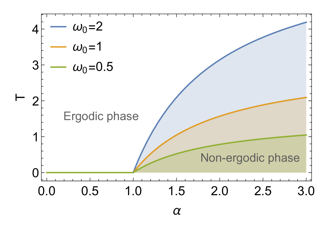
Figure 3: Phase diagrams for various $\omega_{0}$: The solid lines denote the critical temperatures $T_{c}$, and filled regions denote the non-ergodic phases. The transition point is finite $T_{c}>0$ for $\alpha>1$, and $T_{c}=0$ for $\alpha\leq 1$.

To characterize the criticality of the model, we investigate the linear response by introducing the external field: $H\to H+\sum_{i=1}^{N}h(t)\sigma_{i}(t)$ [39]. After some manipulations, we get

$$\left\langle\sigma_{i}(\omega)\right\rangle=G(\omega)h(\omega),$$ (12)

where the response function is

$$G(\omega)=\frac{1}{\mu+i\omega}.$$ (13)

The static spin susceptibility is then calculated as

$$\chi=\lim_{\omega\to 0}\frac{1}{N}\sum_{i=1}^{N}\frac{\left\langle\sigma_{i}(\omega)\right\rangle}{h(\omega)}=\lim_{\omega\to 0}G(\omega)=\frac{1}{\mu}.$$ (14)

The susceptibility diverges at $T_{c}$ as $\mu$ vanishes. The detailed scaling behavior of $\chi$ can be obtained by the asymptotic analysis of Eq. (10). For $\alpha\leq 1$, $\mu$ vanishes at $T=0$. The asymptotic analysis of Eq. (10) for $T\ll 1$ and $\mu\ll 1$ leads to

$$\chi \propto\begin{cases}T^{-\frac{1}{1-\alpha}}&\alpha<1,\\ e^{\frac{\pi}{T}}&\alpha=1.\end{cases}$$ (15)

The exponential divergence for $\alpha=1$ is similar to the behavior commonly observed at the lower critical dimension [39, 40]. In Fig. 4 (a), we also show the numerical results of $\chi$ for $\alpha\leq 1$ obtained by Eq. (10). For $\alpha>1$, the asymptotic analysis near $T_{c}$ for $\mu\ll 1$ leads to

$$\chi\propto\begin{cases}(T-T_{c})^{-\frac{1}{\alpha-1}}&1<\alpha<3\\ (T-T_{c})^{-\frac{1}{2}}\left[-\log(T-T_{c})\right]^{1/2}&\alpha=3\\ (T-T_{c})^{-\frac{1}{2}}&\alpha>3.\end{cases}$$ (16)

The power-law divergence resembles the critical phenomena in equilibrium [39]. The critical exponent varies depending on $\alpha$, implying that $\alpha$ plays a role similar to that of the spatial dimension. The logarithmic correlation appears for $\alpha=3$, as in the case of the critical phenomena at upper critical dimensions [39]. In Fig. 4 (b), we also show the numerical results of $\chi$ for $\alpha\geq 1$ obtained by Eq. (10).

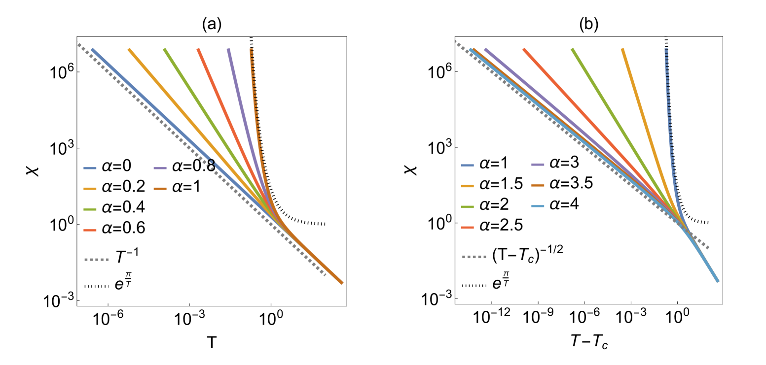
Figure 4: (a) Scaling plot of static spin susceptibility $\chi$ for $\alpha\leq 1$. For $\alpha<1$, $\chi$ exhibits a power-law divergence for $T\ll 1$. The power-law exponent increases with $\alpha$ and diverges in the limit $\alpha\to 1$. For $\alpha=1$, $\chi$ diverges exponentially $\chi\sim e^{\pi/T}$. (b) Scaling plot for $\alpha\geq 1$ as a function of $T-T_{c}$. For $\alpha>1$, $\chi$ exhibits a power-law divergence near $T_{c}$. The exponent decreases with $\alpha$ and converges to $1/2$ for $\alpha>3$.

4 Non-ergodic phase

The response function (13) in real space decays exponentially

$$G(t)=\theta(t)e^{-\frac{t}{\tau}},\quad\tau=\frac{1}{\mu}.$$ (17)

The relaxation time $\tau$ diverges at $T=T_{c}$ with the same critical exponent as that of $\chi$, suggesting the ergodicity breaking. Here, we define and investigate the order parameter in the non-ergodic phase.

First, note that the spherical condition in the form (10) can not be satisfied for any $\mu$ for $T<T_{c}$. As we will see below, the equation needs to be modified for $\mu=0$. For this purpose, it is convenient to write the spin variable as

$$\sigma_{i}(t)=\sigma_{i}^{0}+\delta\sigma_{i}(t),$$ (18)

where $\sigma_{i}^{0}$ denotes the time independent part depending on the initial condition, and $\delta\sigma_{i}(t)$ denotes the fluctuation around it. When $\mu=0$, the EOM (3) reduces to

$$\delta\dot{\sigma}_{i}=\xi_{i}.$$ (19)

Repeating the same analysis as in the previous section, the spherical constraint is now written as

$$1=\frac{1}{N}\sum_{i=1}^{N}\left\langle\left(\sigma_{i}^{0}\right)^{2}\right\rangle+\frac{1}{N}\sum_{i=1}^{N}\left\langle\delta\sigma_{i}^{2}\right\rangle=q+\frac{T}{\pi}\int_{0}^{\infty}d\omega\frac{D(\omega)}{\omega^{2}},$$ (20)

where we have defined the ergodicity breaking parameter as follows:

$$q=\frac{1}{N}\sum_{i=1}^{N}\left\langle\left(\sigma_{i}^{0}\right)^{2}\right\rangle.$$ (21)

Using Eqs. (11) and (20), we get

$$q=1-\frac{T}{T_{c}}.$$ (22)

The order parameter $q$ increases continuously from the transition point $T_{c}$. The scaling behavior of the order parameter does not depend on $\alpha$, as in the case of the original spherical model for ferromagnet [33, 39].

5 Summary and discussions

In this work, we investigated the spherical model driven by the temporally hyperuniform noise whose spectrum for small $\omega$ is written as $D(\omega)\sim\left|\omega\right|^{\alpha}$. For $\alpha>1$, the model undergoes the ergodicity breaking even without spin-spin interactions. In the ergodic phase, we calculated the static spin susceptibility $\chi$ to characterize the criticality near the transition point. The susceptibility $\chi$ exhibits a power-law divergence toward the transition point. The critical exponent takes a non-trivial value that varies depending on $\alpha$. The relaxation time diverges with the same critical exponent as that of $\chi$. In the non-ergodic phase, the order parameter increases continuously from the transition point, where the scaling does not depend on $\alpha$.

A key ingredient of the ergodicity breaking of the current model is the strong anticorrelation of the noise. The spherical model can be considered as a free particle on the $N$-dimensional hypersphere of the radius $\sqrt{N}$. For simplicity, consider a free particle driven by class I hyperuniform noise, $\dot{x}=\xi$, whose noise spectrum for small $\omega$ behaves as $D(\omega)\sim T\omega^{\alpha}$ with $\alpha>1$. In the long-time limit, the mean-squared displacement converges to a finite value $\lim_{t\to\infty}\left\langle(x(t)-x(0))^{2}\right\rangle\propto T$ [41, 19], implying that the particle remains localized within a region with the linear size $O(T^{1/2})$. This complete suppression of diffusion is an alternative definition of class I hyperuniformity in one dimension [1]. The same scenario may also apply to the free particle on the hypersphere: for sufficiently small $T$, the particle cannot explore the entire region on the hypersphere, thereby leading to the ergodicity breaking.

The ergodicity breaking of the current model can also be interpreted as a condensation transition in frequency space to the zero frequency state $\sigma_{i}^{0}$, where the global spherical constraint plays an essential role [42]. A natural and important question is whether similar phenomena occur under alternative global constraints encountered in other fields, such as constraint satisfaction problems [43, 44], theoretical ecology [45], economics, and finance [46].

References

References

- [1] Torquato S 2018 Physics Reports 745 1–95
- [2] Torquato S and Stillinger F H 2003 Phys. Rev. E 68(4) 041113 URL https://link.aps.org/doi/10.1103/PhysRevE.68.041113
- [3] Kim J and Torquato S 2018 Phys. Rev. B 97(5) 054105 URL https://link.aps.org/doi/10.1103/PhysRevB.97.054105
- [4] Oğuz E C, Socolar J E S, Steinhardt P J and Torquato S 2017 Phys. Rev. B 95(5) 054119 URL https://link.aps.org/doi/10.1103/PhysRevB.95.054119
- [5] Koga A, Sakai S, Matsushita Y and Ishimasa T 2024 Phys. Rev. B 110(9) 094208 URL https://link.aps.org/doi/10.1103/PhysRevB.110.094208
- [6] Donev A, Stillinger F H and Torquato S 2005 Phys. Rev. Lett. 95(9) 090604 URL https://link.aps.org/doi/10.1103/PhysRevLett.95.090604
- [7] Hopkins A B, Stillinger F H and Torquato S 2012 Phys. Rev. E 86(2) 021505 URL https://link.aps.org/doi/10.1103/PhysRevE.86.021505
- [8] Ikeda A and Berthier L 2015 Phys. Rev. E 92(1) 012309 URL https://link.aps.org/doi/10.1103/PhysRevE.92.012309
- [9] Hexner D, Liu A J and Nagel S R 2018 Phys. Rev. Lett. 121(11) 115501 URL https://link.aps.org/doi/10.1103/PhysRevLett.121.115501
- [10] Hexner D, Urbani P and Zamponi F 2019 Phys. Rev. Lett. 123(6) 068003 URL https://link.aps.org/doi/10.1103/PhysRevLett.123.068003
- [11] Bolton-Lum V, Dennis R C, Morse P and Corwin E 2024 arXiv preprint arXiv:2404.07492
- [12] Wang Y, Qian Z, Tong H and Tanaka H 2025 Nature Communications 16 1398
- [13] Hexner D and Levine D 2017 Physical review letters 118 020601
- [14] Lei Q L, Ciamarra M P and Ni R 2019 Science advances 5 eaau7423
- [15] Lei Q L and Ni R 2019 Proceedings of the National Academy of Sciences 116 22983–22989
- [16] Kuroda Y and Miyazaki K 2023 Journal of Statistical Mechanics: Theory and Experiment 2023 103203
- [17] Galliano L, Cates M E and Berthier L 2023 Phys. Rev. Lett. 131(4) 047101 URL https://link.aps.org/doi/10.1103/PhysRevLett.131.047101
- [18] Ikeda H 2023 Phys. Rev. E 108(6) 064119 URL https://link.aps.org/doi/10.1103/PhysRevE.108.064119
- [19] Ikeda H 2024 SciPost Phys. 17 103 URL https://scipost.org/10.21468/SciPostPhys.17.4.103
- [20] Maire R and Plati A 2024 The Journal of Chemical Physics 161 054902
- [21] Kuroda Y, Kawasaki T and Miyazaki K 2025 Phys. Rev. Res. 7(1) L012048 URL https://link.aps.org/doi/10.1103/PhysRevResearch.7.L012048
- [22] Ikeda H and Kuroda Y 2024 Phys. Rev. E 110(2) 024140 URL https://link.aps.org/doi/10.1103/PhysRevE.110.024140
- [23] Florescu M, Torquato S and Steinhardt P J 2009 Proceedings of the National Academy of Sciences 106 20658–20663
- [24] Sire C 1993 International Journal of Modern Physics B 7 1551–1567
- [25] Schwartz M, Villain J, Shapir Y and Nattermann T 1993 Phys. Rev. B 48(5) 3095–3099 URL https://link.aps.org/doi/10.1103/PhysRevB.48.3095
- [26] Chandran A and Laumann C R 2017 Phys. Rev. X 7(3) 031061 URL https://link.aps.org/doi/10.1103/PhysRevX.7.031061
- [27] Sakai S, Arita R and Ohtsuki T 2022 Phys. Rev. Res. 4(3) 033241 URL https://link.aps.org/doi/10.1103/PhysRevResearch.4.033241
- [28] Luck J M 1993 Journal of statistical physics 72 417–458
- [29] Crowley P J D, Laumann C R and Gopalakrishnan S 2019 Phys. Rev. B 100(13) 134206 URL https://link.aps.org/doi/10.1103/PhysRevB.100.134206
- [30] Tjhung E and Berthier L 2017 Phys. Rev. E 96(5) 050601 URL https://link.aps.org/doi/10.1103/PhysRevE.96.050601
- [31] Liebchen B and Levis D 2022 Europhysics Letters 139 67001
- [32] Zhang Y and Fodor E 2023 Phys. Rev. Lett. 131(23) 238302 URL https://link.aps.org/doi/10.1103/PhysRevLett.131.238302
- [33] Berlin T H and Kac M 1952 Physical Review 86 821
- [34] Stanley H E 1968 Phys. Rev. 176(2) 718–722 URL https://link.aps.org/doi/10.1103/PhysRev.176.718
- [35] Kirkpatrick T R and Thirumalai D 1987 Phys. Rev. Lett. 58(20) 2091–2094 URL https://link.aps.org/doi/10.1103/PhysRevLett.58.2091
- [36] Crisanti A and Sommers H J 1992 Zeitschrift für Physik B Condensed Matter 87 341–354
- [37] Castellani T and Cavagna A 2005 Journal of Statistical Mechanics: Theory and Experiment 2005 P05012
- [38] Cavagna A 2009 Physics Reports 476 51–124
- [39] Nishimori H and Ortiz G 2010 Elements of phase transitions and critical phenomena (Oup Oxford)
- [40] Henkel M, Hinrichsen H, Lübeck S and Pleimling M 2008 Non-equilibrium phase transitions vol 1 (Springer)
- [41] Eliazar I and Klafter J 2009 Proceedings of the National Academy of Sciences 106 12251–12254
- [42] Crisanti A, Sarracino A and Zannetti M 2019 Phys. Rev. Research 1(2) 023022 URL https://link.aps.org/doi/10.1103/PhysRevResearch.1.023022
- [43] Mezard M and Montanari A 2009 Information, physics, and computation (Oxford University Press)
- [44] Franz S, Parisi G, Sevelev M, Urbani P and Zamponi F 2017 SciPost Physics 2 019
- [45] Altieri A 2022 arXiv preprint arXiv:2208.14956
- [46] Bouchaud J P, Marsili M and Nadal J P 2023 Application of spin glass ideas in social sciences, economics and finance Spin Glass Theory and Far Beyond: Replica Symmetry Breaking After 40 Years (World Scientific) pp 561–579