The Role of the Marketplace Operator in Inducing Competition

Abstract

The steady rise of e-commerce marketplaces underscores the need to study a market structure that captures the key features of this setting. To this end, we consider a price-quantity Stackelberg duopoly in which the leader is the marketplace operator and the follower is an independent seller. The objective of the marketplace operator is to maximize a weighted sum of profit and a term capturing positive customer experience, whereas the independent seller solely seeks to maximize their own profit. Furthermore, the independent seller is required to share a fraction of their revenue with the marketplace operator for the privilege of selling on the platform. We derive the subgame-perfect Nash equilibrium of this game and find that the equilibrium strategies depend on the assumed rationing rule. We then consider practical implications for marketplace operators. Finally, we show that, under intensity rationing, consumer surplus and total welfare in the duopoly marketplace is always at least as high as under an independent seller monopoly, demonstrating that it is socially beneficial for the operator to join the market as a seller.

Keywords: Stackelberg Duopoly, Price-Quantity Duopoly, Marketplace Health, Rationing Rules

JEL Codes: D21, D43, L81

1 Introduction

The rapid growth of e-commerce marketplaces has reshaped the retail landscape, with marketplaces such as Amazon, Walmart, and Target playing a dual role: they serve as intermediaries facilitating transactions for third-party sellers while simultaneously competing as direct sellers. This dual role raises important questions about pricing strategies, market competition, and overall welfare. In particular, what role can the marketplace operator play in promoting competition?

To illustrate why inducing competition is a delicate issue, consider the following ways in which a well-intentioned, but naive, marketplace operator can fail to promote genuine competition. First, if the operator enters the market with a price lower than the independent seller’s break-even price, the seller will not compete. Second, even when the operator raises their price above the independent seller’s break-even price, if they do not have enough inventory to “back up” their offering of the product at that price, the seller will simply wait for them to sell out and then charge a higher price. Third, if the operator sets a price that is too high (above the price the independent seller sets by themselves), this exerts no competitive pressure and the independent seller will simply act as if they are the sole seller. In summary, the presence of a competitor does not necessarily imply true competition when marketplace operators have dual roles. Clearly, inducing competition in such marketplaces is a subtle problem that must be carefully analyzed. We formalize this problem and answer: How can the marketplace operator set their price and inventory to induce competition? When is it beneficial for the marketplace operator to induce competition? What are the implications for consumer surplus and total welfare?

To address these questions, we model a price-quantity Stackelberg duopoly where the first mover is the marketplace operator, who seeks to optimize not only their profit but also customer experience. The second mover is an independent seller, who sells on the marketplace and pays a commission on revenue to the marketplace operator. The strategic interactions between these players give rise to equilibrium behaviors that depend on how demand is rationed between them. In addition to online retailers, our model can more generally be applied to physical marketplaces such as Best Buy, Costco, and supermarkets, which often offer private-label products that compete with name-brand versions on their shelves.

A central result we will show is that it can often be optimal for the marketplace operator to buy inventory that they know they will never sell, for the purpose of inducing the independent seller to set a competitive price. This result demonstrates the important role responsible market operators can play in protecting customers from price hikes by promoting competition.

We also find that the consumer surplus and welfare when the marketplace operator enters the market is always as high as when the independent seller is the only seller. Although in this paper we focus on the interaction between the market operator and a single seller, in reality the marketplace operator is simultaneously participating in multiple copies of this game over a large number of products sold by different sellers. Taking the multiplicity of games into account implies that the marketplace operator can have a significant impact on total welfare by entering the market as a seller.

Outline of paper.

In Section 2, we formally introduce our setting and the rationing rules we consider. In Section 3, we derive the independent seller’s best response function given the price and inventory of the marketplace operator, and we discuss the implications for competition. In Section 4, we characterize the equilibrium of our game. In Section 5, we analyze implications for consumer surplus and welfare. In Section 6, we consider an extension to a form of imperfect substitutability. In Section 7, we conclude.

1.1 Related literature

We draw upon many classical ideas in economics to analyze the modern problem of competition on online retail marketplaces.

Non-simultaneous duopolies.

Early work on duopolies consider simultaneous actions with a single decision variable (either price or quantity). In a Cournot duopoly (Cournot, 1897), sellers $A$ and $B$ simultaneously choose their quantities $q_{A}$ and $q_{B}$ and each face a price $p=f(q_{A}+q_{B})$. In a Bertrand duopoly (Bertrand, 1883), sellers simultaneously choose their prices $p_{A}$ and $p_{B}$, then the lower-priced seller $i\in\{A,B\}$ gets demand $D(p_{i})$ and the other gets zero demand. When $p_{A}=p_{B}$, each seller gets demand $D(p_{i})/2$.

The study of non-simultaneous duopolies began with Stackelberg (1934), who analyzes a sequential version of the Cournot duopoly where one seller is a “leader,” who sets their quantity first and the other seller is a “follower,” who sets their quantity only after observing the leader’s quantity. “Stackelberg” is now generally used to refer to games with a leader and a follower. Whereas Stackelberg games are two-stage games, Maskin and Tirole (1988) consider an infinite-stage game where two sellers take turns choosing prices ad infinitum. They use this model to formalize the phenomenon first presented in Edgeworth (1925) (now called the “Edgeworth cycle”) that there is no pure-strategy equilibrium in the infinite sequential game. Pal (1998) and subsequent work by Nakamura and Inoue (2009) and others study the question of when non-simultaneous duopolies arise naturally between a public and private firm by modeling timing as an endogenous decision. In our paper, we analyze a sequential game with two decision variables — price and quantity.

Capacity constraints and rationing rules.

When price and quantity are both decision variables, we are required to think carefully about how demand is split between sellers. In other words, to analyze games in which players are only able to sell up to an exogenous or endogenously chosen inventory level (i.e., capacity-constrained games), we must specify rationing rules. Shubik (1959) and Levitan and Shubik (1978) propose and solve the Bertrand-Edgeworth game, which is the capacity-constrained price competition game. Kreps and Scheinkman (1983) consider a two-stage duopoly where both firms choose their inventory in the first stage then set their price in the second stage. They make the intensity rationing assumption (see their Equation 2) and show that under certain conditions, the equilibrium of the two-stage game is the same as in the Cournot duopoly. Later work by Davidson and Deneckere (1986) shows that this result relies crucially on the intensity rationing assumption and does not hold under other rationing assumptions, in particular, proportional rationing. At the proportional rationing equilibrium, firms choose larger capacities and receive less profit than under intensity rationing. With this in mind we consider both intensity and proportional rationing rules in this paper. See Section 14.2 of Rasmusen (1989) or Section 5.3.1 of Tirole (1988) for an overview of rationing rules. Closely related to our work is Boyer and Moreaux (1987), who study sequential duopolies with both price and quantity as decision variables, and Boyer and Moreaux (1989) and Yousefimanesh et al. (2023), which analyze a similar setting but with imperfectly substitutable goods.

Mixed oligopolies.

In a mixed oligopoly, welfare-maximizing public firm(s) compete with profit-maximizing private firm(s) (Cremer et al., 1989; De Fraja and Delbono, 1990). Our model represents an intermediate between a standard private-private duopoly and a mixed public-private duopoly. The independent seller is a standard private firm, but the marketplace operator can be viewed as somewhere between private and public: “private” because they are utility-maximizing rather than welfare-maximizing but close to “public” because their utility function internalizes consumer benefit (via the $k$ term, as will be described in Section 2).

Marketplaces.

Whereas the aforementioned related works are all from classical economics literature, the applied motivation of our work most closely relates to recent work that models game dynamics on online marketplaces. There is a line of work that models compatibility between buyers and sellers via networks (Birge et al., 2021; Banerjee et al., 2017; D’Amico-Wong et al., 2024; Eden et al., 2023), which also relates more broadly to two-sided markets and platform economics (Caillaud and Jullien, 2003; Armstrong, 2006; Rochet and Tirole, 2003). Unlike these works, we model the marketplace operator itself as a seller, similar to Pabari et al. (2025). They analyze the equilibrium of the simultaneous price-competition game and consider the problem of setting the referral fee. Also related is Shopova (2023), who studies the effect of a marketplace operator introducing a lower quality private-label product in a price duopoly setting.

Despite the widespread dominance of e-commerce marketplaces and platform-driven competition, the strategic interaction between marketplace operators and independent sellers has not been well studied. Our work directly addresses this need by developing an asymmetric price-quantity duopoly model that captures the core dynamics of platform competition. Unlike prior work, we explicitly analyze multiple rationing rules to reflect a range of real-world scenarios, providing a framework that is not only theoretically rigorous but also practically relevant for designing pricing and inventory strategies in marketplaces.

2 Setting

We now describe the game we study. Our game has two players: a marketplace operator ($\mathtt{MO}$) and an independent seller ($\mathtt{IS}$). We assume the two players sell identical products, although we will consider an extension to imperfect substitutability in Section 6. Despite selling the same product, $\mathtt{MO}$ and $\mathtt{IS}$ can acquire or produce the product at different costs, specifically $c_{\mathtt{MO}}\geq 0$ and $c_{\mathtt{IS}}\geq 0$ per unit respectively. $\mathtt{MO}$ operates the market in which the players sell their products and so $\mathtt{IS}$ pays $\mathtt{MO}$ a fraction $\alpha\in[0,1]$ of their revenue per unit as a referral fee, and $\mathtt{MO}$ realizes benefit $k\geq 0$ for every unit sold to account for the customers’ positive experience, which contributes to the health of the marketplace. The number of units each player can sell is the minimum of their inventory and their demand, and any unsold units have zero value. Players are allowed to buy and sell fractional units. A formal definition of the game, including actions and order of play, can be found in Game 2.

There are two primary reasons we model the game as occurring sequentially in Game 2. The first is an operational limitation: larger often means less agile. Large platforms with complex interlocking operations must commit to decisions well in advance in order for business to run smoothly. Third-party sellers on the other hand generally have fewer moving parts to handle and can thus be more reactive. Additionally, marketplaces often offer promotions, which require pre-determining pricing and the necessary inventory. The second justification is that, as the platform operator, $\mathtt{MO}$ has control of the information flow and thus has commitment power. As soon as $\mathtt{MO}$ has made their decisions, they can announce it to $\mathtt{IS}$, and $\mathtt{IS}$ then selects their own strategy with knowledge of what strategy $\mathtt{MO}$ has already committed to.

2.1 Demand function

Before we can study the game, we first need to specify each player’s demand function, which can be thought of in terms of “original” and “residual” demand functions. The player $j\in\{\mathtt{MO},\mathtt{IS}\}$ that sets the lower price faces the original demand function $Q(p_{j})$ and the other seller $i$ faces the residual demand function $R(p_{i};q_{j},p_{j})$. If prices are equal, the tie is broken in favor of $\mathtt{IS}$. The two players’ demand functions are thus given by

$$D_{\mathtt{IS}}(p_{\mathtt{IS}};q_{\mathtt{MO}},p_{\mathtt{MO}})=\begin{cases}Q(p_{\mathtt{IS}})&\text{if }p_{\mathtt{IS}}\leq p_{\mathtt{MO}}\\ R(p_{\mathtt{IS}};q_{\mathtt{MO}},p_{\mathtt{MO}})&\text{if }p_{\mathtt{IS}}>p_{\mathtt{MO}},\end{cases}$$

$$D_{\mathtt{MO}}(p_{\mathtt{MO}};q_{\mathtt{IS}},p_{\mathtt{IS}})=\begin{cases}R(p_{\mathtt{MO}};q_{\mathtt{IS}},p_{\mathtt{IS}})&\text{if }p_{\mathtt{IS}}\leq p_{\mathtt{MO}}\\ Q(p_{\mathtt{MO}})&\text{if }p_{\mathtt{IS}}>p_{\mathtt{MO}}.\end{cases}$$

Original demand function. For mathematical concreteness, we assume a linear demand function with unit slope and intercept $\theta\geq 0$. $\theta$ corresponds to the maximum willingness to pay of any customer and is also the number of units that would be demanded if the price were zero.

Assumption 1 (Linear demand).

The quantity demanded at price $p$ is

$$Q(p)=\begin{cases}\theta-p&\text{for $0\leq p\leq\theta$}\\ 0&\text{for $p>\theta$}.\end{cases}$$

Rationing rules and residual demand functions. The residual demand function is determined by a rationing rule that determines which customers are able to buy at the lower price and which remain for the higher-priced seller. There exists a wide range of reasonable rationing rules and associated residual demand functions, and they have varying degrees of favorability for the higher-price seller (Rasmusen, 1989). Before diving into specific rationing rules, we first formalize the minimal assumptions that any residual demand function should satisfy.

Move the residual functions assumptions to the appendix as they are all very intuitive and don’t add much to the discussion? If you do so, I would remove the sentences ”Before getting into rationing rules.. .” and ”We now introduce…” and replace ”We now introduce..” simply by ”We discuss three notable examples of rationing rules, starting with the least favorable to the high-priced seller.” .. Then, at the end of the list of three, also replace ”We provide an extended discussion..” with ”We formalize minimal assumptions that any residual demand function should satisfy and provide an extended discussion of rationing rules in Appendix A.”

Assumption 2.

The residual demand function $R(p_{i};q_{j},p_{j})$, where $p_{i}$ denotes the price of the higher-priced seller and $q_{j}$ and $p_{j}$ are the inventory and price of the lower-priced seller, satisfies

1. $R(p_{i};q_{j},p_{j})\leq Q(p_{i})$ for all $p_{i}\in[0,\theta]$ — the residual demand cannot exceed the original demand at the same price.

2. $R(p_{i};q_{j},p_{j})\geq 0$ for all $p_{i}\in[0,\theta]$ — the residual demand cannot be negative.

3. $\frac{\partial}{\partial p_{i}}R(p_{i};q_{j},p_{j})\leq 0$ — as the higher-priced seller increases their price, their demand decreases or does not change.

4. $\frac{\partial}{\partial q_{j}}R(p_{i};q_{j},p_{j})\leq 0$ — if the lower-priced seller increases their inventory, this decreases or does not change the demand left over for the higher-priced seller.

To avoid clutter we will sometimes omit the dependence of $R$ on $q_{j}$ and $p_{j}$ and simply write $R(p_{i})$.

We now introduce some notable examples of residual demand functions that we will analyze later. Specifically, we consider residual demand functions induced by three rationing rules (and their generalizations), starting with the rule that is least favorable to the higher-priced seller.two rationing rules and their generalizations.

1. Intensity rationing (also known as efficient rationing): Assuming that the highest-valuation customers buy first (i.e., at the lower price) yields the residual demand function

   $$R(p_{i})=Q(p_{i})-q_{j}.$$

   This is a member of the class of subtractive residual demand functions, which are functions that can be represented as

   $$R(p_{i})=Q(p_{i})-f(q_{j})$$

   for some $f:[0,\theta]\to[0,\theta]$ that is an increasing function of $q_{j}$ satisfying $f(0)=0$ and $f(q)\leq q$ for all $q\in[0,\theta]$.

2. Proportional rationing (also known as Beckmann rationing; see Davidson and Deneckere (1986)): Suppose that every customer has the same probability $\rho$ of being assigned to the lower-priced seller, where $\rho$ is such that in expectation the demand that the lower-price seller faces at their price $p_{i}$ is exactly equal to their supply $q_{i}$. This yields

   $$R(p_{i})=Q(p_{i})\left(1-\frac{q_{j}}{Q(p_{j})}\right).$$

   This is a member of the class of multiplicative demand functions, which are functions that can be represented as

   $$R(p_{i})=Q(p_{i})g(q_{j})$$

   where $g:[0,\theta]\to[0,1]$ is a decreasing function of $q_{j}$ satisfying $g(0)=1$. $g$ can also depend on $p_{j}$.

3. Inverse intensity rationing (also known as inefficient rationing): Assuming that the lowest-valuation customers buy first yields the residual demand function

   $$R(p_{i})=\min\big{(}Q(p_{i}),\theta-q_{j}\big{)}$$

   This is a member of the class of truncated demand functions, which are functions that can be represented as

   $$R(p_{i})=\min\big{(}Q(p_{i}),\theta-h(q_{j})\big{)}$$

   where $h:[0,\theta]\to[0,\theta]$ is an increasing function of $q_{j}$ satisfying $h(0)=0$.

Figure 1 visualizes the residual demand functions induced by each of the named rationing rules. We provide an extended discussion of rationing rules in Appendix A.

(a) Intensity

(b) Proportional

Figure 1: Visualization of $R(p_{\mathtt{IS}})$ for $\theta=4$, $q_{\mathtt{MO}}=1$, and $p_{\mathtt{MO}}=2$ under three rationing rules: intensity, proportional, and inverse intensity.intensity rationing and proportional rationing.

2.2 Preliminaries

We now introduce some definitions that will be used to characterize the equilibrium. Recall that $\mathtt{IS}$’s utility (i.e., net profit) from selling one unit of the good at price $p$ after paying the referral fee $\alpha$ is $(1-\alpha)p-c_{\mathtt{IS}}$.

Definition 1.

$\mathtt{IS}$’s break-even price $p_{0}$ is the price at which they get zero utility from selling the good:

$$p_{0}=\frac{c_{\mathtt{IS}}}{1-\alpha}$$

We assume that given the choice between selling a positive quantity at $p_{0}$ vs. not selling at all, $\mathtt{IS}$ will choose to sell at $p_{0}$.

Definition 2.

$\mathtt{IS}$’s optimal sole-seller price $p^{\star}_{\mathtt{IS}}$ is the price the independent seller would set when the marketplace operator is not a seller ($q_{\mathtt{MO}}=0$):

$$p^{\star}_{\mathtt{IS}} =\arg\max_{p}((1-\alpha)p-c_{\mathtt{IS}})Q(p)$$

$$=\begin{cases}\infty&\text{if }p_{0}>\theta\\ \frac{1}{2}(p_{0}+\theta)&\text{otherwise},\end{cases}$$

where $\infty$ can be interpreted to be any price that is above $\theta$ or, equivalently, any price $p$ at which $Q(p)=0$.

We see in the previous displayed equation that if $c_{\mathtt{IS}}$ and $\alpha$ are so high that $p_{0}>\theta$, the independent seller will not sell. This results in a simple, near trivial, solution of the game, which we describe in the following proposition.

Proposition 1.

Whenever $p_{0}>\theta$, the equilibrium solution of Game 2 is $\mathtt{IS}$ does not sell ($q_{\mathtt{IS}}=0$) and $\mathtt{MO}$ sets price $p^{\star}_{\mathtt{MO}}$ and quantity $Q(p^{\star}_{\mathtt{MO}})$, where

$$p^{\star}_{\mathtt{MO}} =\arg\max_{p}(p+k-c_{\mathtt{MO}})Q(p)$$

$$=\begin{cases}\infty&\text{if }c_{\mathtt{MO}}>\theta+k\\ \frac{1}{2}(c_{\mathtt{MO}}-k+\theta)&\text{otherwise.}\end{cases}$$

Since the $p_{0}>\theta$ does not generally occur in the real world (this would mean, e.g., that an independent seller’s manufacturing cost is close to customers’ maximum willingness to pay) and is also uninteresting, we will focus on analyzing the $p_{0}\leq\theta$ case.

By entering the market, $\mathtt{MO}$ can cause $\mathtt{IS}$ to deviate from their sole-seller price. We now provide some terminology to refer to specific phenomena that can arise.

Definition 3.

We say that $\mathtt{IS}$ has been de-monopolized if they set $p_{\mathtt{IS}}<p^{\star}_{\mathtt{IS}}$, i.e., they set a price strictly lower than their optimal sole-seller price.

Definition 4.

When $\mathtt{MO}$’s price is higher than $\mathtt{IS}$’s optimal sole-seller price ($p_{\mathtt{MO}}\geq p^{\star}_{\mathtt{IS}}$), we say that $\mathtt{IS}$ passively competes if they choose $p_{\mathtt{IS}}=p^{\star}_{\mathtt{IS}}\leq p_{\mathtt{MO}}$.

Definition 5.

We say that $\mathtt{IS}$ is competing if $p_{\mathtt{IS}}\leq p_{\mathtt{MO}}$ and we describe any $p_{\mathtt{IS}}\leq p_{\mathtt{MO}}$ as a “competitive price.”

We make some remarks about the above definitions. First, note that when $\mathtt{IS}$ “passively competes,” they are not setting a lower price than they would have without $\mathtt{MO}$ as a seller, but they are still “competing” because they are setting a price lower than or equal to $\mathtt{MO}$’s price. Second, note that competing is implied by passively competing but competing is not required to be de-monopolized (we will see an example later where $\mathtt{IS}$ is de-monopolized even when they are not competing). Third, note that being de-monopolized and passively competing are mutually exclusive.

2.3 Solution concept

The natural solution concept for sequential games, including ours, is the subgame-perfect Nash equilibrium, which is defined as follows.

Definition 6.

Let $a=(p_{\mathtt{MO}},q_{\mathtt{MO}})$ be $\mathtt{MO}$’s action and let $b(a)=(p_{\mathtt{IS}}(a),q_{\mathtt{IS}}(a))$ be $\mathtt{IS}$’s action when $\mathtt{MO}$ chose action $a$. A strategy profile $(a^{*},b^{*}(a))$ constitutes a subgame-perfect Nash equilibrium if and only if for every $\mathtt{MO}$ action $a$, $\mathtt{IS}$’s strategy $b^{*}(a)$ satisfies

$$b^{*}(a)=\arg\max_{b}u_{\mathtt{IS}}(a,b),$$

and $\mathtt{MO}$’s strategy $a^{*}$ satisfies

$$a^{*}=\arg\max_{a}u_{\mathtt{MO}}(a,b^{*}(a)).$$

Definition 6 means that $\mathtt{IS}$ plays its best response $b^{*}(a)$ to $\mathtt{MO}$’s action $a$ while $\mathtt{MO}$ chooses $a^{*}$ to maximize their own payoff given the best-response function $b^{*}(a)$.

3 Independent Seller’s Best Response

The first step to determining the equilibrium is to derive the independent seller’s best response. We summarize the independent seller’s best response as a function of $p_{\mathtt{MO}}$ and $q_{\mathtt{MO}}$ via four propositions. We also convey the results from these propositions visually in Figure 2 to help with interpretation. All omitted proofs can be found in Appendix B.

Our first proposition, which is similar to Proposition 1 of Yousefimanesh et al. (2023), formalizes the intuition that the independent seller should sell as much as they can at their chosen price, so they should set their quantity to exactly meet their demand. This follows from the fact that, unlike the marketplace operator, $\mathtt{IS}$ only benefits from directly selling the product. Although we state the result in a way that implies the maximizing $q_{\mathtt{IS}}$ can be non-unique, we remark that the only case in which there is no unique optimal $q_{\mathtt{IS}}$ given $p_{\mathtt{IS}}$ is if $p_{\mathtt{IS}}=p_{0}$. In that case, any $q_{\mathtt{IS}}\leq D_{\mathtt{IS}}(p_{\mathtt{IS}};q_{\mathtt{MO}},p_{\mathtt{MO}})$ is optimal. In all other cases, $q_{\mathtt{IS}}=D_{\mathtt{IS}}(p_{\mathtt{IS}};q_{\mathtt{MO}},p_{\mathtt{MO}})$ is the unique optimal quantity.

Proposition 2 ($\mathtt{IS}$ meets demand).

Given fixed $p_{\mathtt{IS}}$, $q_{\mathtt{MO}}$, and $p_{\mathtt{MO}}$, if there exists $q_{\mathtt{IS}}$ such that $u_{\mathtt{IS}}(p_{\mathtt{MO}},q_{\mathtt{MO}},p_{\mathtt{IS}},q_{\mathtt{IS}})\geq 0$ (which happens if and only if $p_{\mathtt{IS}}\geq p_{0}$), then we must have

$$D_{\mathtt{IS}}(p_{\mathtt{IS}};q_{\mathtt{MO}},p_{\mathtt{MO}})\in\arg\max_{q_{\mathtt{IS}}\geq 0}u_{\mathtt{IS}}(p_{\mathtt{MO}},q_{\mathtt{MO}},p_{\mathtt{IS}},q_{\mathtt{IS}}),$$

i.e., it is utility-maximizing for $\mathtt{IS}$ to set $q_{\mathtt{IS}}$ equal to their demand.

Proof.

First consider the case where $\mathtt{IS}$ sets $p_{\mathtt{IS}}=\infty$, effectively abstaining from selling. Then the optimal inventory is $q_{\mathtt{IS}}=D_{\mathtt{IS}}(p_{\mathtt{IS}};q_{\mathtt{MO}},p_{\mathtt{MO}})=0$ because purchasing any positive amount of inventory incurs positive cost but yields no benefit since there is no demand at an infinite price. Now consider the case where $p_{\mathtt{IS}}\in(p_{0},\infty)$. It is sub-optimal to set $q_{\mathtt{IS}}<D_{\mathtt{IS}}(p_{\mathtt{IS}};q_{\mathtt{MO}},p_{\mathtt{MO}})$ because the net utility $\mathtt{IS}$ gets from selling each unit is constant, so they could have gotten more utility by selling as many units as they are able to at price $p_{\mathtt{IS}}$. It is also sub-optimal to set $q_{\mathtt{IS}}>D_{\mathtt{IS}}(p_{\mathtt{IS}};q_{\mathtt{MO}},p_{\mathtt{MO}})$ because $\mathtt{IS}$ incurs a cost for acquiring the excess units but these units yield no positive utility because they are not sold. Finally, consider the case where $p_{\mathtt{IS}}=p_{0}$. In this case, the seller gets zero net utility per sale, so any $q_{\mathtt{IS}}\in[0,D_{\mathtt{IS}}(p_{\mathtt{IS}};q_{\mathtt{MO}},p_{\mathtt{MO}}))$ is optimal. ∎

Given Proposition 2, we can focus on deriving $\mathtt{IS}$’s best response in terms of their price $p_{\mathtt{IS}}$ with the assumption that they will correspondingly set their inventory to $q_{\mathtt{IS}}=D_{\mathtt{IS}}(p_{\mathtt{IS}};q_{\mathtt{MO}},p_{\mathtt{MO}})$. We can thus remove the dependence of $\mathtt{IS}$’s utility on $q_{\mathtt{IS}}$ by plugging in the best response condition, like so:

$$u_{\mathtt{IS}}(p_{\mathtt{IS}},p_{\mathtt{MO}},q_{\mathtt{MO}})=[(1-\alpha)p_{\mathtt{IS}}-c_{\mathtt{IS}}]D_{\mathtt{IS}}(p_{\mathtt{IS}};q_{\mathtt{MO}},p_{\mathtt{MO}}).$$ (3)

We additionally adopt the convention that $\mathtt{IS}$ sets $p_{\mathtt{IS}}=\infty$ when they wish to abstain (by setting $q_{\mathtt{IS}}=0$). Having established that $\mathtt{IS}$’s decision reduces to choosing a value of $p_{\mathtt{IS}}$, we now describe the strategies $\mathtt{IS}$ can choose from.

We assume that when $\mathtt{IS}$ is indifferent between competing and not competing, they choose to compete. As the next three propositions will show, which of the above three $\mathtt{IS}$ strategies is optimal depends on the price and quantity chosen by $\mathtt{MO}$. The first of these propositions describes the independent seller’s optimal strategy in the straightforward case where $\mathtt{MO}$ has set a “noncompetitive” (too large) price. The result is intuitive: $p^{\star}_{\mathtt{IS}}$ is the price that $\mathtt{IS}$ would set if the marketplace operator were not a seller, and when the operator does not apply any competitive pressure by setting a lower price, there is no reason for $\mathtt{IS}$ to not set their price to be $p^{\star}_{\mathtt{IS}}$.

Proposition 3 (Large $p_{\mathtt{MO}}$ best response).

Whenever $p_{\mathtt{MO}}\geq p^{\star}_{\mathtt{IS}}$ ($\mathtt{MO}$’s price is higher than $\mathtt{IS}$’s optimal sole-seller price), $\mathtt{IS}$ passively competes by setting $p_{\mathtt{IS}}=p^{\star}_{\mathtt{IS}}$.

In the next proposition, we will consider the more interesting case where $p_{\mathtt{MO}}$ is at an intermediate level ($p_{\mathtt{MO}}\in[p_{0},p^{\star}_{\mathtt{IS}})$), and $\mathtt{MO}$’s inventory level $q_{\mathtt{MO}}$ determines what strategy $\mathtt{IS}$ will take. In other words, $\mathtt{IS}$ must determine if it is worth it to wait it out or if, by the time $\mathtt{MO}$ sells out, there will be so little demand left that it would be better for $\mathtt{IS}$ to compete. This is because whenever $p_{\mathtt{MO}}\geq p_{0}$, the independent seller will never abstain because positive utility is achievable (or in the case of $p_{\mathtt{MO}}=p_{0}$, non-negative utility is achievable, but as described before we assume that $\mathtt{IS}$ is willing to sell at price $p_{0}$). Thus, we simply have to determine whether $\mathtt{IS}$ competes or waits. The following proposition describes the critical $q_{\mathtt{MO}}$ threshold that determines which $\mathtt{IS}$ strategy is optimal. This is obtained by first determining the optimal price that $\mathtt{IS}$ should set when they compete ($p_{\mathtt{MO}}$) and when they wait ($p_{\mathtt{IS}}^{W}$), then comparing the corresponding utilities and choosing the price that achieves the higher utility. The critical threshold $q^{\dagger}(p_{\mathtt{MO}})$ is simply the value of $q_{\mathtt{MO}}$ below which competing yields higher utility and above which waiting yields higher utility. For a function $v:{\mathbb{R}}\to{\mathbb{R}}$, let $v^{-1}:{\mathbb{R}}\to{\mathbb{R}}$ denote its inverse function.

Proposition 4 (Intermediate $p_{\mathtt{MO}}$ best response).

Let $p_{\mathtt{MO}}\in[p_{0},p^{\star}_{\mathtt{IS}})$. The independent seller’s response depends on $\mathtt{MO}$’s inventory, relative to a threshold $q^{\dagger}(p_{\mathtt{MO}})$: if $q_{\mathtt{MO}}\geq q^{\dagger}(p_{\mathtt{MO}})$, the independent seller competes by setting $p_{\mathtt{IS}}=p_{\mathtt{MO}}$; otherwise they wait it out by setting $p_{\mathtt{IS}}=p^{W}_{\mathtt{IS}}$. The threshold function $q^{\dagger}(p_{\mathtt{MO}})$ and wait it out price $p^{W}_{\mathtt{IS}}$ take different forms depending on the residual demand function:

1. For a subtractive residual demand function,

   $$q^{\dagger}(p_{\mathtt{MO}})=f^{-1}\left(\theta-p_{0}-2\sqrt{(p_{\mathtt{MO}}-p_{0})(\theta-p_{\mathtt{MO}})}\right)\qquad\text{and}\qquad p_{\mathtt{IS}}^{W}:=p^{\star}_{\mathtt{IS}}-\frac{f(q_{\mathtt{MO}})}{2}.$$

2. For a multiplicative residual demand function,

   $$q^{\dagger}(p_{\mathtt{MO}})=g^{-1}\left(\frac{(p_{\mathtt{MO}}-p_{0})(\theta-p_{\mathtt{MO}})}{(p^{\star}_{\mathtt{IS}}-p_{0})(\theta-p^{\star}_{\mathtt{IS}})}\right)\qquad\text{and}\qquad p_{\mathtt{IS}}^{W}:=p^{\star}_{\mathtt{IS}}.$$

3. For a truncated residual demand function,

   $$q^{\dagger}(p_{\mathtt{MO}})=h^{-1}(2p^{\star}_{\mathtt{IS}}-p_{\mathtt{MO}})\qquad\text{and}\qquad p_{\mathtt{IS}}^{W}:=\max(p^{\star}_{\mathtt{IS}},h(q_{\mathtt{MO}})).$$

Finally, we consider the case where $\mathtt{MO}$ has set a very low price ($p_{\mathtt{MO}}\leq p_{0}$). Much like Proposition 4, the following proposition determines the independent seller’s best response by comparing $q_{\mathtt{MO}}$ to a critical threshold. The difference in this case is that the strategies $\mathtt{IS}$ is choosing between are to wait or to abstain; competing is no longer a viable option because, by definition of $p_{0}$, $\mathtt{IS}$ is not able to make a profit if they set a price below $p_{\mathtt{MO}}<p_{0}$.

Proposition 5 (Small $p_{\mathtt{MO}}$ best response).

If $p_{\mathtt{MO}}<p_{0}$, the independent seller’s response depends on $\mathtt{MO}$’s inventory, relative to a threshold $q^{\ddagger}(p_{\mathtt{MO}})$: the independent seller abstains by setting $p_{\mathtt{IS}}=\infty$ if $q_{\mathtt{MO}}\geq q^{\ddagger}(p_{\mathtt{MO}})$ and otherwise sets the wait it out price $p_{\mathtt{IS}}^{W}$ described in Proposition 4. The value of the threshold $q^{\ddagger}$ depends on the residual demand function:

1. For a subtractive residual demand function,

   $$q^{\ddagger}(p_{\mathtt{MO}})=f^{-1}(\theta-p_{0})$$

2. For a multiplicative residual demand function,

   $$q^{\ddagger}(p_{\mathtt{MO}})=g^{-1}(0;p_{\mathtt{MO}}),$$

   where we write $g^{-1}(~\cdot~;p_{\mathtt{MO}})$ to emphasize that $g$ can depend on $p_{\mathtt{MO}}$.

3. For a truncated residual demand function,

   $$q^{\ddagger}(p_{\mathtt{MO}})=\theta$$

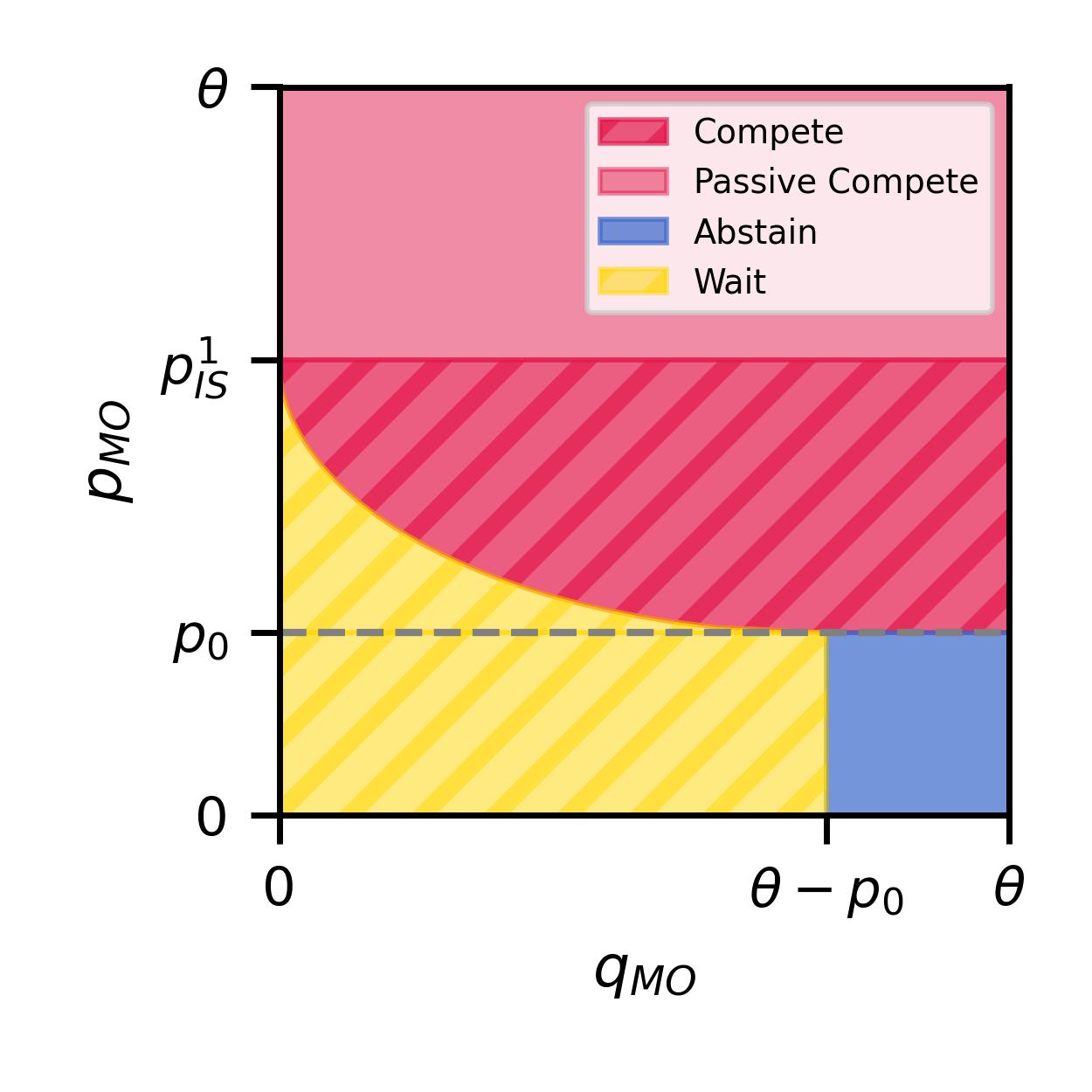
(a) Intensity

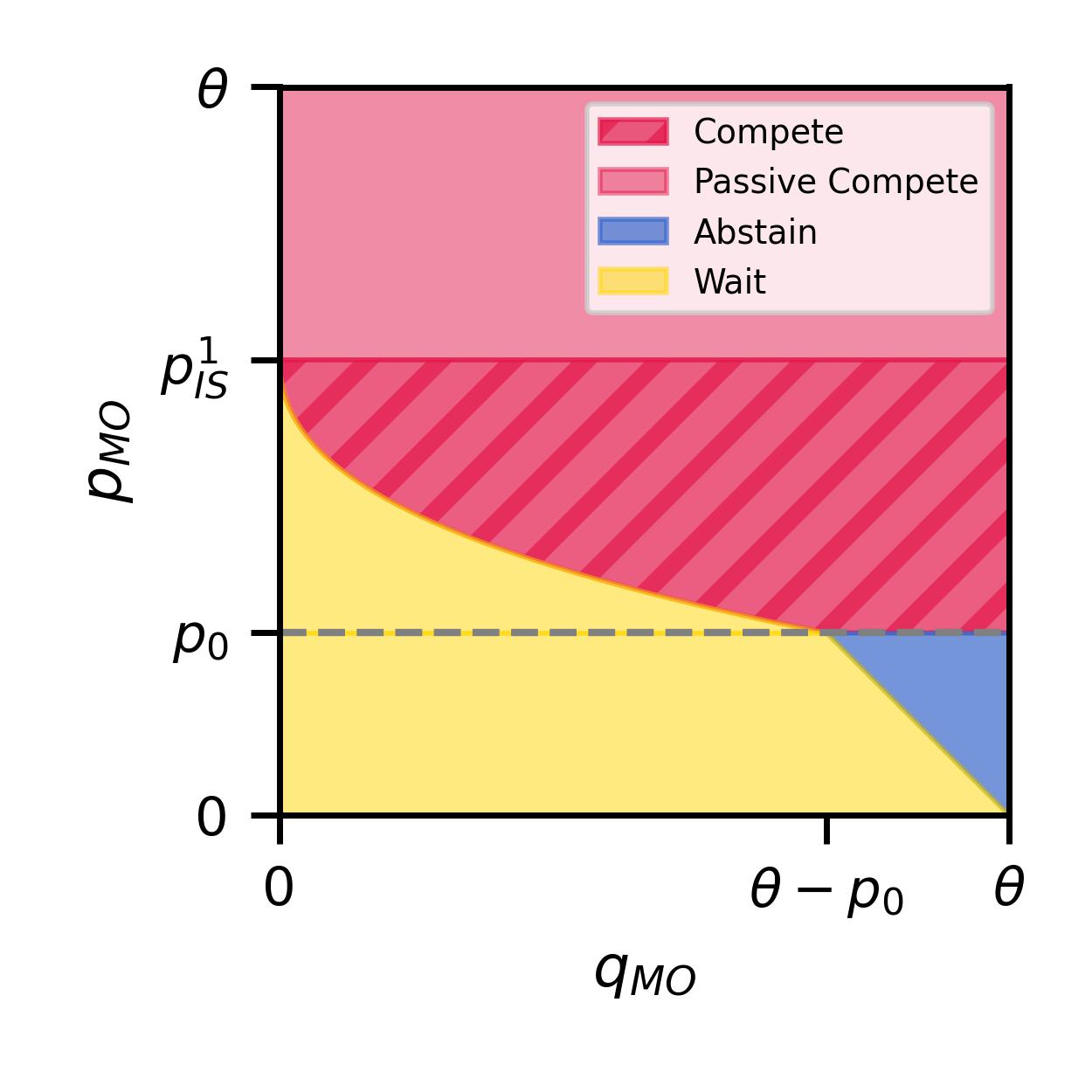
(b) Proportional

Figure 2: Visualization of $\mathtt{IS}$’s best response to different $q_{\mathtt{MO}}$ (x-axis) and $p_{\mathtt{MO}}$ (y-axis) combinations for intensity rationing, proportional rationing, and inverse intensity rationingintensity rationing and proportional rationing. Stripes are used to denote regions where $\mathtt{IS}$ is de-monopolized. Game parameters are set to $\theta=10$, $c_{\mathtt{IS}}=2$, and $\alpha=0.2$ (the value of $c_{\mathtt{MO}}$ does not affect $\mathtt{IS}$’s best response function).

Figure 2 and Table 1 instantiate the results of Propositions 3-5 for intensity rationing and proportional rationing. Figure 2 visualizes the $(p_{\mathtt{MO}},q_{\mathtt{MO}})$ regions where each $\mathtt{IS}$ strategy is optimal and Table 1 summarizes the key quantities and prices that characterize $\mathtt{IS}$’s optimal strategy. The line between the yellow and red regions in Figure 2 is traced out by the threshold function $q^{\dagger}(p_{\mathtt{MO}})$ and the line between the yellow and blue regions is traced out by $q^{\ddagger}(p_{\mathtt{MO}})$.

Figure 2 highlights the large extent to which $\mathtt{IS}$’s best response is dependent on the assumed rationing rule. For example, there are $(p_{\mathtt{MO}},q_{\mathtt{MO}})$ combination that induce compete (are in red region) under intensity rationing but induce wait (are in yellow region) under proportional or inverse intensity rationing. For perfect substitutes, intensity rationing and inverse intensity rationing mark the two ends of the spectrum of possible residual demand functions. The diagrams in Figure 2 make obvious that (1) any $(p_{\mathtt{MO}},q_{\mathtt{MO}})$ that induces wait under intensity rationing will induce wait under any other rationing rule for perfect substitutes and (2) any $(p_{\mathtt{MO}},q_{\mathtt{MO}})$ that induces compete under inverse intensity rationing will induce compete under any other rationing rule for perfect substitutes.Figure 2 illustrates how $\mathtt{IS}$’s best response can change depending on the assumed rationing rule. For example, there are $(p_{\mathtt{MO}},q_{\mathtt{MO}})$ combinations that induce compete (red region) under intensity rationing but induce wait (yellow region) under proportional rationing. There are also $(p_{\mathtt{MO}},q_{\mathtt{MO}})$ combinations that induce abstain (blue region) under intensity rationing but induce wait (yellow region) under proportional rationing.

Table 1: Summary of key values for determining the independent seller’s best response for intensity rationing, proportional rationing, and inverse intensity rationing.intensity rationing and proportional rationing.

	Intensity	Proportional
Compete threshold for $p_{\mathtt{MO}}\in[p_{0},p^{\star}_{\mathtt{IS}})$   $\boxed{q^{\dagger}(p_{\mathtt{MO}})}$	$\theta-p_{0}-2\sqrt{(p_{\mathtt{MO}}-p_{0})(\theta-p_{\mathtt{MO}})}$	$Q(p_{\mathtt{MO}})\left(1-\frac{(p_{\mathtt{MO}}-p_{0})(\theta-p_{\mathtt{MO}})}{(p^{\star}_{\mathtt{IS}}-p_{0})(\theta-p^{\star}_{\mathtt{IS}})}\right)$
Abstain threshold for $p_{\mathtt{MO}}<p_{0}$  $\boxed{q^{\ddagger}(p_{\mathtt{MO}})}$	$\theta-p_{0}$	$Q(p_{\mathtt{MO}})$
$\mathtt{IS}$ price when waiting   $\boxed{p_{\mathtt{IS}}^{W}}$	$p^{\star}_{\mathtt{IS}}-\frac{q_{\mathtt{MO}}}{2}$	$p^{\star}_{\mathtt{IS}}$

3.1 Implications for competition

To provide guidance to marketplace operators who are considering entering their marketplace as a seller for the purpose of promoting competition, we now interpret the independent seller’s best response in the language of competition from Definitions 3-5. We make the following observations.

$p_{\mathtt{MO}}\geq p^{\star}_{\mathtt{IS}}\Rightarrow$ no de-monopolization. The marketplace operator cannot de-monopolize the independent seller if they set a price higher that the independent seller’s sole-seller price. In such instances, the independent seller passively competes by setting the same price as they would have without the marketplace operator (Proposition 3).

$p_{\mathtt{MO}}\leq p_{0}\Rightarrow\mathtt{IS}$ does not compete. Although the previous observation says that a marketplace operator seeking to promote competition should not set their price too high, they also cannot set their price too low: if the marketplace operator sets a price below the independent seller’s break-even price, the independent seller will not compete and will instead either abstain or wait (Proposition 5).

For any rationing rule, $p_{\mathtt{MO}}<p^{\star}_{\mathtt{IS}}$ and compete $\Rightarrow$ de-monopolized. This is tautological but we nonetheless write it for completeness. If the marketplace operator sets a price lower than the independent seller’s sole-seller price and the independent seller competes by setting a price equal to or lower than the marketplace operator’s, then they must be setting a price lower than than their sole-seller price. Under proportional rationing (or any multiplicative residual demand function), and inverse intensity rationing (or any truncated residual demand function)this is an if and only if ($\Leftrightarrow$) because $\mathtt{IS}$’s wait it out price is at least as high as the sole seller price for those rationing rulesequal to the sole seller price under that rationing rule (Proposition 4). The same is not true under intensity rationing, as we we now describe.

For intensity rationing, wait $\Rightarrow$ de-monopolized . Under intensity rationing or any subtractive residual demand function, if the independent seller waits, they will set a price lower than their sole-seller price, i.e., they are de-monopolized. This is worth emphasizing — the independent seller can be de-monopolized even when they are do not choose to compete. This is because under intensity rationing, the residual demand function is simply the original demand function shifted downwards, so when $\mathtt{IS}$ performs their optimization using this downshifted demand function, the optimizing price is lower compared to the original demand function (Proposition 4).

For intensity rationing, $q_{\mathtt{MO}}\uparrow\hskip 2.84526pt\Rightarrow$ “more” de-monopolization when $p_{\mathtt{MO}}\in[p_{0},p^{\star}_{\mathtt{IS}})$. Under intensity rationing (or any subtractive residual demand function), setting $p_{\mathtt{MO}}\in[p_{0},p^{\star}_{\mathtt{IS}})$ and any $q_{\mathtt{MO}}>0$ is enough to de-monopolize $\mathtt{IS}$ and induce them to offer a positive quantity of inventory at a price strictly lower than $p^{\star}_{\mathtt{IS}}$. The amount by which $\mathtt{IS}$ decreases their price is non-decreasing in $q_{\mathtt{MO}}$ — increasing until $q^{\dagger}(p_{\mathtt{MO}})$ and constant for larger values (Proposition 4).

4 Equilibrium

In the previous section, we derived the independent seller’s best response given the marketplace operator’s price and inventory. Armed with this, we are now ready to derive the equilibrium of our game. Let $p_{\mathtt{IS}}^{\mathrm{BR}}(p_{\mathtt{MO}},q_{\mathtt{MO}})$ and $q_{\mathtt{IS}}^{\mathrm{BR}}(p_{\mathtt{MO}},q_{\mathtt{MO}})$ denote $\mathtt{IS}$’s best response to $p_{\mathtt{MO}}$ and $q_{\mathtt{MO}}$, as described in Section 3. Assuming $\mathtt{IS}$ best responds, $\mathtt{MO}$’s utility for playing $(p_{\mathtt{MO}},q_{\mathtt{MO}})$ with $q_{\mathtt{MO}}\leq Q(p_{\mathtt{MO}})$ can be written as

$$u_{\mathtt{MO}}(p_{\mathtt{MO}},q_{\mathtt{MO}})=\begin{cases}u_{\mathtt{MO}}^{\mathrm{IScomp}}(p_{\mathtt{MO}},q_{\mathtt{MO}})&\text{if }p_{\mathtt{IS}}^{\mathrm{BR}}(p_{\mathtt{MO}},q_{\mathtt{MO}})\leq p_{\mathtt{MO}}\\ u_{\mathtt{MO}}^{\mathrm{ISwait/abs}}(p_{\mathtt{MO}},q_{\mathtt{MO}})&\text{if }p_{\mathtt{IS}}^{\mathrm{BR}}(p_{\mathtt{MO}},q_{\mathtt{MO}})>p_{\mathtt{MO}}\end{cases}$$ (4)

$$\text{where }\qquad\qquad u_{\mathtt{MO}}^{\mathrm{IScomp}}(p_{\mathtt{MO}},q_{\mathtt{MO}})=\big{(}\alpha p_{\mathtt{IS}}^{\mathrm{BR}}(p_{\mathtt{MO}},q_{\mathtt{MO}})+k\big{)}Q(p_{\mathtt{IS}}^{\mathrm{BR}}(p_{\mathtt{MO}},q_{\mathtt{MO}}))-c_{\mathtt{MO}}q_{\mathtt{MO}}$$

$$\text{and }\qquad\qquad u_{\mathtt{MO}}^{\mathrm{ISwait/abs}}(p_{\mathtt{MO}},q_{\mathtt{MO}})=(p_{\mathtt{MO}}-c_{\mathtt{MO}}+k)q_{\mathtt{MO}}+\big{(}\alpha p_{\mathtt{IS}}^{\mathrm{BR}}(p_{\mathtt{MO}},q_{\mathtt{MO}})+k\big{)}R(p_{\mathtt{IS}}^{\mathrm{BR}}(p_{\mathtt{MO}},q_{\mathtt{MO}});q_{\mathtt{MO}},p_{\mathtt{MO}}).$$

We split $\mathtt{MO}$’s strategy space into a few named partitions.

4.1 Equilibrium with a fixed $p_{\mathtt{MO}}$

In this subsection, we will solve for the equilibrium of a constrained version of the game as a preliminary step to deriving the equilibrium solution of the full game described in Game 2. Specifically, suppose that the marketplace operator is pre-committed to setting a certain price $p_{\mathtt{MO}}$. This could be, for example, due to price matching relative to other marketplaces or because it was pre-advertised. Given this fixed $p_{\mathtt{MO}}$, how should $\mathtt{MO}$ set their inventory $q_{\mathtt{MO}}$?

To find the optimal $q_{\mathtt{MO}}$ given a value of $p_{\mathtt{MO}}$, we partition the space of $q_{\mathtt{MO}}$ values based on what $\mathtt{IS}$ behavior it induces, find the utility-maximizing quantity within each partition, then compare across partitions to find the overall utility-maximizing quantity. It is useful to separate into partitions because, although $\mathtt{MO}$’s utility is in general not continuous in $q_{\mathtt{MO}}$, their utility is continuous and differentiable within each partition, which allows us to identify the optimal quantity within each partition analytically.

By Proposition 3, we know that if $p_{\mathtt{MO}}\geq p^{\star}_{\mathtt{IS}}$, our partition is $\{\{\text{$q_{\mathtt{MO}}$ s.t. $\mathtt{IS}$ competes}\}\}=\{{\mathbb{R}}_{\geq 0}\}$, since $\mathtt{IS}$ will always compete in this case. The optimal $q_{\mathtt{MO}}$ that induces $\mathtt{IS}$ to compete is $q_{\mathtt{MO}}=0$ since $\mathtt{MO}$’s inventory is not sold and has no effect on $\mathtt{IS}$ ’s actions. This is the easiest case.

We now consider the trickier case of $p_{\mathtt{MO}}\in[p_{0},p^{\star}_{\mathtt{IS}})$. Proposition 4 tells us that our partition is $\{\{\text{$q_{\mathtt{MO}}$ s.t. $\mathtt{IS}$ competes}\},\{\text{$q_{\mathtt{MO}}$ s.t. $\mathtt{IS}$ waits}\}\}$. The quantity within $\{\text{$q_{\mathtt{MO}}$ s.t. $\mathtt{IS}$ competes}\}$ that maximizes $u_{\mathtt{MO}}$ is the smallest quantity in the set, namely $q^{\dagger}(p_{\mathtt{MO}})$. This is because none of $\mathtt{MO}$’s inventory will be sold when $\mathtt{IS}$ competes, so buying more inventory yields additional cost with no upside. To identify the optimal quantity in ${\mathcal{W}}:=\{\text{$q_{\mathtt{MO}}$ s.t. $\mathtt{IS}$ waits}\}$, we will introduce the following assumption that ensures that the maximizer is one of the boundary points of ${\mathcal{W}}$, namely zero or $\underline{q}^{\dagger}(p_{\mathtt{MO}}):=q^{\dagger}(p_{\mathtt{MO}})-\epsilon$ for some small $\epsilon>0$.

Assumption 3.

The residual demand function $R$ is either a (1) a subtractive residual demand function with $f$ that is linear in $q_{\mathtt{MO}}$ or (2) a multiplicative residual demand function with $g$ that is linear in $q_{\mathtt{MO}}$. , or (3) a truncated residual demand function with $h$ that is linear in $q_{\mathtt{MO}}$.

Assumption 3 is quite general and is satisfied by the residual demand functions induced by intensity rationing, proportional rationing, and inverse intensity rationing.intensity rationing and proportional rationing. For residual demand functions satisfying this assumption, we can say, due to second derivative arguments, that when $p_{\mathtt{MO}}\in[p_{0},p^{\star}_{\mathtt{IS}})$, the optimal $q_{\mathtt{MO}}$ must come from the set $\{0,\underline{q}^{\dagger}(p_{\mathtt{MO}}),q^{\dagger}(p_{\mathtt{MO}})\}$.

Finally, consider $p_{\mathtt{MO}}<p_{0}$. Proposition 5 tells us that our partition in this case is $\{\{\text{$q_{\mathtt{MO}}$ s.t. $\mathtt{IS}$ waits}\},$ $\{\text{$q_{\mathtt{MO}}$ s.t. $\mathtt{IS}$ abstains}\}\}$. By arguments described deferred to Appendix C, we can determine that the points at the boundary separating “waits" and “abstains" are never optimal and the only viable candidates for the optimal $q_{\mathtt{MO}}$ are 0 and $Q(p_{\mathtt{MO}})$. The next lemma follows directly from the preceding arguments.

Lemma 1 (Optimal $q_{\mathtt{MO}}$ given $p_{\mathtt{MO}}$).

Let $R$ be a residual demand function satisfying Assumption 3. Given such an $R$, the following is an optimal inventory $q_{\mathtt{MO}}$ given a fixed price $p_{\mathtt{MO}}$:

$$q^{*}_{\mathtt{MO}}(p_{\mathtt{MO}})=\begin{cases}0&\text{if }p_{\mathtt{MO}}\geq p^{\star}_{\mathtt{IS}}\\ \arg\max_{q\in\{0,q^{\dagger}(p_{\mathtt{MO}}),\underline{q}^{\dagger}(p_{\mathtt{MO}})\}}u_{\mathtt{MO}}(p_{\mathtt{MO}},q)&\text{if }p_{\mathtt{MO}}\in[p_{0},p^{\star}_{\mathtt{IS}})\\ \arg\max_{q\in\{0,Q(p_{\mathtt{MO}})\}}u_{\mathtt{MO}}(p_{\mathtt{MO}},q)&\text{if }p_{\mathtt{MO}}<p_{0}.\end{cases}$$

The optimal quantity is unique except for when there are ties in the argmax.

We give a formal proof of Lemma 1 in Appendix C. Having now done the work needed to characterize the equilibrium of the constrained-$p_{\mathtt{MO}}$ game, we summarize these results in the following theorem.

Theorem 1 (Equilibrium of Game 2 with constrained price).

The following constitutes a subgame-perfect Nash equilibrium of the restricted game where $\mathtt{MO}$ is constrained to set price $p_{\mathtt{MO}}$:

1. $\mathtt{MO}$ chooses quantity $q_{\mathtt{MO}}^{*}(p_{\mathtt{MO}})$ as described in Lemma 1.

2. $\mathtt{IS}$ chooses price $p_{\mathtt{IS}}^{\mathrm{BR}}(p_{\mathtt{MO}},q_{\mathtt{MO}}^{*}(p_{\mathtt{MO}}))$ and quantity $q_{\mathtt{IS}}^{\mathrm{BR}}(p_{\mathtt{MO}},q_{\mathtt{MO}}^{*}(p_{\mathtt{MO}}))$.

4.2 Unconstrained equilibrium

Now assume that $\mathtt{MO}$ has full control over their price $p_{\mathtt{MO}}$ in addition to their inventory level $q_{\mathtt{MO}}$. Recall that Theorem 1 characterizes the equilibrium of the game where $\mathtt{MO}$ is required to set a certain price $p_{\mathtt{MO}}$. $\mathtt{MO}$’s decision of which $p_{\mathtt{MO}}$ to select is equivalent to deciding which constrained-$p_{\mathtt{MO}}$ game they want to play. $\mathtt{MO}$ should choose the price corresponding to the constrained-$p_{\mathtt{MO}}$ game that yields the highest utility for them. This is stated formally in the following theorem.

Theorem 2 (Equilibrium of Game 2).

At the subgame-perfect Nash equilibrium of the unconstrained game where $\mathtt{MO}$ can choose both $p_{\mathtt{MO}}$ and $q_{\mathtt{MO}}$,

1. $\mathtt{MO}$ chooses price $p_{\mathtt{MO}}^{*}=\arg\max_{p_{\mathtt{MO}}}u_{\mathtt{MO}}(p_{\mathtt{MO}},q^{*}(p_{\mathtt{MO}}))$ and quantity $q_{\mathtt{MO}}^{*}(p_{\mathtt{MO}}^{*})$.

2. $\mathtt{IS}$ chooses price $p_{\mathtt{IS}}^{\mathrm{BR}}(p_{\mathtt{MO}}^{*},q_{\mathtt{MO}}^{*}(p_{\mathtt{MO}}^{*}))$ and quantity $q_{\mathtt{IS}}^{\mathrm{BR}}(p_{\mathtt{MO}}^{*},q_{\mathtt{MO}}^{*}(p_{\mathtt{MO}}^{*}))$.

Although there is no explicit analytical expression for $p_{\mathtt{MO}}^{*}$, the following lemma tells us that $p_{\mathtt{MO}}^{*}$ can be computed efficiently.

Lemma 2.

$p_{\mathtt{MO}}^{*}$ can be identified by solving at most three single-variable optimization problems and comparing the resulting utilities.

Proof.

Reading off from Lemma 1, we see that we simply have to compare the optimal utilities for (1) any $p_{\mathtt{MO}}$ and $q_{\mathtt{MO}}=0$; (2) $p_{\mathtt{MO}}\in[p_{0},p^{\star}_{\mathtt{IS}})$ and $q_{\mathtt{MO}}=q^{\dagger}(p_{\mathtt{MO}})$; (3) $p_{\mathtt{MO}}\in[p_{0},p^{\star}_{\mathtt{IS}})$ and $q_{\mathtt{MO}}=\underline{q}^{\dagger}(p_{\mathtt{MO}})$; and (4) $p_{\mathtt{MO}}\in[0,p_{0})$ and $q_{\mathtt{MO}}=Q(p_{\mathtt{MO}})$. $\mathtt{MO}$’s utility for (1) is $u_{\mathtt{MO}}=(\alpha p^{\star}_{\mathtt{IS}}+k)Q(p^{\star}_{\mathtt{IS}})$, which is constant in $p_{\mathtt{MO}}$. The optimal prices for (2),(3), and (4) can be easily identified using a numerical solver. Figure 3 illustrates how we identify $p^{*}_{\mathtt{MO}}$. The utility in (1) is plotted in green. The utilities for (2) are plotted in red, with a point plotted where the maximal utility is achieved. The same is true for (3), in yellow, and (4), in blue. $p^{*}_{\mathtt{MO}}$ (circled in red) is then identified by comparing the utility from (1) to the utilities achieved by the maximizing points from (2), (3), and (4) and selecting the price that achieves the highest utility (if (1) has the highest utility, $\mathtt{MO}$ abstains by setting $p^{*}_{\mathtt{MO}}=\infty$). ∎

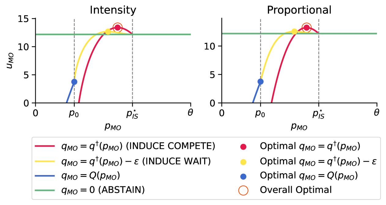
Figure 3: Visualization of $\mathtt{MO}$’s utility for different inventory-setting strategies. Game parameters are $c_{\mathtt{MO}}=4$, $c_{\mathtt{IS}}=2$, $\alpha=0.2$, $k=2$, and $\theta=10$.

4.3 Practical implications

Having now computed the equilibrium, we can answer questions about $\mathtt{MO}$’s optimal actions and the corresponding equilibrium in different situations. For all plots, we use $\theta=10$. The square phase diagrams are constructed by computing the equilibrium for a $200\times 200$ grid of the x-axis and y-axis parameters.

How does the equilibrium change depending on the relative costs of the two sellers?

Figure 4 characterizes the equilibrium for different combinations of $c_{\mathtt{MO}}$. We mark $\theta(1-\alpha)$ on the $c_{\mathtt{IS}}$ axis because this is a critical threshold at which $p_{0}=\theta$; above this threshold, $\mathtt{IS}$ always abstains regardless of what the $\mathtt{MO}$ does, as described in Section 2. In Figure 4, we observe that when $c_{\mathtt{MO}}$ is high and $c_{\mathtt{IS}}$ is low, $\mathtt{MO}$ will prefer to let $\mathtt{IS}$ sell and $\mathtt{MO}$ will induce $\mathtt{IS}$ to compete. When $c_{\mathtt{IS}}$ is relatively large, $\mathtt{MO}$ will prefer to sell themselves and $\mathtt{IS}$ will be induced to abstain. There is also a small region where $\mathtt{MO}$ and $\mathtt{IS}$ have roughly equal costs in which $\mathtt{MO}$ finds it optimal to induce $\mathtt{IS}$ to wait. Relating back to the concept of de-monopolization, note that red regions in both plots and the yellow region in the intensity rationing (left) plot correspond to regions where $\mathtt{IS}$ is de-monopolized at equilibrium. Could write this as a corollary in the previous section Figure 5 visualizes the corresponding prices and quantities. We observe that for the ($c_{\mathtt{MO}}$, $c_{\mathtt{IS}}$) combinations that fall in the red “$\mathtt{IS}$ competes” region in Figure 4, $\mathtt{MO}$ induces compete by buying only a small quantity, which is enough to induce $\mathtt{IS}$ to set a slightly lower price than they would otherwise. Figure 6 shows the corresponding utilities. We see that the marketplace operator can achieve high utility when their own cost $c_{\mathtt{MO}}$ is low, but they can also achieve high utility whenever the independent seller’s cost $c_{\mathtt{IS}}$ is low.

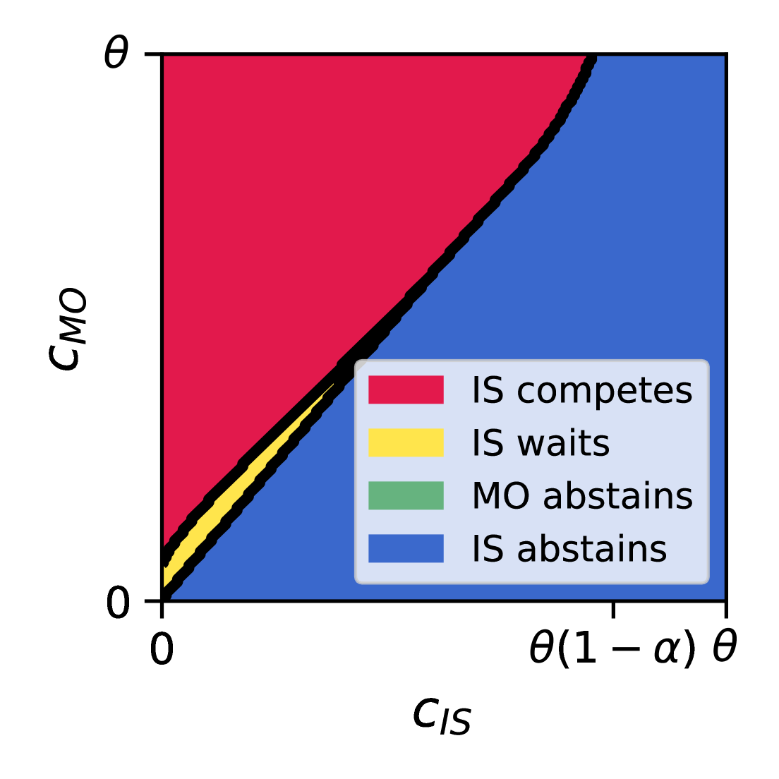
(a) Intensity

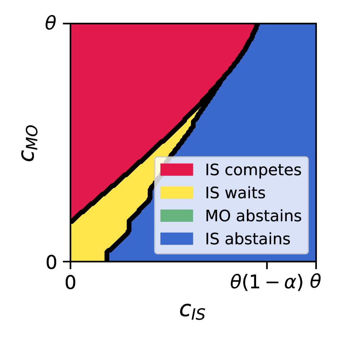
(b) Proportional

Figure 4: Equilibrium characterization for each ($c_{\mathtt{MO}},c_{\mathtt{IS}}$) combination under different rationing rules when $\alpha=0.2$ and $k=2$. Red denotes cost combinations where it is optimal for $\mathtt{MO}$ to induce $\mathtt{IS}$ to compete. Blue regions are where $\mathtt{MO}$ sets a price that causes $\mathtt{IS}$ to abstain. Yellow regions are where $\mathtt{MO}$ finds it optimal to induce $\mathtt{IS}$ to wait. Green is used to denote regions are where $\mathtt{MO}$ chooses to abstain, but no such regions exist in the plots.

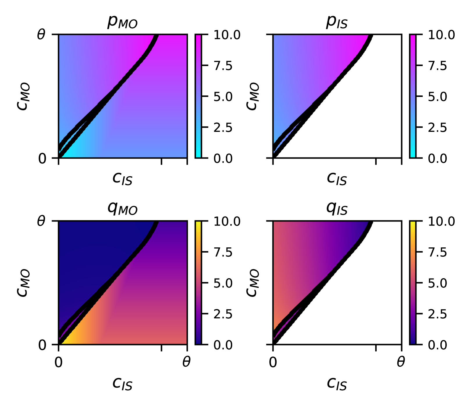
(a) Intensity

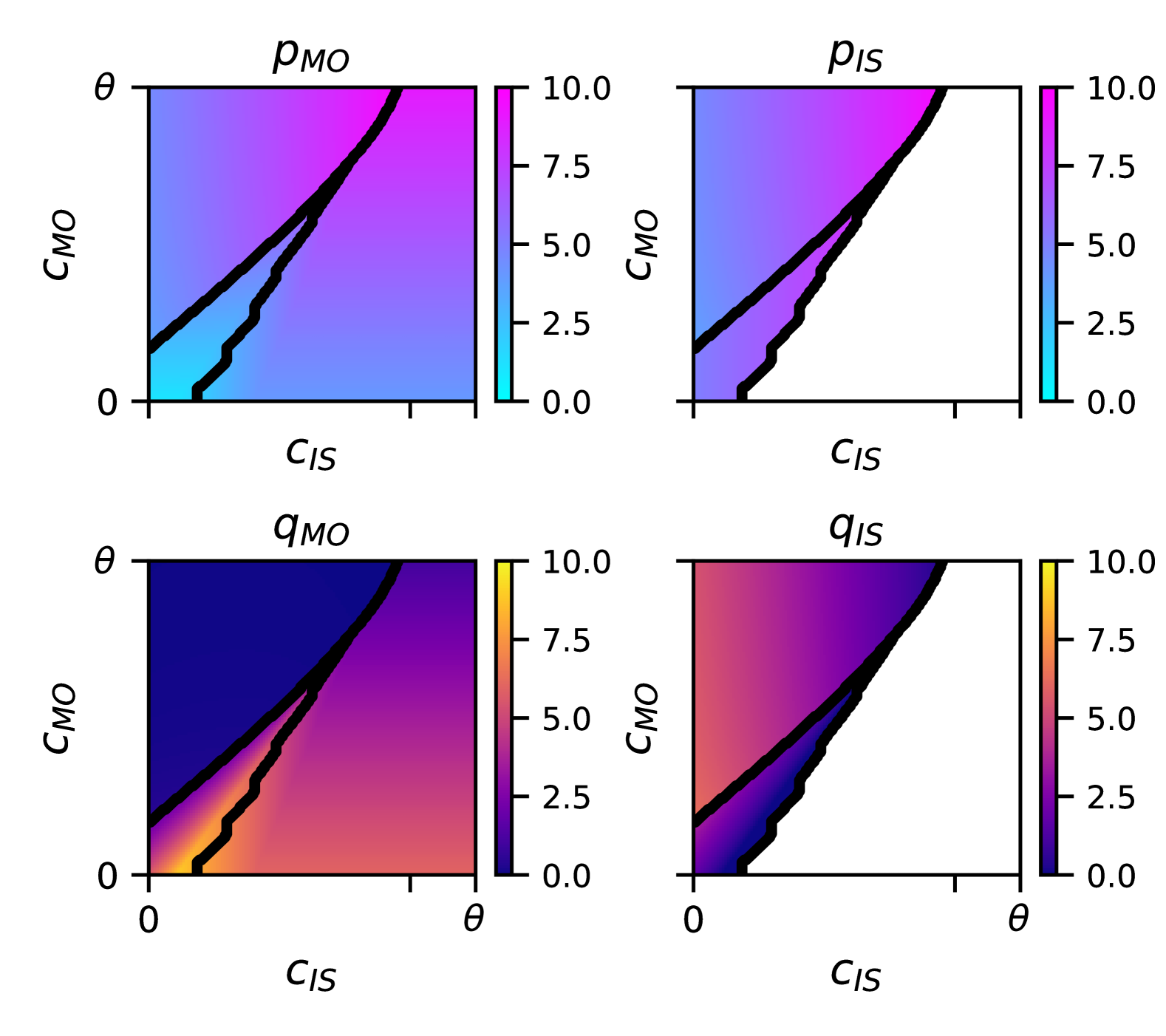
(b) Proportional

Figure 5: $\mathtt{MO}$ and $\mathtt{IS}$’s equilibrium prices and quantities for each ($c_{\mathtt{MO}},c_{\mathtt{IS}}$) combination under different rationing rules when $\alpha=0.2$ and $k=2$. Regions where a player abstains (by setting their quantity to zero) are white.

(a) Intensity

(b) Proportional

Figure 6: Utilities of $\mathtt{MO}$ and $\mathtt{IS}$ for each ($c_{\mathtt{MO}},c_{\mathtt{IS}}$) combination under different rationing rules when $\alpha=0.2$ and $k=2$.

How should the marketplace operator set $\alpha$?

Suppose that instead of treating the referral fee $\alpha$ as fixed, we allow $\mathtt{MO}$ to choose an $\alpha\in[0,1]$ before the game begins. What value results in the highest utility for the marketplace operator? Figure 7 sheds light on this question. Even though increasing $\alpha$ increases the revenue $\mathtt{MO}$ gets for each unit sold by $\mathtt{IS}$, $\mathtt{MO}$ should not in general set $\alpha$ as high as possible. This is because for large values of $\alpha$, the independent seller will only be willing to set a high price and sell few units, or will not be willing to sell at all, so $\mathtt{MO}$ cannot experience the benefits of having $\mathtt{IS}$ in the market. It is worth pointing out that the optimal $\alpha$ is generally not the largest $\alpha$ such that $\mathtt{IS}$ competes instead of abstains (represented by the right end of the pink highlighting in Figure 7); the value that maximizes $u_{\mathtt{MO}}$ is somewhat smaller.

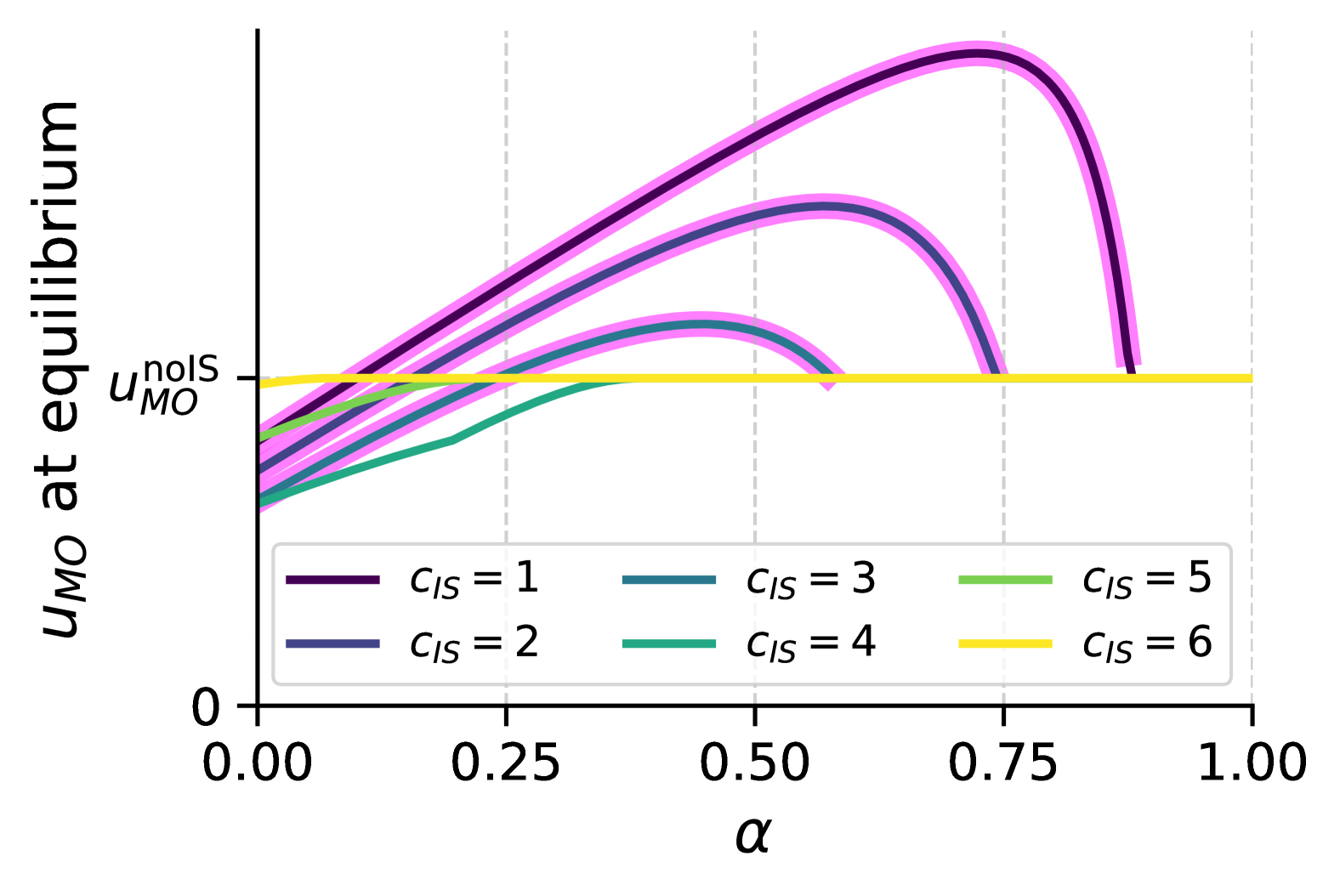
(a) Intensity

(b) Proportional

Figure 7: $\mathtt{MO}$’s utility at equilibrium as $\alpha$ is varied under different rationing rules. $u_{\mathtt{MO}}^{\text{noIS}}$ marks the utility $\mathtt{MO}$ would receive if $\mathtt{IS}$ were not in the market. Pink highlighting means that $\mathtt{IS}$ competes at the equilibrium induced by those game parameters. The other game parameters are fixed at $c_{\mathtt{MO}}=5$ and $k=2$.

Should $\mathtt{MO}$ behave differently when selling a product with a larger impact on customer experience (large $k$)?

Certain products are more important in determining whether a customer is likely to return to the marketplace in the future. For example, being able to reliably purchase essential household staples at a marketplace can have a positive effect on customer retention. In our model, such products are modeled as having a large value of $k$. Figure 8 shows the equilibrium strategies that result from different combinations of $k$ and the independent seller’s cost $c_{\mathtt{IS}}$ under intensity rationing. The plots for proportional rationing look similar and are deferred to Appendix D. Observe that often $q_{\mathtt{MO}}$ increases as $k$ increases. This is true even when $\mathtt{MO}$ is using their inventory to induce $\mathtt{IS}$ to compete rather than selling directly themselves; in such cases, a larger $q_{\mathtt{MO}}$ can induce $\mathtt{IS}$ to set a lower price and sell more inventory. This leads to more satisfied customers, which contributes to marketplace health and benefits $\mathtt{MO}$.

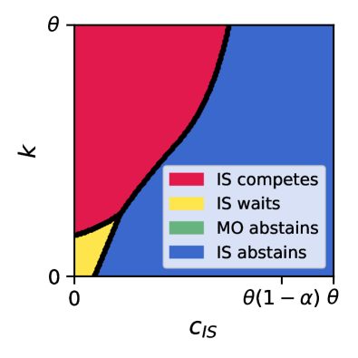
(a) Equilibrium characterization

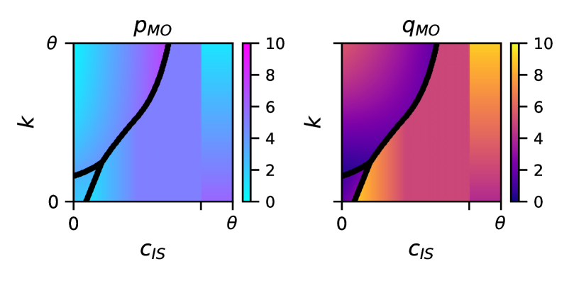
(b) $\mathtt{MO}$’s equilibrium strategies

Figure 8: Equilibrium characterization and $\mathtt{MO}$’s corresponding strategies for different combinations of $k$ and $c_{\mathtt{IS}}$ under intensity rationing. The other game parameters are fixed at $c_{\mathtt{MO}}=2$ and $\alpha=0.2$.

5 Welfare Implications under Intensity Rationing

One may wonder what effect the marketplace place operator has on overall welfare when they enter the market as a seller. In order to analyze welfare, we must first compute consumer surplus. In order to allow for straightforward computation of consumer surplus, we will assume intensity rationing with perfect substitutes. Recall that this means that the residual demand curve for the lower-priced seller $i$ is given by $R(p_{i})=Q(p_{i})-q_{j}$ (i.e., the original demand curve shifted down by $q_{j}$). Consumer surplus is the sum of excess value that customers who are able to buy the good get from buying the good: suppose that the good is offered at price $p$. Let $v_{i}$ denote customer $i$’s (random) valuation for the good and let $\mathcal{B}$ denote the set customers who bought the good. Then, $\mathrm{CS}={\mathbb{E}}\left[\sum_{i\in\mathcal{B}}(v_{i}-p)\right]$, where the expectation is taken over the randomness in the valuations.

For intensity rationing, we can compute consumer surplus by computing the area of a triangle (plus a trapezoid). More explicitly, for any $(p_{\mathtt{MO}},q_{\mathtt{MO}},p_{\mathtt{IS}},q_{\mathtt{IS}})$ such that $q_{\mathtt{IS}}=D_{\mathtt{IS}}(p_{\mathtt{IS}};q_{\mathtt{MO}},p_{\mathtt{MO}})$, consumer surplus can be computed as

$$\mathrm{CS}(p_{\mathtt{MO}},q_{\mathtt{MO}},p_{\mathtt{IS}},q_{\mathtt{IS}})=\begin{cases}\frac{1}{2}q_{\mathtt{IS}}^{2}&\text{if }p_{\mathtt{IS}}\leq p_{\mathtt{MO}}\\ (\theta-p_{\mathtt{MO}})q_{\mathtt{MO}}-\frac{1}{2}q_{\mathtt{MO}}^{2}+\frac{1}{2}(q_{\mathtt{IS}}-q_{\mathtt{MO}})^{2}&\text{if }p_{\mathtt{IS}}<p_{\mathtt{MO}}.\\ \end{cases}$$

Figure 14 in Appendix E illustrates the consumer surplus for different cases. We define $\mathrm{CS}^{\star}:=\mathrm{CS}(\infty,0,p^{\star}_{\mathtt{IS}},Q(p^{\star}_{\mathtt{IS}}))$ to be the consumer surplus when the marketplace operator does not participate as a seller. The following lemma tells us that $\mathtt{MO}$ entering the market increases consumer surplus.

Lemma 3 (Entry of marketplace operator increases CS).

Under intensity rationing with perfect substitutes, for any $p_{\mathtt{MO}}$ and $q_{\mathtt{MO}}$ (including the equilibrium values), as long as the independent seller best responds, the consumer surplus will be at least as high as if the marketplace operator did not participate as a seller:

$$\mathrm{CS}(p_{\mathtt{MO}},q_{\mathtt{MO}},p_{\mathtt{IS}}^{\mathrm{BR}}(p_{\mathtt{MO}},q_{\mathtt{MO}}),q_{\mathtt{IS}}^{\mathrm{BR}}(p_{\mathtt{MO}},q_{\mathtt{MO}}))\geq\mathrm{CS}^{\star}\qquad\forall p_{\mathtt{MO}},q_{\mathtt{MO}}.$$

The inequality is strict whenever $p_{\mathtt{MO}}<p^{\star}_{\mathtt{IS}}$.

The intuition behind this is that the entry of the marketplace operator induces the independent seller to set a lower price than they would otherwise. Furthermore, we know by Proposition 2 that it is optimal for the independent seller to fully meet their demand at their chosen price. Combining these two facts tells the entry of the operator causes more inventory to be offered at a lower price, which increases consumer surplus. The full proof is given in Appendix E.

We now turn our attention to total welfare, which can be computed as

$$W(p_{\mathtt{MO}},q_{\mathtt{MO}},p_{\mathtt{IS}},q_{\mathtt{IS}})=\mathrm{CS}(p_{\mathtt{MO}},q_{\mathtt{MO}},p_{\mathtt{IS}},q_{\mathtt{IS}})+u_{\mathtt{MO}}(p_{\mathtt{MO}},q_{\mathtt{MO}},p_{\mathtt{IS}},q_{\mathtt{IS}})+u_{\mathtt{IS}}(p_{\mathtt{MO}},q_{\mathtt{MO}},p_{\mathtt{IS}},q_{\mathtt{IS}}).$$ (5)

Figure 9 visualizes the welfare that results from the combinations of game parameters considered in Figures 4 and 5. We remark that this plot is representative of plots for all game parameters and we defer the plots of the difference under different game parameters to Appendix TODO. For all of these plots, the following observations hold: (1) The total welfare when both $\mathtt{MO}$ and $\mathtt{IS}$ can choose to sell is always at least as high as the welfare when $\mathtt{IS}$ is the sole seller. (2) The largest gain in total welfare occurs when $c_{\mathtt{IS}}$ is large and $c_{\mathtt{MO}}$ is small. This is not surprising because this is the region in which the equilibrium result is that $\mathtt{MO}$ is the only seller.

Proposition 6.

Something about how when $\mathtt{MO}$ has the option to sell , total welfare increases or stays the same (compared to when $\mathtt{IS}$ is the only seller).

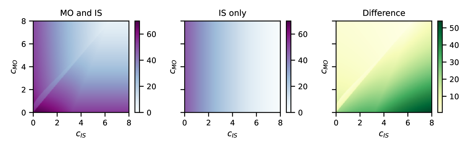
Figure 9: Welfare for different $c_{\mathtt{MO}}$ and $c_{\mathtt{IS}}$ combinations at the two-player equilibrium (left) and if only $\mathtt{IS}$ is able to sell (middle). The difference (Both - $\mathtt{IS}$ only) is on the right. The game parameters are the same as in Figures 4 and 5. The minimum and maximum values of each colorbar correspond to the minimum and maximum values in the data being displayed.

6 Extension to Imperfect Substitutability

Intensity rationing, proportional rationing, and inverse intensity rationing allIntensity rationing and proportional rationing implicitly assume that the two players are selling perfectly substitutable goods. What if instead their goods are imperfect substitutes? As special cases of the residual demand function classes we introduced, it is straightforward to model a form of one-directional imperfect substitutability. Let $\gamma\in[0,1]$ be a substitutability parameter, where $\gamma=1$ recovers perfect substitutes and $\gamma=0$ means that the two goods are not at all substitutable. For each of the threetwo rationing rules, we can obtain the imperfect substitutes version of the residual demand function for Player $i$ by replacing $q_{j}$ with $\gamma q_{j}$. For intensity rationing, this yields

$$R(p_{i};q_{j})=\theta-p_{i}-\gamma q_{j}.$$ (6)

For proportional rationing, this yields

$$R(p_{i};q_{j},p_{j})=(\theta-p_{i})\left(1-\frac{\gamma q_{j}}{Q(p_{j})}\right).$$ (7)

For inverse intensity rationing, this yields

$$R(p_{i};q_{j})=\min(\theta-p_{i},\theta-\gamma q_{j})$$ (8)

Interpretation. The effect of the inventory of the lower-priced seller $i$ on the higher-priced seller $j$ is now damped by a $\gamma$ factor. Player $i$’s demand function is not affected by $\gamma$; only $\mathtt{IS}$’s residual demand function is affected (hence “one-directional” imperfect substitutability). The interpretation is something like this: Each consumer initially wants both Player $i$’s good and Player $j$’s good and assigns the same valuation $v$ to both (this valuation is randomly sampled from $\mathrm{Unif}([0,\theta])$. If they buy the good from Player $i$, then with probability $\gamma$ they will no longer want the good from Player $j$. Otherwise, they keep their original valuation, and they buy from Player $j$ if $v\geq p_{i}$. Which customers are able to buy from $\mathtt{MO}$ is determined by the rationing rule.

We emphasize the limitations of this model, which we chose for its mathematical elegance and not because it is necessarily the most realistic model of imperfect substitutability. Traditional models of markets of differentiated products (see Chapter 6 of Vives (1999)) generally start with defining the utility function $U(q_{1},q_{2})$ of a representative consumer and then maximizing the net utility: $\max_{q_{1},q_{2}}U(q_{1},q_{2})-p_{1}q_{1}-p_{2}q_{2}$. The first-order conditions yield the inverse demands $p_{i}=\frac{\partial}{\partial q_{i}}U(q_{1},q_{2})$ for $i=1,2$. Solving this system for $q_{i}$’s yields the direct demands. This approach is nice because it derives demand curves from first principles. Deriving equilibria for such models is out of scope for this paper but is a good direction for future work.

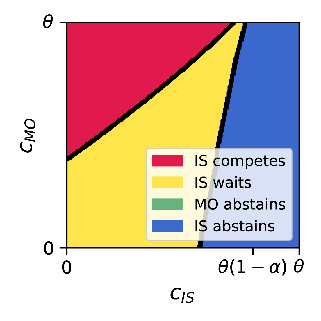
(a) Intensity

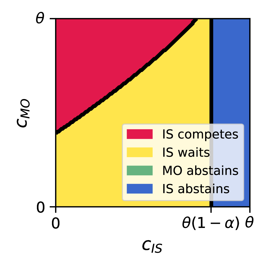
(b) Proportional

Figure 10: Equilibrium strategies for different $c_{\mathtt{MO}},c_{\mathtt{IS}}$ combinations in the same setting as Figure 4 except with $\gamma=0.5$ (imperfect substitutability) rather than $\gamma=1$ (perfect substitutability).

Observe that (6) is a subtractive residual demand function with $f(q_{j})=\gamma q_{j}$, (7) is a multiplicative residual demand function with $g(q_{j})=1-\gamma q_{j}/Q(p_{j})$, and (8) is a truncated residual demand function with $h(q_{j})=\gamma q_{j}$.Observe that (6) is a subtractive residual demand function with $f(q_{j})=\gamma q_{j}$ and (7) is a multiplicative residual demand function with $g(q_{j})=1-\gamma q_{j}/Q(p_{j})$, which both satify Assumption 3. Thus, the results derived in Section 4 apply directly.

Figure 10 visualizes the equilibrium strategies for $\gamma=0.5$. Compared to Figure 4, which is the same setting but with $\gamma=1$, we see a larger yellow region (corresponding to $\mathtt{IS}$ waiting it out) in the imperfect substitutes setting.

7 Conclusion

In this paper, we formulate an asymmetric price-quantity Stackelberg game that can be used to model a marketplace with a marketplace operator and an independent seller. We now summarize some of the key practical takeaways.

1) Inducing competition. In order to induce $\mathtt{IS}$ to compete on price, $\mathtt{MO}$ must both (1) set $p_{\mathtt{MO}}$ between $\mathtt{IS}$’s break-even price $p_{0}$ and sole-seller price $p^{\star}_{\mathtt{IS}}$, and (2) buy sufficient inventory to back it up (Section 3). The inventory threshold is smallest if high-valuation customers buy first and largest if low-valuation customers buy first. This leads to the question of when it is optimal for $\mathtt{MO}$ to induce competition. Under intensity and proportional rationing, we observe that inducing compete is utility-maximizing for $\mathtt{MO}$ when $c_{\mathtt{IS}}$ is small and $c_{\mathtt{MO}}$ is relatively large (Figure 4). This is often the case in the real world since independent sellers who specialize in a single product can likely achieve lower per-unit costs than a platform that sells many products.

2) Setting the fee $\alpha$. Marketplace operators generally have control of the referral fee $\alpha$ that is charged to sellers. Although increasing $\alpha$ increases the per-unit revenue that $\mathtt{MO}$ receives from $\mathtt{IS}$, this also causes $\mathtt{IS}$ to sell fewer units so $\mathtt{MO}$ misses out on the referral fee and additional benefit $k$ for those units that would have been sold had $\alpha$ been lower. Furthermore, when $\alpha$ is so high that $c_{\mathtt{IS}}/(1-\alpha)\geq\theta$, $\mathtt{IS}$ cannot make a profit and will not sell at all. For these reasons, $\mathtt{MO}$ should not simply set $\alpha$ as large as possible and should instead keep $\mathtt{IS}$’s own strategic behavior in mind when setting $\alpha$ (Figure 7).

3) Consumer surplus and welfare. Under intensity rationing, when the marketplace operator enters the marketplace as a seller, this improves consumer surplus and total welfare (Lemma 3 and Figure 9).

I think it may be more effective to refer to the limitations/assumptions in the text (I already added it for the salvage value comment) and focus this section only on future directions.

Limitations and Future Directions.

There are many ways to extend the work we present. We now list several. (1) Multiple third-party sellers. Our current analysis relies on the assumption that once a seller runs out of inventory, all remaining customers can only buy from the remaining seller. However, if there are multiple third-party sellers, there may be additional inter-seller competition, possibly requiring new analysis. (2) Replacing $k$ with a multiplier of consumer surplus. Recall that $k$ is meant to model the marketplace operator’s extra benefit (beyond the immediate monetary benefit) that arises from a customer’s satisfaction for having made a purchase. Our current model represents this as a flat per-unit utility. However, it is arguably more realistic to model $k$ as dependent on price or as a multiplier of consumer surplus, since a customer who buys a product at $5 is likely happier than a customer who buys a product at $10 and is more likely to return to the platform and make more purchases. (3) Positive salvage value. This work implicitly assumes that a player’s leftover inventory has zero salvage value. In reality, products that have steady demand generally have positive salvage value because excess inventory can be sold in the next time period. (4) Non-linear demand. We assume a linear demand in our paper, and it would be useful to verify whether our findings hold under other demand functions (e.g., Cobb-Douglas) as a robustness check. (5) Integer-constrained inventory. Our model assumes quantity is continuous and that fractional amounts of inventory can be ordered. In reality, inventory quantities are often integers. It is worth investigating whether anything unexpected happens if quantities are restricted to be integer-valued. (6) Endogenous timing. Suppose a platform can choose between the Stackelberg game that we analyze in this paper and a simultaneous game (where $\mathtt{MO}$ and $\mathtt{IS}$ make their decisions at the same time). Which game yields higher utility to $\mathtt{MO}$? (7) Welfare under other rationing rules. Investigating the welfare implications under rationing rules other than intensity rationing with perfect substitutability is important from a practical perspective, as many products have demand rationed in other ways.

Appendix A Discussion of Rationing Rules

In this section we provide an in-depth discussion of rationing rules. In Section A.1 we provide relevant background on demand functions and explain why we choose to not study inverse intensity rationing. In Section A.2, we provide examples of intensity, proportional, and inverse intensity rationing. In Section A.3, we describe the probabilistic modeling assumptions underlying proportional rationing and show how the residual demand function is derived starting from these assumptions. In Section A.4, we show that, although the assumptions of proportional rationing are not entirely natural, the implied residual demand function is very similar to the residual demand function that we arrive at under more natural assumptions.

A.1 Background

For additional discussions of rationing rules, see Section 14.2 of Rasmusen (1989), Section 5.3.1 of Tirole (1988), and Section 2 of Davidson and Deneckere (1986). The last describes a perspective on demand functions and rationing rules that views demand functions as arising from individual consumers each with their own identical demand curve. We will instead view demand functions as arising a population of customers with heterogeneous valuations who each wish to purchase one unit of the good, as presented in Section 4.1.1 of Vohra and Krishnamurthi (2012).

Demand functions. Before describing rationing rules, we will review some background on demand functions. A demand function $Q(p)$ tells you the expected number of people who will buy a good at price $p$. Specifically, assume that there are $n$ total customers, and each customer $i$ has a valuation $v_{i}$ (a.k.a. the maximum price they are willing to pay, a.k.a. their reservation price) that is an independent random variable sampled iid from some common distribution. Then the demand function is

$$Q(p) =\sum_{i=1}^{n}{\mathbb{E}}[\mathbbm{1}{\left\{v_{i}\geq p\right\}}]$$

$$=\sum_{i=1}^{n}{\mathbb{P}}(v_{i}\geq p)$$

$$=n{\mathbb{P}}(v_{1}\geq p)\quad\text{since $v_{i}$'s are iid}.$$

If we assume that the distribution of the valuations is uniform, this induces a linear demand function: if $v_{i}\sim\text{Unif}([0,\theta])$, then ${\mathbb{P}}(v_{1}\geq p)=(\theta-p)/\theta$ for $p\in[0,\theta]$. This allows us to write the demand function as

$$Q(p,\theta)=\begin{cases}n-\frac{n}{\theta}p&\text{for $0\leq p\leq\theta$}\\ 0&\text{for $p>\theta$}.\end{cases}$$

If $n=\theta$, this further simplifies to $Q(p)=\theta-p$, which is the demand function we consider, as described in Assumption 1.

A remark on inverse intensity rationing. One type of rationing that has appeared in the literature but we do not consider is inverse intensity rationing, also known as inefficient rationing (Rasmusen, 1989). This rationing scheme assumes that the lowest valuation customers buy first, yielding the residual demand function

$$R(p_{i})=\min\big{(}Q(p_{i}),\theta-q_{j}\big{)}.$$

This is visualized in Figure 11. We choose not to study this type of rationing rule due to its logical weaknesses. When we think about the inverse intensity rationing from the perspective of individual buyers, the underlying assumption seems to imply irrational behavior. Specifically, it requires that we assume that the buyers with the lowest valuation buy the good first, even if their valuation does not exceed the price. This leads to weird behavior when we attempt to use this rationing rule in our analysis, because it implies the creation of demand that is not captured by the original demand curve. A more realistic alternative to inverse intensity rationing would be to assume that the customers with the lowest valuation above the price are the first to buy. This would lead to an $R$ that has a vertical drop from price $p_{i}+q_{j}$ down to $p_{i}$ and then has slope $-1$ from price $p$ down to zero. In other words, it looks like $Q(p)$ until price $p_{i}+q_{j}$ and then matches intensity rationing from price $p_{i}$ down.

Figure 11: Visualization of the residual demand function $R(p_{\mathtt{IS}})$ for $\theta=4$, $q_{\mathtt{MO}}=1$, and $p_{\mathtt{MO}}=2$ under inverse intensity rationing.

A.2 Examples of each rationing rule

Recall that rationing rules are essentially an assumption about the order in which customers arrive. The customers who arrive earliest have first pick between the lower-priced seller and higher-priced seller and since we assume that the customers are utility maximizing, they will purchase from the lower-priced seller as long as they have inventory. Intensity rationing assumes that customers arrive in order of descending willingness to pay. Proportional rationing (roughly) assumes that the arrival order is independent of valuation. Inverse intensity rationing assumes that customers arrive in order of ascending willingness to pay.

Example of intensity rationing. Customers who want a product the most will (if the product is sold online) refresh the page most recently or (if the product is sold in person), be willing to wait in a long line on the product launch date. Thus the customers with the highest willingness to pay get the earliest access to the product and are able to buy the lower-priced version before it goes out of stock. For example, people wait in line to buy iPhones on their release dates (Molina, 2021).

Example of proportional rationing. Before presenting our example, we remark that one peculiarity about proportional rationing is that the probability that a customer is routed to the lower-priced seller is increasing in the lower-priced seller’s inventory. Once a customer is routed to seller, they must choose whether to buy from that seller and have no ability to switch to the other seller. We now present a stylized example that satisfies this: suppose there are two hot dog chains, Cheap Dogs and Fancy Dogs. Each chain has many hot dog carts scattered across the city and each chain’s inventory is proportional to their number of carts. People walk around the city and when they get hungry, they buy a hotdog from the first stand they encounter. If the first stand they go to does not offer a hotdog a price they are happy with, they become so dejected that they no longer want to eat a hotdog, so there is no transfer of demand from a higher-priced seller to a lower-priced seller.

Example of inverse-intensity rationing. Suppose a new product is being released and consumers initially do not know whether it is worth buying, so the first consumers to buy the good are not willing to pay much for it. However, once the early adopters ascertain that the good is high quality, they spread the word to other consumers who are then willing to pay more for the product. This is the reason that new companies and products frequently offer coupons to attract customers.

A.3 Derivation of residual demand function under proportional rationing

In this section, we describe the probabilistic modeling assumptions that underlie proportional rationing. Under proportional rationing, each customer is randomly assigned to the higher price with some probability $\rho$ and the lower price with probability $1-\rho$. There is a total population of $n=\theta$ customers. $\rho$ is such that in expectation the demand that the lower-priced seller faces at their price $p_{j}$ is exactly equal to their supply $q_{j}$, which is

$$\rho=\frac{Q(p_{j})-q_{j}}{Q(p_{j})}.$$

The full probabilistic model is: There are $\theta$ customers each with valuation $v_{i}\sim\mathrm{Unif}([0,\theta])$. Independent of their valuation, the customer is sent to the higher-priced seller with probability $\rho$; otherwise they are sent to the lower-priced seller. Customers either buy at the seller they are sent to or do not buy at all. Given this model, the expected demand that the higher-priced seller faces when setting price $p$ and the lower-priced seller sets price $p_{j}$ and quantity $q_{j}$ is

$$R(p;q_{j},p_{j}) ={\mathbb{E}}\left[\sum_{i=1}^{n}\mathbbm{1}{\left\{v_{i}\geq p\right\}}\mathbbm{1}{\left\{i\text{ assigned to high price seller}\right\}}\right]$$

$$=\sum_{i=1}^{n}{\mathbb{E}}\left[\mathbbm{1}{\left\{v_{i}\geq p\right\}}\mathbbm{1}{\left\{i\text{ assigned to high price seller}\right\}}\right]\qquad\text{linearity of expectation}$$

$$=\sum_{i=1}^{n}{\mathbb{E}}[\mathbbm{1}{\left\{v_{i}\geq p\right\}}]{\mathbb{E}}[\mathbbm{1}{\left\{i\text{ assigned to high price seller}\right\}}]\qquad\text{independence}$$

$$=\sum_{i=1}^{n}{\mathbb{P}}(v_{i}\geq p){\mathbb{P}}(i\text{ assigned to high price seller})$$

$$=n\frac{\theta-p}{\theta}\rho$$

$$=(\theta-p)\rho=(\theta-p)\frac{Q(p_{j})-q_{j}}{Q(p_{j})}=Q(p)\frac{Q(p_{j})-q_{j}}{Q(p_{j})}\qquad\text{since $n=\theta$}.$$

A.4 Realism of proportional rationing

As previously described, the assumptions underpinning proportional rationing are a bit peculiar. We adopt this rationing rule in the main paper because it leads to an analytical residual demand function that is easy to work with and is also the convention in existing literature. In this section, we analyze an alternative to proportional rationing based on more realistic assumptions and find it generally produces residual demand functions that are very similar to those under proportional rationing.

More realistic assumptions. There are $n=\theta$ total customers. Assume that customers arrive one at a time and their valuation is sampled $v_{i}\sim\text{Unif}([0,\theta])$. A customer purchases the product if the lowest price available does not exceed their valuation. Otherwise, they leave immediately (whether they leave or wait for a lower price does not matter in practice, because the price only ever goes up after one seller runs out).

We will derive the residual demand function for the higher-priced seller. Let $\text{NegBin}(r,p)$ denote the probability distribution corresponding to the number of trials needed to get $r$ successes from flipping a coin with bias $p$, which has probability mass function $f(k)={k-1\choose r-1}p^{r}(1-p)^{k-r}$. Let $N\sim\text{NegBin}(q_{j},\frac{\theta-p_{j}}{\theta})$ be the number of customers that would have to arrive in order for all of the lower-priced seller’s inventory to be exhausted. Let $M=\max(\theta-N,0)$ be the number of buyers who have not yet visited the website after the lower-priced seller sells out and let $V_{1},...,V_{M}$ denote the valuations of the customers that arrive after the lower-priced seller has sold out. Then the residual demand is

$$R(p) ={\mathbb{E}}_{M}\left[{\mathbb{E}}_{V_{1},...,V_{M}}\left[\sum_{i=1}^{M}\mathbbm{1}{\left\{V_{i}\geq p\right\}}\Big{|}M\right]\right]\quad\text{by tower property}$$

$$={\mathbb{E}}_{M}\left[{M\frac{\theta-p}{\theta}}\right]\quad\text{by linearity of expectation}$$

$$=\frac{\theta-p}{\theta}{\mathbb{E}}[M]$$

$$=\frac{\theta-p}{\theta}{\mathbb{E}}[\max(\theta-N,0)]$$

$$=\frac{\theta-p}{\theta}\sum_{k=q_{j}}^{\theta}(\theta-k){k-1\choose q_{j}-1}\left(\frac{p_{j}}{\theta}\right)^{k-q_{j}}\left(\frac{\theta-p_{j}}{\theta}\right)^{q_{j}}.$$

Figure 12 illustrates that when the lower-priced seller’s quantity $q_{j}$ is small relative to demand at price their $p_{j}$, the residual demand under our more realistic assumptions is visually identical to under proportional rationing. The difference between the two curves only becomes pronounced when $q_{j}$ approaches $Q(p_{j})$.

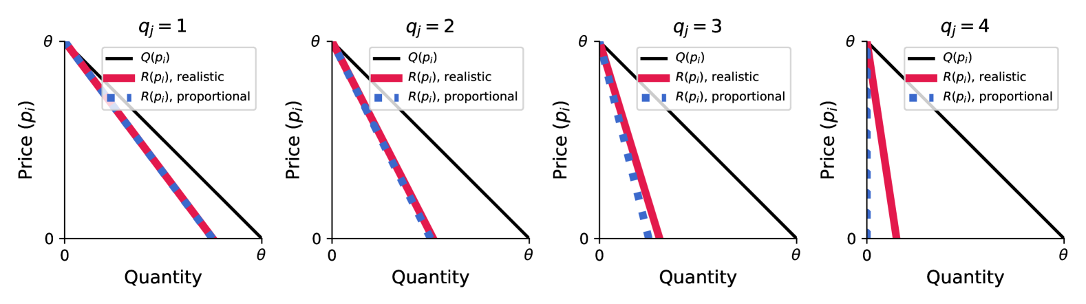
Figure 12: Comparison of residual demand function under proportional rationing and under the more realistic assumptions described in Appendix A.4. $p_{j}$ is set to 6, so the corresponding original demand is $Q(p_{j})=\theta-6=4$.

Appendix B Proofs for Section 3

Proof of Proposition 3.

We first argue that the optimal $p_{\mathtt{IS}}\leq p_{\mathtt{MO}}$ is $p_{\mathtt{IS}}=p^{\star}_{\mathtt{IS}}$. Since we assumed $p^{\star}_{\mathtt{IS}}\leq p_{\mathtt{MO}}$, we have $p^{\star}_{\mathtt{IS}}=\arg\max_{p}((1-\alpha)p-c_{\mathtt{IS}})Q(p)=\arg\max_{p\leq p_{\mathtt{MO}}}((1-\alpha)p-c_{\mathtt{IS}})Q(p)$, where the first equality is the definition of $p^{\star}_{\mathtt{IS}}$ and the second equality comes from the fact that the maximizer of a set is the maximizer of any subset containing the maximizer.

Let $u_{\mathtt{IS}}(p)$ denote $\mathtt{IS}$’s utility when they set price $p$ and buy inventory to exactly meet their demand at that price. We now show that $u_{\mathtt{IS}}(p^{\star}_{\mathtt{IS}})>u_{\mathtt{IS}}(p_{\mathtt{IS}})$ whenever $p_{\mathtt{IS}}\geq p_{\mathtt{MO}}$. Consider any $p_{\mathtt{IS}}\geq p_{\mathtt{MO}}$. Then,

$$u_{\mathtt{IS}}(p^{\star}_{\mathtt{IS}}) =[(1-\alpha)p^{\star}_{\mathtt{IS}}-c_{\mathtt{IS}}]Q(p^{\star}_{\mathtt{IS}})$$

$$>[(1-\alpha)p_{\mathtt{IS}}-c_{\mathtt{IS}}]Q(p_{\mathtt{IS}})\qquad\text{since $p^{\star}_{\mathtt{IS}}$ is the unique maximizer}$$

$$\geq[(1-\alpha)p_{\mathtt{IS}}-c_{\mathtt{IS}}]R(p_{\mathtt{IS}})\qquad\text{Assumption \ref{assumption:R}(a)}$$

$$=u_{\mathtt{IS}}(p_{\mathtt{IS}}).$$

We have shown that $p^{\star}_{\mathtt{IS}}$ is the optimal $p_{\mathtt{IS}}$ among $p_{\mathtt{IS}}\leq p_{\mathtt{MO}}$ and it achieves higher utility than any $p_{\mathtt{IS}}\geq p_{\mathtt{MO}}$, so it is the global maximizer of utility. ∎

Proof of Proposition 4.

Recall that $\mathtt{IS}$ has three strategies to choose from: abstain, compete, or wait. Whenever $p_{\mathtt{MO}}\geq p_{0}$, $\mathtt{IS}$ can achieve non-negative utility by competing, so they will never abstain. Thus, to determine what $\mathtt{IS}$ will do, we simply have to determine whether it is better for them to compete or wait.

1. Optimal “compete” utility. In order to compete, $\mathtt{IS}$ must set $p_{\mathtt{IS}}\leq p_{\mathtt{MO}}$. The optimal $p_{\mathtt{IS}}$ satisfying this condition is

   $$p_{\mathtt{IS}}^{C} :=\arg\max_{p_{\mathtt{IS}}\leq p_{\mathtt{MO}}}u_{\mathtt{IS}}(p_{\mathtt{IS}};p_{\mathtt{MO}},q_{\mathtt{MO}})$$

   $$=\arg\max_{p_{\mathtt{IS}}\leq p_{\mathtt{MO}}}\underbrace{((1-\alpha)p_{\mathtt{IS}}-c_{\mathtt{IS}})(\theta-p_{\mathtt{IS}})}_{:=u^{C}(p_{\mathtt{IS}})}$$

   $$=p_{\mathtt{MO}}$$

   where the last equality comes from combining the following facts: (1) $p^{\star}_{\mathtt{IS}}$ is the unconstrained maximizer of $u^{C}(p_{\mathtt{IS}})$; (2) the conditions of the proposition assume $p_{\mathtt{MO}}\in[p_{0},p^{\star}_{\mathtt{IS}})$; and (3) $u^{C}(p_{\mathtt{IS}})$ is convex so the $p_{\mathtt{IS}}$ in the constraint set that is closest to the unconstrained maximizer must be constrained maximizer. When $\mathtt{IS}$ sets $p_{\mathtt{MO}}$, they get utility

   $$u_{C}^{*}:=u^{C}(p_{\mathtt{IS}}^{C})=((1-\alpha)p_{\mathtt{MO}}-c_{\mathtt{IS}})(\theta-p_{\mathtt{MO}}).$$

   Note that the optimal compete utility does not depend on the residual demand function because when $\mathtt{IS}$ competes, they do not face the residual demand function.

2. Optimal utility when facing $R$ (upper bound on optimal “wait” utility). To derive the optimal “wait” utility, we would have to solve

   $$\max_{p_{\mathtt{IS}}>p_{\mathtt{MO}}}((1-\alpha)p_{\mathtt{MO}}-c_{\mathtt{IS}})R(p_{\mathtt{IS}};q_{\mathtt{MO}},p_{\mathtt{MO}}).$$

   Rather than solving this constrained optimization problem, we solve the unconstrained optimization problem (for reasons to be explained shortly):

   $$\max_{p_{\mathtt{IS}}}((1-\alpha)p_{\mathtt{MO}}-c_{\mathtt{IS}})R(p_{\mathtt{IS}};q_{\mathtt{MO}},p_{\mathtt{MO}}).$$

   Lemma 4 gives the $p_{\mathtt{IS}}$ that solves this for each class of residual demand functions. Call this $p_{\mathtt{IS}}^{R}$ and let

   $$u^{*}_{R}:=((1-\alpha)p_{\mathtt{IS}}^{R}-c_{\mathtt{IS}})R(p_{\mathtt{IS}}^{R};q_{\mathtt{MO}},p_{\mathtt{MO}})$$

   denote the maximal value achieved by the unconstrained optimization problem.

We now make the following observation:

$\mathtt{IS}$ gets higher utility from waiting than competing if and only if $u^{*}_{R}>u^{*}_{C}$.

This is stated formally and proven in Lemma 5. Thus, to determine whether it is optimal for $\mathtt{IS}$ to wait by setting $p_{\mathtt{IS}}^{R}$ or compete by setting $p_{\mathtt{IS}}^{C}$, we simply have to check if $u^{*}_{R}>u^{*}_{C}$. For each class of residual demand functions, we will solve this condition for $q_{\mathtt{MO}}$ by plugging in the optimal $p_{\mathtt{IS}}$ values derived in Lemma 4.

1. Subtractive demand functions. First, observe that $u_{R}^{*}$ for subtractive demand functions can be written as

   $$u_{R}^{*} =\left((1-\alpha)\left(p^{\star}_{\mathtt{IS}}-\frac{f(q_{\mathtt{MO}})}{2}\right)-c_{\mathtt{IS}}\right)\left(\theta-\left(p^{\star}_{\mathtt{IS}}-\frac{f(q_{\mathtt{MO}})}{2}\right)-f(q_{\mathtt{MO}})\right)$$

   $$=(1-\alpha)\left(p^{\star}_{\mathtt{IS}}-\frac{f(q_{\mathtt{MO}})}{2}-p_{0}\right)\left(\theta-p^{\star}_{\mathtt{IS}}-\frac{f(q_{\mathtt{MO}})}{2}\right)\qquad\text{since $p_{0}=\frac{c_{\mathtt{IS}}}{1-\alpha}$}$$

   $$=(1-\alpha)\left(\frac{p_{0}+\theta}{2}-\frac{f(q_{\mathtt{MO}})}{2}-p_{0}\right)\left(\theta-\frac{p_{0}+\theta}{2}-\frac{f(q_{\mathtt{MO}})}{2}\right)\qquad\text{definition of $p^{\star}_{\mathtt{IS}}$}$$

   $$=(1-\alpha)\left(\frac{\theta}{2}-\frac{p_{0}}{2}-\frac{f(q_{\mathtt{MO}})}{2}\right)\left(\frac{\theta}{2}-\frac{p_{0}}{2}-\frac{f(q_{\mathtt{MO}})}{2}\right)$$

   $$=\frac{(1-\alpha)}{4}(\theta-p_{0}-f(q_{\mathtt{MO}}))^{2}.$$

   Thus,

   $$u_{R}^{*}>u_{C}^{*}\Longleftrightarrow\frac{(1-\alpha)}{4}(\theta-p_{0}-f(q_{\mathtt{MO}}))^{2} >((1-\alpha)p_{\mathtt{MO}}-c_{\mathtt{IS}})(\theta-p_{\mathtt{MO}}).$$

   Solving for $q_{\mathtt{MO}}$, we get

   $$u_{R}^{*}>u_{C}^{*} \Longleftrightarrow f(q_{\mathtt{MO}})<\theta-p_{0}-2\sqrt{(p_{\mathtt{MO}}-p_{0})(\theta-p_{\mathtt{MO}})}.$$

   $$\Longleftrightarrow q_{\mathtt{MO}}<f^{-1}\big{(}\theta-p_{0}-2\sqrt{(p_{\mathtt{MO}}-p_{0})(\theta-p_{\mathtt{MO}})}\big{)}.$$

2. Multiplicative demand functions.

   $$u_{R}^{*}>u_{C}^{*} \Longleftrightarrow((1-\alpha)p^{\star}_{\mathtt{IS}}-c_{\mathtt{IS}})(\theta-p^{\star}_{\mathtt{IS}})g(q_{\mathtt{MO}})>((1-\alpha)p_{\mathtt{MO}}-c_{\mathtt{IS}})(\theta-p_{\mathtt{MO}})$$

   $$\Longleftrightarrow(1-\alpha)(p^{\star}_{\mathtt{IS}}-p_{0})(\theta-p^{\star}_{\mathtt{IS}})g(q_{\mathtt{MO}})>(1-\alpha)(p_{\mathtt{MO}}-p_{0})(\theta-p_{\mathtt{MO}})\quad\text{since $p_{0}=\frac{c_{\mathtt{IS}}}{1-\alpha}$}$$

   $$\Longleftrightarrow(p^{\star}_{\mathtt{IS}}-p_{0})(\theta-p^{\star}_{\mathtt{IS}})g(q_{\mathtt{MO}})>(p_{\mathtt{MO}}-p_{0})(\theta-p_{\mathtt{MO}})$$

   $$\Longleftrightarrow g(q_{\mathtt{MO}})>\frac{(p_{\mathtt{MO}}-p_{0})(\theta-p_{\mathtt{MO}})}{(p^{\star}_{\mathtt{IS}}-p_{0})(\theta-p^{\star}_{\mathtt{IS}})}$$

   $$\Longleftrightarrow q_{\mathtt{MO}}<g^{-1}\left(\frac{(p_{\mathtt{MO}}-p_{0})(\theta-p_{\mathtt{MO}})}{(p^{\star}_{\mathtt{IS}}-p_{0})(\theta-p^{\star}_{\mathtt{IS}})}\right).$$

3. Truncated demand functions. From Lemma 4, we know that if $q_{\mathtt{MO}}$ is low enough that $h(q_{\mathtt{MO}})<p^{\star}_{\mathtt{IS}}$, $\mathtt{IS}$ will wait it out by setting $p_{\mathtt{IS}}=p^{\star}_{\mathtt{IS}}$ and achieve the same utility they would have gotten if they were the sole seller. In the other case where $q_{\mathtt{MO}}$ is high enough that $h(q_{\mathtt{MO}})\geq p^{\star}_{\mathtt{IS}}$, we have

   $$u_{R}^{*}>u_{C}^{*} \Longleftrightarrow((1-\alpha)h(q_{\mathtt{MO}})-c_{\mathtt{IS}})(\theta-h(q_{\mathtt{MO}}))>((1-\alpha)p_{\mathtt{MO}}-c_{\mathtt{IS}})(\theta-p_{\mathtt{MO}})$$

   $$\Longleftrightarrow u^{C}(h(q_{\mathtt{MO}}))>u^{C}(p_{\mathtt{MO}})$$

   Since $$u^{C} p^{\star}_{\mathtt{IS}} u^{C}(h(q_{\mathtt{MO}}))>u^{C}(p_{\mathtt{MO}}) h(q_{\mathtt{MO}}) p^{\star}_{\mathtt{IS}} p_{\mathtt{MO}} p^{\star}_{\mathtt{IS}} h(q_{\mathtt{MO}})-p^{\star}_{\mathtt{IS}}>p^{\star}_{\mathtt{IS}}-p_{\mathtt{MO}} q_{\mathtt{MO}}$$ is a quadratic function with its vertex at , we have if and only if the distance from to is smaller than the distance from to , i.e., if . Solving for gives

   $$\Longleftrightarrow q_{\mathtt{MO}}>h^{-1}(2p^{\star}_{\mathtt{IS}}-p_{\mathtt{MO}})$$

∎

Lemma 4 (Optimal $p_{\mathtt{IS}}$ when facing each $R$).

The solution of

$$\arg\max_{p_{\mathtt{IS}}}u_{R}(p_{\mathtt{IS}})$$ (9)

where $u_{R}(p_{\mathtt{IS}})=((1-\alpha)p_{\mathtt{MO}}-c_{\mathtt{IS}})R(p_{\mathtt{IS}})$ is…

1. For subtractive residual demand function $R(p_{\mathtt{IS}})=\theta-p_{\mathtt{IS}}-f(q_{\mathtt{MO}})$,

   $$p_{\mathtt{IS}}^{\mathrm{sub}}=p^{\star}_{\mathtt{IS}}-\frac{f(q_{\mathtt{MO}})}{2}.$$

2. For multiplicative residual demand function $R(p_{\mathtt{IS}})=(\theta-p_{\mathtt{IS}})g(q_{\mathtt{MO}})$,

   $$p_{\mathtt{IS}}^{\mathrm{mult}}=p^{\star}_{\mathtt{IS}}.$$

3. For truncated residual demand function $R(p_{\mathtt{IS}})=\min(\theta-p_{\mathtt{IS}},\theta-h(q_{\mathtt{MO}}))$,

   $$p_{\mathtt{IS}}^{\mathrm{trunc}}=\begin{cases}p^{\star}_{\mathtt{IS}}&\text{if }p^{\star}_{\mathtt{IS}}>h(q_{\mathtt{MO}})\\ h(q_{\mathtt{MO}})&\text{if }p^{\star}_{\mathtt{IS}}\leq h(q_{\mathtt{MO}})\end{cases}$$

Proof.

Since all of the residual demand functions we consider result in concave $u_{R}(p_{\mathtt{IS}})$, the vertex of $u_{R}(p_{\mathtt{IS}})$ is the maximizer.

1. Plugging the subtractive residual demand function into $u_{R}(p_{\mathtt{IS}})$ yields

   $$u_{R}(p_{\mathtt{IS}})=((1-\alpha)p_{\mathtt{MO}}-c_{\mathtt{IS}})(\theta-p_{\mathtt{MO}}-f(q_{\mathtt{MO}})).$$

   This has roots at $p_{\mathtt{MO}}=\frac{c_{\mathtt{IS}}}{1-\alpha}=p_{0}$ and $p_{\mathtt{MO}}=\theta-f(q_{\mathtt{MO}})$, so the vertex is at $\frac{p_{0}+\theta-f(q_{\mathtt{MO}})}{2}=p^{\star}_{\mathtt{IS}}-\frac{f(q_{\mathtt{MO}})}{2}$.

2. Plugging the multiplicative residual demand function into $u_{R}(p_{\mathtt{IS}})$ yields

   $$u_{R}(p_{\mathtt{IS}})=((1-\alpha)p_{\mathtt{MO}}-c_{\mathtt{IS}})(\theta-p_{\mathtt{MO}})h(q_{\mathtt{MO}}),$$

   which is the same utility function that $\mathtt{IS}$ faces if they are the sole seller, but rescaled. Since the rescaling does not change the location of the maximizer, the maximizer of this $u_{R}(p_{\mathtt{IS}})$ is $p^{\star}_{\mathtt{IS}}$.

3. Plugging the truncated residual demand function into $u_{R}(p_{\mathtt{IS}})$ yields

   $$u_{R}(p_{\mathtt{IS}})=((1-\alpha)p_{\mathtt{IS}}-c_{\mathtt{IS}})\min(\theta-p_{\mathtt{IS}},\theta-h(q_{\mathtt{MO}})).$$

   When $p^{\star}_{\mathtt{IS}}>h(q_{\mathtt{MO}})$, the maximizer of $u_{R}$ is at $p_{\mathtt{IS}}=p^{\star}_{\mathtt{IS}}$ because under this assumption we have $u_{R}(p^{\star}_{\mathtt{IS}})=((1-\alpha)p^{\star}_{\mathtt{IS}}-c_{\mathtt{IS}})(\theta-p^{\star}_{\mathtt{IS}})=$ $\mathtt{IS}$’s optimal sole-seller utility, which is the highest possible utility that $\mathtt{IS}$ can achieve. When $p^{\star}_{\mathtt{IS}}\leq h(q_{\mathtt{MO}})$, the max is at $h(q_{\mathtt{MO}})$ because under this condition we have $\arg\max_{p_{\mathtt{IS}}\geq h(q_{\mathtt{MO}})}u_{R}(p_{\mathtt{IS}})=h(q_{\mathtt{MO}})$ and $\arg\max_{p_{\mathtt{IS}}\leq h(q_{\mathtt{MO}})}u_{R}(p_{\mathtt{IS}})=h(q_{\mathtt{MO}})$, so the unconstrained maximizer must be $h(q_{\mathtt{MO}})$.

∎

Lemma 5.

Define $u_{C}^{*}=\max_{p_{\mathtt{IS}}\leq p_{\mathtt{MO}}}((1-\alpha)p_{\mathtt{MO}}-c_{\mathtt{IS}})Q(p_{\mathtt{IS}})$ to be $\mathtt{IS}$’s optimal utility for competing, $u_{W}^{*}=\max_{p_{\mathtt{IS}}>p_{\mathtt{MO}}}((1-\alpha)p_{\mathtt{MO}}-c_{\mathtt{IS}})R(p_{\mathtt{IS}};q_{\mathtt{MO}},p_{\mathtt{MO}})$ to be $\mathtt{IS}$’s optimal utility for waiting, and $u_{R}^{*}=\max((1-\alpha)p_{\mathtt{MO}}-c_{\mathtt{IS}})R(p_{\mathtt{IS}};q_{\mathtt{MO}},p_{\mathtt{MO}})$ to be $\mathtt{IS}$’s optimal utility when facing the residual demand function. Then,

$u_{W}^{*}>u_{C}^{*}$ if and only if $u_{R}^{*}>u_{C}^{*}$.

Proof.

We prove both directions:

• ($\Longrightarrow$) Suppose $u_{W}^{*}>u_{C}^{*}$. Since $u_{R}^{*}\geq u_{W}^{*}$, we have $u_{R}^{*}\geq u_{W}^{*}>u_{C}$.

• ($\Longleftarrow$) Suppose $u_{R}^{*}>u_{C}^{*}$. By Assumption 2(a), which says that $R(p_{\mathtt{IS}})$ is no higher than $Q(p_{\mathtt{IS}})$ for all $p_{\mathtt{IS}}$, we know that the $p_{\mathtt{IS}}$ corresponding to $u_{R}^{*}$ must be at least $p_{\mathtt{MO}}$. So we must have $u_{W}^{*}=u_{R}^{*}>u_{C}^{*}$.

∎

Proof of Proposition 5.

Since $p_{\mathtt{MO}}<p_{0}$, competing yields negative utility for $\mathtt{IS}$, so they must decide between waiting or abstaining. Abstaining yields zero utility, so $\mathtt{IS}$ will abstain only if no positive utility can be achieved by waiting. This happens if there are no customers left that are willing to pay a price higher than $\mathtt{IS}$’s break-even price $p_{0}$. $q^{\ddagger}(p_{\mathtt{MO}})$ is the smallest $q_{\mathtt{MO}}$ such that after $\mathtt{MO}$ sells $q_{\mathtt{MO}}$ units at price $p_{\mathtt{MO}}$, there is zero residual demand at $\mathtt{IS}$’s break-even price, i.e., $q^{\ddagger}(p_{\mathtt{MO}})=\min\{q_{\mathtt{MO}}:R(p_{0};p_{\mathtt{MO}},q_{\mathtt{MO}})=0\}$. For any $q_{\mathtt{MO}}<q^{\ddagger}(p_{\mathtt{MO}})$, we have $R(p_{0};p_{\mathtt{MO}},q_{\mathtt{MO}})>0$.

If $R(p_{0};p_{\mathtt{MO}},q_{\mathtt{MO}})=0$, this means that there is no price at or above $\mathtt{IS}$’s break-even price at which there is positive demand (this is true because $R$ is non-increasing in its first argument by Assumption 2). In these cases, the best $\mathtt{IS}$ can do is get zero utility by abstaining. When $R(p_{0};p_{\mathtt{MO}},q_{\mathtt{MO}})>0$, $\mathtt{IS}$ should set their optimal price when facing $R$, which is given exactly by $p_{\mathtt{IS}}^{W}$ described in Proposition 4. ∎

Appendix C Proofs for Section 4

Proof of Lemma 1.

We split into three cases.

Case 1: $p_{\mathtt{MO}}\geq p^{\star}_{\mathtt{IS}}$. By Proposition 3, we know that whenever $p_{\mathtt{MO}}\geq p^{\star}_{\mathtt{IS}}$, $\mathtt{IS}$ will compete regardless of the value of $q_{\mathtt{MO}}$. Thus, the only implementable strategy is to induce $\mathtt{IS}$ to compete. The optimal $q_{\mathtt{MO}}$ that induces $\mathtt{IS}$ to compete is $q_{\mathtt{MO}}=0$ since $\mathtt{MO}$’s inventory is not sold and has no effect on $\mathtt{IS}$’s actions.

Case 2: $p_{\mathtt{MO}}\in[p_{0},p^{\star}_{\mathtt{IS}})$. By Proposition 4, we know that when $p_{\mathtt{MO}}\in[p_{0},p^{\star}_{\mathtt{IS}})$, $\mathtt{IS}$ will either compete or wait depending on the value of $q_{\mathtt{MO}}$. The optimal $q_{\mathtt{MO}}$ that induces $\mathtt{IS}$ to compete is $q^{\dagger}(p_{\mathtt{MO}})$ because this is the smallest $q_{\mathtt{MO}}$ value that induces compete, and none of $\mathtt{MO}$’s inventory gets to be sold when $\mathtt{IS}$ competes. The range of $q_{\mathtt{MO}}$ values that induce $\mathtt{IS}$ to wait is ${\mathcal{W}}:=[0,q^{\dagger}(p_{\mathtt{MO}}))$. We now argue that, under the assumptions on $R$ imposed by the lemma, the optimal $q_{\mathtt{MO}}$ that induces $\mathtt{IS}$ to wait must be at the boundaries. We will do this by showing that the second derivative is non-negative for all such $q_{\mathtt{MO}}$, implying there are no local maximizers.

For any $q_{\mathtt{MO}}$ that induces $\mathtt{IS}$ to wait, $\mathtt{MO}$’s utility function is

$$u_{\mathtt{MO}}(p_{\mathtt{MO}},q_{\mathtt{MO}})=(p_{\mathtt{MO}}-c_{\mathtt{MO}}+k)q_{\mathtt{MO}}+(\alpha p_{\mathtt{IS}}^{\mathrm{BR}}(p_{\mathtt{MO}},q_{\mathtt{MO}})+k)R(p_{\mathtt{IS}}^{\mathrm{BR}}(p_{\mathtt{MO}},q_{\mathtt{MO}});q_{\mathtt{MO}},p_{\mathtt{MO}}).$$ (10)

1. For subtractive residual demand functions $R(p_{\mathtt{IS}};q_{\mathtt{MO}})=\theta-p_{\mathtt{IS}}-f(q_{\mathtt{MO}})$, we have $p_{\mathtt{IS}}^{\mathrm{BR}}(p_{\mathtt{MO}},q_{\mathtt{MO}})=p^{\star}_{\mathtt{IS}}-\frac{f(q_{\mathtt{MO}})}{2}$, so (10) becomes

   $$u_{\mathtt{MO}}(p_{\mathtt{MO}},q_{\mathtt{MO}})=(p_{\mathtt{MO}}-c_{\mathtt{MO}}+k)q_{\mathtt{MO}}+\left(\alpha\left(p^{\star}_{\mathtt{IS}}-\frac{f(q_{\mathtt{MO}})}{2}\right)+k\right)\left(\theta-p^{\star}_{\mathtt{IS}}-\frac{f(q_{\mathtt{MO}})}{2}\right),$$

   which has second derivative $\frac{\partial^{2}}{\partial q_{\mathtt{MO}}^{2}}u_{\mathtt{MO}}=\frac{\alpha}{2}\left(f^{\prime}(q_{\mathtt{MO}})\right)^{2}>0$ when $f^{\prime\prime}(q_{\mathtt{MO}})=0$.

2. For multiplicative demand functions $R(p_{\mathtt{IS}};q_{\mathtt{MO}})=(\theta-p_{\mathtt{IS}})g(q_{\mathtt{MO}})$, we have $p_{\mathtt{IS}}^{\mathrm{BR}}(p_{\mathtt{MO}},q_{\mathtt{MO}})=p^{\star}_{\mathtt{IS}}$, so (10) becomes

   $$u_{\mathtt{MO}}(p_{\mathtt{MO}},q_{\mathtt{MO}})=(p_{\mathtt{MO}}-c_{\mathtt{MO}}+k)q_{\mathtt{MO}}+(\alpha p^{\star}_{\mathtt{IS}}+k)(\theta-p^{\star}_{\mathtt{IS}})g(q_{\mathtt{MO}}),$$

   which has second derivative $\frac{\partial^{2}}{\partial q_{\mathtt{MO}}^{2}}u_{\mathtt{MO}}=0$ under the assumption that $g^{\prime\prime}(q_{\mathtt{MO}})=0$.

3. For truncated demand functions $R(p_{\mathtt{IS}};q_{\mathtt{MO}})=\min(\theta-p_{\mathtt{IS}},\theta-g(q_{\mathtt{MO}}))$, we have $p_{\mathtt{IS}}^{\mathrm{BR}}(p_{\mathtt{MO}},q_{\mathtt{MO}})=p^{\star}_{\mathtt{IS}}$, so (10) becomes

   $$u_{\mathtt{MO}}(p_{\mathtt{MO}},q_{\mathtt{MO}})=(p_{\mathtt{MO}}-c_{\mathtt{MO}}+k)q_{\mathtt{MO}}+(\alpha p^{\star}_{\mathtt{IS}}+k)(\theta-p^{\star}_{\mathtt{IS}})$$

   since $R(p_{\mathtt{IS}};q_{\mathtt{MO}})=(\theta-p_{\mathtt{IS}})$ for any $q_{\mathtt{MO}}$ that induces $\mathtt{IS}$ to wait. This $u_{\mathtt{MO}}(p_{\mathtt{MO}},q_{\mathtt{MO}})$ has second derivative $\frac{\partial^{2}}{\partial q_{\mathtt{MO}}^{2}}u_{\mathtt{MO}}=0$.

Thus, the candidates for the optimal $q_{\mathtt{MO}}$ that induces $\mathtt{IS}$ to wait are the boundary points of ${\mathcal{W}}$ — namely, zero and $\underline{q}^{\dagger}(p_{\mathtt{MO}})$. Combining with the optimal $q_{\mathtt{MO}}$ that induces $\mathtt{IS}$ to wait tells us that the overall optimal $q_{\mathtt{MO}}$ must come from the set $\{0,\underline{q}^{\dagger}(p_{\mathtt{MO}}),q^{\dagger}(p_{\mathtt{MO}})\}$.

Case 3: $p_{\mathtt{MO}}<p_{0}$. By Proposition 5, we know that when $p_{\mathtt{MO}}<p_{0}$, $\mathtt{IS}$ will either wait or abstain. To induce wait when $p_{\mathtt{MO}}<p_{0}$, $\mathtt{MO}$ must set $q_{\mathtt{MO}}\in[0,q^{\ddagger}(p_{\mathtt{MO}}))$. By the same second derivative argument as in Case 2, the maximizing quantity must occur at the boundary (0 or $\underline{q}^{\ddagger}(p_{\mathtt{MO}})$) where $\underline{q}^{\ddagger}(p_{\mathtt{MO}})=q^{\ddagger}(p_{\mathtt{MO}})-\epsilon$, for small $\epsilon$, is the largest $q_{\mathtt{MO}}$ such that $\mathtt{IS}$ waits. To induce abstain, $\mathtt{MO}$ must set $q_{\mathtt{MO}}\geq q^{\ddagger}(p_{\mathtt{MO}})$ and they will not set $q_{\mathtt{MO}}\geq Q(p_{\mathtt{MO}})$ because inventory exceeding demand is not sold. When $\mathtt{IS}$ waits, $\mathtt{MO}$’s utility is $u_{\mathtt{MO}}=(p_{\mathtt{MO}}-c_{\mathtt{MO}}+k)q_{\mathtt{MO}}$. If $p_{\mathtt{MO}}-c_{\mathtt{MO}}+k<0$, then the highest utility is achieved at the boundary point $q_{\mathtt{MO}}=q^{\ddagger}(p_{\mathtt{MO}})$, which yields a negative utility. If $p_{\mathtt{MO}}-c_{\mathtt{MO}}+k>0$, then the highest utility is achieved at the boundary point $q_{\mathtt{MO}}=Q(p_{\mathtt{MO}})$. Thus, the candidates for the optimal $q_{\mathtt{MO}}$ are zero and $\underline{q}^{\ddagger}(p_{\mathtt{MO}})$ (which induce wait) and $q^{\ddagger}(p_{\mathtt{MO}})$ and $Q(p_{\mathtt{MO}})$ (which induce abstain). It is easy to see that $u_{\mathtt{MO}}(p_{\mathtt{MO}},\cdot)$ is continuous at $q^{\ddagger}(p_{\mathtt{MO}})$, so $u_{\mathtt{MO}}(p_{\mathtt{MO}},q^{\ddagger}(p_{\mathtt{MO}}))=u_{\mathtt{MO}}(p_{\mathtt{MO}},\underline{q}^{\ddagger}(p_{\mathtt{MO}}))$. Thus, we only have to compare $\mathtt{MO}$’s utilities at $q_{\mathtt{MO}}\in\{0,q^{\ddagger}(p_{\mathtt{MO}}),Q(p_{\mathtt{MO}})\}$ However, as previously argued, if $q^{\ddagger}(p_{\mathtt{MO}})$ achieves higher utility than $Q(p_{\mathtt{MO}})$, then that utility is negative, which would be less than the utility of setting $q_{\mathtt{MO}}=0$. As a result, it is sufficient to just compare the utilities at $q_{\mathtt{MO}}\in\{0,Q(p_{\mathtt{MO}})\}$.

∎

Appendix D Additional Equilibrium Plots

Figure 13 is the counterpart of Figure 8 in the main text. It visualizes the equilibrium strategies for different $(k$, $c_{\mathtt{IS}})$ combinations under proportional rationing.

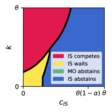
(a) Equilibrium characterization

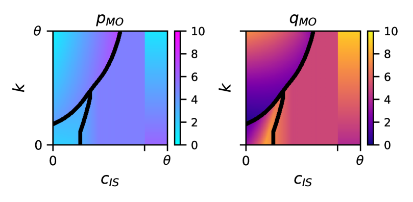
(b) $\mathtt{MO}$’s equilibrium strategies

Figure 13: Equilibrium characterization and $\mathtt{MO}$’s corresponding strategies for different combinations of $k$ and $c_{\mathtt{IS}}$ under proportional rationing. The other game parameters are fixed at $c_{\mathtt{MO}}=2$ and $\alpha=0.2$.

Appendix E Plots and Proofs for Section 5

Figure 14 illustrates the consumer surplus under intensity rationing for different cases, assuming that $\mathtt{IS}$ fully meets demand at the price they set. This provides intuition for the $\mathrm{CS}$ formula in Section 5.

(a) CS for $p_{\mathtt{IS}}\leq p_{\mathtt{MO}}$ and any rationing rule

(b) CS for $p_{\mathtt{IS}}\geq q_{\mathtt{MO}}$ and intensity rationing

Figure 14: A visualization of consumer surplus under the assumption that $q_{\mathtt{IS}}=D_{\mathtt{IS}}$. Blue denotes consumer surplus due to $\mathtt{IS}$’s sales. Green denotes consumer surplus due to $\mathtt{MO}$’s sales.

Proof of Proposition 3.

We break this into three cases.

Case 1: $p_{\mathtt{MO}}\geq p^{\star}_{\mathtt{IS}}$. This is effectively the same as if the marketplace operator were not participating because the independent seller will simply set $p_{\mathtt{IS}}=p^{\star}_{\mathtt{IS}}$ as they would have had the marketplace operator not been a seller (Proposition 3). Thus, the consumer surplus with the marketplace operator is equal to without.

Case 2: $p_{\mathtt{MO}}<p^{\star}_{\mathtt{IS}}$ and the independent seller abstains. By Proposition 5, we know that under intensity rationing, the independent seller abstains only if $q_{\mathtt{MO}}\geq\theta-p_{0}(\geq Q(p^{\star}_{\mathtt{IS}}))$. Thus, we can be in this case only if $\mathtt{MO}$ has offered more inventory compared to when $\mathtt{IS}$ is the sole seller and at a lower price. In other words, $p_{\mathtt{MO}}<p^{\star}_{\mathtt{IS}}$ and $q_{\mathtt{MO}}\geq Q(p^{\star}_{\mathtt{IS}})$, which implies the consumer surplus must be larger than $\mathrm{CS}^{\star}$.

Case 3: $p_{\mathtt{MO}}<p^{\star}_{\mathtt{IS}}$ and the independent seller competes or waits. By Propositions 4 and 5, we know that under intensity rationing, the independent seller will set $p_{\mathtt{IS}}\leq p_{\mathtt{MO}}(<p^{\star}_{\mathtt{IS}})$ whenever they are not abstaining. Furthermore, by Proposition 2, we know that the independent seller will fully meet demand, so the effect is that there is more total inventory at a lower price. This necessarily increases the consumer surplus. We visualize this in Figure 15, which shows that regardless of whether $\mathtt{IS}$ waits or competes, the CS when $\mathtt{MO}$ is a seller (represented by the striped orange and magenta regions) is always larger than $\mathrm{CS}^{\star}$ (represented by the solid blue triangle). ∎

(a) $\mathtt{IS}$ waits

(b) $\mathtt{IS}$ competes

Figure 15: Blue denotes the consumer surplus when the independent seller is the sole seller. The striped regions denote consumer surplus when the marketplace operator is also a seller, where the orange and magenta denote consumer surplus due to the operator’s and independent seller’s sales, respectively.

Figure 16 recreates the rightmost plot in Figure 9 for 36 different $(k,\alpha)$ combinations. We observe that, regardless of the value of the game parameters, the welfare in Game 2 is always at least a high, and is often higher, than the welfare when $\mathtt{IS}$ is the only seller.

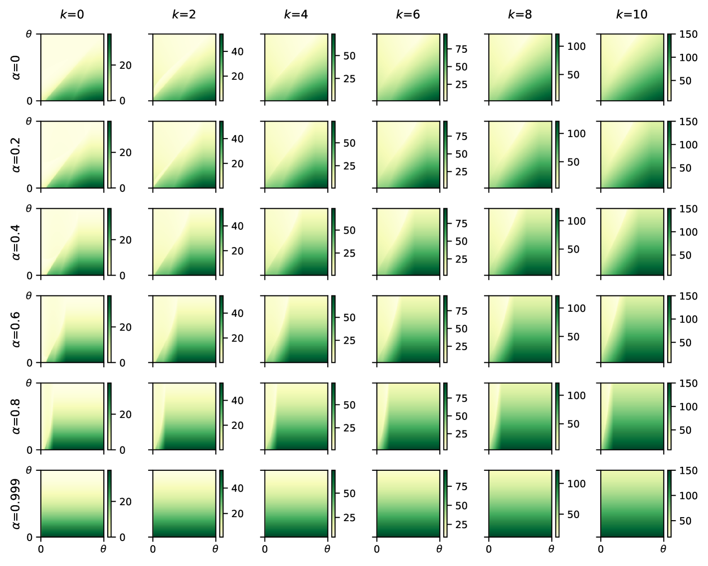
Figure 16: Difference in the equilibrium welfare of Game 2 and the welfare when $\mathtt{IS}$ is the only seller for different combinations of game parameters. Each individual plot varies over $c_{\mathtt{IS}}$ on the x-axis and $c_{\mathtt{MO}}$ on the y-axis. Each row of plots corresponds to a value of $\alpha\in\{0,0.2,0.4,0.6,0.8,0.999\}$ and each column corresponds to a value of $k\in\{0,2,4,6,8,10\}$. We use $\alpha=0.999$ rather than $\alpha=1$ in the bottom row because the “$\mathtt{IS}$ only" game is not well-defined when $\alpha=1$ because this would mean $\mathtt{IS}$ must pay 100% of their revenue to $\mathtt{MO}$. The minimum and maximum values of each colorbar correspond to the minimum and maximum values in the data being displayed.

References

- Armstrong (2006) Mark Armstrong. Competition in two-sided markets. The RAND Journal of Economics, 37(3):668–691, 2006.
- Banerjee et al. (2017) Siddhartha Banerjee, Sreenivas Gollapudi, Kostas Kollias, and Kamesh Munagala. Segmenting two-sided markets. In Proceedings of the 26th International Conference on World Wide Web, pages 63–72, 2017.
- Bertrand (1883) Joseph Bertrand. Review of “theorie mathematique de la richesse sociale” and of “recherches sur les principles mathematiques de la theorie des richesses.”. Journal Des Savants, 67:499, 1883.
- Birge et al. (2021) John Birge, Ozan Candogan, Hongfan Chen, and Daniela Saban. Optimal commissions and subscriptions in networked markets. Manufacturing & Service Operations Management, 23(3):569–588, 2021.
- Boyer and Moreaux (1987) Marcel Boyer and Michel Moreaux. Being a leader or a follower: Reflections on the distribution of roles in duopoly. International Journal of Industrial Organization, 5(2):175–192, 1987.
- Boyer and Moreaux (1989) Marcel Boyer and Michel Moreaux. Endogenous rationing in a differentiated product duopoly. International Economic Review, pages 877–888, 1989.
- Caillaud and Jullien (2003) Bernard Caillaud and Bruno Jullien. Chicken & egg: Competition among intermediation service providers. RAND Journal of Economics, pages 309–328, 2003.
- Cournot (1897) Augustin Cournot. Researches Into the Mathematical Principles of the Theory of Wealth. Macmillan, 1897.
- Cremer et al. (1989) Helmuth Cremer, Maurice Marchand, and Jacques-Francois Thisse. The public firm as an instrument for regulating an oligopolistic market. Oxford Economic Papers, 41(1):283–301, 1989.
- D’Amico-Wong et al. (2024) Luca D’Amico-Wong, Yannai A. Gonczarowski, Gary Qiurui Ma, and David C Parkes. Disrupting bipartite trading networks: Matching for revenue maximization. arXiv preprint arXiv:2406.07385, 2024.
- Davidson and Deneckere (1986) Carl Davidson and Raymond Deneckere. Long-run competition in capacity, short-run competition in price, and the Cournot model. The RAND Journal of Economics, pages 404–415, 1986.
- De Fraja and Delbono (1990) Giovanni De Fraja and Flavio Delbono. Game theoretic models of mixed oligopoly. Journal of Economic Surveys, 4(1):1–17, 1990.
- Eden et al. (2023) Alon Eden, Gary Qiurui Ma, and David C Parkes. Platform equilibrium: Analayzing social welfare in online market places. arXiv preprint arXiv:2309.08781, 2023.
- Edgeworth (1925) Francis Ysidro Edgeworth. The pure theory of monopoly. Papers Relating to Political Economy, 1:111–142, 1925.
- Kreps and Scheinkman (1983) David M. Kreps and Jose A. Scheinkman. Quantity precommitment and Bertrand competition yield Cournot outcomes. The Bell Journal of Economics, pages 326–337, 1983.
- Levitan and Shubik (1978) Richard Levitan and Martin Shubik. Duopoly with price and quantity as strategic variables. International Journal of Game Theory, 7:1–11, 1978.
- Maskin and Tirole (1988) Eric Maskin and Jean Tirole. A theory of dynamic oligopoly, II: Price competition, kinked demand curves, and Edgeworth cycles. Econometrica: Journal of the Econometric Society, pages 571–599, 1988.
- Molina (2021) Brett Molina. iPhone 13: Yes, people still wait in line to get the new iPhone. https://www.yahoo.com/tech/iphone-13-yes-people-still-141554786.html, 2021. Accessed: 28 December 2024.
- Nakamura and Inoue (2009) Yasuhiko Nakamura and Tomohiro Inoue. Endogenous timing in a mixed duopoly: Price competition with managerial delegation. Managerial and Decision Economics, 30(5):325–333, 2009.
- Pabari et al. (2025) Raj Pabari, Udaya Ghai, Dominique Perrault-Joncas, Kari Torkkola, Orit Ronen, Dhruv Madeka, Dean Foster, and Omer Gottesman. A shared-revenue Bertrand game. arXiv preprint arXiv:2502.07952, 2025.
- Pal (1998) Debashis Pal. Endogenous timing in a mixed oligopoly. Economics Letters, 61(2):181–185, 1998.
- Rasmusen (1989) Eric Rasmusen. Games and Information. Basil Blackwell Oxford, 1989.
- Rochet and Tirole (2003) Jean-Charles Rochet and Jean Tirole. Platform competition in two-sided markets. Journal of the European Economic Association, 1(4):990–1029, 2003.
- Shopova (2023) Radostina Shopova. Private labels in marketplaces. International Journal of Industrial Organization, 89:102949, 2023.
- Shubik (1959) Martin Shubik. Strategy and Market Structure: Competition, Oligopoly, and the Theory of Games. Wiley, 1959. ISBN 9780598679451.
- Stackelberg (1934) Heinrich von Stackelberg. Marktform und gleichgewicht. 1934.
- Tirole (1988) Jean Tirole. The Theory of Industrial Organization. MIT Press, 1988.
- Vives (1999) Xaview Vives. Oligopoly Pricing: Old Ideas and New Tools. MIT Press, 1999.
- Vohra and Krishnamurthi (2012) Rakesh V. Vohra and Lakshman Krishnamurthi. Principles of Pricing: an Analytical Approach. Cambridge University Press, 2012.
- Yousefimanesh et al. (2023) Niloofar Yousefimanesh, Iwan Bos, and Dries Vermeulen. Strategic rationing in Stackelberg games. Games and Economic Behavior, 140:529–555, 2023.