Triple Higgs Production at Muon Colliders in the Higgs Triplet Model

Abstract

The production of three Higgs bosons provides a unique opportunity to probe both the trilinear and quartic Higgs couplings within the Standard Model and beyond. In this study, we investigate triple Higgs production in the Higgs Triplet Model via photon fusion, $\gamma\gamma\to h^{0}h^{0}h^{0}$, allowing us to explore the contributions from singly and doubly charged Higgs bosons and their couplings to CP-even scalars. We analyze the total cross sections and kinematic distributions, comparing our results with the corresponding SM predictions. Our calculations utilize an Automated One-Loop Calculator to evaluate the numerical amplitudes for the $2\to 3$ process. For the collider simulations, we develop a Monte Carlo phase-space integrator to predict outcomes for a future muon collider, covering a center-of-mass energy range from 2 TeV to 10 TeV.

I Introduction

In the Standard Model (SM), the scalar potential of the Higgs sector is given by

$$V_{SM}\supset\frac{M_{h}^{2}}{2}h^{2}+\frac{1}{3!}\frac{3M_{h}^{2}}{v}h^{3}+\frac{1}{4!}\frac{3M_{h}^{2}}{v^{2}}h^{4}.$$ (1)

Here, $h$ represents the physical Higgs field, $v$ represents the vacuum expectation value, and $M_{h}$ is the Higgs boson mass. In this framework, the trilinear Higgs coupling and quartic Higgs coupling are expressed as $\lambda_{hhh}=\frac{3M_{h}^{2}}{v}$ and $\lambda_{hhhh}=\frac{3M_{h}^{2}}{v^{2}}$ [1]. Any deviations from these SM predictions suggest the presence of physics beyond the SM. Precise measurements of these couplings provide a valuable approach for probing new physics and unraveling the structure of the Higgs potential, which plays a crucial role in electroweak symmetry breaking [2, 3, 4, 5]. Additionally, exploring the Higgs potential in detail is key to understanding the mechanisms underlying the electroweak phase transition and the matter-antimatter asymmetry in the universe, [6, 7, 8].

The process of producing three Higgs bosons offers a unique avenue to directly study the Higgs self-coupling. While double Higgs production provides insight into the trilinear Higgs coupling [9, 10, 11, 12, 13], triple Higgs production goes a step further by probing the quartic Higgs self-coupling. The quartic self-coupling is an essential component of the Higgs potential [14]. Despite its importance, this aspect of the potential remains experimentally unexplored, highlighting the need for further investigation into the fundamental properties of the Higgs boson [15].

In proton colliders, the dominant production mechanisms for double Higgs ($hh$) and triple Higgs ($hhh$) processes occur via gluon fusion. At a center-of-mass energy of $\sqrt{s}=14~\mathrm{TeV}$, the cross section for $hh$ production is approximately 300 times larger than that for $hhh$ production. At next-to-next-to-leading order (NNLO), the cross sections are given by $\sigma(hh)=36.69\pm 3.0\%~{\rm fb}\quad\text{and}\quad\sigma(hhh)=0.103\pm 15\%~{\rm fb}$ [16, 17, 18, 11, 2].

The production of three Higgs bosons at the LHC is currently beyond the detection threshold due to its extremely low cross section. This, coupled with significant background noise and the LHC’s limited integrated luminosity, makes it nearly impossible to observe a sufficient number of $hhh$ events for robust analysis [19, 20, 21, 3]. Even at a center-of-mass energy of $\sqrt{s}=14~\mathrm{TeV}$, the process remains highly suppressed. Future collider projects, Ref. [22, 23] with increased energy and luminosity, such as a Future Circular Collider (FCC) [24, 25] would be necessary to achieve meaningful sensitivity to triple Higgs production [26, 27].

In a muon collider [28, 29, 30] the collision of high-energy muon beams can result in the emission of two collinear photons. These photons may interact to produce multiple Higgs bosons, including triple Higgs boson production. This process is facilitated by a loop-induced mechanism, where virtual particles such as heavy fermions and gauge bosons mediate the effective coupling between the photons and Higgs bosons [31, 32, 33]. The photon-photon interaction in this scenario can significantly enhance the effective cross-section for triple Higgs production, making it a rare yet important process to study [34, 35]. Moreover, the muon collider’s clean experimental environment and high luminosity provide a unique opportunity to examine the Higgs boson self-couplings and explore the structure of the Higgs potential in greater detail, [36, 37, 38, 39, 40, 41, 42].

In scenarios extending Beyond the Standard Model (BSM), the production of multiple Higgs bosons [43, 44, 27, 45, 46, 47, 48] such as three Higgs bosons, can be substantially enhanced due to the presence of new particles and interactions that modify the Higgs sector. BSM frameworks, including the Higgs Triplet Model (HTM) [49], and Two-Higgs Doublet Models (2HDM) [50, 51, 52], introduce additional scalar fields, such as charged Higgs bosons, which contribute to higher production rates compared to the SM predictions. Moreover, these models may predict the existence of Higgs-like particles absent in the SM, providing a window into the structure of an extended Higgs sector. For example, the HTM allows for the production of three charged Higgs bosons, enabling the study of new couplings derived from the extended scalar potential, thereby distinguishing these models from the SM. A detailed analysis of three Higgs production via photon fusion and VBF processes in the SM context is presented in Ref. [32]. Investigations into triple Higgs production also reveal insights into the complex mechanisms of electroweak symmetry breaking [53] in BSM theories, helping differentiate among various extensions. A comprehensive study on the production of three Higgs bosons within the framework of the Two Real Singlet Extension Model is presented in Ref. [54].

In 2012, the ATLAS and CMS collaborations announced the discovery of the Higgs boson, with its mass measured at $125.6\pm 0.3\,{\rm GeV}$ [55, 56]. While this result aligns closely with the predictions of the SM, it is important to explore scenarios beyond the SM that could influence Higgs decay channels and self-couplings [57]. The SM assumes neutrinos are massless, as there are no right-handed neutrinos to generate a Dirac mass term. However, measurements from experiments like MAINZ, [58, 59], TROITSK [60, 61], and KATRIN [62, 63, 64], suggest the need for a new mass scale in the neutrino sector.

There are various models for generating neutrino mass, including the addition of right-handed neutrinos or mechanisms such as the inverse seesaw. Our work focuses on the Type II Seesaw mechanism. The core idea of the seesaw mechanism is to introduce additional fields that couple to the SM fermions, with a mass scale significantly higher than the electroweak scale. In the HTM (Type II seesaw model), left-handed lepton doublets are couple to a triplet field, leading to neutrino masses proportional to the Yukawa coupling and the vacuum expectation value of the triplet [65, 66].

This paper is organized as follows: Sections II and III provides an overview of the HTM and introduces the parameter scanning methodology. Section IV details the calculations and the Monte Carlo methods used. In Section V, we present and analyze the results. Finally, Section VI concludes the paper, summarizing our findings.

II The Higgs Triplet Model

To generate mass for neutrinos, the SM, which includes a Higgs doublet $\Phi\sim(1,2,1/2)$, is extended by incorporating a $SU(2)_{L}$ Higgs triplet field $\Delta$. This extension allows for the creation of a Yukawa coupling between the SM leptons and the new scalar fields, which is expressed as follows:

$$\mathcal{L}\supset Y_{ij}L_{i}^{T}C\otimes i\sigma_{2}\Delta L_{j}+h.c.$$ (2)

Here, $L_{i}$ and $L_{j}$ denote the left-handed lepton doublets, $C$ is the charge conjugation operator, $\sigma_{m}$, ($m=1,2,3$), represents the Pauli matrices, and $Y_{ij}$ corresponds to the Yukawa coupling associated with the neutrino sector, which is an element of a complex symmetric matrix. The indices $i$ and $j$ refer to the lepton flavors $e$, $\mu$, and $\tau$ [67, 68, 69, 70, 71, 72, 73, 74, 75].

The doublet field, which has a weak hypercharge of $Y_{\Phi}=1$, and the triplet field $\Delta$, represented in a $2\times 2$ matrix form with a weak hypercharge of $Y_{\Delta}=2$, are defined as follows:

$$\Phi=\begin{pmatrix}\phi^{+}\\ \phi^{0}\end{pmatrix},\quad\Delta=\begin{pmatrix}\frac{\delta^{+}}{\sqrt{2}}&\delta^{++}\\ \delta^{0}&-\frac{\delta^{+}}{\sqrt{2}}\end{pmatrix}.$$

The triplet Higgs field $\Delta$ acquires a small vacuum expectation value (VEV), $v_{\Delta}$, which plays a crucial role in generating neutrino masses through the Type II Seesaw mechanism. After electroweak symmetry breaking, the neutrino mass matrix is given by $m_{\nu}=Y_{\nu}v_{\Delta}$. The smallness of neutrino masses is naturally explained by the tiny value of $v_{\Delta}$, which is typically on the order of $\mathcal{O}(1)$ eV, ensuring consistency with experimental observations of neutrino mass scales [71, 73].

The scalar sector, including the kinetic terms and potential for $\Phi$ and $\Delta$, is given by:

$$\mathcal{L}_{s}=(D_{\mu}\Phi)^{\dagger}(D^{\mu}\Phi)+\text{Tr}[(D_{\mu}\Delta)^{\dagger}(D^{\mu}\Delta)]-V(\Phi,\Delta),$$ (3)

where the covariant derivatives,

$$D_{\mu}\Phi=\partial_{\mu}\Phi+i\frac{g}{2}\sigma^{m}W^{m}_{\mu}\Phi+i\frac{g^{{}^{\prime}}}{2}B_{\mu}\Phi,$$ (4)

and,

$$D_{\mu}\Delta=\partial_{\mu}\Delta+ig[\frac{1}{2}\sigma^{m}W^{m}_{\mu},\Delta]+i\frac{g^{{}^{\prime}}}{2}Y_{\Delta}B_{\mu}\Delta,$$ (5)

are defined with the $SU(2)$ and $U(1)$ gauge field couplings, $g$ and $g^{\prime}$, respectively. The general renormalizable potential term is introduced as [73]:

$$V(\Phi,\Delta) = -\mu_{\Phi}^{2}\Phi^{\dagger}\Phi+\frac{\lambda}{4}(\Phi^{\dagger}\Phi)^{2}+\mu^{2}_{\Delta}Tr(\Delta^{\dagger}\Delta)$$

$$+ [\mu(\Phi^{T}i\sigma^{2}\Delta^{\dagger}\Phi)+h.c]+\lambda_{1}(\Phi^{\dagger}\Phi)Tr(\Delta^{\dagger}\Delta)$$

$$+ \lambda_{2}(Tr\Delta^{\dagger}\Delta)^{2}+\lambda_{3}Tr(\Delta^{\dagger}\Delta)^{2}+\lambda_{4}\Phi^{\dagger}\Delta\Delta^{\dagger}\Phi.$$

The scalar potential in the HTM involves several parameters with distinct roles and dimensions. The mass parameters include $\mu_{\Phi}^{2}<0$, which has dimensions of $[\text{mass}^{2}]$ and determines the mass term for the SM Higgs doublet $\Phi$. A negative value for $\mu_{\Phi}^{2}$ ensures spontaneous symmetry breaking, leading to the generation of the Higgs VEV, $v_{\Phi}$. Similarly, $\mu_{\Delta}^{2}$, also with dimensions of $[\text{mass}^{2}]$, controls the mass term for the Higgs triplet $\Delta$. A positive value for $\mu_{\Delta}^{2}$ ensures that the triplet does not acquire a large VEV, $v_{\Delta}=\mu^{2}v^{2}/(2\mu_{\Phi}^{2})$. Additionally, the dimensionful parameter $\mu$, with dimensions of $[\text{mass}]$, couples the doublet $\Phi$ to the triplet $\Delta$ and plays a critical role in generating a small vacuum expectation value for $\Delta$ through the Type II Seesaw mechanism [76]. The minimization of the Higgs potential in the HTM is essential for ensuring the correct pattern of electroweak symmetry breaking. By minimizing the potential, one obtain the following conditions that relate the parameters of the model to the VEVs:

$$\mu_{\Phi}^{2}=\frac{\lambda v^{2}_{\Phi}}{4}-\sqrt{2}\mu v_{\Delta}+\frac{(\lambda_{1}+\lambda_{4})v_{\Delta}}{2}$$ (7)

and,

$$\mu_{\Delta}^{2}=\frac{2\mu v^{2}_{\phi}-\sqrt{2}(\lambda_{1}+\lambda_{4})v_{\Phi}^{2}v_{\Delta}-2\sqrt{2}(\lambda_{2}+\lambda_{3})v_{\Delta}^{3}}{2\sqrt{2}v_{\Delta}}.$$ (8)

The dependence of $\mu_{\Phi}^{2}$ and $\mu_{\Delta}^{2}$ on the $\lambda_{i}$ couplings is also important because these Lagrangian parameters modify the couplings of the Higgs boson to gauge bosons and fermions, which can be investigated at collider experiments.

In HTM, the Higgs sector includes a doublet and a triplet, resulting in 10 real scalar degrees of freedom before EWSB. After EWSB, three Goldstone bosons are absorbed by the $W^{\pm}$ and $Z^{0}$ bosons, leaving seven physical Higgs states: two CP-even neutral Higgs bosons $h^{0}$ and $H^{0}$, one CP-odd neutral Higgs boson $A^{0}$, one singly charged Higgs $H^{\pm}$, and one doubly charged Higgs $H^{\pm\pm}$ [68].

The mixing between these states is determined by three mixing angles: $\alpha$ for the CP-even Higgses, $\beta$ for the CP-odd Higgses, and $\beta^{{}^{\prime}}$ for the charged Higgses. These mixings arise from the interactions between the Higgs doublet and triplet components, affecting the phenomenology and collider signatures of the Higgs sector [66].

$$h^{0}=h\cos{\alpha}+\xi\sin{\alpha}.$$ (9)

$$H^{0}=-h\sin{\alpha}+\xi\cos{\alpha}.$$ (10)

Here, $h=\text{Re}[\phi^{0}]$ and $\xi=\text{Re}[\delta^{0}]$ are shifted by their VEVs. The triplet VEV ($v_{\Delta}$) is crucial in determining the strength of these mixings, influencing the production and decay channels of the extended Higgs sector in the Type-II Seesaw Model [77].

Probing quartic and trilinear scalar couplings in the HTM provides an opportunity to examine the shape of the Higgs potential by reparameterizing $\mu_{\Delta}$ and $\mu_{\Phi}$ in terms of $\lambda$, $\lambda_{i}$ (where $i\in{1,2,3,4}$), and $\mu$. To establish a parameter space for collider simulations, we propose the following input set, noting that $v=\sqrt{v_{\Phi}^{2}+2v_{\Delta}^{2}}=246~\mathrm{GeV}$:

$$\mathcal{P}_{1}=\{M_{h^{0}},M_{H^{0}},M_{A^{0}},M_{H^{\pm}},M_{H^{\pm\pm}},v_{\Delta},\cos{\alpha}\}.$$ (11)

To establish a well-reasoned selection of parameters within the framework of the HTM, one must consider the $\rho$-parameter, the mass splitting between charged Higgs bosons, perturbativity, and vacuum stability. The $\rho$-parameter, given by

$$\rho=\frac{1+2v^{2}_{\Delta}/v_{\Phi}^{2}}{1+4v^{2}_{\Delta}/v_{\Phi}},$$ (12)

places an upper limit on $v_{\Delta}$ of approximately 8 GeV to ensure that the experimental value of the $\rho$-parameter remains close to unity [78].

The mass splitting between $H^{\pm}$ and $H^{\pm\pm}$, constrained by electroweak precision data, implies that $|\Delta M|<50$ [79]. The mass hierarchy of the charged Higgs bosons depends on the sign of $\Delta M$.

To guarantee vacuum stability, ensuring that the scalar potential $V(\Phi,\Delta)$ remains bounded from below and does not enter an instability regime, the parameters in the scalar potential must satisfy the following conditions:

$$\lambda\geq 0;~\lambda_{2}+\lambda_{3}\geq 0;~\lambda_{2}+\frac{\lambda_{3}}{2}\geq 0\ ,$$ (13)

$$\lambda_{1}+\sqrt{\lambda(\lambda_{2}+\lambda_{3})}\geq 0;~\lambda_{1}+\sqrt{\lambda(\lambda_{2}+\frac{\lambda_{3}}{2})}\geq 0$$ (14)

and,

$$\lambda_{1}+\lambda_{4}+\sqrt{\lambda(\lambda_{2}+\lambda_{3})}\geq 0;~\lambda_{1}+\lambda_{4}+\sqrt{\lambda(\lambda_{2}+\frac{\lambda_{3}}{2})}\geq 0\ .$$ (15)

Additionally, we have imposed the constraint $|\lambda_{i}|\leq 4\pi$ to maintain perturbativity [68]. A detailed discussion on perturbativity and vacuum stability can be found in Ref. [67, 71].

III Framework for Parameter Space Investigation

When studying SM-like Higgs production and decay processes in the HTM or other extended Higgs scalar models, selecting the input parameters efficiently and consistently is essential for ensuring theoretical and phenomenological accuracy. The masses of the Higgs scalars and the mixing angle $\alpha$ are physical parameters that inherently depend on the scalar potential parameters ($\lambda_{i}$, $\lambda$, $\mu$). To evaluate the scalar potential parameters, one can use the following expressions [15, 80, 67]:

$$\lambda=-\frac{2}{v_{\Phi}^{2}}(c_{\alpha}^{2}M^{2}_{h}+s^{2}_{\alpha}M^{2}_{H})\ ,$$ (16)

$$\lambda_{1}=-\frac{2}{v_{\Phi}^{2}+4v^{2}_{\Delta}}M_{A}^{2}+\frac{2}{v_{\Phi}^{2}+2v^{2}_{\Delta}}M_{H^{\pm}}^{2}$$ (17)

$$-\frac{\sin{2\alpha}}{2v_{\Delta}v_{\Phi}}(M_{H}^{2}-M_{h}^{2})\ ,$$

$$\lambda_{2}=\frac{1}{2v_{\Delta}^{2}}\Big{(}c_{\alpha}^{2}M^{2}_{h}+s^{2}_{\alpha}M^{2}_{H}+\frac{v^{2}_{\Delta}}{v_{\Phi}^{2}+4v^{2}_{\Delta}}M_{A}^{2}-$$ (18)

$$\frac{4v^{2}_{\Delta}}{v_{\Phi}^{2}+2v^{2}_{\Delta}}M_{A}^{2}+2M^{2}_{H^{\pm\pm}}\Big{)}\ ,$$

$$\lambda_{3}=\frac{1}{v_{\Delta}^{2}}\Big{(}-\frac{v^{2}_{\Phi}}{v_{\Phi}^{2}+4v^{2}_{\Delta}}M_{A}^{2}+\frac{2v^{2}_{\Phi}}{v_{\Phi}^{2}+2v^{2}_{\Delta}}M^{2}_{H^{\pm}}-M^{2}_{H^{\pm\pm}}\Big{)}\ ,$$ (19)

$$\lambda_{4}=\frac{4}{v_{\Phi}^{2}+4v^{2}_{\Delta}}M_{A}^{2}-\frac{4}{v_{\Phi}^{2}+2v^{2}_{\Delta}}M^{2}_{H^{\pm}}\ ,$$ (20)

$$\mu=\frac{\sqrt{2}v_{\Phi}}{v_{\Phi}^{2}+4v^{2}_{\Delta}}M^{2}_{A}\ .$$ (21)

The masses of the Higgs bosons are directly related to observable quantities measurable in collider experiments. Utilizing $\mathcal{P}_{1}$ space, Eq. 11, ensures that simulations remain consistent with experimental constraints. The choice of $\alpha$ is critical in determining the degree of mixing between the doublet-like and triplet-like states, ensuring consistency with current experimental data and precise Higgs coupling measurements [72]. However, during simulations, calculating $\lambda_{i}$, $\lambda$, $\mu$ from $\mathcal{P}_{1}$ can be computationally challenging, especially when considering the mass splittings between the charged Higgs bosons and the neutral Higgs bosons. Therefore, this highlights the need to develop a reliable method for deducing the parameter functions from the mass values in $\mathcal{P}_{1}$. However, this is demanding due to the high sensitivity of $\lambda_{2}$ and $\lambda_{3}$, particularly when ensuring compliance with vacuum stability and perturbativity constraints.

If one calculates $\lambda_{2}$ and $\lambda_{3}$ using the parameters in $\mathcal{P}_{1}$ and Eqs. 20-21, and then introduces a minute adjustment, ($\sim 10^{-4}~\mathrm{GeV}$), to the scalar masses, $\delta M_{A^{0},H^{0},H^{\pm},H^{\pm\pm}}$, the values of $\lambda_{2}$ and $\lambda_{3}$ can increase significantly. If these parameters become excessively large, the contributions from $s$-channel scalar exchange to Drell-Yan processes would dominate, [81, 49, 15], potentially leading to incorrect tree-level results. As discussed in Ref. [81, 15], this pronounced sensitivity represents a theoretical issue rather than merely a numerical challenge. This behavior, which can be described as highly reactive, is not always a direct consequence of variations in $\delta M_{A^{0},H^{0},H^{\pm},H^{\pm\pm}}/v_{\Delta}$. Instead, it can arise purely from inconsistencies in the mass parameters, particularly when evaluated at $v_{\Delta}=1\,\mathrm{GeV}$. These inconsistencies emphasize the necessity for precise parameter tuning to maintain theoretical consistency and prevent inaccurate results in cross sections and kinematic distributions.

To develop an effective approach for parameter scanning, we begin by ensuring that the square root terms in Eqs. (14) and (15) remain real. This requirement imposes the conditions that both $\lambda_{2}+\lambda_{3}$ and $\lambda_{2}+\lambda_{3}/2$ must be positive [80]. These scenarios form the basis for deriving the resultant expressions in Eqs. 22 and 23, which are then used to deduce the masses of the singly charged Higgs boson and the pseudoscalar. The approach relies on input parameters including $M_{H^{\pm\pm}}$, $M_{H^{0}}$, $M_{h^{0}}$, $\cos{\alpha}$, and $v_{\Delta}$. By carefully selecting these inputs, the method ensures consistency between theoretical predictions and experimental constraints, providing a sufficient and robust framework for exploring the parameter space of the model.

$$M_{A^{0}}^{\text{max}}=\frac{(v^{2}_{\Phi}+4v_{\Delta}^{2})^{1/2}}{v_{\Phi}}(\cos{\alpha}^{2}M_{H^{0}}^{2}+\sin{\alpha}^{2}M_{h^{0}}^{2})^{1/2}\ ,$$ (22)

$$M_{H^{\pm}}^{\text{max}}=\frac{(v^{2}_{\Phi}+2v_{\Delta}^{2})^{1/2}}{\sqrt{2}v_{\Phi}}(M^{2}_{H^{\pm\pm}}+\cos{\alpha}^{2}M_{H^{0}}^{2}+\sin{\alpha}^{2}M_{h^{0}}^{2})^{1/2},$$ (23)

When selecting numerical inputs for the mass of the singly charged Higgs boson, based on the masses of the heavy Higgs and the doubly charged Higgs as per Eq. 23, one can determine it as:

$$M_{H^{\pm}}=M_{H^{\pm}}^{\text{max}}\pm\delta M_{H^{\pm}}.$$ (24)

The Eqs. 22 and 23 highlight that the singly charged Higgs boson and the pseudoscalar boson have maximum values they can attain within the parameter space $\mathcal{P}_{2}=\mathcal{P}_{1}\setminus\{M_{H^{\pm}},M_{A^{0}}\}$, which serves as a sufficient condition for stability. If one chooses $M_{H^{\pm}}$ such that $M_{H^{\pm}}\lessgtr M_{H^{\pm}}^{\text{max}}$, it could lead to either a violation of vacuum stability or a breakdown of perturbativity, particularly for sufficiently large variations $\epsilon=\delta M_{H^{\pm}}$. This emphasizes the need for careful parameter selection to maintain theoretical consistency, see the Fig. 1. For sufficiently large values of $\epsilon$, $M^{\text{max}}_{H^{\pm}}+\epsilon$ can result in a violation of vacuum stability. Similarly, for certain values of $\epsilon$, $M^{\text{max}}_{H^{\pm}}-\epsilon$ may lead to a breakdown of perturbativity.

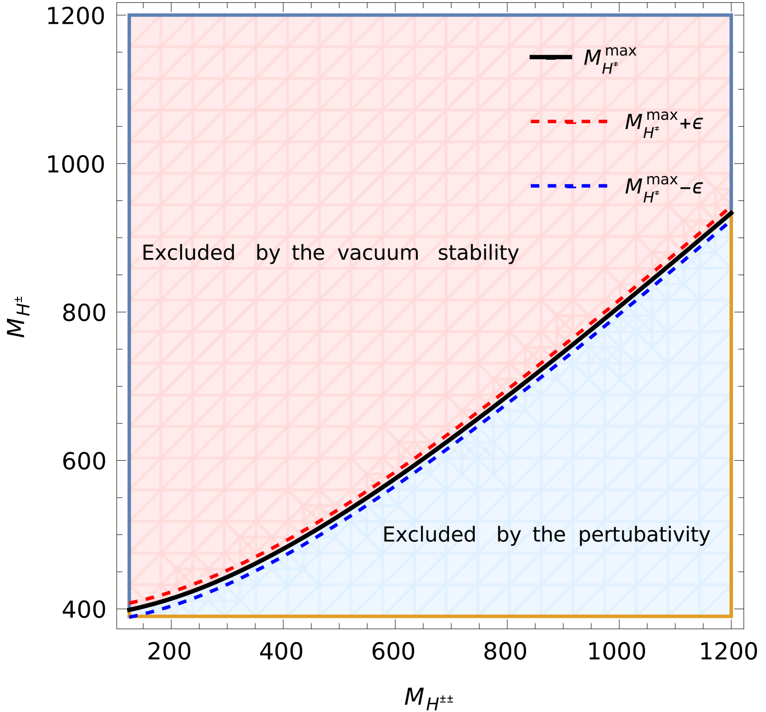
Figure 1: The mass of $H^{\pm}$ as a function of $M_{H^{\pm\pm}}$, with $M_{H^{0}}=600~\mathrm{GeV}$, $v_{\Delta}=1$, and $\cos{\alpha}=0.9999$. For any value chosen above the red dashed lines, the potential term becomes unstable, and for values below the blue dashed lines, the parameter functions of the potential violate perturbativity.

Now, let us express $\lambda_{2,3}$ as functions of the parameters in the space $\mathcal{P}_{2}\cup\{M_{H^{\pm}}^{\text{max}}-\epsilon,M_{A^{0}}^{\text{max}}\}$. The corresponding results, denoted as $\tilde{\lambda}_{2}$ and $\tilde{\lambda}_{2}$, are given by

$$\tilde{\lambda}_{2}=\lambda_{2}+N\epsilon M_{H^{\pm}}~,$$ (25)

and

$$\tilde{\lambda}_{3}=\lambda_{3}-N\epsilon M_{H^{\pm}}~,$$ (26)

with

$$N=\frac{4v_{\Phi}^{2}}{v_{\Delta}^{2}(v_{\Phi}^{2}+2v_{\Delta}^{2})}~.$$ (27)

This indicates that, for certain nonzero values of $|\epsilon|$, the inequalities $|\lambda_{2,3}|\leq 4\pi$ is still hold. This implies that for fixed values of the parameters in $\mathcal{P}_{2}$, there exists an $\epsilon>0$ such that $|\lambda_{3}(M_{H^{\pm}}^{\text{max}}-\epsilon)|\geq 4\pi$ and $|\lambda_{2}(M_{H^{\pm}}^{\text{max}}+\epsilon)|\geq 4\pi$. Moreover, there exists a $\epsilon_{P}\in(0,\epsilon)$ such that $|\lambda_{3}(M_{H^{\pm}}^{\text{max}}-\epsilon_{P})|\leq 4\pi$ and $|\lambda_{2}(M_{H^{\pm}}^{\text{max}}+\epsilon_{P})|\leq 4\pi$. When $\epsilon_{P}<\epsilon$, $\lambda_{2}$ and $\lambda_{3}$ are nonzero and satisfy the conditions for perturbativity. However, when $\epsilon=\epsilon_{P}=0$, $\lambda_{2}$ and $\lambda_{3}$ approach extremely small values. For nonzero values of $\lambda_{2}$ and $\lambda_{3}$, these parameters have a considerable impact on the couplings $\lambda_{H^{0}H^{+}H^{-}}$ and $\lambda_{H^{0}H^{++}H^{--}}$. Although their contributions to $\lambda_{h^{0}H^{+}H^{-}}$ and $\lambda_{h^{0}H^{++}H^{--}}$ couplings are negligible in the limit $\alpha\to 0$, they still play a significant role in the scattering amplitude for the processes $\gamma\gamma\rightarrow h^{0}h^{0},h^{0}h^{0}h^{0}$. By solving the last two inequalities in this section for $\epsilon_{P}$, we find that:

$$\epsilon_{P}=2\sqrt{2}\pi v\frac{v^{2}_{\Delta}}{v_{\Phi}}\frac{1}{\sqrt{M^{2}_{H^{\pm\pm}}+\cos^{2}{\alpha}M_{H0}^{2}+\sin^{2}{\alpha}M_{h^{0}}^{2}}}.$$ (28)

Hence, for all $\epsilon\in\mathbb{R}^{+}\setminus[0,\epsilon_{P}]$, the perturbativity breaks down in the $\mathcal{P}_{1}$ parameter space.

To verify compatibility with the last inequality in the conditions shown in Eq. 15, We consider the modifications introduced by Eq. 23. In the parameter space $\mathcal{P}_{2}\cup\{{M_{H^{\pm}}^{\text{max}}}+\epsilon_{V},M_{A^{0}}^{\text{max}}\}$, assume that there exists a value $\epsilon_{V}>0$ such that the condition $\tilde{\lambda}_{2}+\frac{\tilde{\lambda}_{3}}{2}>0$ is satisfied.

However,

$$\tilde{\lambda}_{2}+\frac{\tilde{\lambda}_{3}}{2}=-\frac{v_{\Phi}^{2}}{2v^{2}_{\Delta}v^{2}}\epsilon_{V}\Big{(}\epsilon_{V}+2M^{\text{max}}_{H^{\pm}}\Big{)},$$ (29)

which implies that $\tilde{\lambda}_{2}+\frac{\tilde{\lambda}_{3}}{2}$ remains positive only if $-2M^{\text{max}}_{H^{\pm}}<\epsilon_{V}<0$.

This results in a contradiction because $\epsilon_{V}$ does not satisfy the positivity condition. Therefore, We can conclude that for every sufficiently large $\epsilon_{V}>0$, the input $M^{\text{max}}_{H^{\pm}}+\epsilon_{V}$ violates the vacuum stability of the Higgs potential.

In the scenario where $\alpha=\pi/4$, the above conditions may not hold, as for non-zero $\alpha$, $\lambda_{1}+\lambda_{4}$ can become negative, potentially could not satisfy $\lambda_{1}+\lambda_{4}>-\sqrt{\lambda(\lambda_{2}+\lambda_{3}/2)}.$ This violates the bounded-from-below condition presented in Eq. 15.

Therefore, without explicitly solving the inequality to derive the scalar mass limits, We deduced sufficient conditions for $\lambda_{1}+\lambda_{4}>0$, which provides an upper bound on the heavy Higgs mass for $\alpha\in(0,\pi/2)$. This inequality consequently leads to a lower bound on the pseudo-scalar mass, expressed as:

$$M^{\text{min}}_{A^{0}}=\frac{1}{2}\sqrt{\frac{v_{\Phi}^{2}+4v_{\Delta}^{2}}{v_{\Delta}v_{\Phi}}}\sqrt{(\Delta M_{s}^{2})\sin{2\alpha}}.$$ (30)

Where $\Delta M_{s}^{2}=M^{2}_{H^{0}}-M_{h^{0}}^{2}$. Now, comparing this with Eq. 22, we find that $M_{A^{0}}^{\text{min}}\leq M_{A^{0}}^{\text{max}}$, which provides:

$$M_{H^{0}}^{\text{max}}=\Big{(}1+\frac{2v_{\Delta}}{v_{\Phi}}\tan{\alpha}\Big{)}^{1/2}\Big{(}1-\frac{2v_{\Delta}}{v_{\Phi}}\frac{1}{\tan{\alpha}}\Big{)}^{-1/2}M_{h^{0}}.$$ (31)

This relationship holds for $\tan{\alpha}>\frac{2v_{\Delta}}{v_{\Phi}}$, and the constraint arising from the $\rho$ parameter bounds $v_{\Delta}<8\,\mathrm{GeV}$ [73].

IV Methodology

In the SM and the HTM, the one-loop processes $\gamma\gamma\rightarrow h^{0}h^{0}h^{0}$ are mediated by triangle, box, self-energy, and pentagon diagrams. In the HTM, these diagrams are sensitive to contributions from fermions, $W^{\pm}$ bosons, and charged Higgs bosons within the loops, as illustrated in Fig. 2. Due to the large number of diagrams, here we display only generic Feynman diagrams for simplicity. If all the contributions mediated by $H^{\pm}$ and $H^{\pm\pm}$ are excluded, the remaining diagrams correspond to the SM case.

To perform these calculations, we begin by using Mathematica and FeynRules [82, 83] to generate the Universal FeynRules Output (UFO) model file for the HTM. The FeynRules model file employed in this work was previously utilized in Ref. [80]. The computation of triple Higgs production in the SM via $\gamma\gamma$ fusion is performed using FormCalc [84, 85, 86, 87], and FeynArts [88], with minor modifications. However, the analytic expression for the scattering amplitude in the HTM is considerably complex, posing computational challenges. One major difficulty arises in implementing Breit-Wigner propagator replacements [13], to regulate pole singularities, which significantly increases computational demands. Additionally, evaluating the partonic-level cross section, $\hat{\sigma}(\gamma\gamma\rightarrow h^{0}h^{0}h^{0})^{HTM}$, in the HTM using FormCalc requires an extensive amount of computation time, making the process highly demanding.

The study of three Higgs production in the HTM involves significant complexity, requiring the algebraic reduction of over 5,400 Feynman diagrams at the one-loop level. Additionally, there is currently no existing Monte Carlo code capable of calculating the kinematic distributions for $\mu^{+}\mu^{-}\rightarrow\gamma\gamma\rightarrow h^{0}h^{0}h^{0}$ within the HTM framework. These challenges can be successfully addressed through the following approach.

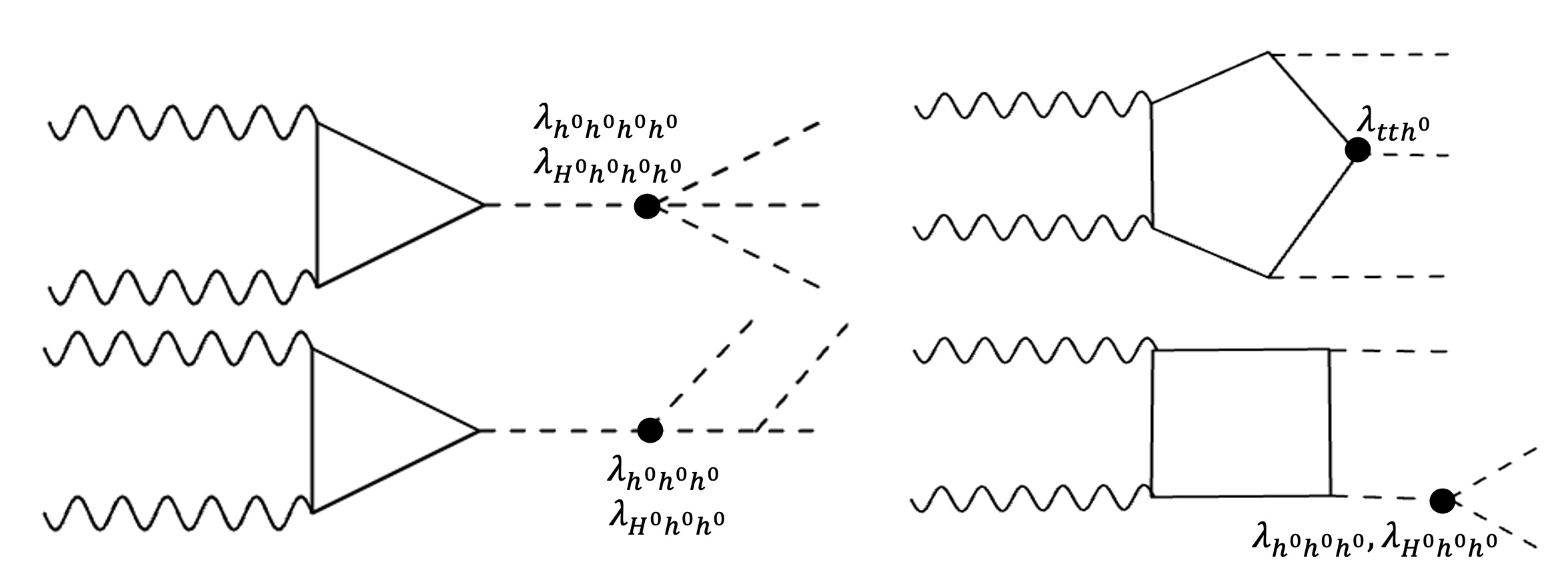
Figure 2: These Feynman diagrams illustrate the loop-induced production of three Higgs bosons in both the SM and the HTM. The wavy lines represent collinear photons, the dashed lines indicate scalar bosons, and the solid lines depict fermions and $W$-bosons. In the SM, these processes are facilitated by SM fermions and $W^{+}$-bosons. The HTM, in addition to the SM contributions, also includes contributions from charged Higgs bosons, as shown by the solid lines.

The UFO file generated from the FeynRules model is exported to GoSam-2.0, which automates the calculation of one-loop amplitudes for processes involving multiple particles. The analytic expression for the scattering amplitude of $\gamma\gamma\rightarrow h^{0}h^{0}h^{0}$ is computed using GoSam-2.0, which integrates tools such as QGRAF [89], FORM [90], spinney [91] and and haggies [92]. The amplitude involves loop integrals, which are reduced through the use of the Ninja [93], Golem95 [94, 95, 96], and Samurai [93], libraries. Ninja carried out the integral reduction through Laurent expansion, as detailed in Ref. [97, 98]. For further details, the author recommends consulting the Gosam-2.0 manual in Ref. [99]. After generating the large analytical expression, a numerical amplitude for this 2-to-3 process is produced using the provided inputs. To compute total cross-sections and kinematic distributions, we developed a Monte Carlo phase-space integration method based on the RAMBO algorithm [100], which utilizes isotropic phase-space sampling [101, 100, 102].

The production of triple Higgs via photon-photon collisions is a subprocess of $\mu^{+}\mu^{-}$ interactions at a muon collider. The total cross section for this process can therefore be determined from the following expression:

$$\sigma(s,h^{0}h^{0}h^{0})=\int d\tau\frac{d\mathcal{L}_{\gamma\gamma}}{d\tau}\hat{\sigma}\left(\hat{s}=\tau s,h^{0}h^{0}h^{0}\right),$$ (32)

along with the photon luminosity, which is expressed as

$$\tau\frac{d\mathcal{L}_{\gamma\gamma}}{d\tau}=\int_{0}^{1}dx_{1}x_{2}\Big{[}x_{1}f_{\gamma/\mu}(x_{1})x_{2}f_{\gamma/\mu}(x_{2})\Big{]}\delta(\tau-x_{1}x_{2}).$$ (33)

Where $\sqrt{\hat{s}}$ and $\sqrt{s}$ represent the center-of-mass energies of the $\gamma\gamma$ and $\mu^{+}\mu^{-}$ interactions, respectively. The distribution of photon energies emitted by a charged lepton, characterized by an energy fraction $x$ and an initial energy $\mathcal{E}$, adheres to the Weizsäcker-Williams spectrum [103, 104, 105], Eq. 34, also referred to as the Effective Photon Approximation (EPA) [106, 107, 108, 28, 109].

$$f_{\gamma/l}(x)\approx\frac{\alpha_{e}}{2\pi}P_{\gamma/l}(x)\ln{\frac{\mathcal{E}^{2}}{m_{l}^{2}}}\ .$$ (34)

The splitting functions are expressed as,

$$P_{\gamma/l}(x)=\frac{1+(1-x)^{2}}{x}:l\rightarrow\gamma,$$ (35)

and

$$P_{l/l}(x)=\frac{1+x^{2}}{1-x}:l\rightarrow l.$$ (36)

To validate our developed code, we computed the parton-level cross-section, $\hat{\sigma}(hhh)$, for the process $\gamma\gamma\rightarrow h^{0}h^{0}h^{0}$ within the SM and compared the results with those obtained using FormCalc. For the SM calculations, we used the smdiag model option available in GoSam-2.0. Both codes demonstrated excellent agreement.

V Results and Discussion

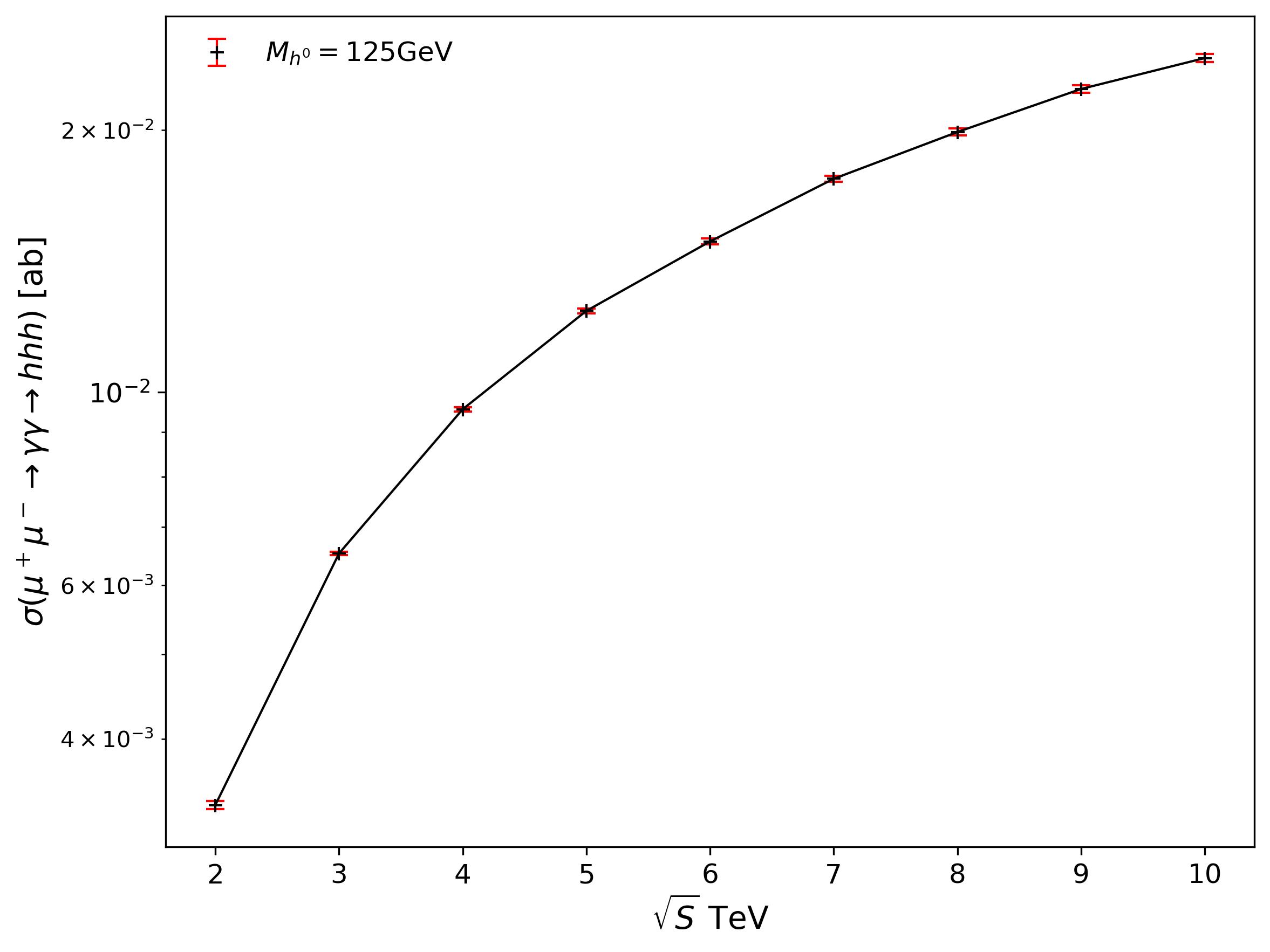
Figure 4: The cross-section for $h^{0}h^{0}h^{0}$ production in a muon collider for the SM via photon fusion as a function of the center-of-mass energy of the muon collider. The results are obtained using the leading-order EPA.

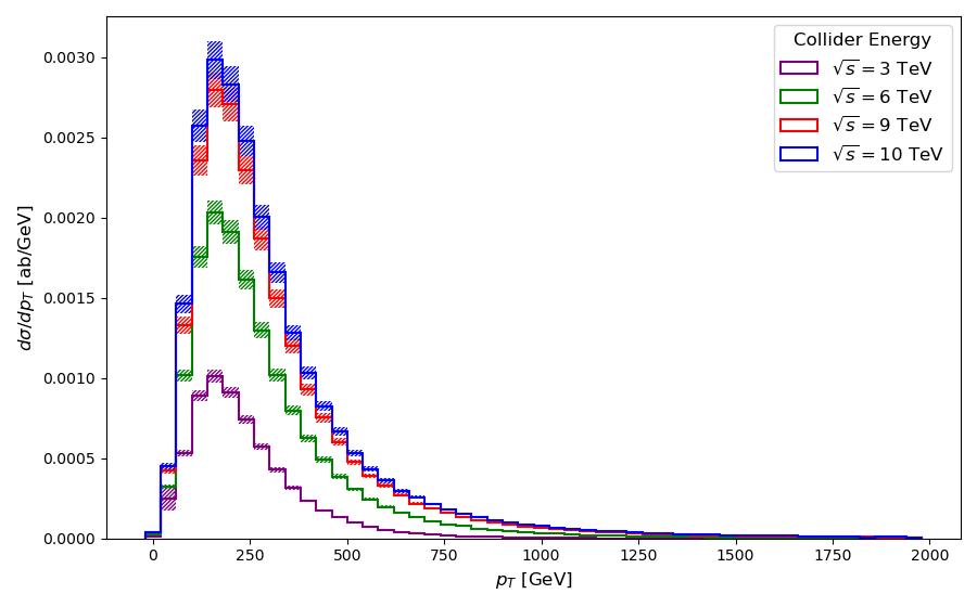
(a) Higgs transverse-momentum distribution.

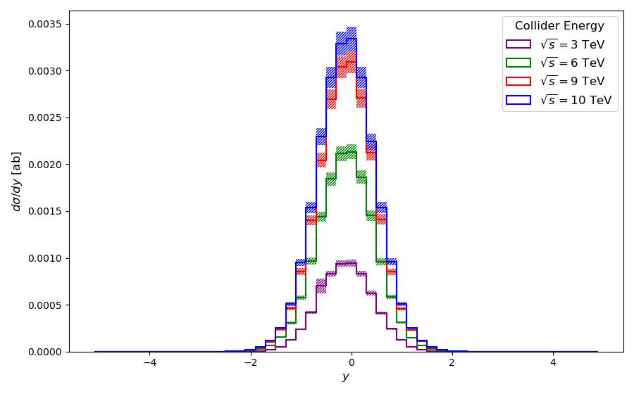
(b) Higgs rapidity distribution.

Figure 7: Higgs transverse-momentum (a) and rapidity (b) distributions for three-Higgs production via photon-induced processes in $\mu^{+}\mu^{-}$ collisions within the SM.

Our goal is to produce predictions for the production of three light Higgs bosons in $\mu^{+}\mu^{-}$ colliders via a $\gamma\gamma$ loop-induced process. In this section, we present the numerical results for triple Higgs production ($h^{0}h^{0}h^{0}$) via photon fusion in the HTM, focusing on cross-sections and kinematic distributions, and comparing them to SM predictions. In the previous section, we calculated the partonic cross-sections of $\gamma\gamma\rightarrow h^{0}h^{0}h^{0}$ within the range of $500\,\mathrm{GeV}\leq\sqrt{\hat{s}_{\gamma\gamma}}\leq 1.5\,\mathrm{TeV}$ in the SM as part of the code validation process. The partonic cross-section $\hat{\sigma}(\gamma\gamma\rightarrow h^{0}h^{0}h^{0})$ reaches its maximum value at approximately $750\,\mathrm{GeV}$. The results obtained, as shown in Fig. 3, from FormCalc and GoSam-2.0 are in agreement with each other and also align with the calculations in Ref. [32]. In the second step, We calculated the total cross-section for $\mu^{+}\mu^{-}\rightarrow\gamma\gamma\rightarrow h^{0}h^{0}h^{0}$ and found that the results generated by Gosam-2.0 do not agree with Ref. [32]. In Fig. 4, the full cross sections for SM predictions are shown as a function of center of mass energy of the muon collider with the Monte Carlo errors. The cross-section in the SM ranges from $3.35\times 10^{-3}$ to $2.42\times 10^{-2}$ ab, as shown in Fig. 4. With integrated luminosities between $0.4$ and $10$ ab^-1, the expected number of events is less than one. This implies that SM three-Higgs production via photon fusion is not observable at the center-of-mass energies considered here. In Fig. 7, we present the transverse momentum distribution with rapidity, selecting events with transverse momentum $P_{T}>0$ and rapidity $|y|<5$. The distribution shows peaks at different collider energies, around 130 GeV.

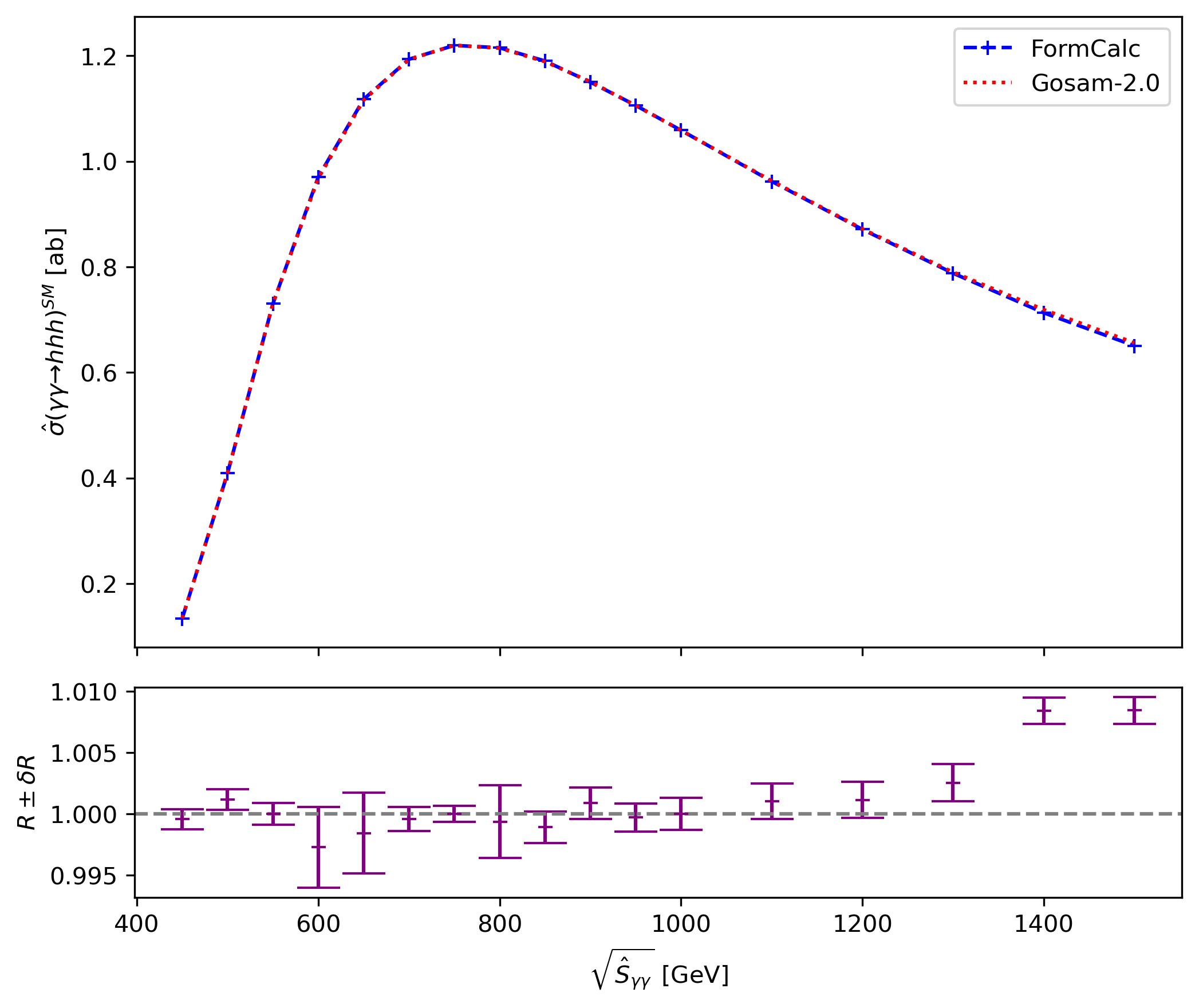
Figure 3: Partonic cross-sections as a function of the center-of-energy of $\gamma\gamma$, $\sqrt{\hat{s}_{\gamma\gamma}}$. This shows the results obtained from FormCalc and Gosam-2.0. The lower panel presents $R=\hat{\sigma}_{\texttt{FormCalc}}/\hat{\sigma}_{\texttt{Gosam-2.0}}$ with errors.

Table 1: The singly charged Higgs and pseudoscalar masses were obtained using Eq. 24 and Eq. 22, respectively, for both Scenario I and Scenario II. For the second scenario, the mass of the heavy Higgs was obtained from Eq. 31. Here, we have dropped the max and min labels for simplicity. For Scenario I, we have chosen $\epsilon_{P}=4.248\times 10^{-3}$, whereas for Scenario II, it is $3.2822\times 10^{-3}$ when evaluating the singly charged Higgs mass using Eq. 23 and Eq. 24.

. Scenario $\alpha$ $M_{h^{0}}$ $M_{H^{0}}$ $M_{A^{0}}$ $M_{H^{\pm\pm}}$ $M_{H^{\pm}}$ I 0 $125$ 376.5000 376.5124431 290.5 336.26207047 II $\pi/4$ 125 126.0204 125.5153850 240.0 191.51107095

Table 2: The calculated Lagrangian parameters are based on the inputs from Table 1. The sign of the $\lambda_{4}$ parameter is a discriminator for the hierarchy between doubly and singly charged Higgs bosons.

Scenario	$\lambda$	$\lambda_{1}$	$\lambda_{2}$	$\lambda_{3}$	$\lambda_{4}$	$\mu$
I	0.51	2.7	5.61	-5.61	1.89	3.31
II	0.52	1.382	2.514	-2.514	-1.382	0.368

In the HTM, at the one-loop level, the process $\gamma\gamma\rightarrow h^{0}h^{0}h^{0}$ is mediated by $H^{\pm}$ and $H^{\pm\pm}$, unlike in the SM. This process relies on the couplings $H^{0}h^{0}h^{0}$ and $H^{0}h^{0}h^{0}h^{0}$. The Feynman diagrams in Fig. 2 show that the triangle diagrams are particularly sensitive to these couplings. Based on the two scenarios described in Sec. III, we have established the input sets shown in Table 1. In Scenario I, when the mixing angle between $h^{0}$ and $H^{0}$ is minimized, the amplitude is consequently reduced. The final states of the process will be SM-like Higgs bosons as $\alpha\rightarrow 0$, which is characteristic of the HTM. One main reason for the suppression of the amplitude is that the $H^{0}h^{0}h^{0}$ and $H^{0}h^{0}h^{0}h^{0}$ couplings are approaching their weak-coupling decoupling limits [110]. This scenario is not favorable for detecting the heavy Higgs boson and examining its contributions. This issue can be addressed in Scenario I by setting the intermediate state on-shell and ensuring that the threshold $M_{H^{0}}\geq 3M_{h^{0}}$ is met. Unfortunately, these contributions are not maximally enhanced, resulting in a moderate increase in the cross sections due to the relatively weak couplings mentioned earlier. Nevertheless, this enhancement improves the likelihood of observing the heavy Higgs boson and examining its contributions, which is essential for gaining a more comprehensive understanding of the HTM.

However, we cannot overlook the contributions of $H^{0}$ and its couplings to neutral scalars. Therefore, we have established a second scenario (Scenario II) where $\alpha=\pi/4$. This scenario has some limitations, as it cannot reach large mass scales for the heavy Higgs. Our parameter scanning method shows that $M_{H^{0}}$ can reach up to approximately 150 GeV for $\cos{\alpha}\in[0,0.9)$ at $v_{\Delta}=8~\mathrm{GeV}$, as shown in panel (b) of Fig. 12. In the second scenario, we keep $v_{\Delta}=1,\mathrm{GeV}$ and allow the heavy Higgs to be slightly heavier than the SM-like Higgs, as discussed in Ref. [73]. Although the decay $H^{0}\rightarrow h^{0}h^{0}$ is kinematically forbidden, the $H^{0}h^{0}h^{0}$ and $H^{0}h^{0}h^{0}h^{0}$ couplings are significantly larger than those in Scenario I. The significant increase in the $H^{0}h^{0}h^{0}$ coupling in Scenario II compared to Scenario I, by a factor of $\sim 743$ (Table 3), allows $H^{0}$ to still appear as a virtual (off-shell [7]) propagator in loop diagrams contributing to $\gamma\gamma\to h^{0}h^{0}h^{0}$. These couplings are much stronger due to the specific parameter settings, which enhance the interactions involving the heavy Higgs. This dramatic increase suggests that Scenario II could provide a more favorable environment for studying the effects and contributions of the heavy Higgs boson, despite its limitations in reaching larger mass scales. To analyze the scalar couplings in these calculations, we used the expressions presented in Sec. A, which were evaluated in the cross-section calculations for each scenario.

Table 3 provides a comprehensive comparison of the trilinear and quartic neutral scalar couplings between the SM and the two scenarios in the HTM with $\alpha=0$ and $\alpha=\pi/4$. This comparison is crucial for understanding the variations in coupling strengths under different parameter settings. The table highlights how the $h^{0}h^{0}h^{0}$ and $h^{0}h^{0}h^{0}h^{0}$ couplings in Scenario I are closer to the SM values, while those in Scenario II show more substantial deviations.

In Scenario I, the couplings $\lambda^{HTM}_{h^{0}h^{0}h^{0}h^{0}}$ and $\lambda^{HTM}_{h^{0}h^{0}h^{0}}$ are very close to the SM values ($0.98\times\lambda_{h^{0}h^{0}h^{0}h^{0}}^{SM}$ and $0.98\times\lambda_{h^{0}h^{0}h^{0}}^{SM}$, respectively), indicating minimal mixing between the doublet and triplet Higgs fields. In contrast, Scenario II shows significant deviations from the SM, with $\lambda^{HTM}_{h^{0}h^{0}h^{0}h^{0}}$ reduced to $\frac{1}{4}\times\lambda_{h^{0}h^{0}h^{0}h^{0}}^{SM}$ and $\lambda^{HTM}_{h^{0}h^{0}h^{0}}$ reduced to $0.353\times\lambda_{h^{0}h^{0}h^{0}}^{SM}$.

Table 3: Comparison of trilinear and quartic neutral scalar couplings between the SM and the two scenarios in the HTM. The first three rows compare the scalar couplings between Scenarios I and II, while the last two rows show the comparison of these couplings in the scenarios with the SM couplings separately.

Coupling Expression	Scenario I ($\alpha=0$)	Scenario II ($\alpha=\pi/4$)
$\lambda_{hhhh}^{HTM}(\alpha)$	$\approx 4\times\lambda_{hhhh}^{HTM}(\alpha=\pi/4)$	$\approx 0$
$\lambda_{hhhH}^{HTM}(\alpha)$	$\approx 0$	$\gg\lambda_{hhhH}^{HTM}(\alpha=0)$
$\lambda_{hhH}^{HTM}(\alpha)$	$\approx 0$	$743\times\lambda_{hhH}^{HTM}(\alpha=0)$
$\lambda_{hhhh}^{HTM}(\alpha)$	$0.98\times\lambda_{hhhh}^{SM}$	$\frac{1}{4}\times\lambda_{hhhh}^{SM}$
$\lambda_{hhh}^{HTM}(\alpha)$	$0.98\times\lambda_{hhh}^{SM}$	$0.353\times\lambda_{hhh}^{SM}$

In addition to trilinear and quartic scalar couplings, Feynman diagrams with box, triangle, and pentagon topologies are particularly sensitive to the Higgs couplings with fermions and $W^{\pm}$ bosons. Evaluating their contributions to the cross section is straightforward, as the coupling between the neutral Higgs boson and fermions, $h^{0}f\bar{f}$, in the HTM is modified relative to the SM and is given by:

$$\cos{\alpha}\left(1+\frac{2v_{\Delta}^{2}}{v_{\Phi}^{2}}\right)^{1/2}.$$ (37)

Notably, in two scenarios, the coupling strength follows the relation:

$$\lambda^{HTM}_{h^{0}f\bar{f}}(\alpha=0)\approx\sqrt{2}\times\lambda^{HTM}_{h^{0}f\bar{f}}(\alpha=\pi/4).$$ (38)

Similarly, the Higgs coupling to $W^{+}W^{-}$ bosons in the HTM is given by:

$$\lambda_{h^{0}W^{+}W^{-}}^{HTM}=\frac{2M_{W}^{2}}{v^{2}}(\cos{\alpha}\,v_{\Phi}+2\sin{\alpha}\,v_{\Delta}).$$ (39)

which shows that:

$$\lambda^{HTM}_{h^{0}W^{+}W^{-}}(\alpha=0)=\sqrt{2}\times\lambda^{HTM}_{h^{0}W^{+}W^{-}}(\alpha=\pi/4).$$ (40)

From these expressions, it is evident that in the first scenario ($\alpha=0$), both the Higgs-fermion and Higgs-gauge boson couplings are stronger compared to the second scenario ($\alpha=\pi/4$) and the SM.

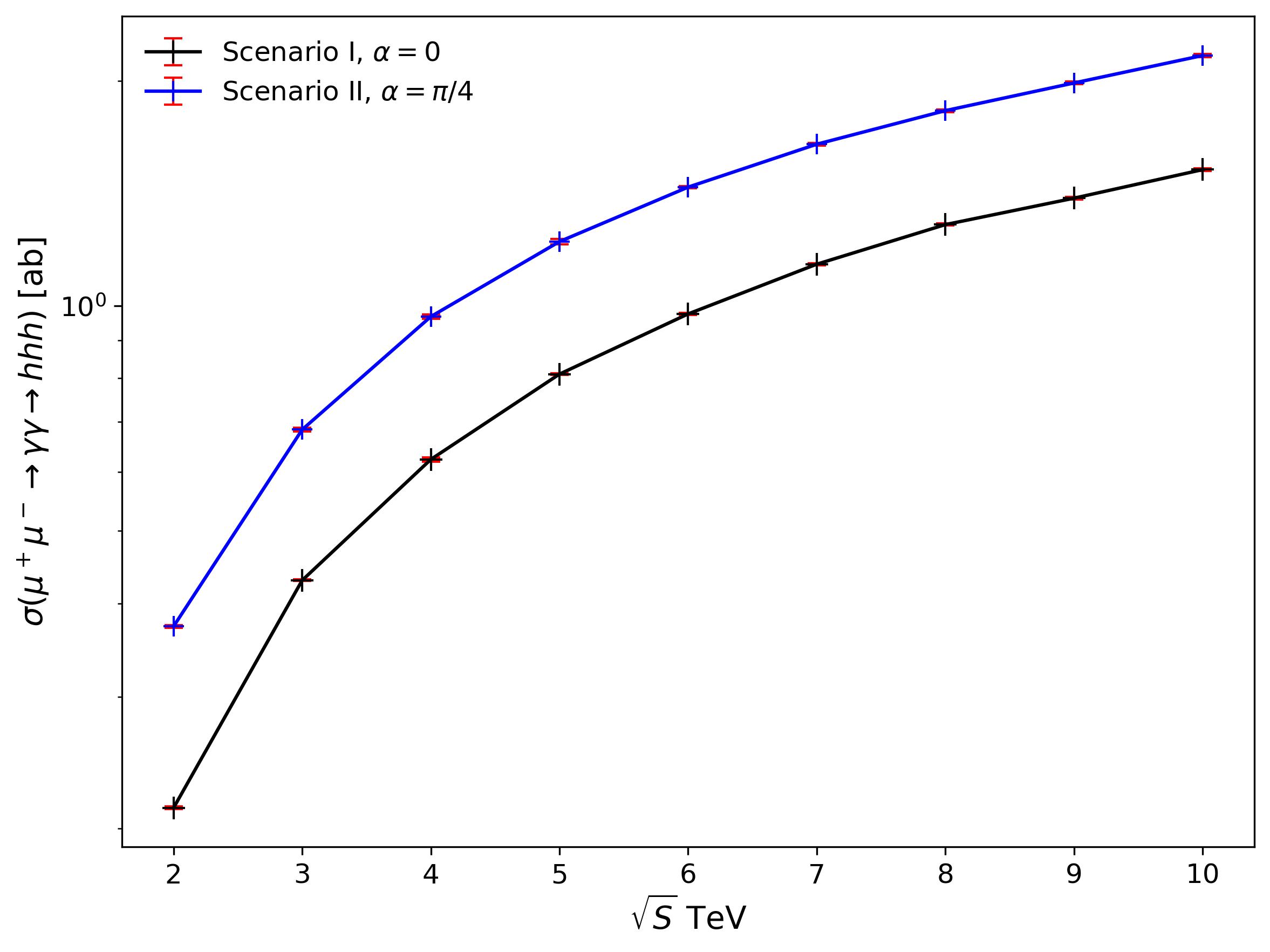
Figure 5: The cross-section for $h^{0}h^{0}h^{0}$ production in a muon collider for the HTM via photon fusion as a function of the center-of-mass energy of the muon collider. The results are obtained using the leading-order EPA.

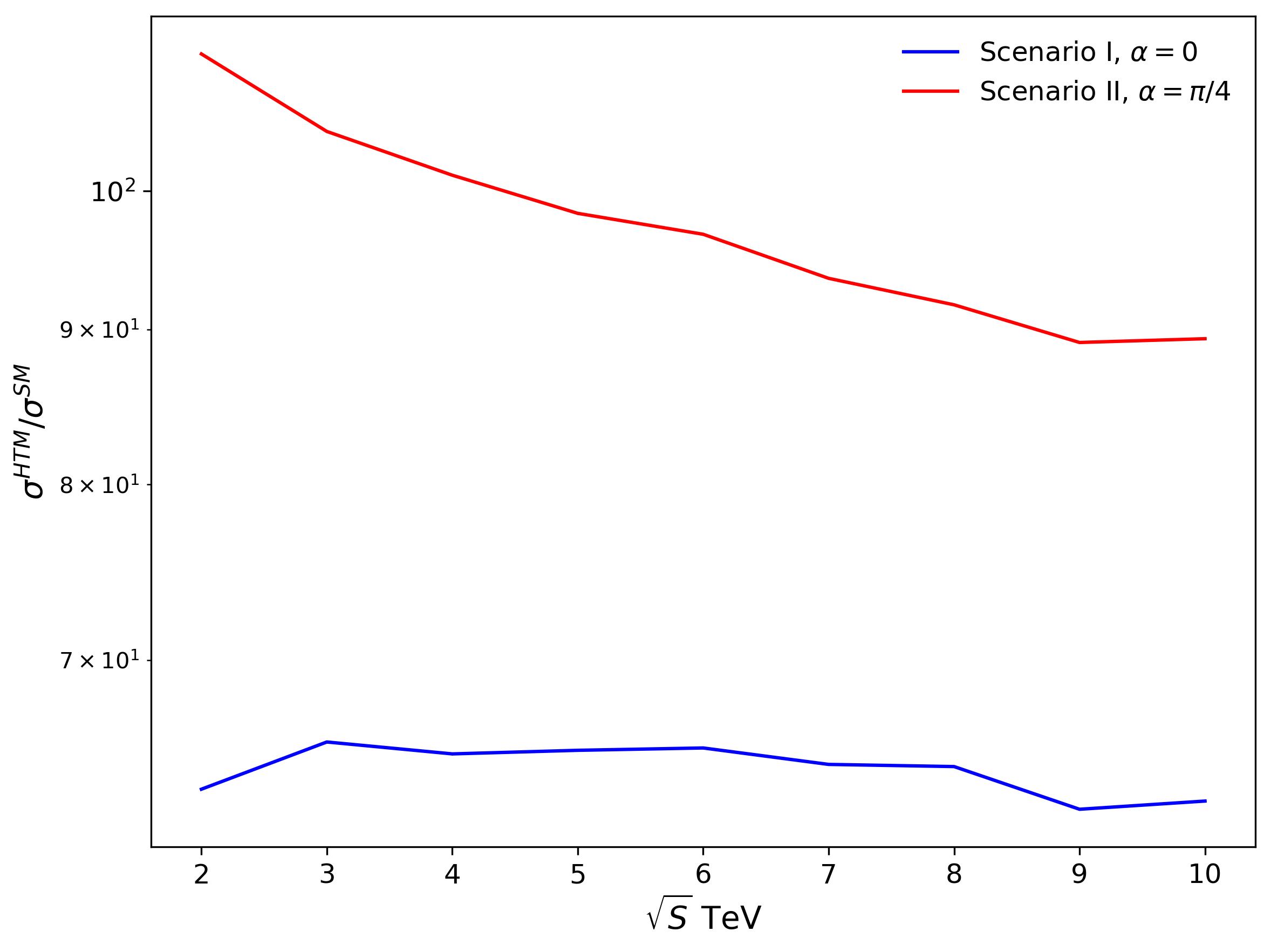
Figure 6: The ratio of $\sigma^{HTM}/\sigma^{SM}$ as a function of center-of-mass energy shows a significant enhancement in the cross sections for both scenarios compared to the SM.

The cross sections for the process $\mu^{+}\mu^{-}\rightarrow\gamma\gamma\rightarrow h^{0}h^{0}h^{0}$ at a muon collider with $\sqrt{s}=2-10$ TeV are shown in Fig. 5 for each scenario. Notably, the cross sections in Scenario II exhibit a significant enhancement compared to Scenario I.

In Fig. 6, the cross sections for both scenarios are compared to the SM predictions. For Scenario I, the ratio of the HTM cross section to the SM cross section is in the range $50<\sigma^{HTM}/\sigma^{SM}<60$, whereas for Scenario II, this ratio increases to $90<\sigma^{HTM}/\sigma^{SM}<110$. This suggests that the coupling $\lambda_{H^{0}h^{0}h^{0}}$ plays a crucial role in enhancing the production cross section.

Figs. 8 and 9 present the transverse momentum $P_{T}$ distributions of the Higgs boson carrying the highest $P_{T}$, ($P_{T}>0$ and $|y|<5$), at center-of-mass energies of $\sqrt{s}=3,6,9,$ and $10$ TeV. In Scenario II, the peak of the transverse momentum distribution is higher compared to both Scenario I and the SM. Meanwhile, the rapidity distributions exhibit a similar shape across different center-of-mass energies.

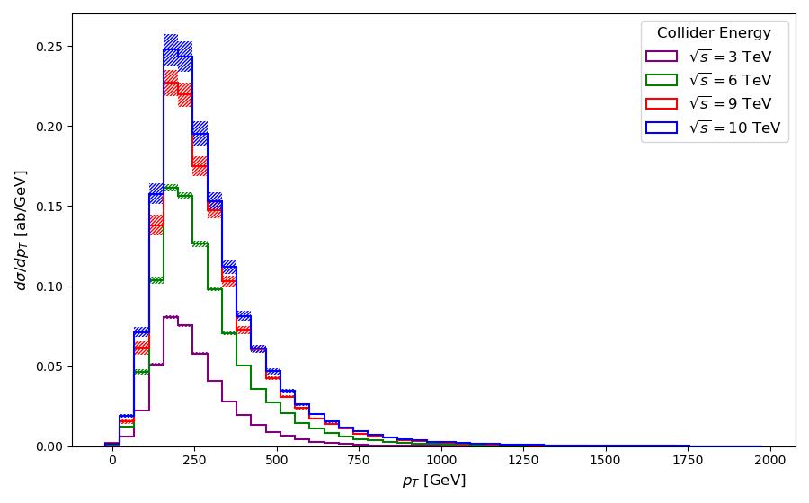
(a) Higgs transverse-momentum distribution.

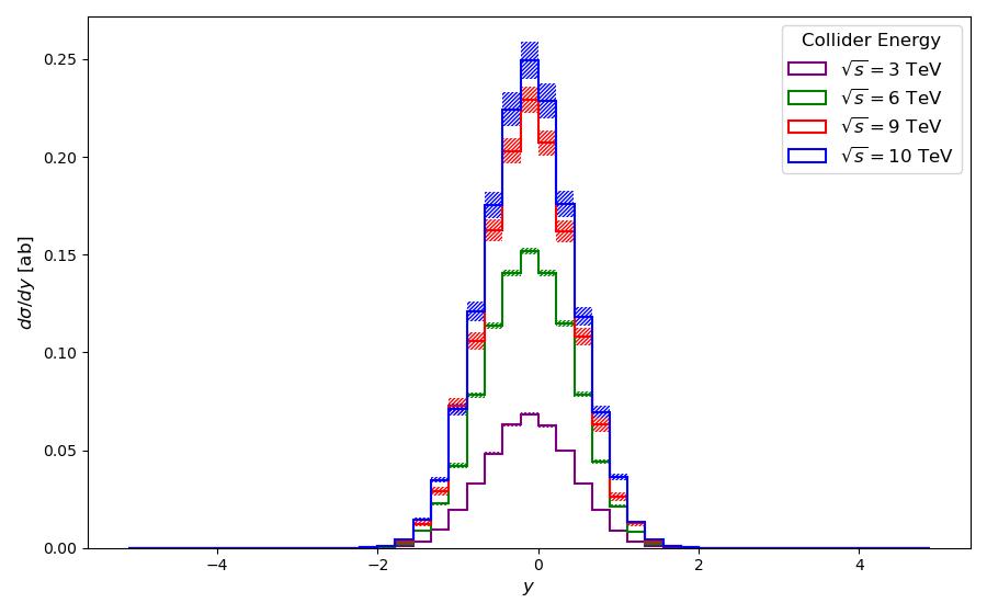
(b) Higgs rapidity distribution.

Figure 8: Higgs transverse-momentum (a) and rapidity (b) distributions for three-Higgs production via photon-induced processes in $\mu^{+}\mu^{-}$ collisions within the HTM under scenario I.

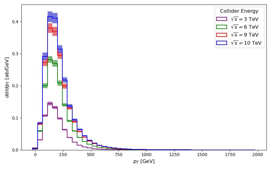
(a) Higgs transverse-momentum distribution.

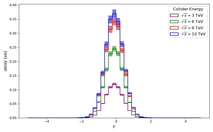
(b) Higgs rapidity distribution.

Figure 9: Higgs transverse-momentum (a) and rapidity (b) distributions for three-Higgs production via photon-induced processes in $\mu^{+}\mu^{-}$ collisions within the HTM under scenario II

Additionally, the charged Higgs mass hierarchies differ between the two scenarios. In Scenario I, the hierarchy is $M_{H^{\pm}}>M_{H^{\pm\pm}}$, with the neutral Higgs masses approximately satisfying $M_{H^{0}}\approx M_{A^{0}}$. In contrast, Scenario II exhibits a reversed hierarchy, where $M_{H^{\pm}}<M_{H^{\pm\pm}}$ and $M_{H^{0}}>M_{A^{0}}$.

Table 4: Event counts ($N$) for three Higgs production in $\mu^{+}\mu^{-}$ colliders. The event count obtained by $N=\sigma\mathcal{L}$ [111].

$\sqrt{s}~(\mathrm{TeV})$	Luminosity $[\text{ab}^{-1}$]	$N_{\text{Scenario I}}$	$N_{\text{Scenario II}}$
2	0.4	0	0
3	1	0	1
4	2	2	2
5	3	3	4
6	4	4	6
7	5	6	9
8	7	9	13
9	9	13	18
10	10	16	22

The observability of these scenarios at different muon collider energies is summarized in Table 4. In Scenario I, the event rate is too low for detection at $\sqrt{s}=2$ TeV and $\sqrt{s}=3$ TeV, making it unobservable at these energies. However, in Scenario II, the process remains unobservable only at $\sqrt{s}=2$ TeV, while higher energies yield a sufficient number of events for detection.

VI Conclusions

The study of multi-Higgs final states, such as $h^{0}h^{0}h^{0}$ production at $\mu^{+}\mu^{-}$ colliders, provides a means to probe the Higgs potential within the HTM and extract information about its underlying parameters and interactions, offering insights into physics beyond the SM. In the HTM, double and triple Higgs production involves trilinear and quartic charged Higgs couplings, which are absent in the SM and many BSM scenarios. Their contributions can be explored through the process $\gamma\gamma\rightarrow h^{0}h^{0}h^{0}$, and to investigate this, we have calculated the total cross sections and kinematic distributions for $\mu^{-}\mu^{-}\rightarrow\mu^{+}\mu^{-}h^{0}h^{0}h^{0}$, mediated by the one-loop-induced $\gamma\gamma\rightarrow h^{0}h^{0}h^{0}$ process using the EPA.

Prior to performing calculations, we established our own parameter scanning process and Monte Carlo code using Fortran and Gosam-2.0 for $\alpha\in[-\pi/2,\pi/2]$, where the input parameters for the Monte Carlo simulation are the masses of the scalar Higgs bosons. Our parameter scanning method determines the upper and lower bounds of $M_{H^{\pm}}$, $M_{A^{0}}$, and $M_{H^{0}}$ based on $M_{H^{\pm\pm}}$, $v_{\Delta}$ and $\alpha$.

To modify Gosam-2.0 for Monte Carlo simulations, we utilized the RAMBO algorithm and incorporated the EPA as a Fortran subroutine. Our calculations were performed by establishing two benchmark parameter sets (Scenario I and Scenario II), with a particular focus on the mixing angle $\alpha$ between the heavy Higgs and the SM-like Higgs. In Scenario I, we obtained cross sections and transverse momentum distributions, including rapidity dependence, for small values of $\alpha$, corresponding to the decoupling limit of $H^{0}h^{0}h^{0}$ and $H^{0}h^{0}h^{0}h^{0}$ interactions.

In Scenario II, we set $\alpha=\pi/4$ and assumed $M_{H^{0}}\sim M_{h^{0}}$. Compared to Scenario I, all trilinear scalar couplings in Scenario II are generally smaller, except for the $h^{0}h^{0}h^{0}H^{0}$ and $h^{0}h^{0}H^{0}$ couplings, which remain sizable. Moreover, in this scenario, the Higgs boson exhibits somewhat fermiophobic behavior, as it has reduced couplings to electroweak gauge bosons and fermions compared to both Scenario I and the SM.

Despite this behavior, the dominance of heavy Higgs couplings to the SM-like Higgs in Scenario II leads to a significant enhancement in the production cross section, yielding $\sigma^{HTM}/\sigma^{SM}>90$, whereas in Scenario I, we find $\sigma^{HTM}/\sigma^{SM}>48$. For an integrated luminosity given by $\mathcal{L}\sim(\sqrt{s}/10~\mathrm{TeV})^{2}\times 10~\mathrm{ab}^{-1}$, ranging from $2$ to $10~\mathrm{ab}^{-1}$, all scenarios in the HTM predict more than one observable event in muon collider experiments, whereas the SM prediction remains undetectable within this center-of-mass energy range.

VII DISCLAIMER

The authors acknowledge the assistance of generative AI, specifically Microsoft Copilot, which Wichita State University has provided access to for researchers. The improvement of the manuscript’s readability, correction of flaws, and fixing of LaTeX  code bugs were facilitated by the use of this generative AI tool.

Appendix A SCALAR HIGGS COUPLINGS IN TERMS OF $\lambda$, $\lambda_{i}$s and VEVs

The following expressions represent the scalar couplings evaluated in the cross-section calculations for Scenario I.

$$\lambda_{h^{0}h^{0}h^{0}h^{0}}^{HTM}=3\frac{\lambda}{2}$$ (41)

$$\lambda_{h^{0}h^{0}h^{0}H^{0}}^{HTM}\approx 0$$ (42)

$$\lambda_{h^{0}h^{0}h^{0}}^{HTM}=3\frac{\lambda v_{\Phi}}{2}$$ (43)

$$\lambda_{h^{0}h^{0}H^{0}}^{HTM}\approx\sqrt{2}\mu-(\lambda_{1}+\lambda_{4})v_{\Delta}$$ (44)

$$\lambda_{h^{0}H^{\pm}H^{\pm}}^{HTM}\approx-(\lambda_{1}+\lambda_{4}/2)v_{\Phi}-2\sqrt{2}\mu\frac{v_{\Delta}}{v_{\Phi}}$$ (45)

$$\lambda_{h^{0}H^{\pm\pm}H^{\pm\pm}}^{HTM}\approx\lambda_{1}v_{\Phi}$$ (46)

$$\lambda_{h^{0}h^{0}H^{\pm}H^{\pm}}^{HTM}\approx-\left(\lambda_{1}+\frac{\lambda_{4}}{2}\right)$$ (47)

$$\lambda_{h^{0}h^{0}H^{\pm\pm}H^{\pm\pm}}^{HTM}\approx\lambda_{1}$$ (48)

The following expressions represent the scalar couplings evaluated in the cross-section calculations for Scenario II.

$$\lambda_{h^{0}h^{0}h^{0}h^{0}}^{HTM}=3\frac{\lambda}{8}+\frac{3}{2}(\lambda_{1}+\lambda_{2}+\lambda_{3}+\lambda_{4})$$ (49)

$$\lambda_{h^{0}h^{0}h^{0}H^{0}}^{HTM}\approx\frac{3}{8}\lambda-\frac{3}{2}(\lambda_{2}+\lambda_{3})$$ (50)

$$\lambda_{h^{0}h^{0}h^{0}}^{HTM}=-\frac{1}{8}\Big{\{}12\mu-3\sqrt{2}(\lambda+2\lambda_{1}+2\lambda_{4})\Big{\}}v_{\Phi}$$

$$+\frac{3}{2\sqrt{2}}\Big{\{}\lambda_{1}+\lambda_{4}+2(\lambda_{2}+\lambda_{3})\Big{\}}v_{\Delta}$$ (51)

$$\lambda_{h^{0}h^{0}H^{0}}^{HTM}=\frac{1}{8}\Big{\{}-4\mu+\sqrt{2}(3\lambda-2\lambda_{1}-2\lambda_{4})\Big{\}}v_{\Phi}$$

$$+\frac{1}{2\sqrt{2}}\Big{\{}\lambda_{1}+\lambda_{4}-6(\lambda_{2}+\lambda_{3})\Big{\}}v_{\Delta}$$ (52)

$$\lambda_{h^{0}H^{\pm}H^{\pm}}^{HTM}=-\frac{1}{\sqrt{2}}\left(\lambda_{1}+\frac{\lambda_{4}}{2}\right)v_{\Phi}$$

$$+\Big{\{}\frac{-2(\lambda_{2}+\lambda_{3})+\lambda_{4}}{\sqrt{2}}-\frac{\mu}{v_{\Phi}}\Big{\}}v_{\Delta}$$ (53)

$$\lambda_{h^{0}H^{\pm\pm}H^{\pm\pm}}^{HTM}=-\frac{\lambda_{1}}{\sqrt{2}}v_{\Phi}-2\sqrt{2}\lambda_{2}v_{\Delta}$$ (54)

$$\lambda_{h^{0}h^{0}H^{\pm}H^{\pm}}^{HTM}=-\frac{1}{4}\left(2\lambda_{1}+4(\lambda_{2}+\lambda_{3})-\lambda_{4}\right)+\frac{\lambda_{4}v_{\Delta}}{v_{\Phi}}$$ (55)

$$\lambda_{h^{0}h^{0}H^{\pm\pm}H^{\pm\pm}}^{HTM}\approx\lambda_{2}+\frac{\lambda_{1}}{2}$$ (56)

Appendix B Parameter Scanning and Model Variables: Plots and Analysis

The following plots show the values of $\lambda$, $M_{H^{\pm}}^{\text{max}}$, $M_{A^{0}}^{\text{max}}$ in Fig. 10 and Fig. 11, and $M_{H^{0}}^{\text{max}}$ in Fig. 12, depending on the parameter scanning method discussed in Sec. III. The corresponding $\cos{\alpha}$ ranges are $(0.9,1]$, $[-1,0)$, and $[0,0.9]$, respectively.

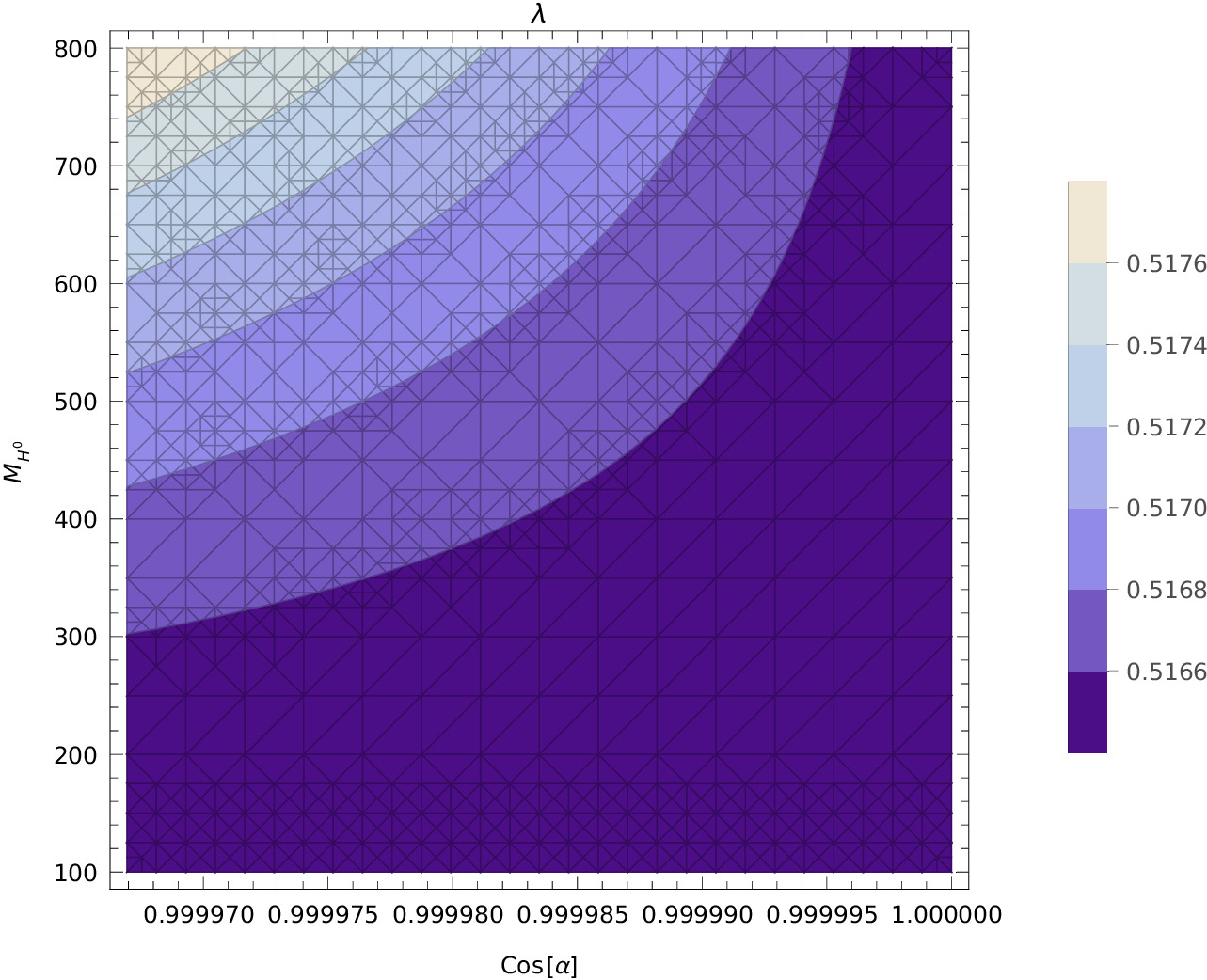
(a)

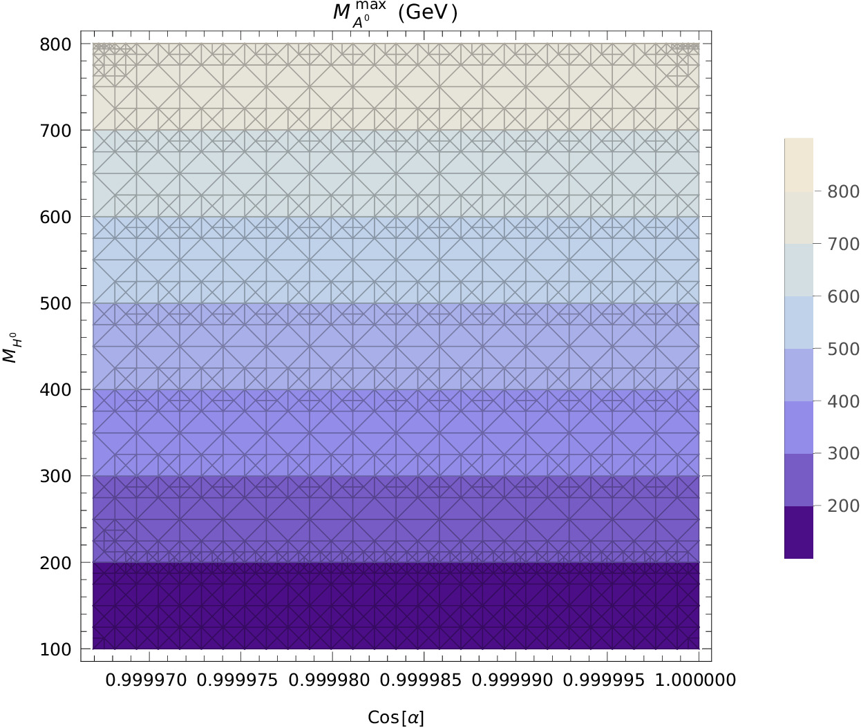
(b)

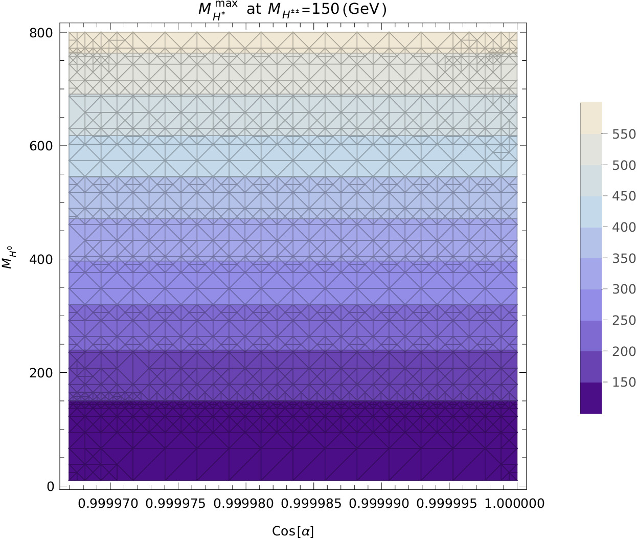
(c)

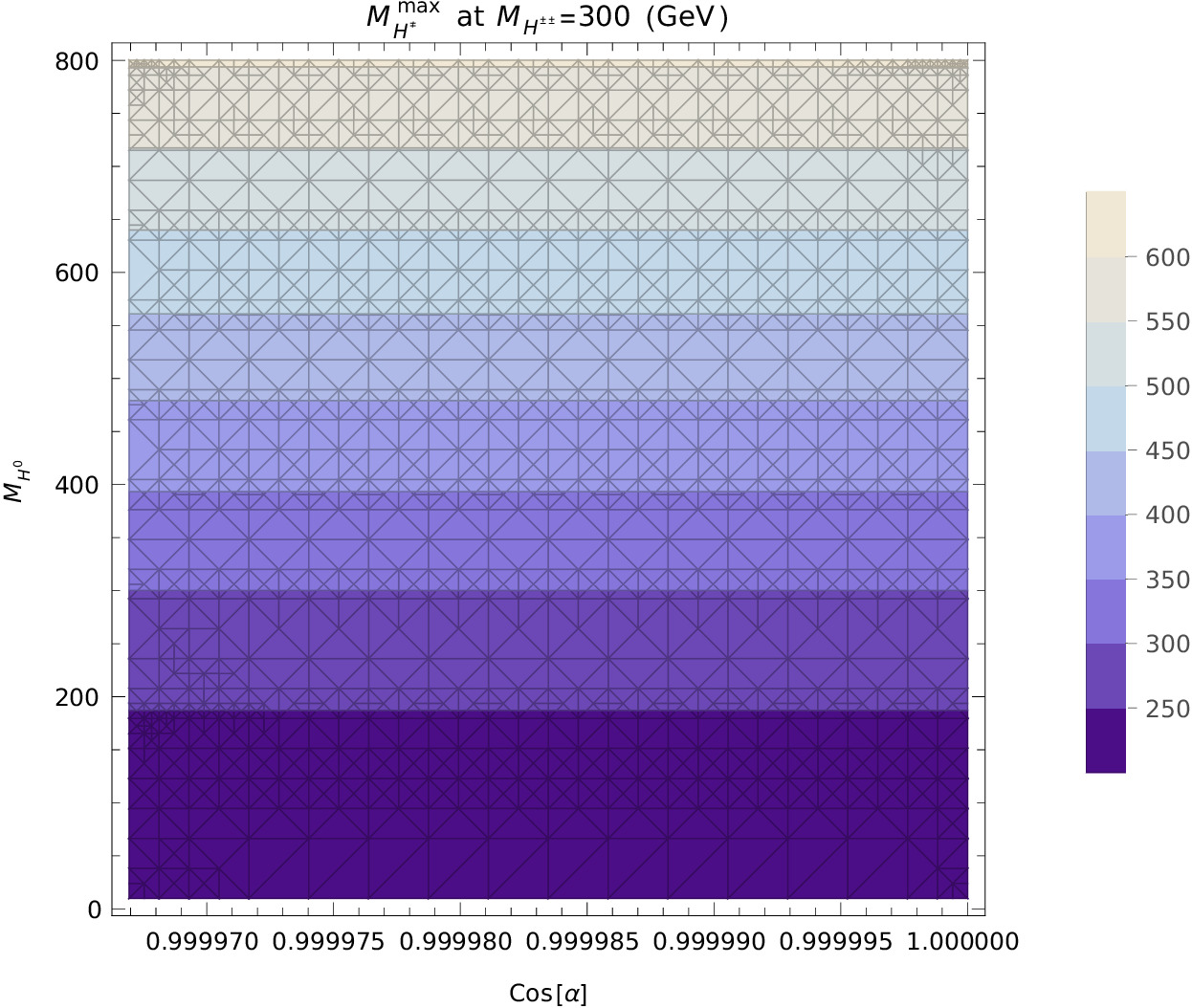
(d)

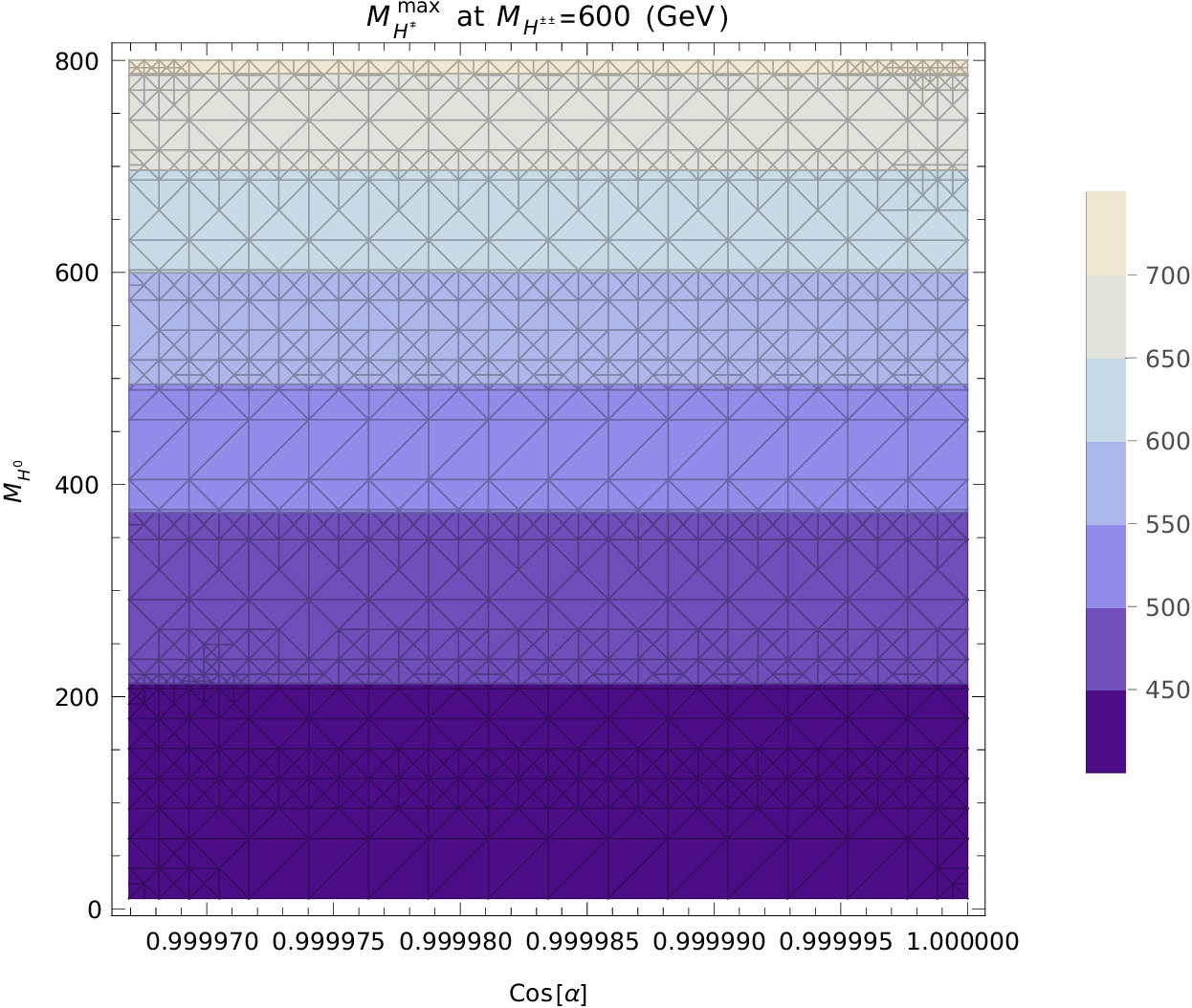
(e)

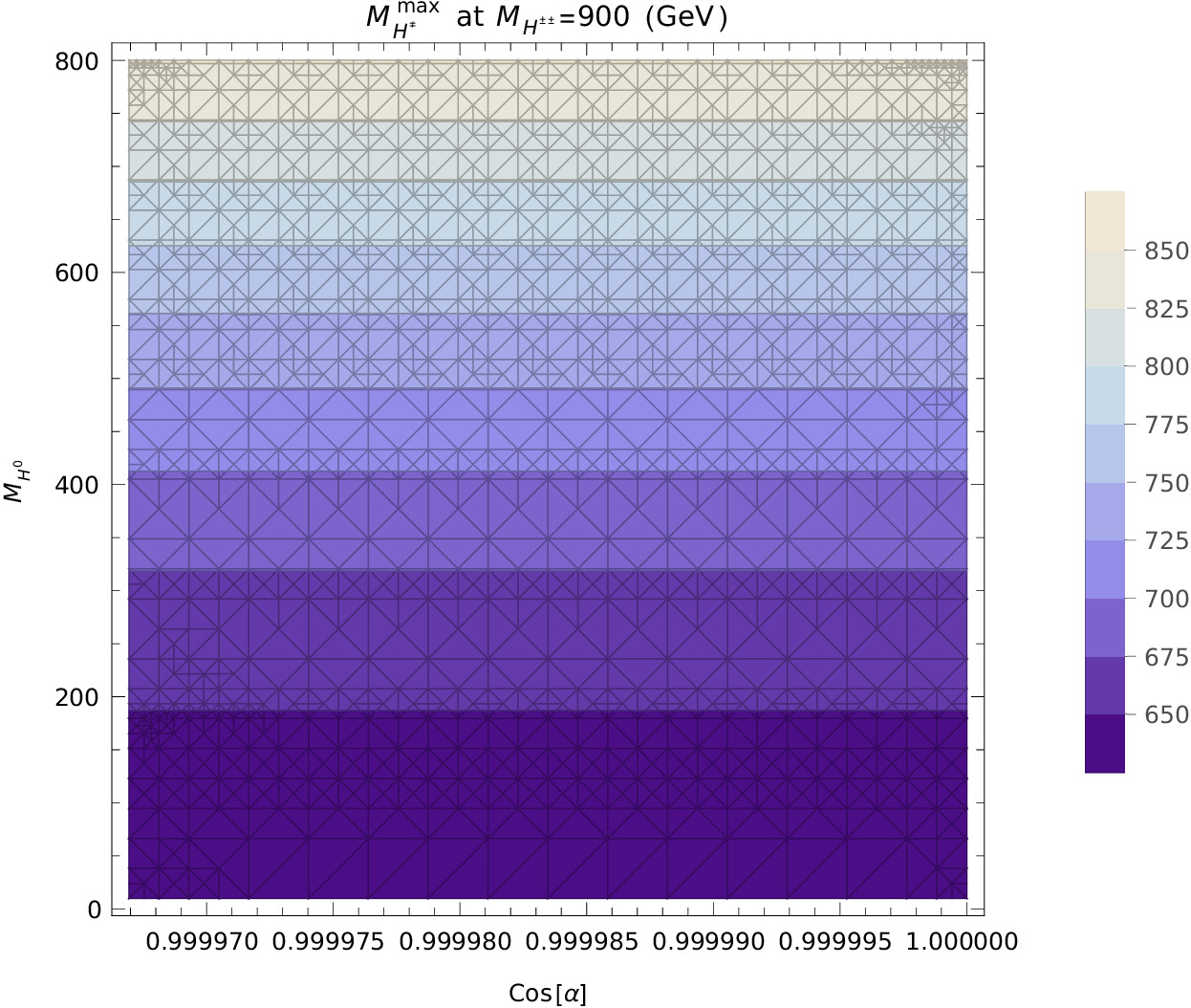
(f)

Figure 10: This figure presents the parameter $\lambda$ (panel (a)), $\mathrm{max}(M_{A^{0}})$ (panel (b)), and $M_{H^{\pm}}$ (panels (c), (d), (e), and (f)) as functions of $M_{h^{0}}$ and $\cos{\alpha}\rightarrow 1$, with $M_{h^{0}}=125\,\mathrm{GeV}$.

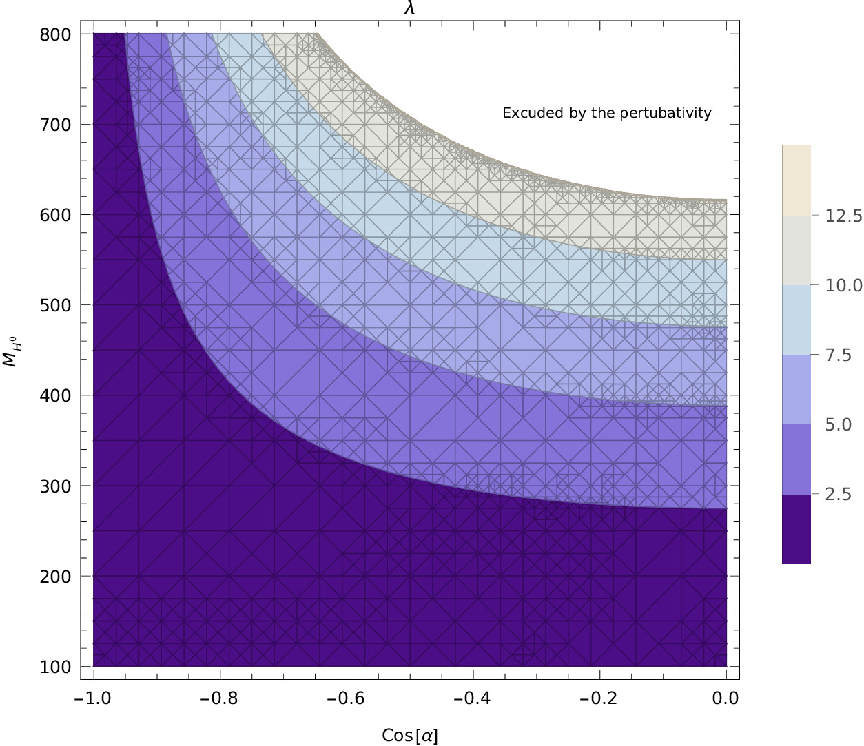
(a)

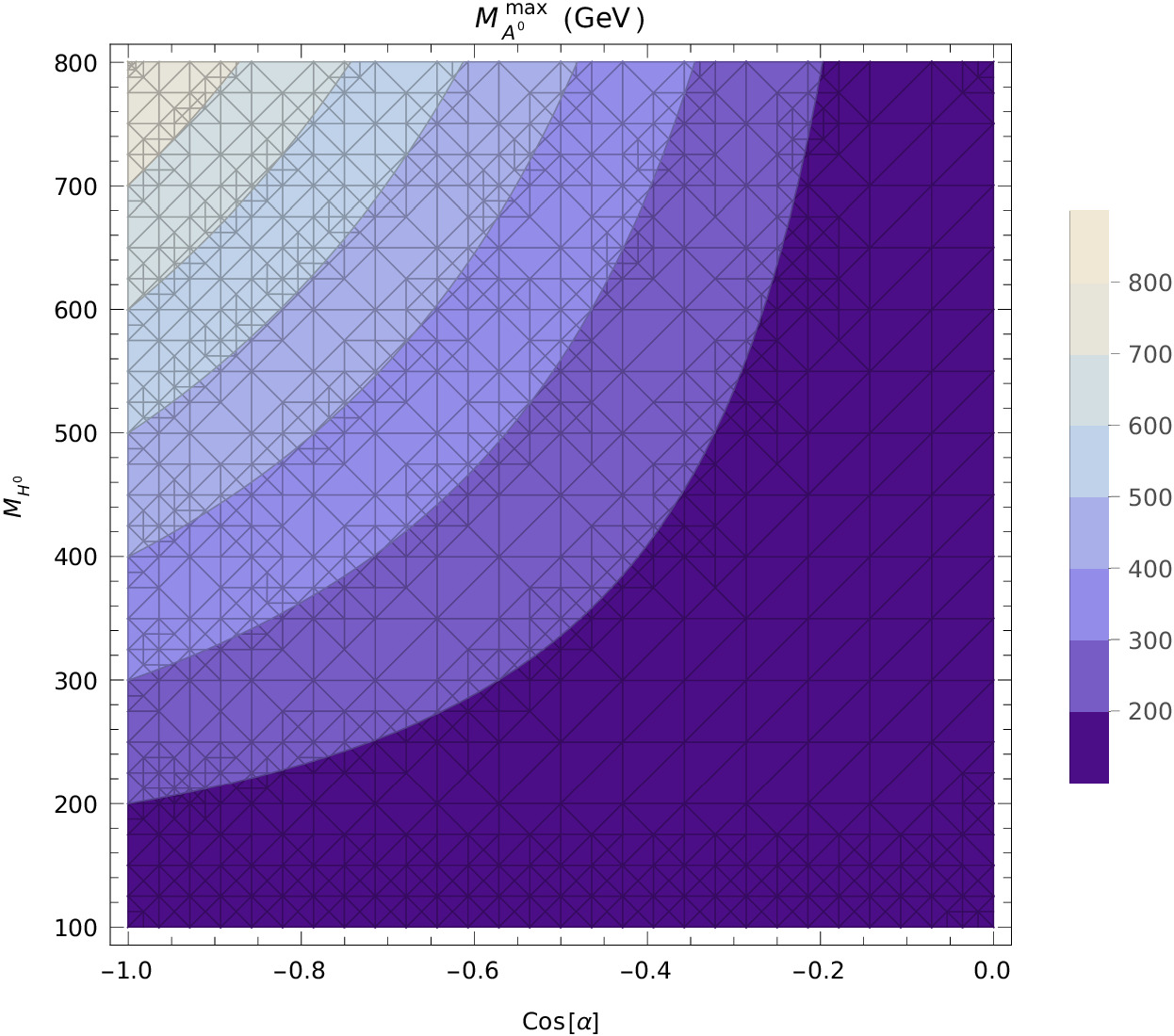
(b)

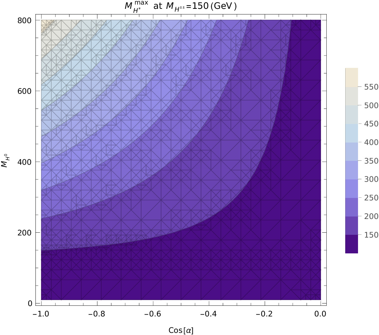
(c)

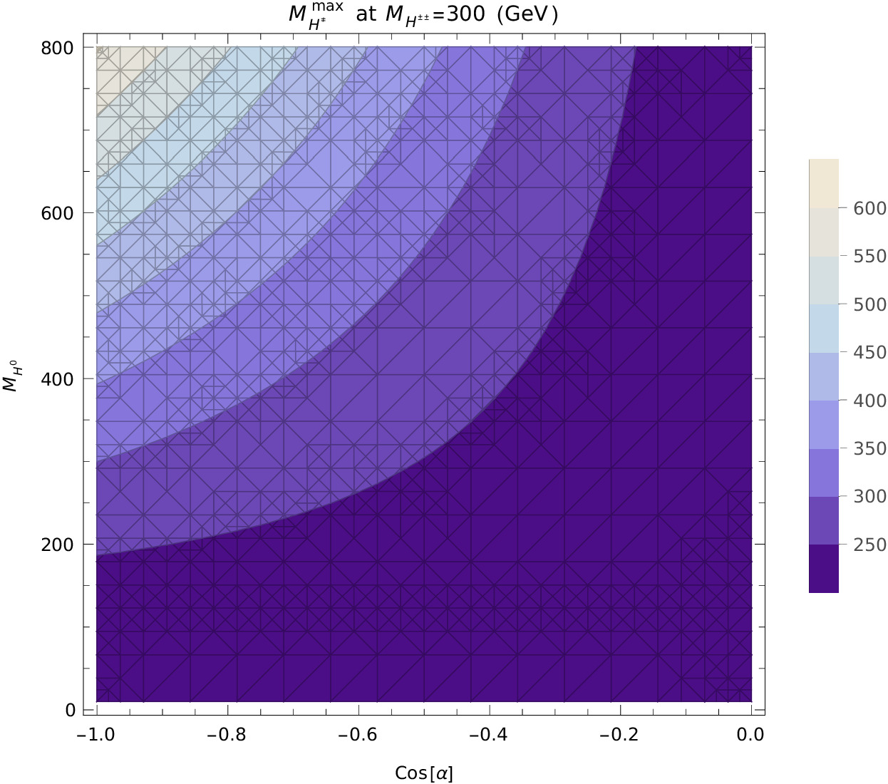
(d)

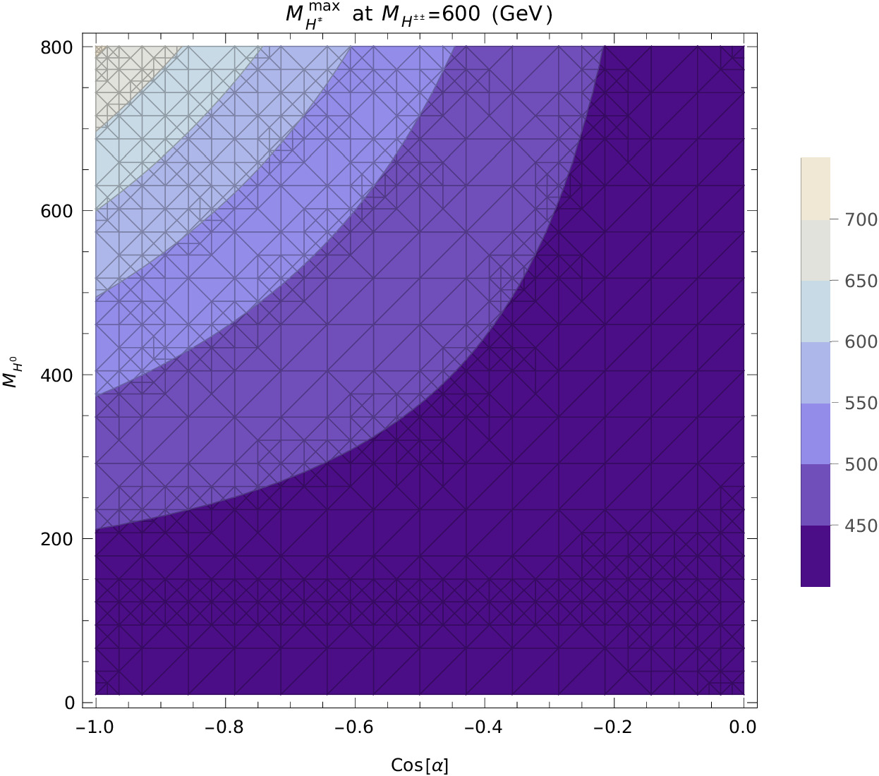
(e)

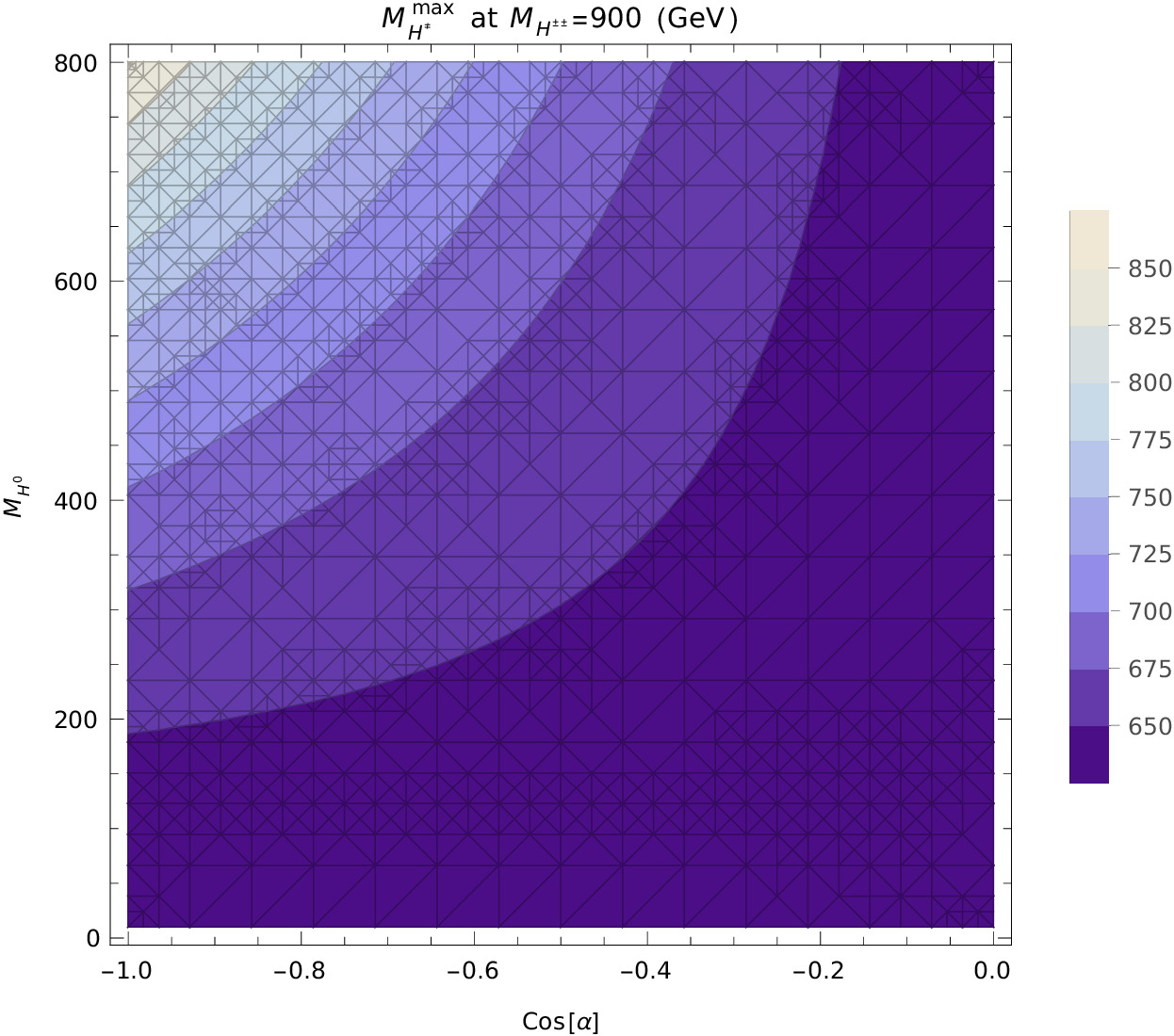
(f)

Figure 11: This figure presents the parameter $\lambda$ (panel (a)), $\mathrm{max}(M_{A^{0}})$ (panel (b)), and $M_{H^{\pm}}$ (panels (c), (d), (e), and (f)) as functions of $M_{H^{0}}$ and $\cos{\alpha}\in[-1,0)$, with $M_{h^{0}}=125\,\mathrm{GeV}$.

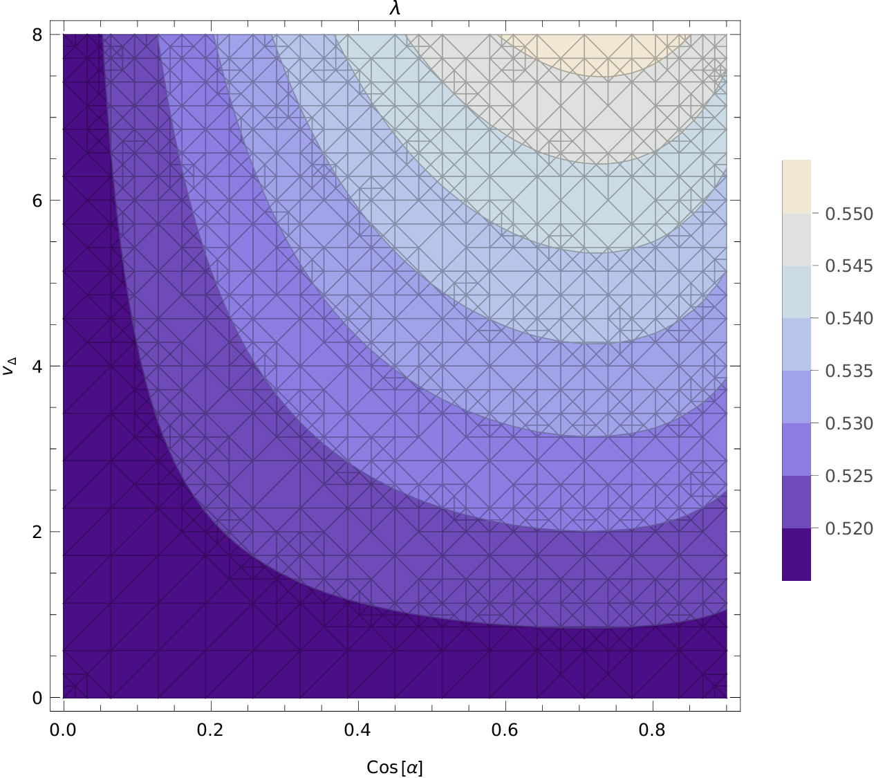
(a)

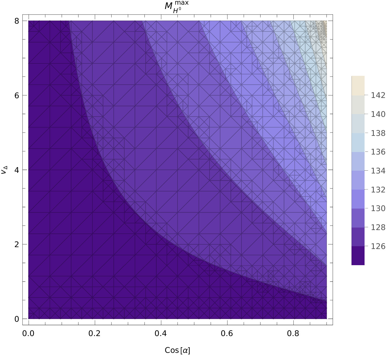
(b)

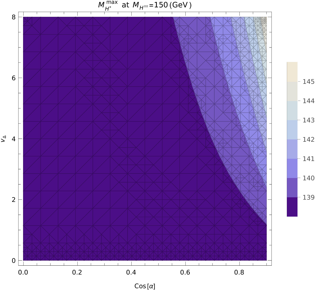
(c)

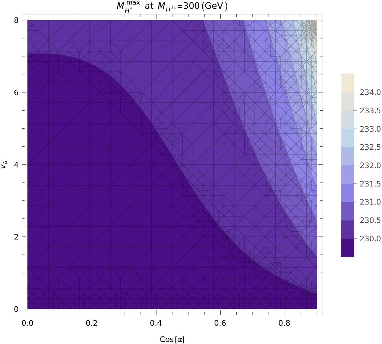
(d)

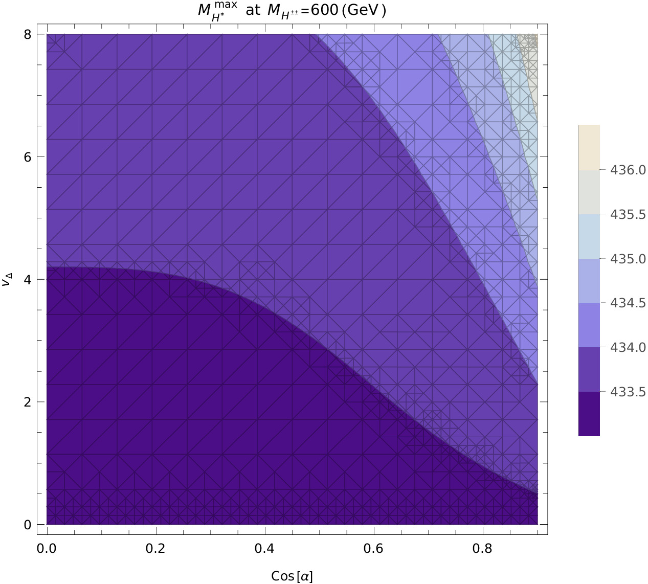
(e)

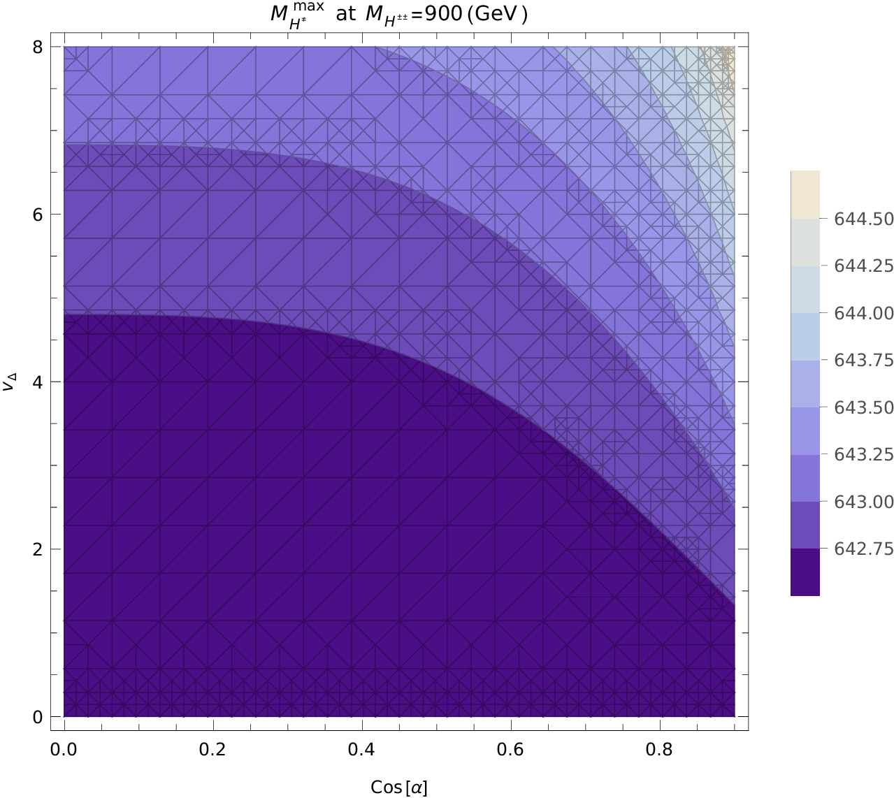
(f)

Figure 12: This figure presents the parameter $\lambda$ (panel (a)), $\mathrm{max}(M_{H^{0}})$ (panel (b)), and $M_{H^{\pm}}$ (panels (c), (d), (e), and (f)) as functions of $M_{h^{0}}$ under scenario II, with $M_{h^{0}}=125\,\mathrm{GeV}$.

References

- Gröber [2017] R. Gröber, Pair Production of Beyond the Standard Model Higgs Bosons, EPJ Web Conf. 164, 05002 (2017), arXiv:1611.07391 [hep-ph] .
- Abouabid et al. [2024] H. Abouabid et al., HHH whitepaper, Eur. Phys. J. C 84, 1183 (2024), arXiv:2407.03015 [hep-ph] .
- Plehn and Rauch [2005] T. Plehn and M. Rauch, The quartic higgs coupling at hadron colliders, Phys. Rev. D 72, 053008 (2005), arXiv:hep-ph/0507321 .
- Baglio et al. [2022] J. Baglio, F. Campanario, S. Glaus, M. M. Mühlleitner, J. Ronca, and M. Spira, Full NLO QCD corrections to Higgs-pair production in the Standard Model and beyond, PoS PANIC2021, 393 (2022).
- Baglio et al. [2021] J. Baglio, F. Campanario, S. Glaus, M. Mühlleitner, J. Ronca, and M. Spira, : Combined uncertainties, Phys. Rev. D 103, 056002 (2021), arXiv:2008.11626 [hep-ph] .
- Biermann et al. [2024] L. Biermann, C. Borschensky, C. Englert, M. Mühlleitner, and W. Naskar, Double and triple Higgs boson production to probe the electroweak phase transition, Phys. Rev. D 110, 095012 (2024), arXiv:2408.08043 [hep-ph] .
- Goncalves et al. [2018] D. Goncalves, T. Han, and S. Mukhopadhyay, Off-Shell Higgs Probe of Naturalness, Phys. Rev. Lett. 120, 111801 (2018), [Erratum: Phys.Rev.Lett. 121, 079902 (2018)], arXiv:1710.02149 [hep-ph] .
- Karkout et al. [2024] O. Karkout, A. Papaefstathiou, M. Postma, G. Tetlalmatzi-Xolocotzi, J. van de Vis, and T. du Pree, Triple Higgs boson production and electroweak phase transition in the two-real-singlet model, JHEP 11, 077, arXiv:2404.12425 [hep-ph] .
- Dawson et al. [2022] S. Dawson et al., Report of the Topical Group on Higgs Physics for Snowmass 2021: The Case for Precision Higgs Physics, in Snowmass 2021 (2022) arXiv:2209.07510 [hep-ph] .
- Lewis et al. [2024] I. M. Lewis, J. Scott, M. A. S. Alcaraz, and M. Sullivan, Real Singlet Scalar Benchmarks in the Multi-TeV Resonance Regime, (2024), arXiv:2410.08275 [hep-ph] .
- de Florian et al. [2020] D. de Florian, I. Fabre, and J. Mazzitelli, Triple Higgs production at hadron colliders at NNLO in QCD, JHEP 03, 155, arXiv:1912.02760 [hep-ph] .
- Bahl et al. [2022] H. Bahl, J. Braathen, and G. Weiglein, New Constraints on Extended Higgs Sectors from the Trilinear Higgs Coupling, Phys. Rev. Lett. 129, 231802 (2022), arXiv:2202.03453 [hep-ph] .
- Plehn et al. [1996] T. Plehn, M. Spira, and P. M. Zerwas, Pair production of neutral Higgs particles in gluon-gluon collisions, Nucl. Phys. B 479, 46 (1996), [Erratum: Nucl.Phys.B 531, 655–655 (1998)], arXiv:hep-ph/9603205 .
- Chiesa et al. [2020] M. Chiesa, F. Maltoni, L. Mantani, B. Mele, F. Piccinini, and X. Zhao, Measuring the quartic Higgs self-coupling at a multi-TeV muon collider, JHEP 09, 098, arXiv:2003.13628 [hep-ph] .
- Arhrib et al. [2014] A. Arhrib, R. Benbrik, G. Moultaka, and L. Rahili, Type II Seesaw Higgsology and LEP/LHC constraints, (2014), arXiv:1411.5645 [hep-ph] .
- Shao et al. [2013] D. Y. Shao, C. S. Li, H. T. Li, and J. Wang, Threshold resummation effects in Higgs boson pair production at the LHC, JHEP 07, 169, arXiv:1301.1245 [hep-ph] .
- de Florian and Mazzitelli [2015] D. de Florian and J. Mazzitelli, Higgs pair production at next-to-next-to-leading logarithmic accuracy at the LHC, JHEP 09, 053, arXiv:1505.07122 [hep-ph] .
- de Florian et al. [2016] D. de Florian et al. (LHC Higgs Cross Section Working Group), Handbook of LHC Higgs Cross Sections: 4. Deciphering the Nature of the Higgs Sector 2/2017, 10.23731/CYRM-2017-002 (2016), arXiv:1610.07922 [hep-ph] .
- Asakawa et al. [2009] E. Asakawa, D. Harada, S. Kanemura, Y. Okada, and K. Tsumura, Higgs boson pair production at a photon-photon collision in the two Higgs doublet model, Phys. Lett. B 672, 354 (2009), arXiv:0809.0094 [hep-ph] .
- Papaefstathiou and Sakurai [2016] A. Papaefstathiou and K. Sakurai, Triple Higgs boson production at a 100 TeV proton-proton collider, JHEP 02, 006, arXiv:1508.06524 [hep-ph] .
- Binoth et al. [2006] T. Binoth, S. Karg, N. Kauer, and R. Ruckl, Multi-Higgs boson production in the Standard Model and beyond, Phys. Rev. D 74, 113008 (2006), arXiv:hep-ph/0608057 .
- Acar et al. [2017] Y. C. Acar, A. N. Akay, S. Beser, A. C. Canbay, H. Karadeniz, U. Kaya, B. B. Oner, and S. Sultansoy, Future circular collider based lepton–hadron and photon–hadron colliders: Luminosity and physics, Nucl. Instrum. Meth. A 871, 47 (2017), arXiv:1608.02190 [physics.acc-ph] .
- Murayama and Peskin [1996] H. Murayama and M. E. Peskin, Physics opportunities of e+ e- linear colliders, Ann. Rev. Nucl. Part. Sci. 46, 533 (1996), arXiv:hep-ex/9606003 .
- Benedikt et al. [2022] M. Benedikt et al., Future Circular Hadron Collider FCC-hh: Overview and Status, (2022), arXiv:2203.07804 [physics.acc-ph] .
- Abada et al. [2019] A. Abada et al. (FCC), FCC-ee: The Lepton Collider: Future Circular Collider Conceptual Design Report Volume 2, Eur. Phys. J. ST 228, 261 (2019).
- Telnov [2006] V. I. Telnov, Photon colliders: The First 25 years, Acta Phys. Polon. B 37, 633 (2006), arXiv:physics/0602172 .
- Arhrib et al. [2009] A. Arhrib, R. Benbrik, C.-H. Chen, and R. Santos, Neutral Higgs boson pair production in photon-photon annihilation in the Two Higgs Doublet Model, Phys. Rev. D 80, 015010 (2009), arXiv:0901.3380 [hep-ph] .
- Delahaye et al. [2019] J. P. Delahaye, M. Diemoz, K. Long, B. Mansoulié, N. Pastrone, L. Rivkin, D. Schulte, A. Skrinsky, and A. Wulzer, Muon Colliders (2019), arXiv:1901.06150 [physics.acc-ph] .
- Palmer [2014] R. B. Palmer, Muon Colliders, Rev. Accel. Sci. Tech. 7, 137 (2014).
- Long et al. [2021] K. Long, D. Lucchesi, M. Palmer, N. Pastrone, D. Schulte, and V. Shiltsev, Muon colliders to expand frontiers of particle physics, Nature Phys. 17, 289 (2021), arXiv:2007.15684 [physics.acc-ph] .
- von Weizsacker [1934] C. F. von Weizsacker, Radiation emitted in collisions of very fast electrons, Z. Phys. 88, 612 (1934).
- Chiesa et al. [2024] M. Chiesa, B. Mele, and F. Piccinini, Multi Higgs production via photon fusion at future multi-TeV muon colliders, Eur. Phys. J. C 84, 543 (2024), arXiv:2109.10109 [hep-ph] .
- Williams [1934a] E. J. Williams, Nature of the high-energy particles of penetrating radiation and status of ionization and radiation formulae, Phys. Rev. 45, 729 (1934a).
- Costantini et al. [2020] A. Costantini, F. De Lillo, F. Maltoni, L. Mantani, O. Mattelaer, R. Ruiz, and X. Zhao, Vector boson fusion at multi-TeV muon colliders, JHEP 09, 080, arXiv:2005.10289 [hep-ph] .
- Al Ali et al. [2022] H. Al Ali et al., The muon Smasher’s guide, Rept. Prog. Phys. 85, 084201 (2022), arXiv:2103.14043 [hep-ph] .
- Black et al. [2024] K. M. Black et al., Muon Collider Forum report, JINST 19 (02), T02015, arXiv:2209.01318 [hep-ex] .
- de Blas et al. [2022] J. de Blas et al. (Muon Collider), The physics case of a 3 TeV muon collider stage, (2022), arXiv:2203.07261 [hep-ph] .
- Capdevilla et al. [2024a] R. Capdevilla, F. Garosi, D. Marzocca, and B. Stechauner, Testing the Neutrino Content of the Muon at Muon Colliders, (2024a), arXiv:2410.21383 [hep-ph] .
- Capdevilla et al. [2021] R. Capdevilla, D. Curtin, Y. Kahn, and G. Krnjaic, Discovering the physics of at future muon colliders, Phys. Rev. D 103, 075028 (2021), arXiv:2006.16277 [hep-ph] .
- Capdevilla et al. [2024b] R. Capdevilla, F. Meloni, and J. Zurita, Discovering Electroweak Interacting Dark Matter at Muon Colliders using Soft Tracks, (2024b), arXiv:2405.08858 [hep-ph] .
- Han et al. [2021a] T. Han, D. Liu, I. Low, and X. Wang, Electroweak couplings of the Higgs boson at a multi-TeV muon collider, Phys. Rev. D 103, 013002 (2021a), arXiv:2008.12204 [hep-ph] .
- Capdevilla et al. [2022] R. Capdevilla, D. Curtin, Y. Kahn, and G. Krnjaic, No-lose theorem for discovering the new physics of at muon colliders, Phys. Rev. D 105, 015028 (2022), arXiv:2101.10334 [hep-ph] .
- Phan et al. [2024a] K. H. Phan, D. T. Tran, and T. H. Nguyen, Processes in Inert Higgs Doublet Models and Two Higgs Doublet Models, (2024a), arXiv:2409.00662 [hep-ph] .
- Phan et al. [2024b] K. H. Phan, D. T. Tran, and T. H. Nguyen, One-loop analytical expressions for in Higgs Extensions of the Standard Models and its applications, (2024b), arXiv:2410.06827 [hep-ph] .
- Figy and Zwicky [2011] T. Figy and R. Zwicky, The other Higgses, at resonance, in the Lee-Wick extension of the Standard Model, JHEP 10, 145, arXiv:1108.3765 [hep-ph] .
- Demirci and Ahmadov [2016] M. Demirci and A. I. Ahmadov, Neutralino pair production via photon-photon collisions at the ILC, Phys. Rev. D 94, 075025 (2016), arXiv:1610.09398 [hep-ph] .
- Demirci [2019] M. Demirci, Pseudoscalar Higgs boson pair production at a photon-photon collision in the two Higgs doublet model, Turk. J. Phys. 43, 442 (2019), arXiv:1902.07236 [hep-ph] .
- Muhlleitner et al. [2001] M. M. Muhlleitner, M. Kramer, M. Spira, and P. M. Zerwas, Production of MSSM Higgs bosons in photon-photon collisions, Phys. Lett. B 508, 311 (2001), arXiv:hep-ph/0101083 .
- Arbabifar et al. [2013] F. Arbabifar, S. Bahrami, and M. Frank, Neutral Higgs Bosons in the Higgs Triplet Model with nontrivial mixing, Phys. Rev. D 87, 015020 (2013), arXiv:1211.6797 [hep-ph] .
- Demirci [2020] M. Demirci, Precise predictions for charged Higgs boson pair production in photon-photon collisions, Nucl. Phys. B 961, 115235 (2020), arXiv:2004.08834 [hep-ph] .
- El Kaffas et al. [2007] A. W. El Kaffas, O. M. Ogreid, and P. Osland, Profile of two-Higgs-doublet-model parameter space, eConf C0705302, HIG08 (2007), arXiv:0709.4203 [hep-ph] .
- Wahab El Kaffas et al. [2007] A. Wahab El Kaffas, P. Osland, and O. M. Ogreid, Constraining the Two-Higgs-Doublet-Model parameter space, Phys. Rev. D 76, 095001 (2007), arXiv:0706.2997 [hep-ph] .
- Higgs [1964] P. W. Higgs, Broken Symmetries and the Masses of Gauge Bosons, Phys. Rev. Lett. 13, 508 (1964).
- Papaefstathiou et al. [2021] A. Papaefstathiou, T. Robens, and G. Tetlalmatzi-Xolocotzi, Triple Higgs Boson Production at the Large Hadron Collider with Two Real Singlet Scalars, JHEP 05, 193, arXiv:2101.00037 [hep-ph] .
- Tumasyan et al. [2022] A. Tumasyan et al. (CMS), A portrait of the Higgs boson by the CMS experiment ten years after the discovery., Nature 607, 60 (2022), [Erratum: Nature 623, (2023)], arXiv:2207.00043 [hep-ex] .
- Chatrchyan et al. [2012] S. Chatrchyan et al. (CMS), Observation of a New Boson at a Mass of 125 GeV with the CMS Experiment at the LHC, Phys. Lett. B 716, 30 (2012), arXiv:1207.7235 [hep-ex] .
- Bhupal Dev et al. [2013] P. S. Bhupal Dev, D. K. Ghosh, N. Okada, and I. Saha, 125 GeV Higgs Boson and the Type-II Seesaw Model, JHEP 03, 150, [Erratum: JHEP 05, 049 (2013)], arXiv:1301.3453 [hep-ph] .
- Kraus et al. [2005] C. Kraus et al., Final results from phase II of the Mainz neutrino mass search in tritium beta decay, Eur. Phys. J. C 40, 447 (2005), arXiv:hep-ex/0412056 .
- Weinheimer et al. [1999] C. Weinheimer, B. Degenddag, A. Bleile, J. Bonn, L. Bornschein, O. Kazachenko, A. Kovalik, and E. W. Otten, High precision measurement of the tritium spectrum near its endpoint and upper limit on the neutrino mass, Phys. Lett. B 460, 219 (1999), [Erratum: Phys.Lett.B 464, 352–352 (1999)].
- Lobashev et al. [2001] V. M. Lobashev et al., Direct Search For Neutrino Mass And Anomaly In The Tritium Beta-spectrum, in 35th Rencontres de Moriond: Electroweak Interactions and Unified Theories (The Gioi, Hanoi, 2001) pp. 45–50.
- Belesev et al. [1995] A. I. Belesev, A. I. Bleule, E. V. Geraskin, A. Golubev, N. Golubev, O. V. Kazachenko, E. P. Kiev, Y. Kuznetsov, V. M. Lobashev, B. M. Ovchinnikov, V. I. Parfenov, I. V. Sekachev, A. P. Solodukhin, N. A. Titov, I. E. Yarykin, Y. I. Zakharov, S. N. Balashov, and P. E. Spivak, Results of the troitsk experiment on the search for the electron antineutrino rest mass in tritium beta-decay, Physics Letters B 350, 263 (1995).
- Aker et al. [2022] M. Aker et al. (KATRIN), Direct neutrino-mass measurement with sub-electronvolt sensitivity, Nature Phys. 18, 160 (2022), arXiv:2105.08533 [hep-ex] .
- Drexlin et al. [2013] G. Drexlin, V. Hannen, S. Mertens, and C. Weinheimer, Current direct neutrino mass experiments, Adv. High Energy Phys. 2013, 293986 (2013), arXiv:1307.0101 [physics.ins-det] .
- Aker et al. [2019] M. Aker et al. (KATRIN), Improved Upper Limit on the Neutrino Mass from a Direct Kinematic Method by KATRIN, Phys. Rev. Lett. 123, 221802 (2019), arXiv:1909.06048 [hep-ex] .
- Schechter and Valle [1980a] J. Schechter and J. W. F. Valle, Neutrino Masses in SU(2) x U(1) Theories, Phys. Rev. D 22, 2227 (1980a).
- Primulando et al. [2019] R. Primulando, J. Julio, and P. Uttayarat, Scalar phenomenology in type-II seesaw model, JHEP 08, 024, arXiv:1903.02493 [hep-ph] .
- Arhrib et al. [2011] A. Arhrib, R. Benbrik, M. Chabab, G. Moultaka, M. C. Peyranere, L. Rahili, and J. Ramadan, The Higgs Potential in the Type II Seesaw Model, Phys. Rev. D 84, 095005 (2011), arXiv:1105.1925 [hep-ph] .
- Rahili et al. [2019] L. Rahili, A. Arhrib, and R. Benbrik, Associated production of SM Higgs with a photon in type-II seesaw models at the ILC, Eur. Phys. J. C 79, 940 (2019), arXiv:1909.07793 [hep-ph] .
- Schechter and Valle [1980b] J. Schechter and J. W. F. Valle, Neutrino masses in su(2) u(1) theories, Phys. Rev. D 22, 2227 (1980b).
- Schechter and Valle [1982] J. Schechter and J. W. F. Valle, Neutrinoless double- decay in su(2)×u(1) theories, Phys. Rev. D 25, 2951 (1982).
- Babu et al. [2017] K. S. Babu, I. Gogoladze, and S. Khan, Radiative Electroweak Symmetry Breaking in Standard Model Extensions, Phys. Rev. D 95, 095013 (2017), arXiv:1612.05185 [hep-ph] .
- Du et al. [2019] Y. Du, A. Dunbrack, M. J. Ramsey-Musolf, and J.-H. Yu, Type-II Seesaw Scalar Triplet Model at a 100 TeV Collider: Discovery and Higgs Portal Coupling Determination, JHEP 01, 101, arXiv:1810.09450 [hep-ph] .
- Akeroyd and Moretti [2012a] A. G. Akeroyd and S. Moretti, Enhancement of H to gamma gamma from doubly charged scalars in the Higgs Triplet Model, Phys. Rev. D 86, 035015 (2012a), arXiv:1206.0535 [hep-ph] .
- Akeroyd and Moretti [2012b] A. G. Akeroyd and S. Moretti, Enhancement of from charged Higgs bosons in the Higgs Triplet Model, PoS CHARGED2012, 035 (2012b), arXiv:1210.6882 [hep-ph] .
- Akeroyd and Moretti [2011] A. G. Akeroyd and S. Moretti, Production of doubly charged scalars from the decay of a heavy SM-like Higgs boson in the Higgs Triplet Model, Phys. Rev. D 84, 035028 (2011), arXiv:1106.3427 [hep-ph] .
- Akeroyd and Chiang [2010] A. G. Akeroyd and C.-W. Chiang, Phenomenology of Large Mixing for the CP-even Neutral Scalars of the Higgs Triplet Model, Phys. Rev. D 81, 115007 (2010), arXiv:1003.3724 [hep-ph] .
- Ashanujjaman and Ghosh [2022] S. Ashanujjaman and K. Ghosh, Revisiting type-II see-saw: present limits and future prospects at LHC, JHEP 03, 195, arXiv:2108.10952 [hep-ph] .
- Aoki et al. [2012] M. Aoki, S. Kanemura, M. Kikuchi, and K. Yagyu, Renormalization of the Higgs Sector in the Triplet Model, Phys. Lett. B 714, 279 (2012), arXiv:1204.1951 [hep-ph] .
- Das and Santamaria [2016] D. Das and A. Santamaria, Updated scalar sector constraints in the Higgs triplet model, Phys. Rev. D 94, 015015 (2016), arXiv:1604.08099 [hep-ph] .
- Samarakoon and Figy [2024] B. Samarakoon and T. M. Figy, Double Higgs boson production via photon fusion at muon colliders within the triplet Higgs model, Phys. Rev. D 109, 075015 (2024), arXiv:2312.12594 [hep-ph] .
- Ducu et al. [2024] O. A. Ducu, A. E. Dumitriu, A. Jinaru, R. Kukla, E. Monnier, G. Moultaka, A. Tudorache, and H. Xu, Type-II Seesaw Higgs triplet productions and decays at the LHC, (2024), arXiv:2410.14830 [hep-ph] .
- Christensen and Duhr [2009] N. D. Christensen and C. Duhr, FeynRules - Feynman rules made easy, Comput. Phys. Commun. 180, 1614 (2009), arXiv:0806.4194 [hep-ph] .
- Alloul et al. [2014] A. Alloul, N. D. Christensen, C. Degrande, C. Duhr, and B. Fuks, FeynRules 2.0 - A complete toolbox for tree-level phenomenology, Comput. Phys. Commun. 185, 2250 (2014), arXiv:1310.1921 [hep-ph] .
- Hahn and Perez-Victoria [1999] T. Hahn and M. Perez-Victoria, Automatized one loop calculations in four-dimensions and D-dimensions, Comput. Phys. Commun. 118, 153 (1999), arXiv:hep-ph/9807565 .
- Denner [1993] A. Denner, Techniques for calculation of electroweak radiative corrections at the one loop level and results for W physics at LEP-200, Fortsch. Phys. 41, 307 (1993), arXiv:0709.1075 [hep-ph] .
- Hahn [2016] T. Hahn, Concurrent Cuba, Comput. Phys. Commun. 207, 341 (2016).
- Hahn [2005] T. Hahn, CUBA: A Library for multidimensional numerical integration, Comput. Phys. Commun. 168, 78 (2005), arXiv:hep-ph/0404043 .
- Hahn [2001] T. Hahn, Generating Feynman diagrams and amplitudes with FeynArts 3, Comput. Phys. Commun. 140, 418 (2001), arXiv:hep-ph/0012260 .
- Nogueira [1993] P. Nogueira, Automatic Feynman Graph Generation, J. Comput. Phys. 105, 279 (1993).
- Vermaseren [2000] J. A. M. Vermaseren, New features of FORM, (2000), arXiv:math-ph/0010025 .
- Cullen et al. [2011a] G. Cullen, M. Koch-Janusz, and T. Reiter, Spinney: A Form Library for Helicity Spinors, Comput. Phys. Commun. 182, 2368 (2011a), arXiv:1008.0803 [hep-ph] .
- Reiter [2010] T. Reiter, Optimising Code Generation with haggies, Comput. Phys. Commun. 181, 1301 (2010), arXiv:0907.3714 [hep-ph] .
- Mastrolia et al. [2010] P. Mastrolia, G. Ossola, T. Reiter, and F. Tramontano, Scattering AMplitudes from Unitarity-based Reduction Algorithm at the Integrand-level, JHEP 08, 080, arXiv:1006.0710 [hep-ph] .
- Binoth et al. [2009] T. Binoth, J. P. Guillet, G. Heinrich, E. Pilon, and T. Reiter, Golem95: A Numerical program to calculate one-loop tensor integrals with up to six external legs, Comput. Phys. Commun. 180, 2317 (2009), arXiv:0810.0992 [hep-ph] .
- Cullen et al. [2011b] G. Cullen, J. P. Guillet, G. Heinrich, T. Kleinschmidt, E. Pilon, T. Reiter, and M. Rodgers, Golem95C: A library for one-loop integrals with complex masses, Comput. Phys. Commun. 182, 2276 (2011b), arXiv:1101.5595 [hep-ph] .
- Guillet et al. [2014] J. P. Guillet, G. Heinrich, and J. F. von Soden-Fraunhofen, Tools for NLO automation: extension of the golem95C integral library, Comput. Phys. Commun. 185, 1828 (2014), arXiv:1312.3887 [hep-ph] .
- van Deurzen et al. [2014] H. van Deurzen, G. Luisoni, P. Mastrolia, E. Mirabella, G. Ossola, and T. Peraro, Multi-leg One-loop Massive Amplitudes from Integrand Reduction via Laurent Expansion, JHEP 03, 115, arXiv:1312.6678 [hep-ph] .
- Peraro [2014] T. Peraro, Ninja: Automated Integrand Reduction via Laurent Expansion for One-Loop Amplitudes, Comput. Phys. Commun. 185, 2771 (2014), arXiv:1403.1229 [hep-ph] .
- Cullen et al. [2014] G. Cullen et al. (GoSam), GS-2.0: a tool for automated one-loop calculations within the Standard Model and beyond, Eur. Phys. J. C 74, 3001 (2014), arXiv:1404.7096 [hep-ph] .
- Kleiss et al. [1986] R. Kleiss, W. J. Stirling, and S. D. Ellis, A New Monte Carlo Treatment of Multiparticle Phase Space at High-energies, Comput. Phys. Commun. 40, 359 (1986).
- Plätzer [2013] S. Plätzer, RAMBO on diet, (2013), arXiv:1308.2922 [hep-ph] .
- Campbell et al. [2018] J. Campbell, J. Huston, and F. Krauss, The Black Book of Quantum Chromodynamics : a Primer for the LHC Era (Oxford University Press, 2018).
- Weizsäcker [1934] C. F. V. Weizsäcker, Ausstrahlung bei Stößen sehr schneller Elektronen, Zeitschrift fur Physik 88, 612 (1934).
- Williams [1934b] E. J. Williams, Nature of the high energy particles of penetrating radiation and status of ionization and radiation formulae, Phys. Rev. 45, 729 (1934b).
- Landau and Lifschitz [1934] L. D. Landau and E. M. Lifschitz, ON THE PRODUCTION OF ELECTRONS AND POSITRONS BY A COLLISION OF TWO PARTICLES, Phys. Z. Sowjetunion 6, 244 (1934).
- Garosi et al. [2023] F. Garosi, D. Marzocca, and S. Trifinopoulos, LePDF: Standard Model PDFs for high-energy lepton colliders, JHEP 09, 107, arXiv:2303.16964 [hep-ph] .
- Han et al. [2021b] T. Han, Y. Ma, and K. Xie, High energy leptonic collisions and electroweak parton distribution functions, Phys. Rev. D 103, L031301 (2021b), arXiv:2007.14300 [hep-ph] .
- Han et al. [2022] T. Han, Y. Ma, and K. Xie, Quark and gluon contents of a lepton at high energies, JHEP 02, 154, arXiv:2103.09844 [hep-ph] .
- Schwartz [2014] M. D. Schwartz, Quantum Field Theory and the Standard Model (Cambridge University Press, 2014).
- Haber [2013] H. E. Haber, The Higgs data and the Decoupling Limit, in 1st Toyama International Workshop on Higgs as a Probe of New Physics 2013 (2013) arXiv:1401.0152 [hep-ph] .
- Plehn [2012] T. Plehn, Lectures on LHC Physics, Lect. Notes Phys. 844, 1 (2012), arXiv:0910.4182 [hep-ph] .