IDEA Prune: An Integrated Enlarge-and-Prune Pipeline in Generative Language Model Pretraining

Abstract

Recent advancements in large language models have intensified the need for efficient and deployable models within limited inference budgets. Structured pruning pipelines have shown promise in token efficiency compared to training target-size models from scratch. In this paper, we advocate incorporating enlarged model pretraining, which is often ignored in previous works, into pruning. We study the enlarge-and-prune pipeline as an integrated system to address two critical questions: whether it is worth pretraining an enlarged model even when the model is never deployed, and how to optimize the entire pipeline for better pruned models. We propose an integrated enlarge-and-prune pipeline, which combines enlarge model training, pruning, and recovery under a single cosine annealing learning rate schedule. This approach is further complemented by a novel iterative structured pruning method for gradual parameter removal. The proposed method helps to mitigate the knowledge loss caused by the rising learning rate in naive enlarge-and-prune pipelines and enable effective redistribution of model capacity among surviving neurons, facilitating smooth compression and enhanced performance. We conduct comprehensive experiments on compressing 2.8B models to 1.3B with up to 2T tokens in pretraining. It demonstrates the integrated approach not only provides insights into the token efficiency of enlarged model pretraining but also achieves superior performance of pruned models.

1 Introduction

Recent advances in large language models have empirically validated the scaling law (Kaplan et al., 2020; Hoffmann et al., 2022), demonstrating that increased model size yields predictable improvements in performance. This insight has driven a race toward larger models, as evidenced by recent developments (Jiang et al., 2024; Dubey et al., 2024). However, the deployment of such models in practical applications faces significant hardware constraints, particularly in terms of inference latency and memory requirements. For example, on-device deployments typically restrict models to 3 billion parameters (Abdin et al., 2024; Gunter et al., 2024). This tension between scaling up models and hardware constraints highlights a critical research challenge: how can we improve model capabilities while maintaining a target model size budget?

Structured pruning pipelines (Xia et al., 2022; Wang et al., 2019; Kwon et al., 2022) offer a promising approach through a two-stage process of pruning and recovery. The pruning stage compresses an enlarged model to the target size through parameter removal, followed by a recovery stage that restores the model’s performance through continual pretraining. This two-stage pipeline offers significant token efficiency: the pruned model, benefiting from the knowledge encoded in its pruning-informed initialization, demonstrates superior performance while requiring fewer training tokens compared to conventional training of an equivalent-sized model from random initialization (Xia et al., 2023; Muralidharan et al., 2024).

Despite the token efficiency of pruning and recovery stages, it is necessary to include enlarged model pretraining to the pipeline and rethink of the overall token efficiency. First, this is because enlarged models serve only as an intermediate step in pruning pipelines and are discarded after target-size model deployments. Considering the cost of training the enlarged model, it becomes unclear whether the pruning approach still outperforms simply training the target-sized model from scratch. Second, even if one could find an enlarged model that is deployed, the model size is usually too large (e.g., more than 8B (Liu et al., 2024; Dubey et al., 2024)) to prune it into the target size (e.g., 1B). This excessive dimensional reduction usually results in poor pruned models, as our empirical analysis in Section 5.2 shows that a 300M target model achieves better results when pruned from a 600M model than from a 1B model. This indicates the necessity of building an enlarged model specifically for a target-size model to achieve a better pruned model.

This paper is the first to advocate incorporating enlarged model pretraining into the pruning pipeline, and study them together as a whole, which we call the enlarge-and-prune pipeline. This pipeline helps us understand the token efficiency of the structured pruning and answer the question whether it is necessary to pretrain an enlarged model even if it is never deployed. To this end, our pilot experiments naively prepend enlarged model pretraining to the pruning and compare the naive enlarge-and-prune pipeline against simply training target-size models from scratch given the same training tokens on the same dataset. Figure 1(a) reveals that the naive pipeline fails to consistently achieve superior token efficiency compared to direct pretraining of target-size models. This inefficiency can be attributed primarily to the divided nature of the naive pipeline, where the training processes across successive stages often lack optimal alignment. For example, from the perspective of the learning rate, the initial learning rate in a new stage substantially exceeds the end learning rate of its predecessor, as illustrated in Figure 2(a) and Figure 2(b). This discontinuity triggers a sharp increase in the loss curve, as shown in Figure 1(b), leading to catastrophic forgetting previously acquired knowledge and ultimately degraded model performance. Furthermore, the naive pipeline employs disparate training objectives across stages, such as auxiliary regularization for mask learning (Xia et al., 2023) and activation-based proxy losses (Muralidharan et al., 2024), resulting in suboptimal initialization for the recovery stage.

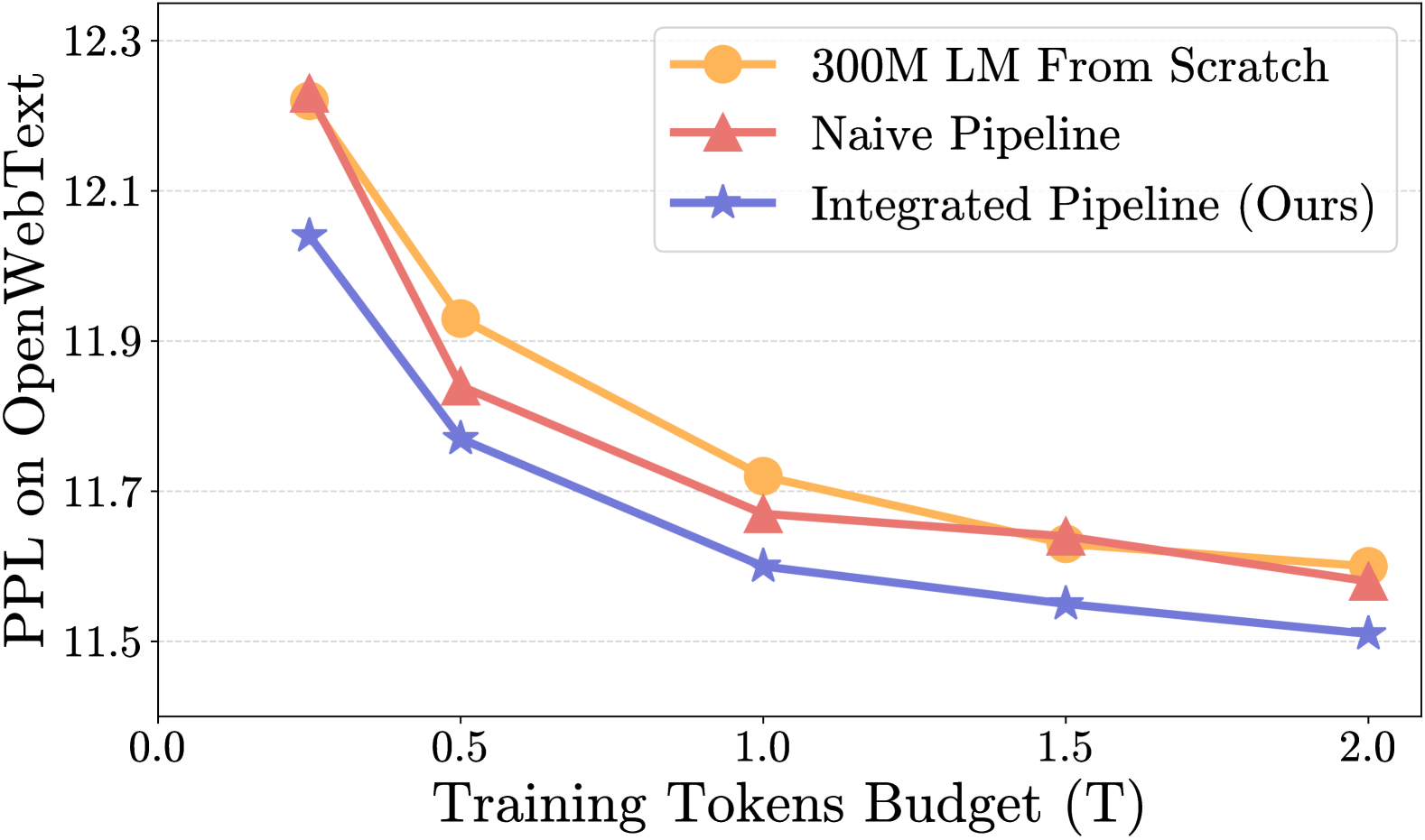
(a) Perplexity on OpenWebText

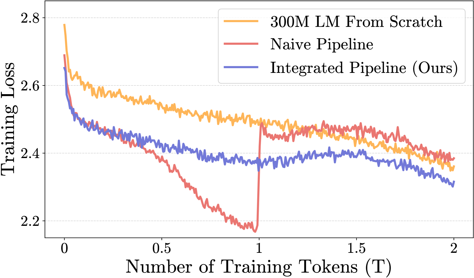
(b) Training Loss

Figure 1: Naive pipeline: 1T for enlarged model training and 1T for pruned model recovery, each with separate learning rate decay. Integrated pipeline: single learning rate schedule matching target-size model training, pruning started at 1T. Left: Perplexity on OpenWebText of 300M model trained with multiple training token budgets from 0.25T to 2T. Right: Training loss curves across enlarge-and-prune pipelines. Training 300M models with 2T total token budget.

To overcome the aforementioned limitations, we propose IDEA Prune, an IntegrateD Enlarge-And-Prune pipeline with a novel iterative structured pruning. The integrated pipeline organically combines the enlarged model pretraining, pruning, and pruned model recovery stages under one cosine annealing learning rate schedule, as illustrated in Figure 2(c). This helps to mitigate the knowledge loss caused by the rising learning rate in naive pipelines (see Figure 1(b)), where each stage uses an individual cosine annealing with warm up (Muralidharan et al., 2024; Xia et al., 2023). Furthermore, we extend iterative pruning (Zhu & Gupta, 2017; Louizos et al., 2017) to structured Feed-Forward Network (FFN) compression. Our approach progressively removes neurons, which corresponds to the rows in weight matrices with the same indices. We identify the surviving neurons based on element-wise importance scores computed across FFN weight matrices (Molchanov et al., 2019; Zhang et al., 2022; Ding et al., 2019). Through iterative width reduction and parameter updates, this approach enables effective redistribution of model capacity among surviving neurons, facilitating smooth compression and enhanced performance.

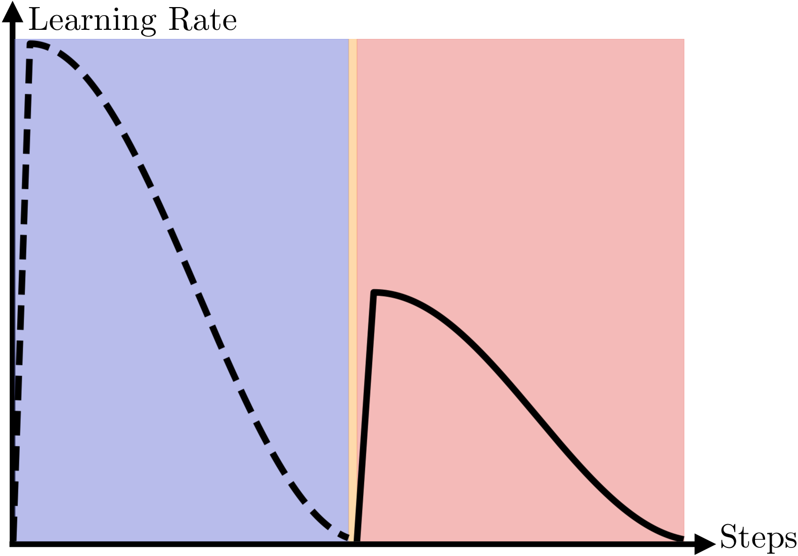
(a) Minitron LR Schedule

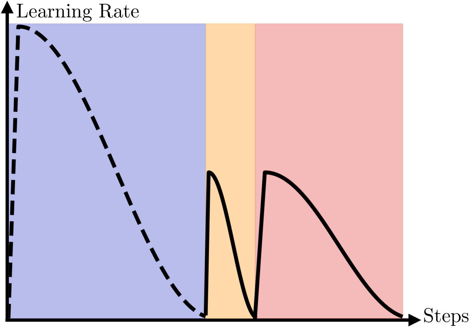
(b) Sheared LLaMA LR Schedule

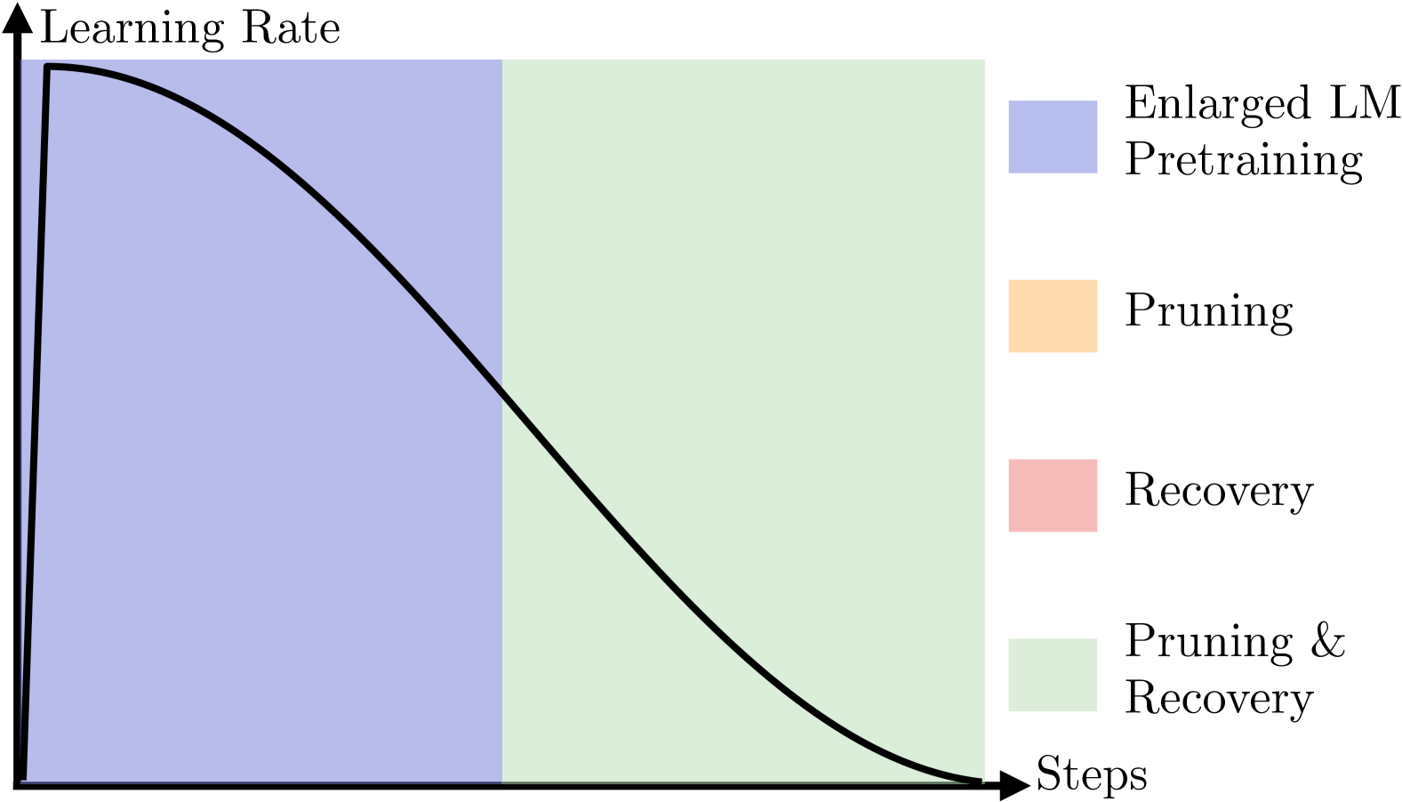
(c) IDEA Prune LR Schedule

Figure 2: Learning rate schedule for separate (Figure 2(a), 2(b)) and integrated (Figure 2(c)) enlarge-and-prune pipelines. Minitron uses single shot pruning, resulting in a narrow pruning stage. Our integrated pipeline uses one single learning rate decay schedule for all stages. We use iterative structured pruning to further integrate pruning and recovery training.

We demonstrate the effectiveness of IDEA Prune through extensive experiments, compressing a 2.8B model to 1.3B parameters with up to 2T training tokens. IDEA Prune extends pruning beyond continual pretraining to the full pretraining regime, further unleashing the power of generative language models. In controlled comparisons with existing approaches—one-shot random pruning, learned mask pruning (Xia et al., 2023), and activation-based pruning (Muralidharan et al., 2024)—our method demonstrates consistent performance improvements across multiple benchmarks. Notably, IDEA Prune significantly improves MMLU accuracy to 46.4%, compared to 31.4-33.4% for baseline methods. In ablation studies, we discover that an intermediate checkpoint, despite showing lower performance than the final checkpoint, provides a more favorable starting point for pruning. We also show the robustness of the hyperparameters in our method, heavily reducing the cost of hyperparameter tuning. For rigorous evaluation of the pruning methodology itself, we isolate our analysis from complementary techniques such as knowledge distillation, though we conduct separate ablation studies to confirm knowledge distillation can be effectively combined with our method for further improvements.

2 Background and Related Work

2.1 Iterative Pruning

Iterative pruning is a parameter reduction technique that alternates between parameter optimization and selective elimination (Zhu & Gupta, 2017; Louizos et al., 2017). During pruning, the method computes importance scores for parameters and gradually removes those less critical. For a model with parameters $\bm{\theta}^{(t)}\in\mathbb{R}^{N}$, we measure parameter importance by sensitivity (Molchanov et al., 2019):

$$\bm{\omega}^{(t)}=\left|\nabla\mathcal{L}(\bm{\theta}^{(t)})\odot\bm{\theta}^{(t)}\right|,$$ (2.1)

where $\mathcal{L}(\cdot)$ is the loss function. This score represents a the first-order approximation of each parameter’s impact on the loss: $\bm{\omega}^{(t)}\approx\left|\mathcal{L}(\bm{\theta}^{(t)})-\mathcal{L}(\bm{\theta}_{-k}^{(t)})\right|$, where $\bm{\theta}_{-k}^{(t)}=\left(\theta_{1},\ldots,\theta_{k-1},0,\theta_{k+1},\ldots,\theta_{N}\right)$. We then generate a binary mask $\bm{v}^{(t)}$ based on the ranking of $\bm{\omega}^{(t)}$, and apply it to obtain the pruned parameters: $\bm{\theta}^{(t)}_{\rm pruned}=\bm{v}^{(t)}\odot\bm{\theta}^{(t)}$. This progressive approach enables smooth transition from larger to smaller models. Note that these works focus on unstructured pruning, while we extend iterative pruning to structured pruning of FFN width in Section 3.2.

2.2 Structured Pruning of FFN

Transformers (Vaswani, 2017), the mainstream architectures in current generative language models (Radford et al., 2019; Jiang et al., 2023; Dubey et al., 2024; Gunter et al., 2024), consist of sequential layers containing attention and Feed-Forward Network (FFN) components. We consider an FFN layer equipped with a gated Sigmoid Linear Unit (SiLU) activation function, denoted as $\sigma(\cdot)$. Given the input $\bm{x}\in\mathbb{R}^{d}$, the layer’s output $\bm{y}\in\mathbb{R}^{d}$ is defined as

$$\bm{y} =\bm{W}_{\rm down}^{\top}(\sigma(\bm{W}_{\rm up}\bm{x})\odot(\bm{W}_{\rm gate}\bm{x}))$$

$$=\sum_{i=1}^{h}\bm{W}_{{\rm down}[i,:]}^{\top}\left((\bm{W}_{{\rm up}[i,:]}x)(\bm{W}_{{\rm gate}[i,:]}\bm{x})\right),$$

where $\bm{W}_{\rm up},\bm{W}_{\rm gate},\bm{W}_{\rm down}\in\mathbb{R}^{h\times d}$, $d$ is the input dimension, $h$ is the hidden dimension or the number of neurons, and $\odot$ represents element-wise multiplication. Structured pruning of FFN width targets the removal of neurons, which corresponds to the rows in $\bm{W}_{\rm up}$, $\bm{W}_{\rm gate}$, and $\bm{W}_{\rm down}$ with the same indices, for example, $\bm{W}_{{\rm up}[i,:]},\bm{W}_{{\rm up}[i,:]},\bm{W}_{{\rm up}[i,:]}$. This is achieved by finding a binary mask $\bm{m}\in\{0,1\}^{h}$ that determines which neurons to retain. The pruned weight matrices are:

$$\begin{split}\bm{W}_{\rm up}^{{}^{\prime}}&={\rm diag}(\bm{m})\times\bm{W}_{\rm up},\\ \bm{W}_{\rm gate}^{{}^{\prime}}&={\rm diag}(\bm{m})\times\bm{W}_{\rm gate},\\ \bm{W}_{\rm down}^{{}^{\prime}}&={\rm diag}(\bm{m})\times\bm{W}_{\rm down}.\end{split}$$ (2.2)

After mask application, the zero columns in each matrix are eliminated to obtain compressed weight matrices, resulting in reduced memory consumption and inference latency.

In this paper, we focus on pruning FFN width. We do not prune the depth as Muralidharan et al. (2024) suggest pruning width (i.e., the hidden dimensions of FFN layers and number of attention heads in attention layers) is more efficient than pruning depth (i.e., the number of transformer layers). Additionally, we exclude attention layers from our pruning, both for simplicity and due to their relatively minor contribution to the total parameters (less than 20%).

2.3 Cosine Annealing Learning Rate Schedule

In pretraining, a gradient-based optimization algorithm (Loshchilov, 2017) is employed to update the model. Specifically, at the $t$-th step, we update the matrix $\bm{W}^{(t-1)}$ from the last step by

$$\bm{W}^{(t)}=\bm{W}^{(t-1)}-\gamma^{(t)}\widetilde{\bm{G}}^{(t)},$$ (2.3)

where $\widetilde{\bm{G}}^{(t)}$ is the smoothed gradient of matrix $\bm{W}^{(t-1)}$ (see Appendix A), and $\gamma^{(t)}$ is the learning rate, which is often scheduled by a cosine annealing with a linear warm-up (Loshchilov & Hutter, 2016). Specifically, given a fixed total number of training steps $T$, the cosine annealing learning rate schedule is

$$\eta(t;T,\eta_{\rm p},\eta_{\rm e})=\begin{cases}\frac{t}{T_{0}}\eta_{p}&\text{if $0<t\leq T_{0}$},\\ c_{1}\cos\left(\frac{t-T_{0}}{T}\pi\right)+c_{2}&\text{if $T_{0}<t\leq T$},\end{cases}$$ (2.4)

where $c_{1}=\frac{1}{2}(\eta_{p}-\eta_{e}),c_{2}=\frac{1}{2}(\eta_{p}+\eta_{e})$, $T_{0}$ represents the number of warmup steps, and $\eta_{p}$ and $\eta_{e}$ are the peak and end learning rates, respectively.

2.4 Naive Enlarge-and-Prune Pipeline

A naive enlarge-and-prune pipeline (Xia et al., 2023; Muralidharan et al., 2024) consists of three distinct stages: enlarged model pretraining, pruning, and pruned model recovery. In the view of learning rate specifically, each of the three stages uses its own independent learning rate schedule (Xia et al., 2023). The learning rate at the $t$-th step through the naive enlarge-and-prune pipeline is

$$\beta^{(t)}=\begin{cases}\eta(t;T_{l},\eta_{1},\eta_{2})&\text{if $0<t\leq T_{l}$},\\ \eta(t-T_{l};T_{p},\eta_{3},\eta_{4})&\text{if $T_{l}<t\leq T_{l}+T_{p}$},\\ \eta(t-T_{l}-T_{p};T_{r},\eta_{5},\eta_{6})&\text{if $T_{l}+T_{p}<t\leq T$},\end{cases}$$

where $T$ is the total training steps and $T_{l},T_{p},T_{r}$ are the number of enlarged model training steps, pruning steps, pruned model recovery steps, respectively. An example can be found in Figure 2(b). In the naive enlarge-and-prune pipeline, we need to tune different sets of peak and end learning rates $\eta_{1},...,\eta_{6}$, which takes a lot of effort to find the optimal learning rate sets.

2.5 Train Large, Then Compress

Li et al. (2020) demonstrate that pretraining larger models with early stopping is computationally more efficient than training smaller models to convergence. To meet test-time constraints, they compress the large model through downstream task adaptation, which outperforms naive pretraining and finetuning of equivalent-sized models.

While this approach shares similarities with our method, there are several key distinctions. Our work employs structured pruning, which maintains inference speeds, whereas their unstructured pruning approach fails to match the latency of similarly-sized dense models due to limited hardware support for sparse matrix operations. Furthermore, we conduct pruning exclusively during pretraining to produce a general-purpose pretrained model, in contrast to their task-specific pruning during finetuning, which leaves the model’s broader applicability unclear. Finally, we focus on decoder-only transformers, while their findings are based on encoder-only architectures like RoBERTa (Liu, 2019)—a significant architectural difference given the disparate pruning behaviors observed in recent works (Xia et al., 2022, 2023).

3 Method

We propose IDEA Prune, an IntegrateD Enlarge-And-Prune pipeline with a novel iterative structured pruning, to obtain models with a target size from scratch. IDEA Prune combines the enlarged model pretraining, pruning, and pruned model recovery into a single training run. It mitigates the performance degradation of the naive enlarge-and-prune pipeline and reduces the cost of learning rate tuning. Moreover, we unify the pruning and recovery stages by iteratively pruning the neurons based on their importance scores, which provides an accurate and smooth pruning to remove redundant neurons, preventing drastic performance drop.

3.1 Integrated Enlarge-and-Prune Pipeline

We denote the number of enlarged model pretraining steps, pruning steps, pruned model recovery steps as $T_{l},T_{p},T_{r}$, respectively. The learning rate for weight matrix update at step $t$ given by

$$\alpha^{(t)}=\eta(t;T_{l}+T_{p}+T_{r},\eta_{p},\eta_{e}),$$

where $\eta(\cdot;\cdot)$ is the cosine annealing learning rate schedule defined in (2.4). Unlike the naive enlarge-and-prune pipeline in Section 2.4, our integrated approach eliminates learning rate warm-up during pruning and recovery stages, thereby mitigating potential knowledge loss.

Critically, this method is not constrained to specific pruning techniques. We ablate its effectiveness across diverse approaches, including one-shot random pruning, activation-based pruning, and learned mask pruning in Section 5.4.

Furthermore, the integrated pipeline offers additional flexibility by enabling application to existing pretrained models with available intermediate checkpoints and historical learning rate schedules, as discussed in Section 5.1.

3.2 Iterative Structured Pruning in FFN

To complement the integrated learning rate schedule, we propose a specialized iterative pruning for FFN width pruning based on the importance score of neurons. This approach further aligns the pruning and recovery stages by mitigating the suboptimal model initialization inherent in separate pipeline approaches during recovery training.

Concretely, for each element in a weight matrix $\bm{W}^{(t)}\in\mathbb{R}^{h\times d}$ at the $t$-th step, we define the importance score as the sensitivity $\bm{S}_{ij}^{(t)}$ defined in (2.1). Since the sensitivity is defined on the full dataset, we use the moving average of importance scores on a mini-batch of size $B$ to approximate it as

$$\widetilde{\bm{S}}_{ij}^{(t)}=(1-\lambda)\bm{T}_{ij}^{(t)}+\lambda\widetilde{\bm{S}}_{ij}^{(t-1)},$$ (3.1)

where

$$\bm{T}_{ij}^{(t)}=\left|\frac{1}{B}\sum_{n=1}^{B}\nabla l_{n}(\bm{W}_{ij}^{(t)})\bm{W}_{ij}^{(t)}\right|,$$

and $l_{n}(\cdot)$ is the loss of the $n$-th sample in the mini-batch. The importance score for the $k$-th neuron is then derived by combining the moving average scores across the three weight matrices $\bm{W}_{{\rm up}},\bm{W}_{{\rm gate}},\bm{W}_{{\rm down}}$:

$$\bm{c}_{k}^{(t)}=f_{2}\left(f_{1}(\widetilde{\bm{S}}_{{\rm up}[k,:]}^{(t)}),f_{1}(\widetilde{\bm{S}}_{{\rm gate}[k,:]}^{(t)}),f_{1}(\widetilde{\bm{S}}_{{\rm down}[k,:]}^{(t)})\right),$$ (3.2)

where $f_{1}:\mathbb{R}^{d}\rightarrow\mathbb{R}$ and $f_{2}:\mathbb{R}^{3}\rightarrow\mathbb{R}$ are combination functions, such as $\max(\cdot),{\rm mean}(\cdot)$. Finally, we update the pruning mask using a scheduled sparsity by

$$\bm{m}_{k}^{(t)}=\begin{cases}1&\text{if $\bm{c}_{k}^{(t)}$ is in top $r(t;T_{p})$ of $\bm{c}^{(t)}$},\\ 0&\text{otherwise},\end{cases}$$ (3.3)

where $r(t;T_{p})$ is a cubically decreasing function, defined in Appendix B, to reach to target sparsity.

We summarize the integrated enlarge-and-prune pipeline with iterative structured pruning in Algorithm 1.

Algorithm 1 IDEA Prune

0: Sparsity schedule $r(t;T_{p})$, learning rate schedule $\eta(t;T,\eta_{p},\eta_{e}).$

1: Randomly initialize model weights $\bm{W}^{(0)}$.

2: Zero initialize approximate importance scores $\widetilde{\bm{S}}^{(0)}$.

3: for t = $1$ to $T$ do

4:  Compute gradients $\nabla l_{i}(\bm{W}^{(t-1)})$ on a mini batch.

5:  Compute learning rate $\alpha^{(t)}\leftarrow\eta(t;T,\eta_{p},\eta_{e})$.

6:  Update weights $\bm{W}^{(t)}$ following (2.3).

7:  Update importance scores $\widetilde{\bm{S}}^{(t)}$ following (2.1).

8:  Compute neuron importance $\bm{c}^{(t)}$ following (3.2).

9:  Compute pruning masks $\bm{m}^{(t)}$ following (3.3).

10:  Prune weights $\bm{W}^{(t)}$ by masks $\bm{m}^{(t)}$ following (2.2).

11: end for

11: $\bm{W}^{(T)}$

4 Experiments

4.1 Experiment Setups

Model Architectures. For baseline models, we choose a 1.3B model as the target-size model, unless specified otherwise. The hidden dimension of its FFN layers is 6528. To design an enlarged model for pruning, we only increase the hidden dimension of the 1.3B model’s FFN layer into $2048\times 8$, resulting in a 2.8B model. This is because pruning width is more efficient, as we have stated in Section 2.2. Please see the details of the model configuration in Appendix D.

Datasets. We train models on an open-source pretraining corpus, DCLM (Li et al., 2024), which contains 4T unique tokens of diverse domains.

Baselines. We compare our method to training from scratch and the naive enlarge-and-prune pipeline equipped with the following pruning methods:

$\bullet$ One-shot random pruning (OSRP). It randomly generates the pruning mask that satisfies the target sparsity once.

$\bullet$ Minitron. Minitron uses the activation-based pruning method. It computes the pruning mask based on the activation in FFN layers once. See Appendix C for the detailed computation. Note that we do not apply the distillation that is introduced in its original method.

$\bullet$ Sheared LLaMA. We obtain the pruning mask by learning, following the pruning method in Sheared LLaMA (Xia et al., 2023). This pruning method brings auxiliary parameters and changes the training objectives. The pruning process takes 25k steps, consuming 100B tokens. Note that we do not apply the dynamic batch loading that is introduced in its original method.

Training. We set the sequence length to 4096 and the batch size to 1024. We fix the peak and end learning rate to $0.01$ and $5\times 10^{-5}$, respectively, for all experiments. We use the best pruning schedule, importance score combination, and moving average coefficient, discussed in Section 5.3.

Evaluations. We report the perplexity on the test set of OpenWebText (OWT) (Gokaslan et al., 2019), the 0-shot accuracy on ARC-Challenge (ARC-C) (Clark et al., 2018) and HellaSwag (Zellers et al., 2019), the 1-shot accuracy on TriviaQA (Joshi et al., 2017), and the 5-shot accuracy on MMLU (Hendrycks et al., 2020).

4.2 Enlarge-and-Prune in Pretraining

In this section, we investigate the effectiveness of IDEA Prune compared to the native pipeline with baseline pruning methods. We also study the token efficiency of the enlarge-and-prune pipeline compared to training target-size models from scratch. For the training from scratch baselines, we train a 1.3B model from scratch using 1T and 2T tokens, respectively. We train the enlarged model with 1T tokens, followed by 1T tokens for pruning and recovery. We acknowledge that this specific token budget allocation for different stages may not be the optimal configuration for enlarge-and-prune pipelines, especially our integrated pipeline, as discussed in Section 5.3, but our primary goal is to establish a fair comparison to training from scratch.

Table 1: Pretraining evaluation of models trained from scratch or through enlarge-and-prune pipelines. We train a 1.3B model for 2T tokens as the baseline. We apply naive pipelines with different pruning methods to prune a 2.8B model to 1.3B with 2T tokens. We report the perplexity($\downarrow$) of OpenWebText and accuracy($\uparrow$) of other benchmarks. The best results are in bold.

Method	OpenWebText$\downarrow$	Arc-C$\uparrow$	Hellaswag$\uparrow$	TriviaQA$\uparrow$	MMLU$\uparrow$
2.8B-1T from scratch	8.12	46.0	57.7	37.3	50.8
1.3B-1T from scratch	9.10	39.3	52.8	30.3	28.9
1.3B-2T from scratch	8.95	39.4	53.6	30.5	45.7
OSRP (1.3B)	8.98	38.9	53.4	29.6	32.5
Minitron (1.3B)	8.97	38.7	53.6	30.7	31.4
Sheared LLaMA (1.3B)	8.96	39.4	53.6	30.1	33.4
IDEA Prune (1.3B)	8.88	39.0	54.0	31.1	46.4

The experiment results are in Table 1. IDEA Prune shows improvement over the naive enlarge-and-prune pipeline with baseline pruning methods. The improvement on OpenWebText and MMLU is the most significant, as our method attains an OpenWebText perplexity of 8.88, outperforming the previous best of 8.96 achieved by Sheared LLaMA and significantly advances MMLU accuracy to 46.4%, compared to 31.4-33.4% for baseline methods. However, different pruning methods show minimal difference on reading comprehension tasks: Arc-Challange, Hellaswag, and TriviaQA. This is because the model tends to saturate on these tasks. As we increase the training tokens from 1T to 2T for the 1.3B model, the comprehension tasks are not significantly improved, but MMLU does.

The performance of the best pruning approaches (IDEA Prune) is marginally better than or on par with the 1.3B-2T baseline as shown in Table 1. Some naive enlarge-and-prune pipelines are even worse than training from scratch. This implies that the enlarge-and-prune pipeline does not always increase token efficiency compared to training target-size models from scratch given the same training tokens, highlighting the need for careful pipeline selection. However, when disregarding the enlarged model training cost—for example, if the enlarged model is deployed during inference—pruning existing pretrained models proves token-efficient, as all the enlarge-and-prune pipelines, where the pruned models are trained for 1T tokens during recovery, outperforms the 1.3B-1T from scratch.

5 Ablations and Extensions

5.1 Ablation of Initialization and Learning Rate

If we only consider the pruning and recovery stages, the major difference of the integrated and naive enlarge-and-prune pipelines is two folds: the initial weights of the enlarged model and the learning rate schedule.

Initialization. At the beginning of the pruning stage, naive enlarge-and-prune pipelines initialize the model by the last checkpoint of an enlarged model training with, for example, 1T tokens. Differently, IDEA Prune loads the model weights that are equivalent to the intermediate checkpoint of an enlarged model with more token budget, for example, 2T tokens if we did not prune the enlarged model and continued to fully train the enlarged model. To ablate the impact of the initialization, we initialize the model by two checkpoints: the checkpoint of the 2.8B-2T at the 1T-th step and the checkpoint of the 2.8B-1T at its last step.

Learning rate schedule. In IDEA Prune, we resume the learning rate schedule of the 2.8B-2T model at the 1T point, which provides a relatively small continuation, while naive enlarge-and-prune pipelines restart the cosine learning rate schedule with a linear warmup. We formalize these approaches into two learning rate schedule types: first, the resumed learning rate schedule, corresponding to the integrated enlarge-and-prune pipeline, mathematically represented by $\eta(t+T_{l};T_{l}+T_{p}+T_{r},\eta_{p},\eta_{e})$, where the learning rate continues from a previous training stage; and second, the restarted learning rate schedule, corresponding to the naive enlarge-and-prune pipeline, represented by $\eta(t;T_{p}+T_{r},\eta_{p},\eta_{e})$, which initiates a new learning rate schedule from the beginning. We fix $\eta_{p},\eta_{e}$ in each setting.

Discussion 1. We present the results in Table 2. First, both the resumed learning rate schedule and the use of intermediate checkpoints are crucial components; omitting either leads to substantial degradation in MMLU. Intriguingly, we find that the learning rate schedule has a more significant impact than initialization, with the resumed schedule consistently outperforming the restarted approach across different initialization methods.

Table 2: Ablation of the initialization and the learning rate schedule in enlarge-and-prune pipelines. Our integrated enlarge-and-prune pipeline is equivalent to 2.8B-2T@1T initialization with a resumed learning rate schedule. Pruned model size: 1.3B.

Model	LR Schedule	OpenWebText$\downarrow$	Comp Avg $\uparrow$	MMLU $\uparrow$
2.8B-2T@1T	-	9.99	38.3	26.0
1.3B pruned from 2.8B-2T@1T	Resumed	8.88	41.4	46.4
	Restarted	8.94	41.1	37.0
2.8B-1T@1T	-	8.12	46.2	50.8
1.3B pruned from 2.8B-1T@1T	Resumed	8.89	41.5	38.2
	Restarted	8.95	41.4	36.8

Discussion 2. Contrary to conventional wisdom, our results challenge the presumption that better initialization directly translates to better pruned model performance. Most notably in the resumed learning schedule, we discover that an intermediate checkpoint, despite showing lower performance than the final checkpoint, paradoxically provides a more favorable starting point for pruning, resulting in higher pruned model performance. This counterintuitive result stems from the learning dynamics: the final checkpoint’s convergence at a low learning rate creates a mismatch with the resumed schedule’s relatively higher learning rate, effectively mimicking a restarted schedule but with smaller peak learning rates. These findings emphasize the critical importance of aligning initialization with learning rate schedules in enlarge-and-prune pipelines.

5.2 Ablation of Enlarged Model Size

Unlike pruning existing enlarged models, enlarge-and-prune pipelines have more freedom on the choice of the enlarged model size. Therefore, we investigate the impact of enlarged model size on performance through the enlarge-and-prune pipelines. Starting with a 300M parameter baseline model featuring an FFN layer with $3\times 1024$ hidden dimensions (detailed architecture in Appendix D), we systematically explore enlarged models by incrementally increasing FFN width to $4\times 1024$, $6\times 1024$, $8\times 1024$, $12\times 1024$, $16\times 1024$ while keeping other model parameters constant. We conduct IDEA Prune using 500B tokens from DCLM, allocating 250B tokens for enlarged model training and the remaining 250B tokens for pruning and recovery.

Figure 3 illustrates our experiment results. Notably, integrated pipelines with all enlarged model sizes significantly outperform the training from scratch baseline. This robust performance across a wide range of model sizes demonstrates the flexibility of our integrated enlarge-and-prune pipeline and minimal need for model size tuning. Additionally, the results reveal an important trade-off between model capacity and pruning efficiency. Models with smaller FFN width enlargement factors (close to 1.3x) suffer from insufficient capacity to learn rich representations, while extremely large models (approaching 5.3x) face challenges of pruning degradation. Based on these observations, we identify 2.6x as the optimal FFN width enlargement factor.

Figure 3: Ablation of the enlarged model size. All model sizes outperforms the training from scratch baseline. Trade-off between the model capacity and pruning degradation happens in the enlarged model size.

5.3 Robustness of Hyperparameters

We also study how the pruning schedule, importance score combination functions, and the moving average coefficient affect IDEA Prune. The following experiments show these factors are robust, which does not cost much tuning effort.

Pruning Schedule. We investigate the impact of pipeline schedule on model performance, using a 400B token budget. We vary pretraining step proportions at 10%, 30%, and 50%, and examine different pruning steps $T_{p}$ used in $r(t;T_{p})$. Figure 4(a) reveals robust performance across a wide range of steps. For instance, with 50% steps in pretraining, valid pruning steps extend from 10% to 70%. The analysis suggests an optimal pruning proportion around 70% for a fixed pretraining stage, which differs from the main experiments in Section 4.2, indicating potential for further optimization in IDEA Prune.

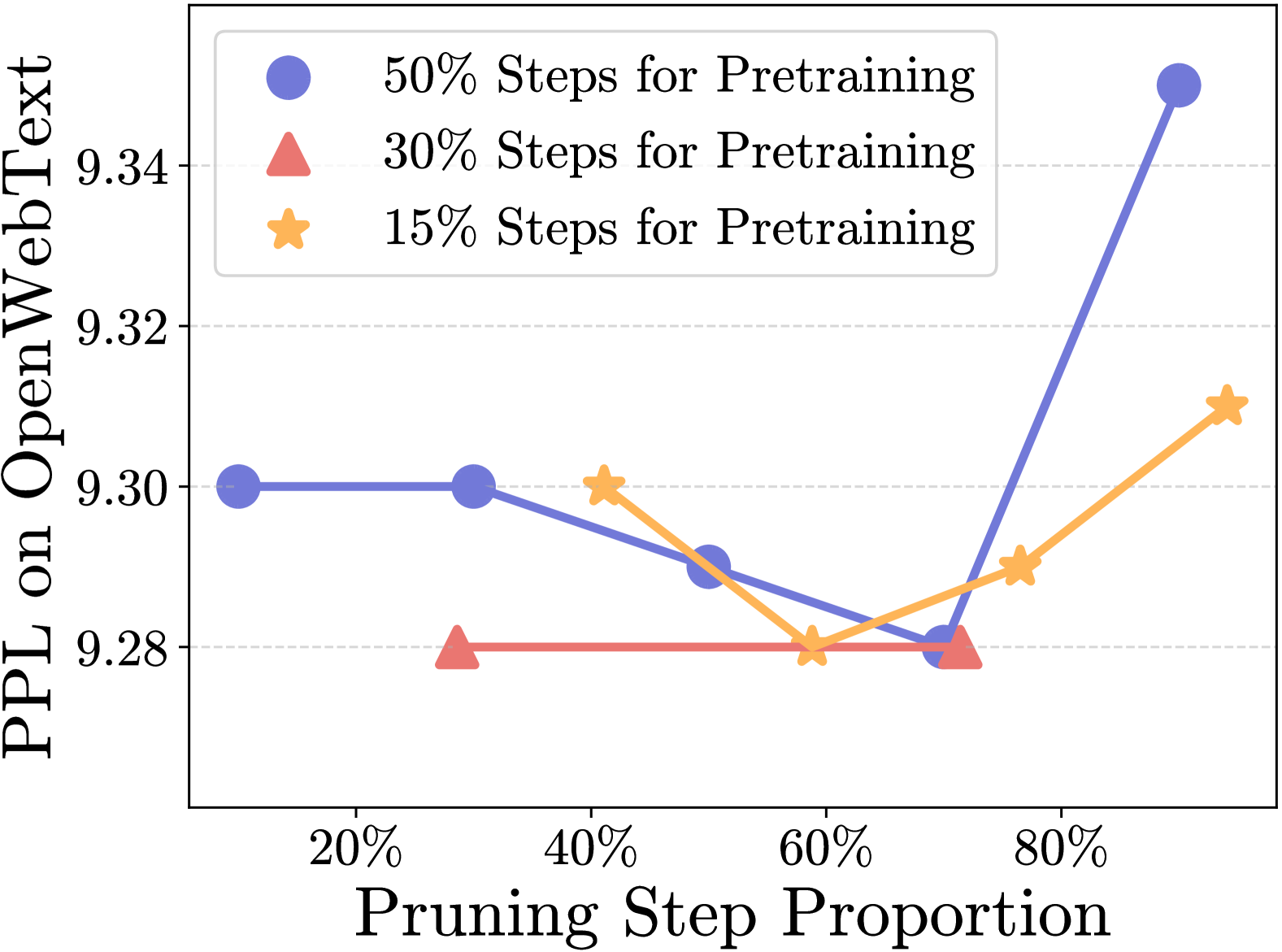
(a) Pruning Schedule

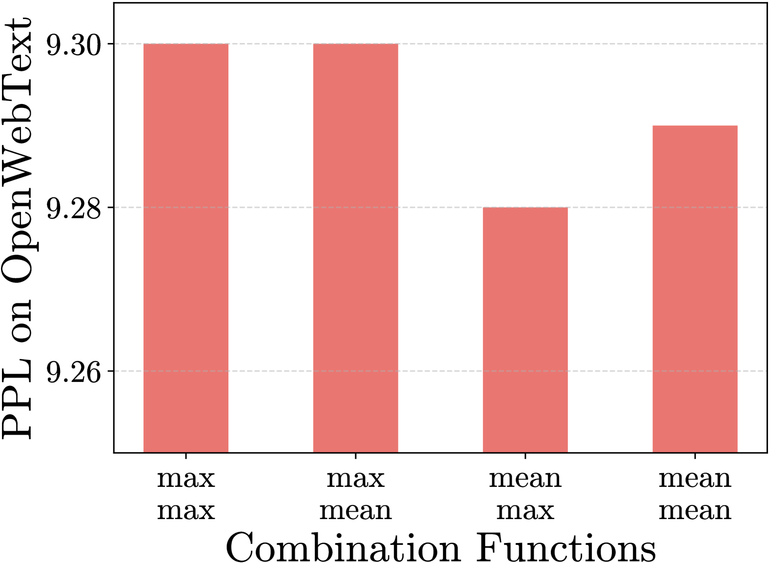
(b) Importance Combination

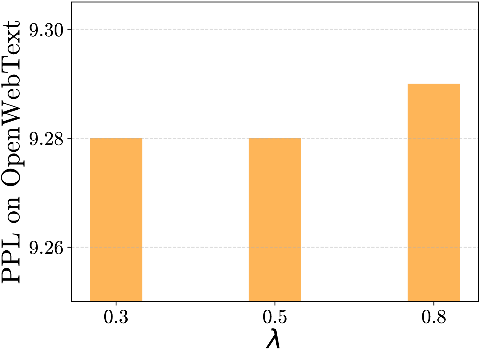
(c) EMA Coefficient $\lambda$

Figure 4: Hyperparameter study. Figure 4(a) shows the a wide range of pipeline schedule works for the best performance. Figure 4(b) implies ”mean-max” is the best choice of $f_{1}$ and $f_{2}$, though the others do not show significant degradation. Figure 4(c) shows the exponential moving average coefficient $\lambda$ is robust in a wide range from 0.3 to 0.8.

Importance Score Combination. We study how the choice of importance score combination function $f_{1}(\cdot)$ and $f_{2}(\cdot)$ in (3.2) affects the model performance. We try $\max(\cdot)$ and ${\rm mean}(\cdot)$ for each of $f_{1}(\cdot)$ and $f_{2}(\cdot)$. As shown in Figure 4(b), ”mean-max” is the best choice of $f_{1}$ and $f_{2}$, though the others do not show significant degradation.

Moving Average Coefficient. We investigate the impact of the coefficient $\lambda$ in (3.1), exploring values of 0.3, 0.5, and 0.8. A lower coefficient tends to favor current-step importance scores. Figure 4(c) indicates the optimal $\lambda$ lies between 0.3 and 0.5, with 0.8 also acceptable.

5.4 Extension of Integrated Pipeline

We demonstrate that our integrated pipelines are extensible beyond the proposed iterative structured pruning method. For OSRP and Minitron, we apply one-shot pruning to the intermediate checkpoint (2.8B-2T@1T). For Sheared LLaMA, we perform mask learning initialized from the same checkpoint using two distinct learning rate schedules: a resumed schedule for weight matrices and a fully decaying schedule for auxiliary parameters. We conduct recovery training for the pruned models using the resumed learning rate schedule described in Section 5.1.

As shown in Table 3, the integrated enlarge-and-prune pipeline shows improvement over the naive enlarge-and-prune pipeline across all pruning methods. The improvement on MMLU is the most significant, which implies the rising learning rate in naive enlarge-and-prune pipelines causes the knowledge loss the most.

Table 3: Extension of the the integrated enlarge-and-prune pipeline with OSPR, Minitron, and Sheared LLaMA pruning methods. We prune a 2.8B model to 1.3B with 2T tokens. We report the perplexity on OpenWebText, the average accuracy on comprehensive tasks, and 5-shot accuracy on MMLU. The best results are in bold.

Method	Pipeline	OpenWebText$\downarrow$	Comp Avg $\uparrow$	MMLU $\uparrow$
OSRP	Naive	8.98	40.6	32.5
	Integrated	8.93	41.7	42.9
Minitron	Naive	8.97	41.0	31.4
	Integrated	8.92	41.4	43.9
Sheared LLaMA	Naive	8.96	41.0	33.4
	Integrated	8.89	42.6	42.4

6 Combination of Knowledge Distillation

Knowledge distillation (KD) (Kim & Rush, 2016; Hinton, 2015) is another prominent approach for developing models with the help of enlarged models, wherein a small student model learns to mimic a large teacher model. Recent research (Team et al., 2024; Liang et al., 2023; Gunter et al., 2024; Li et al., 2023) finds pruning and distillation are complementary to each other and often applies them together to obtain high performance models from existing pretrained models. As we have stated in Section 1, we are interested in the token efficiency of the entire process, including the teacher model training in KD. Therefore, we study how distillation affects the enlarge-and-prune pipeline given fixed training tokens for the enlarged (teacher) model pretraining, pruning, and pruned model recovery.

To start with, we train a 2.8B-2T model using 2T tokens as the teacher model. We establish a KD baseline by training a 1.3B model from scratch over 1T tokens with KD. In our enlarge-and-prune pipeline, we prune and train the 2.8B-2T@1T intermediate checkpoint using a resumed cosine learning rate schedule for 1T tokens—equivalent to the integrated pipeline with 2T tokens as shown in Section 5.1. During pruning and recovery, we use the 2.8B-2T model as the KD teacher.

As shown in Table 4, pruning with distillation outperforms the pruning baseline across most benchmarks and surpasses the KD baseline on all benchmarks, particularly on OpenWebText and MMLU. These results reinforce our earlier conclusion in Section 4.2 and extend it to KD regime: carefully conducted enlarge-and-prune pipelines, e.g., IDEA Prune, can exceed the performance of target-size models trained from scratch using KD.

Table 4: Enlarge-and-prune pipeline with KD. Teacher model size: 2.8B-2T. The KD baseline: training a 1.3B model for 1T tokens with KD from scratch. pruning w/ KD: pruning (including recovery) the 2.8B-2T@1T checkpoint for 1T tokens with KD.

Method	OpenWebText	Arc-C	Hellaswag	TriviaQA	MMLU
Pruning w/o KD	8.879	39.0	54.0	31.1	46.4
1.3B-1T w/ KD	8.949	39.6	52.2	31.7	44.5
Pruning w/ KD	8.862	39.8	52.7	32.0	46.6

7 Conclusion

We examine token efficiency of pruning through enlarge-and-prune pipelines and propose IDEA Prune, an integrated approach that combines enlarged model pretraining, pruning, and recovery under a single cosine learning rate schedule. Through experiments compressing 2.8B models to 1.3B with 2T tokens, IDEA Prune demonstrates significant improvements over naive pipelines. Notably, we find that intermediate checkpoints provide better pruning initialization than fully converged ones under IDEA Prune, and that our approach complements knowledge distillation techniques. These insights establish a more efficient paradigm for model compression in generative language model pretraining.

Appendix A Adam Optimization

Adam optimization algorithm is popular in training large language models. Given a weight matrix $\bm{W}^{(t-1)}$ at the $t$-th step, we update the matrix $\bm{W}^{(t-1)}$ from the last step by

$$\bm{W}^{(t)}=\bm{W}^{(t-1)}-\gamma^{(t)}\widetilde{\bm{G}}^{(t)},$$

where $\gamma^{(t)}$ is the learning rate, which is often scheduled by a cosine annealing with a linear warm-up, and $\widetilde{\bm{G}}^{(t)}$ is calculated as

$$\widetilde{\bm{G}}^{(t)}=\frac{\widetilde{\bm{M}}^{(t)}}{\sqrt{\widetilde{\bm{V}}^{(t)}}+\epsilon},$$

where $\epsilon$ is a hyperparameter, and $\widetilde{\bm{M}}^{(t)},\widetilde{\bm{V}}^{(t)}$ is determined by $\bm{G}^{(t-1)}$, the gradient of $\bm{W}^{(t-1)}$, and the optimization states $\bm{M}^{(t-1)},\bm{V}^{(t-1)}$. Specifically, we update the $\bm{M}^{(t-1)},\bm{V}^{(t-1)}$ by

$$\bm{M}^{(t)} =\beta_{1}\bm{M}^{(t-1)}+(1-\beta_{1})\bm{G}^{(t-1)},$$

$$\bm{V}^{(t)} =\beta_{2}\bm{V}^{(t-1)}+(1-\beta_{2})\bm{G}^{(t-1)}\odot\bm{G}^{(t-1)},$$

where $\beta_{1}$ and $\beta_{2}$ are hyperparameters. Then, $\widetilde{\bm{M}}^{(t)}$ and $\widetilde{\bm{V}}^{(t)}$ are calculated as

$$\widetilde{\bm{M}}^{(t)} =\bm{M}^{(t)}/(1-\beta_{1}^{t}),$$

$$\widetilde{\bm{V}}^{(t)} =\bm{V}^{(t)}/(1-\beta_{2}^{t}).$$

Appendix B Cubical Sparsity Schedule in Iterative Pruning

The sparsity at the $t$-th step is

$$r(t;T_{p})=\begin{cases}0&0<t\leq T_{w},\\ R\left(1-\frac{t-T_{w}}{T_{p}}\right)^{3}&T_{w}<t\leq T_{w}+T_{p},\\ R&T_{w}+T_{p}<t\leq T,\end{cases}$$

where $R$ is the target sparsity, and $T_{w},T_{p},T$ are the number of pruning warmup steps, iterative pruning steps, total iterative pruning steps, respectively. Note that we set $T_{w}=0$ if the iterative pruning is in integrated enlarge-and-prune pipelines, and it is set to the same as the learning rate warmup steps if it is in naive enlarge-and-prune pipelines.

Appendix C Activation-based Pruning

We denote the activation of the $n$-th data sample of an FFN layer as

$$\bm{Z}^{(n)}=\sigma(\bm{X}^{(n)}\bm{W}_{\rm up}^{\top})\odot(\bm{X}^{(n)}\bm{W}_{\rm gate}^{\top}),$$

where $\bm{Z}^{(n)}\in\mathbb{R}^{l\times h}$, $l$ is the sequence length. The importance score of the $i$-th neuron is defined as

$$\bm{c}_{i}=\frac{1}{B}\sum_{n=1}^{B}\|\bm{Z}_{[:,i]}^{(n)}\|_{2},$$

where $B$ is the size of the calibration dataset (a random subset of the pre-training corpus), $\bm{z}_{[:,i]}^{(n)}$ is the $i$-th column of $\bm{Z}^{(n)}$, and $||\cdot||_{2}$ is the L2-norm of a vector. Following Muralidharan et al. (2024), we set $B=1024$. Finally, we apply (3.3) with $T_{p}=1$ to generate the pruning mask.

Appendix D Model Architecture

We present the key configurations of the models in Table 5.

Table 5: Model configurations. We list the key configs of the model we have used in this paper.

Parameter Name	1B	2.8B	300M
input length	4096	4096	4096
input dimension	2048	2048	1024
# attention heads	32	32	16
hidden dimension	6528	16384	3072
# layers	24	24	24

Appendix E Full Table

We present the full tables that are compressed in Section 5.1 and Section 5.4 due to the paper length limit. The full version of Table 2 is Table 6. The full version of Table 3 is Table 7.

Table 6: Ablation of the initialization and the learning rate schedule in enlarge-and-prune pipelines. No Train: the enlarged model without any further pruning or training. Our integrated enlarge-and-prune pipeline is equivalent to 2.8B-2T@1T initialization with a resumed learning rate schedule. Target size: 1.3B.

Model	LR Schedule	OpenWebText$\downarrow$	Arc-C$\uparrow$	Hellaswag$\uparrow$	TriviaQA$\uparrow$	MMLU$\uparrow$
2.8B-2T@1T	-	9.99	38.7	51.6	24.8	26.0
1.3B pruned from 2.8B-2T@1T	Resumed	8.88	39.0	54.0	31.1	46.4
	Restarted	8.94	39.7	54.5	30.1	37.0
2.8B-2T@1T	-	8.12	44.5	56.9	37.3	50.8
1.3B pruned from 2.8B-1T@1T	Resumed	8.89	39.3	53.6	31.8	38.2
	Restarted	8.95	39.9	53.3	31.0	36.8

Table 7: Extension of the the integrated enlarge-and-prune pipeline with OSPR, Minitron, and Sheared LLaMA pruning methods. We prune a 2.8B model to 1.3B with 2T tokens. We report the perplexity on OpenWebText, the average accuracy on comprehensive tasks, and 5-shot accuracy on MMLU.

Method		OpenWebText$\downarrow$	Arc-C$\uparrow$	Hellaswag$\uparrow$	TriviaQA$\uparrow$	MMLU$\uparrow$
OTRP	Naive	8.980	38.9	53.4	29.6	32.5
	Unified	8.926	41.1	53.8	30.1	42.9
Minitron	Naive	8.973	38.7	53.6	30.7	31.4
	Unified	8.916	39.8	53.6	30.8	43.9
Sheared LLaMA	Naive	8.960	39.4	53.6	30.1	33.4
	Unified	8.892	43.2	54.0	30.5	42.4

References

- Abdin et al. (2024) Abdin, M., Jacobs, S. A., Awan, A. A., Aneja, J., Awadallah, A., Awadalla, H., Bach, N., Bahree, A., Bakhtiari, A., Behl, H., et al. Phi-3 technical report: A highly capable language model locally on your phone. arXiv preprint arXiv:2404.14219, 2024.
- Clark et al. (2018) Clark, P., Cowhey, I., Etzioni, O., Khot, T., Sabharwal, A., Schoenick, C., and Tafjord, O. Think you have solved question answering? try arc, the ai2 reasoning challenge. arXiv:1803.05457v1, 2018.
- Ding et al. (2019) Ding, X., Zhou, X., Guo, Y., Han, J., Liu, J., et al. Global sparse momentum sgd for pruning very deep neural networks. Advances in Neural Information Processing Systems, 32, 2019.
- Dubey et al. (2024) Dubey, A., Jauhri, A., Pandey, A., Kadian, A., Al-Dahle, A., Letman, A., Mathur, A., Schelten, A., Yang, A., Fan, A., et al. The llama 3 herd of models. arXiv preprint arXiv:2407.21783, 2024.
- Gokaslan et al. (2019) Gokaslan, A., Cohen, V., Pavlick, E., and Tellex, S. Openwebtext corpus. http://Skylion007.github.io/OpenWebTextCorpus, 2019.
- Gunter et al. (2024) Gunter, T., Wang, Z., Wang, C., Pang, R., Narayanan, A., Zhang, A., Zhang, B., Chen, C., Chiu, C.-C., Qiu, D., et al. Apple intelligence foundation language models. arXiv preprint arXiv:2407.21075, 2024.
- Hendrycks et al. (2020) Hendrycks, D., Burns, C., Basart, S., Zou, A., Mazeika, M., Song, D., and Steinhardt, J. Measuring massive multitask language understanding. arXiv preprint arXiv:2009.03300, 2020.
- Hinton (2015) Hinton, G. Distilling the knowledge in a neural network. arXiv preprint arXiv:1503.02531, 2015.
- Hoffmann et al. (2022) Hoffmann, J., Borgeaud, S., Mensch, A., Buchatskaya, E., Cai, T., Rutherford, E., Casas, D. d. L., Hendricks, L. A., Welbl, J., Clark, A., et al. Training compute-optimal large language models. arXiv preprint arXiv:2203.15556, 2022.
- Jiang et al. (2023) Jiang, A. Q., Sablayrolles, A., Mensch, A., Bamford, C., Chaplot, D. S., Casas, D. d. l., Bressand, F., Lengyel, G., Lample, G., Saulnier, L., et al. Mistral 7b. arXiv preprint arXiv:2310.06825, 2023.
- Jiang et al. (2024) Jiang, A. Q., Sablayrolles, A., Roux, A., Mensch, A., Savary, B., Bamford, C., Chaplot, D. S., Casas, D. d. l., Hanna, E. B., Bressand, F., et al. Mixtral of experts. arXiv preprint arXiv:2401.04088, 2024.
- Joshi et al. (2017) Joshi, M., Choi, E., Weld, D. S., and Zettlemoyer, L. Triviaqa: A large scale distantly supervised challenge dataset for reading comprehension. arXiv preprint arXiv:1705.03551, 2017.
- Kaplan et al. (2020) Kaplan, J., McCandlish, S., Henighan, T., Brown, T. B., Chess, B., Child, R., Gray, S., Radford, A., Wu, J., and Amodei, D. Scaling laws for neural language models. arXiv preprint arXiv:2001.08361, 2020.
- Kim & Rush (2016) Kim, Y. and Rush, A. M. Sequence-level knowledge distillation. arXiv preprint arXiv:1606.07947, 2016.
- Kwon et al. (2022) Kwon, W., Kim, S., Mahoney, M. W., Hassoun, J., Keutzer, K., and Gholami, A. A fast post-training pruning framework for transformers. Advances in Neural Information Processing Systems, 35:24101–24116, 2022.
- Li et al. (2024) Li, J., Fang, A., Smyrnis, G., Ivgi, M., Jordan, M., Gadre, S., Bansal, H., Guha, E., Keh, S., Arora, K., et al. Datacomp-lm: In search of the next generation of training sets for language models. arXiv preprint arXiv:2406.11794, 2024.
- Li et al. (2023) Li, Y., Yu, Y., Zhang, Q., Liang, C., He, P., Chen, W., and Zhao, T. Losparse: Structured compression of large language models based on low-rank and sparse approximation. In International Conference on Machine Learning, pp. 20336–20350. PMLR, 2023.
- Li et al. (2020) Li, Z., Wallace, E., Shen, S., Lin, K., Keutzer, K., Klein, D., and Gonzalez, J. Train big, then compress: Rethinking model size for efficient training and inference of transformers. In International Conference on machine learning, pp. 5958–5968. PMLR, 2020.
- Liang et al. (2023) Liang, C., Jiang, H., Li, Z., Tang, X., Yin, B., and Zhao, T. Homodistil: Homotopic task-agnostic distillation of pre-trained transformers. arXiv preprint arXiv:2302.09632, 2023.
- Liu et al. (2024) Liu, A., Feng, B., Xue, B., Wang, B., Wu, B., Lu, C., Zhao, C., Deng, C., Zhang, C., Ruan, C., et al. Deepseek-v3 technical report. arXiv preprint arXiv:2412.19437, 2024.
- Liu (2019) Liu, Y. Roberta: A robustly optimized bert pretraining approach. arXiv preprint arXiv:1907.11692, 364, 2019.
- Loshchilov (2017) Loshchilov, I. Decoupled weight decay regularization. arXiv preprint arXiv:1711.05101, 2017.
- Loshchilov & Hutter (2016) Loshchilov, I. and Hutter, F. Sgdr: Stochastic gradient descent with warm restarts. arXiv preprint arXiv:1608.03983, 2016.
- Louizos et al. (2017) Louizos, C., Welling, M., and Kingma, D. P. Learning sparse neural networks through regularization. arXiv preprint arXiv:1712.01312, 2017.
- Molchanov et al. (2019) Molchanov, P., Mallya, A., Tyree, S., Frosio, I., and Kautz, J. Importance estimation for neural network pruning. In Proceedings of the IEEE/CVF conference on computer vision and pattern recognition, pp. 11264–11272, 2019.
- Muralidharan et al. (2024) Muralidharan, S., Sreenivas, S. T., Joshi, R., Chochowski, M., Patwary, M., Shoeybi, M., Catanzaro, B., Kautz, J., and Molchanov, P. Compact language models via pruning and knowledge distillation. arXiv preprint arXiv:2407.14679, 2024.
- Radford et al. (2019) Radford, A., Wu, J., Child, R., Luan, D., Amodei, D., Sutskever, I., et al. Language models are unsupervised multitask learners. OpenAI blog, 1(8):9, 2019.
- Team et al. (2024) Team, G., Georgiev, P., Lei, V. I., Burnell, R., Bai, L., Gulati, A., Tanzer, G., Vincent, D., Pan, Z., Wang, S., et al. Gemini 1.5: Unlocking multimodal understanding across millions of tokens of context. arXiv preprint arXiv:2403.05530, 2024.
- Vaswani (2017) Vaswani, A. Attention is all you need. Advances in Neural Information Processing Systems, 2017.
- Wang et al. (2019) Wang, Z., Wohlwend, J., and Lei, T. Structured pruning of large language models. arXiv preprint arXiv:1910.04732, 2019.
- Xia et al. (2022) Xia, M., Zhong, Z., and Chen, D. Structured pruning learns compact and accurate models. arXiv preprint arXiv:2204.00408, 2022.
- Xia et al. (2023) Xia, M., Gao, T., Zeng, Z., and Chen, D. Sheared llama: Accelerating language model pre-training via structured pruning. arXiv preprint arXiv:2310.06694, 2023.
- Zellers et al. (2019) Zellers, R., Holtzman, A., Bisk, Y., Farhadi, A., and Choi, Y. Hellaswag: Can a machine really finish your sentence? arXiv preprint arXiv:1905.07830, 2019.
- Zhang et al. (2022) Zhang, Q., Zuo, S., Liang, C., Bukharin, A., He, P., Chen, W., and Zhao, T. Platon: Pruning large transformer models with upper confidence bound of weight importance. In International conference on machine learning, pp. 26809–26823. PMLR, 2022.
- Zhu & Gupta (2017) Zhu, M. and Gupta, S. To prune, or not to prune: exploring the efficacy of pruning for model compression. arXiv preprint arXiv:1710.01878, 2017.