Reassessing the boundary between classical and nonclassical
for individual quantum processes

Abstract

There is a received wisdom about where to draw the boundary between classical and nonclassical for various types of quantum processes. For instance, for multipartite states, it is the divide between separable and entangled, for channels, the divide between entanglement-breaking and not, for sets of measurements, the divide between compatible and incompatible, and for assemblages, the divide between steerable and unsteerable. However, no unified justification of these placements of the classical-nonclassical divide has been proposed. That is, although each might be motivated by some notion of what it means to be classically explainable, it is not the same notion for all of them. One well-motivated notion of classical explainability is the one based on generalized noncontextuality: a set of circuits is classically explainable if the statistics they generate can be realized by a generalized-noncontextual ontological model. In this work, we show that this notion can be leveraged to define a classical-nonclassical divide for individual quantum processes of arbitrary type. A set of measurements, for example, is judged to be classical if and only if a particular set of circuits—the one obtained by contracting these measurements with every possible quantum state—is classically explainable in the sense just articulated. We begin the task of characterizing where the classical-nonclassical divide lies according to this proposal for a variety of different types of processes. In particular, we show that all of the following are judged to be nonclassical: every entangled state, every set of incompatible measurements, every non-entanglement-breaking channel, every steerable assemblage. Our proposal differs from the received wisdom, however, insofar as it also judges certain subsets of the complementary classes to be nonclassical, i.e., certain separable states, compatible sets of measurements, entanglement-breaking channels, and unsteerable assemblages. We also prove a structure theorem characterizing the classical-nonclassical divide in terms of whether or not a preparation or measurement process has a certain type of frame representation.

I Introduction

A recurring question of interest in quantum information and foundations is to determine which processes (states, measurements, sets of measurements, channels, and so on) can be reasonably said to be classical, and which must be acknowledged to be nonclassical (that is, genuinely quantum).

In much of the literature, proposals for the placement of the classical-nonclassical divide have been introduced on a case-by-case basis for different types of processes. For instance, it is commonly assumed that for bipartite states, it is the divide between separable and entangled, for channels, it is the divide between entanglement-breaking and non-entanglement-breaking, for multi-measurements, the divide between the set of measurements being compatible and being incompatible, and so on.

These proposals are often based on intuitive notions of what should count as a classical kind of correlation or process. The question of whether all such proposals are consistent with a single principle, however, has remained largely unexplored. Indeed, the resulting conceptions of nonclassicality can be distinct for different types of processes, and we will even show that they are sometimes in conflict with one another.

Seeking to define classicality for different types of processes using a unified notion of classical explainability is especially important given that many widely held intuitions about what features of quantum theory are evidence of genuine quantumness have turned out not to be consistent with well-motivated notions of classical explainability. For example, there exist classical theories [4, 5, 6] that satisfy various principles, such as locality and generalized noncontextuality, and that nonetheless contain analogues of entanglement, non-entanglement-breaking channels, and incompatible measurements, not to mention steering, interference, no-cloning, and a wide variety of other phenomena that are commonly thought to be difficult to explain classically.

The question of where the classical-nonclassical divide lies is sometimes mistaken for one that is merely about semantics, that is, merely about how we use the term “classical”. This is not the case because the answer to this question has a significant impact on how one pursues foundational and applied research in quantum theory. For instance, the answer impacts how one pursues the project of identifying quantum-over-classical advantages for various tasks (computational, cryptographic, metrological, thermodynamic, etcetera) because one only expects to find such advantages in protocols that leverage nonclassical resources. In other words, a desideratum for a good proposal on where to place the classical-nonclassical divide is that any advantage should require resources that are deemed nonclassical by the proposal. Similarly, the placement of the classical-nonclassical divide is important for identifying the manner in which the quantum worldview differs from the classical worldview and hence for correctly identifying the true innovation of quantum theory over its classical predecessors.

Here, we introduce an approach that defines the classical-nonclassical divide for a process based on a single principle, namely the idea that classical explainability of operational statistics corresponds to realizability by a generalized-noncontextual ontological model  [7, 8].

Since our framework is based on the notion of a generalized-noncontextual ontological model, it is worth reiterating the motivations for why realizability in such a model constitutes a good notion of classical explainability of operational statistics. First, the ontological models framework captures the conventional, hence classical, ways of understanding causation and inference [9]. Second, the principle of generalized noncontextuality is an instance of a methodological principle for theory-construction due to Leibniz that has proven its utility in physics through Einstein’s use of it in his development of the special and general theories of relativity [10]. A generalized-noncontextual ontological representation is also equivalent to a positive quasiprobability representation [11, 12, 8], and coincides with the natural notion of classical explainability in the framework of generalized probabilistic theories (GPTs [13, 14]), namely, linear embeddability into the strictly classical (simplicial) GPT [12, 8].

This notion of classical explainability also has pragmatic advantages over some of its competitors. For one, it is noise-robust and is therefore testable in real experiments where the ideal of noiselessness is never realized [15]. This is in contrast to the Kochen-Specker notion of noncontextuality [16], as argued in Ref. [17].

It also has universal applicability: given a circuit with arbitrary causal structure, one can ask whether or not there exists a generalized-noncontextual ontological model that can reproduce the statistics generated by that circuit. In contrast, Bell inequalities [18] apply only to circuits having one specific causal structure. Due to its universal applicability, one can ask: for any operational phenomenon, precisely which aspects of it fail to admit of a generalized-noncontextual ontological model and hence which aspects resist classical explanation? Results establishing facts about the boundary between what is classically explainable and what is not are now known for the phenomenology of: quantum computation [19, 20], state discrimination [21, 22, 23, 24], interference [6, 25, 26, 27], compatibility [28, 29, 30], uncertainty relations [31], metrology [32], thermodynamics [32, 33, 34], weak values [35, 36], coherence [37, 38, 39], quantum Darwinism [40], information processing and communication [41, 42, 43, 44, 45, 46, 47], cloning [48], broadcasting [49], pre- and post-selection paradoxes [50], randomness certification [51], psi-epistemicity [52], macroscopic realism [53], and Bell [54, 9] and Kochen-Specker scenarios [55, 56, 57, 58, 59, 60, 61]. Aiding this research is a growing set of powerful techniques for certifying the failure to admit of a noncontextual ontological model [62, 63, 64, 8, 12, 65, 66, 67, 68, 15, 69].

However, in all work to date, the existence of a generalized-noncontextual ontological model provides a notion of classical explainability for a closed circuit, since only such a circuit can generate operational statistics and it is on the basis of these statistics that classical explainability is assessed. In contrast, no notion of classicality has been given for a single process within a circuit, such as a single quantum state, a single quantum measurement, or a single quantum channel. In this work, we propose a way of doing so.

The intuitive idea is straightforward: a given quantum process is nonclassical if and only if there exists a quantum circuit that leverages it nontrivially to generate statistics that are inconsistent with a generalized-noncontextual ontological model. In Section III, we formalize this definition. In particular, we explain what it means to “leverage in a nontrivial way” the process, and then we simplify the definition considerably, by showing that rather than considering all quantum circuits containing the process, one need only consider circuits where product states are prepared on its inputs and product measurements are implemented on its outputs.

We then undertake the task of characterizing which quantum preparations, measurements, and transformations are nonclassical, and which are classical. (This paper focuses only on quantum theory, although our approach could be applied to an arbitrary generalized probabilistic theory.) For instance, we prove the following results:

1. A single state on a unipartite system is always classical.

2. Any set of distinct pure states on a unipartite system is nonclassical if and only if the states are linearly dependent in the operator space (and therefore any tomographically complete set of pure states is classical).

3. Any rank-1 POVM is nonclassical if and only if its POVM elements are linearly dependent in the operator space. (and therefore any symmetric informationally complete rank-1 POVM is classical).

4. The set of classical states (measurements) is nonconvex.

5. Every steerable assemblage is nonclassical, as are certain unsteerable assemblages.

6. Every set of incompatible measurements exhibiting incompatibility is nonclassical, as are certain sets of compatible measurements (including certain singleton sets, i.e., single measurements).

7. Every entangled state is nonclassical, as are certain separable states.

8. All non-entanglement-breaking channels are nonclassical, as are certain entanglement-breaking channels.

In addition, we prove several more general results. We prove two structure theorems characterizing which sets of states and which sets of measurements are classical. We then prove that a single bipartite state is nonclassical if there is some set of measurements (on either subsystem) that steers the other system to a nonclassical set of states. We generalize this result to multipartite states, and we then reduce the problem of deciding nonclassicality of a quantum process of any type (including channels, instruments, and so on) to the problem of deciding nonclassicality of a corresponding multipartite state. Together, these results provide a useful characterization of the nonclassicality of arbitrary processes.

In a companion paper [70], we provide further tools based on semidefinite programming that help one to witness and quantify the nonclassicality of single states and measurements. We do so both in a theory-dependent way (analogous to entanglement witnesses) and in a theory-independent way (using noncontextuality inequalities).

Finally, we wish to head off a possible point of confusion: the term “quantum” is sometimes taken as a synonym for nonclassical, and other times taken as an enveloping term that includes classical and nonclassical as special cases.  In this work, we use the term “quantum” in the more inclusive sense. This is because we are studying the question of which subsets of phenomena described by quantum theory are classically explainable and which are not. We use the term “nonclassical” or “intrinsically quantum” to signal the impossibility of classical explanation. 

II Preliminaries

II.1 Types of quantum processes

A generic process in quantum theory is simply a channel with various input and output systems, which may be quantum or classical. A classical system that is an input is generally called a setting variable and one that is an output is generally called an outcome variable. The most common examples of processes in quantum theory are states, effects, measurements, channels, and instruments. However, it is often useful to consider more general processes, including those listed in the Table 1.

Process Type	Quantum Rep’n	Ontological Rep’n
State	$\rho$	$p(\lambda|\rho)$
Effect	$M$	$p(M|\lambda)$
Channel	$\mathcal{E}$	$p(\lambda^{\prime}|\lambda)$
Measurement	$\{M_{b}\}_{b}$	$\{p(b|\lambda)\}_{b}$
Instrument	$\{\mathcal{F}_{c}\}_{c}$	$\{p(c\lambda^{\prime}|\lambda)\}_{c}$
Source	$\{p(a)\rho_{a}\}_{a}$	$\{p(a\lambda)\}_{a}$
Multi-state	$\{\rho_{\cdot|x}\}_{x}$	$\{p(\lambda|x)\}_{x}$
Multi-channel	$\{\mathcal{E}_{\cdot|z}\}_{z}$	$\{p(\lambda|z\lambda)\}_{z}$
Multi-measurement	$\{\{M_{b|y}\}_{b}\}_{y}$	$\{\{p(b|y\lambda)\}_{b}\}_{y}$
Multi-source	$\{\{p(a|x)\rho_{a|x}\}_{a}\}_{x}$	$\{\{p(a\lambda|x)\}_{a}\}_{x}$
Multi-instrument	$\{\{\mathcal{F}_{c|z}\}_{c}\}_{z}$	$\{\{p(c\lambda^{\prime}|z\lambda)\}_{c}\}_{z}$
Partial trace	$\textrm{Tr}_{A_{1}}[\rho^{A_{1}A_{2}}]$	$\sum_{\lambda_{1}}p(\lambda_{1}\lambda_{2})$

Table 1: Examples of various types of process, their representations in quantum theory, and their representations as substochastic matrices in an ontological model. Throughout this paper, we denote classical outcome variables by $a,b,c$ and setting variables by $x,y,z$.

Most of these processes will be familiar to the quantum information theorist. However, the terminology of sources, multi-sources, multi-measurements, and multi-channels is relatively new, so we explain these terms below. These processes are easily understood via a diagrammatic representation, as in Fig. 1.

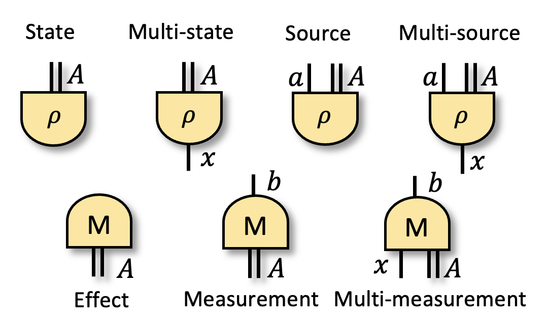
Figure 1: Examples of processes with a single quantum output $A$ (top) and with a single quantum input $A$ (bottom) on a single quantum system. Throughout this paper, quantum systems are represented by double wires, while classical systems are represented by single wires.

The type of a process is simply a specification of its input and output systems as well as a specification of whether each of these is classical or quantum. Diagrammatically, we will depict quantum systems by double wires and classical systems by single wires (see, e.g., Fig. 1). In this approach, each individual input and output of a process (depicted by a wire in the diagram) is considered a fundamental system, having no subsystem structure, so that a composite system is always described by a collection of inputs or a collection of outputs.

Each quantum input and output for a given process is associated with a Hilbert space. For a quantum system $A$, we denote this Hilbert space by $\mathcal{H}^{A}$. We will denote the set of all linear operator on $\mathcal{H}$ as $\mathcal{L}(\mathcal{H})$, the set of all Hermitian operators on $\mathcal{H}$ as $\text{Herm}(\mathcal{H})$, the set of all density operators (i.e., all $\rho\in\text{Herm}(\mathcal{H})$ such that $\rho\geq 0$ and $\textrm{Tr}[\rho]=1$) as $\mathcal{S}(\mathcal{H})$, and the set of all effects (i.e., all $M\in\text{Herm}(\mathcal{H})$ such that $0\leq M\leq\mathbb{1}$) as $\mathcal{M}(\mathcal{H})$.

It is useful to classify the types of processes by their quantum inputs and outputs, such that the only differences among the processes in a given class is in their classical inputs and outputs. For instance, processes with a single quantum output and no quantum input form a class. We will refer to these as processes of the preparation variety. In a similiar fashion, the class of processes with a single quantum input and no quantum output will be termed processes of the measurement variety and the class of processes with both a quantum input and a quantum output will be termed processes of the transformation variety. We will sometimes qualify the terms describing these varieties to stipulate the subsystem structure of the quantum inputs or the quantum outputs; for example, we will speak of processes of the bipartite preparation variety.

We begin with processes of the preparation variety having a single quantum output $A$. Four types of processes in this class are depicted in the top row of Fig. 1. A single deterministic preparation on a quantum system $A$ is represented by a density operator (or state) $\rho\in\mathcal{S}(\mathcal{H}^{A})$. A process with a classical input $x$ (a setting variable) that determines which of a set of preparations is implemented on $A$ can be represented by a set of states $\{\rho_{\cdot|x}\}_{x}$. We call such a process a multi-state. Next, consider a process in which a variable $a$ is sampled at random from a distribution $p(a)$ and then the preparation represented by the state $\rho_{a}$ is implemented on $A$ and the variable $a$ becomes a classical output of the process (an outcome variable) that flags which state was prepared. Such a process is represented by a set of unnormalized states $\{p({a})\rho_{a}\}_{a}$, and we refer to it as a source (it is sometimes termed an ensemble). Finally, a process with a classical input $x$ (a setting variable) that determines which of a set of sources is implemented can be represented by a set of sets of unnormalized states $\{\{p(a|x)\rho_{a|x}\}_{a}\}_{x}$. We refer to such a process as a multi-source (such processes arise in steering scenarios, where they are termed assemblages). We will sometimes write $\mathsf{P}\coloneqq\{\mathsf{P}_{x}\}_{x}\coloneqq\{\{p(a|x)\rho_{a|x}\}_{a}\}_{x}$.

Next, we turn to processes of the measurement variety, having a single quantum input $A$. Three types of processes in this class are depicted in the bottom row of Fig. 1. (Note that the term measurement is used here to refer specifically to processes with no quantum output, such that there is only a retrodictive aspect to be characterized. Processes with a classical outcome that have both a quantum input and a quantum output will here be termed instruments and are discussed below.) In quantum theory, a measurement with outcome labelled by $b$ is represented by a positive-operator valued measure (POVM) $\{M_{b}\}_{b}$ where each $M_{b}\in\mathcal{M}(\mathcal{H}^{A})$. The process that describes implementing this measurement and obtaining the outcome $b$ (so that it can be represented as a process with no classical outcome) is termed an effect and is represented by the single operator $M_{b}\in\mathcal{M}(\mathcal{H}^{A})$. We use the term multi-measurement to refer to a process with a classical input $y$ (a setting variable) that determines which of a set of measurements is implemented. It can be represented by a set of POVMs, $\mathsf{M}\coloneqq\{\mathsf{M}_{y}\}_{y}\coloneqq\{\{M_{b|y}\}_{b}\}_{y}$. Note that the notion of a measurement is subsumed as a special case the notion of a multi-measurement, where the setting variable is trivial.

Finally, we consider processes of the transformation variety. A process that has a quantum input $A$ and a quantum output $B$ but that has neither a classical input nor a classical output is termed a channel and is represented by a map $\mathcal{E}:\mathcal{L}(\mathcal{H}^{A})\rightarrow\mathcal{L}(\mathcal{H}^{B})$ that is completely positive and trace-preserving [71, 72]. A process of the transformation variety that also has a classical input (a setting variable $z$) describes a set of channels $\{\mathcal{E}_{\cdot|z}\}_{z}$ and will be termed a multi-channel. A process of the transformation variety that has a classical output (an outcome variable) is termed an instrument. It can be conceived of as a measurement procedure that is nondestructive, so that the outcome is not only informative about the quantum input (the retrodictive aspect) but about the quantum output as well, and correlations between these (the transformative aspect). An instrument with outcome $c$ is represented by a set of trace-nonincreasing channels, denoted $\{\mathcal{F}_{c}\}_{c}$, that sum to a trace-preserving channel. We use the term multi-instrument to refer to a process with a classical input $z$ (a setting variable) that determines which of a set of instruments is implemented. We denote such a set of instruments by $\{\{\mathcal{F}_{c|z}\}_{c}\}_{z}$.

We will often denote the operation of sequential composition of two processes by $\circ$. For example, the application of a channel $\mathcal{E}$: $\mathcal{L}(\mathcal{H}^{A})\rightarrow\mathcal{L}(\mathcal{H}^{B})$ to a state $\rho\in\mathcal{S}(\mathcal{H}^{A})$ defines a new state $\mathcal{E}\circ\rho:=\mathcal{E}(\rho)\in\mathcal{S}(\mathcal{H}^{B})$. We will also use $\circ$ to denote more general types of “wiring together” of processes. For instance, a channel $\mathcal{E}$ from $A$ to $B$ can be slotted into a comb [73] $\mathcal{C}$ with output $A$ and input $B$ (as in Fig. 4(d) below), and we denote the resulting closed circuit by $\mathcal{C}\circ\mathcal{E}$.

Consider a quantum circuit built up from parallel and sequential composition of a set of quantum processes. Quantum theory provides a prescription for computing the operational statistics generated by any such circuit. Here and throughout this article, we use the term operational statistics (or simply statistics) to refer to the conditional probability distribution over all the outcome variables in the circuit given all the setting variables in the circuit.

Finally, we note that any classical inputs (setting variables) and classical outputs (outcome variables) of a process can be reconceptualized, respectively, as quantum inputs and quantum outputs that are dephased in a particular basis. For example, a multi-measurement can be viewed as a channel that has two quantum inputs, one of which is dephased (this one corresponds to the setting variable) and that has a single dephased quantum output (which corresponds to the outcome variable). As we will show in Section VIII, all of our results are invariant under this reconceptualization of the type of a process.

II.2 Classical explainability of the statistics generated by a set of quantum circuits

As noted in the introduction, we take classical explainability of operational statistics to mean the possibility of reproducing these operational statistics in a generalized-noncontextual ontological model.

We here wish to conceptualize quantum theory as an operational theory wherein one has quotiented the set of laboratory procedures of a given type with respect to an operational equivalence relation [74]. (This is the standard conceptualization in the field of quantum information, where a state is a density operator, a channel is a completely-positive trace-preserving map, and a measurement outcome is a POVM element.) We digress briefly to explain this. In an unquotiented operational theory, a given procedure (preparation, measurement, transformation, etc.) is conceptualized as a list of laboratory instructions [75], so that the theoretical description includes details that can be irrelevant to the operational statistics obtained in circuits within which the procedure is embedded. Despite their irrelevance to the operational statistics, such details—which are termed contexts—might still be relevant to the ontological representation of the procedure in a contextual ontological model [75]. Sameness of operational statistics defines an equivalence relation over procedures. A quotiented operational theory is one that only includes operational equivalence classes of procedures, and does not include the details (i.e., contexts) that distinguish the procedures within a given class. For example, an equivalence class of preparation procedures in quantum theory corresponds to a density operator.

Conceptualizing quantum theory as a quotiented operational theory introduces a subtlety regarding how to understand the notion of classical explainability, namely, that the definition of a generalized-noncontextual ontological model was originally given only for unquotiented operational theories. Because a quotiented operational theory has quotiented away the notion of context that would be leveraged in a context-dependent ontological representation, one cannot define classical explainability of such a theory as the possibility of reproducing its operational statistics in terms of a generalized-noncontextual ontological model.

What is required is a translation of the notion of classical explainability described above into the language of quotiented operational theories. Such a translation was presented in Ref. [12, 8]. It is this: a quotiented operational theory is classically explainable if and only if its predictions can be reproduced by an ontological theory that is obtained from the quotiented operational theory by a linear and diagram-preserving ontological representation map, where each operational process is mapped to a substochastic map.

Consequently, this is our notion of classical explainability:

Definition 1.

The statistics generated by a set of quantum circuits of a given structure are classically explainable if and only if they admit of a linear and diagram-preserving ontological representation—that is, if and only if there is a linear and diagram-preserving map from the quantum systems appearing in the circuit to random variables, and from the quantum processes appearing in the set of circuits to substochastic matrices [8] that preserves the statistical predictions [8].

Note that we will sometimes simply say that the set of circuits itself (rather than its statistics) is classically explainable. Note also that we will often consider situations where the set of circuits in question contains only one element, in which case we will speak of the classical explainability of a circuit rather than of a set of circuits (an example of this follows). This notion of classical explainability of a set of circuits is equivalent to the notion defined by the possibility of a generalized-noncontextual ontological model of an unquotiented version of the set of circuits [8], the motivations for which were discussed in the introduction.

This definition relies on an abstract notion of a linear and diagram-preserving (or functorial [76]) map from quantum processes in the circuit(s) to substochastic matrices over random variables. The advantage of this definition is that it is simple to state, simple to visualize (see Figure 2), and fully general, in the sense that it applies to arbitrary circuits. The disadvantage is that to write it down more formally and explicitly requires a diagrammatic formalism like that presented in Ref. [8]. As many readers may not be familiar with this diagrammatic notation, we will not repeat the general definitions here, but will instead only give the explicit form for specific examples (for which standard algebraic notations suffice).

As a first illustrative example, imagine one implements an experiment with circuit of the sort shown in Figure 2, with multi-state $\{\rho_{\cdot|x}\}_{x}$, multi-channel $\{\mathcal{E}_{\cdot|z}\}_{z}$, and measurement $\{M_{b}\}_{b}$. This circuit belongs to a more general scenario, which is typically referred to as a prepare-transform-measure scenario. (Ref. [64] begins the systematic study of such scenarios using noncontextuality inequalities.)

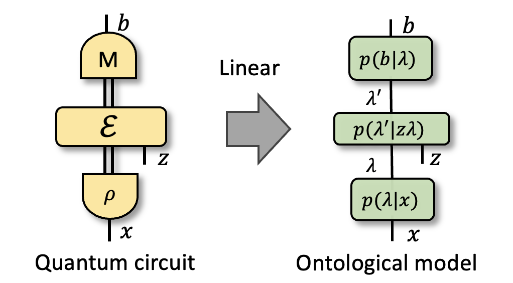
Figure 2: A prepare-transform-measure circuit (left) and an ontological representation of it (right). The circuit is classically explainable if and only if there exists a linear and diagram-preserving ontological representation taking each quantum system to a classical random variable and each quantum process to a substochastic matrix. The map must moreover respect the circuit’s topology and reproduce the quantum predictions.

The operational (quantum) statistics one can generate within such a circuit are

$$p(b|xz)={\rm Tr}[M_{b}\mathcal{E}_{\cdot|z}(\rho_{\cdot|x})].$$ (1)

A linear and diagram-preserving ontological representation for such a circuit provides a realist explanation of these statistics in terms of some underlying space of ontic states that encapsulate the fundamental properties of the system in question and that ultimately determine the outcomes of measurements on the system. In particular, it associates with each system $S$ in the circuit an ontic state space $\Lambda_{S}$ stipulating the set of all possible ontic states. (We assume this set is finite for simplicity of the presentation.) Each state $\rho_{\cdot|x}$ is associated with a probability distribution over $\Lambda$, namely $p(\lambda|x)$, where $p(\lambda|x)\geq 0$ and $\sum_{\lambda}p(\lambda|x)=1.$ Each channel $\mathcal{E}_{\cdot|z}$ is represented by a stochastic matrix, the elements of which are conditional probabilities $p(\lambda^{\prime}|z\lambda)$ giving the probability of transitioning from ontic state $\lambda$ to $\lambda^{\prime}$; this stochastic matrix must satisfy $p(\lambda^{\prime}|z\lambda)\geq 0$ for all $\lambda,\lambda^{\prime}\in\Lambda$ and $\sum_{\lambda^{\prime}}p(\lambda^{\prime}|z\lambda)=1$ for all $\lambda\in\Lambda$. Each measurement effect $M_{b}$ is represented by a response function $p(b|\lambda^{\prime})$, describing the probability of obtaining outcome $b$ given the ontic state $\lambda^{\prime}$; each response function satisfies $1\geq p(b|\lambda^{\prime})\geq 0$, and for a set of effects $\{M_{b}\}_{b}$ summing to the identity (and so forming a valid measurement), one must have $\sum_{b}p(b|\lambda^{\prime})=1$ for all $\lambda\in\Lambda$.

Thus far, we have described the implications of the ontological representation being diagram-preserving. We now consider the additional conditions implied by the representation being linear.

First of all, there are generically constraints among the ontological representations of the states in the circuit, since the mapping from the set of states $\{\rho_{\cdot|x}\}_{x}$ to their ontological representations $\{p(\lambda|x)\}_{x}$ must be linear. So if an identity such as

$$\sum_{x}\alpha_{x}\rho_{\cdot|x}=\mathbb{0}$$ (2)

holds among the states (where here and elsewhere in the article, $\mathbb{0}$ denotes the zero operator), the corresponding identity must hold among the ontological representations of these states, namely,

$$\sum_{x}\alpha_{x}p(\lambda|x)=0,$$ (3)

for all $\lambda$. We will call constraints of the former type operational identities, and constraints of the latter type ontological identities.

Similarly, any operational identity among transformations, such as

$$\sum_{z}{\alpha}_{z}\mathcal{E}_{z}=\mathbb{0},$$ (4)

implies the corresponding ontological identity

$$\sum_{z}\alpha_{z}p(\lambda^{\prime}|z\lambda)=0$$ (5)

for all $\lambda$ and all $\lambda^{\prime}$, and any operational identity

$$\sum_{b}\alpha_{b}M_{b}=\mathbb{0}$$ (6)

among effects implies the corresponding ontological identity

$$\sum_{b}\alpha_{b}p(b|\lambda^{\prime})=0$$ (7)

for all $\lambda^{\prime}$.

Moreover, if one considers grouping together (i.e., “boxing”) the channels with either the states or effects, then the representation of these composite processes (which, by diagram preservation, is given by the composition of their representations) must also satisfy constraints from linearity. In particular, any operational identities like

$$\sum_{zx}{\alpha}_{zx}\mathcal{E}_{z}(\rho_{\cdot|x})=\mathbb{0},$$ (8a)

$$\sum_{bz}{\alpha}_{bz}\mathcal{E}_{z}^{\dagger}(M_{b})=\mathbb{0},$$ (8b)

imply the corresponding ontological identities

$$\sum_{zx}{\alpha}_{zx}\sum_{\lambda}p(\lambda^{\prime}|z\lambda)p(\lambda|x)=0,$$ (9)

$$\sum_{bz}{\alpha}_{bz}\sum_{\lambda^{\prime}}p(b|\lambda^{\prime})p(\lambda^{\prime}|z\lambda)=0,$$ (10)

for all $\lambda,\lambda^{\prime}\in\Lambda$.

Finally, the model must reproduce the empirical predictions of quantum theory, so that

$$p(b|xz)={\rm Tr}[M_{b}\mathcal{E}_{\cdot|z}(\rho_{\cdot|x})]=\sum_{\lambda\lambda^{\prime}}p(b|\lambda^{\prime})p(\lambda^{\prime}|z\lambda)p(\lambda|x).$$ (11)

These are all the constraints that hold for a linear and diagram-preserving ontological representation of the quantum circuit in Figure 2. For more general quantum circuits, the prescription is similar, but one must consider all possible ways of composing together processes within the circuit, and then demand that the operational identities on all of these effective processes are preserved in the ontological representation, in a manner analogous to what was done above. We again refer the reader to Ref. [8] for a diagrammatic framework that greatly simplifies the explicit treatment of general circuits.

It is worth emphasizing that assessments of classical explainability are always given relative to a circuit, that is, relative to a factorization of systems into subsystems and a hypothesis about the causal structure. This follows from two consequences of diagram preservation—the fact that an ontological model associates an ontic state space to each system in the given circuit, and the fact that the stochastic processes in the model must be wired together with the same connectivity as one finds in the quantum circuit. Although this choice is quite innocuous in simple cases like a prepare-measure scenario or a Bell scenario [77], it is a bit more substantive in general. We will see this in Section V when we discuss the representation of bipartite systems. The reader can also find more discussion of this point in Ref. [9, 68].

II.3 Two notions of variability in the identity of a process

There are two ways in which one can imagine variability in the identity of a process within a circuit. On the one hand, this variability might be induced by the variability in the value of a setting variable or by variability in the value of an outcome variable. This is a variability that gets explored physically in different runs of the experiment. On the other hand, we sometimes wish to contemplate a theoretical notion of variability. For instance, for a process that has neither classical inputs nor classical outputs (such as a single state or transformation), we might wish to consider all possible choices for this process according to quantum theory. We refer to the former sort of variability as realized variability and the latter as theoretical variability.

In the following, when we consider a specific quantum circuit, then for a given process within that circuit, there will be some realized variability. This type of variability is considered part of the specification of the circuit, and is captured by the range of the classical setting and outcome variables attached to that process.

However, in our assessments of classical explainability of a given type of process, we will often consider all the processes that are dual to it (in a sense to be specified). The variability in the dual process is of the theoretical variety. We are considering what quantum theory predicts for every possible choice of this dual process. For the case where the process is a state or multistate or source or multisource, the dual process is an effect. Quantum theory stipulates the probability assigned to all effects, and these probability assignments do not depend on what measurement or multi-measurement this effect is considered a part of. Similarly, for the case where the process is a measurement or a multi-measurement, the dual process is a state. Quantum theory stipulates the probability generated by all states, and these probabilities do not depend on what source or multi-source this state is considered a part of.

III Defining the classical-nonclassical divide for an individual quantum process

When should a given quantum process be deemed to be nonclassical? Intuitively, it is nonclassical if and only if (i) it can be used in some quantum circuit to realize operational statistics that are not classically explainable (in the sense of Definition 1), and (ii) it is implicated in the lack of classical explainability. We begin by clarifying what we mean by “being implicated in the lack of classical explainability”. Essentially, if a circuit realizes statistics that are not classically explainable independently of the identity of the process in question, the process is not implicated in the lack of classical explainability.

Consider the question of whether a given multi-source is nonclassical. Suppose one has the circuit in Figure 3(a), where the multi-source appears in yellow, and suppose that an ancilla system is also prepared in some state (in blue) and the composite of system and ancilla are subjected to a joint measurement. In this case, it is possible to observe nonclassicality regardless of the identity of the multi-source on the system. This can be done, for instance, simply by taking the multipartite measurements to be factorizing across the system-ancilla divide, and by choosing any set of states and set of effects on the ancilla sufficient to generate statistics that are nonclassical (in the sense of Definition 1).

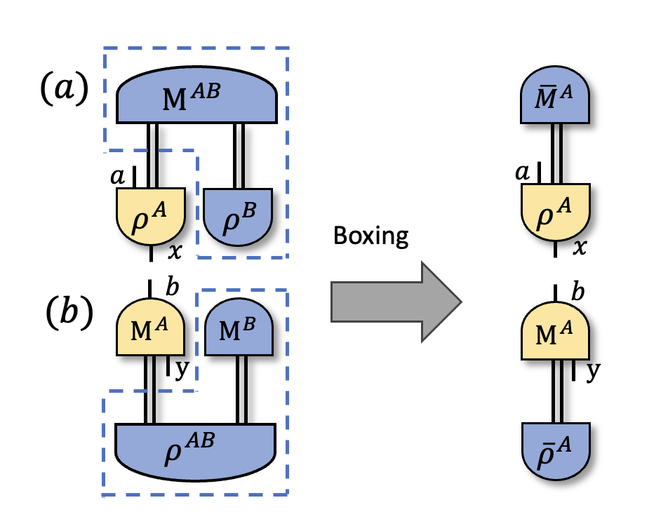
Figure 3: Left: Probing schemes (in blue) that can generate statistics that are not classically explainable independently of the identity of the given process of interest (in yellow). In (a), the process of interest is a multi-source. In (b), the process of interest is a multi-measurement. Right: Treating these same circuits in a manner that coarse-grains over all processes involving systems that are not connected directly to the process of interest leads to probing schemes (in blue) such that whether the statistics can be explained classically now always depends nontrivially on the identity of the process of interest. In (a), the effective process is simply an effect $\bar{M}^{A}$; in (b), the effective process is simply a state $\bar{\rho}^{A}$.

Similarly, consider the question of whether a given multi-measurement is nonclassical. Suppose one has the circuit in Figure 3(b), where the multi-measurement appears in yellow, and suppose that the composite of system and ancilla is prepared in some joint state (in blue) and subsequently a factorizing measurement is made, with some local measurement implemented on the ancilla. Again, it is possible to observe nonclassicality regardless of the identity of the multi-measurement on the system: simply take the joint state to be factorizing across the system-ancilla divide, and choose any set of states and set of effects on the ancilla sufficient to generate statistics that are nonclassical (in the sense of Definition 1).

In both cases then, one cannot conclude that the process in question is implicated in the fact that the overall circuit admits of no classical explanation.

To ensure that the lack of classical explainability of the circuit implicates the nonclassically of the process of interest, it suffices to stipulate that when assessing representability by an ontological model, one cannot appeal to any causal structure within the embedding circuit—one must rather box together (i.e., compose together) all quantum processes on any ancillary quantum systems that were introduced in the embedding circuit. In the above examples, this entails boxing together the blue processes to define an effective process: in Figure 3(a), one must compose the effect $M^{AB}$ with the state $\rho^{B}$ to define an effective effect $\bar{M}^{A}$ on system $A$ alone; in Figure 3(b), one must compose the effect $M^{B}$ with the state $\rho^{AB}$ to define an effective state $\bar{\rho}^{A}$ on system $A$ alone. By boxing processes in this manner, one ensures that any nonclassicality in the circuit comes from constraints pertaining to the system of interest (here, system $A$), as opposed to any ancilla systems introduced in the circuit (here, system $B$).

Equivalently, one can simply define nonclassicality of a given process in terms of whether or not it can generate nonclassical statistics when embedded in a circuit that does not introduce any new quantum systems. That is, the circuit cannot contain any quantum systems not connected directly to the process itself (for instance, it cannot contain a system such as $B$ in Figure 3). This is consistent with the fact that noncontextuality is always defined relative to some specified systems. Consequently, one wishes to consider the possibility of classical explanations for the systems in question (those connected to the given process) and no others, and the stipulation just given is a simple heuristic to guarantee this.

We formalize all this by defining the notion of a dual process to $P$.

Definition 2.

For a given type of quantum process $P$, a dual process to $P$ is a quantum process that has a quantum input corresponding to every quantum output of $P$ and a quantum output corresponding to every quantum input of $P$, and that has no other inputs or outputs.

If one connects (that is, one “wires together”) each quantum output of $P$ to the corresponding quantum input of the dual process and each quantum input of $P$ to the corresponding quantum output of the dual process, one obtains a circuit with no open quantum wires and with which one can associate a probability (for each value of the setting variables and outcome variables of the process $P$). It follows that a dual process defines a linear functional on the process $P$. We will refer to this wiring together of $D$ and $P$ to form $D\circ P$ as contracting $D$ with $P$.

We depict examples of dual processes in Figure 4. For a state, multi-state, source, or multi-source on system $A$, the dual process is an effect on $A$. Similarly, for an effect, measurement, or multi-measurement on system $A$, the dual process is a state on $A$.

Throughout the paper, we treat the variability in the states and effects of a dual process as theoretical variability (as discussed in Sec. II.3). Consequently, dual processes in our treatment have neither classical inputs nor classical outputs. As discussed in Sec. II.3, there are many different ways of ranging over all dual processes of a given type through physical variability (i.e., by the variability in the values of classical inputs and classical outputs), but the definition of classicality is independent of the choice of how to do so. This is discussed further in Appendix B.1.

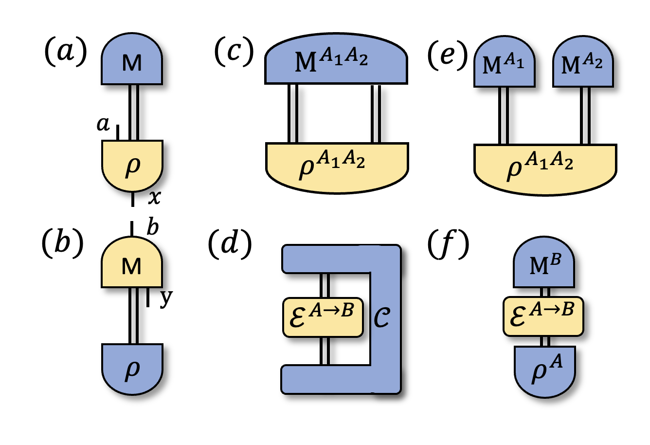
Figure 4: In (a)-(d), we depict examples of various types of processes (in yellow) and the associated dual processes (in blue). In (a), the process is a multi-source on a single system. In (b), it is a multi-measurement on a single system. In (c), it is a state on a bipartite system. In (d), it is a channel. In (e) and (f), the processes are the same as in (c) and (d) respectively, but we depict the associated dual processes when the latter are factorizing.

For a state on a multipartite system, the dual process is an effect on that multipartite system, as depicted in Fig. 4(a). The same is true if one considers a multi-state, source, or multi-source. For processes with both nontrivial quantum inputs and nontrivial quantum outputs, the dual process is a comb [73, 78], as depicted in Fig. 4 (d).

With these notions in hand, we can present our proposed notion of classicality for an individual process.

Definition 3.

A quantum process is classical if and only if the statistics generated by the set of circuits that contract the process of interest with any dual process (i.e., where the set ranges over all choices of dual process) are classically explainable (in the sense of Definition 1).

It is useful to provide a slightly more formal version of this definition. Suppose T denotes a process type, such as a preparation on $A$, a preparation on $AB$, a measurement on $A$, a transformation from $A$ to $B$, etcetera. For a process $P$ of type T, let the set of all processes of the dual type be denoted ${\rm AllDuals}(\texttt{T})$, and recall that the circuit one obtains by contracting a process $P$ with a dual process $D$ is denoted $D\circ P$. Relative to these notational conventions, the definition can be summarized as follows: a quantum process $P$ is classical if and only if the statistics generated by the set of circuits $\{D\circ P|D\in{\rm AllDuals}(\texttt{T})\}$ are classically explainable.

Note that this basic definition generalizes naturally to theories beyond quantum theory; that is, to arbitrary GPTs. However, in this work we focus on quantum theory specifically, and so we can simplify the definition considerably.

It turns out that it is sufficient to focus on a special class of dual processes. To define this class, we introduce the notion of a factorizing process.

Definition 4.

Recall that the type of a process specifies its inputs and outputs. A process is termed factorizing if it consists of a product of local effects on its quantum inputs and a product of local states on its quantum outputs.

A few examples serve to illustrate the idea. A state on a bipartite system $AB$ is factorizing if it is a product of a state on $A$ and a state on $B$. A process with quantum inputs $A$ and $B$ and a single quantum output $C$ is factorizing if it is a product of an effect on $A$ and an effect on $B$, composed sequentially with a state on $C$. A comb with quantum output $A$ and quantum input $B$ is factorizing if it consists of a state on $A$ and an effect on $B$.

With this definition, we prove (in Appendix C) the following.

Theorem 1.

If a quantum process is such that there exists some set of dual processes that it can be contracted with to obtain statistics that are not classically explainable, then there exists some set of factorizing dual processes for which this is the case.

Consequently, we can restrict our attention to factorizing dual processes, and we can in particular define the classical-nonclassical divide for a single quantum process as follows.

Definition $3^{\prime}$.

A quantum process is classical if and only if the statistics generated by the set of circuits that contract the process of interest with any factorizing dual process (i.e., where the set ranges over all choices of factorizing dual process) are classically explainable (in the sense of Definition 1).

This is the central definition of our manuscript.

IV Processes of the preparation or measurement variety

Let us start by reviewing the form of a classical explanation (an ontological model) for an entire prepare-measure scenario. We will consider the most general circuit in such a scenario, wherein there is a multi-source on the preparation side and a multi-measurement on the measurement side.

IV.1 Classical explainability of a prepare-measure scenario

Specifically, we consider a multi-source $\mathsf{P}\coloneqq\{\mathsf{P}_{x}\}_{x}\coloneqq\{\{p(a|x)\rho_{a|x}\}_{a}\}_{x}$ and a multi-measurement $\mathsf{M}\coloneqq\{\mathsf{M}_{y}\}_{y}\coloneqq\{\{M_{b|y}\}_{b}\}_{y}$, which generate the statistics

$$p(ab|xy)=p(a|x)\textrm{Tr}[M_{b|y}\rho_{a|x}]$$ (12)

when contracted together (as depicted in Fig. 5).

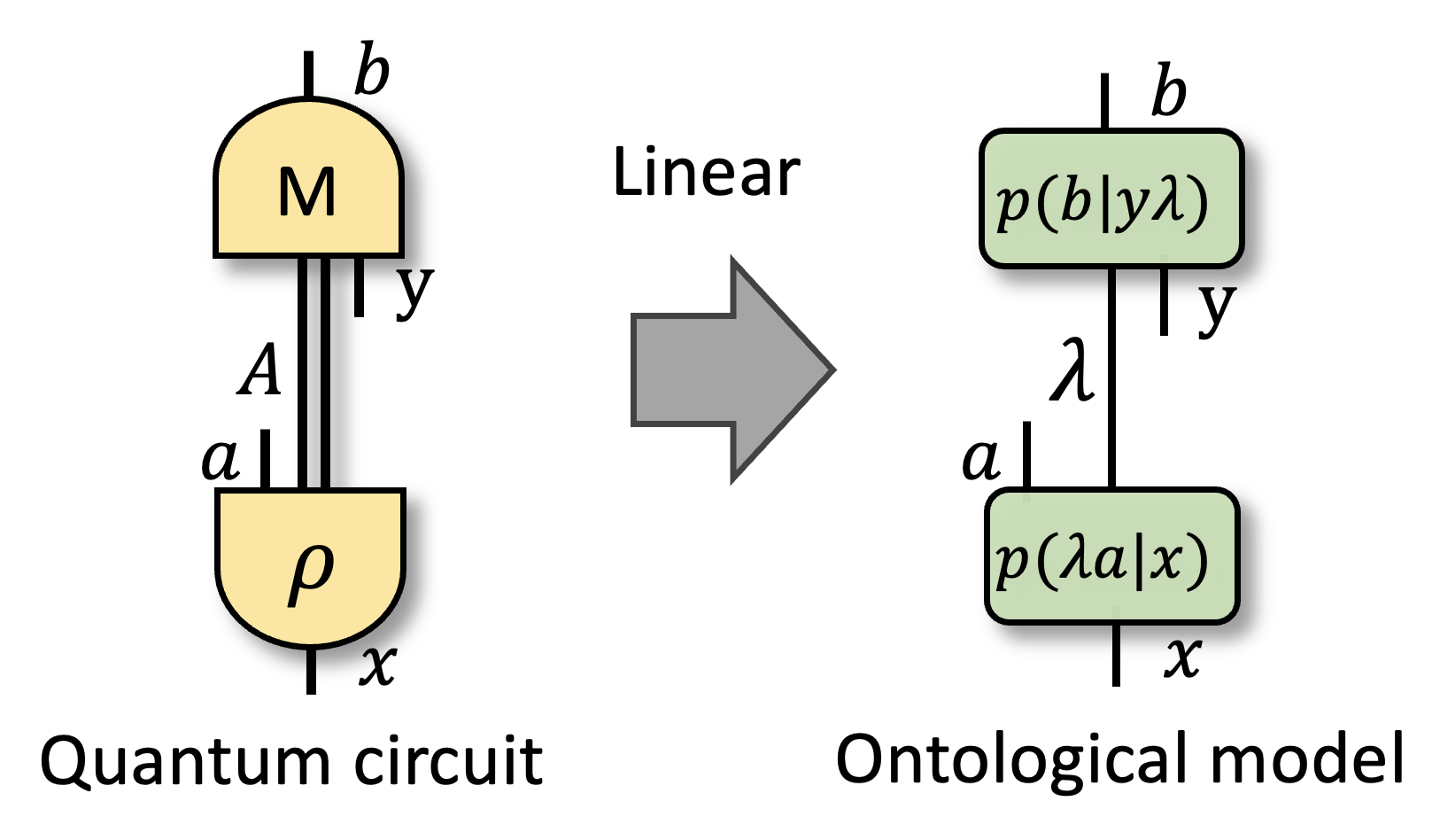
Figure 5: A prepare-measure circuit (left) and an ontological model for it (right).

The states and effects in such a circuit satisfy operational identities. We will identify these operational identities by their coefficients, and so we can denote the set of all operational identities for the states and that for the effects respectively by

$${{\mathcal{O}}_{\mathsf{P}}:=\{\{{\alpha}_{ax}\}_{ax}|\sum_{ax}{\alpha}_{ax}p(a|x){\rho}_{a|x}=0\}}$$ (13a)

$$\mathcal{O}_{\mathsf{M}}:=\{\{\alpha_{by}\}_{by}|\sum_{by}\alpha_{by}M_{b|y}=0\}.$$ (13b)

(Note that a simple method for characterizing and finding operational identities for an arbitrary set of states, effects, or transformations was introduced in Appendix A of Ref. [64].)

Consequently, this circuit is classically explainable (i.e., admits of a linear and diagram-preserving ontological representation) if and only if one can reproduce the quantum statistics as

$${p(ab|xy)=\sum_{\lambda}p(b|y\lambda)p(a\lambda|x)}$$ (14)

for some conditional probabilities $p(b|y\lambda)$ and $p(a\lambda|x)$ satisfying the ontological identities

$${\sum_{ax}{\alpha}_{ax}p(a\lambda|x)=0\quad\forall\{\alpha_{ax}\}_{ax}\in{\mathcal{O}}_{\mathsf{P}},}$$ (15a)

$$\sum_{by}\alpha_{by}p(b|y\lambda)=0\quad\forall\{\alpha_{by}\}_{by}\in\mathcal{O}_{\mathsf{M}}$$ (15b)

for all $\lambda$.

Note that these latter two constraints follow from linearity. In this simple context, the only constraints implied by diagram-preservation in this circuit are that states get represented as probability distributions, that effects get represented as response functions, and that the contraction of a state and an effect is represented as a probability, as in Eq. (14).

IV.2 The classical-nonclassical divide for multi-sources

Next, we characterize what states, multi-states, sources, and multi-sources are classical. Because all of these are special cases of the single concept of a multi-source, it suffices to define classicality for the latter. This is just a special case of Definition $3^{\prime}$:

Definition 5.

A multi-source is classical if and only if the statistics generated by the set of circuits that contract it with any effect (i.e., where the set ranges over all possible choices of effects) are classically explainable (in the sense of Definition 1).

The contraction of a multi-source with an effect results in a circuit of the prepare-and-measure form, as depicted in Fig. 4(a).

Precisely which multi-sources are classical is characterized by the following theorem.

Theorem 2.

A multi-source $\mathsf{P}\coloneqq\{\{p(a|x)\rho_{a|x}\}_{a}\}_{x}$ is classical (in the sense of Definition 5) if and only if it satisfies the following equivalent conditions:
(1) Each of the unnormalized states $p(a|x)\rho_{a|x}$ can be decomposed as

$${p(a|x)\rho_{a|x}=\sum_{\lambda}p(a\lambda|x)\sigma_{\lambda}\quad\forall a,x}$$ (16)

for some fixed set of normalized states $\{\sigma_{\lambda}\}_{\lambda}$ and some conditional probability distribution $p(a\lambda|x)$ satisfying

$${\sum_{ax}\alpha_{ax}p(a\lambda|x)=0\qquad\forall\{\alpha_{ax}\}_{a,x}\in\mathcal{O}_{\mathsf{P}}}$$ (17)

for all $\lambda$, where $\mathcal{O}_{\mathsf{P}}$ is defined in Eq. (13a).
(2)Each of the normalized states $\rho_{a|x}$ can be decomposed within a frame representation on span $V=\text{Span}\{\rho_{a|x}\}$ as

$$\rho_{a|x}=\sum_{\lambda}\textrm{Tr}[H_{\lambda}\rho_{a|x}]\sigma_{\lambda},\quad\forall a,x$$ (18)

where the set of frame operators is a fixed set of density operators $\{\sigma_{\lambda}\}_{\lambda}$ and the dual frame is a set of Hermitian operators $\{H_{\lambda}\}_{\lambda}$ satisfying $\sum_{\lambda}H_{\lambda}=\mathbb{1}_{V}$ and $\textrm{Tr}[H_{\lambda}\rho_{a|x}]\in[0,1]$ for all $a,x,\lambda$.

The proof is given in Appendix D. We will sometimes refer to this result as a structure theorem for nonclassical multi-sources.

In a companion paper [70], we leverage this theorem to provide detailed results on the certification and quantification of the nonclassicality of general states.

We can also derive some immediate insights from this theorem. First, consider multi-sources that arise in quantum steering [79, 80] experiments. As shown on the left-hand side of Figure 6, a pair of systems, $A_{1}$ and $A_{2}$ are prepared in an entangled state, and a multi-measurement is implemented on $A_{1}$. This yields an effective process that is a multi-source on $A_{2}$. Such a multi-source always satisfies $\sum_{a}p(a|x)\rho_{a|x}=\sigma$ for some state $\sigma$ independent of $x$, and is typically termed an assemblage [81]. An assemblage is said to be unsteerable [79] if its unnormalized states can be decomposed as

$$p(a|x)\color[rgb]{0,0,0}\rho_{a|x}=\sum_{\lambda}p(\lambda)p(a|x\lambda)\sigma_{\lambda},$$ (19)

for some set $\{\sigma_{\lambda}\}_{\lambda}$ of density operators on $A_{2}$, some probability distribution $p(\lambda)$, and some conditional probability distribution $p(a|x\lambda)$, as depicted in Figure 6. This is often termed a local hidden state model of the assemblage. (Note that in the resource theory of Local Operations and Shared Randomness [82, 1, 2, 3], the unsteerable assemblages are the free resources when one considers processes corresponding to a steering experiment [83, 84].) If an assemblage fails to satisfy the condition for being unsteerable, it is said to be steerable.

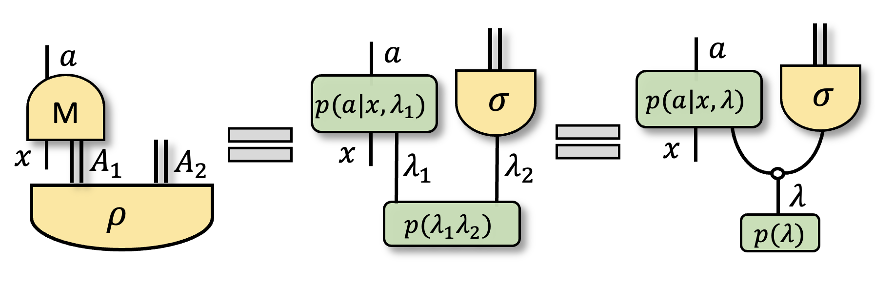
Figure 6: A steering experiment defines a multi-source $\{\{p(a|x)\rho_{a|x}\}_{a}\}_{x}$, often termed an assemblage. An assemblage is said to be unsteerable (or free) if and only if it admits of a decomposition in terms of Local Operations and Shared Randomness, as $\sum_{\lambda_{1},\lambda_{2}}p(a|x\lambda_{1})p(\lambda_{1}\lambda_{2})\sigma_{\lambda_{2}}$, as shown in the middle figure, or equivalently, as $\sum_{\lambda}p(\lambda)p(a|x\lambda)\sigma_{\lambda}$, as shown in the right-hand figure.

Given the definition of steerability, Theorem 2 immediately implies the following result.

Lemma 1.

Every steerable assemblage is nonclassical.

Proof.

We prove the contrapositive that if the multi-source defined by an assemblage is classical, then it is unsteerable. The assumption of classicality is given by condition (1) of Theorem 2. Summing Eq. (80) over the $a$ index, and using the fact that an assemblage satisfies $\sum_{a}p(a|x)\rho_{a|x}=\sigma$ for some $\sigma$, we obtain

$$\sum_{\lambda}p(\lambda|x)\sigma_{\lambda} =\sigma.$$ (20)

One can conceptualize $p(\lambda|x)$ as the ontological representation of $\sigma$. Linearity then implies that $p(\lambda|x)$ must have a trivial $x$ dependence, i.e.,

$$p(\lambda|x)=p(\lambda).$$ (21)

By Bayesian inversion,

$$p(a\lambda|x)=p(a|x\lambda)p(\lambda|x),$$ (22)

and so Eq. (21) implies

$$p(a\lambda|x)=p(a|x\lambda)p(\lambda).$$ (23)

Plugging this into Eq. (80), we obtain Eq. (19), the condition for being an unsteerable assemblage. ∎

In other words, an assemblage being classical (in the sense of Definition 3) implies that it admits of a local hidden state model and that it is a free resource relative to Local Operations and Shared Randomness. Note, however, that the converse is not true, as is established below in Example 2.

Theorem 2 also has consequences for the particular case of a multi-state where the states are linearly independent. For any multi-state described by a set $\{\rho_{\cdot|x}\}_{x}$ of linearly independent states on a single system, the set $\mathcal{O}_{P}$ of operational identities it satisfies is empty, so (by Eq. (81)) there are no constraints on the set of distributions $\{p(\lambda|x)\}_{x}$ that are the ontological representations of these. Consequently, one can always find a decomposition as in Eq. (80) (where $a$ is trivial) by defining $\sigma_{\lambda}:=\rho_{\lambda}$ and $p(\lambda|x)=\delta_{x,\lambda}$. So one has the following result (also noted in Ref. [68]):

Lemma 2.

Any set of linearly independent states on a single system is classically explainable.

From this, one can prove that any set of three or fewer states on a single system is also classical. (The classical explainability of a prepare-measure scenario involving fewer than four states was first noted in Ref. [85].) The case where the states are linearly independent is covered by Lemma 2, so it suffices to consider the case where they are linearly dependent. The single state case is trivial. For a pair of states, linear dependence implies that the states are equal, so we again have a trivial case. For a triple of states, any possible linear dependence has the form $\rho_{3}=p\rho_{1}+(1-p)\rho_{2}$ for some $p\in[0,1]$. There is consequently a single operational identity in the set $\mathcal{O}_{P}$. But in this case, one can find a decomposition as in Eq. (80), where $a$ is trivial, where $\Lambda:=\{1,2\}$, where $\sigma_{1}:=\rho_{1}$ and $\sigma_{2}:=\rho_{2}$, and where $p(\lambda|x)=\delta_{x,\lambda}$ for $x\in\{1,2\}$ and $p(\lambda|x)=p\delta_{\lambda,1}+(1-p)\delta_{\lambda,2}$ for $x=3$. The last equation ensures that Eq. (81) is satisfied and hence that condition (1) of Theorem 2 holds.

This argument generalizes to give the following sufficient condition for classicality of a set of states.

Corollary 1.

If a set of states fits inside a simplex within the quantum state space, then it is classical.

This is proven in Appendix F.

For a set of distinct pure states, linear dependence is not only necessary for nonclassicality (per lemma 2), but also sufficient.

Corollary 2.

A set of distinct pure states on a single system is classically explainable if and only if they are linearly independent.

The proof is in Appendix G.

So, for example, any set of five pure states of a qubit are nonclassical, as are any four pure states lying within a plane of the Bloch ball.

An example of such a set of four states arises in the BB84 protocol [86] and in parity-oblivious multiplexing [41]:

Example 1.

The set of states $\{|0\rangle,|1\rangle,|+\rangle,|-\rangle\}$ is nonclassical.

As proven in Ref. [29], the qualitative nonclassicality of a set of states is not affected by rescaling those states by any numbers in $(0,1]$. Consequently, we can use the previous example to construct an unsteerable assemblage that is nonclassical.

Example 2.

The source $\mathsf{P}=\{p(a)\rho_{a}\}_{a}=\{\frac{1}{4}|0\rangle\langle 0|,\frac{1}{4}|1\rangle\langle 1|,\frac{1}{4}|+\rangle\langle+|,\frac{1}{4}|-\rangle\langle-|\}$ is nonclassical.

Considered as an assemblage, this is obviously unsteerable, since it has no setting variable (i.e., it is a single ensemble, rather than a set of ensembles) and Eq. 19 is satisfied trivially.

Note, however, that there exist classical sets of states that exhibit nontrivial linear dependence relations, and moreover that do not fit inside a simplex within the quantum state space. This is illustrated below in Example 3.

In a companion paper [70], we derive a semidefinite program for evaluating the nonclassicality of sets of states. It establishes the claim of nonclassicality in the following example.

Example 3.

Consider a set of states

$$\left\{\frac{1}{2}[\mathbb{1}+\eta\hat{n}_{x}]\right\}_{x},$$ (24)

where $\{\hat{n}_{x}\}$ are unit vectors corresponding to the eight vertices of a cube inscribed in the Bloch sphere. This set is classical if and only if $\eta\leq\frac{1}{\sqrt{3}}$. (See Ref. [70] for the proof.) However, these states are linearly dependent for all $\eta>0$; moreover, it can be verified geometrically that a shrunken cube with vertices $\{\frac{1}{\sqrt{3}}\hat{n}_{x}\}$ cannot be contained inside any tetrahedron that fits inside the Bloch sphere, and so the set of states when $\eta=\frac{1}{\sqrt{3}}$ does not fit inside any simplex within the quantum state space.

IV.3 The classical-nonclassical divide for multi-measurements

Next, we turn to measurements. Recall that we use the term “measurement” to refer to the retrodictive aspect of a device with a quantum input and a classical outcome, and we use the term “multi-measurement” to refer to the retrodictive aspect of such a device when it has a setting variable as well.

The definition of nonclassicality of a multi-measurement is again a special case of Definition $3^{\prime}$:

Definition 6.

A multi-measurement is classical if and only if the statistics generated by the set of circuits where it is contracted with any state (i.e., where the set ranges over all states) are classically explainable (in the sense of Definition 1).

Precisely which multi-measurements are classical can be tested in a prepare-and-measure circuit as depicted in Fig. 4(b) and is characterized by the following theorem.

Theorem 3.

A multi-measurement $\mathsf{M}=\{\{M_{b|y}\}_{b}\}_{y}$ is classical (in the sense of Definition 6) if and only if it satisfies the following equivalent conditions:
(1) Its effects can be decomposed as

$$M_{b|y}=\sum_{\lambda}p(b|y\lambda)G_{\lambda}\quad\forall b,y$$ (25)

where $\{G_{\lambda}\}_{\lambda}$ is a POVM and $p(b|y\lambda)$ is a conditional probability distribution respecting constraints coming from Eq. (13b), namely satisfying (for all $\lambda$)

$$\sum_{by}\beta_{by}p(b|\lambda,y)=0\qquad\forall\{\beta_{by}\}_{by}\in\mathcal{O}_{\mathsf{M}}.$$ (26)

(2) Its effects can be decomposed within a frame representation on span $V=\text{Span}\{M_{b|y}\}$ as

$$M_{b|y}=\sum_{\lambda}\textrm{Tr}[M_{b|y}F_{\lambda}]G_{\lambda}\quad\forall b,y$$ (27)

where $\{G_{\lambda}\}_{\lambda}$ is a POVM and $\{F_{\lambda}\}_{\lambda}$ is a set of Hermitian operators satisfying $\textrm{Tr}[F_{\lambda}]=1$ and $\textrm{Tr}[M_{b|y}F_{\lambda}]\in[0,1]$ for all $b,y,\lambda$.

This is proven in Appendix E. We will sometimes refer to this as a structure theorem for nonclassical multi-measurements.

It is worth noting that an alternative proof is possible by leveraging Theorem 2 and Lemma 4 from Section VII. Essentially, a multi-measurement defines a special type of multi-source (known as a steering assemblage) via the Choi-isomorphism, and Lemma 4 asserts that the verdict of nonclassicality is preserved under the Choi isomorphism. Conditions (1) and (2) here are the translations of conditions (1) and (2) of Theorem 2 under the Choi isomorphism.

Several interesting insights follow from this theorem (most of which are direct analogues of those in the previous section).

First, recall that a set of measurements is compatible [87] if and only if there is single measurements $\{G_{\lambda}\}_{\lambda}$ that can be post-processed to reproduce every measurements in the set. Representing this set of measurements as a multi-measurement, this implies that

$$M_{b|y}=\sum_{\lambda}p(b|y\lambda)G_{\lambda},$$ (28)

as depicted in Figure 7. Any set of measurements for which this is not possible is said to be incompatible.

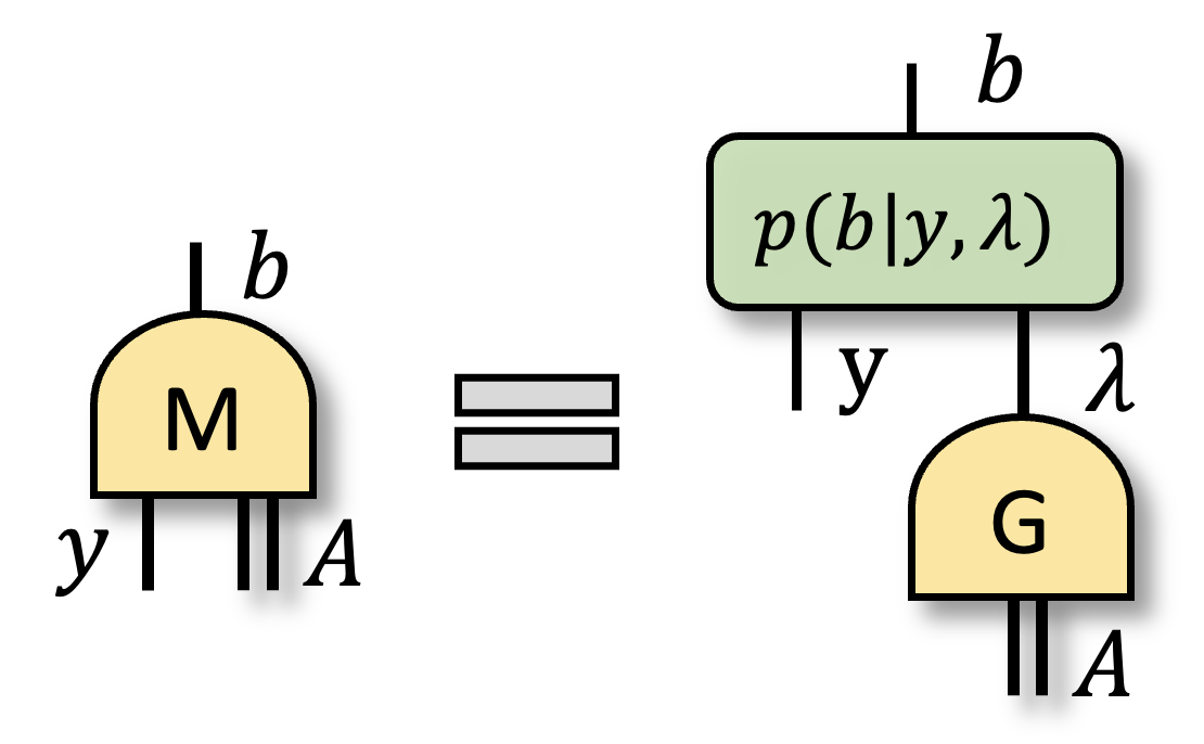
Figure 7: A set of measurements $\{\{M_{b|x}\}_{b}\}_{x}$ is compatible if and only if there is a single measurement which can be classically postprocessed to reproduce it. This implies that a multi-measurement ranging over those measurements decomposes as pictured (where the single measurement is labeled $G$).

Recalling this, Theorem 3 immediately implies the following.

Lemma 3.

Every set of incompatible measurements is nonclassical.

This follows from the form of Eq. (25), since the POVM $\{G_{\lambda}\}_{\lambda}$ defines a single measurement that can simulate all of the measurements in the given set via postprocessing [87]. However, due to the extra constraints in Eq. (26), there are sets of measurements that are all compatible and yet for which the set is nonetheless nonclassical.

A more exhaustive comparison between nonclassicality and incompatibility of a set of measurements is carried out in our companion paper [70].

The analogue of Corollary 2 for effects holds by an analogous proof:

Corollary 3.

A rank-1 POVM is classical if and only if its effects are linearly independent.

One significant implication of this corollary is that any rank-1 symmetric informationally-complete POVM is classical.

Unlike for a single state, a single measurement $\{M_{b}\}_{b}$ can be nonclassical, provided that there are nontrivial operational identities among its effects [88].

Example 4.

The family of noisy Pentagon measurements $\{M^{\eta}_{b}\}_{b=0}^{4}$ (defined for $\eta=1$ in Ref. [88]), where

$$M^{\eta}_{b}=\frac{1}{5}(\mathbb{1}+\eta(\cos\theta_{b}\sigma_{x}+\sin\theta_{b}\sigma_{z})]~~~\theta_{b}=\frac{2\pi b}{5},$$ (29)

is nonclassical if and only if $\eta\gtrapprox 0.618$, as we prove in Ref. [70].

V Processes of the bipartite preparation variety

Any single state on a unipartite system is classically explainable. This follows, in particular, from Lemma 2. However, once one considers multipartite systems, even a single state can be nonclassical. This is because subsystem structure provides new opportunities for witnessing nonclassicality (as first recognized in Ref. [68]).

When defining a linear and diagram-preserving ontological representation of a circuit that involves parallel composition of two or more systems (represented diagrammatically by a pair of wires), the assumption of diagram preservation implies that each system is associated with its own independent ontic state space. The ontic state space of the joint system is the Cartesian product of the ontic state spaces of the subsystems, an assumption that is sometimes called ontic separability.

If one instead wishes to entertain an ontological representation wherein the ontic state space of the joint system is not a Cartesian product, then one should rather represent the bipartite system in the quantum circuit as a single monolithic system—without a factorization into subsystems. In this case, the assumption of diagram-preservation would not force one to assume ontic separability. Under such a choice, the joint system would be treated as a unipartite system and represented diagramatically by a single wire rather than a pair.

Recall from Section II.2 that assessments of nonclassicality are always made relative to a given circuit, which effectively embodies a hypothesis about the causal structure. It should be clear from the previous paragraph that for a quantum system represented by a 4-dimensional Hilbert space, viewing it as (i) a single monolithic system or (ii) as a pair of qubits (according to some factorization of the system into a pair of 2-dimensional subsystems) constitutes two different hypotheses about the causal structure that are represented by different circuits. Indeed, the latter view (wherein a privileged factorization is specified for the full system) gives a more fine-grained perspective on the system. This is reflected by the fact that an ontological model associates to a monolithic system an ontic state space with no particular structure, while it associates to a bipartite system an ontic state space that has extra structure—it must be the Cartesian product of two ontic state spaces, one for each subsystem.

Assessments of nonclassicality may depend on which view of the system one takes. In particular, the unipartite view may lead to an assessment of classicality, while the bipartite view may lead to an assessment of nonclassicality. (Note that if the bipartite view leads to an assessment of classicality, then the unipartite view will as well.) Indeed, we will see this in the following results, where we show that any entangled state on a bipartite system is nonclassical relative to the specified bipartition, whereas we saw in Section IV.1 (from Lemma 2, for example) that any individual state is classical when it is conceptualized as a state on a unipartite system with no specified subsystem structure.

To discuss the nonclassicality of a bipartite state, one must consider the circuit obtained by contracting it with its dual process, which is a bipartite effect, as depicted in Fig. 4(c). Given Theorem 1, however, it suffices to consider the effects that factorize across the bipartition—hence, only local measurements. Thus, it suffices to consider only circuits that have the form depicted in Fig. 4(e).

V.1 Classical explainability of a prepare-measure scenario on a bipartite system with local measurements

As preparation for our discussion of nonclassicality of bipartite states, we consider the question of when a prepare-measure scenario involving a bipartite state and local measurements is classically explainable.

Specifically, we consider a circuit wherein the composite system $A_{1}A_{2}$ is prepared in a particular bipartite state $\rho^{A_{1}A_{2}}$ and then $A_{1}$ is subjected to a multi-measurement $\mathsf{M}_{1}$ while $A_{2}$ is subjected to a multi-measurement $\mathsf{M}_{2}$, where $\mathsf{M}_{i}\coloneqq\{\{M_{b_{i}|y_{i}}\}_{b_{i}}\}_{y_{i}}$. In such an experiment, depicted in Figure 8(a), quantum theory predicts that

$$p(b_{1}b_{2}|y_{1}y_{2})=\textrm{Tr}[\rho^{A_{1}A_{2}}M_{b_{1}|y_{1}}\otimes M_{b_{2}|y_{2}}].$$ (30)

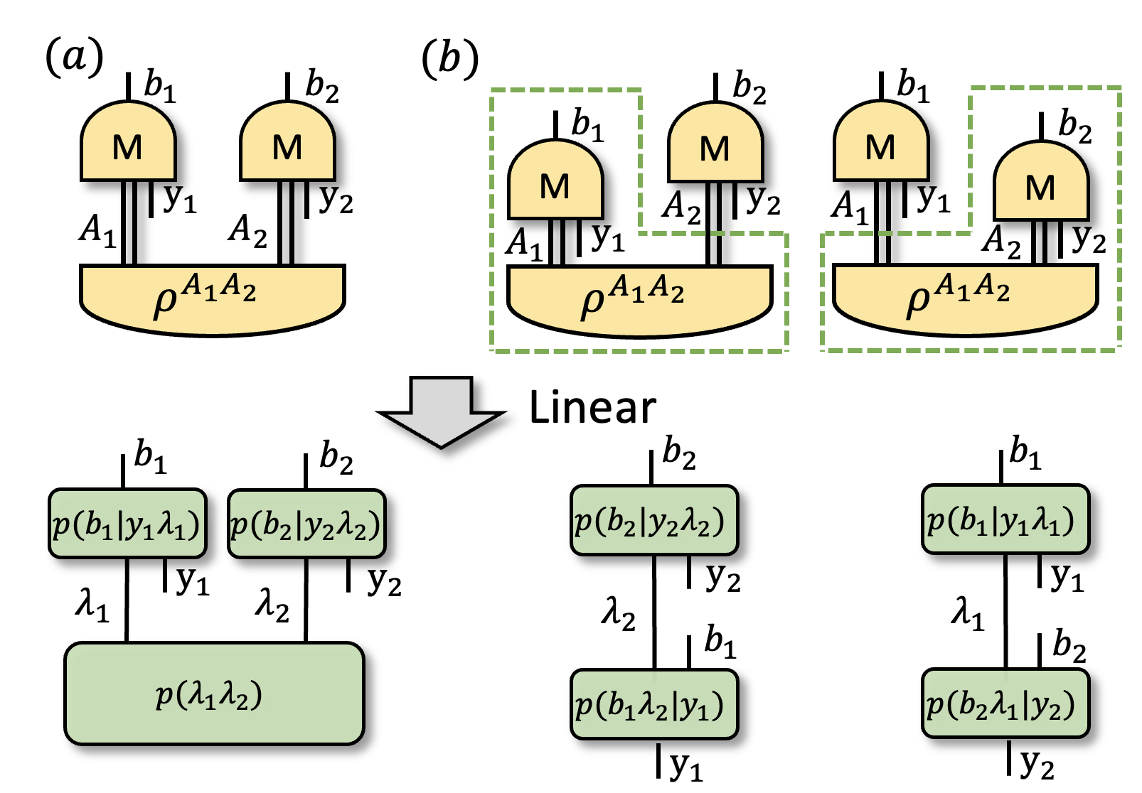
Figure 8: a) Local measurements on a bipartite state. b) By boxing processes together, we can view this circuit as a set of preparations and measurements on $B_{2}$, or as a set of preparations and measurements on $B_{1}$. In the top of the figure, we depict the quantum circuits; in the bottom, we depict an ontological model of each circuit.

There are no operational identities among bipartite states in this circuit, because it considers only a single (fixed) bipartite state. However, there are operational identities among the effects on each system, namely

$$\mathcal{O}_{\mathsf{M}_{1}}=\{\{\alpha_{b_{1}y_{1}}\}|\sum_{b_{1}y_{1}}\alpha_{b_{1}y_{1}}M_{b_{1}|y_{1}}=\mathbb{0}\},$$ (31a)

$$\mathcal{O}_{\mathsf{M}_{2}}=\{\{\alpha_{b_{2}y_{2}}\}|\sum_{b_{2}y_{2}}\alpha_{b_{2}y_{2}}M_{b_{2}|y_{2}}=\mathbb{0}\}.$$ (31b)

There are further operational identities in this circuit as a consequence of the fact that one can group together effects on system $$A_{1} A_{2} A_{2} A_{1}$$ with the multipartite state to define a set of states on , or group together effects on system with the multipartite state to define a set of states on , as shown in Figure 8(b). In particular, these operational identities are of the form

$$\mathcal{O}_{\mathsf{M}_{1}\circ\mathsf{P}}=\{\{\alpha_{b_{1}y_{1}}\}|\sum_{b_{1}y_{1}}\alpha_{b_{1}y_{1}}\textrm{Tr}_{A_{1}}[M_{b_{1}|y_{1}}\otimes\mathbb{1}_{2}\rho^{A_{1}A_{2}}]=\mathbb{0}\}$$ (32a)

$$\mathcal{O}_{\mathsf{M}_{2}\circ\mathsf{P}}=\{\{\alpha_{b_{2}y_{2}}\}|\sum_{b_{2}y_{2}}{\alpha}_{b_{2}y_{2}}\textrm{Tr}_{A_{2}}[\mathbb{1}_{1}\otimes M_{b_{2}|y_{2}}\rho^{A_{1}A_{2}}]=\mathbb{0}\}.$$ (32b)

Note that these last two equations actually subsume Eq. (31a) and Eq. (31b), respectively, in the sense that $\mathcal{O}_{\mathsf{M}_{1}}\subseteq\mathcal{O}_{\mathsf{M}_{1}\circ\mathsf{P}}$ and $\mathcal{O}_{\mathsf{M}_{2}}\subseteq\mathcal{O}_{\mathsf{M}_{2}\circ\mathsf{P}}$, since $\sum_{b_{1}y_{1}}\alpha_{b_{1}y_{1}}M_{b_{1}|y_{1}}=\mathbb{0}$ implies $\sum_{b_{1}y_{1}}\alpha_{b_{1}y_{1}}\textrm{Tr}_{1}[M_{b_{1}|y_{1}}\otimes\mathbb{1}_{2}\rho^{A_{1}A_{2}}]=\mathbb{0}$.

Consequently, this circuit is classically explainable (i.e., admits of an ontological model) if and only if one can introduce a separable ontic state space $\Lambda_{1}\times\Lambda_{2}$ over which one can reproduce the quantum statistics via

$$p(b_{1}b_{2}|y_{1}y_{2})=\sum_{\lambda_{1}\lambda_{2}}p(\lambda_{1}\lambda_{2})p(b_{1}|y_{1}\lambda_{1})p(b_{2}|y_{2}\lambda_{2}),$$ (33)

where $p(b_{1}|y_{1}\lambda_{1})$ respects the identities implied by $\mathcal{O}_{\mathsf{M}_{1}}$, where $p(b_{2}|y_{2}\lambda_{2})$ respects the identities implied by $\mathcal{O}_{\mathsf{M}_{2}}$, where the composite $\sum_{\lambda_{1}}p(b_{1}|y_{1}\lambda_{1})p(\lambda_{1}\lambda_{2})$ respects the identities implied by $\mathcal{O}_{\mathsf{M}_{1}\circ\mathsf{P}}$, and where the composite $\sum_{\lambda_{2}}p(b_{2}|y_{2}\lambda_{2})p(\lambda_{1}\lambda_{2})$ respects the identities implied by $\mathcal{O}_{\mathsf{M}_{2}\circ\mathsf{P}}$; explicitly, we require, for all $\lambda_{1},\lambda_{2}$,

$$\sum_{b_{1}y_{1}}\alpha_{b_{1}y_{1}}p(b_{1}|y_{1}\lambda_{1})=0\quad\forall\{\alpha_{b_{1}y_{1}}\}\in\mathcal{O}_{\mathsf{M}_{1}}$$ (34a)

$$\sum_{b_{2}y_{2}}\alpha_{b_{2}y_{2}}p(b_{2}|y_{2}\lambda_{2})=0\quad\forall\{\alpha_{b_{2}y_{2}}\}\in\mathcal{O}_{\mathsf{M}_{2}}$$ (34b)

$$\sum_{b_{1}y_{1}}\alpha_{b_{1}y_{1}}\sum_{\lambda_{1}}p(b_{1}|y_{1}\lambda_{1})p(\lambda_{1}\lambda_{2})=0\quad\forall\{\alpha_{b_{1}y_{1}}\}\in\mathcal{O}_{\mathsf{M}_{1}\circ\mathsf{P}}$$ (34c)

$$\sum_{b_{2}y_{2}}{\alpha}_{b_{2}y_{2}}\sum_{\lambda_{2}}p(b_{2}|y_{2}\lambda_{2})p(\lambda_{1}\lambda_{2})=0\quad\forall\{\alpha_{b_{2}y_{2}}\}\in\mathcal{O}_{\mathsf{M}_{2}\circ\mathsf{P}}.$$ (34d)

Note that the first two constraints here follow from linearity, while the latter two follow from diagram-preservation together with linearity.

Moreover, one can write $\sum_{\lambda_{1}}p(b_{1}|y_{1}\lambda_{1})p(\lambda_{1}\lambda_{2})=p(b_{1}\lambda_{2}|y_{1})$, and $\sum_{\lambda_{2}}p(b_{2}|y_{2}\lambda_{2})p(\lambda_{1}\lambda_{2})=p(b_{2}\lambda_{1}|y_{2})$ since $b_{1}$ ($b_{2}$) is conditionally independent of $\lambda_{2}$ ($\lambda_{1}$) given $\lambda_{1}$ ($\lambda_{2}$). This leads to the very helpful proposition:

Proposition 1.

Any circuit with local measurements on a bipartite state (as depicted in Fig. 8(a)) is classically explainable only if the two prepare-measure circuits it induces by boxing processes together (in one or the other direction, as in Fig. 8(b)) are classically explainable.

This is proven in Appendix H. The implication is depicted in Fig. 8.

V.2 The classical-nonclassical divide for bipartite states

We obtain the definition of classicality for a single bipartite state by particularizing Definition $3^{\prime}$ to this type of process:

Definition 7.

A state on a bipartite system is classical if and only if the statistics generated by the set of circuits where it is contracted with any product effect (i.e., where the set ranges over all product effects) is classically explainable (in the sense of Definition 1).

We are led therefore to consider a prepare-measure circuit of the type depicted in Fig. 8(a), with a single bipartite state and measurements that factorize across the bipartition, but where the range of measurements includes every possible effect on $A_{1}$ and every possible effect on $A_{2}$, as depicted in Fig. 4(e).

A characterization of the nonclassical bipartite states can be obtained as a simple corollary of Proposition 1.

Theorem 4.

A bipartite state $\rho^{A_{1}A_{2}}$ is classical if the set of states on $A_{2}$ to which one steers by contracting with the set of all effects on $A_{1}$ is classical and the set of states on $A_{1}$ to which one steers by contracting with the set of all effects on $A_{2}$ is classical.

The proof is simple. If, for the bipartite state, every measurement on one system steers to the other system to a classical set of states, then, both prepare-measure circuits one can induce by boxing processes as in Figure 8 will be classically explainable. By Proposition 1, this implies that the prepare-measure circuit involving the bipartite state and all effects that factorize across the bipartition is classically explainable. By Definition 7, this in turn implies that the bipartite state is classical.

Whether the classicality of the set of steered states on both sides is sufficient to establish the classicality of the bipartite state is still unknown.

Note that in general, it may be possible to steer a state to a nonclassical set of states in one direction, but not the other. (This is illustrated by Example 5 below.)

It is easy to see that entanglement implies nonclassicality in the sense of Definition 7.

Proposition 2.

If a bipartite state is entangled, then it is nonclassical.

Proof.

We prove the contrapositive, that if a bipartite state is classical (in the sense of Definition 7), then it is separable. If $\rho^{A_{1}A_{2}}$ satisfies Definition 7, then its quantum statistics for all product effects $\{M_{1}^{A_{1}}\otimes M_{2}^{A_{2}}\}$ admit an ontological model with

$$\textrm{Tr}[M_{1}^{A_{1}}\otimes M_{2}^{A_{2}}\rho^{A_{1}A_{2}}]=\sum_{\lambda_{1}\lambda_{2}}p(\lambda_{1}\lambda_{2})p(M_{1}^{A_{1}}|\lambda_{1})p(M_{2}^{A_{2}}|\lambda_{2})$$ (35)

where $p(M_{i}^{A_{i}}|\lambda)$s depends linearly on the effect $M_{i}^{A_{i}}\in\mathcal{M}(\mathcal{H}^{A_{i}})$. Thus, from the generalized Gleason theorem [89], there exists a unique set of density matrices $\{\sigma^{A_{i}}_{\lambda_{i}}\}_{\lambda_{i}}$ such that $p(M_{i}^{A_{i}}|\lambda_{i})=\textrm{Tr}[M_{i}^{A_{i}}\sigma^{A_{i}}_{\lambda_{i}}]$, and so we have

$$\textrm{Tr}[M_{1}^{A_{1}}\otimes M_{2}^{A_{2}}\rho^{A_{1}A_{2}}]$$

$$= \sum_{\lambda_{1}\lambda_{2}}p(\lambda_{1}\lambda_{2})\textrm{Tr}[M_{1}^{A_{1}}\sigma^{A_{1}}_{\lambda_{1}}]\textrm{Tr}[M_{2}^{A_{2}}\sigma^{A_{2}}_{\lambda_{2}}]$$

$$= \textrm{Tr}[(M_{1}^{A_{1}}\otimes M_{2}^{A_{2}})\sum_{\lambda_{1}\lambda_{2}}p(\lambda_{1}\lambda_{2})\sigma^{A_{1}}_{\lambda_{1}}\otimes\sigma^{A_{2}}_{\lambda_{2}}]$$ (36)

Because the product effects span the set of all effects, this implies that

$$\rho^{A_{1}A_{2}}=\sum_{\lambda_{1}\lambda_{2}}p(\lambda_{1}\lambda_{2})\sigma^{A_{1}}_{\lambda_{1}}\otimes\sigma^{A_{2}}_{\lambda_{2}},$$ (37)

and so the state is separable. ∎

Just as entanglement, steering, and nonlocality are distinct bipartite resources[90, 91, 92, 93], the notion of a classical bipartite state introduced here is different from all of them. That is, while separability is a necessary condition for classicality, it is not sufficient, as demonstrated by the following example.

Example 5.

The separable bipartite state

$$\rho^{A_{1}A_{2}} =\frac{1}{4}(|0\rangle\langle 0|\otimes|0\rangle\langle 0|+|1\rangle\langle 1|\otimes|1\rangle\langle 1|$$ (38)

$$+|2\rangle\langle 2|\otimes|+\rangle\langle+|+|3\rangle\langle 3|\otimes|-\rangle\langle-|)$$ (39)

is nonclassical, because there exists a measurement on $A_{1}$, namely, the projector-valued measure $\{|0\rangle\langle 0|,|1\rangle\langle 1|,|2\rangle\langle 2|,|3\rangle\langle 3|\}$ that steers $A_{2}$ to the source $\{\frac{1}{4}|0\rangle\langle 0|,\frac{1}{4}|1\rangle\langle 1|,\frac{1}{4}|+\rangle\langle+|,\frac{1}{4}|-\rangle\langle-|\}$, which was shown to be nonclassical in Example 2.

Nonclassicality of a bipartite state, in the sense introduced here, also does not coincide with having nonzero discord [94]; for example, the state $\frac{1}{2}|0\rangle\langle 0|\otimes|0\rangle\langle 0|+\frac{1}{2}|1\rangle\langle 1|\otimes|+\rangle\langle+|$ has nonzero discord but is classical. It is not hard to see that nonzero discord is necessary but not sufficient for a single bipartite state to be nonclassical.

A complete characterization of the boundary between classical and nonclassical for bipartite states is likely to be difficult to obtain. For one, the set of classical bipartite states is not convex, because all product states are classical, but not all separable states are.

Still, one can find conditions that are helpful for witnessing the nonclassicality of a given state. We will give one such condition below, based on a property that some bipartite states possess which we term nonsingularness and that we define presently.

Definition 8.

A bipartite state $\rho^{A_{1}A_{2}}$ is nonsingular if and only if the steering maps induced by $\rho^{A_{1}A_{2}}$ are invertible. The steering maps are the superoperators $\Psi^{\rho}_{1}$ and $\Psi^{\rho}_{2}$ defined by the expressions

$$\Psi_{1}^{\rho}(X)=\textrm{Tr}_{A_{1}}[(X^{T}\otimes\mathbb{1}_{2})\rho^{A_{1}A_{2}}],$$ (40)

$$\Psi_{2}^{\rho}(X)=\textrm{Tr}_{A_{2}}[(\mathbb{1}_{1}\otimes X^{T})\rho^{A_{1}A_{2}}].$$ (41)

Equivalently, a bipartite state is nonsingular if it has no intrinsic operational identities, by which we mean that $\mathcal{O}_{\mathsf{M_{1}}\circ\mathsf{P}}=\mathcal{O}_{\mathsf{M_{1}}}$ and $\mathcal{O}_{\mathsf{M_{2}}\circ\mathsf{P}}=\mathcal{O}_{\mathsf{M_{2}}}$ where $\mathcal{O}_{\mathsf{M_{1}}}$, $\mathcal{O}_{\mathsf{M_{2}}}$, $\mathcal{O}_{\mathsf{M_{1}}\circ\mathsf{P}}$, and $\mathcal{O}_{\mathsf{M_{2}}\circ\mathsf{P}}$ are defined in Eqs. (31) and  (32) respectively, and where we are considering all effects on $A_{1}$ and all effects on $A_{2}$.

This equivalence can be easily seen from the fact that $\mathcal{O}_{\mathsf{M_{i}}\circ\mathsf{P}}$ in Eq. (32) can be expressed as

$$\mathcal{O}_{\mathsf{M_{i}}\circ\mathsf{P}}=\{\{\alpha_{b_{i}y_{i}}\}|\sum_{b_{i},y_{i}}\alpha_{b_{i}y_{i}}\Psi_{i}^{\rho}(M^{T}_{b_{i}|y_{i}})\}=0,$$ (42)

but by the invertibility of $\Psi_{i}^{\rho}$, this implies

$$\mathcal{O}_{\mathsf{M_{i}}\circ\mathsf{P}}=\{\{\alpha_{b_{i}y_{i}}\}|\sum_{b_{i},y_{i}}\alpha_{b_{i}y_{i}}M_{b_{i}|y_{i}}\}=0,$$ (43)

such that, recalling the definition of $\mathcal{O}_{\mathsf{M_{i}}}$ from Eqs. (31a) and  (31b), we infer that $\mathcal{O}_{\mathsf{M_{i}}\circ\mathsf{P}}=\mathcal{O}_{\mathsf{M_{1}}}$,

Corollary 4.

A nonsingular bipartite state is classical if and only if it is separable.

Proposition 2 establishes that separability is necessary for classicality for all bipartite states, so what remains to be proven is that for nonsingular bipartite states, it is also sufficient. For nonsingular bipartite states, $\mathcal{O}_{\mathsf{M_{i}}\circ\mathsf{P}}=\mathcal{O}_{\mathsf{M_{1}}}$, so one only needs to consider the first two sets of constraints in Eq. (34), which are of the form

$$\sum_{b_{i}}\alpha_{b_{i}}p(b_{i}|y_{i},\lambda_{i})=0~~~~\forall\{\alpha_{b_{i}}\}\in\mathcal{O}_{\mathsf{M_{i}}},$$ (44)

This is because the other two sets of constraints in Eq. (34c) and Eq. (34d), namely,

$$\sum_{b_{i}}\alpha_{b_{i}}\sum_{\lambda_{j\neq i}}p(\lambda_{i}\lambda_{j})p(b_{i}|y_{i},\lambda_{i})=0~\forall\{\alpha_{b_{i}}\}\in\mathcal{O}_{\mathsf{M_{i}}\circ\mathsf{P}},$$ (45)

are automatically satisfied since we have $\mathcal{O}_{\mathsf{M_{i}}\circ\mathsf{P}}=\mathcal{O}_{\mathsf{M_{i}}}$. Therefore, if only the first two sets of constraints need to be satisfied, once we can find the separable decomposition from Proposition 2 (which guarantees the first two sets of constraints), we can disregard the remaining two sets of constrains. Consequently, any nonsingular separable state under these conditions must be classical.

A Venn diagram depicting which bipartite states are nonclassical is presented in Fig. 9.

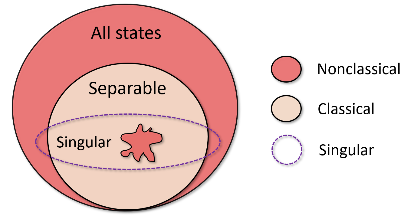
Figure 9: When considering bipartite quantum states: all entangled state are nonclassical; all nonsingular separable states are classically explainable; there exist singular separable states that are nonclassical; the set of classically explainable states is nonconvex. Notably, this schematic does not captures all the properties of these sets, in that the set of singular states should be measure zero, and it should contain all extremal separable states (i.e., the product states).

As discussed at the beginning of this section, diagram-preservation implies that an ontological model assigns a Cartesian product of ontic state spaces to a particular tensor product of Hilbert spaces. This leads to additional constraints on the ontological representation of quantum processes—constraints that can in turn imply nonclassicality of a process that would otherwise be judged classical. This highlights how conclusions about nonclassicality only hold relative to a choice of factorization of the Hilbert space. For instance, as noted above, a 4-dimensional Hilbert space can be factorized into a pair of 2-dimensional Hilbert spaces in many ways, where the factor spaces correspond to virtual subsystems [95]. Because for a given state there is always some choice of factorization relative to which it is entangled, it follows from Proposition 2 that there is always some choice of factorization relative to which it is nonclassical. In this article, the choice of factorization of Hilbert space relative to which nonclassicality is being judged is always specified by the circuit one is considering.

Note that the ideas and results in this section generalize straightforwardly to multipartite states, and that some of these generalizations appear in Section VII.

VI Processes of the transformation variety

To discuss the nonclassicality of a transformation, one must consider the circuit obtained by contracting the transformation with its dual process, namely, a comb, as depicted in Fig. 4(d). But given Theorem 1, we need not consider all combs. It suffices to consider those that factorize, meaning that they can be understood as a preparation preceding the transformation and a measurement following the transformation. In other words, it suffices to consider circuits that have the form depicted in Fig. 10(a), termed a prepare-transform-measure scenario.

As in the previous sections, we begin by reviewing the form of a classical explanation (i.e., a diagram-preserving and linear ontological representation) of a general prepare-transform-measure scenario.

VI.1 Classical explainability of a prepare-transform-measure scenario

We consider a multi-source $\mathsf{P}\coloneqq\{\{p(a|x)\rho_{a|x}\}_{a}\}_{x}$, followed by a channel ${\cal E}$, followed by a multi-measurement $\mathsf{M}=\{\{M_{b|y}\}_{b}\}_{y}$. (This is essentially a repeat of the example given in the preliminaries section, but with the state in that example being replaced by a multi-source.) For such a circuit, quantum theory predicts that

$$p(ab|xy)=p(a|x)\textrm{Tr}[M_{b|y}\mathcal{E}(\rho_{a|x})].$$ (46)

In this circuit, there are no operational identities among channels, as we consider only a single (fixed) channel. However, there are operational identities among the states on the input system and among the effects on the output system, namely

$$\mathcal{O}_{\mathsf{M}}=\{\{\alpha_{by}\}|\sum_{by}\alpha_{by}M_{b|y}=\mathbb{0}\},$$ (47a)

$$\mathcal{O}_{\mathsf{P}}=\{\{\alpha_{ax}\}|\sum_{a}\alpha_{ax}p(a|x)\rho_{a|x}=\mathbb{0}\}.$$ (47b)

There are also additional operational identities in this circuit, as a consequence of the fact that one can group the channel together with the states on its input to form some new set of (effective) states, or can group the channel together with effects on its output to define a new set of (effective) effects. These operational identities are of the form

$$\mathcal{O}_{\mathsf{M}\circ\mathcal{E}}=\{\{\alpha_{by}\}|\sum_{by}{\alpha}_{by}\mathcal{E}^{\dagger}(M_{b|y})=\mathbb{0}\},$$ (48a)

$$\mathcal{O}_{\mathcal{E}\circ\mathsf{P}}=\{\{\alpha_{ax}\}|\sum_{ax}{\alpha}_{ax}p(a|x)\mathcal{E}(\rho_{a|x})=\mathbb{0}\}.$$ (48b)

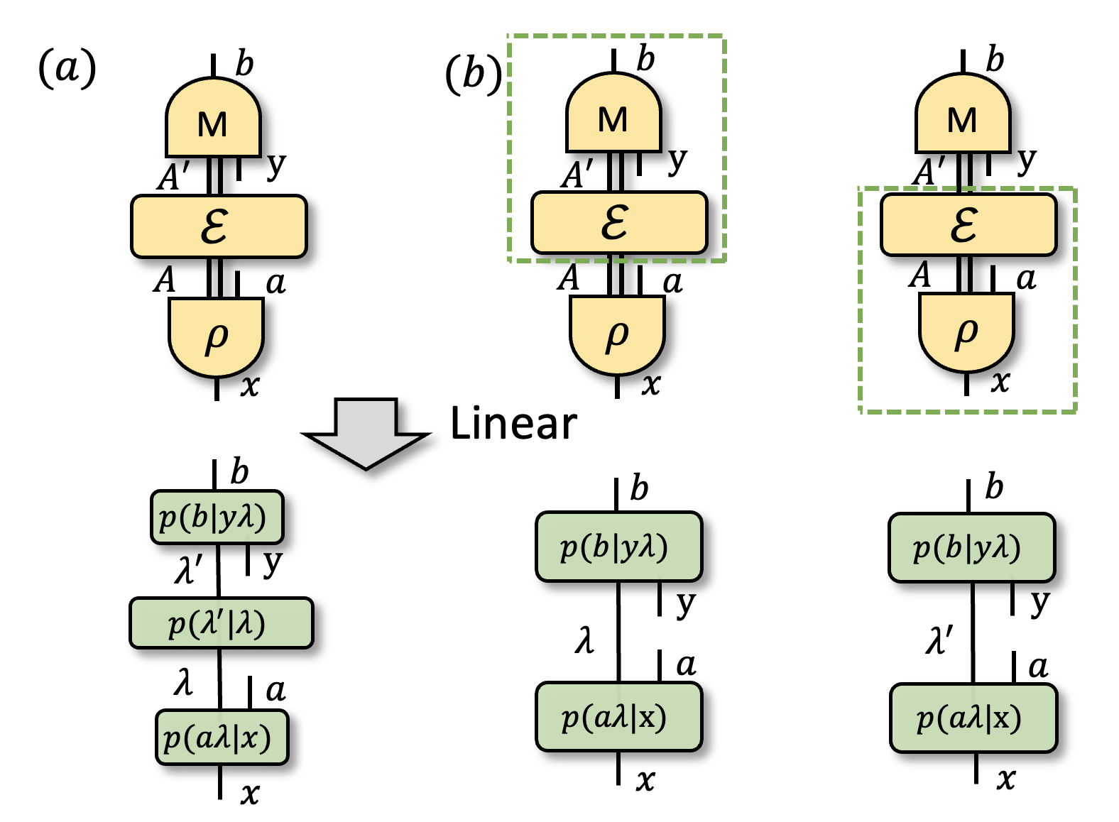
Figure 10: a) A prepare-transform-measure circuit. b) By boxing processes together, we can view this circuit as a set of preparations and measurements on system $A$, or as a set of preparations and measurements on system $A^{\prime}$. In the top of the figure, we depict the quantum circuits; in the bottom, we depict an ontological model of each circuit.

Consequently, a prepare-transform-measure circuit is classically explainable (i.e., admits of an ontological model) if and only if one can reproduce the quantum statistics via

$$p(ab|xy)=\sum_{\lambda\lambda^{\prime}}p(b|y\lambda^{\prime})p(\lambda^{\prime}|\lambda)p(a\lambda|x),$$ (49)

where $p(b|y\lambda^{\prime})$ respects the identities implied by $\mathcal{O}_{\mathsf{M}}$, where $p(a\lambda|x)$ respects the identities implied by $\mathcal{O}_{\mathsf{P}}$, where the composite $\sum_{\lambda^{\prime}}p(b|y\lambda^{\prime})p(\lambda^{\prime}|\lambda)$ respects the identities implied by $\mathcal{O}_{\mathsf{M}\circ\cal{E}}$, and where the composite $\sum_{\lambda}p(\lambda^{\prime}|\lambda)p(a\lambda|x)$ respects the identities implied by $\mathcal{O}_{{\cal E}\circ\mathsf{P}}$; explicitly, we require for all $\lambda,\lambda^{\prime}$,

$$\sum_{by}\alpha_{by}p(b|y\lambda^{\prime})=0\quad\forall\{\alpha_{by}\}\in\mathcal{O}_{\mathsf{M}},$$ (50a)

$$\sum_{ax}\alpha_{ax}p(a\lambda|x)=0\quad\forall\{\alpha_{ax}\}\in\mathcal{O}_{\mathsf{P}},$$ (50b)

$$\sum_{by}\alpha_{by}\sum_{\lambda^{\prime}}p(b|y\lambda^{\prime})p(\lambda^{\prime}|\lambda)=0\quad\forall\{\alpha_{by}\}\in\mathcal{O}_{\mathsf{M}\circ\cal{E}},$$ (50c)

$$\sum_{ax}{\alpha}_{ax}\sum_{\lambda}p(\lambda^{\prime}|\lambda)p(a\lambda|x)=0\quad\forall\{\alpha_{ax}\}\in\mathcal{O}_{{\cal E}\circ\mathsf{P}}.$$ (50d)

The first two constraints here follow from linearity, while the latter two follow from diagram-preservation together with linearity.

Finally, we present a result that will be useful for the characterization of nonclassical channels (the analogue of Proposition 1).

Proposition 3.

Any prepare-transform-measure circuit (as depicted in Fig. 10(a)) is classically explainable only if the two prepare-measure circuits it induces by boxing the transformations with the states or with the effects (the two cases depicted in Fig. 10(b)) are classically explainable.

VI.2 The classical-nonclassical divide for channels

We turn now to the definition of classicality for a channel, again obtained by particularizing Definition $3^{\prime}$. Recalling that the dual process of a channel from $A$ to $B$ is a comb with output $A$ and input $B$ and that a factorizing such comb constitutes a preparation on $A$ and a measurement on $B$, we are led to consider a prepare-transform-measure circuit of the type depicted in Fig. 10(a), but where the range of preparations includes every possible state on $A$ and the range of measurements includes every possible effect on $B$—a situation depicted in Fig. 4(f).

Definition 9.

A channel is classical if and only if the statistics generated by the set of circuits where it is contracted with any state at its input and any effect at its output (i.e., where the set ranges over all states and all effects) is classically explainable (in the sense of Definition 1).

A useful result concerning the class of nonclassical channels can be inferred from Proposition 3.

Theorem 5.

A channel is nonclassical if there exists a set of states whose image under the channel is nonclassical or there exists a set of effects whose image under the adjoint of the channel is nonclassical.

It is possible to give a proof that is analogous to that of Theorem 4. The result can also be understood as following from Theorem 4 by leveraging lemma. 4 (which will be presented in Section VII) because the latter result shows that the verdict regarding the nonclassicality of a channel is the same as that regarding its Choi-isomoprhic state.

Another useful characterization is the following.

Proposition 4.

If a channel is non-entanglement-breaking, then it is nonclassical.

This follows immediately from the fact that if a state of a bipartite system is entangled then it is nonclassical (Proposition 2) together with the fact that nonclassicality of processes is preserved under the Choi isomorphism (Lemma 4, which will be presented further on in the article). We give another simple proof of Proposition 4 in Appendix J.

Although being entanglement-breaking is a necessary condition for classicality, it is not sufficient, as illustrated by the following example.

Example 6.

The entanglement-breaking channel

$$\mathcal{E}(X) =\textrm{Tr}\big{[}|0\rangle\langle 0|X\big{]}|0\rangle\langle 0|+\textrm{Tr}\big{[}|1\rangle\langle 1|X\big{]}|1\rangle\langle 1|$$ (51)

$$+\textrm{Tr}\big{[}|2\rangle\langle 2|X\big{]}|+\rangle\langle+|+\textrm{Tr}\big{[}|3\rangle\langle 3|X\big{]}|-\rangle\langle-|$$

is nonclassical. This follows from Theorem 5 and the fact that if the input to the channel is the source $\{\frac{1}{4}|i\rangle\langle i|\}_{i=0}^{3}$, then its output is the source $\{\frac{1}{4}|0\rangle\langle 0|,\frac{1}{4}|1\rangle\langle 1|,\frac{1}{4}|+\rangle\langle+|,\frac{1}{4}|-\rangle\langle-|\}$, which is the nonclassical source discussed in Example 2. (Note that there does not exist a set of effects that is mapped by the adjoint of this channel to a nonclassical set of effects, since any set of effects will get mapped to a set of effects that are all diagonal in the same eigenbasis, namely, $\{|i\rangle\langle i|\}_{i=0}^{3}$.) An alternative proof of the nonclassicality of this channel is to note that the channel is Choi-isomorphic to the nonclassical separable state in Example 5 and to leverage the fact that nonclassicality is preserved under the Choi isomorphism (Lemma 4).

VII Processes of arbitrary type

In this section, we derive some results regarding the nonclassicality of a general process, and we ultimately show that the nonclassicality of any general process can be deduced by studying the nonclassicality of an associated multiparitite state:

Theorem 6.

For any given quantum process, consider the unique multipartite state associated to it by applying the Choi isomorphism to all of its quantum inputs, applying flag-convexification to all of its classical inputs, and then reconceptualizing all of its classical outputs as dephased quantum outputs. The process is nonclassical if and only if this associated multipartite state is nonclassical.

This follows from three lemmas.

The first lemma states that qualitative verdicts concerning the nonclassicality of a given process are preserved under the Choi isomorphism.

Lemma 4.

The Choi state isomorphic to a given process is nonclassical if and only if the process itself is nonclassical.

This is proven in Appendix K.

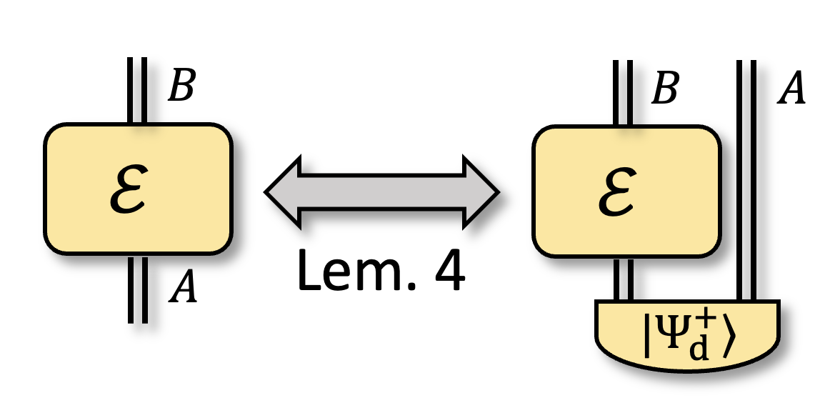
Figure 11: As an example of Lemma 4, a channel $\mathcal{E}^{A\rightarrow B}$ is nonclassical if and only if the Choi-isomorphic bipartite state $\rho^{BA}_{\mathcal{E}}=(\mathcal{E}^{A\rightarrow B}\otimes\mathbb{1}^{A})|\Psi^{+}\rangle\langle\Psi^{+}|^{AA}$ is nonclassical.

It follows that one can always study the question of the nonclassicality of a given process by first mapping it to a new process that has no quantum inputs. An example is depicted in Fig. 14. This allows one to leverage results about states to infer results about channels.

The second lemma states that the verdict about the nonclassicality of a given process is preserved under mapping a classical input into a classical output via flag-convexification, a notion introduced in Ref. [28]. In flag-convexification, the classical input variable has its value sampled according to some full-support probability distribution, and then this variable is copied and the copy becomes a classical output variable. We depict an example of this in the right-hand side of Figure 12. (In this example and henceforth, we take the probability distribution in question to be the uniform distribution, although our results hold just as well for any other full-support distribution.)

Lemma 5.

The image of a given process under flag-convexification of its classical inputs is nonclassical if and only if the process itself is nonclassical.

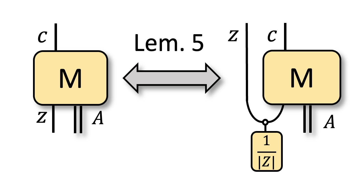
Figure 12: As an example of Lemma 5, a multi-measurement $\{\{M_{c|z}^{A}\}_{c}\}_{z}$ is nonclassical if and only if the single measurement $\{\tilde{M}_{c,z}^{A}\}_{c,z}$ obtained from flag-convexification of the multi-measurement (so that $\tilde{M}_{c,z}^{A}=\frac{1}{|Z|}M_{c|z}^{A}$) is nonclassical.

The proof follows from facts about the ontological representation of flag-convexification described in Refs. [28, 64]. Specifically, it follows from the fact that all that changes when one moves from a given process to its flag-convexified counterpart is that it is rescaled by a constant factor, and so an ontological representation of the given process can simply be rescaled by the same constant factor to give an ontological representation of the flag-convexified process.

The third lemma states that the nonclassicality of a process does not depend on whether or not one reconceptualizes its classical outputs as quantum systems that are dephased in a fixed basis.

Lemma 6.

Whether or not a process is nonclassical (in the sense of our proposal, Definition $3^{\prime}$) is independent of whether one reconceptualizes its classical outputs as dephased quantum systems.

(In the next section, we show that the analogous result is true also for classical inputs.)

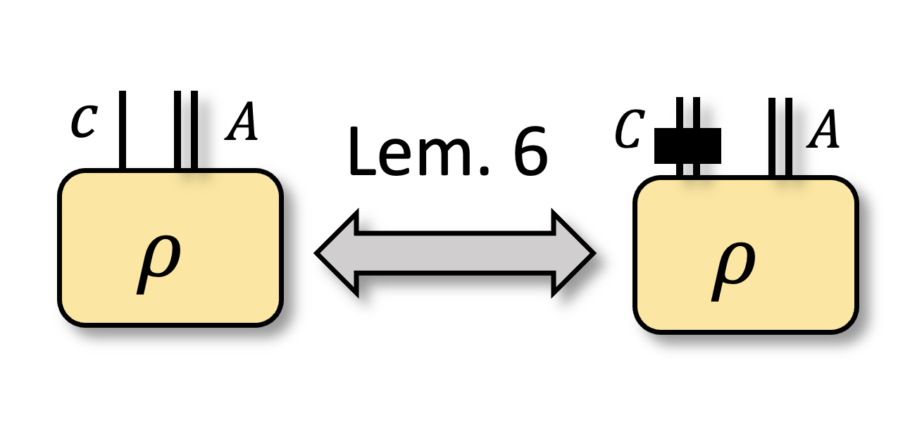
Figure 13: As an example of Lemma 6, a source $\{p(c)\rho_{c}^{A}\}$ is nonclassical if and only if the bipartite state $\tilde{\rho}^{CA}=\sum_{c}p(c)|c\rangle\langle c|^{C}\otimes\rho^{A}_{c}$ obtained by viewing its classical outcome as a dephased quantum output is nonclassical. Here, the dark square represents the fact that the system is dephased in the given basis $\{|c\rangle\}$.

This is proven in Appendix K.

Theorem 6 follows immediately by combining the three lemmas. It follows that by characterizing the nonclassicality of arbitrary multipartite states, one is in fact able to characterize the nonclassicality of arbitrary processes in quantum theory.

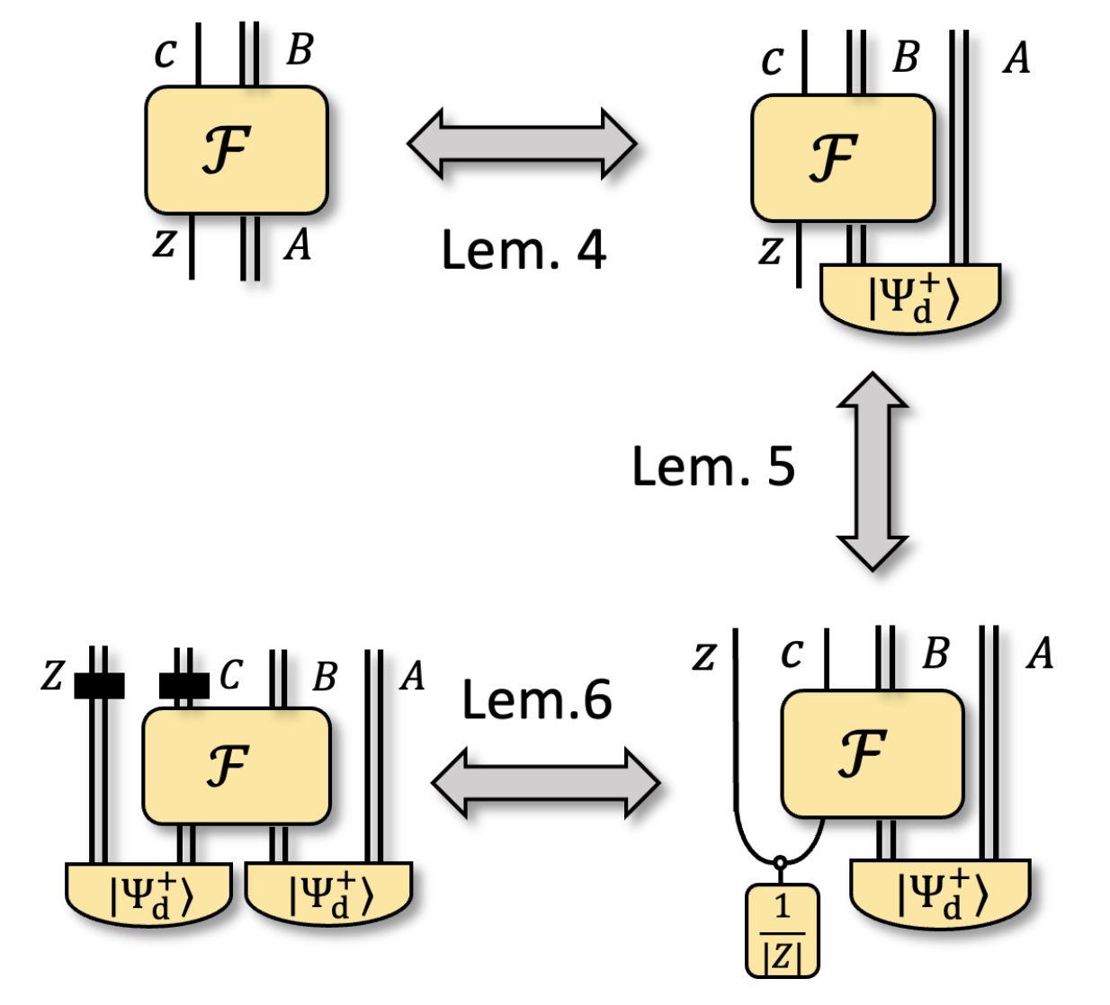
Figure 14: A multi-instrument $\{\{\mathcal{F}_{c|z}^{A\rightarrow B}\}_{c}\}_{z}$ is nonclassical if and only if the associated multipartite state $\rho^{ZCBA}=\sum_{cz}\frac{1}{|Z|}p(c|z)|z\rangle\langle z|\otimes|c\rangle\langle c|\otimes\rho_{\mathcal{F}_{c|z}}^{BA}$ is nonclassical, where $p(c|z)\rho^{BA}_{\mathcal{E}_{c|z}}=(\mathcal{F}_{c|z}^{A\rightarrow B}\otimes\mathbb{1}^{A})|\Psi^{+}\rangle\langle\Psi^{+}|^{AA}$. For the final equivalence, we note that a perfectly correlated probability distribution on a pair of classical variables $\{p(z,z^{\prime})=\frac{1}{|Z|}\delta_{z,z^{\prime}}\}$ can be reconceptualized as a dephased maximally entangled state.

The nonclassicality of multipartite states can be characterized in a manner analogous to what was done for bipartite states in Proposition 1 and Theorem 4.

Theorem 7.

A multipartite state is classical if the set of states one can steer to is classical for every possible bipartition of its subsystems (into a set being measured and a set being steered).

This is proven in Appendix M.

As argued just above, this provides a means of characterizing the nonclassicality for arbitrary processes in quantum theory.

Moreover, a multipartite state that is entangled across any partition is nonclassical. That is, Theorem 7 implies the generalization of Theorem 4 from bipartite to multipartite systems. The proof of this implication follows the same logic as the proof of the implication from Proposition 1 to Theorem 4.

In the multipartite case (just as in the bipartite case), separability is necessary but not sufficient for classicality. That is, there exist multipartite states that are not entangled across any partition and that are nonclassical. It suffices to consider multipartite generalizations of Example 5.

One can also find tripartite states that can be steered to nonclassical sets of states on any of the three parties.

Example 7.

Given a tripartite state defined as

$$\rho^{B_{1}B_{2}B_{3}} =\frac{1}{4}(|000\rangle\langle 000|+|-+1\rangle\langle-+1|$$ (52)

$$+|1-+\rangle\langle 1-+|+|+1-\rangle\langle+1-|),$$ (53)

there exist measurements on any two subsystems that steer the remaining system to a set of states that is nonclassical. In particular, if any two parties each perform the BB84 measurement, which is associated to the POVM $\{\frac{1}{2}|0\rangle\langle 0|,\frac{1}{2}|1\rangle\langle 1|,\frac{1}{2}|+\rangle\langle+|,\frac{1}{2}|-\rangle\langle-|\}$, then they steer the third party’s system to the ensemble containing the unnormalized states

$$\{\frac{3}{64}(\frac{2}{3}\rho_{x}+\frac{1}{3}\sigma_{y}),\frac{3}{64}(\frac{1}{3}\rho_{x}+\frac{2}{3}\sigma_{y})\}_{x,y}$$

$$\cup \{\frac{5}{64}(\frac{3}{5}\rho_{x}+\frac{1}{5}\mathbb{I}),\frac{5}{64}(\frac{1}{5}\rho_{x}+\frac{2}{5}\mathbb{I})\}_{x}$$

$$\cup \{\frac{5}{64}(\frac{3}{5}\sigma_{y}+\frac{1}{5}\mathbb{I}),\frac{5}{64}(\frac{1}{5}\sigma_{y}+\frac{2}{5}\mathbb{I})\}_{y},$$ (54)

where $\rho_{x}\in\{|0\rangle\langle 0|,|1\rangle\langle 1|\},\sigma_{y}\in\{|+\rangle\langle+|,|-\rangle\langle-|\}$, which can be shown to be nonclassical using the semidefinite program given in Ref. [70].

An interesting open question is whether, when assessing the nonclassicality of a multipartite state, it suffices to consider the nonclassicality of the sets of states one can steer to on each subsystem of the multipartition. We have not managed to settle this question one way or the other. If considering single-party steering possibilities does suffice, this will dramatically simplify the tractability of the task of characterizing nonclassicality of multipartite states (and hence general processes), by allowing one to reduce the problem to a linear program. If it does not, then this will constitute a new way in which the nonclassicality of a state can be judged to be genuinely multipartite [96, 3, 97, 98].

VIII Consistency under reconceptualizing settings and outcomes as dephased quantum systems

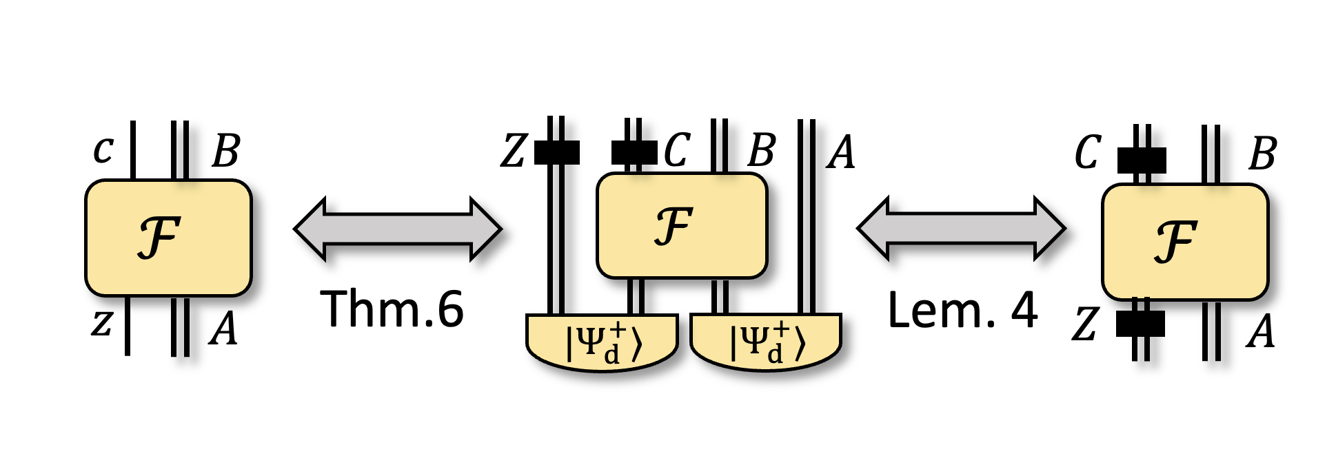
Figure 15: The proof that nonclassicality is preserved under reconceptualizing classical inputs and outputs as dephased quantum systems.

A basic consistency condition for any notion of classicality is that it should not depend on the theorist’s representational choices. In particular, it should not depend on whether one represents the classical inputs and outcomes of a given process as quantum systems that are dephased in an appropriate basis, or as classical systems. This is an instance of the principle of cut motility [99], which states that the claims made by a physical theory that purports to be universally applicable should not change when one’s experimental apparatuses are modeled explicitly within the theory.

The notion of classicality we have introduced here satisfies this principle. For classical outputs, Lemma 6 already gives the result, and we can use the three lemmas from the previous section to extend this result to classical inputs, following the logic shown in Figure 15.

Although this kind of consistency may seem quite basic, intuitive attempts to stitch together different notions of classicality in the literature can fail to be consistent in this manner, and so fail to provide a unified notion of classicality. For instance, consider sets of bipartite states, as shown in the lefthand side of Figure 16. Intuitively, one might argue that the nonclassical objects of this form are all and only those sets of states that contain at least one entangled state. In the special case where system $C$ is a classical system, this would imply that all such processes are classical. However, this would be inconsistent with the standard notion of classicality for assemblages, shown on the right-hand side of Figure 16, which states that some processes of this form (namely the steerable ones [100], or equivalently, the LOSR-nonfree ones [2, 83]) are nonclassical.

Consequently, if one cares to have a unified notion of nonclassicality for arbitrary processes, such basic consistency checks are essential.

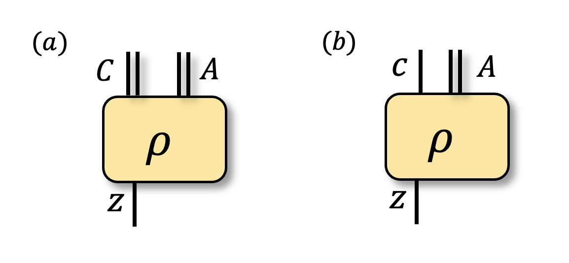
Figure 16: (a) A set of bipartite states. (b) A set of bipartite classical-quantum states (none of which can be entangled); viewed as assemblages, however, some such sets are nonclassical (in the sense that they are steerable).

Example 8.

An assemblage $\{\{p(a|x)\rho_{a|x}\}_{a}\}_{x}=\{\{\frac{1}{2}|0\rangle\langle 0|,\frac{1}{2}|1\rangle\langle 1|\},\{\frac{1}{2}|+\rangle\langle+|,\frac{1}{2}|-\rangle\langle-|\}\}$ is nonclassical in the steering scenario. If one treats the classical outcome variable as a quantum outcome, however, it corresponds to a set of separable state $\{\rho_{1},\rho_{2}\}$, where

$$\rho_{1} =|0\rangle\langle 0|\otimes|0\rangle\langle 0|+|1\rangle\langle 1|\otimes|1\rangle\langle 1|$$ (55)

$$\rho_{2} =|0\rangle\langle 0|\otimes|+\rangle\langle+|+|1\rangle\langle 1|\otimes|-\rangle\langle-|.$$ (56)

This example also corroborates our result that some separable states are nonclassical. While some readers may find themselves resisting this claim, based on intuitions stemming from the widespread view that entanglement is the fundamental notion of nonclassicality for bipartite states, it may be helpful to recognize that in the context of quantum steering, the standard view is that steerable assemblages are nonclassical—and steerable assemblages are just sets of separable quantum states (when the classical outputs are reconceptualized as dephased quantum systems).

IX Related works

Another approach to defining a classical-nonclassical divide in a manner that follows a unified principle which applies across a wide range of types of processes is the type-independent resource theory in Ref. [2, 3]. This approach defines a notion of nonclassicality of common cause which applies to processes such as multipartite states, boxes (i.e., processes with multiple classical inputs and classical outputs), assemblages, and so on. However, the classical-nonclassical divide defined by this approach is trivial for unipartite processes, and it is moreover not clear how to generalize this approach to arbitrary causal structures (although first steps were discussed in Appendix A.3 of Ref. [1].

It is nonetheless useful to contrast this approach with the one we propose here. One way to understand the relationship between the two is that classicality as defined in the LOSR approach demands that the ontological accounts of the statistics has a causal structure that mirrors that of the quantum circuit (an instance of assuming diagram-preservation), while the approach here demands in addition that the ontological representation map be linear. This stronger assumption is motivated by the principle of generalized-noncontextuality, and implies that the set of processes that is found to be nonclassical is broader than the set that is found when one does not assume linearity. For instance, there are processes on unipartite systems that are judged to be nonclassical.

Several previous works [101, 30, 102] also studied the properties of a bipartite state that are pertinent to its ability to support a proof of contextuality, in the following sense. In a steering scenario for a bipartite system $A_{1}A_{2}$, if one considers implementing any local measurement on $A_{1}$, the bipartite state on $A_{1}A_{2}$ induces a set of sources on $A_{2}$. These sources, together with an arbitrary measurement on $A_{2}$ constitutes a prepare-measure circuit, and one can ask whether the statistics of this prepare-measure circuit admit of a noncontextual ontological model. In particular, these prior works have studied the connection between these sorts of properties of a bipartite state and their entanglement properties, steering properties and nonlocal properties.

However, none of these works considered the full set of operational identities in the bipartite scenario (listed in Eq. (34)), as is essential if one wishes to define or fully characterize classicality of a bipartite state. Essentially, all these works consider the prepare-and-measure scenario induced by steering from one party to another. Consequently, they only consider the operational identities $\mathcal{O}_{\mathsf{M}_{1}\circ\mathsf{P}}$ and $\mathcal{O}_{\mathsf{M}_{2}}$ (or a subset thereof), while omitting the identities that arise when considering the preparation steered in the opposite direction, from $A_{2}$ to $A_{1}$, namely $\mathcal{O}_{\mathsf{M}_{2}\circ\mathsf{P}}$ and $\mathcal{O}_{\mathsf{M}_{1}}$.

To be more specific, the work by Tavakoli and Uola [103] considers only the operational identities in $\mathcal{O}_{\mathsf{M}_{2}}$ and a subset of the operational identities in $\mathcal{O}_{\mathsf{M}_{1}\circ\mathsf{P}}$—namely, those implied by the no-signaling principle. The results of Wright and Farkas [54] rely on a still smaller set of operational identities, including those following from no-signaling, together with a subset of the operational identities in $\mathcal{O}_{\mathsf{M}_{2}}$, specifically those arising from the normalization condition $\sum_{b}M_{b|y}=\sum_{b}M_{b|y^{\prime}}$. Plavala and Gühne [101], in comparison, do consider all operational identities in the prepare-and-measure scenario induced by steering to states on system $A_{2}$, but they do not consider all operational identities on the full bipartite scenario.

Because these earlier works impose fewer constraints on the ontological model than we do here, the results they derive do not fully characterize the classical-nonclassical divide for bipartite states according to our proposal. This is consistent with the statement of the results in those works, which makes clear that they were not claiming to capture the full constraints implied by noncontextuality. The one exception to this, however, is Theorem 2 in [30], whose statement suggests that it leverages all of the ontological constraints following from the assumption of noncontextuality in the scenario under study. However, the argument purporting to prove the theorem does not in fact take into account all such constraints. We discuss this further in Ref. [70].

X Conclusion

In this work, we introduced a notion of nonclassicality for individual quantum processes. There are many avenues for future work, including the obvious questions of finding further examples of nonclassical processes and characterizing the nonclassical processes of a given type. Another natural question would be to generalize Theorem 2 and Theorem 3 to arbitrary types of processes. Another interesting question would be to ask: given a particular nonclassical process, what are the sets of dual processes relative to which its nonclassicality can be witnessed? For any given process, there will be many such sets of dual processes, and these form a partial order under set inclusion. One could then study this partial order as a means to understand what is required to witness nonclassicality. For instance, one could seek to find the least elements in this partial order.

This work focused on the decision problem regarding the classical-nonclassical divide: assessing whether a given process is classical or nonclassical. An important open problem is that of quantifying the degree of nonclassicality according to the approach introduced here. In a companion paper [70], we give some basic tools for doing so for multi-sources and multi-measurements, based on specific measures of how robust a given process is to noise.

The most principled and informative approach to the quantification problem, however, is to pursue it within the framework of resource theories [104]. Roughly speaking, one expects that the correct choice of the divide between free and nonfree resources in the resource theory should follow from the divide between classical and nonclassical processes of that type.

One can already recognize some aspects that such a resource theory will satisfy. For example, it will not be convex, since (for example) any set of product states is classical, while some separable states are nonclassical. Similarly, the convex combination of two classical measurements can result in a nonclassical measurement. One way to understand this nonconvexity is to note that the process of mixing can introduce new operational identities, and hence new constraints on the ontological model, which in turn can activate nonclassicality.

Moreover, this work opens up new possibilities for constructing a resource theory of nonclassicality based on contextuality; for instance, it could be used to define a resource theory wherein the objects under study (the resources) are themselves simply individual quantum processes. Prior to this work, it seemed that the resources would need to be more complicated mathematical objects (such as sets of states together with sets of effects, or sets of states together with operational equivalences among these; see for example Ref. [65]).

An example of a potential application of such a resource theory is, within a Bell scenario, giving a resource-theoretic account of the simultaneous self-testing of the nonclassicality in both the bipartite state and the local measurements. This cannot be achieved in the LOSR approach to quantifying nonclassicality since although the latter can yield a resource-theoretic account of self-testing for the bipartite state, as described in Ref. [3], it cannot yield a resource-theoretic characterization of self-testing for the local measurements, since all local measurements are taken to be free in the LOSR resource theory.

In the introduction, we noted that the problem of understanding the scope of quantum-over-classical advantages for various tasks provides a motivation for understanding the classical-nonclassical divide. In recent years, it has become apparent that the framework of resource theories provides a particularly powerful perspective on this problem. Developing a unified resource theory of nonclassicality, i.e, one that applies to arbitrary types of processes (by defining the free operations in a manner that can be particularized to any type), can also be motivated by this question. By leveraging the similarity of the structure of nonclassical resources for processes of different types (for instance, multi-sources and multi-measurements), a known quantum-over-classical advantage in a task that requires nonclassicality for one particular type of process might be used to infer an advantage in a different task that requires a very different type of process.

Acknowledgements— We thank John Selby and Ana Belén Sainz for helpful discussions. YZ was supported by the Natural Sciences and Engineering Research Council of Canada (NSERC) and Canada Foundation for Innovation (CFI), YZ is grateful for the hospitality of Perimeter Institute where this work was carried out. DS, RWS, and YY were supported by Perimeter Institute for Theoretical Physics. Research at Perimeter Institute is supported in part by the Government of Canada through the Department of Innovation, Science and Economic Development and by the Province of Ontario through the Ministry of Colleges and Universities. YY was also supported by the Natural Sciences and Engineering Research Council of Canada (Grant No. RGPIN-2024-04419).

XI Appendix

Appendix A Frame representations

Consider a complex Hilbert space $\mathcal{H}$ with some finite dimension $d$. The Hermitian operators $\text{Herm}(\mathcal{H})$ on $\mathcal{H}$ form a real vector space of dimension $d^{2}$ with the Hilbert-Schmidt inner product $\langle A,B\rangle:=\textrm{Tr}[AB]$ for $A,B\in\text{Herm}(\mathcal{H})$.

Therefore, some standard vector space concepts can be brought to bear on the operator space. For instance, it is well-known that a basis of a vector space uniquely defines a dual basis in the dual vector space (i.e. the space of functionals on the vector space). We will leverage this fact, but in a slightly different form:

Lemma 7.

[19] Given any basis $\{F_{\lambda}\}_{\lambda}$ for a $d^{2}$-dimensional real vector space $\text{Herm}(\mathcal{H})$ of Hermitian operators on a Hilbert space $\mathcal{H}$, there is a unique set $\{D_{\lambda}\}_{\lambda}$ of $d^{2}$ Hermitian operators satisfying

$$\textrm{Tr}(D_{\lambda^{\prime}}F_{\lambda})=\delta_{\lambda,\lambda^{\prime}},$$ (57)

and $\{D_{\lambda}\}_{\lambda}$ also forms a basis for $\text{Herm}(\mathcal{H})$.

Proof.

Consider any basis $\{F_{\lambda}\}_{\lambda}$ of $\text{Herm}(\mathcal{H})$. It uniquely specifies a basis $\{\mathcal{D}_{\lambda}\}_{\lambda}$ of the dual vector space $\text{Herm}(\mathcal{H})^{*}$, where $\{\mathcal{D}_{\lambda}\}_{\lambda}$ are linear functionals satisfying $\mathcal{D}_{\lambda^{\prime}}(F_{\lambda})=\delta_{\lambda,\lambda^{\prime}}$. Now, in order to obtain again a set of Hermitian operators $\{D_{\lambda}\}_{\lambda}$, we use the Riesz representation theorem [105], which states that each of these functionals $\mathcal{D}_{\lambda}$ can be written as the Hilbert-Schmidt inner product with a unique Hermitian operator $D_{\lambda}$, namely $\mathcal{D}_{\lambda}(\cdot)=\textrm{Tr}{[(\cdot)D_{\lambda}]}.$ This picks out a unique basis $\{D_{\lambda}\}_{\lambda}$ which satisfies Eq. (57). ∎

More generally, one can define a frame and a dual frame as a generalization of the notion of a basis and a dual basis [106], where the vectors in both the frame and the dual are assumed to be spanning, but may or may not be linearly independent[106]. And if $\{F_{\lambda}\}_{\lambda}$ and $\{D_{\lambda}\}_{\lambda}$ are a pair of a frame and a dual frame in $\text{Herm}(\mathcal{H})$, then it follows that, for any $A\in\text{Herm}(\mathcal{H})$, one has

$$A=\sum_{\lambda}\textrm{Tr}[AD_{\lambda}]F_{\lambda}$$

$$A=\sum_{\lambda}\textrm{Tr}[AF_{\lambda}]D_{\lambda}.$$ (58)

These reconstruction equations show explicitly how every vector in the space can be expanded in terms of the spanning frame operator or spanning dual frame operators. Note that, unlike dual bases, dual frames are not necessarily unique. A detailed exploration of frames, dual frames, and their applications in quantum information science lies beyond the scope of this letter. For a more comprehensive introduction, we refer the reader to Ref. [106].

Appendix B Possibly useful results

B.1 Why the form of variability over dual processes is irrelevant

In the main text (especially Section II.3), we noted that there are many ways of ranging over all quantum states and quantum effects on a system, depending on whether the variability is introduced by classical settings or by postselecting on classical outcomes. We then claimed that the different choices one can make in this regard make no difference for qualitiative assessments of nonclassicality.

For instance, one probing scheme that allows one to range over all quantum states is to simply have a multi-state whose classical setting is a continuous variable ranging over all (normalized) quantum states. Now, it is not hard to see that if an ontological model exists for this multi-state together with certain quantum measurements, then there also exists an ontological model for any multi-source which generates the same quantum states when one conditions on its inputs and outputs. This is because a multi-source is simply a collection of (possibly subnormalized) quantum states. But the representation of a collection of states is simply the associated collection of representations of the states; moreover, by the linearity of any ontological model, one can uniquely extend the representation of the normalized states to an ontological representation of subnormalized versions of those same states.

The story is similar for measurements. An ontological model for some set of measurements constitutes a collection of representations of all of the effects appearing in those measurements. These response functions serve to define a valid and empirically adequate ontological model for any other set of measurements that contains the same set of effects. Consequently, the existence of a (linear and empirically adequate) mapping from the set of all quantum effects to their representation as response functions implies the existence of a such a mapping for any multi-measurement one could construct with those effects.

(This is another way of understanding why verdicts of nonclassicality are unchanged under flag-convexification. Whether one fixes a certain input setting value, or postselects on the corresponding flag variable taking that same value, one is simply choosing between two different physical instantiations of the same variability, so an ontological representation for one directly gives an ontological representation for the other.)

Appendix C Proof that factorizing duals are sufficient

We now prove Theorem 1, that the definitions of nonclassicality relative to duals or to factorizing duals are the same. In other words, we prove that Definition 3 is equivalent to Definition $3^{\prime}$.

In the following two subsections, we prove the result for bipartite states and for transformations, respectively. The generalization of the proof to arbitrary types of processes is straightforward.

Although the proof is somewhat long, its basic idea is simple. First, note that every quantum process with multipartite inputs and/or outputs can be written as a linear combination of processes which factorize across the inputs and outputs. From this and the assumption that an ontological model is diagram-preserving and linear, one can then uniquely extend any given ontological model defined for all product processes in quantum theory to a quasiprobabilistic representation of all processes in quantum theory, including the nonproduct ones. It remains only to show that for the relevant processes in question, this quasiprobabilistic representation is in fact a valid probabilistic representation (e.g. is positive and normalized appropriately), a fact which follows easily from frame representation theory [107].

C.1 Factorizing duals for bipartite states

We first prove the theorem for the special case where the given process is a bipartite state. That is, we prove that the definition of nonclassicality for a bipartite state is the same whether one defines it relative to global or factorizing dual processes.

Lemma 8.

The statistics generated by a bipartite state together with all bipartite effects are classical if and only if the statistics generated by it with all product effects are classical.

Proof.

The proof for the only if direction is simply that factorizing product bipartite effects are special cases of general bipartite effects. So if the statistics generated by a bipartite state with all bipartite effects are classically explainable, then those generated by that state with all product effects are classically explainable.

Now we prove the if direction. If the statistics generated by a bipartite state $\rho^{A_{1}A_{2}}$ with every product bipartite effect $M_{1}^{A_{1}}\otimes M_{2}^{A_{2}}$ are classically explainable, then from Proposition 2, the state $\rho^{A_{1}A_{2}}$ must be separable, and therefore can be decomposed as:

$$\rho^{A_{1}A_{2}}=\sum_{\lambda_{1}\lambda_{2}}p(\lambda_{1}\lambda_{2})\sigma^{A_{1}}_{\lambda_{1}}\otimes\sigma^{A_{2}}_{\lambda_{2}}$$ (59)

Moreover, for every effect $\mathbb{0}\leq M_{i}^{A_{i}}\leq\mathbb{1}_{i}$, the linearity of the ontological model together with Gleason’s theorem implies that one can write $p(M_{i}^{A_{i}}|\lambda_{i})=\textrm{Tr}{[M_{i}^{A_{i}}\sigma_{\lambda_{i}}^{B_{i}}]}$, and so the bipartite statistics can be reproduced with the ontological model

$$\textrm{Tr}[(M_{1}^{A_{1}}\otimes M_{2}^{A_{2}})\rho^{A_{1}A_{2}}]$$ (60)

$$= \sum_{\lambda_{1}\lambda_{2}}p(\lambda_{1}\lambda_{2})p(M_{1}^{A_{1}}|\lambda_{1})p(M_{2}^{A_{2}}|\lambda_{2}).$$

In quantum theory, any bipartite effect $M^{A_{1}A_{2}}\in\mathcal{L}({\mathcal{H}^{B_{1}}\otimes\mathcal{H}^{B_{2}}})$ can always be decomposed into linear combinations of product effects (see Fig. 17), as

$$M^{A_{1}A_{2}}=\sum_{k_{1},k_{2}}r_{k_{1}k_{2}}M^{A_{1}}_{k_{1}}\otimes M^{A_{2}}_{k_{2}}$$ (61)

with some real coefficients $\{r_{k_{1}k_{2}}\}_{k_{1}k_{2}}$. Consequently, we can define a unique quasiprobability representation for $M^{A_{1}A_{2}}$ as the unique linear extension of the ontological model for product states, via

$$p(M^{A_{1}A_{2}}|\lambda_{1}\lambda_{2})\coloneqq \sum_{k_{1}k_{2}}r_{k_{1}k_{2}}p(M_{1}^{A_{1}}|\lambda_{1})p(M_{2}^{A_{2}}|\lambda_{2})$$

$$= \sum_{k_{1},k_{2}}r_{k_{1}k_{2}}\textrm{Tr}[M^{A}_{k_{1}}\sigma^{A_{1}}_{\lambda_{1}}]\textrm{Tr}[M^{B}_{k_{2}}\sigma^{A_{2}}_{\lambda_{2}}]$$

$$= \textrm{Tr}[M^{A_{1}A_{2}}\sigma^{A_{1}}_{\lambda_{1}}\otimes\sigma^{A_{2}}_{\lambda_{2}}]$$ (62)

The form of Eq. (62) immediately guarantees that the representation map is linear and diagram-preserving. Furthermore, since $\sigma^{A_{1}}_{\lambda_{1}}$ and $\sigma^{A_{2}}_{\lambda_{2}}$ are valid quantum states, $p(M^{A_{1}A_{2}}|\lambda_{1}\lambda_{2})\in[0,1]$ defines a valid stochastic representation.

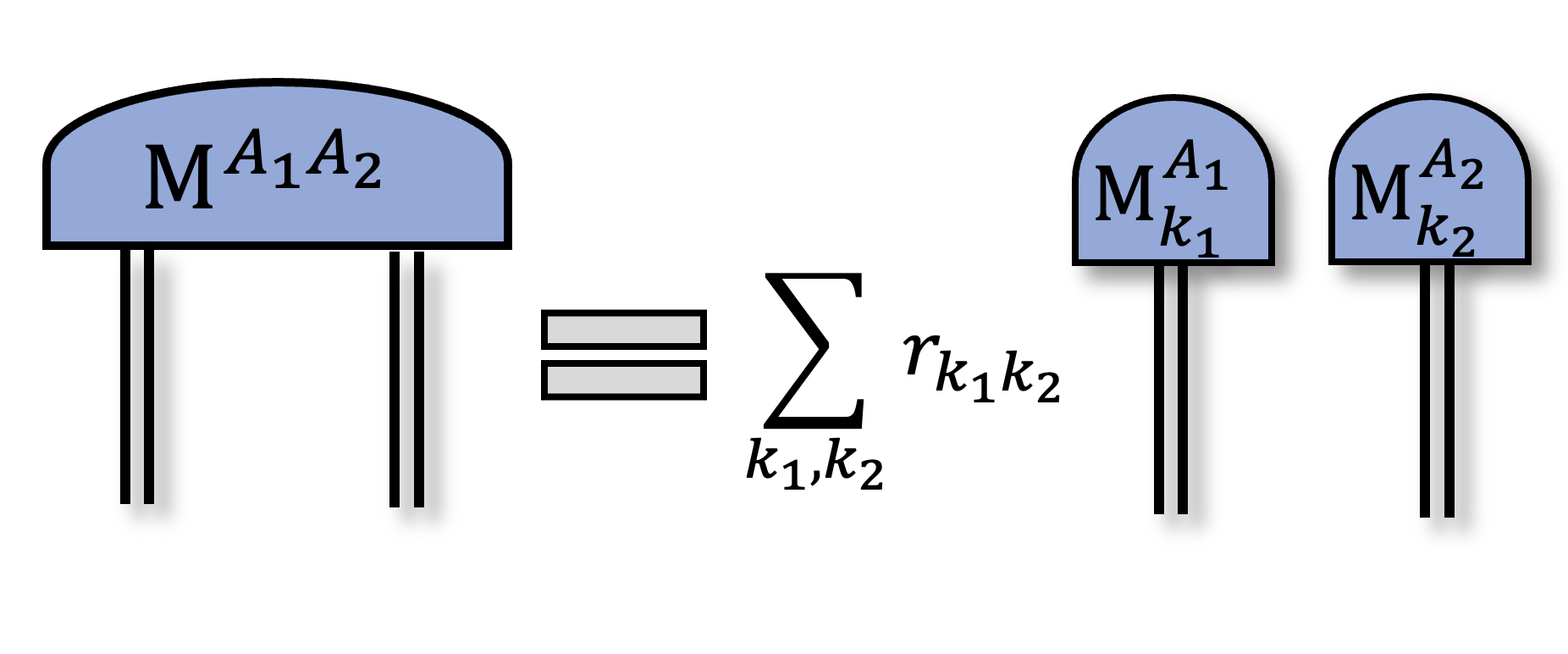
Figure 17: In quantum theory, every effect can be decomposed as a linear combination of product effects.

Finally, it is straightforward to verify that the ontological model for the given effect and state $\rho^{A_{1}A_{2}}$ reproduces the quantum statistics:

$$\sum_{\lambda_{1}\lambda_{2}}p(M^{A_{1}A_{2}}|\lambda_{1}\lambda_{2})p(\lambda_{1}\lambda_{2}|\rho^{A_{1}A_{2}})$$ (63)

$$= \sum_{k_{1}k_{2}}r_{k_{1}k_{2}}\textrm{Tr}[M^{A_{1}}_{k_{1}}\otimes M^{A_{2}}_{k_{2}}\rho^{A_{1}A_{2}}]$$ (64)

$$=\textrm{Tr}[M^{A_{1}A_{2}}\rho^{A_{1}A_{2}}].$$ (65)

Thus, $p(M^{A_{1}A_{2}}|\lambda_{1}\lambda_{2})$ gives a valid ontological representation for a generic bipartite effect $M^{A_{1}A_{2}}$ in this context, and consequently, any statistics generated by $\rho^{A_{1}A_{2}}$ with any bipartite effect are classical. ∎

C.2 Factorizing duals for transformations

Next we prove that the statistics for the set of circuits generated by contracting the transformation of interest with all dual combs are classically explainable if and only if this is the case with all factorizing dual combs.

Before proving this, we include an aside to clarify what an ontological model for a circuit including a comb looks like, since (to our knowledge) the ontological representation of quantum combs has not been explicitly studied in the literature. However, the fully compositional definitions given in Ref. [8] can be applied to this special case, resulting in the following.

We consider the specific class of combs which are dual processes for a given transformation $\cal E$ from $\mathcal{L}(\mathcal{H}^{A})$ to $\mathcal{L}(\mathcal{H}^{B})$, as shown in the top left of Figure 18. These are examples of 2-combs [78] only with a quantum output on on $\mathcal{L}(\mathcal{H}^{A})$ and takes quantum input on $\mathcal{L}(\mathcal{H}^{B})$, which will be denoted as $\mathcal{C}$.

An ontological model of this circuit associates to $\cal E$ a substochastic map $p_{\mathcal{E}}(\lambda^{\prime}|\lambda)$ and associates to each comb $\mathcal{C}$ a stochastic map $p_{\mathcal{C}}(\lambda|\lambda^{\prime})$, where moreover $p_{\mathcal{C}}(\lambda|\lambda^{\prime})=p_{\mathcal{C}}(\lambda)$. This last condition is simply the constraint that the stochastic map is nonsignaling from inputs to outputs that precede them—a fact which is an immediate consequence of the fact that the quantum comb itself satisfies this no-signaling condition. As always for an ontological model, the map from the quantum processes (in this case, from the set of combs) to their representations must be linear, and moreover the composition of the processes within quantum theory must equal the composition of their representations (so that the empirical predictions of quantum theory are reproduced). Linearity implies that the $p_{\mathcal{C}}(\lambda|\lambda^{\prime})$ obey the constraints implied by all operational identities among combs, while the latter fact implies that

$$p(\mathcal{C}\circ\mathcal{E})=\sum_{\lambda\lambda^{\prime}}p_{\mathcal{C}}(\lambda|\lambda^{\prime})p_{\mathcal{E}}(\lambda^{\prime}|\lambda).$$ (66)

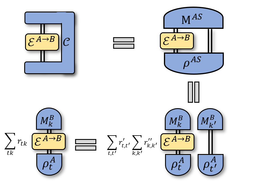
Figure 18: Global comb can be decomposed as pairs of state and effect.

We can now give the main argument.

Lemma 9.

The statistics generated by a quantum channel together with all global combs are nonclassical if and only if the statistics generated by it with some factorizing pairs of effect and state is nonclassical.

Proof.

The only if part is trivial as global comb takes factorizing pair of effect and state as special case, so let now focus on proving the if direction.

Now we prove the if direction. If the statistics generated by a quantum channel $\mathcal{E}^{A\rightarrow B}$ with every pair of state $\rho^{A}$ and effect $M^{B}$ are classically explainable, then from Proposition 4, the quantum channel $\mathcal{E}^{A\rightarrow B}$ must be entanglement-braking and thus [100] can be expressed in the Holevo form

$$\mathcal{E}^{A\rightarrow B}(\cdot)=\sum_{\lambda}\textrm{Tr}[G_{\lambda}^{A}(\cdot)]\sigma_{\lambda}^{B},$$ (67)

where the $\sigma_{\lambda}^{B}$s are density operators and $\{G_{\lambda}^{A}\}_{\lambda}$ forms a POVM. Let us define an ontological representation of the channel $\mathcal{E}^{A\rightarrow B}$ by

$$p_{\mathcal{E}}(\lambda^{\prime}|\lambda)\coloneqq\delta_{\lambda^{\prime},\lambda},$$ (68)

of the quantum effect $M^{B}$ by

$$p(M^{B}|\lambda^{\prime})\coloneqq\textrm{Tr}{[M^{B}\sigma_{\lambda^{\prime}}^{B}]},$$ (69)

and of the quantum state $\rho^{A}$ by

$$p(\lambda|\rho^{A})\coloneqq\textrm{Tr}[G^{A}_{\lambda}\rho^{A}].$$ (70)

One can check that these choices together reproduce the quantum statistics in the PTM circuit , since

$$\sum_{\lambda\lambda^{\prime}}p(M^{B}|\lambda^{\prime})p_{\mathcal{E}}(\lambda^{\prime}|\lambda)p(\lambda|\rho^{A})$$ (71)

$$= \sum_{\lambda\lambda^{\prime}}\textrm{Tr}{[M^{B}\sigma_{\lambda^{\prime}}^{B}]}\delta_{\lambda^{\prime},\lambda}\textrm{Tr}[G^{A}_{\lambda}\rho^{A}]$$

$$= \sum_{\lambda}\textrm{Tr}{[M^{B}\sigma_{\lambda}^{B}]}\textrm{Tr}[G^{A}_{\lambda}\rho^{A}]$$

$$= \textrm{Tr}\big{[}M^{B}\sum_{\lambda}\textrm{Tr}[G_{\lambda}^{A}(\rho^{A})]\sigma_{\lambda}^{B}\big{]}$$

$$= \textrm{Tr}[M^{B}\mathcal{E}^{A\rightarrow B}(\rho^{A})].$$

Now, we will use these representations to show that we can also construct an ontological representation of the global comb $\cal C$.

First, we will rewrite the global comb $\cal C$ within quantum theory as a linear combinations of states and effects as shown in Fig. 18; then, we will use the above representations of states and effects to construct a quasiprobabilistic representation of $\cal C$. Then we prove that this representation is in fact nonnegative and forms a valid ontological model. The detailed steps are as follows.

Specifically, it has been shown [78] that any global comb $\mathcal{C}$ can be decomposed as a bipartite state $\rho^{AS}$ followed by a bipartite measurement (effect) $M^{BS}$ with an identity channel acting on system $S$. That is

$$\mathcal{C}(\mathcal{E}^{A\rightarrow B}): =\textrm{Tr}[M^{BS}(\mathcal{E}^{A\rightarrow B}\otimes\mathbb{1}^{S\rightarrow S})\rho^{AS}].$$ (72)

Furthermore, any bipartite quantum state and bipartite measurement can be decomposed as

$$\rho^{AS}=\sum_{tt^{\prime}}r_{tt^{\prime}}^{\prime}\rho_{t}^{A}\otimes\rho_{t^{\prime}}^{S}$$ (73)

$$M^{BS}=\sum_{kk^{\prime}}r_{kk^{\prime}}^{{}^{\prime\prime}}M_{k}^{B}\otimes M_{k^{\prime}}^{S}$$ (74)

with some real coefficients $\{r_{tt^{\prime}}^{\prime}\}_{tt^{\prime}}$ and $\{r_{kk^{\prime}}\}_{kk^{\prime}}$. As such, the action of the global comb $\cal C$ on the channel ${\cal E}^{A\rightarrow B}$ can be further decomposed as

$$\mathcal{C}(\mathcal{E}^{A\rightarrow B})\coloneqq$$ (75)

$$\textrm{Tr}[(\sum_{kk^{\prime}}r_{kk^{\prime}}^{{}^{\prime\prime}}M_{k}^{B}\otimes M_{k^{\prime}}^{S})(\mathcal{E}^{A\rightarrow B}\otimes\mathbb{1}^{S\rightarrow S})(\sum_{tt^{\prime}}r_{tt^{\prime}}^{\prime}\rho_{t}^{A}\otimes\rho_{t^{\prime}}^{S})].$$

Defining the new real coefficients

$$r_{tk}\coloneqq\sum_{tt^{\prime}kk^{\prime}}r_{tt^{\prime}}^{\prime}r^{\prime\prime}_{kk^{\prime}}\textrm{Tr}[M_{k^{\prime}}^{S}\rho_{t^{\prime}}^{S}],$$ (76)

the expression for the comb $\cal C$ acting on $\cal E$ can be further simplified to

$$\mathcal{C}(\mathcal{E}^{A\rightarrow B})=\sum_{tk}r_{tk}\textrm{Tr}[M_{k}^{B}\mathcal{E}^{A\rightarrow B}(\rho_{t}^{A})].$$ (77)

This final decomposition of the comb $\cal C$ is shown on the bottom left diagram of Fig. 18.

Now, given our choice to represent states and effects as in Eq. 70 and Eq. 69, respectively, the unique linear and diagram-preserving representation of the comb $\mathcal{C}$ is

$$p_{\mathcal{C}}(\lambda|\lambda^{\prime})\coloneqq \sum_{tk}r_{tk}p(\lambda|\rho^{A}_{t})p(M_{k}^{B}|\lambda^{\prime})$$

$$= \sum_{tk}r_{tk}\textrm{Tr}[G_{\lambda}\rho^{A}_{t}]\textrm{Tr}[M^{B}_{k}\sigma^{B}_{\lambda^{\prime}}]$$

$$= \textrm{Tr}[G^{A}_{\lambda}\mathcal{C}(\sigma^{B}_{\lambda^{\prime}})].$$ (78)

Furthermore, since $G_{\lambda}^{B}$ and $\sigma_{\lambda^{\prime}}^{A}$ are valid effect and quantum states, $p_{\mathcal{C}}(\lambda|\lambda^{\prime})\in[0,1]$ defines a valid stochastic representation.

Finally, it is straightforward to verify that these representations reproduce the statistics:

$$\sum_{\lambda\lambda^{\prime}}p_{\mathcal{C}}(\lambda|\lambda^{\prime})p_{\mathcal{E}}(\lambda^{\prime}|\lambda)= \sum_{\lambda\lambda^{\prime}}\textrm{Tr}[G^{A}_{\lambda}\mathcal{C}(\sigma^{B}_{\lambda^{\prime}})]\delta_{\lambda^{\prime},\lambda}$$

$$= \sum_{\lambda}\textrm{Tr}[G^{A}_{\lambda}\mathcal{C}(\sigma^{B}_{\lambda})].$$ (79)

From Eq. 67, the Holevo form of the channel ${\cal E}^{A\rightarrow B}$, Eq. 79 evidently expresses the statistics of the comb acting on the channel (also see Fig. 19).

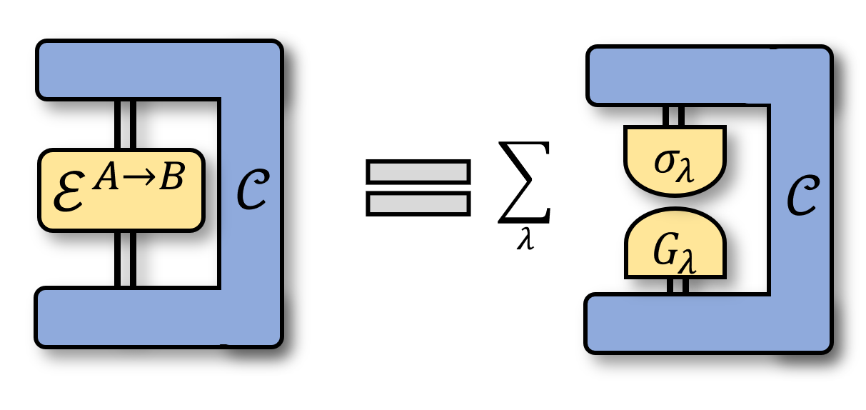
Figure 19: An entanglement breaking channel and a dual.

Thus, $p_{\mathcal{C}}(\lambda|\lambda^{\prime})$ is a valid ontological representation for a generic quantum comb $\mathcal{C}$. That is, we have seen that whenever the statistics generated by ${\cal E}^{A\rightarrow B}$ with all factorizing pairs of effect and state are classically explainable, one can write down such a representation for any global comb $\mathcal{C}$. It follows that the statistics generated by ${\cal E}^{A\rightarrow B}$ with any global comb must also be classically explainable. ∎

Appendix D Proof of Theorem 2

We now repeat and then prove Theorem 2.

Theorem 2.

A multi-source $\mathsf{P}\coloneqq\{\{p(a|x)\rho_{a|x}\}_{a}\}_{x}$ is classical (in the sense of Definition 5) if and only if it satisfies the following equivalent conditions:
(1) Each of the unnormalized states $p(a|x)\rho_{a|x}$ can be decomposed as

$${p(a|x)\rho_{a|x}=\sum_{\lambda}p(a\lambda|x)\sigma_{\lambda}\quad\forall a,x}$$ (80)

for some fixed set of normalized states $\{\sigma_{\lambda}\}_{\lambda}$ and some conditional probability distribution $p(a\lambda|x)$ satisfying

$${\sum_{ax}\alpha_{ax}p(a\lambda|x)=0\qquad\forall\{\alpha_{ax}\}_{a,x}\in\mathcal{O}_{\mathsf{P}}}$$ (81)

for all $\lambda$, where $\mathcal{O}_{\mathsf{P}}$ is defined in Eq. (13a).
(2)Each of the normalized states $\rho_{a|x}$ can be decomposed within a frame representation on span $V=\text{Span}\{\rho_{a|x}\}$ as

$$\rho_{a|x}=\sum_{\lambda}\textrm{Tr}[H_{\lambda}\rho_{a|x}]\sigma_{\lambda},\quad\forall a,x$$ (82)

where the set of frame operators is a fixed set of density operators $\{\sigma_{\lambda}\}_{\lambda}$ and the dual frame is a set of Hermitian operators $\{H_{\lambda}\}_{\lambda}$ satisfying $\sum_{\lambda}H_{\lambda}=\mathbb{1}$ and $\textrm{Tr}[H_{\lambda}\rho_{a|x}]\in[0,1]$ for all $a,x,\lambda$.

Proof.

We first prove that a multi-sourc $\{p(a|x)\rho_{ax}\}_{ax}$ being classical will imply $(2)$. From Definition 5, we know that the statistics generated by a classically explainable multi-source $\{\{p(a|x)\rho_{a|x}\}_{a}\}_{x}$ with any quantum effect can be expressed as

$$\textrm{Tr}[M\rho_{a|x}]=\sum_{\lambda}p(M|\lambda)p(\lambda|a,x)~~~\forall a,x,M\in\mathcal{M}(\mathcal{H})$$

where $\{p(\lambda|a,x)\}_{ax}$ depends linearly on $\{\rho_{a|x}\}_{ax}$ and $p(M|\lambda)$ depends linearly on all quantum effects $M\in\mathcal{M}(\mathcal{H})$. We can use the generalized Gleason’s theorem [89] to write the latter map as $p(M|\lambda)=\textrm{Tr}{[M\sigma_{\lambda}]}$ with a unique normalized density matrix $\sigma_{\lambda}$. Similarly, for any linear map from states $\{\rho_{a|x}\}_{ax}$ to real value $\{p(\lambda|a,x)\}_{ax}$, there always exists some Hermitian operator $H_{\lambda}$ such that $p(\lambda|a,x)=\textrm{Tr}[H_{\lambda}\rho_{a|x}]$. Therefore, we have, for any given $a$ and $x$,

$$\textrm{Tr}[M\rho_{a|x}] =\sum_{\lambda}\textrm{Tr}{[M\sigma_{\lambda}]}\textrm{Tr}[H_{\lambda}\rho_{a|x}]$$

$$=\textrm{Tr}\big{[}M\sum_{\lambda}\textrm{Tr}[H_{\lambda}\rho_{a|x}]\sigma_{\lambda}\big{]},\quad\forall M,$$ (83)

where $\textrm{Tr}[H_{\lambda}\rho_{a|x}]=p(\lambda|a,x)\in[0,1]$ (as $p(\lambda|a,x)\in[0,1]$) and $\sum_{\lambda}H_{\lambda}=\mathbb{1}_{V}$ (as $\sum_{\lambda}p(\lambda|a,x)=1$) for all $a,x,\lambda$. Since Eq. 83 must hold for all $M$, it follows that

$$\rho_{a|x} =\sum_{\lambda}\textrm{Tr}[H_{\lambda}\rho_{a|x}]\sigma_{\lambda}.$$ (84)

To show $(2)\rightarrow(1)$, we can simply define

$$p(\lambda|a,x)\coloneqq\textrm{Tr}[H_{\lambda}\rho_{a|x}].$$

$$\Rightarrow p(a\lambda|x)\coloneqq\textrm{Tr}[H_{\lambda}p(a|x)\rho_{a|x}]$$ (85)

where $\{p(a\lambda|x)\}_{ax}$ depends linear on $\{p(a|x)\rho_{ax}\}_{ax}$, which thus respects the operational identities $\mathcal{O}_{\mathsf{P}}$.

To show $(1)$ ensures the classicality of the multi-source $\{p(a|x)\rho_{ax}\}_{ax}$, we can define $p(M|\lambda):=\textrm{Tr}[\sigma_{\lambda}M]$ and thus:

$$\textrm{Tr}[M\rho_{a|x}]=\sum_{\lambda}\textrm{Tr}{[M\sigma_{\lambda}]}p(\lambda|a,x),\quad\forall M,a,x,$$ (86)

$$p(a|x)\textrm{Tr}[M\rho_{a|x}]=\sum_{\lambda}\textrm{Tr}{[M\sigma_{\lambda}]}p(a\lambda|x),\quad\forall M,a,x,$$

where $\{p(a\lambda|x)\}_{ax}$ respects $\mathcal{O}_{\mathsf{P}}$ and $p(M|\lambda)$ defines a stochastic map that is linear to all quantum effect $M\in\mathcal{M}(\mathcal{H})$. Thus, there exists an ontological model for the statistics generated by the multi-source with any quantum effect, meaning that $\{\{p(a|x)\rho_{a|x}\}_{a}\}_{x}$ is classically explainable. ∎

Appendix E Proof of Theorem 3

We now repeat and then prove Theorem 3.

Theorem 3.

A multi-measurement $\mathsf{M}=\{\{M_{b|y}\}_{b}\}_{y}$ is classical (in the sense of Definition 6) if and only if it satisfies the following equivalent conditions:
(1) Its effects can be decomposed as

$$M_{b|y}=\sum_{\lambda}p(b|y\lambda)G_{\lambda}\quad\forall b,y$$ (87)

where $\{G_{\lambda}\}_{\lambda}$ is a POVM and $p(b|y\lambda)$s are conditional probability distributions (i.e., $p(b|y\lambda)\in[0,1]$ and $\sum_{b}p(b|y\lambda)=1$) respecting the operational identities $\mathcal{O}_{\mathsf{M}}$ defined by the multi-measurement, i.e., for all $\lambda$,

$$\sum_{by}\beta_{by}p(b|\lambda,y)=0\qquad\forall\{\beta_{by}\}_{by}\in\mathcal{O}_{\mathsf{M}}.$$ (88)

(2) Its effects can be decomposed within a frame representation on span $V=\text{Span}\{M_{b|y}\}$ as

$$M_{b|y}=\sum_{\lambda}\textrm{Tr}[M_{b|y}F_{\lambda}]G_{\lambda}\quad\forall b,y$$ (89)

where $\{G_{\lambda}\}_{\lambda}$ is a POVM and $\{F_{\lambda}\}_{\lambda}$ is a set of Hermitian operators satisfying $\textrm{Tr}[F_{\lambda}]=1$ and $\textrm{Tr}[M_{b|y}F_{\lambda}]\in[0,1]$ for all $b,y,\lambda$.

Proof.

We first prove that a multi-measurement $\{\{M_{b|y}\}_{b}\}_{y}$ being classical will imply conditions $(2)$. From Definition 6, we know that the statistics generated by a classically explainable multi-measurement $\{\{M_{b|y}\}_{b}\}_{y}$ with all quantum states can be expressed as

$$\textrm{Tr}[M_{b|y}\rho]=\sum_{\lambda}p(b|y\lambda)p(\lambda|\rho)~~~~\forall b,y,\rho\in\mathcal{S}(\mathcal{H})$$ (90)

where $\{p(b|y\lambda)\}_{by}$ depends linearly on $\{M_{b|y}\}_{by}$ (and so respects $\mathcal{O}_{\mathsf{M}}$) and $p(\lambda|\rho)$ depends linearly on the quantum state $\rho\in\mathcal{S}(\mathcal{H})$. Using the Riesz representation theorem, we can write this latter linear map as $p(\lambda|\rho)=\textrm{Tr}{[G_{\lambda}\rho]}$ for some unique semidefinite operator $G_{\lambda}$. Furthermore, since $\sum_{\lambda}p(\lambda|\rho)=1$, we must have that $\sum G_{\lambda}=\mathbb{1}$. Thus, $\{G_{\lambda}\}_{\lambda}$ is a POVM. Similarly, we can always write $p(b|y\lambda)=\textrm{Tr}[M_{b|y}F_{\lambda}]$ for some Hermitian operator $F_{\lambda}$. Thus,

$$\textrm{Tr}[M_{b|y}\rho] =\sum_{\lambda}\textrm{Tr}[M_{b|y}F_{\lambda}]\textrm{Tr}[G_{\lambda}\rho]$$

$$=\textrm{Tr}\big{[}\sum_{\lambda}\textrm{Tr}[M_{b|y}F_{\lambda}]G_{\lambda}\rho\big{]}\quad\forall\rho\in\mathcal{S}(\mathcal{H})$$ (91)

where $\textrm{Tr}[M_{b|y}F_{\lambda}]=p(b|y\lambda)\in[0,1]$ (as $p(b|y\lambda)\in[0,1]$) and $\textrm{Tr}[F_{\lambda}]=1$ (as $\sum_{b}p(b|y\lambda)=1$) for all $b,y\lambda$. Since Eq. 91 must hold for all $\rho$, it follows that

$$M_{b|y}=\sum_{\lambda}\textrm{Tr}[M_{b|y}F_{\lambda}]G_{\lambda}.$$ (92)

To show $(2)\rightarrow(1)$, we can simply define

$$p(b|\lambda,y)\coloneqq\textrm{Tr}[M_{b|y}F_{\lambda}],$$

It follows that the $p(b|\lambda,y)$s depend linearly on $\{M_{b|y}\}_{by}$, which therefore do respect the operational identities ${\cal O}_{\mathsf{M}}$. Furthermore, since $\textrm{Tr}[M_{b|y}F_{\lambda}]\in[0,1]$ and $\sum_{b}\textrm{Tr}[M_{b|y}F_{\lambda}]=1$, we have that the $p(b|\lambda,y)$s are conditional probabilities.

To show $(1)$ ensures the classicality of the multi-measurement $\{\{M_{b|y}\}_{b}\}_{y}$, we can define $p(\lambda|\rho)\coloneqq\textrm{Tr}[G_{\lambda}\rho]$ and thus

$$\textrm{Tr}[M_{b|y}\rho]=\sum_{\lambda}p(b|y\lambda)\textrm{Tr}{[G_{\lambda}\rho]},\quad\forall b,y,\rho\in\mathcal{S}(\mathcal{H}),$$ (93)

where $\{p(b|y\lambda)\}_{by}$ respects $\mathcal{O}_{\mathsf{M}}$ by definition, and $p(\lambda|\rho)$ defines a stochastic map that is linear on all quantum states $\rho$. Thus there exists an ontological model for the statistics generated by the multi-measurement with any quantum state, meaning that $\{\{M_{b|y}\}_{b}\}_{y}$ is classically explainable. ∎

Appendix F Proof of Corollary 1

We now repeat and then prove Corollary 1.

Corollary 1.

Any set of quantum states that fits inside a simplex within the quantum state space is classically explainable.

Proof.

Denote the vertices of the simplex of quantum states by $\{\sigma_{\lambda}\}_{\lambda}$. As each element of the multi-state $\{\rho_{\cdot|x}\}_{x}$ are in the convex hull of the $\{\sigma_{\lambda}\}_{\lambda}$, it follows that the span of the former is contained in the span of the latter. Thus, $\{\sigma_{\lambda}\}_{\lambda}$ forms a basis for the span of the $\{\rho_{\cdot|x}\}$, and so there must exist a dual basis $\{H_{\lambda}\}_{\lambda}$ such that (recalling Eq. (58))

$$\rho_{\cdot|x}=\sum_{\lambda}\textrm{Tr}[H_{\lambda}\rho]\sigma_{\lambda}.$$ (94)

Thus, we can simply define

$$p(\lambda|x):= \textrm{Tr}[H_{\lambda}\rho_{\cdot|x}],$$ (95)

which is a linear function of the density matrix, and so must satisfy all the operational identities $\mathcal{O}_{\mathsf{P}}$ defined by $\{\rho_{\cdot|x}\}_{x}$. This has the form of a classically explainable set of states given in condition 2 of Theorem 2. ∎

Appendix G Proof of Corollary 2

Corollary 2.

A set of distinct pure states on a single system is classically explainable if and only if they are linearly independent.

Proof.

The proof for the if direction follows directly from Lemma 2. The proof for the only if direction can be shown by contradiction. Suppose the states in the multi-state $\{\rho_{\cdot|x}\}_{x}$ are linearly dependent, then we must have at least one equation of the following form

$$\sum_{x}\alpha_{x}\rho_{\cdot|x}=0,$$ (96)

where $\alpha_{x}\neq 0$. If the set is classically explainable, then there exists a set $\{\sigma_{\lambda}\}_{\lambda}$ of states such that $\rho_{\cdot|x}$ can be expressed as a convex mixture of the form $\rho_{\cdot|x}=\sum_{\lambda}p(\lambda|x)\sigma_{\lambda}$ where

$$\sum_{x}\alpha_{x}p(\lambda|x)=0.$$ (97)

However, since the $\rho_{\cdot|x}$s are pure states, the convex mixture must be trivial, i.e., $p(\lambda|x)=\delta_{\lambda x}$ and $\sigma_{x}=\rho_{\cdot|x}$. Then, Eq. 97 reduces to

$$\sum_{x}\alpha_{x}\delta_{\lambda x}=0,$$ (98)

implying that $\alpha_{x}=0$ for all $x$, contradicting our earlier assumption. Hence $\{\rho_{\cdot|x}\}_{x}$ must be a linear independent set. ∎

Appendix H Proof of Proposition 1

We now repeat and then prove Proposition 1.

Proposition 1.

Any circuit with local measurements on a bipartite state (as depicted in Fig. 8(a)) is classically explainable only if the two prepare-measure circuits it induces by boxing to obtain a steering scenario (in one or the other direction, as in Fig. 8(b)) are classically explainable.

Proof.

If the statistics generated by a bipartite state $\rho^{A_{1}A_{2}}$ with any multi-measurements $\{\{M_{b_{1}|y_{1}}\}_{b_{1}}\}_{y_{1}}$ and $\{\{M_{b_{2}|y_{2}}\}_{b_{2}}\}_{y_{2}}$ are classically explainable, then they can be expressed as

$$p(b_{1}b_{2}|y_{1}y_{2})=\sum_{\lambda_{1}\lambda_{2}}p(\lambda_{1}\lambda_{2})p(b_{1}|y_{1}\lambda_{1})p(b_{2}|y_{2}\lambda_{2}),$$ (99)

where $p(b_{1}|y_{1}\lambda_{1})$ respects $\mathcal{O}_{\mathsf{M}_{1}}$, where $p(b_{2}|y_{2}\lambda_{2})$ respects $\mathcal{O}_{\mathsf{M}_{2}}$, where the composite $\sum_{\lambda_{1}}p(b_{1}|y_{1}\lambda_{1})p(\lambda_{1}\lambda_{2})$ respects $\mathcal{O}_{\mathsf{M}_{1}\circ\mathsf{P}}$, and where the composite $\sum_{\lambda_{2}}p(b_{2}|y_{2}\lambda_{2})p(\lambda_{1}\lambda_{2})$ respects $\mathcal{O}_{\mathsf{M}_{2}\circ\mathsf{P}}$.

The fact that $\lambda_{1}$ screens-off the dependence of $b_{1}$ to $\lambda_{2}$ in the bipartite circuit allows us to define

$$p(b_{1}\lambda_{2}|y_{1})\coloneqq\sum_{\lambda_{1}}p(b_{1}|y_{1}\lambda_{1})p(\lambda_{1}\lambda_{2}),$$ (100)

we thus have that

$$p(b_{1}b_{2}|y_{1}y_{2})=\sum_{\lambda_{2}}p(b_{2}|y_{2}\lambda_{2})p(b_{1}\lambda_{2}|y_{1}),$$ (101)

which recovers the prepare-measure statistics with (1) preparation with states on $\mathcal{H}^{B_{2}}$ obtained from applying $\{\{M_{b_{1}|y_{1}}\}_{b_{1}}\}_{y_{1}}$ on $\mathcal{H}^{B_{1}}$ to the bipartite state $\rho^{A_{1}A_{2}}$, i.e, the set $\{\{p(b_{1}|y_{1})\rho_{b_{1}|y_{1}}\}_{b_{1}}\}_{y_{1}}$ with

$$p(b_{1}|y_{1})\rho_{b_{1}|y_{1}}=\textrm{Tr}_{A_{1}}[(M_{b_{1}|y_{1}}^{B_{1}}\otimes\mathbb{1}^{B_{2}})\rho^{A_{1}A_{2}}],$$

and (2) the measurement is $\{\{M_{b_{2}|y_{2}}\}_{b_{2}}\}_{y_{2}}$ on $\mathcal{H}^{B_{2}}$. Evidently, $p(b_{1}\lambda_{2}|y_{1})$ respect the operational identities for the preparations, which is simply $\mathcal{O}_{\mathsf{M}_{1}\circ\mathsf{P}}$, and $p(b_{2}|y_{2}\lambda_{2})$ respects the operational identities among the measurements $\mathcal{O}_{\mathsf{M}_{2}}$. Thus, such prepare-measure statistics are classically explainable. Following the analogous arguments, we know that the prepare-measure statistics where the preparation is on ${\cal H}^{B_{1}}$ must also be classically explainable. ∎

Appendix I Proof of Proposition 3

We now repeat and then prove Proposition 3.

Proposition 3.

Any PTM circuit (as depicted in Fig. 10(a)) is classically explainable only if the two prepare-measure circuits it induces by boxing the transformations with states or with effects, as in Fig. 10(b), are classically explainable.

Proof.

The proof is similar to Proposition 1. If the quantum statistics in the PTM circuit admits of an ontological model with stochastic process satisfying all four operational identities in Eqs. (47)-(48), the ontological models for the statistics of the two prepare-measure circuits induced by boxing the transformations with the states or with the effects follow immediately. ∎

Appendix J Proof of Proposition 4

We now repeat and then prove Proposition 4.

Proposition 4.

A non-entanglement-breaking quantum channel $\mathcal{E}$ is nonclassical.

This follows immediately from Proposition 2 together with Lemma 4. Nevertheless, we will provide another simple proof here.

Proof.

Assume $\mathcal{E}$ is classically explainable per Definition 7 for any effect $M$ and any quantum state $\rho$. Then, we have

$$\textrm{Tr}[M\mathcal{E}(\rho)] =\sum_{\lambda\lambda^{\prime}}p(M|\lambda^{\prime})p(\lambda^{\prime}|\lambda)p(\lambda|\rho)$$

$$=\sum_{\lambda}p(M|\lambda)p(\lambda|\rho),$$ (102)

where the last equality holds since the causal structure of the prepare-transform-measure circuit demands that $p(M|\lambda^{\prime},\lambda)=p(M|\lambda^{\prime})$ (as $\lambda^{\prime}$ screens-off the dependence of $M$ on $\lambda$ under the diagram preservation assumption).

Since both $p(M|\lambda)$ and $p(\lambda|\rho)$ depend linearly on all quantum effects $M$ and all quantum states $\rho$, respectively, from generalized Gleason’s theorem (and the inverse version), there exists a unique POVM $\{G_{\lambda}\}_{\lambda}$ such that $p(\lambda|\rho)=\textrm{Tr}[\rho G_{\lambda}]$ and there exists a unique density operator such that $p(M|\lambda)=\textrm{Tr}[M\sigma_{\lambda}]$. Therefore:

$$\textrm{Tr}[M\mathcal{E}(\rho)]= \sum_{\lambda}\textrm{Tr}[G_{\lambda}\rho]\textrm{Tr}[M\sigma_{\lambda}]$$

$$= \textrm{Tr}\big{[}M\sum_{\lambda}\textrm{Tr}[G_{\lambda}\rho]\sigma_{\lambda}\big{]}~~~\forall\rho,M.$$ (103)

Since this holds for all quantum effects $M$, we have

$$\mathcal{E}(\rho)=\sum_{\lambda}\textrm{Tr}[G_{\lambda}\rho]\sigma_{\lambda}~~~\forall\rho$$ (104)

meaning that $\mathcal{E}$ can be expressed in the Holevo form and thus must be entanglement breaking [100]. ∎

Appendix K Proof of Lemma 4

We now repeat and then prove Lemma 4.

Lemma 4.

The Choi state isomorphic to a given process is nonclassical if and only if the process itself is nonclassical.

Proof.

We prove this explicitly for a quantum channel; the proof for more general processes follows the same logic.

Given any quantum channel $\mathcal{E}^{A\rightarrow B}$, one can define its generalized Choi operator, which is a bipartite quantum state $\rho^{BA}_{\mathcal{E}}\in\mathcal{S}(\mathcal{H}^{B}\otimes\mathcal{H}^{A})$:

$$\rho^{BA}_{\mathcal{E}}=(\mathcal{E}^{A\rightarrow B}\otimes\mathbb{1}^{A})|\Psi^{+}\rangle\langle\Psi^{+}|^{AA}$$ (105)

where $|\Psi^{+}\rangle^{{A}A}=\sum_{k}\frac{1}{\sqrt{d}}|k\rangle^{A}|k\rangle^{A}$ for some orthonormal basis $\{|k\rangle^{A}\}_{k}$ on a $d$-dimensional Hilbert space $\mathcal{H}^{A}$.

The channel is classical if and only if the prepare-transform-measure circuit shown in Figure 20(a) can be mapped to an ontological representation in a linear and diagram-preserving way. The Choi operator for the channel is classical if and only if the bipartite prepare-measure circuit shown in Figure 20(b) can be mapped to an ontological representation in a linear and diagram-preserving way. We wish to show that classicality of one implies classicality of the other, and we do so by showing that if an ontological model exists for one of these scenarios, then an ontological model exists for the other.

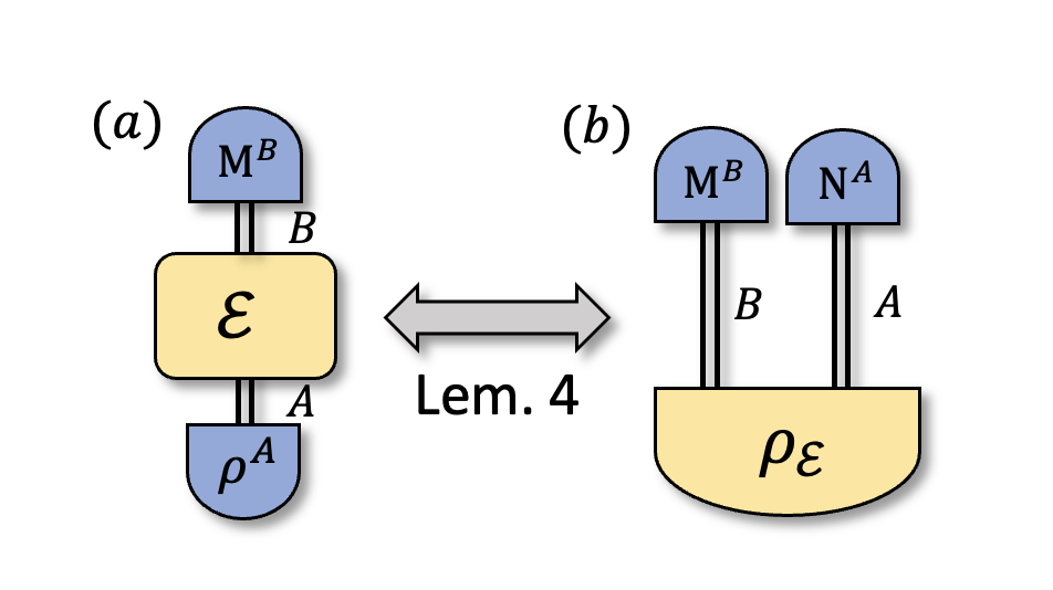
Figure 20: (a) A prepare-transform-measure circuit relevant for the proof. (b) The associated prepare-measure circuit on a bipartite system with local measurements, where $\rho^{AB}_{\mathcal{E}}$ is the Choi state associated with $\mathcal{E}$.

Imagine that the channel is classical, so that there exists an ontological model for all circuits of the form in Figure 20(a), as one varies over all quantum states and effects. Denote the representations in this ontological model by

$$M^{B}\rightarrow p(M^{B}|\lambda^{\prime})$$

$$\mathcal{E}\rightarrow p_{\mathcal{E}}(\lambda^{\prime}|\lambda)$$

$$\rho^{A}\rightarrow p(\lambda|\rho^{A}).$$

We can use this model to explicitly construct an ontological model for the circuit in Figure 20(b), as follows. First, we note that we can expand the effect $N^{A}$ in Figure 20(b) in terms of a linear sum of the density matrices $\rho_{e}^{A}=|e\rangle\langle e|^{A}$ that are projectors onto its eigenbasis $\{|e\rangle^{A}\}$ on $\mathcal{H}^{A}$, as $N^{A}=\sum_{e}r_{e}\rho^{A}_{e}$ with $r_{e}\in[0,1]$, and that we can compute the ontological representation of the maximally mixed state in the given model: $p(\lambda|\frac{\mathbb{1}^{A}}{d})=\frac{1}{d}\sum_{e}p(\lambda|\rho_{e}^{A})=\frac{1}{d}\sum_{e}p(\lambda|[\rho_{e}^{A}]^{T})$. Then, define the new ontological model by

$$M^{B} \rightarrow p(M^{B}|\lambda^{\prime})$$

$$\rho_{\mathcal{E}}^{BA} \rightarrow p(\lambda^{\prime}\lambda)=p_{\mathcal{E}}(\lambda^{\prime}|\lambda)p(\lambda|\frac{\mathbb{1}^{A}}{d})$$

$$N^{A}=\sum_{e}r_{e}\rho_{e}^{A} \rightarrow p(N^{A}|\lambda):=\frac{\sum_{e}r_{e}p(\lambda|[\rho_{e}^{A}]^{T})}{\sum_{e}p(\lambda|[\rho_{e}^{A}]^{T})}$$

$$\quad\quad\quad\quad\quad~=\frac{\sum_{e}r_{e}p(\lambda|[\rho_{e}^{A}]^{T})}{dp(\lambda|\frac{\mathbb{1}^{A}}{d})},$$ (106)

where the transpose $[\cdot]^{T}$ is defined on the basis where $|\Psi^{+}\rangle=\frac{1}{\sqrt{d}}\sum|ii\rangle$ was defined. One can directly observe that these choices are substochastic processes of the appropriate form. In addition, they reproduce the quantum predictions for the circuit, since

$$\textrm{Tr}[(M^{B}\otimes N^{A})\rho^{BA}_{\mathcal{E}}]$$ (107a)

$$= \textrm{Tr}[(M^{B}\otimes\sum_{e}r_{e}\rho^{A}_{e})\rho^{BA}_{\mathcal{E}}]$$ (107b)

$$= \textrm{Tr}[M^{B}\mathcal{E}(\sum_{e}\frac{r_{e}}{d}[\rho_{e}^{A}]^{T})]$$ (107c)

$$= \sum_{{\lambda},{\lambda}^{\prime}}p(M^{B}|\lambda^{\prime})p_{\mathcal{E}}(\lambda^{\prime}|\lambda)\sum_{e}\frac{r_{e}}{d}p(\lambda|[\rho_{e}^{A}]^{T})$$ (107d)

$$= \sum_{{\lambda},{\lambda^{\prime}}}p(M^{B}|\lambda^{\prime})p_{\mathcal{E}}(\lambda^{\prime}|\lambda)p(N^{A}|\lambda)p(\lambda|\frac{\mathbb{1}^{A}}{d})$$ (107e)

$$= \sum_{{\lambda},{\lambda^{\prime}}}p(M^{B}\lambda^{\prime})p_{\mathcal{E}}^{BA}(\lambda^{\prime}\lambda)p(N^{A}|\lambda),$$ (107f)

where we expand $N^{A}$ in its eigenbasis in the first equality, and where we utilize the Choi-isomorphism in Eq. (107b) in the second equality, the ontological representations for $M^{B}$, $\cal E$ and $\rho^{A}_{e}$ in Eq. (107c) in the third equality, and the definition of $p(N^{A}|\lambda)$in Eq. (107e).

Finally, we must check that the ontological representation constructed above is linear on all types of processes in the given circuit.

Since there is only a single bipartite state to be represented, the associated linearity condition is trivial. The representation $p(M^{B}|\lambda)$ of an arbitrary effect $M^{B}$ is trivially linear on the effect space, since the original model was given by a linear representation.

Showing that the representation of $N^{A}$ is linear on the space of effects is slightly more involved. By the Reisz representation theorem, we can always find a set of Hermitian operators $\{H_{\lambda}\}_{\lambda}$ such that the representation of states on $A$ in the original scenario can be written as $p(\lambda|\rho^{A})=\textrm{Tr}[H_{\lambda}\rho^{A}]$. Therefore, we can write the ontological representation for $N^{A}$ in the new scenario as

$$p(N^{A}|\lambda) =\frac{\sum_{e}r_{e}p(\lambda|[\rho_{e}^{A}]^{T})}{dp(\lambda|\frac{\mathbb{1}^{A}}{d})}$$

$$=\frac{1}{dp(\lambda|\frac{\mathbb{1}^{A}}{d})}\textrm{Tr}\left[\sum_{e}r_{e}[\rho_{e}^{A}]^{T}H_{\lambda}^{A}\right]$$

$$=\frac{1}{dp(\lambda|\frac{\mathbb{1}^{A}}{d})}\textrm{Tr}\left[[N^{A}]^{T}H_{\lambda}^{A}\right]$$

$$=\frac{1}{dp(\lambda|\frac{\mathbb{1}^{A}}{d})}\textrm{Tr}\left[N^{A}[H_{\lambda}^{A}]^{T}\right],$$ (108)

which is evidently linear in $N^{A}$.

Finally, we need to show that the representations of the composite processes (given by boxing one or the other effect with the bipartite state) are also linear.

The representation of the composite process $\mathcal{E}(\rho^{A})$ in the original scenario is given by $\sum_{\lambda}p_{\mathcal{E}}(\lambda^{\prime}|\lambda)p(\lambda|\rho^{A})$, and one can similarly always write this in terms of a set of Hermitian operators $\{H_{\lambda^{\prime}}^{B}\}$ such that $\sum_{\lambda}p_{\mathcal{E}}(\lambda^{\prime}|\lambda)p(\lambda|\rho^{A})=\textrm{Tr}[H_{\lambda^{\prime}}^{B}\mathcal{E}(\rho^{A})]$. Therefore, we can write the ontological representation for $\textrm{Tr}_{A}[(\mathbb{1}^{B}\otimes N^{A})\rho_{\mathcal{E}}^{BA}]$ in the new scenario as

$$\sum_{\lambda}p({\lambda}^{\prime}{\lambda})p(N^{A}|\lambda)= \sum_{\lambda}p_{\mathcal{E}}({\lambda}^{\prime}|{\lambda})p(\lambda|\frac{\mathbb{1}^{A}}{d})p(N^{A}|\lambda)$$

$$=\sum_{e}\frac{r_{e}}{d}\sum_{\lambda}p_{\mathcal{E}}({\lambda}^{\prime}|{\lambda})p(\lambda|[\rho_{e}^{A}]^{T})$$

$$=\sum_{e}\frac{r_{e}}{d}\textrm{Tr}[H_{\lambda^{\prime}}^{B}\mathcal{E}([\rho_{e}^{A}]^{T})]$$

$$=\sum_{e}{r_{e}}\textrm{Tr}[H_{\lambda^{\prime}}^{B}\otimes\rho_{e}^{A}\rho_{\mathcal{E}}^{BA}]$$

$$=\textrm{Tr}[H_{\lambda^{\prime}}^{B}\otimes N^{A}\rho_{\mathcal{E}}^{BA}],$$ (109)

which is evidently linear in $\textrm{Tr}_{A}[(\mathbb{1}^{B}\otimes N^{A})\rho_{\mathcal{E}}^{BA}]$.

Lastly, the representation of the composite process $\mathcal{E}^{\dagger}(M^{B})$ in the original PTM circuit is given by $\sum_{\lambda^{\prime}}p_{\mathcal{E}}(\lambda^{\prime}|\lambda)p(M^{B}|\lambda^{\prime})$, and we can always find a set $\{F^{A}_{\lambda}\}_{\lambda}$ of Hermitian operators such that $\sum_{\lambda^{\prime}}p_{\mathcal{E}}(\lambda^{\prime}|\lambda)p(M^{B}|\lambda^{\prime})=\textrm{Tr}[F^{A}_{\lambda}\mathcal{E}^{\dagger}(M^{B})]$. Therefore, can write the ontological representation for $\textrm{Tr}_{B}[(M^{B}\otimes\mathbb{1}^{A})\rho^{BA}_{\mathcal{E}}]$ as:

$$\sum_{\lambda^{\prime}}p(\lambda^{\prime}\lambda)p(M^{B}|\lambda^{\prime}) =\sum_{\lambda^{\prime}}p_{\mathcal{E}}({\lambda}^{\prime}|{\lambda})p(M^{B}|\lambda^{\prime})p(\lambda|\frac{\mathbb{1}}{d})$$

$$=\textrm{Tr}[F^{A}_{\lambda}\mathcal{E}^{\dagger}(M^{B})]p(\lambda|\frac{\mathbb{1}}{d})$$

$$=\textrm{Tr}[[F^{A}_{\lambda}]^{T}\mathcal{E}^{\dagger}([M^{B}]^{T})]p(\lambda|\frac{\mathbb{1}}{d})$$

$$=\textrm{Tr}[M^{B}\otimes[F^{A}_{\lambda}]^{T}\rho_{\mathcal{E}}^{BA}]dp(\lambda|\frac{\mathbb{1}}{d})$$ (110)

which is evidently linear to $\textrm{Tr}_{B}[(M^{B}\otimes\mathbb{1}^{A})\rho^{BA}_{\mathcal{E}}]$

The reverse argument is similar, so we only sketch it, focusing on the parts of the proof that are disanalogous. If a bipartite Choi state $\rho_{\mathcal{E}}^{BA}$ is classical, there exists an ontological model of the form

$$M^{B}\rightarrow p(M^{B}|\lambda^{\prime})$$

$$\mathcal{E}\rightarrow p(\lambda^{\prime}\lambda)$$

$$N^{A}\rightarrow p(N^{A}|\lambda^{\prime}).$$

We can use this model to explicitly construct an ontological model for the circuit in Figure 20(a), as follows:

$$M^{B} \rightarrow p(M^{B}|\lambda^{\prime})$$

$$\mathcal{E} \rightarrow p_{\mathcal{E}}(\lambda^{\prime}|\lambda):=\frac{p(\lambda^{\prime}\lambda)}{p(\lambda|\frac{\mathbb{1}^{A}}{d})}$$

$$\rho^{A}=\sum_{e}p_{e}N_{e}^{A} \rightarrow p(\lambda|\rho^{A}):=\sum_{e}dp_{e}p([N_{e}^{A}]^{T}|\lambda)p(\lambda|\frac{\mathbb{1}^{A}}{d})$$

where $\rho^{A}$ is expanded in its eigenbasis $\rho^{A}=\sum p_{e}N_{e}^{A}$, with $N_{e}^{A}=|e\rangle\langle e|$ and $\sum_{e}p_{e}=1$, and where $p(\lambda|\frac{\mathbb{1}}{d}):=\sum_{\lambda^{\prime}}p(\lambda^{\prime}\lambda)$ (this last notation is appropriate since the fact that the marginal of a Choi state on system $A$ is the maximally mixed state, and this is simply the representation of that.). The transpose $[\cdot]^{T}$ is defined on the basis where $|\Psi^{+}\rangle=\frac{1}{\sqrt{d}}\sum|ii\rangle$ was defined.

To see that $p(\lambda|\rho^{A})$ is a valid probability distribution, observe that $p(\lambda|\rho^{A})\geq 0$ and

$$\sum_{\lambda}p(\lambda|\rho^{A}) =\sum_{e}dp_{e}\sum_{\lambda}p([N_{e}^{A}]^{T}|\lambda)p(\lambda|\frac{\mathbb{1}}{d})$$

$$=\sum_{e}dp_{e}\frac{1}{d}=1,$$

where we used the fact that

$$\sum_{\lambda}p([N_{e}^{A}]^{T}|\lambda)p(\lambda|\frac{\mathbb{1}^{A}}{d})=\textrm{Tr}[[N_{e}^{A}]^{T}\frac{\mathbb{1}^{A}}{d}]=\frac{1}{d},$$

for rank-1 effect. The remaining processes can be shown directly to have the appropriate substochastic forms.

The quantum predictions are reproduced by this model, since

$$\textrm{Tr}[M^{B}\mathcal{E}(\rho^{A}))]$$ (111a)

$$= \textrm{Tr}[M^{B}\mathcal{E}(\sum_{e}p_{e}N_{e}^{A}))]$$ (111b)

$$= d\textrm{Tr}[(M^{B}\otimes\sum_{e}p_{e}[N_{e}^{A}]^{T})\rho^{BA}_{\mathcal{E}}]$$ (111c)

$$= \sum_{{\lambda},{\lambda^{\prime}}}p(M^{B}|\lambda^{\prime})p({\lambda}^{\prime}{\lambda})\sum_{e}dp_{e}p([N_{e}^{A}]^{T}|\lambda)$$ (111d)

$$= \sum_{{\lambda},{\lambda^{\prime}}}p(M^{B}|\lambda^{\prime})p({\lambda}^{\prime}|{\lambda})\sum_{e}dp_{e}p([N_{e}^{A}]^{T}|\lambda)p(\lambda|\frac{\mathbb{1}^{A}}{d})$$ (111e)

$$= \sum_{{\lambda},{\lambda^{\prime}}}p(M^{B}|\lambda^{\prime})p(\lambda^{\prime}|\lambda)p(\lambda|\rho^{A}).$$ (111f)

Finally, following arguments analogous to those in the first half of the proof, one can verify that the ontological representations for all the processes in the circuit are given by linear maps. Thus, the quantum channel corresponding to the bipartite Choi-state is also classical. ∎

Appendix L Proof of Lemma 6

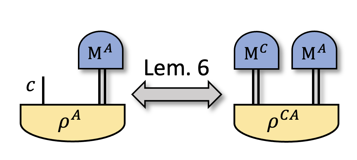
Figure 21: Connecting circuit in a prepare-measure scenario for a source, and a circuit in a prepare-measure scenario on a bipartite system with local measurements

We now prove Lemma 6.

Lemma 6.

Whether or not a process is nonclassical is independent of whether one reconceptualizes its classical outputs as dephased quantum systems.

Proof.

We prove the claim for a source $\{p(c)\rho_{c}^{A}\}$, which can be viewed as a bipartite state

$$\rho^{CA}:=\sum_{c}p(c)|c\rangle\langle c|^{C}\otimes\rho_{c}^{A}$$ (112)

when the classical output is reconceptualized as the dephased quantum system $C$. The generalization to arbitrary quantum processes follows.

For one direction, if the bipartite state is classical, following Theorem 4, it already implies that any preparation that can be made from it by local measurements must also be classical. In particular, the source $\{p(c)\rho^{A}_{c}\}$ can be generated from this bipartite state by measuring $\{M_{c}=|c\rangle\langle c|^{C}\}$ on $\sum_{c}p(c)|c\rangle\langle c|^{C}\otimes\rho_{c}^{A}$, and must be classical.

For the other direction, if the source $\{p(c)\rho_{c}^{A}\}$ is classical, according to Theorem 2, there exists a decomposition of it with

$$\rho^{A}_{c}=\sum_{\lambda}\textrm{Tr}[H^{A}_{\lambda}\rho^{A}_{c}]\sigma^{A}_{\lambda}$$ (113)

where $\sigma^{A}_{\lambda}$ are quantum states, and $\{H^{A}_{\lambda}\}$ is a set of Hermition operators with $\sum_{\lambda}H_{\lambda}^{A}=\mathbb{1}^{A}$, and $\textrm{Tr}[H^{A}_{\lambda}\rho^{A}_{c}]\geq 0$ for all $\lambda,a$.

Then, one can show that all the statistics generated by the bipartite state $\rho^{CA}$ together with any local effects $M^{C}\otimes M^{A}$ can be reproduced by the following ontological model. One takes the ontic states to be $c\times\lambda\in\Lambda_{C}\times\Lambda$, and defines the ontological representation for each process and each contracted process by

$$p(M^{C}|c) :=\textrm{Tr}[|c\rangle\langle c|^{C}M^{C}]$$

$$p(M^{A}|\lambda) :=\textrm{Tr}[\sigma_{\lambda}^{A}M^{A}]$$

$$p(c\lambda) :=\textrm{Tr}[|c\rangle\langle c|^{C}\otimes H^{A}_{\lambda}\rho^{CA}].$$

Clearly, the ontological representation of each effect is given by a linear function on the effect space; moreover, one can check that these processes are valid substochastic processes.

Finally, we must check that the ontological representation of the composite process $\textrm{Tr}_{C}[M^{C}\otimes\mathbb{1}^{A}\rho^{CA}]$ is also given by a linear function. This can be seen because it is given by

$$\sum_{c}p(c\lambda)p(M^{C}|c) =\sum_{c}\textrm{Tr}[|c\rangle\langle c|^{C}\otimes H^{A}_{\lambda}\rho^{CA}]\textrm{Tr}[|c\rangle\langle c|^{C}M^{C}]$$

$$=\textrm{Tr}[M^{C}\otimes H^{A}_{\lambda}\rho^{CA}],$$

where the last equality holds because $\sum_{c}|c\rangle\langle c|^{C}$ is the identity on the span of the states in the set $\{\textrm{Tr}_{A}[\mathbb{1}^{C}\otimes M^{A}\rho^{CA}]\}_{M^{A}}$, which is just the span of $\{|c\rangle\langle c|^{C}\}_{c}$.

Similarly, for the contracted physical process $\textrm{Tr}_{A}[\mathbb{1}^{C}\otimes M^{A}\rho^{CA}]$, we can check that its representation is also linear, since

$$\sum_{\lambda}p(c\lambda)p(M^{A}|\lambda) =\sum_{\lambda}\textrm{Tr}[|c\rangle\langle c|^{C}\otimes H^{A}_{\lambda}\rho^{CA}]\textrm{Tr}[\sigma_{\lambda}^{A}M^{A}]$$

$$=\sum_{c}p(c)\sum_{\lambda}\textrm{Tr}[H_{\lambda}^{A}\rho_{c}^{A}]\textrm{Tr}[\sigma_{\lambda}^{A}M^{A}]$$

$$=\sum_{c}p(c)\textrm{Tr}[\rho_{c}^{A}M^{A}]$$

$$=\textrm{Tr}[|c\rangle\langle c|^{C}\otimes M^{A}\rho^{CA}],$$

where at the second equal sign we substitute $\rho^{CA}$ using Eq. 112, at the third equal sign we used Eq. 113, and at the last equal sign we used Eq. 112 again.

Finally, this model reproduces the predictions, since

$$\textrm{Tr}[M^{C}\otimes M^{A}\rho^{CA}]$$

$$= \sum_{c,\lambda}\textrm{Tr}[(|c\rangle\langle c|^{C}\otimes H^{A}_{\lambda})\rho^{CA}]\textrm{Tr}[|c\rangle\langle c|^{C}M^{C}]\textrm{Tr}[\sigma_{\lambda}^{A}M^{A}]$$

$$= \sum_{c,\lambda}p(c\lambda)p(M^{C}|c)p(M^{A}|\lambda)$$ (114)

Therefore the bipartite state $\rho^{CA}$ is classical.

∎

Appendix M Proof of Theorem 7

We now repeat and then prove Theorem 7.

Theorem 6.

A multipartite state $\rho^{B_{1}\cdots B_{m}}$ is nonclassical if the set of states one can steer to is classical for every possible partition.

Proof.

Theorem 7 implies the generalization of Theorem 4 from bipartite to multipartite systems. The proof of this implication follows the same logic as the proof of the implication from Proposition 1 to Theorem 4.

Therefore, here we will start by simply showing that the statistics in a prepare-and-measure circuit involving an $m$-partite scenario with $m$-partite state denoted as $\rho^{\vec{B}}$ and any local measurement ${M_{b_{j}}^{B_{j}}}$ is nonclassical if the quantum statistics considered in any possible partitioned prepare-and-measure circuit is nonclassical. To be more specific, for each partitioned prepare-and-measure circuit, local measurements are applied on a subset of parties denoted as $J\in[1,\cdots,m]$ to prepare a state ensemble for the remaining parties denoted as $\bar{J}$, and then the quantum statistics they generate with the local measurement applied to the rest of the parties are analyzed.

If a multipartite state $\rho^{\vec{B}}$ admits classical explainable statistics with a set of measurements $\{M_{b_{j}}^{B_{j}}\}_{b_{j}}$ on each party, the quantum statistics should respects an ontological model

$$p(\vec{b}):=\textrm{Tr}[\bigotimes_{j}M_{b_{j}}^{B_{j}}\rho^{\vec{B}}]=\sum_{\vec{\lambda}}p(\vec{\lambda})\prod_{j}p(b_{j}|\lambda_{j})$$ (115)

where every stochastic process $p(b_{j}|\lambda_{j})$ and their composition $\sum_{\vec{\lambda}}p(\vec{\lambda}_{J})\prod_{j\in J}p(b_{j}|\lambda_{j})$ respects all the operational identity defined by the physical process and their composition.

$$\mathcal{O}_{\mathsf{M}_{j}}=\{\{\alpha_{b_{j}}\}|\sum_{b_{j}}b_{j}M_{b_{j}}=0\}$$

$$\mathcal{O}_{\mathsf{M}_{J}\circ\mathsf{P}}=\{\{\alpha_{\vec{b}_{J}}\}|\sum_{\vec{b}_{J}}\alpha_{\vec{b}_{J}}\textrm{Tr}_{J}[\bigotimes_{j\in J}M_{b_{j}}\bigotimes_{j^{\prime}\notin J}\mathbb{1}_{j^{\prime}}\rho^{\vec{B}}]=0\}$$

where $J\subseteq[1,\cdots m]$ and $\vec{b}_{J}:=\{b_{j}\}_{j\in J}$.

Now, take the partitioned scenario involving (1)a preparation on Hilbert space $\bigotimes_{j^{\prime}\in\bar{J}}\mathcal{H}^{j^{\prime}}$ with $\{M_{b_{j}}^{B_{j}}\}_{b_{j}}$ for $j\in J$ and multipartite state $\rho^{\vec{B}}$ as

$$\{p(\vec{b}_{J})\rho_{\vec{b}_{J}}\}_{\vec{b}_{J}}:=\textrm{Tr}_{J}[\bigotimes_{j\in J}M_{b_{j}}\bigotimes_{j^{\prime}\notin J}\mathbb{1}_{j^{\prime}}\rho^{\vec{B}}]_{\vec{b}_{J}}$$

and (2) subsequent measurements $\{M_{b_{j^{\prime}}}\}_{b_{j^{\prime}}}$ on $\mathcal{H}^{B_{j^{\prime}}}$ for $j^{\prime}\in\bar{J}$. The above partitioned scenario predicts quantum statistics:

$$p(\vec{b}) =\textrm{Tr}[p(\vec{b}_{J})\rho_{\vec{b}_{J}}\bigotimes_{j^{\prime}\in\bar{J}}M_{b_{j^{\prime}}}]=\sum_{\vec{\lambda}}p(\vec{\lambda})\prod_{j}p(b_{j}|\lambda_{j})$$

$$=\prod_{j^{\prime}\in\bar{J}}p(b_{j^{\prime}}|\lambda_{j^{\prime}})p(\vec{\lambda}_{\bar{J}}\vec{b}_{J})$$ (116)

where the last equality holds because $\lambda_{j}$ screens off the dependence of $b_{j}$ to all other variables. And this is the desired classically explainable statistics since $p(b_{j^{\prime}}|\lambda_{j^{\prime}})$ and $p(\vec{\lambda}_{\bar{J}}\vec{b}_{J})$ respect the corresponding operational identity $\mathcal{O}_{\mathsf{M}_{j^{\prime}}}$ for $j^{\prime}\in\bar{J}$ and $\mathcal{O}_{\mathsf{M}_{J}\circ\mathsf{P}}$. Since this holds for any partition scenario with $J$ and $\bar{J}$, all the partitioned statistics are classical-explainable, if the original quantum statistics is classical-explainable. ∎

References

- Wolfe et al. [2020] E. Wolfe, D. Schmid, A. B. Sainz, R. Kunjwal, and R. W. Spekkens, Quantifying Bell: the Resource Theory of Nonclassicality of Common-Cause Boxes, Quantum 4, 280 (2020).
- Schmid et al. [2020] D. Schmid, D. Rosset, and F. Buscemi, The type-independent resource theory of local operations and shared randomness, Quantum 4, 262 (2020).
- Schmid et al. [2023] D. Schmid, T. C. Fraser, R. Kunjwal, A. B. Sainz, E. Wolfe, and R. W. Spekkens, Understanding the interplay of entanglement and nonlocality: motivating and developing a new branch of entanglement theory, Quantum 7, 1194 (2023).
- Spekkens [2007a] R. W. Spekkens, Evidence for the epistemic view of quantum states: A toy theory, Phys. Rev. A 75, 032110 (2007a).
- Spekkens [2016] R. W. Spekkens, Quasi-Quantization: Classical Statistical Theories with an Epistemic Restriction, in Quantum Theory: Informational Foundations and Foils, edited by G. Chiribella and R. W. Spekkens (Springer Netherlands, Dordrecht, 2016) pp. 83–135.
- Catani et al. [2023a] L. Catani, M. Leifer, D. Schmid, and R. W. Spekkens, Why interference phenomena do not capture the essence of quantum theory, Quantum 7, 1119 (2023a).
- Spekkens [2005a] R. W. Spekkens, Contextuality for preparations, transformations, and unsharp measurements, Phys. Rev. A 71, 052108 (2005a).
- Schmid et al. [2024a] D. Schmid, J. H. Selby, M. F. Pusey, and R. W. Spekkens, A structure theorem for generalized-noncontextual ontological models, Quantum 8, 1283 (2024a).
- Schmid et al. [2021a] D. Schmid, J. H. Selby, and R. W. Spekkens, Unscrambling the omelette of causation and inference: The framework of causal-inferential theories (2021a), arXiv:2009.03297 [quant-ph] .
- Spekkens [2019] R. W. Spekkens, The ontological identity of empirical indiscernibles: Leibniz’s methodological principle and its significance in the work of Einstein (2019), arXiv:1909.04628 [physics.hist-ph] .
- Spekkens [2008] R. W. Spekkens, Negativity and Contextuality are Equivalent Notions of Nonclassicality, Phys. Rev. Lett. 101, 020401 (2008).
- Schmid et al. [2021b] D. Schmid, J. H. Selby, E. Wolfe, R. Kunjwal, and R. W. Spekkens, Characterization of Noncontextuality in the Framework of Generalized Probabilistic Theories, PRX Quantum 2, 010331 (2021b).
- Hardy [2001] L. Hardy, Quantum Theory From Five Reasonable Axioms, arXiv:quant-ph/0101012 (2001).
- Barrett [2007] J. Barrett, Information processing in generalized probabilistic theories, Phys. Rev. A 75, 032304 (2007).
- Mazurek et al. [2016] M. D. Mazurek, M. F. Pusey, R. Kunjwal, K. J. Resch, and R. W. Spekkens, An experimental test of noncontextuality without unphysical idealizations, Nature communications 7, 1 (2016).
- Kochen and Specker [1967] S. Kochen and E. Specker, The problem of hidden variables in quantum mechanics, J. Math. & Mech. 17, 59 (1967), also available from the Indiana Univ. Math. J.
- Spekkens [2007b] R. W. Spekkens, Evidence for the epistemic view of quantum states: A toy theory, Phys. Rev. A 75, 032110 (2007b).
- Bell [1964] J. S. Bell, On the Einstein Podolsky Rosen paradox, Physics 1, 195 (1964).
- Schmid et al. [2022] D. Schmid, H. Du, J. H. Selby, and M. F. Pusey, Uniqueness of noncontextual models for stabilizer subtheories, Phys. Rev. Lett. 129, 120403 (2022).
- Shahandeh [2021] F. Shahandeh, Quantum computational advantage implies contextuality, arXiv:2112.00024 (2021).
- Schmid and Spekkens [2018] D. Schmid and R. W. Spekkens, Contextual advantage for state discrimination, Phys. Rev. X 8, 011015 (2018).
- Flatt et al. [2022] K. Flatt, H. Lee, C. R. I. Carceller, J. B. Brask, and J. Bae, Contextual advantages and certification for maximum-confidence discrimination, PRX Quantum 3, 030337 (2022).
- Mukherjee et al. [2022] S. Mukherjee, S. Naonit, and A. K. Pan, Discriminating three mirror-symmetric states with a restricted contextual advantage, Phys. Rev. A 106, 012216 (2022).
- Shin et al. [2021] J. Shin, D. Ha, and Y. Kwon, Quantum contextual advantage depending on nonzero prior probabilities in state discrimination of mixed qubit states, Entropy 23, 10.3390/e23121583 (2021).
- Catani et al. [2022a] L. Catani, M. Leifer, D. Schmid, and R. W. Spekkens, Reply to “comment on ‘why interference phenomena do not capture the essence of quantum theory”’, arXiv:2207.11791 (2022a).
- Catani et al. [2023b] L. Catani, M. Leifer, G. Scala, D. Schmid, and R. W. Spekkens, Aspects of the phenomenology of interference that are genuinely nonclassical, Phys. Rev. A 108, 022207 (2023b).
- Giordani et al. [2023] T. Giordani, R. Wagner, C. Esposito, A. Camillini, F. Hoch, G. Carvacho, C. Pentangelo, F. Ceccarelli, S. Piacentini, A. Crespi, et al., Experimental certification of contextuality, coherence, and dimension in a programmable universal photonic processor, Science Advances 9, eadj4249 (2023).
- Selby et al. [2023a] J. H. Selby, D. Schmid, E. Wolfe, A. B. Sainz, R. Kunjwal, and R. W. Spekkens, Contextuality without incompatibility, Phys. Rev. Lett. 130, 230201 (2023a).
- Selby et al. [2023b] J. H. Selby, D. Schmid, E. Wolfe, A. B. Sainz, R. Kunjwal, and R. W. Spekkens, Accessible fragments of generalized probabilistic theories, cone equivalence, and applications to witnessing nonclassicality, Phys. Rev. A 107, 062203 (2023b).
- Tavakoli and Uola [2020a] A. Tavakoli and R. Uola, Measurement incompatibility and steering are necessary and sufficient for operational contextuality, Phys. Rev. Research 2, 013011 (2020a).
- Catani et al. [2022b] L. Catani, M. Leifer, G. Scala, D. Schmid, and R. W. Spekkens, What is nonclassical about uncertainty relations?, Phys. Rev. Lett. 129, 240401 (2022b).
- Lostaglio [2020] M. Lostaglio, Certifying Quantum Signatures in Thermodynamics and Metrology via Contextuality of Quantum Linear Response, Phys. Rev. Lett. 125, 230603 (2020).
- Comar et al. [2024] N. E. Comar, D. Cius, L. F. Santos, R. Wagner, and B. Amaral, Contextuality in anomalous heat flow, arXiv (2024), 2406.09715 .
- Lostaglio [2018] M. Lostaglio, Quantum fluctuation theorems, contextuality, and work quasiprobabilities, Phys. Rev. Lett. 120, 040602 (2018).
- Pusey [2014] M. F. Pusey, Anomalous Weak Values Are Proofs of Contextuality, Phys. Rev. Lett. 113, 200401 (2014).
- Kunjwal et al. [2019] R. Kunjwal, M. Lostaglio, and M. F. Pusey, Anomalous weak values and contextuality: Robustness, tightness, and imaginary parts, Phys. Rev. A 100, 042116 (2019).
- Rossi et al. [2023] V. P. Rossi, D. Schmid, J. H. Selby, and A. B. Sainz, Contextuality with vanishing coherence and maximal robustness to dephasing, Phys. Rev. A 108, 032213 (2023).
- Wagner et al. [2024a] R. Wagner, A. Camillini, and E. F. Galvão, Coherence and contextuality in a Mach-Zehnder interferometer, Quantum 8, 1240 (2024a).
- Wagner et al. [2024b] R. Wagner, R. S. Barbosa, and E. F. Galvão, Inequalities witnessing coherence, nonlocality, and contextuality, Physical Review A 109, 032220 (2024b).
- Baldijão et al. [2021] R. D. Baldijão, R. Wagner, C. Duarte, B. Amaral, and M. T. Cunha, Emergence of Noncontextuality under Quantum Darwinism, PRX Quantum 2, 030351 (2021).
- Spekkens et al. [2009] R. W. Spekkens, D. H. Buzacott, A. J. Keehn, B. Toner, and G. J. Pryde, Preparation Contextuality Powers Parity-Oblivious Multiplexing, Phys. Rev. Lett. 102, 010401 (2009).
- Chailloux et al. [2016] A. Chailloux, I. Kerenidis, S. Kundu, and J. Sikora, Optimal bounds for parity-oblivious random access codes, New J. Phys. 18, 045003 (2016).
- Ambainis et al. [2019] A. Ambainis, M. Banik, A. Chaturvedi, D. Kravchenko, and A. Rai, Parity oblivious d-level random access codes and class of noncontextuality inequalities, Quantum Inf. Process. 18, 111 (2019).
- Saha et al. [2019] D. Saha, P. Horodecki, and M. Pawłowski, State independent contextuality advances one-way communication, New J. Phys. 21, 093057 (2019).
- Yadavalli and Kunjwal [2022] S. A. Yadavalli and R. Kunjwal, Contextuality in entanglement-assisted one-shot classical communication, Quantum 6, 839 (2022).
- Hameedi et al. [2017] A. Hameedi, A. Tavakoli, B. Marques, and M. Bourennane, Communication games reveal preparation contextuality, Phys. Rev. Lett. 119, 220402 (2017).
- Fonseca et al. [2024] A. M. Fonseca, V. P. Rossi, R. D. Baldijão, J. H. Selby, and A. B. Sainz, Robustness of contextuality under different types of noise as quantifiers for parity-oblivious multiplexing tasks (2024), arXiv:2406.12773 .
- Lostaglio and Senno [2020] M. Lostaglio and G. Senno, Contextual advantage for state-dependent cloning, Quantum 4, 258 (2020).
- Jokinen et al. [2024] P. Jokinen, M. Weilenmann, M. Plávala, J.-P. Pellonpää, J. Kiukas, and R. Uola, No-broadcasting characterizes operational contextuality, arXiv (2024), 2406.07305 .
- Leifer and Spekkens [2005] M. S. Leifer and R. W. Spekkens, Pre- and Post-Selection Paradoxes and Contextuality in Quantum Mechanics, Phys. Rev. Lett. 95, 200405 (2005).
- Roch i Carceller et al. [2022] C. Roch i Carceller, K. Flatt, H. Lee, J. Bae, and J. B. Brask, Quantum vs noncontextual semi-device-independent randomness certification, Phys. Rev. Lett. 129, 050501 (2022).
- Leifer and Maroney [2013] M. S. Leifer and O. J. E. Maroney, Maximally Epistemic Interpretations of the Quantum State and Contextuality, Phys. Rev. Lett. 110, 120401 (2013).
- Schmid [2024] D. Schmid, A review and reformulation of macroscopic realism: resolving its deficiencies using the framework of generalized probabilistic theories, Quantum 8, 1217 (2024).
- Wright and Farkas [2023a] V. J. Wright and M. Farkas, Invertible map between bell nonlocal and contextuality scenarios, Phys. Rev. Lett. 131, 220202 (2023a).
- Kunjwal and Spekkens [2015] R. Kunjwal and R. W. Spekkens, From the Kochen-Specker Theorem to Noncontextuality Inequalities without Assuming Determinism, Phys. Rev. Lett. 115, 110403 (2015).
- Kunjwal and Spekkens [2018] R. Kunjwal and R. W. Spekkens, From statistical proofs of the kochen-specker theorem to noise-robust noncontextuality inequalities, Phys. Rev. A 97, 052110 (2018).
- Kunjwal [2016] R. Kunjwal, Contextuality beyond the Kochen-Specker theorem, arXiv:1612.07250 (2016).
- Kunjwal [2019] R. Kunjwal, Beyond the Cabello-Severini-Winter framework: Making sense of contextuality without sharpness of measurements, Quantum 3, 184 (2019).
- Kunjwal [2020] R. Kunjwal, Hypergraph framework for irreducible noncontextuality inequalities from logical proofs of the Kochen-Specker theorem, Quantum 4, 219 (2020).
- Kunjwal [2015] R. Kunjwal, Fine’s theorem, noncontextuality, and correlations in specker’s scenario, Phys. Rev. A 91, 022108 (2015).
- Gonda et al. [2018] T. Gonda, R. Kunjwal, D. Schmid, E. Wolfe, and A. B. Sainz, Almost Quantum Correlations are Inconsistent with Specker’s Principle, Quantum 2, 87 (2018).
- Schmid et al. [2018] D. Schmid, R. W. Spekkens, and E. Wolfe, All the noncontextuality inequalities for arbitrary prepare-and-measure experiments with respect to any fixed set of operational equivalences, Phys. Rev. A 97, 062103 (2018).
- Chaturvedi et al. [2021] A. Chaturvedi, M. Farkas, and V. J. Wright, Characterising and bounding the set of quantum behaviours in contextuality scenarios, Quantum 5, 484 (2021).
- Schmid et al. [2024b] D. Schmid, R. D. Baldijão, J. H. Selby, A. B. Sainz, and R. W. Spekkens, Noncontextuality inequalities for prepare-transform-measure scenarios, arXiv (2024b), 2407.09624 [quant-ph] .
- Catani et al. [2024] L. Catani, T. D. Galley, and T. Gonda, Resource-theoretic hierarchy of contextuality for general probabilistic theories, arXiv (2024), 2406.00717 [quant-ph] .
- Pusey et al. [2019] M. F. Pusey, L. del Rio, and B. Meyer, Contextuality without access to a tomographically complete set, arXiv:1904.08699 (2019).
- Schmid et al. [2024c] D. Schmid, J. H. Selby, V. P. Rossi, R. D. Baldijão, and A. B. Sainz, Shadows and subsystems of generalized probabilistic theories: when tomographic incompleteness is not a loophole for contextuality proofs, arXiv (2024c), 2409.13024 [quant-ph] .
- Schmid et al. [2024d] D. Schmid, J. H. Selby, and R. W. Spekkens, Addressing some common objections to generalized noncontextuality, Phys. Rev. A 109, 022228 (2024d).
- Grabowecky et al. [2022] M. J. Grabowecky, C. A. J. Pollack, A. R. Cameron, R. W. Spekkens, and K. J. Resch, Experimentally bounding deviations from quantum theory for a photonic three-level system using theory-agnostic tomography, Phys. Rev. A 105, 032204 (2022).
- Zhang et al. [2024] Y. Zhang, D. Schmid, Y. Yīng, and R. W. Spekkens, Quantifying the nonclassicality of a single quantum measurement or state, forthcoming (2024).
- Nielsen and Chuang [2001] M. A. Nielsen and I. L. Chuang, Quantum computation and quantum information, Phys. Today 54, 60 (2001).
- Schmid et al. [2019] D. Schmid, K. Ried, and R. W. Spekkens, Why initial system-environment correlations do not imply the failure of complete positivity: A causal perspective, Phys. Rev. A 100, 022112 (2019).
- Chiribella et al. [2008] G. Chiribella, G. M. D’Ariano, and P. Perinotti, Quantum circuit architecture, Phys. Rev. Lett. 101, 060401 (2008).
- Chiribella et al. [2010] G. Chiribella, G. M. D’Ariano, and P. Perinotti, Probabilistic theories with purification, Phys. Rev. A 81, 062348 (2010).
- Spekkens [2005b] R. W. Spekkens, Contextuality for preparations, transformations, and unsharp measurements, Phys. Rev. A 71, 052108 (2005b).
- Melliès [2006] P.-A. Melliès, Functorial boxes in string diagrams, in International Workshop on Computer Science Logic (Springer, 2006) pp. 1–30.
- Wood and Spekkens [2015] C. J. Wood and R. W. Spekkens, The lesson of causal discovery algorithms for quantum correlations: Causal explanations of bell-inequality violations require fine-tuning, New J. Phys. 17, 033002 (2015).
- Chiribella et al. [2009] G. Chiribella, G. M. D’Ariano, and P. Perinotti, Theoretical framework for quantum networks, Phys. Rev. A 80, 022339 (2009).
- Wiseman et al. [2007a] H. M. Wiseman, S. J. Jones, and A. C. Doherty, Steering, entanglement, nonlocality, and the einstein-podolsky-rosen paradox, Phys. Rev. Lett. 98, 140402 (2007a).
- Zhang et al. [2025] Y. Zhang, J. Zhang, and E. Chitambar, Cost of simulating entanglement in steering scenario (2025), arXiv:2302.09060 [quant-ph] .
- Pusey [2013] M. F. Pusey, Negativity and steering: A stronger Peres conjecture, Phys. Rev. A 88, 032313 (2013).
- Buscemi [2012] F. Buscemi, All entangled quantum states are nonlocal, Phys. Rev. Lett. 108, 200401 (2012).
- Zjawin et al. [2023a] B. Zjawin, D. Schmid, M. J. Hoban, and A. B. Sainz, Quantifying EPR: the resource theory of nonclassicality of common-cause assemblages, Quantum 7, 926 (2023a).
- Zjawin et al. [2023b] B. Zjawin, D. Schmid, M. J. Hoban, and A. B. Sainz, The resource theory of nonclassicality of channel assemblages, Quantum 7, 1134 (2023b).
- Pusey [2018] M. F. Pusey, Robust preparation noncontextuality inequalities in the simplest scenario, Phys. Rev. A 98, 022112 (2018).
- Bennett and Brassard [2014] C. H. Bennett and G. Brassard, Quantum cryptography: Public key distribution and coin tossing, Theoretical Computer Science 560, 7 (2014), theoretical Aspects of Quantum Cryptography – celebrating 30 years of BB84.
- Gühne et al. [2023] O. Gühne, E. Haapasalo, T. Kraft, J.-P. Pellonpää, and R. Uola, Colloquium: Incompatible measurements in quantum information science, Rev. Mod. Phys. 95, 011003 (2023).
- Selby et al. [2023c] J. H. Selby, D. Schmid, E. Wolfe, A. B. Sainz, R. Kunjwal, and R. W. Spekkens, Contextuality without incompatibility, Phys. Rev. Lett. 130, 230201 (2023c).
- Busch [2003] P. Busch, Quantum states and generalized observables: A simple proof of gleason’s theorem, Phys. Rev. Lett. 91, 120403 (2003).
- Werner [1989] R. F. Werner, Quantum states with einstein-podolsky-rosen correlations admitting a hidden-variable model, Phys. Rev. A 40, 4277 (1989).
- Wiseman et al. [2007b] H. M. Wiseman, S. J. Jones, and A. C. Doherty, Steering, entanglement, nonlocality, and the einstein-podolsky-rosen paradox, Phys. Rev. Lett. 98, 140402 (2007b).
- Zhang and Chitambar [2024] Y. Zhang and E. Chitambar, Exact steering bound for two-qubit werner states, Phys. Rev. Lett. 132, 250201 (2024).
- Renner [2024] M. J. Renner, Compatibility of generalized noisy qubit measurements, Phys. Rev. Lett. 132, 250202 (2024).
- Modi et al. [2012] K. Modi, A. Brodutch, H. Cable, T. Paterek, and V. Vedral, The classical-quantum boundary for correlations: Discord and related measures, Rev. Mod. Phys. 84, 1655 (2012).
- Zanardi et al. [2004] P. Zanardi, D. A. Lidar, and S. Lloyd, Quantum tensor product structures are observable induced, Physical review letters 92, 060402 (2004).
- Navascués et al. [2020] M. Navascués, E. Wolfe, D. Rosset, and A. Pozas-Kerstjens, Genuine network multipartite entanglement, Phys. Rev. Lett. 125, 240505 (2020).
- Seevinck and Svetlichny [2002] M. Seevinck and G. Svetlichny, Bell-type inequalities for partial separability in -particle systems and quantum mechanical violations, Phys. Rev. Lett. 89, 060401 (2002).
- Tóth and Gühne [2005] G. Tóth and O. Gühne, Entanglement detection in the stabilizer formalism, Phys. Rev. A 72, 022340 (2005).
- Spekkens [2018] R. Spekkens, Motility of the internal-external cut as a foundational principle, PIRSA:18040073 (2018).
- Horodecki et al. [2003] M. Horodecki, P. W. Shor, and M. B. Ruskai, Entanglement breaking channels, Reviews in Mathematical Physics 15, 629 (2003).
- Plávala and Gühne [2024] M. Plávala and O. Gühne, Contextuality as a precondition for quantum entanglement, Phys. Rev. Lett. 132, 100201 (2024).
- Wright and Farkas [2023b] V. J. Wright and M. Farkas, Invertible map between bell nonlocal and contextuality scenarios, Phys. Rev. Lett. 131, 220202 (2023b).
- Tavakoli and Uola [2020b] A. Tavakoli and R. Uola, Measurement incompatibility and steering are necessary and sufficient for operational contextuality, Phys. Rev. Res. 2, 013011 (2020b).
- Coecke et al. [2016] B. Coecke, T. Fritz, and R. W. Spekkens, A mathematical theory of resources, Info. Comp. 250, 59 (2016).
- Riesz [1914] F. Riesz, Démonstration nouvelle d’un théorème concernant les opérations fonctionnelles linéaires, in Annales scientifiques de l’École Normale Supérieure, Vol. 31 (1914) pp. 9–14.
- Ferrie and Emerson [2008] C. Ferrie and J. Emerson, Frame representations of quantum mechanics and the necessity of negativity in quasi-probability representations, Journal of Physics A: Mathematical and Theoretical 41, 352001 (2008).
- Christensen [2016] O. Christensen, An Introduction to Frames and Riesz Bases, Applied and Numerical Harmonic Analysis (Springer International Publishing, 2016).