Slim attention: cut your context memory in half without
loss of accuracy — K-cache is all you need for MHA

Abstract

Slim attention shrinks the context memory size by 2x for transformer models with MHA (multi-head attention), which can speed up inference by up to 2x for large context windows. Slim attention is an exact, mathematically identical implementation of the standard attention mechanism and therefore doesn’t compromise model accuracy. In other words, slim attention losslessly compresses the context memory by a factor of 2. For encoder-decoder transformers, the context memory size can be reduced even further: For the Whisper models for example, slim attention reduces the context memory by 8x, which can speed up token generation by 5x for batch size 64 for example. And for rare cases where the MHA projection dimension is larger than $d_{\text{model}}$, the memory can be reduced by a factor of 32 for the T5-11B model for example. See [1] for code and more transformer tricks, and [2] for a YouTube video about this paper.

Fig. 1 illustrates how slim attention computes the value (V) projections from the key (K) projections in a mathematical equivalent way without hurting model accuracy. Therefore, we only need to store the keys in memory, instead of storing both keys and values. This reduces the size of the context memory (aka KV-cache) by half. Alternatively, slim attention can double the context window size without increasing context memory. However, calculating V from K on-the-fly requires additional compute, which we will discuss below.

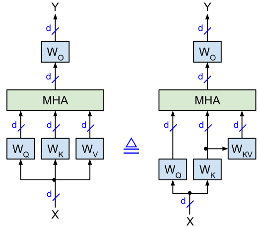
Figure 1: Mathematically identical implementations of multi-headed self-attention with square weight matrices $\in\mathbb{R}^{d\times d}$. Left: vanilla version. Right: proposed version where values V are computed from keys K with $W_{KV}=W_{K}^{-1}W_{V}$. The $\triangleq$ symbol denotes mathematical identity.

Slim attention is applicable to transformers that use MHA (multi-head attention [3]) instead of MQA (multi-query attention [4]) or GQA (grouped query attention [5]), which includes LLMs such as CodeLlama-7B and Aya-23-35B, SLMs such as Phi-3-mini and SmolLM2-1.7B, VLMs (vision language models) such as LLAVA, audio-language models such as Qwen2-Audio-7B, and encoder-decoder transformer models such as Whisper [6] and T5 [7]. Table 1 lists various MHA transformer models ranging from 9 million to 35 billion parameters. The last column of Table 1 specifies the KV-cache size (in number of activations) for each model to support its maximum context length, where the KV-cache size equals $2hd_{k}\cdot\text{layers}\cdot\text{context\_length}$.

Table 1: Various transformers with MHA (instead of MQA or GQA) and their maximum KV-cache sizes (in number of activations) based on their respective maximum context length. $h$ is the number of attention-heads, $d$ is the embedding dimension (aka hidden size), and $d_{k}$ is the head dimension. See appendix for more MHA models.

Year	Publisher	Model	Params	$d$	layers	$h$	$d_{k}$	context length	context memory
2024	Meta	CodeLlama-7B [8]	7B	4,096	32		128	16k	4.3B
		CodeLlama-13B [8]	13B	5,120	40				6.7B
	Google	CodeGemma-7B [9]	8.5B	3,072	28	16	256	8k	1.9B
	Cohere	Aya-23-35B [10]	35B	8,192	40	64	128		5.4B
	HuggingFace	SmolLM2-1.7B [11]	1.7B	2,048	24	32	64		0.8B
		SmolVLM [12]	2.3B					16k	1.6B
	Together AI	Evo-1-131k [13]	6.5B	4,096	32		128	128k	34.4B
	Microsoft	Phi-3-mini-128k [14]	3.8B	3,072	32		96		25.8B
		BitNet_b1_58-3B [15]	3.3B	3,200	26	32	100	2k	0.3B
	Apple	DCLM-7B [16]	6.9B	4,096	32		128		0.5B
	Ai2	OLMo-1B [17]	1.3B	2,048	16		128	4k	0.3B
		OLMo-2-1124-13B [17]	13.7B	5,120	40				1.7B
	Amazon	Chronos-Bolt-tiny [18]	9M	256	4		64	0.5k	1M
		Chronos-Bolt-base [18]	205M	768	12				9.4M
	Alibaba	Qwen2-Audio-7B [19]	8.4B	4,096	32		128	8k	2.1B
	LLaVA	LLaVA-NeXT-Video [20]	7.1B					4k	1.1B
2023		LLaVA-Vicuna-13B [21]	13.4B	5,120	40				1.7B
	LMSYS	Vicuna-7B-16k [22]	7B	4,096	32			16k	4.3B
		Vicuna-13B-16k [22]	13B	5,120	40				6.7B
2022	Google	Flan-T5-base [23]	248M	768	12		64	0.5k	9.4M
		Flan-T5-XXL [23]	11.3B	4,096	24	64			101M
	OpenAI	Whisper-tiny [6]	38M	384	4	6		enc: 1500 dec: 448	6M
		Whisper-large-v3 [6]	1.5B	1,280	32	20			160M
2019		GPT-2 XL [24]	1.6B	1,600	48	25		1k	157M

For long contexts, the KV-cache can be even larger than the parameter memory: For batch size 1 and 1 byte (FP8) per parameter and activation, the Phi-3-mini-128k model for example has a 3.8GB parameter memory and requires 25GB for its KV-cache to support a context length of 128K tokens. For a batch size of 16 for example, the KV-cache grows to 16 $\cdot$ 25GB = 400GB. Therefore, memory bandwidth and capacity become the bottleneck for supporting long context.

For a memory bound system with batch size 1, generating each token takes as long as reading all (activated) parameters and all KV-caches from memory. Therefore, slim attention can speed up the token generation by up to 2x for long contexts. For the Phi-3-min-128k model with 3.8GB parameters for example, slim attention reduces the KV-cache size from 25GB to 12.5GB, which reduces the total memory from 28.8GB to 16.3GB, and thus speeds up the token generation by up to 1.8x for batch size 1 (the maximum speedup happens for the generation of the very last token of the 128K tokens). And for batch size 16 for example, the speedup is (400+3.8) / (200+3.8) = 2x.

The vanilla transformer [3] defines the self-attention $Y$ of input $X$ as follows, where $h$ is the number of heads:

$$Q=XW_{Q}=\text{concat}\left(Q_{1},\ldots,Q_{h}\right)\qquad\quad K=XW_{K}=\text{concat}\left(K_{1},\ldots,K_{h}\right)$$ (1)

$$V=XW_{V}=\text{concat}\left(V_{1},\ldots,V_{h}\right)\qquad\quad Y=\text{concat}\left(\text{head}_{1},\ldots,\text{head}_{h}\right)W_{O}$$ (2)

$$\text{head}_{i}=\text{attention}\left(Q_{i},K_{i},V_{i}\right)=\text{softmax}\left(\frac{Q_{i}K_{i}^{\top}}{\sqrt{d_{k}}}\right)V_{i}$$ (3)

with $W_{Q}=\text{concat}(W_{Q,1},\ldots,W_{Q,h})$, $W_{K}=\text{concat}(W_{K,1},\ldots,W_{K,h})$, and $W_{V}=\text{concat}(W_{V,1},\ldots,W_{V,h})$, and without the causal mask for simplicity. The matrices $Q,K,V,W_{Q},W_{K}$, and $W_{V}$ are split into $h$ submatrices, one for each attention-head. Input $X$, output $Y$, queries $Q$, keys $K$, and values $V$ are $\in\mathbb{R}^{n\times d}$, where $n$ is the current sequence length (in tokens) and $d=d_{\text{model}}$ is the dimension of the embeddings.

For MHA, the weight matrices $W_{K}$ and $W_{V}$ are usually square matrices $\in\mathbb{R}^{d\times d}$, which allows us to calculate V from K as follows: Refactoring equation (1) as $X=KW_{K}^{-1}$ lets us reconstruct $X$ from $K$, which we can then plug into equation (2) to get

$$V=K(W_{K}^{-1}W_{V})=KW_{KV}\quad\text{and}\quad V_{i}=KW_{KV,i},\quad\text{where }W_{KV}=\text{concat}(W_{KV,1},\ldots,W_{KV,h})$$ (4)

and $W_{KV,i}$ $\in\mathbb{R}^{d\times d_{v}}$. Fig. 1 illustrates the modified attention scheme that calculates V from K according to equation (4). For inference, $W_{KV}=W_{K}^{-1}W_{V}$ can be precomputed offline and stored in the parameter file instead of $W_{V}$. This requires that $W_{K}$ is invertible (i.e. non-singular). In general, any square matrix can be inverted if its determinant is non-zero. It’s extremely unlikely that a large matrix has a determinant that is exactly 0.

Related work. Slim attention is somewhat similar to DeepSeek’s multi-head latent attention (MLA) [25]. Unlike MLA, slim attention is an exact post-training implementation of existing MHA models (including models with RoPE).

1 K-cache is all you need

Inference consists of the following two phases, which are illustrated in Fig. 2 for the vanilla MHA with KV-cache, where $p$ is the number of input-tokens and $n$ is the total number of current tokens including input-tokens and generated tokens, so $n=p+1,\ldots,n_{max}$ and $n_{max}$ is the context window length:

• During the prompt-phase (aka prefill phase), all $p$ input-tokens are batched up and processed in parallel. In this phase, the K and V projections are stored in the KV-cache.

• During the generate-phase (aka decoding phase), each output-token is generated sequentially (aka autoregressively). For each iteration of the generate-phase, only one new K-vector and one new V-vector are calculated and stored in the KV-cache, while all the previously stored KV-vectors are read from the cache.

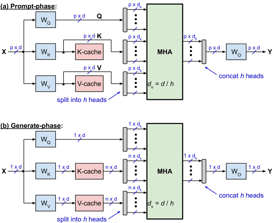
Figure 2: Standard MHA with KV-cache during (a) prompt-phase and (b) generate-phase.

Fig. 3 illustrates slim attention, which only has a K-cache because V is now calculated from K. Plugging equation (4) into (3) yields

$$\text{head}_{i}=\text{softmax}\left(\frac{Q_{i}K_{i}^{\top}}{\sqrt{d_{k}}}\right)KW_{KV,i}=\underbrace{\text{softmax}\left(\frac{Q_{i}K_{i}^{\top}}{\sqrt{d_{k}}}\right)\left[KW_{KV,i}\right]}_{\text{Option 1}}=\underbrace{\left[\text{softmax}\left(\frac{Q_{i}K_{i}^{\top}}{\sqrt{d_{k}}}\right)K\right]W_{KV,i}}_{\text{Option 2}}$$ (5)

Equation (5) can be computed in two different ways:

• Option 1 (unoptimized): Compute $V_{i}=KW_{KV,i}$ first, and then multiply it with $\text{softmax}(\cdot)$. This option is used by Fig. 3(a) and 3(b). Complexity: multiplying $K$ $\in\mathbb{R}^{n\times d}$ with $W_{KV,i}$ $\in\mathbb{R}^{d\times d_{k}}$ takes $2ndd_{k}$ OPs, and multiplying $\text{softmax}(\cdot)$ $\in\mathbb{R}^{1\times n}$ with the $n\times d_{k}$ result takes $2nd_{k}$ OPs.

• Option 2 (optimized): First multiply $\text{softmax}(\cdot)$ with $K$, and then multiply the result by $W_{KV,i}$. This option is illustrated in Fig. 3(c). During the generate-phase, this option has lower compute complexity than option 1: multiplying $\text{softmax}(\cdot)$ with $K$ takes $2nd$ OPs, and multiplying the result with $W_{KV,i}$ takes $2dd_{k}$ OPs.

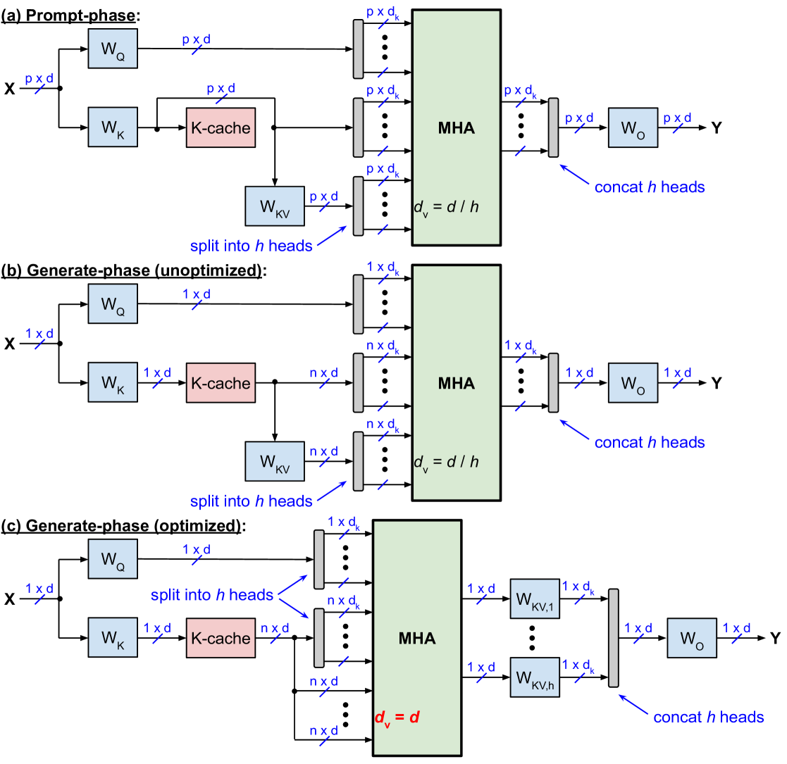
Figure 3: Slim attention without V-cache during (a) prompt-phase; (b) unoptimized and (c) optimized generate-phase.

Option 2 above uses the same associativity trick as MLA, see appendix C of [25]. During the prompt-phase, Fig. 3(a) has the same computational complexity as the vanilla scheme shown in Fig. 2(a). However, during the generate-phase, the proposed scheme has a slightly higher complexity than the vanilla scheme.

Table 2 specifies the complexity per token per layer during the generate-phase for batch size 1. The columns labeled “OPs”, “reads”, and “intensity” specify the computational complexity (as number of OPs), the number of memory reads, and the arithmetic intensity, resp. We define the arithmetic intensity here as number of OPs per each activation or parameter read from memory. Specifically, the projection complexity includes calculating $XW_{Q}$, $XW_{K}$, $XW_{V}$, and multiplying with weight matrices $W_{O}$ and $W_{KV}$. And the memory reads for projections include reading all four weight matrices; while the memory reads of the MHA include reading the K-cache (and the V-cache for the vanilla implementation). See appendix for more details on MHA complexity.

Table 2: Complexity per token per layer during the generate-phase for batch size 1

	Projection complexity			MHA complexity
	OPs	reads	intensity	OPs	reads	intensity
Vanilla, see Fig. 2(b)	$8d^{2}$	$4d^{2}$	2	$4nd$	$2nd$	2
Unoptimized, Fig. 3(b)	$(2n+6)d^{2}$	$4d^{2}$	$(n+3)/2$	$4nd$	$nd$	4
Optimized, Fig. 3(c)	$8d^{2}$	$4d^{2}$	2	$2nd(h+1)$	$nd$	$2h+2$

Note that for batch-size $B$, the arithmetic intensity of the vanilla transformer during the generate-phase is $2B$ for the FFNs and the attention-projections, but only 2 for the remaining attention operations (softmax arguments and weighted sum of V) because each of the $B$ tokens has its own KV-cache.

Table 3 shows the arithmetic intensity (now defined as OPs per memory byte) of various SoCs, TPUs, and GPUs, which vary from 93 to 583. A system is memory bound (i.e. limited by memory bandwidth) if the arithmetic intensity of the executed program is below the chip’s arithmetic intensity. Here, the maximum arithmetic intensity of slim attention is $2h+2$, see Table 2, where $h$ is the number of attention-heads, which ranges between 16 and 64 for the models listed in Table 1. So the peak arithmetic intensity (up to 130 for $h=64$) is usually less than the system’s intensity (except for Apple’s M4 Max), which means that the system is still memory bound during the token generation phase. Therefore, slim attention speeds up the processing by up to 2x as it reduces the context memory reads by half. Furthermore, slim attention enables processing all heads in parallel as a single matrix-matrix multiplication instead of multiple vector-matrix multiplications, which is usually more efficient and faster on many machines. And slim attention is also compatible with Flash Attention [26], which performs softmax and value accumulation in parallel.

Table 3: TOPS, memory bandwidth, and arithmetic intensity of popular chips

Chip	TOPS (int8)	Theoretical memory bandwidth (GB/s)	Arithmetic intensity (OPs per byte)
Rockchip RK3588	6	19	316
Apple A18 [27]	35	60	583
Apple M4 Max [27]	38	410	93
Google TPU v4 [28]	275	1,200	229
Google TPU v5p [28]	918	2,765	332
NVIDIA H200 [29]	1,980	4,800	413
NVIDIA B200 [29]	4,500	8,000	563

2 Taking advantage of softmax sparsities

In this section we describe how we can take advantage of softmax sparsities (i.e. sparsities in the attention scores) to reduce the computational complexity of the attention blocks. In some applications, many attention scores are 0 or close to zero. For those attention scores (i.e. attention scores smaller than a threshold), we can simply skip the corresponding V-vector, i.e. we don’t have to add those skipped vectors to the weighted sum of V-vectors. This reduces the complexity of calculating the weighted sum of V-vectors. For example, for a sparsity factor $S=0.8$ (i.e. 80% of scores are 0), the complexity is reduced by factor $\frac{1}{1-S}=5$.

By the way, taking advantage of softmax sparsities is also possible for systems with KV-cache where V is not computed from K. In this case, skipping V-vectors with zero scores means that we don’t have to read those V-vectors from the KV-cache, which speeds up the autoregressive generate-phase for memory bound systems. However, this will never speed it up more than slim attention’s removal of the entire V-cache. Furthermore, for MQA and GQA, each V-vector is shared among multiple (e.g. 4 or more) queries so we can only skip reading a V-vector from memory if all 4 (or more) attention scores are zero for this shared V-vector, which reduces the savings significantly. For example, if the V-vectors are shared among 4 queries and the attention scores have sparsity $S=0.8$, then the probability of all four queries being 0 is only $S^{4}=0.41$, so we can only skip 41% of the V-vectors.

3 Support for RoPE

Many transformers nowadays use RoPE (rotary positional embedding) [30], which applies positional encoding to the Q and K projections, but not the V projections. In general, RoPE can be applied to the K projections either before storing them in K-cache or after reading them from K-cache. The former is preferred because of lower computational complexity during the generate-phase (so that each K-vector is RoPE’d only once instead of multiple times). However, if the RoPE’d keys are stored in K-cache, then we first need to un-RoPE them before we can compute V from K. The following details two options to support RoPE.

Option 1 is for the case where we don’t take advantage of softmax sparsities. In this case, we apply RoPE to the K-vectors after reading them from K-cache during the generate-phase. That way we can use the raw K-vectors for computing V from K.

Option 2 is for the case where we take advantage of softmax sparsities as detailed in the previous section. In this case, RoPE is applied to the K-vectors before writing them into the K-cache. And when they are read from K-cache during the generate-phase, then we have to revert (or undo) the RoPE-encoding before we can use the K-vectors to compute the V-vectors (i.e. multiplying the K-vectors with the attention scores). However, we only need to do this for a portion of the K-vectors, depending on the sparsity factor $S$. For example, for $S=0.8$, we only need to revert the RoPE-encoding for 20% of the K-vectors. The RoPE encoding can be reverted (aka RoPE-decoding) by simply performing a rotation in the opposite direction by the same amount as shown below for the 2D case.

RoPE encoding:

$$y_{1} =x_{1}\cos{m\theta}+x_{2}\sin{m\theta}$$

$$y_{2} =-x_{1}\sin{m\theta}+x_{2}\cos{m\theta}$$

RoPE decoding:

$$x_{1} =y_{1}\cos{m\theta}-y_{2}\sin{m\theta}$$

$$x_{2} =y_{1}\sin{m\theta}+y_{2}\cos{m\theta}$$

Note that the RoPE decoding uses the same trigonometric coefficients (such as $\cos{m\theta}$) as the RoPE encoding. Therefore, we only need one look-up table that can be used for both RoPE encoding and decoding.

4 Support for bias

Since PaLM’s removal of bias terms from all its projection layers [31], most transformer models nowadays do the same. However, some models are still using biases today (especially older models that are still relevant today such as Whisper). In this section, we briefly discuss how projection layers with bias can be supported. We show how the biases of two of the four attention projection layers can be eliminated in a mathematically equivalent way.

Bias removal for V projections: This bias can be combined with the bias of the output projection layer as follows. Recall that all value vectors $v_{i}$ plus their constant bias $b$ are multiplied by the attention scores $s_{i}$ (i.e. the softmax outputs) and summed up, such as

$$\sum_{i=1}^{n}s_{i}(v_{i}+b)=\sum_{i=1}^{n}s_{i}v_{i}+\sum_{i=1}^{n}s_{i}b=\sum_{i=1}^{n}s_{i}v_{i}+b$$

The last equal sign holds because the sum over all attention-scores $s_{i}$ is always 1 as per softmax definition (because the softmax generates a probability distribution that always adds up to 1). We can now merge the bias $b$ with bias $c$ of the preceding output projection layer (O) as follows: $y=(x+b)W_{O}+c=xW_{O}+(bW_{O}+c)=xW_{O}+c^{\ast}$, with the new bias $c^{\ast}=bW_{O}+c$. This new bias-vector $c^{\ast}$ can be computed offline, before inference time. Or simply remove the V-bias already during training.

Bias removal for K projections: The bias of the K projection cancels out due to the constant invariance of the softmax function. For example, say we have 2-dimensional heads, then the dot-product $p$ between query-vector $q=(q_{1}+b_{1},q_{2}+b_{2})$ with bias $b$ and key-vector $k=(k_{1}+c_{1},k_{2}+c_{2})$ with bias $c$ is as follows:

$$p =(q_{1}+b_{1})(k_{1}+c_{1})+(q_{2}+b_{2})(k_{2}+c_{2})=[q_{1}k_{1}+q_{2}k_{2}]+[q_{1}c_{1}+q_{2}c_{2}]+[b_{1}k_{1}+b_{2}k_{2}]+[b_{1}c_{1}+b_{2}c_{2}]$$

$$=q_{1}k_{1}+q_{2}k_{2}+f(q)+b_{1}k_{1}+b_{2}k_{2}+\text{constant},$$

where $f(q)=q_{1}c_{1}+q_{2}c_{2}$ is a function of the query-vector only; and “constant” is a constant that only depends on the two biases $b$ and $c$. Now recall that the softmax function doesn’t change if a constant is added to all its arguments. Because all arguments of the attention softmax use the same single query-vector $q$, $f(q)$ is the same for all arguments and is therefore constant and can be removed from all softmax arguments. As a result, we can remove the entire bias-vector $c$ from the keys. But we still need the bias-vector $b$ for the queries. However, this assumes that there is no RoPE applied between the projections and the dot-product calculation, which is fortunately the case for Whisper for example.

5 Support for non-square weight matrices

Some transformers with MHA use non-square weight matrices for their K and V projections. Specifically, these models do not satisfy $d=d_{k}h$. The table below shows three such models where $e=d_{k}h>d$. Let’s also define the aspect ratio $r$ as $r=e/d$. For example, Google’s T5-11B model has a large aspect ratio of $r=16$.

Model	$d$	$d_{k}$	$h$	$e=d_{k}h$	aspect ratio $r=e/d$
CodeGemma-7B	3,072	256	16	4,096	1.3
T5-3B	1,024	128	32	4,096	4
T5-11B	1,024	128	128	16,384	16

There are two options to reduce the KV-cache by 2x or more, which are compared in the table below and summarized as follows:

• Option 1: Because the K weight matrix is non-square, inverting this matrix is not straight forward. And the resulting matrix $W_{KV}$ $\in\mathbb{R}^{e\times e}$, which has $r$-times more parameters than $W_{V}$ $\in\mathbb{R}^{d\times e}$.

• Option 2: Instead of storing V in cache and then calculating V from K, we can store the smaller $d$-element vectors X before the projection and then on-the-fly calculate both projections (V and K) from X. The cache is now $r$-times smaller than option 1, and $2r$ times smaller than the baseline, for example 32 times smaller for the T5-11B model. However, this comes at a slightly higher computational cost.

	Baseline	Option 1	Option 2
Cache reduction factor	1	2	$2r$
Size of $W_{V}$ or $W_{KV}$	$de$	$e^{2}$ ($r$-times larger)	$de$
Computational complexity	baseline	higher	even higher
Support for RoPE?	Yes	Yes	No

Option 1: The standard matrix inverse is defined only for square matrices, and the inversion functions in NumPy and SciPy are limited to such matrices. We want to compute the inverse of $W_{K}$ $\in\mathbb{R}^{d\times e}$ with $e>d$ such that $W_{K}W_{K}^{-1}=I$, where $I$ is the identity matrix and $W_{K}^{-1}$ is the so-called right inverse of $W_{K}$. We compute $W_{K}^{-1}$ by using a trick that inverts the term $W_{K}W_{K}^{\top}$ instead of $W_{K}$ as follows:

$$I=W_{K}\underbrace{W_{K}^{\top}(W_{K}W_{K}^{\top})^{-1}}_{W_{K}^{-1}}$$

In the equation above, everything on the right side of $W_{K}$ has to be the inverse of $W_{K}$, thus $W_{K}^{-1}=W_{K}^{\top}(W_{K}W_{K}^{\top})^{-1}$. We can now use the matrix inversion function of NumPy to compute the inverse of the term $W_{K}W_{K}^{\top}$, which is a square $d\times d$ matrix. Now we can calculate $W_{KV}=W_{K}^{-1}W_{V}$. However, storing $W_{KV}$ instead of the original $W_{V}$ takes $r$ times more space in memory, which is an issue for large aspect-ratios $r$.

Option 2 caches the X-matrix instead of KV or just K, where the X-matrix contains the input activations of the attention layer (before the projections). Recomputing all K-vectors from X by multiplying X with weight matrix $W_{K}$ would require $2nde$ operations and would be very expensive. A lower complexity option is illustrated in Fig. 4, which is similar to the trick illustrated in Fig. 3(c).

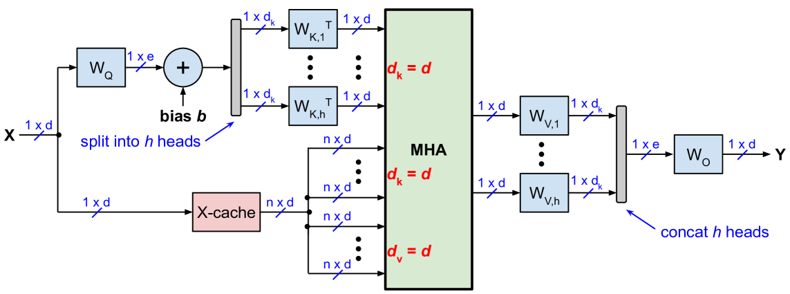
Figure 4: Slim attention with X-cache (instead of KV or V-cache) for the generate-phase of transformers with non-square weight matrices with $e>d$.

Recall that for the $i$-th head ($i=1,\ldots,h$), the softmax argument (without the scaling factor $1/\sqrt{d_{k}}$) is $A_{i}=Q_{i}K_{i}^{\top}$, where $Q_{i}=XW_{Q,i}$ and $K_{i}=XW_{K,i}$. For the generate-phase, there is only one input-vector $x_{n}$ for the query, but there are $n$ input-vectors $X$ for the key and value projections. We can take advantage of this and modify $A$ as follows (which uses the trick $(BC)^{\top}=C^{\top}B^{\top}$ for transposing the product of arbitrary matrices $B$ and $C$):

$$A_{i}=Q_{i}K_{i}^{\top}=x_{n}W_{Q,i}(XW_{K,i})^{\top}=(x_{n}W_{Q,i}W_{K,i}^{\top})X^{\top}$$

For each iteration of the generate-phase, we now have to calculate the term $x_{n}W_{Q,i}W_{K,i}^{\top}$ only once for each attention-head, which is independent of the sequence length. Calculating this term involves multiplying the $d$-dimensional vector $x_{n}$ with matrices $W_{Q,i}$ $\in\mathbb{R}^{d\times d_{k}}$ and $W_{K,i}^{\top}$ $\in\mathbb{R}^{d_{k}\times d}$, which requires $2de$ multiplications for the $h$ heads, so $4de$ operations in total (where we count a multiply-add operation as 2 operations).

This scheme also works for projection layers with biases (as used by the Whisper models for example). Recall from the previous section that we can eliminate the biases from the key and value projections, but not from the query projection. Adding a constant query bias-vector $b$ to the equation above is straightforward and also illustrated in Fig. 4:

$$A_{i}=Q_{i}K_{i}^{\top}=(x_{n}W_{Q,i}+b)(XW_{K,i})^{\top}=((x_{n}W_{Q,i}+b)W_{K,i}^{\top})X^{\top}$$

However, this scheme doesn’t work if there is a positional encoding such as RoPE located between the projection layers and the dot-product calculation. But option 2 fully supports other relative position encoding (PE) schemes such as RPE of the T5 model, Alibi, Kerple and FIRE [32] which add a variable bias to the softmax arguments (instead of modifying the queries and keys before the dot-product calculation). See for example the FIRE paper [32], which shows that FIRE and even NoPE can outperform RoPE for long context.

6 Support for encoder-decoder transformers

In general, calculating K from V is not only possible for self-attention (see Fig. 1) but also for cross-attention. In this section, we present two context memory options for encoder-decoder transformers such as Whisper (speech-to-text), language translation models such as Google’s T5, and time series forecasting models such as Amazon’s Chronos models. One option is not limited to MHA only, but is also applicable to MQA and GQA. The table below compares the options, which are summarized as follows:

• The baseline implementation uses complete KV-caches for both self-attention and cross-attention of the decoder stack, which we refer to as self KV-cache and cross KV-cache, resp.

• Option 1 is an optimized implementation where the V-caches for both self-attention and cross-attention are eliminated, which reduces the total cache size by 2x.

• Option 2 eliminates the entire cross KV-cache and also eliminates the V-cache of the self-attention.

The baseline implementation consists of the following three phases:

• During the prompt-phase, only the encoder is active. All $p$ input-tokens are batched up and processed in parallel. This phase is identical to the prompt-phase of a decoder-only transformer albeit without a causal mask (and is also identical to the entire inference of an encoder-only transformer such as BERT).

• During the cross-phase, we take the output of the encoder (which is a $p\times d$ matrix) and precompute the KV projections for the decoder’s cross-attention and store them in cross context memory (aka cross KV-cache).

• The generate-phase is similar to the generate-phase of a decoder-only transformer with the following difference: There is a cross-attention block for each layer, which reads keys and values from the cross KV-cache. In addition, the self-attention blocks have their own self KV-cache (which is not the same as the cross KV-cache).

	Baseline	Option 1	Option 2
Self KV-cache size	100%	50%	50%
Cross KV-cache size	100%	50%	0
Need to read cross-$W_{K}$ and $W_{V}$ during the generate-phase?	No	$W_{KV}$ only	$W_{K}$ and $W_{V}$
Support for RoPE?	Yes	Yes	No
Complexity of cross-phase	full	half	0

Option 1 calculates V from K for both self-attention and cross-attention of the decoder stack (note that the encoder stack doesn’t have a KV-cache because it is not autoregressive). This requires reading the cross-$W_{KV}$ parameters from memory during the generate-phase. So if the $W_{KV}$ matrices are larger than the cross V-cache, then calculating V from K for the cross-attention doesn’t make sense for batch size 1 (but for larger batch sizes). For the Whisper models for example, the cross V-cache is always larger than the $W_{KV}$ matrices, because the number of encoder-tokens $p$ is always 1500. And for batch sizes $B$ larger than 1, the reading of the cross-$W_{KV}$ parameters can be amortized among the $B$ inferences.

Option 2 efficiently recomputes the cross KV-projections from the encoder output instead of storing them in the cross KV-cache as follows:

• At the end of the prompt-phase, the encoder output is a $p\times d$ matrix, which is then used by all layers of the decoder stack. We call this matrix $E$ $\in\mathbb{R}^{p\times d}$ the encoder-cache (or E-cache) and we assume that it resides in on-chip SRAM (such as L2 or L3 cache) at the end of the prompt-phase, because it’s usually very small (less than 1 million values for Whisper tiny and base for example).

• Recomputing all K-vectors could be done by multiplying $E$ $\in\mathbb{R}^{p\times d}$ with weight matrix $W_{K}$ $\in\mathbb{R}^{d\times d}$, which requires $2pd^{2}$ operations and would be very expensive. A lower complexity option is illustrated in Fig. 5, which is similar to Fig. 4. The main difference is that all cross-attention layers share the same E-cache. And on many machines, this E-cache might fit into on-chip SRAM so that it doesn’t need to be re-read for each layer during the generate-phase.

• As with Fig. 4 in the previous section, Fig. 5 doesn’t support RoPE, but other (and potentially better) relative PE schemes such as RPE, FIRE, and NoPE.

• This scheme doesn’t calculate V from K and therefore is not limited to MHA only or to projection matrices that can be inverted.

• Similar to option 1 (and unlike the baseline), the cross-$W_{V}$ and $W_{K}$ parameters need to be read from memory for each generated token during the generate-phase. Therefore for batch size 1, this scheme only makes sense if the KV-cache is larger than the number of cross-$W_{V}$ and $W_{K}$ parameters, which is the case for all Whispers models (because they use $p=1500$ input-tokens, and $d$ of the largest Whisper model is smaller than 1500). And for batch sizes larger than 1, this option usually makes sense because the parameter reads are amortized among all the inferences of the batch.

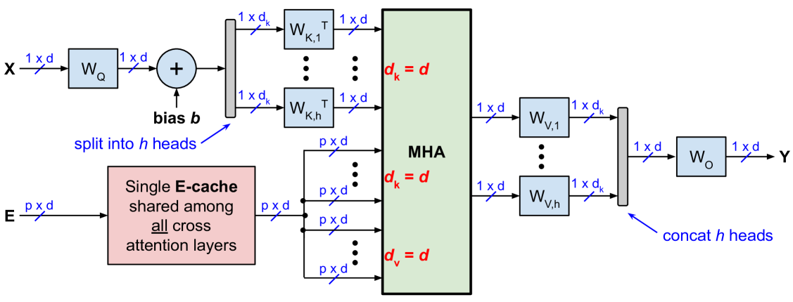
Figure 5: Slim attention with a single X-cache that is shared among all cross-attention layers for the generate-phase of encoder-decoder transformers.

Time-to-first-token (TTFT): Options 1 and 2 speed up or eliminate the cross-phase. Specifically, option 1 speeds up the cross-phase by 2x. And option 2 completely eliminates the cross-phase. This speeds up the time-to-first-token latency (TTFT). And in certain cases, the overall compute complexity can be reduced compared to the baseline. For cases where the number of encoder-tokens is larger than the decoder-tokens (such as for Whisper or for text summarization) and for large $d$ dimensions, these options can reduce the overall complexity.

The table below lists the cache size savings and speedups during the generate-phase for all 5 Whisper models, assuming a fixed encoder context length of $p=1500$, a decoder output context length of 448, and a vocab_size of 51,865. Option 2 reduces the cache sizes by 8.7x, assuming that the entire encoder output (matrix E) is kept in on-chip SRAM (the E-cache), which speeds up the generate-phase by over 5x for a memory bound system with batch size 64. Note that the speedups listed in the table are in addition to speeding up the cross-phase (i.e. 2x cross-phase speedup for option 1, and entire elimination of the cross-phase for option 2).

	Whisper models
	tiny	base	small	medium	large	Notes
Params	38M	73M	242M	764M	1.5B	number of parameters
Layers	4	6	12	24	32	number of layers
$d$	384	512	768	1,024	1,280	embedding dimension
$d_{\text{ffn}}$	1,536	2,048	3,072	4,096	5,120	hidden dimension of FFN
Cache sizes (in M):
Encoder E-cache	0.6	0.8	1.2	1.5	1.9	$1500\cdot d$
Cross KV-cache	4.6	9.2	27.6	73.7	122.9	$2\cdot 1500\cdot d\cdot\text{layers}$
Self KV-cache	1.4	2.8	8.3	22.0	36.7	$2\cdot 448\cdot d\cdot\text{layers}$
Baseline cache	6.0	12.0	35.9	95.7	159.6	cross KV + self KV
Option 1 cache	3.0	6.0	18.0	47.9	79.8	half of baseline
Option 2 cache	0.7	1.4	4.1	11.0	18.4	no cross KV + half of self KV-cache
Option 2 savings	8.7x	8.7x	8.7x	8.7x	8.7x	cache savings vs. baseline
Number of parameters (in M) for generate-phase:
Baseline params	28.2	48.6	138.9	405.4	800.4	$d\cdot\text{vocab}+\text{layers}\cdot(6d^{2}+2d\cdot d_{\text{ffn}})$
Option 1 params	28.8	50.1	146.0	430.6	852.8	baseline + cross K ($d^{2}\cdot\text{layers}$)
Option 2 params	29.4	51.7	153.1	455.8	905.2	baseline + cross KV ($2d^{2}\cdot\text{layers}$)
Memory reads (in M) per token for batch size 1:
Baseline	34.2	60.5	174.8	501.2	960.0	baseline cache + baseline params
Option 1	31.8	56.1	164.0	478.5	932.6	option 1 cache + option 1 params
Option 2	30.0	53.1	157.2	466.8	923.6	option 2 cache + option 2 params
Option 1 speedup	1.08x	1.08x	1.07x	1.05x	1.03x	speedup vs. baseline
Option 2 speedup	1.14x	1.14x	1.11x	1.07x	1.04x	speedup vs. baseline
Memory reads (in M) per token for batch size 64:
Baseline	6.4	12.7	38.1	102.1	172.1	baseline cache + $1/64\cdot$ params
Option 1	3.4	6.8	20.2	54.6	93.1	option 1 cache + $1/64\cdot$ params
Option 2	1.1	2.2	6.5	18.1	32.5	option 2 cache + $1/64\cdot$ params
Option 1 speedup	1.9x	1.9x	1.9x	1.9x	1.8x	speedup vs. baseline
Option 2 speedup	5.6x	5.8x	5.8x	5.6x	5.3x	speedup vs. baseline

There is a further optimization, which is a hybrid of options 1 and 2, where one layer of the decoder stack uses option 1 and the other layers use a modified version of option 2 as follows: Say the first layer implements option 1, which entails calculating and storing the cross K-cache for the first layer, i.e. $K=EW_{K}$. The trick is now to use this K-cache instead of the E-cache for all the other layers and then we can calculate E from K as $E=KW_{K\_layer1}^{-1}$. So the other layers will now use K instead of E, which means that they need to use modified versions of their $W_{K}$ and $W_{V}$ weight matrices, which are offline computed as $W_{V\_new}=W_{K\_layer1}^{-1}W_{V\_old}$ and $W_{K\_new}=W_{K\_layer1}^{-1}W_{K\_old}$. The savings of this hybrid versus option 2 are not huge: It only speeds up the first layer because we only need to read one of the two cross weight matrices for the first layer for each generated token (i.e. we only need to read $W_{KV\_layer1}$ instead of reading both $W_{K\_layer1}$ and $W_{V\_layer1}$). So this hybrid makes only sense for shallow models, e.g. Whisper tiny which only has 4 layers.

7 Conclusion

Slim attention offers a simple trick for halving the context memory of existing MHA transformer models without sacrificing accuracy. Slim attention is a post-training, exact implementation of existing models, so it doesn’t require any fine-tuning or training from scratch. Future work includes integrating slim attention into popular frameworks such as HuggingFace Transformers [33], llama.cpp [34], vLLM [35], llamafile [36], LM Studio [37], Ollama [38], SGLang [39], and combining it with existing context memory management schemes such as PagedAttention [40] and other compression schemes such as Dynamic Memory Compression DMC [41] and VL-cache [42]. Please also see our forthcoming paper about matrix-shrink [43], which reduces the sizes of attention matrices and proposes a simplification of DeepSeek’s MLA scheme.

Appendix

MHA complexity

This section derives the number of OPs (two-operand operations) for the column labeled “MHA complexity” of Table 2, which is the MHA-complexity per token during the generate-phase. Recall that multiplying two matrices (MatMul) with dimensions $m\times n$ and $n\times p$ entails computing $mp$ dot-products of length $n$, where each dot-product takes $n$ MULs (two-operand multiply operations) and $n-1$ ADDs (two-operand add operations). In total, the entire MatMul requires $mnp$ MULs and $mp(n-1)$ ADDs, so $mp(2n-1)$ OPs, which is approximately $2mnp$ OPs.

	Term	Dimensions of MatMul	OPs per attention-head
Softmax argument	$Q_{i}K_{i}^{\top}$	$(1\times d_{k})(d_{k}\times n)$	$2nd_{k}$
Weighted sum of $V_{i}$	$\text{softmax}()\cdot V_{i}$	$(1\times n)(n\times d_{k})$	$2nd_{k}$
Weighted sum of $K$	$\text{softmax}()\cdot K$	$(1\times n)(n\times d)$	$2nd$

The table above specifies the number of OPs per attention-head for computing the softmax arguments and the weighted sums. This is for the generate-phase where all MatMuls are actually vector-matrix products.

The table below shows the total number of MHA OPs across all attention-heads for the three cases of Table 2 (i.e. for Vanilla, unoptimized Fig. 3(b), and optimized Fig. 3(c)). Note that $d_{k}=d/h$.

	OPs per attention-head
	softmax argument	weighted sum	Total OPs
Vanilla, see Fig. 2(b)	$2nd_{k}$	$2nd_{k}$	$h(2nd_{k}+2nd_{k})=4nd$
Unoptimized, Fig. 3(b)	$2nd_{k}$	$2nd_{k}$	$4nd$
Optimized, Fig. 3(c)	$2nd_{k}$	$2nd$	$h(2nd_{k}+2nd)=2nd(h+1)$

Alternative scheme: all you need is V-cache

Instead of calculating V from K, it’s also possible to calculate K from V and thereby eliminate the K-cache (instead of the V-cache). This alternative scheme is illustrated in Fig. 6, where $W_{VK}=W_{V}^{-1}W_{K}$. However, this scheme does not support RoPE.

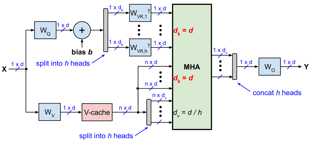
Figure 6: Alternative scheme during generate-phase

Slim Attention for GQA (such as Gemma2-9B)

Slim attention is not limited to MHA only. In general, slim attention reduces the KV-cache size whenever the width of the KV-cache ($d_{\text{cache}}$) is larger than $d_{\text{model}}$, where $d_{\text{cache}}=h_{KV}(d_{K}+d_{V})$, where $h_{KV}$ is the number of KV-heads. In this case, slim attention can compress the KV-cache size by the compression factor $c=d_{\text{cache}}/d_{\text{model}}$. Usually, this compression factor $c$ is 2. In some cases, $c$ is larger than 2, for example CodeGemma-7B has $c=2*4096/3072=2.67$.

For Gemma2-9B and PaliGemma2-10B, which utilize GQA instead of MHA, $c=2*2048/3584=1.14$. In this case where the compression factor $c$ is smaller than 2 and larger than 1, the application of slim attention is not straight forward. The figure below shows how we can implement slim attention for this case, where $e=h_{KV}d_{K}$ is the projection dimension of the $d\times e$ weight matrices and $d/2<e<d$. For Gemma2-9B, $e=2048$ and $d=3584$. Note that $W_{K}^{\ast}$ has $d^{2}$ parameters, while the original $W_{K}$ has only $de$ parameters, which is a disadvantage.

More MHA models

The table below lists additional transformer models with MHA, similar to Table 1. See HuggingFace for more details on these models.

Year	Publisher	Model	Params	$d$	layers	$h$	$d_{k}$
2025	Metagene	METAGENE-1 [44]	6.5B	4096	32	32	128
2025	Ai2	OLMoE-1B-7B-0125 [45]	6.9B	2048	16	16	128
2025	Meta	DRAMA-base [46]	212M	768	12	12	64
2024	Meta	Chameleon-7B [47]	7B	4096	32	32	128
2024	Meta	llm-compiler-13B [48]	13B	5120	40	40	128
2024	DeepSeek	DeepSeek-vl2-tiny	3.4B	1280	12	10	128
2024	nyra health	CrisperWhisper [49]	1.6B	1280	32	20	64
2024	Useful Sensors	Moonshine-base [50]	61M	416	8	8	52
2024	Moondream	Moondream-2	1.9B	2048	24	32	64
2024	Stability AI	Stable-Code-3B [51]	2.8B	2560	32	32	80
2024	Stability AI	Stable-LM2-1.6B [52]	1.6B	2048	24	32	64
2024	NVIDIA	OpenMath-CodeLlama-13B [53]	13B	5120	40	40	128
2024	Microsoft	MAIRA-2 [54]	6.9B	4096	32	32	128
2024	Pansophic	Rocket-3B	2.8B	2560	32	32	80
2024	OpenLM Research	OpenLLaMA-13B	13B	5120	40	40	128
2024	Google	TimesFM-1.0-200M [55]	200M	1280	20	16	80
2024	Google	MetricX-24-hybrid-XXL [56]	13B	4096	24	64	64
2024	Stanford	BioMedLM [57]	2.7B	2560	32	20	128
2024	OpenBMB	MiniCPM-V2 [58]	3.4B	2304	40	36	64
2023	OpenBMB	UltraLM-65B	65B	8192	80	64	128
2023	Together AI	LLaMA-2-7B-32K	7B	4096	32	32	128
2023	Databricks	Dolly-v2-12B	12B	5120	36	40	128
2023	Mosaic ML	MPT-7B-8K	7B	4096	32	32	128
2023	Mosaic ML	MPT-30B	30B	7168	48	64	112
2022	BigScience	BLOOM [59]	176B	14,336	70	112	128

References

- OpenMachine [2024] OpenMachine. Transformer tricks. 2024. URL https://github.com/OpenMachine-ai/transformer-tricks.
- Andrew Wasielewski with audio generated by Notebook LM [2025] Andrew Wasielewski with audio generated by Notebook LM. Podcast-video about Slim Attention. Jan 2025.
- Vaswani et al. [2017] Ashish Vaswani, Noam Shazeer, Niki Parmar, Jakob Uszkoreit, Llion Jones, Aidan N Gomez, Lukasz Kaiser, and Illia Polosukhin. Attention is all you need. June 2017. arXiv:1706.03762.
- Shazeer [2019] Noam Shazeer. Fast Transformer Decoding: One Write-Head is All You Need. November 2019. arXiv:1911.02150.
- Ainslie et al. [2023] Joshua Ainslie, James Lee-Thorp, Michiel de Jong, Yury Zemlyanskiy, Federico Lebrón, and Sumit Sanghai. GQA: Training generalized multi-query transformer models from multi-head checkpoints. May 2023. arXiv:2305.13245.
- Radford et al. [2022] Alec Radford, Jong Wook Kim, Tao Xu, Greg Brockman, Christine McLeavey, and Ilya Sutskever. Robust speech recognition via large-scale weak supervision. December 2022. arXiv:2212.04356.
- Raffel et al. [2019] Colin Raffel, Noam Shazeer, Adam Roberts, Katherine Lee, Sharan Narang, Michael Matena, Yanqi Zhou, Wei Li, and Peter J Liu. Exploring the limits of transfer learning with a unified text-to-text transformer. October 2019. arXiv:1910.10683.
- Rozière et al. [2023] Baptiste Rozière, Jonas Gehring, Fabian Gloeckle, Sten Sootla, Itai Gat, Xiaoqing Ellen Tan, Yossi Adi, Jingyu Liu, Romain Sauvestre, Tal Remez, Jérémy Rapin, Artyom Kozhevnikov, Ivan Evtimov, Joanna Bitton, Manish Bhatt, Cristian Canton Ferrer, Aaron Grattafiori, Wenhan Xiong, Alexandre Défossez, Jade Copet, Faisal Azhar, Hugo Touvron, Louis Martin, Nicolas Usunier, Thomas Scialom, and Gabriel Synnaeve. Code Llama: Open foundation models for code. August 2023. arXiv:2308.12950.
- CodeGemma Team et al. [2024] CodeGemma Team, Heri Zhao, Jeffrey Hui, Joshua Howland, Nam Nguyen, Siqi Zuo, Andrea Hu, Christopher A Choquette-Choo, Jingyue Shen, Joe Kelley, Kshitij Bansal, Luke Vilnis, Mateo Wirth, Paul Michel, Peter Choy, Pratik Joshi, Ravin Kumar, Sarmad Hashmi, Shubham Agrawal, Zhitao Gong, Jane Fine, Tris Warkentin, Ale Jakse Hartman, Bin Ni, Kathy Korevec, Kelly Schaefer, and Scott Huffman. CodeGemma: Open Code Models Based on Gemma. June 2024. arXiv:2406.11409.
- Aryabumi et al. [2024] Viraat Aryabumi, John Dang, Dwarak Talupuru, Saurabh Dash, David Cairuz, Hangyu Lin, Bharat Venkitesh, Madeline Smith, Jon Ander Campos, Yi Chern Tan, Kelly Marchisio, Max Bartolo, Sebastian Ruder, Acyr Locatelli, Julia Kreutzer, Nick Frosst, Aidan Gomez, Phil Blunsom, Marzieh Fadaee, Ahmet Üstün, and Sara Hooker. Aya 23: Open weight releases to further multilingual progress, May 2024. arXiv:2405.15032.
- Allal et al. [2024] Loubna Ben Allal, Anton Lozhkov, Elie Bakouch, Gabriel Martín Blázquez, Lewis Tunstall, Agustín Piqueres, Andres Marafioti, Cyril Zakka, Leandro von Werra, and Thomas Wolf. SmolLM2 - with great data, comes great performance, 2024. URL https://huggingface.co/HuggingFaceTB/SmolLM2-1.7B.
- Marafioti et al. [2024] Andres Marafioti, Merve Noyan, Miquel Farré, Elie Bakouch, and Pedro Cuenca. SmolVLM - small yet mighty Vision Language Model. November 2024. HuggingFace blog.
- Nguyen et al. [2024] Eric Nguyen, Michael Poli, Matthew G. Durrant, Brian Kang, Dhruva Katrekar, David B. Li, Liam J. Bartie, Armin W. Thomas, Samuel H. King, Garyk Brixi, Jeremy Sullivan, Madelena Y. Ng, Ashley Lewis, Aaron Lou, Stefano Ermon, Stephen A. Baccus, Tina Hernandez-Boussard, Christopher Ré, Patrick D. Hsu, and Brian L. Hie. Sequence modeling and design from molecular to genome scale with Evo. Science, 386(6723), 2024.
- Abdin et al. [2024] Marah Abdin, Jyoti Aneja, Hany Awadalla, Ahmed Awadallah, Ammar Ahmad Awan, Nguyen Bach, Amit Bahree, Arash Bakhtiari, Jianmin Bao, Harkirat Behl, Alon Benhaim, Misha Bilenko, Johan Bjorck, Sébastien Bubeck, Martin Cai, Qin Cai, Vishrav Chaudhary, Dong Chen, Dongdong Chen, Weizhu Chen, Yen-Chun Chen, Yi-Ling Chen, Hao Cheng, Parul Chopra, Xiyang Dai, Matthew Dixon, Ronen Eldan, Victor Fragoso, Jianfeng Gao, Mei Gao, Min Gao, et al. Phi-3 technical report: A highly capable language model locally on your phone. April 2024. arXiv:2404.14219.
- Ma et al. [2024] Shuming Ma, Hongyu Wang, Lingxiao Ma, Lei Wang, Wenhui Wang, Shaohan Huang, Li Dong, Ruiping Wang, Jilong Xue, and Furu Wei. The Era of 1-bit LLMs: All Large Language Models are in 1.58 Bits. February 2024. arXiv:2402.17764.
- Li et al. [2024] Jeffrey Li, Alex Fang, Georgios Smyrnis, Maor Ivgi, Matt Jordan, Samir Gadre, Hritik Bansal, Etash Guha, Sedrick Keh, Kushal Arora, Saurabh Garg, Rui Xin, Niklas Muennighoff, Reinhard Heckel, Jean Mercat, Mayee Chen, Suchin Gururangan, Mitchell Wortsman, Alon Albalak, Yonatan Bitton, Marianna Nezhurina, Amro Abbas, Cheng-Yu Hsieh, Dhruba Ghosh, Josh Gardner, Maciej Kilian, Hanlin Zhang, Rulin Shao, Sarah Pratt, Sunny Sanyal, Gabriel Ilharco, Giannis Daras, Kalyani Marathe, Aaron Gokaslan, Jieyu Zhang, Khyathi Chandu, Thao Nguyen, Igor Vasiljevic, Sham Kakade, Shuran Song, Sujay Sanghavi, Fartash Faghri, Sewoong Oh, Luke Zettlemoyer, Kyle Lo, Alaaeldin El-Nouby, Hadi Pouransari, Alexander Toshev, Stephanie Wang, Dirk Groeneveld, Luca Soldaini, Pang Wei Koh, Jenia Jitsev, Thomas Kollar, Alexandros G. Dimakis, Yair Carmon, Achal Dave, Ludwig Schmidt, and Vaishaal Shankar. DataComp-LM: In search of the next generation of training sets for language models, 2024. arXiv:2406.11794.
- Groeneveld et al. [2024] Dirk Groeneveld, Iz Beltagy, Pete Walsh, Akshita Bhagia, Rodney Kinney, Oyvind Tafjord, Ananya Harsh Jha, Hamish Ivison, Ian Magnusson, Yizhong Wang, Shane Arora, David Atkinson, Russell Authur, Khyathi Raghavi Chandu, Arman Cohan, Jennifer Dumas, Yanai Elazar, Yuling Gu, Jack Hessel, Tushar Khot, William Merrill, Jacob Morrison, Niklas Muennighoff, Aakanksha Naik, Crystal Nam, Matthew E Peters, Valentina Pyatkin, Abhilasha Ravichander, Dustin Schwenk, Saurabh Shah, Will Smith, Emma Strubell, Nishant Subramani, Mitchell Wortsman, Pradeep Dasigi, Nathan Lambert, Kyle Richardson, Luke Zettlemoyer, Jesse Dodge, Kyle Lo, Luca Soldaini, Noah A Smith, and Hannaneh Hajishirzi. OLMo: Accelerating the science of language models. February 2024. arXiv:2402.00838.
- Ansari et al. [2024] Abdul Fatir Ansari, Lorenzo Stella, Caner Turkmen, Xiyuan Zhang, Pedro Mercado, Huibin Shen, Oleksandr Shchur, Syama Sundar Rangapuram, Sebastian Pineda Arango, Shubham Kapoor, Jasper Zschiegner, Danielle C Maddix, Hao Wang, Michael W Mahoney, Kari Torkkola, Andrew Gordon Wilson, Michael Bohlke-Schneider, and Yuyang Wang. Chronos: Learning the language of time series. March 2024. arXiv:2403.07815.
- Chu et al. [2024] Yunfei Chu, Jin Xu, Qian Yang, Haojie Wei, Xipin Wei, Zhifang Guo, Yichong Leng, Yuanjun Lv, Jinzheng He, Junyang Lin, Chang Zhou, and Jingren Zhou. Qwen2-Audio Technical Report. July 2024. arXiv:2407.10759.
- Zhang et al. [2024] Yuanhan Zhang, Bo Li, haotian Liu, Yong jae Lee, Liangke Gui, Di Fu, Jiashi Feng, Ziwei Liu, and Chunyuan Li. LLaVA-NeXT: A Strong Zero-shot Video Understanding Model. April 2024.
- Liu et al. [2023] Haotian Liu, Chunyuan Li, Yuheng Li, and Yong Jae Lee. Improved baselines with visual instruction tuning. October 2023. arXiv:2310.03744.
- Chiang et al. [2023] Wei-Lin Chiang, Zhuohan Li, Zi Lin, Ying Sheng, Zhanghao Wu, Hao Zhang, Lianmin Zheng, Siyuan Zhuang, Yonghao Zhuang, Joseph E. Gonzalez, Ion Stoica, and Eric P. Xing. Vicuna: An Open-Source Chatbot Impressing GPT-4 with 90%* ChatGPT Quality. March 2023.
- Chung et al. [2022] Hyung Won Chung, Le Hou, Shayne Longpre, Barret Zoph, Yi Tay, William Fedus, Yunxuan Li, Xuezhi Wang, Mostafa Dehghani, Siddhartha Brahma, Albert Webson, Shixiang Shane Gu, Zhuyun Dai, Mirac Suzgun, Xinyun Chen, Aakanksha Chowdhery, Alex Castro-Ros, Marie Pellat, Kevin Robinson, Dasha Valter, Sharan Narang, Gaurav Mishra, Adams Yu, Vincent Zhao, Yanping Huang, Andrew Dai, Hongkun Yu, Slav Petrov, Ed H Chi, Jeff Dean, Jacob Devlin, Adam Roberts, Denny Zhou, Quoc V Le, and Jason Wei. Scaling instruction-finetuned language models. October 2022. arXiv:2210.11416.
- Radford et al. [2019] Alec Radford, Jeff Wu, Rewon Child, David Luan, Dario Amodei, and Ilya Sutskever. Language Models are Unsupervised Multitask Learners. 2019.
- [25] DeepSeek-AI, Aixin Liu, Bei Feng, Bin Wang, Bingxuan Wang, Bo Liu, Chenggang Zhao, Chengqi Dengr, Chong Ruan, Damai Dai, Daya Guo, Dejian Yang, Deli Chen, Dongjie Ji, Erhang Li, Fangyun Lin, Fuli Luo, Guangbo Hao, Guanting Chen, Guowei Li, H. Zhang, Hanwei Xu, Hao Yang, Haowei Zhang, Honghui Ding, Huajian Xin, Huazuo Gao, Hui Li, Hui Qu, J. L. Cai, Jian Liang, Jianzhong Guo, Jiaqi Ni, Jiashi Li, Jin Chen, Jingyang Yuan, Junjie Qiu, et al. DeepSeek-V2: A Strong, Economical, and Efficient Mixture-of-Experts Language Model.
- Dao et al. [2022] Tri Dao, Daniel Y Fu, Stefano Ermon, Atri Rudra, and Christopher Ré. FlashAttention: Fast and memory-efficient exact attention with IO-awareness. May 2022. arXiv:2205.14135.
- Wikipedia [2025a] Wikipedia. Apple silicon, 2025a. Accessed Jan-2025.
- Wikipedia [2025b] Wikipedia. Tensor Processing Unit, 2025b. Accessed Jan-2025.
- Wikipedia [2025c] Wikipedia. Nvidia DGX, 2025c. Accessed Jan-2025.
- Su et al. [2021] Jianlin Su, Yu Lu, Shengfeng Pan, Ahmed Murtadha, Bo Wen, and Yunfeng Liu. RoFormer: Enhanced transformer with Rotary Position Embedding. April 2021. arXiv:2104.09864.
- Chowdhery et al. [2022] Aakanksha Chowdhery, Sharan Narang, Jacob Devlin, Maarten Bosma, Gaurav Mishra, Adam Roberts, Paul Barham, Hyung Won Chung, Charles Sutton, Sebastian Gehrmann, Parker Schuh, Kensen Shi, Sasha Tsvyashchenko, Joshua Maynez, Abhishek Rao, Parker Barnes, Yi Tay, Noam Shazeer, et al. PaLM: Scaling language modeling with Pathways. April 2022. arXiv:2204.02311.
- Li et al. [2023] Shanda Li, Chong You, Guru Guruganesh, Joshua Ainslie, Santiago Ontanon, Manzil Zaheer, Sumit Sanghai, Yiming Yang, Sanjiv Kumar, and Srinadh Bhojanapalli. Functional interpolation for relative positions improves long context Transformers. October 2023. arXiv:2310.04418.
- [33] HuggingFace. Transformers. URL https://huggingface.co/docs/transformers.
- [34] Georgi Gerganov. llama.cpp. URL https://github.com/ggerganov/llama.cpp.
- [35] vLLM Project. vLLM. URL https://github.com/vllm-project/vllm.
- [36] Mozilla. llamafile. URL https://github.com/Mozilla-Ocho/llamafile.
- [37] LM Studio. LM Studio. URL https://lmstudio.ai.
- [38] Ollama. Ollama. URL https://github.com/ollama/ollama.
- [39] SGLang. SGLang. URL https://github.com/sgl-project/sglang.
- Kwon et al. [2023] Woosuk Kwon, Zhuohan Li, Siyuan Zhuang, Ying Sheng, Lianmin Zheng, Cody Hao Yu, Joseph E Gonzalez, Hao Zhang, and Ion Stoica. Efficient memory management for large language model serving with PagedAttention. September 2023. arXiv:2309.06180.
- Nawrot et al. [2024] Piotr Nawrot, Adrian Łańcucki, Marcin Chochowski, David Tarjan, and Edoardo M. Ponti. Dynamic Memory Compression: Retrofitting LLMs for Accelerated Inference. 2024. arXiv:2403.09636.
- Tu et al. [2024] Dezhan Tu, Danylo Vashchilenko, Yuzhe Lu, and Panpan Xu. VL-cache: Sparsity and modality-aware KV cache compression for vision-language model inference acceleration. October 2024. arXiv:2410.23317.
- Graef [2025] Nils Graef. Matrix-shrink for transformers without loss of accuracy. 2025. URL https://github.com/OpenMachine-ai/transformer-tricks/blob/main/doc/matShrink.pdf.
- Liu et al. [2025] Ollie Liu, Sami Jaghouar, Johannes Hagemann, Shangshang Wang, Jason Wiemels, Jeff Kaufman, and Willie Neiswanger. METAGENE-1: Metagenomic Foundation Model for Pandemic Monitoring. 2025. arXiv:2501.02045.
- Muennighoff et al. [2024] Niklas Muennighoff, Luca Soldaini, Dirk Groeneveld, Kyle Lo, Jacob Morrison, Sewon Min, Weijia Shi, Pete Walsh, Oyvind Tafjord, Nathan Lambert, Yuling Gu, Shane Arora, Akshita Bhagia, Dustin Schwenk, David Wadden, Alexander Wettig, Binyuan Hui, Tim Dettmers, Douwe Kiela, Ali Farhadi, Noah A. Smith, Pang Wei Koh, Amanpreet Singh, and Hannaneh Hajishirzi. OLMoE: Open Mixture-of-Experts Language Models. 2024. arXiv:2409.02060.
- Ma et al. [2025] Xueguang Ma, Xi Victoria Lin, Barlas Oguz, Jimmy Lin, Wen tau Yih, and Xilun Chen. DRAMA: Diverse Augmentation from Large Language Models to Smaller Dense Retrievers. 2025. arXiv:2502.18460.
- Team [2024] Chameleon Team. Chameleon: Mixed-Modal Early-Fusion Foundation Models. 2024. arXiv:2405.09818.
- Cummins et al. [2024] Chris Cummins, Volker Seeker, Dejan Grubisic, Baptiste Roziere, Jonas Gehring, Gabriel Synnaeve, and Hugh Leather. Meta Large Language Model Compiler: Foundation Models of Compiler Optimization. 2024. arXiv:2407.02524.
- Wagner et al. [2024] Laurin Wagner, Bernhard Thallinger, and Mario Zusag. CrisperWhisper: Accurate Timestamps on Verbatim Speech Transcriptions. 2024. arXiv:2408.16589.
- Jeffries et al. [2024] Nat Jeffries, Evan King, Manjunath Kudlur, Guy Nicholson, James Wang, and Pete Warden. Moonshine: Speech Recognition for Live Transcription and Voice Commands. 2024. arXiv:2410.15608.
- Pinnaparaju et al. [2024] Nikhil Pinnaparaju, Reshinth Adithyan, Duy Phung, Jonathan Tow, James Baicoianu, Ashish Datta, Maksym Zhuravinskyi, Dakota Mahan, Marco Bellagente, Carlos Riquelme, and Nathan Cooper. Stable Code Technical Report. 2024. arXiv:2404.01226.
- Bellagente et al. [2024] Marco Bellagente, Jonathan Tow, Dakota Mahan, Duy Phung, Maksym Zhuravinskyi, Reshinth Adithyan, James Baicoianu, Ben Brooks, Nathan Cooper, Ashish Datta, Meng Lee, Emad Mostaque, Michael Pieler, Nikhil Pinnaparju, Paulo Rocha, Harry Saini, Hannah Teufel, Niccolo Zanichelli, and Carlos Riquelme. Stable LM 2 1.6B Technical Report. 2024. arXiv:2402.17834.
- Toshniwal et al. [2024] Shubham Toshniwal, Ivan Moshkov, Sean Narenthiran, Daria Gitman, Fei Jia, and Igor Gitman. OpenMathInstruct-1: A 1.8 Million Math Instruction Tuning Dataset. 2024. arXiv:2402.10176.
- Bannur et al. [2024] Shruthi Bannur, Kenza Bouzid, Daniel C. Castro, Anton Schwaighofer, Anja Thieme, Sam Bond-Taylor, Maximilian Ilse, Fernando Pérez-García, Valentina Salvatelli, Harshita Sharma, Felix Meissen, Mercy Ranjit, Shaury Srivastav, Julia Gong, Noel C. F. Codella, Fabian Falck, Ozan Oktay, Matthew P. Lungren, Maria Teodora Wetscherek, Javier Alvarez-Valle, and Stephanie L. Hyland. MAIRA-2: Grounded Radiology Report Generation. 2024. arXiv:2406.04449.
- Das et al. [2023] Abhimanyu Das, Weihao Kong, Rajat Sen, and Yichen Zhou. A decoder-only foundation model for time-series forecasting. 2023. arXiv:2310.10688.
- Juraska et al. [2024] Juraj Juraska, Daniel Deutsch, Mara Finkelstein, and Markus Freitag. MetricX-24: The Google Submission to the WMT 2024 Metrics Shared Task. 2024. arXiv:2410.03983.
- Bolton et al. [2024] Elliot Bolton, Abhinav Venigalla, Michihiro Yasunaga, David Hall, Betty Xiong, Tony Lee, Roxana Daneshjou, Jonathan Frankle, Percy Liang, Michael Carbin, and Christopher D. Manning. BioMedLM: A 2.7B Parameter Language Model Trained On Biomedical Text. 2024. arXiv:2403.18421.
- Yao et al. [2024] Yuan Yao, Tianyu Yu, Ao Zhang, Chongyi Wang, Junbo Cui, Hongji Zhu, Tianchi Cai, Haoyu Li, Weilin Zhao, Zhihui He, Qianyu Chen, Huarong Zhou, Zhensheng Zou, Haoye Zhang, Shengding Hu, Zhi Zheng, Jie Zhou, Jie Cai, Xu Han, Guoyang Zeng, Dahai Li, Zhiyuan Liu, and Maosong Sun. MiniCPM-V: A GPT-4V Level MLLM on Your Phone. 2024. arXiv:2408.01800.
- Workshop et al. [2022] BigScience Workshop, Teven Le Scao, Angela Fan, Christopher Akiki, Ellie Pavlick, Suzana Ilić, Daniel Hesslow, Roman Castagné, Alexandra Sasha Luccioni, François Yvon, Matthias Gallé, Jonathan Tow, Alexander M. Rush, Stella Biderman, Albert Webson, Pawan Sasanka Ammanamanchi, Thomas Wang, Benoît Sagot, Niklas Muennighoff, Albert Villanova del Moral, Olatunji Ruwase, Rachel Bawden, Stas Bekman, Angelina McMillan-Major, Iz Beltagy, Huu Nguyen, Lucile Saulnier, Samson Tan, Pedro Ortiz Suarez, Victor Sanh, Hugo Laurençon, Yacine Jernite, Julien Launay, Margaret Mitchell, Colin Raffel, et al. BLOOM: A 176B-Parameter Open-Access Multilingual Language Model. 2022. arXiv:2211.05100.