Reconstructing jet anisotropies with cumulants

Abstract

In relativistic heavy-ion collisions, where quark-gluon plasma (QGP) forms, hadron production is anisotropic at both low and high transverse momentum, driven by flow dynamics and spatial anisotropies. To better understand these mechanisms, we use multi-particle correlations to reconstruct jet anisotropies. We simulate data using TennGen as a hydro-like background and combine it with PYTHIA-generated jets, clustering them with the anti-$k_{T}$ algorithm. Jet anisotropies are unfolded using a Bayesian technique, ensuring the robustness of the reconstructed signals. Our results demonstrate that multi-particle cumulant methods can accurately capture the differential jet azimuthal anisotropies, providing crucial insights into high-$p_{T}$ behavior and the dynamics within heavy-ion collisions.

I Introduction

Relativistic heavy-ion collisions create an extremely hot and dense phase of matter known as the quark-gluon plasma (QGP). Investigations at the Relativistic Heavy Ion Collider (RHIC) Adams et al. (2005); Adcox et al. (2005); Arsene et al. (2005); Back et al. (2005) and the Large Hadron Collider (LHC) Acharya et al. (2024); Hayrapetyan et al. (2024); Busza et al. (2018) have demonstrated a wide array of complex phenomena related to the QGP. A key signature of QGP formation is the azimuthal anisotropy observed in the production of hadrons, particularly at low transverse momentum ($p_{T}$ $<$ 3 GeV). This anisotropy can be effectively modeled as hydrodynamic flow, with the final momentum distribution of hadrons reflecting initial spatial anisotropies, which are translated into momentum space through pressure gradients Hirano et al. (2006); Huovinen et al. (2001); Hirano and Tsuda (2002); Romatschke and Romatschke (2007); Song et al. (2011); Schenke et al. (2011); Lacey et al. (2016). These azimuthal anisotropies are described using a Fourier expansion Voloshin and Zhang (1996); Poskanzer and Voloshin (1998):

$$\frac{dN}{d\phi} \propto \left[1+2\sum_{n=1}^{\infty}v_{n}\cos(n(\phi-\psi_{n}))\right]$$ (1)

where $C$ is the normalization factor determined by the integral of the distribution, $v_{n}$ and $\psi_{n}$ denote the value and orientation for the anisotropy complex vector, respectively. In particular, $v_{2}$ and $v_{3}$ are called the elliptic and triangular coefficients, respectively.

At high transverse momentum ($p_{T}$ $>$ 10 GeV), hadron production in ion-ion (AA) collisions shows significant suppression compared to expectations based on proton-proton ($p$+$p$) collisions, a phenomenon understood as jet quenching Connors et al. (2018); Qin and Wang (2015). In this process, high-energy partons lose energy through both radiative and collisional interactions within the QGP Qin and Wang (2015); Mehtar-Tani et al. (2013); Blaizot and Mehtar-Tani (2015). These high-$p_{T}$ hadrons and their associated jets also exhibit non-zero azimuthal anisotropy, even though they fall outside the typical regime where the hydrodynamic flow would apply Sirunyan et al. (2018); Aad et al. (2013a); Acharya et al. (2018). Instead, these anisotropies are understood to arise from the spatial inhomogeneities in the QGP, with jet quenching effects being more pronounced for partons traveling through longer paths in the QGP Gyulassy et al. (2001); Shuryak (2002); Jia (2013). Both low- and high-$p_{T}$ hadrons, therefore, share a standard orientation of their anisotropies, correlating with the geometry of the colliding nucleons. A long-standing theoretical challenge has been to simultaneously explain both high-$p_{T}$ suppression and the corresponding azimuthal anisotropy observed in A+A collisions and several models have been proposed to address this issue Shuryak (2002); Molnar and Sun (2013); Noronha-Hostler et al. (2016); Betz et al. (2017); Holtermann et al. (2024); Barreto et al. (2022); Zhang and Liao (2013).

Jet production in the QGP is also azimuthally anisotropic, where the anisotropy in Eq. 1 is due to the pathlength dependence of jet quenching. The pathlength is minimized when $\phi$ and $\psi_{n}$ are approximately aligned, leading to less jet attenuation. In contrast, when $\phi$ and $\psi_{n}$ are approximately orthogonal, the pathlength is maximized, which leads to increased jet attenuation. Previous measurements of differential azimuthal anisotropies $v^{\prime}_{n}$ have used an event plane method where the event plane is defined by soft particles  Aad et al. (2013a); Adam et al. (2016a). Given observations in the soft sector, these jet anisotropy coefficients should also be sensitive to the measurement technique. Some studies indicate that the difference could be up to 10% Andres et al. (2020); Zigic et al. (2022a, b), which is on the order of the uncertainty on measurements by ATLAS Aad et al. (2022).

Measurements from smaller collision systems, such as $p$+$p$ and $p$+Pb at the LHC Aad et al. (2013b); Khachatryan et al. (2010, 2015); Abelev et al. (2013a), and $p$+Au, $d$+Au, and ³He+Au at RHIC Aidala et al. (2019); Abdulhamid et al. (2023), have also revealed significant azimuthal anisotropies at low-$p_{T}$, with patterns similar to those observed in heavy-ion collisions. These findings suggest that even smaller systems may produce short-lived droplets of the QGP; indeed, hydrodynamic models have successfully described the low-$p_{T}$ behavior in such systems. However, when it comes to high-$p_{T}$ behavior in smaller collision systems, the expected signatures of jet quenching have not been observed. While some measurements indicate that no jet suppression at high transverse momentum ($p_{T}$) in $p$+Pb and $d$+Au collisions Adare et al. (2016a); Acharya et al. (2020), other studies indicate there may be some suppression Abdulameer et al. (2025). No alterations in the momentum balance of dijets or hadron-jet pairs have been detected. The ATLAS experiment has also reported non-zero azimuthal anisotropies for hadrons with $p_{T}$ up to 12 GeV, suggesting an extension of anisotropy effects into the high-$p_{T}$ regime typically associated with jet quenching. It is unclear if differential jet quenching contributes to the observed high-$p_{T}$ anisotropies Aad et al. (2023). This leaves two related unresolved puzzles: the lack of jet quenching observed in p+A collisions and the mechanism that produces high-$p_{T}$ hadron anisotropies in the absence of jet quenching.

Further investigation into the mechanism responsible for high-$p_{T}$ hadron anisotropies requires two key approaches: (i) comparing data models with both theory and experiment using consistent techniques and (ii) expanding measurements to incorporate multi-particle correlations. Discrepancies between event plane and cumulant methods can reach up to 10% Andres et al. (2020); Zigic et al. (2022a, b); Abdallah et al. (2022). These variations can complicate the interpretation of experimental measurements made with the event plane method. Several factors, such as long-range non-flow effects and initial/final state fluctuations, can influence the flow correlations measured with the two-particle correlation method, potentially amplifying the observed flow signal. Therefore, applying two- and multi-particle cumulant methods in data analysis and theoretical calculations is crucial for a deeper understanding of the mechanisms behind high-$p_{T}$ hadron anisotropies.

In this work, we demonstrate the feasibility of measuring the jet azimuthal anisotropies using the two- and four-particle cumulant method using TennGen Hughes et al. (2022); Mengel et al. (2023); Hughes and Mengel (2019) and PYTHIA Sjostrand et al. (2006, 2008).

II Method

II.1 Models

Events are simulated in TennGen Hughes et al. (2022); Hughes and Mengel (2019); Mengel and Hughes (2022), a data-driven background generator designed to reproduce correlations arising from flow. In this model, the $n^{\text{th}}$-order event plane is set to zero for even values of $n$, while for odd values of $n$, the event plane is chosen randomly. TennGen multiplicities and charged particle ratios match experimentally measured values Aamodt et al. (2010); Abelev et al. (2013b). Similar constraints are also applied to the transverse momentum ($p_{T}$) spectra of charged pions, kaons, and protons through random sampling from an initial distribution fitted to a Blast Wave Ristea et al. (2013); Schnedermann et al. (1993) distribution. In TennGen, the generated particle $v^{\prime}_{n}$($\eta$) is sampled from a flat distribution, an acceptable approximation for the region $|\eta|<1.1$. The $v^{\prime}_{n}(p_{T})$ are modeled using a polynomial fit to the measured $v^{\prime}_{n}(p_{T})$ Adare et al. (2016b); Adam et al. (2016b). TennGen is a hydro-like background for jet interactions. The jet signal is generated using PYTHIA 8.307 Sjostrand et al. (2008) with the Monash Tune 13 Skands et al. (2014) and a minimum hard scattering transverse momentum cutoff of $p_{T,\text{hard}}^{\text{min}}>5$ GeV. The leading PYTHIA jets are realigned to simulate a $\frac{dN_{\text{jet}}}{d\phi_{\text{jet}}}$ distribution with non-zero differential azimuthal anisotropies $v^{\prime}_{n,\text{jet}}$. Various functional forms are considered for the momentum dependence of $v^{\prime}_{n,\text{jet}}$, referred to as rotation classes. A total of $10$ million TennGen events are generated for each sample.

II.2 Jet reconstruction

The merged PYTHIA jet constituents and TennGen charged particles are clustered into anti-$k_{T}$ jets with jet resolution parameter $R=0.4$ using the energy recombination scheme implemented with FastJet 3.4.0 Cacciari et al. (2012). The charged final-state hadrons from PYTHIA p+p events are clustered separately before merging with TennGen, which defines the truth jet momentum. The p+p event is used if there is at least one jet with $p_{T,jet}>$ 10 GeV. Ghost particles with $p_{T,\text{ghost}}=1$ MeV are used to estimate the area of clustered merged jets as described in the FastJet manual Cacciari et al. (2012).

The momentum of the merged jets is corrected using the jet-multiplicity background subtraction method Mengel et al. (2023)

$$p_{T,jet}^{\text{corr, N}}=p_{T,jet}^{\text{raw}}-\rho_{\text{mult}}(N_{\text{tot}}-\langle N_{\text{PYTHIA}}\rangle).$$ (2)

where $N_{\text{tot}}$ is the observed number of particles within the jet, $\langle N_{\text{PYTHIA}}\rangle$ is the average number of particles in a PYTHIA jet of a given matched uncorrected jet momentum bin, and $\rho_{\text{Mult}}$ is the mean transverse momentum per background particle. Merged jet candidates satisfying $p_{T,jet}^{\text{corr}}>5$ GeV and $A_{\text{jet}}>0.6\pi R^{2}$ Steffanic et al. (2023) are geometrically matched back to the jet axis of the PYTHIA signal jet. The closest merged jet to is considered a match if $\Delta R<0.75R$ and the corresponding PYTHIA jet momentum $p_{T,jet}^{\text{PYTHIA}}$ is taken to be the truth momentum.

II.3 Cumulant method

The traditional cumulant method Bilandzic et al. (2011); Jia et al. (2017), is used to construct the $v^{\prime}_{n}\{2k\}(p_{T})$, where $k$ is a positive integer. In this work, the $v^{\prime}_{n}\{2k\}(p_{T})$ is given as:

$$v^{\prime}_{n,\text{jet}}\{2\}(p_{T,jet}) = \dfrac{\langle 2^{\prime}_{n}\rangle}{\left(\langle 2_{n}\rangle\right)^{1/2}},$$

$$\langle 2^{\prime}_{n}\rangle = \langle\langle e^{\textit{i}n(\varphi^{A}_{1}(p_{T,jet})-\varphi^{C}_{2})}\rangle\rangle,$$

$$\langle 2_{n}\rangle = \langle\langle e^{\textit{i}n(\varphi^{C}_{1}-\varphi^{C}_{2})}\rangle\rangle$$ (3)

$$v^{\prime}_{n,\text{jet}}\{4\}(p_{T,jet}) = \dfrac{\langle 4^{\prime}_{n}\rangle}{\left(-\langle 4_{n}\rangle\right)^{3/4}},$$

$$\langle 4^{\prime}_{n}\rangle = \langle\langle e^{\textit{i}n(\varphi^{A}_{1}(p_{T,jet})+\varphi^{C}_{2}-\varphi^{C}_{3}-\varphi^{C}_{4})}\rangle\rangle$$

$$- 2~\langle\langle e^{\textit{i}n(\varphi^{C}_{1}-\varphi^{C}_{2})}\rangle\rangle\langle\langle e^{\textit{i}n(\varphi^{A}_{1}(p_{T,jet})-\varphi^{C}_{2})}\rangle\rangle,$$

$$\langle 4_{n}\rangle = \langle\langle e^{\textit{i}n(\varphi^{C}_{1}+\varphi^{C}_{2}-\varphi^{C}_{3}-\varphi^{C}_{4})}\rangle\rangle$$ (4)

$$- 2~\langle\langle e^{\textit{i}n(\varphi^{C}_{1}-\varphi^{C}_{2})}\rangle\rangle\langle\langle e^{\textit{i}n(\varphi^{C}_{1}-\varphi^{C}_{2})}\rangle\rangle.$$

where $\varphi^{A(C)}$ is the azimuthal angle of particles in the region $A$($C$) and $\langle\langle 2_{n}\rangle\rangle$ is the two particle correlations of order $n$. The integrated $\varphi$ is coming from region $C$ with $3.1<|\eta_{C}|<5.1$ and the particle of interest (i.e., jet victor) in the region $|\eta_{\text{jet}}|<1.1-R$. More details about the traditional cumulant method can be found in Appendix A.

II.4 Unfolding

The differential azimuthal anisotropies for jets $v^{\prime}_{n,\text{jet}}\{2k\}(p_{T,jet})$ are binned as a function of uncorrected jet momentum. Jet measurements with $p_{T,jet}$ dependencies are subject to bin-by-bin migration from smearing due to finite resolution in the uncorrected measurement. This smearing can skew the event-averaged differential particle correlations if the functional form of $v^{\prime}_{n,\text{jet}}$ is dependent on jet momentum. If the $v^{\prime}_{n,\text{jet}}$ are independent of jet momenta, then this smearing will not change the results. Measurements of $v^{\prime}_{n,\text{jet}}$ indicate there may be a nonzero dependence on $p_{T,jet}$ meaning that measurement using a cumulant method will need to be unfolded Adam et al. (2016a); Aad et al. (2013a, 2022) We unfold the reconstructed differential single-event $n^{\mathrm{th}}$-order $2k$-particle correlations using the Bayesian unfolding method D’Agostini (1995) in RooUnfold 2.0.0 Brenner et al. (2020).

We construct a $4$-dimensional response matrix using PYTHIA jets (truth jets) matched to PYTHIA +TennGen jets (reconstructed jets). The momentum and azimuthal angle of the PYTHIA jet are taken as the truth momentum, $p_{T,jet}^{\text{truth}}\equiv p_{T,jet}^{\text{PYTHIA}}$ and the azimuthal angle $\phi_{\text{jet}}^{\text{PYTHIA}}$ is used to construct the truth single event correlation $\langle(2k)^{\prime}_{n}\rangle^{\text{truth}}\equiv\langle(2k)^{\prime}_{n}\rangle^{\text{PYTHIA}}$. We then unfold our reconstructed jet differential single-event $n^{\mathrm{th}}$-order $2k$-particle correlations, which has has no matching criteria for the $\langle(2k)^{\prime}_{n}\rangle^{\text{reco}}$. The unfolding procedure is repeated until the change in $\chi^{2}$ between the unfolded and truth $\langle(2k)^{\prime}_{n}\rangle$ becomes less than the uncertainties of the measured $\langle(2k)^{\prime}_{n}\rangle$. This typically occurs between 3-5 iterations, and more iterations beyond this threshold would yield diminishing increases in unfolded $\langle(2k)^{\prime}_{n}\rangle$ resolution. The average value of the unfolded single event differential correlation $\langle(2k)^{\prime}_{n}\rangle^{\text{corr}}$ is calculated for each jet momentum bin and used to compute the differential second and fourth-order cumulants.

To demonstrate the robustness of this procedure, we unfold each $\langle(2k)^{\prime}_{n}\rangle^{\text{reco}}$ corresponding to a model with a given functional form with response matrices constructed from models with different functional forms. This includes samples with with realistic momentum independent $v^{\prime}_{n,\text{jet}}$ functional forms, as well as physically unrealistic $p_{T,jet}$ dependencies on $v^{\prime}_{n,\text{jet}}$ such as $v^{\prime}_{n,\text{jet}}\propto\cos(p_{T,jet})$. The results of this exercise are presented in fig. 1. We show that the corrected $v^{\prime,\text{corr}}_{n,\text{jet}}\{2k\}(p_{T,jet})$ recovers the functional form of a given model, regardless of the functional form present in the construction of the response matrix.

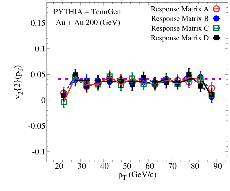
Figure 1: Comparison of the $p_{T}$ dependence of the $v^{\prime}_{2}\{2k\}(p_{T})$ for Au+Au collisions at 200 GeV with several response matrices constructed with different azimuthal distributions of jets. The dashed line represents the true $v^{\prime}_{2}(p_{T})$ values. Response Matrix A, B, and C are constructed with flat constant azimuthal distributions of jets, corresponding to 0.05, 0.1, and 0.2 respectively. Response Matrix D is constructed with a azimuthal distribution that increases linearly with jet $p_{T}$ of jets.

III Results

The simulated data using PYTHIA+TennGen are analyzed using the two- and four-particle cumulant methods with several input flow signals. We present the $v^{\prime}_{n,\text{jet}}\{2\}$ for several $p_{T,jet}$ selection for Au+Au at 200 GeV in Fig. 2. The input $v^{\prime,\text{MC}}_{n,\text{jet}}$ is a constant equal to $0.08$, $0.02$, and $0.01$ for $n=$ 2, 3 and 4, respectively. The $v^{\prime,\text{corr}}_{n,\text{jet}}\{2k\}$ are obtained after five iterations of Bayesian unfolding. Our results reflect the capabilities of using the two-particle cumulant method to reflect the input et $v^{\prime}_{n}$. The presented results also reflected the input sensitivity to the flow harmonic order attenuation.

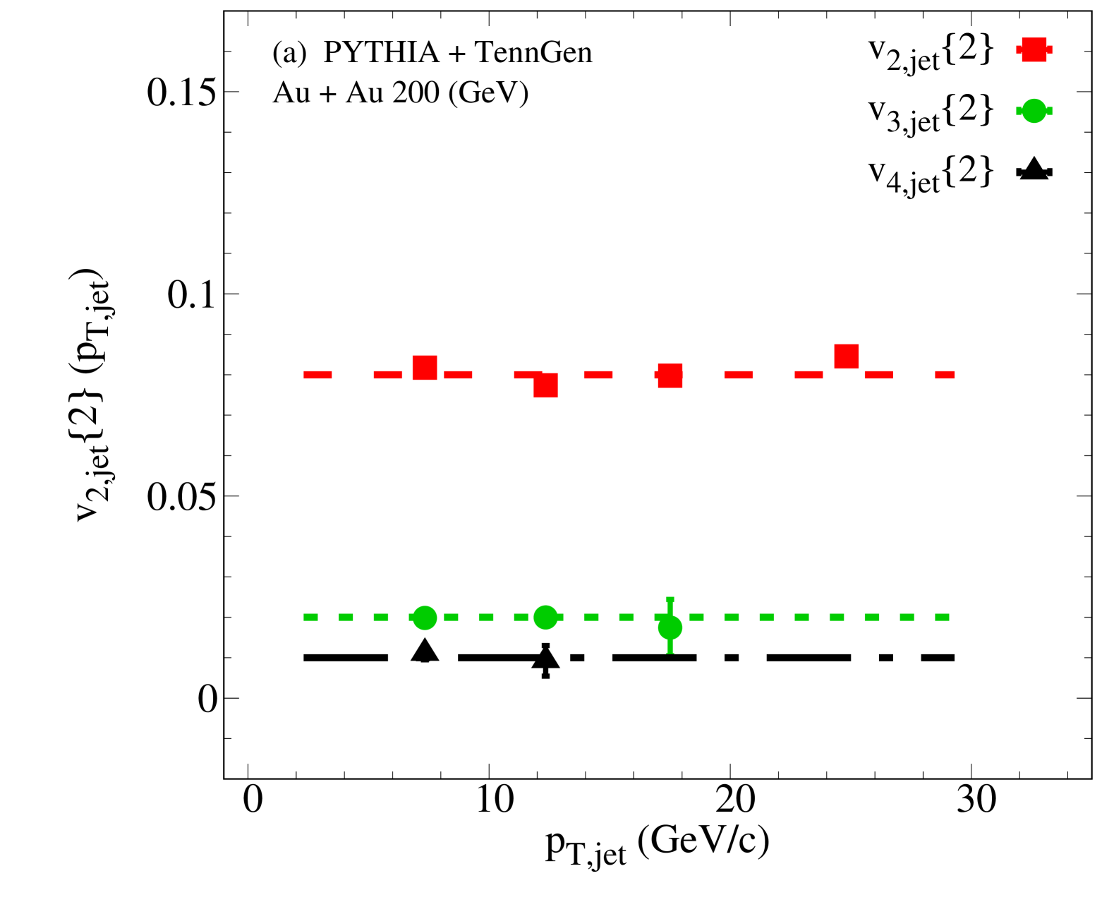
Figure 2: Comparison of the $p_{T}$ dependence of $v^{\prime}_{2,\text{jet}}(p_{T,jet})$, $v^{\prime}_{3,\text{jet}}(p_{T,jet})$, and $v^{\prime}_{4,\text{jet}}(p_{T,jet})$ for Au+Au collisions at 200 GeV. The dashed line represents the true $v^{\prime}_{n,\text{jet}}(p_{T,jet})$ values.

Extending our analysis to the four-particle cumulant will offer deeper insights into the impact of flow fluctuations on jet flow measurements, as well as the effects of short- and long-range correlations. In this context, short-range correlations primarily arise from localized effects, such as particle decays or intra-jet correlations Lacey (2006); Borghini et al. (2000); Luzum and Ollitrault (2011); Retinskaya et al. (2012); Aad et al. (2012). These contributions can be mitigated by applying multi-particle sub-event cumulant methods. Figure 3 presents the corrected $v^{\prime}_{2,\text{jet}}\{2k\}$ (where $k=$ 1 or 2 for the 2- and 4-particle correlation, respectively) as a function of $p_{T,jet}$ for various functional forms of $v^{\prime,\text{MC}}_{n,\text{jet}}$. These forms encompass different realistic scenarios where $v^{\prime}_{n,\text{jet}}$ remains either independent of or gradually increases with $p_{T,jet}$, as well as physically unrealistic forms, such as $v^{\prime}_{n,\text{jet}}\propto\cos(p_{T,jet})$. The inclusion of both realistic and unrealistic models underscores the robustness of our method in reconstructing differential jet azimuthal anisotropies, even under extreme conditions. Furthermore, our results indicate an agreement between $v^{\prime}_{2,\text{jet}}\{2\}$ and $v^{\prime}_{2,\text{jet}}\{4\}$, reflecting the model’s nature, which lacks flow fluctuations effects.

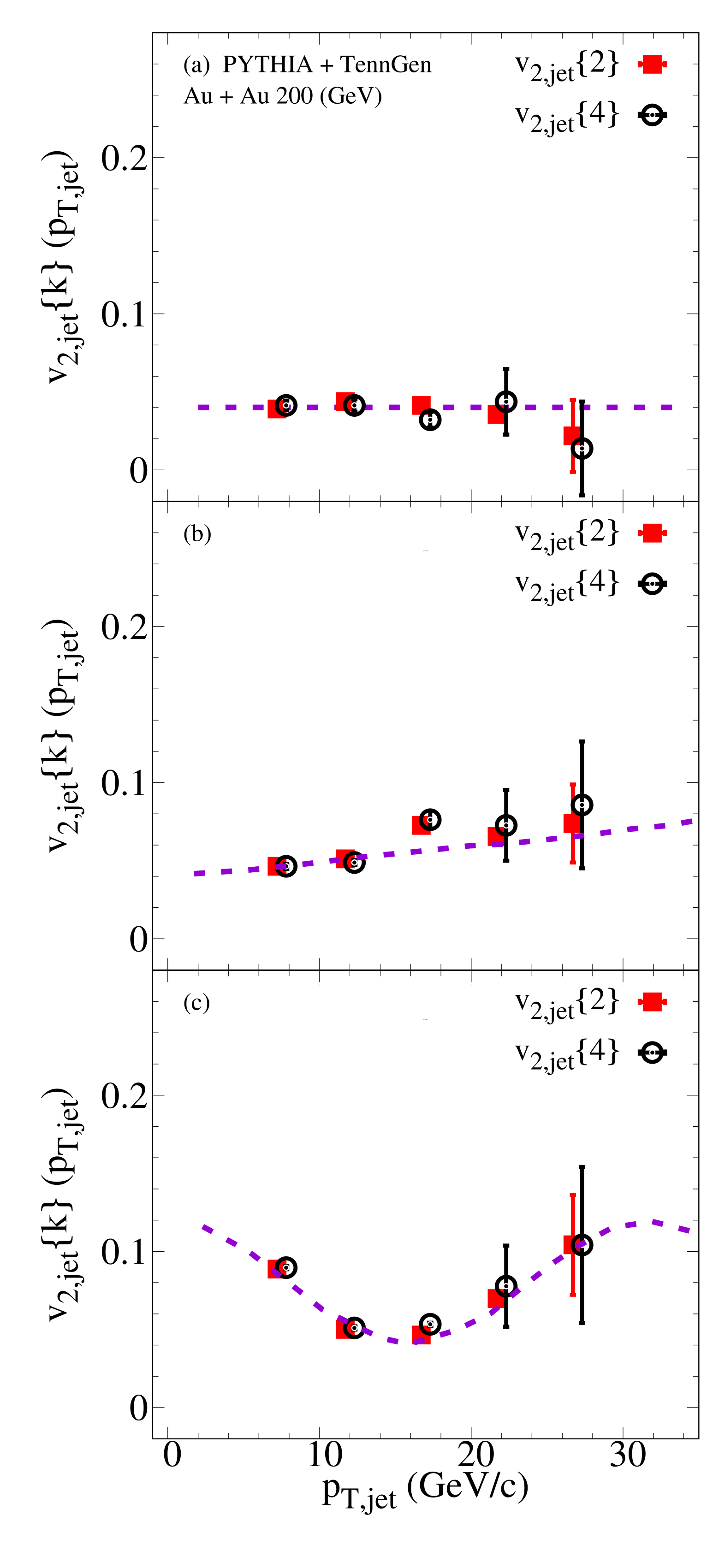
Figure 3: Comparison of the $p_{T}$ dependence of the $v^{\prime}_{2,\text{jet}}\{2k\}(p_{T})$ for Au+Au collisions at 200 GeV. The dashed line represents the true $v^{\prime}_{n,\text{jet}}(p_{T})$ values.

IV Conclusions

This work demonstrates the utility of two- and four-particle cumulant methods for measuring jet anisotropies, leveraging TennGen and PYTHIA models to simulate data representative jet backgrounds in the quark-gluon plasma. Our findings show that cumulants can be used to effectively reconstruct jet azimuthal anisotropies, capturing their flow characteristics and providing a robust means to analyze high-$p_{T}$ jet azimuthal anisotropy. This methodology offers promise for disentangling long and short range correlations between jets. Since it is not possible to reconstruct an event plane in small systems, this technique can be used to advance the understanding of jet interactions and anisotropy in heavy-ion and smaller collision systems.

Appendix A Cumulant method

We use the method presented in Bilandzic et al. (2011) which calculates multi-particle cumulants in terms of moments of of $\mathbf{Q}$ vectors defined as

$$\mathbf{Q}_{n}\equiv\sum_{k=1}^{M}e^{in\phi_{k}}$$ (5)

where $M$ is the multiplicity of the referenced sub-event and $\phi_{k}$ is the azimuthal angle of particles labeled as Reference Flow Particles (RFP). We define our sub-event region away from mid-rapidity $3.1<|\eta|<5.1$ and, for this study, simulate events with $M$ fixed at 363. This $M$ corresponds to an average 20-30$\%$ central Au+Au $\sqrt{s_{NN}}=200$ GeV collision Aamodt et al. (2010). We use a single bracket to denote average moments of Eq. 5 $\langle 2k_{n}\rangle$ which are averaged over all $M$ and double brackets to denote event-averaged moments $\langle\langle(2k)_{n}\rangle\rangle$ which are averaged over all events. Using moments of Eq. 5, the single event $n^{\mathrm{th}}$-order $2$- and $4$-particle reference azimuthal correlations can be expressed as

$$\langle 2_{n}\rangle=\frac{|\mathbf{Q}_{n}|^{2}-M}{M(M-1)}$$ (6)

and

$$\langle 4_{n}\rangle= \frac{|\mathbf{Q}_{n}|^{2}+|\mathbf{Q}_{2n}|^{2}-2\Re\{\mathbf{Q}_{2n}\mathbf{Q}_{n}^{*}\mathbf{Q}_{n}^{*}\}}{M(M-1)(M-2)(M-3)}$$ (7)

$$-2\frac{(M-2)|\mathbf{Q}_{n}|^{2}-M(M-3)}{M(M-1)(M-2)(M-3)}$$

where $|\mathbf{Q}_{n}|^{2}$ is the squared magnitude of $\mathbf{Q}$, $\mathbf{Q}_{2n}$ is the $\mathbf{Q}$-vector for $n=2n$, $\Re\{\cdot\}$ is the real component of the complex argument and $M$ is the reference multiplicity. The event averaged $n^{\mathrm{th}}$-order $2k$-particle reference azimuthal correlation $\langle\langle(2k)_{n}\rangle\rangle$ is computed with a weighted sum of the single event reference azimuthal correlation

$$\langle\langle(2k)_{n}\rangle\rangle=\frac{1}{W\{2k\}}\sum_{i=1}^{N_{\text{events}}}(w\{2k\}){}_{i}(\langle(2k)_{n}\rangle)_{i}$$ (8)

where $(w\{2k\})_{i}$ are event weights and $W\{2k\}$ is the sum of all event weights. Common choices for weights are reference multiplicity or particle momentum. In the case when the multiplicity of the reference is limited methods for momentum weighting are outlined in Bilandzic et al. (2011). In our model, $M$ is fixed and the $v_{n}$ of TennGen is independent of multiplicity leading us to use the weights

$$w\{2\}=M(M-1)$$ (9)

$$w\{4\}=M(M-1)(M-2)(M-3)$$

for $2$- and $4$-particle RFP correlations respectively.

The second order cumulant for the reference sub event is defined as

$$c_{n}\{2\}\equiv\langle\langle 2_{n}\rangle\rangle,$$ (10)

which is simply the event averaged $n^{\mathrm{th}}$-order $2$-particle reference azimuthal correlation defined in Eq. 6. The fourth order reference cumulant is given by

$$c_{n}\{4\}\equiv\langle\langle 4_{n}\rangle\rangle-2\cdot\langle\langle 2_{n}\rangle\rangle^{2}.$$ (11)

which is the $n^{\mathrm{th}}$-order $4$-particle reference azimuthal correlation corrected for event-by-event fluctuations in the $n^{\mathrm{th}}$-order $2$-particle reference azimuthal correlation.

The differential single event azimuthal correlation for jets with respect to the reference correlation is calculated using additional flow vector $\mathbf{p}$, as well as the reference flow vector $\mathbf{Q}$ defined in Eq. 5. To measure the jet $v_{n}$, the Point of Interest (POI) vector $\mathbf{p}$, is built using the azimuthal angle of all jets in an event within $|\eta_{\text{jet}}|<1.1-R$, defined as

$$\mathbf{p}_{n}\equiv\sum_{k=1}^{m_{p}}e^{in\psi_{k}}$$ (12)

where $m_{p}$ is the number of jets within a given $p_{T}$ bin in an event and $\psi_{k}$ is the azimuthal angle of the jet axis.

The $n^{\mathrm{th}}$-order $2$- and $4$-particle differential single event azimuthal correlations are expressed as

$$\langle 2^{\prime}_{n}\rangle=\frac{\mathbf{p}_{n}\mathbf{Q}_{n}^{*}}{m_{p}M}$$ (13)

and

$$\langle 4^{\prime}_{n}\rangle =\frac{(|\mathbf{Q}_{n}|^{2}-2M+2)\mathbf{p}_{n}\mathbf{Q}_{n}^{*}-\mathbf{p}_{n}\mathbf{Q}_{n}\mathbf{Q}_{2n}^{*}}{m_{p}M(M-1)(M-2)}$$ (14)

where $m_{p}$ is the number of jets within a given $p_{T}$ bin in an event, and $\mathbf{p}_{n}$ is the POI vector. The event averaged $n^{\mathrm{th}}$-order $2k$-particle reference differential azimuthal correlation $\langle\langle(2k)^{\prime}_{n}\rangle\rangle$ is computed similar to Eq. 8 with the corresponding weights

$$w^{\prime}\{2\}=m_{p}M$$ (15)

$$w^{\prime}\{4\}=m_{p}M(M-1)(M-2)$$

for the differential $2$- and $4$-particle azimuthal correlations respectively.

These definitions for $\langle 2^{\prime}_{n}\rangle$ and $\langle 4^{\prime}_{n}\rangle$ differ slightly from the standard $n^{\mathrm{th}}$-order $2$- and $4$-particle differential single event azimuthal correlations Bilandzic et al. (2011) due to the fact that we do not have to consider points which are labeled as both RFP and POI because the azimuthal angle of the jet axis $\psi_{\text{jet}}$ is a composite angle from recombination of particles using a jet clustering algorithm. In practice, for jet $v_{n}$, it may be necessary to use RFP and POI correlations in different rapidity regions in order to avoid autocorrelations from using jet constituents in the RFP.

From the definitions for $\langle 2^{\prime}_{n}\rangle$ and $\langle 4^{\prime}_{n}\rangle$, the second and fourth order POI cumulants can be defined as

$$d_{n}\{2\}\equiv\langle\langle 2^{\prime}_{n}\rangle\rangle$$ (16)

and

$$d_{n}\{4\}\equiv\langle\langle 4^{\prime}_{n}\rangle\rangle-2\cdot\langle\langle 2^{\prime}_{n}\rangle\rangle\langle\langle 2_{n}\rangle\rangle$$ (17)

where $d_{n}\{2\}$ is the the $n^{\mathrm{th}}$-order $2$-particle average differential azimuthal correlation and $d_{n}\{4\}$ is the $n^{\mathrm{th}}$-order $4$-particle differential azimuthal correlation corrected for event-by-event fluctuations.

The reference azimuthal anisotropies are calculated from the reference cumulants $c_{n}\{2k\}$ defined in eqs. 10 11

$$v_{n}\{2\}\equiv\sqrt{c_{n}\{2\}}$$ (18)

and

$$v_{n}\{4\}\equiv\sqrt[4]{-c_{n}\{4\}}$$ (19)

where $v_{n}\{2\}$ and $v_{n}\{4\}$ are used to denote estimations of the integrated flow $v_{n}$ using the $2^{\text{nd}}$ and $4^{\text{th}}$-order cumulants respectively.

The differential jet azimuthal anisotropies $v^{\prime}_{n,\text{jet}}\{2k\}$ are calculated using the differential cumulants $d_{n}\{2k\}$ defined in eqs. 16 17 with respect to the the reference azimuthal anisotropies $v_{n}\{2k\}$

$$v^{\prime}_{n,\text{jet}}\{2\}(p_{T,jet})=\frac{d_{n}\{2\}(p_{T,jet})}{v_{n}\{2\}}$$ (20)

$$v^{\prime}_{n,\text{jet}}\{2\}(p_{T,jet})=-\frac{d_{n}\{4\}(p_{T,jet})}{(v_{n}\{4\})^{3/4}}$$ (21)

where $v^{\prime}_{n,\text{jet}}\{2\}(p_{T,jet})$ and $v^{\prime}_{n,\text{jet}}\{4\}(p_{T,jet})$ are used to denote estimations of the differential flow for jets with a given transverse momentum $p_{T,jet}$ using the $2^{\text{nd}}$ and $4^{\text{th}}$-order differential cumulants respectively.

References

- Adams et al. (2005) J. Adams et al. (STAR), Nucl. Phys. A 757, 102 (2005), arXiv:nucl-ex/0501009 .
- Adcox et al. (2005) K. Adcox et al. (PHENIX), Nucl. Phys. A 757, 184 (2005), arXiv:nucl-ex/0410003 .
- Arsene et al. (2005) I. Arsene et al. (BRAHMS), Nucl. Phys. A 757, 1 (2005), arXiv:nucl-ex/0410020 .
- Back et al. (2005) B. B. Back et al. (PHOBOS), Nucl. Phys. A 757, 28 (2005), arXiv:nucl-ex/0410022 .
- Acharya et al. (2024) S. Acharya et al. (ALICE), Eur. Phys. J. C 84, 813 (2024), arXiv:2211.04384 [nucl-ex] .
- Hayrapetyan et al. (2024) A. Hayrapetyan et al. (CMS), ” ” (2024), arXiv:2405.10785 [nucl-ex] .
- Busza et al. (2018) W. Busza, K. Rajagopal, and W. van der Schee, Ann. Rev. Nucl. Part. Sci. 68, 339 (2018), arXiv:1802.04801 [hep-ph] .
- Hirano et al. (2006) T. Hirano, U. W. Heinz, D. Kharzeev, R. Lacey, and Y. Nara, Phys. Lett. B 636, 299 (2006), arXiv:nucl-th/0511046 .
- Huovinen et al. (2001) P. Huovinen, P. F. Kolb, U. W. Heinz, P. V. Ruuskanen, and S. A. Voloshin, Phys. Lett. B 503, 58 (2001), arXiv:hep-ph/0101136 .
- Hirano and Tsuda (2002) T. Hirano and K. Tsuda, Phys. Rev. C 66, 054905 (2002), arXiv:nucl-th/0205043 .
- Romatschke and Romatschke (2007) P. Romatschke and U. Romatschke, Phys. Rev. Lett. 99, 172301 (2007), arXiv:0706.1522 [nucl-th] .
- Song et al. (2011) H. Song, S. A. Bass, U. Heinz, T. Hirano, and C. Shen, Phys. Rev. Lett. 106, 192301 (2011), [Erratum: Phys.Rev.Lett. 109, 139904 (2012)], arXiv:1011.2783 [nucl-th] .
- Schenke et al. (2011) B. Schenke, S. Jeon, and C. Gale, Phys. Lett. B 702, 59 (2011), arXiv:1102.0575 [hep-ph] .
- Lacey et al. (2016) R. A. Lacey, D. Reynolds, A. Taranenko, N. N. Ajitanand, J. M. Alexander, F.-H. Liu, Y. Gu, and A. Mwai, J. Phys. G 43, 10LT01 (2016), arXiv:1311.1728 [nucl-ex] .
- Voloshin and Zhang (1996) S. Voloshin and Y. Zhang, Z. Phys. C 70, 665 (1996), arXiv:hep-ph/9407282 .
- Poskanzer and Voloshin (1998) A. M. Poskanzer and S. A. Voloshin, Phys. Rev. C 58, 1671 (1998), arXiv:nucl-ex/9805001 .
- Connors et al. (2018) M. Connors, C. Nattrass, R. Reed, and S. Salur, Rev. Mod. Phys. 90, 025005 (2018), arXiv:1705.01974 [nucl-ex] .
- Qin and Wang (2015) G.-Y. Qin and X.-N. Wang, Int. J. Mod. Phys. E 24, 1530014 (2015), arXiv:1511.00790 [hep-ph] .
- Mehtar-Tani et al. (2013) Y. Mehtar-Tani, J. G. Milhano, and K. Tywoniuk, Int. J. Mod. Phys. A 28, 1340013 (2013), arXiv:1302.2579 [hep-ph] .
- Blaizot and Mehtar-Tani (2015) J.-P. Blaizot and Y. Mehtar-Tani, Int. J. Mod. Phys. E 24, 1530012 (2015), arXiv:1503.05958 [hep-ph] .
- Sirunyan et al. (2018) A. M. Sirunyan et al. (CMS), Phys. Lett. B 776, 195 (2018), arXiv:1702.00630 [hep-ex] .
- Aad et al. (2013a) G. Aad et al. (ATLAS), Phys. Rev. Lett. 111, 152301 (2013a), arXiv:1306.6469 [hep-ex] .
- Acharya et al. (2018) S. Acharya et al. (ALICE), JHEP 07, 103 (2018), arXiv:1804.02944 [nucl-ex] .
- Gyulassy et al. (2001) M. Gyulassy, I. Vitev, and X. N. Wang, Phys. Rev. Lett. 86, 2537 (2001), arXiv:nucl-th/0012092 .
- Shuryak (2002) E. V. Shuryak, Phys. Rev. C 66, 027902 (2002), arXiv:nucl-th/0112042 .
- Jia (2013) J. Jia, Phys. Rev. C 87, 061901 (2013), arXiv:1203.3265 [nucl-th] .
- Molnar and Sun (2013) D. Molnar and D. Sun, ” ” (2013), arXiv:1305.1046 [nucl-th] .
- Noronha-Hostler et al. (2016) J. Noronha-Hostler, B. Betz, J. Noronha, and M. Gyulassy, Phys. Rev. Lett. 116, 252301 (2016), arXiv:1602.03788 [nucl-th] .
- Betz et al. (2017) B. Betz, M. Gyulassy, M. Luzum, J. Noronha, J. Noronha-Hostler, I. Portillo, and C. Ratti, Phys. Rev. C 95, 044901 (2017), arXiv:1609.05171 [nucl-th] .
- Holtermann et al. (2024) A. Holtermann, J. Noronha-Hostler, A. M. Sickles, and X. Wang, (2024), arXiv:2402.03512 [hep-ph] .
- Barreto et al. (2022) L. Barreto, F. M. Canedo, M. G. Munhoz, J. Noronha, and J. Noronha-Hostler, ” ” (2022), arXiv:2208.02061 [nucl-th] .
- Zhang and Liao (2013) X. Zhang and J. Liao, ” ” (2013), arXiv:1311.5463 [nucl-th] .
- Adam et al. (2016a) J. Adam et al. (ALICE), Phys. Lett. B 753, 511 (2016a), arXiv:1509.07334 [nucl-ex] .
- Andres et al. (2020) C. Andres, N. Armesto, H. Niemi, R. Paatelainen, and C. A. Salgado, Phys. Lett. B 803, 135318 (2020), arXiv:1902.03231 [hep-ph] .
- Zigic et al. (2022a) D. Zigic, J. Auvinen, I. Salom, M. Djordjevic, and P. Huovinen, Phys. Rev. C 106, 044909 (2022a), arXiv:2208.09886 [hep-ph] .
- Zigic et al. (2022b) D. Zigic, I. Salom, J. Auvinen, P. Huovinen, and M. Djordjevic, Front. in Phys. 10, 957019 (2022b), arXiv:2110.01544 [nucl-th] .
- Aad et al. (2022) G. Aad et al. (ATLAS), Phys. Rev. C 105, 064903 (2022), arXiv:2111.06606 [nucl-ex] .
- Aad et al. (2013b) G. Aad et al. (ATLAS), Phys. Rev. Lett. 110, 182302 (2013b), arXiv:1212.5198 [hep-ex] .
- Khachatryan et al. (2010) V. Khachatryan et al. (CMS), JHEP 09, 091 (2010), arXiv:1009.4122 [hep-ex] .
- Khachatryan et al. (2015) V. Khachatryan et al. (CMS), Phys. Rev. Lett. 115, 012301 (2015), arXiv:1502.05382 [nucl-ex] .
- Abelev et al. (2013a) B. B. Abelev et al. (ALICE), Phys. Lett. B 727, 371 (2013a), arXiv:1307.1094 [nucl-ex] .
- Aidala et al. (2019) C. Aidala et al. (PHENIX), Nature Phys. 15, 214 (2019), arXiv:1805.02973 [nucl-ex] .
- Abdulhamid et al. (2023) M. I. Abdulhamid et al. (STAR), Phys. Rev. Lett. 130, 242301 (2023), arXiv:2210.11352 [nucl-ex] .
- Adare et al. (2016a) A. Adare et al. (PHENIX), Phys. Rev. Lett. 116, 122301 (2016a), arXiv:1509.04657 [nucl-ex] .
- Acharya et al. (2020) U. Acharya et al. (PHENIX), Phys. Rev. C 102, 054910 (2020), arXiv:2005.14270 [hep-ex] .
- Abdulameer et al. (2025) N. J. Abdulameer et al. (PHENIX), Phys. Rev. Lett. 134, 022302 (2025), arXiv:2303.12899 [nucl-ex] .
- Aad et al. (2023) G. Aad et al. (ATLAS), Phys. Rev. Lett. 131, 072301 (2023), arXiv:2206.01138 [nucl-ex] .
- Abdallah et al. (2022) M. Abdallah et al. (STAR), Phys. Rev. C 105, 014901 (2022), arXiv:2109.00131 [nucl-ex] .
- Hughes et al. (2022) C. Hughes, A. C. Oliveira Da Silva, and C. Nattrass, Phys. Rev. C 106, 044915 (2022), arXiv:2005.02320 [hep-ph] .
- Mengel et al. (2023) T. Mengel, P. Steffanic, C. Hughes, A. C. O. da Silva, and C. Nattrass, Phys. Rev. C 108, L021901 (2023), arXiv:2303.08275 [hep-ex] .
- Hughes and Mengel (2019) C. Hughes and T. Mengel, “Github: TennGen,” (2019).
- Sjostrand et al. (2006) T. Sjostrand, S. Mrenna, and P. Z. Skands, JHEP 05, 026 (2006), arXiv:hep-ph/0603175 [hep-ph] .
- Sjostrand et al. (2008) T. Sjostrand, S. Mrenna, and P. Z. Skands, Comput. Phys. Commun. 178, 852 (2008), arXiv:0710.3820 [hep-ph] .
- Mengel and Hughes (2022) T. Mengel and C. Hughes, “Github: tenngen200,” (2022).
- Aamodt et al. (2010) K. Aamodt et al. (ALICE Collaboration), Phys. Rev. Lett. 106, 032301. 14 p (2010).
- Abelev et al. (2013b) B. Abelev et al. (ALICE), Phys. Rev. C88, 044910 (2013b), arXiv:1303.0737 [hep-ex] .
- Ristea et al. (2013) O. Ristea, A. Jipa, C. Ristea, T. Esanu, M. Calin, A. Barzu, A. Scurtu, and I. Abu-Quoad, Proceedings, 11th International Conference on Nucleus-Nucleus Collisions (NN2012): San Antonio, Texas, May 27-June 1, 2012, J. Phys. Conf. Ser. 420, 012041 (2013).
- Schnedermann et al. (1993) E. Schnedermann, J. Sollfrank, and U. W. Heinz, Phys. Rev. C 48, 2462 (1993), arXiv:nucl-th/9307020 .
- Adare et al. (2016b) A. Adare et al. (PHENIX), Phys. Rev. C 93, 051902 (2016b), arXiv:1412.1038 [nucl-ex] .
- Adam et al. (2016b) J. Adam et al. (ALICE), JHEP 09, 164 (2016b), arXiv:1606.06057 [nucl-ex] .
- Skands et al. (2014) P. Skands, S. Carrazza, and J. Rojo, Eur. Phys. J. C 74, 3024 (2014), arXiv:1404.5630 [hep-ph] .
- Cacciari et al. (2012) M. Cacciari, G. P. Salam, and G. Soyez, Eur. Phys. J. C 72, 1896 (2012), arXiv:1111.6097 [hep-ph] .
- Steffanic et al. (2023) P. Steffanic, C. Hughes, and C. Nattrass, Phys. Rev. C 108, 024909 (2023), arXiv:2301.09148 [hep-ph] .
- Bilandzic et al. (2011) A. Bilandzic, R. Snellings, and S. Voloshin, Phys. Rev. C 83, 044913 (2011), arXiv:1010.0233 [nucl-ex] .
- Jia et al. (2017) J. Jia, M. Zhou, and A. Trzupek, Phys. Rev. C 96, 034906 (2017), arXiv:1701.03830 [nucl-th] .
- D’Agostini (1995) G. D’Agostini, Nuclear Instruments and Methods in Physics Research Section A: Accelerators, Spectrometers, Detectors and Associated Equipment 362, 487 (1995).
- Brenner et al. (2020) L. Brenner, R. Balasubramanian, C. Burgard, W. Verkerke, G. Cowan, P. Verschuuren, and V. Croft, Int. J. Mod. Phys. A 35, 2050145 (2020), arXiv:1910.14654 [physics.data-an] .
- Lacey (2006) R. A. Lacey, Proceedings, 18th International Conference on Ultra-Relativistic Nucleus-Nucleus Collisions (Quark Matter 2005): Budapest, Hungary, August 4-9, 2005, Nucl. Phys. A774, 199 (2006), arXiv:nucl-ex/0510029 [nucl-ex] .
- Borghini et al. (2000) N. Borghini, P. M. Dinh, and J.-Y. Ollitrault, Phys. Rev. C62, 034902 (2000), arXiv:nucl-th/0004026 [nucl-th] .
- Luzum and Ollitrault (2011) M. Luzum and J.-Y. Ollitrault, Phys. Rev. Lett. 106, 102301 (2011), arXiv:1011.6361 [nucl-ex] .
- Retinskaya et al. (2012) E. Retinskaya, M. Luzum, and J.-Y. Ollitrault, Phys. Rev. Lett. 108, 252302 (2012), arXiv:1203.0931 [nucl-th] .
- Aad et al. (2012) G. Aad et al. (ATLAS), Phys. Rev. C86, 014907 (2012), arXiv:1203.3087 [hep-ex] .