Fault Localization and State Estimation of Power Grid under Parallel Cyber-Physical Attacks

Abstract

Parallel cyber-physical attacks (PCPA) refer to those attacks on power grids by disturbing/cutting off physical transmission lines and meanwhile blocking transmission of measurement data to dwarf or delay the system protection and recovery actions. Such fierce hostile attacks impose critical threats to the modern power grids when there is a fusion of power grids and telecommunication technologies. In this paper, we investigate the fault diagnosis problem of faulty transmission lines under a broader spectrum of PCPA for a linearized (or DC) power flow model. The physical attack mechanism of PCPA includes not only disconnection but also admittance value modification on transmission lines, for example, by invading distributed flexible AC transmission system (D-FACTS). To tackle the problem, we first recover the information of voltage phase angles within the attacked area. Using the information of voltage phase angle and power injection of buses, a graph attention network-based fault localization (GAT-FL) algorithm is proposed to find the locations of the physical attacks. By capitalizing on the feature extraction capability of the GAT on graph data, the fault localization algorithm outperforms the existing results when under cyber attacks, e.g., denial of service (DoS) attacks. A line state identification algorithm is then developed to identify the states of the transmission lines within the attacked area. Specifically, the algorithm restores the power injection of buses within the attacked area and then identities the state of all the transmission lines within the attacked area by solving a linear programming (LP) problem. Experimental simulations are conducted on IEEE 30/118 bus standard test cases to demonstrate the effectiveness of the proposed fault diagnosis algorithms.

I Introduction

In recent years, smart grids [1] have experienced rapid developments, driven by the the needs for more effective control of power systems and more efficient utilization of renewable and non-renewable energy resources. Modern smart grids require the deployment of a large number of smart devices, such as smart meters. Remote Terminal Units (RTUs) and Phasor Measurement Units (PMUs) are the primary smart meters that acquire physical measurements and transmit the measured signals to Supervisory Control and Data Acquisition Systems (SCADAs). SCADAs estimate the state of the systems [2], analyze potential dangers [3], and make decisions [4] based on the received information to maintain stable operation and cyber-physical security of power grids. Compared to traditional power grids, such changes indicate a big step towards operating power systems more efficiently and effectively.

The plausible evolution brings along great benefits and potentials to future power systems, and new threats and challenges as well. The most critical challenges, arguably, may be those on the system security and safety imposed by some most sophisticated hostile cyber attacks [5, 6]. Extensive studies have been mainly focusing on typical cyber attacks that aim to degrade or even paralyze system manager’s capability of situation awareness, e.g., by carrying out DoS attacks [7]. More sophisticated attacks include false data injection (FDI) attacks which try to inject false information of system state without triggering any alarm at the control center [8, 9]. To address such challenges, moving target defense (MTD) mechanism has been proposed (e.g., [10]). This mechanism enables system operators to proactively alter branch susceptances using D-Facts, thereby disrupting the adversary’s knowledge of the power grid and failing the FDI attacks. Despite the reservations of some scholars about the side effects of MTD on system stability, MTD is able to cope well with cyber-attacks in most cases [11, 12, 13].

Another form of hostile attacks on cyber-physical power systems, potentially more damaging and dangerous than FDI attacks, involves simultaneous assaults on both cyber and physical systems. The severity of these cyber-physical attacks is typically manifested in rendering the operators’ knowledge of the power system obsolete and impairing/deceiving sensors of the power system to prevent operators from implementing timely countermeasures (e.g., [14, 15]).

To date, studies in this field have progressed in two main directions. One type of cyber-physical attacks is known as coordinated cyber-physical attacks (CCPA) [16]. In CCPA, physical attacks aim to change the topological structure of the graph by destroying generators, transmission lines, or transformers, while cyber attacks, typically FDI attacks, are launched simultaneously to hide physical attack actions until leading to severe devastation [17]. In [16], defense solutions against CCPA were presented using measurements from a limited number of secured meters and online tracking of the equivalent impedance. To detect CCPA for a discrete-time time-varying power system at a relatively low computation complexity, an attack detector was designed based on exponentially weighted moving average statistic, standardization of decision statistics and MTD [18]. In [19], Chen et al. proposed a defense algorithm which combines MTD with machine learning methods to counter CCPA for a DC power flow model while significantly lowering the model dependence. It is noted that CCPA is a specific type stealthy attack which requires neat design, based on rather comprehensive knowledge of system, to hide the physical attacks from measurements for a sufficiently long period of time. There is another type of cyber-physical attack, named joint cyber-physical attacks (JCPA), proposed in [20]. The significant difference between JCPA and CCPA is that, in JCPA, the cyber attacks are to block the measurement data transmission from the attacked area rather than hiding the existence of attack, and hence may not necessarily request excessive knowledge of system. In [20], an LP algorithm was presented to locate the faults caused by JCPA under certain conditions (that the network topology is well-supported after the attack). The authors later further extended their results for scenarios involving measurement noise and uncertainties [21]. For both of these two results, however, it is assumed that no cycle exists within the attacked area. Further, an iterative estimation algorithm based on a linear minimum mean square error (MMSE) estimation was developed in [22] to locate failures under JCPA. Compared to other types of attacks, JCPA are more concentrated and regional, which may pose greater pressure on fault localization. Besides, it is noted that JCPA may lead to an islanding problem, which may cause unknown changes in the power injection of the attacked area. Without good knowledge of power injection, failure localization becomes rather challenging. To address this problem, for the cases where there exist cycles in the attacked area, Huang et al. presented a defense method adopting an LP algorithm and a voting verification algorithm. The voting verification algorithm is capable of verifying the fault locations derived from the LP algorithm in polynomial time [23].

In existing studies on CCPA and JCPA, it has been assumed that the physical attacks involve only cutting transmission lines. Algorithm designs for failure localization have all been based on this assumption. However, physical attacks are not limited to link cutting. For example, changes of temperature may cause the changes of branch admittance. In fact, as pointed out in [24], the worst attacks that can cause most serious damages to power systems, in most cases, are not link cut but altering the admittance of transmission lines to certain specific values. Therefore, it is necessary to consider the more general cases of attacks by admittance altering in order to better protect the systems against cyber-physical attacks. To differentiate the cases under general attacks of admittance altering from link cutting that have been considered in JCPA and CCPA, we term such cases as being under parallel cyber-physical attacks (PCPA). Obviously, PCPA includes JCPA as one of its special cases. In addition, different from the studies in [20, 21, 22, 23], we consider the case possibly with multiple cycles existing within the attacked area, while it is still assumed that measurement data transmission from the attacked area is completely blocked. Introducing such changes poses a significant challenge to fault localization and state identification, thus precluding the direct applications of the faults diagnosis methods developed for JCPA and CCPA. A new and robust method for countering PCPA is needed.

In this study, we design a defense mechanism for fault diagnosis under PCPA based on a simplified, linearized AC (or DC) power flow model. Our main contributions are twofold:

• We propose a graph attention network-based fault localization (GAT-FL) algorithm to estimate the likelihood that physical attacks occur on each of the transmission lines within the attacked area. Utilizing the capability of the GAT to extract high-level feature from graph data, the proposed algorithm could efficiently locate faults in the attacked area.

• Motivated by existing work [20, 23], we formulate the line state identification (LSI) problem under PCPA as an LP problem and then propose an LP-based LSI algorithm. In this algorithm, a parameter vector is extracted from the output of the GAT-FL algorithm and then introduced into the designing of the objective function of LP to ensure the accuracy and computational efficiency of the proposed algorithm.

It may be worth mentioning that our approach is fundamentally different from that proposed in [23]. In [23], based on the assumption that physical attacks are always link cuts, an LP problem was solved with the objective of minimizing the number of faulty transmission lines (known as “sparsity assumption”, as physical link cuts typically do not happen to a large number of transmission lines simultaneously), then a voting algorithm is adopted to verify each possible solution. In our work, the assumption of only having the link cuts does not apply. Instead, we leverage the ability of GAT to extract information from graphs to estimate the most likely locations of faults. For LSI, the proposed LSI algorithm incorporates the output of the GAT-FL algorithm. Such an approach biases the algorithm to focus more effectively on the most likely locations of physical attacks. Compared to existing approaches, the proposed LSI algorithm exhibits greater robustness and effectiveness in more general cases, particularly in scenarios where attacks deviate from the “sparsity assumption”.

Table I summarizes various notations and abbreviations. The rest of the paper is organized as follows. Section II discusses basic graph theory related to the power flow model and formulates the problem under PCPA. Section III provides the detailed theoretical analysis for fault localization under PCPA. Section IV describes the fault diagnosis scheme, including the GAT-FL algorithm and the LSI algorithm. In Section V, we validate the effectiveness of the fault diagnosis framework through numerical experiments. Finally, Section VI concludes this work and points out some future research directions.

TABLE I: Notations and Abbreviations

Notation	Description
$\vec{(\cdot)}$	The vector while $\cdot$ represents any lowercase letters
$\operatorname{supp}(\cdot)$	The set of indices of non-zero entries in a vector
$[\vec{\cdot}]$	The diagonalization of vector $\vec{\cdot}$
$|\cdot|$	The number of the elements in set $\cdot$
$\Gamma$	The diagonal matrix $[\frac{1}{r_{uv}}]_{\{u,v\}\in\cal E}$ ($r_{uv}$: reactance of line $\{u,v\}$)
$I$	The identity matrix with compatible dimension
$\odot$	The Hadamard product
$\|$	The concatenation operation
0 or 1	The vector with all elements $0$ or $1$

II Problem Formulation

II-A Power grid model

In this paper, we investigate a linearized (or DC) power flow model which is a simplified form of the non-linear AC power flow model. The power grid is characterized by the undircted graph $\cal{G}=\left(V,E\right)$, where ${\cal V}=\{1,2,3,...,n\}$ and ${\cal E}=\{e_{1},e_{2},...,e_{m}\}$ are the sets of nodes and edges corresponding to the buses and transmission lines, respectively. For each transmission line $e_{i}$ connecting a pair of buses $\{u,v\}$, the reactance of $e_{i}$ is denoted as $r_{uv}$ (the same as $r_{vu}$). By arbitrarily designating a direction for each line, the topology of $\cal G$ can be represented by the incidence matrix ${\cal D}\in\{-1,0,1\}^{|{\cal V}|\times|{\cal E}|}$, of which the $(i,j)$-th element is defined as:

$${\cal D}_{ij}=\begin{dcases}1&\text{if line $e_{j}$ starts from bus $v_{i}$},\\ -1&\text{if line $e_{j}$ ends at bus $v_{i}$},\\ 0&\text{otherwise}.\end{dcases}$$ (1)

According to [20], it is known that, given the power supply/demand vector $\vec{p}\in\mathbb{R}^{|{\cal V}|}$ and the reactance values, a power flow is a solution $P\in\mathbb{R}^{|{\cal V}|\times|{\cal V}|}$ and $\vec{\theta}\in\mathbb{R}^{|{\cal V}|}$ of :

$$\sum_{v\in{\cal N}_{u}}{p_{uv}}=p_{u},\forall u\in{\cal V}$$ (2a)

$${\theta}_{u}-{\theta}_{v}-r_{uv}p_{uv}=0,\forall\{u,v\}\in{\cal E}$$ (2b)

where ${\cal N}_{u}$ is the set of neighbors of bus $u$, $p_{uv}$ is the power flow from bus $u$ to bus $v$, and $\theta_{u}$ is the voltage phase angles of bus $u$. In the calculation of power flow, the uniqueness of the solution for Eqs. (2a) and (2b) is guaranteed if the demand and the supply are balanced for each bus in a connected graph. Hence, within the entire power network, the relationship between the voltage phase angles $\vec{\theta}$ and the active power injection $\vec{p}$ is delineated as follows:

$$A\vec{\theta}=\vec{p}$$ (3)

where $A\in\mathbb{R}^{|{\cal V}|\times|{\cal V|}}$ is the admittance matrix of $\cal G$, defined as:

$$A_{uv}=\begin{dcases}0,&\text{if}\ u\neq v\ \text{and}\ \{u,v\}\notin{\cal E},\\ -1/r_{uv},&\text{if}\ u\neq v\ \text{and}\ \{u,v\}\in{\cal E},\\ -\sum_{w\in{\cal N}_{u}}{a_{uw}},&\text{if}\ u=v.\end{dcases}$$ (4)

II-B Control system

In a power grid, the SCADA system, as described in [23], can be simplified as the control center.

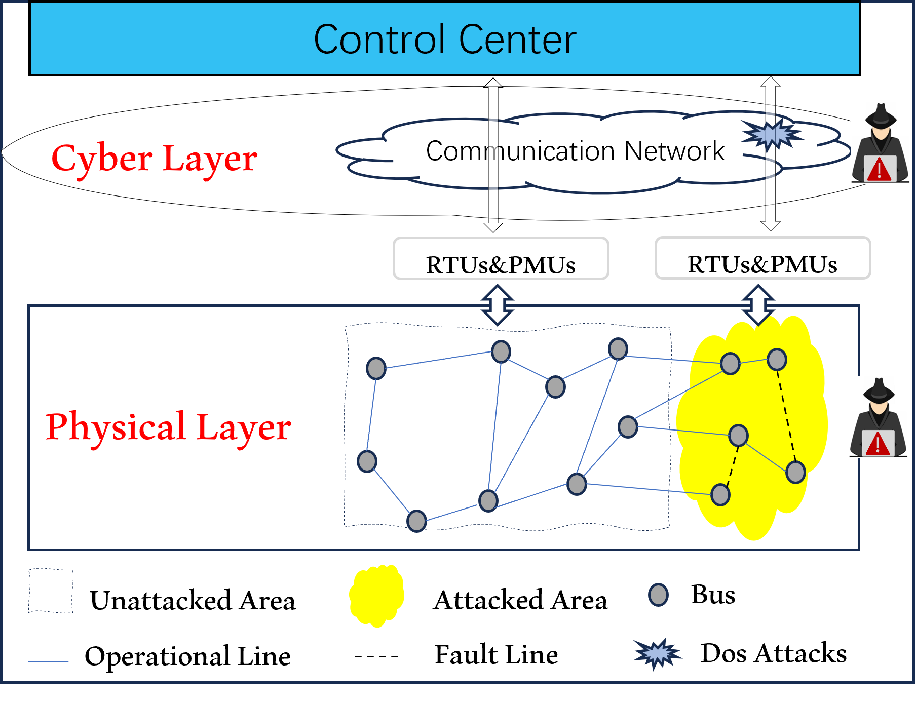
Figure 1: Architecture of power grid and attack scheme of PCPA

For sensor equipments, we assume that each bus is installed with a hybrid sensor deployment of an RTU and a PMU. With such sensor deployment, control center has access to the voltage phase angle and power injection information for each node. All the sensors work to upload measurements of the corresponding buses to the control center through communication network in the cyber layer. The control center shall monitor the states of power grid and make decisions based on these measurements.

II-C Attack model of PCPA

In this study, a model of simultaneous attacks on both the cyber and physical layers is considered. Specifically, on the physical layer, the adversary’s goal is to compromise certain transmission lines in the targeted area of the power grid, resulting in the admittance altering or line disconnections. On the cyber layer, the adversary employs various methods, including severing specific communications or executing DoS attacks on servers, to obstruct the transmission of measurement data from RTUs and PMUs within the attacked area to the control center. A successful PCPA can disrupt the stable operation of the power grid and hinder the localization of physical attacks. It is essential to highlight that PCPA can alter power injections on buses due to the islanding effect. The difficulty of fault diagnosis for PCPA lies in the diversity of attack mechanisms, which are not restricted to link cut. This expansion of attacking capabilities, combined with cyber (DoS) attacks, threaten to drastically weaken the resilience of power systems. PCPA poses significant challenges to system monitoring and stable operation. It necessitates the control center the capabilities of robust failure localization and state identification, especially when measurements are partially compromised.

It is assumed that after an attack the entire power gird still operates steadily without disastrous cascading buses collapse. The attacked area is indicated by $H$ and the rest part of the power grid by $\bar{H}={\cal G}{\setminus}H$. Without loss of generality, it is assumed that ${\cal V}_{H}=\{1,2,3,...,|{\cal V}|_{H}\}$ and ${\cal E}_{H}=\{e_{1},e_{2},...,e_{|{\cal E}_{H}|}\}$. Therefore, for the graph $\cal G$ and its subgraphs $H$ and $\bar{H}$, $A_{H|\cal G}$ denotes the submatrix of$A$ with rows from ${\cal V}_{H}$, and $A_{\bar{H}|\bar{H}}$ denotes the submatrix of $A$ with rows from ${\cal V}_{H}$ and columns from ${\cal V}_{\bar{H}}$. For instance,

$$A=\begin{bmatrix}A_{H|\cal{G}}\\ A_{\bar{H}|\cal{G}}\end{bmatrix}=\begin{bmatrix}A_{H|H}&A_{H|\bar{H}}\\ A_{\bar{H}|H}&A_{\bar{H}|\bar{H}}\end{bmatrix}.$$

The values representing post-attack measurements are denoted by a prime $(^{\prime})$. For example, $\vec{\theta}^{\prime}$ represents the voltage phase angles of the post-attack buses.

In the next section, we provide the theoretical analysis to guide the design of fault localization algorithm under PCPA.

III Analysis on Localization of Faulty Lines under PCPA

In this section, the condition of power systems under PCPA is analyzed from the defense perspective. Specifically, we analyze the system state within the $H$ area based on observed information, which provides theoretical guidelines for designing the fault localization algorithm as well.

III-A Restoration of unknown voltage phase angles

The primary objective of this subsection is to recover post-attack information within the attacked area utilizing the known measurement data from the unaffected area, thus facilitating the localization of the faulty transmission lines.

In this work, the change in supply/demand is taken into account (as some buses may be disconnected after attacks). Define $\vec{\Delta}=\vec{p}-\vec{p}^{\prime}$ as the supply/demand changes resulted from the physical attacks and $F=\{e_{i}\}\subseteq{\cal E}_{H}$ as the set of attacked transmission lines. It is known that $A={\cal D}\Gamma{\cal D}^{T}$ and the post-attack admittance is therefore derived as $A^{\prime}=A-{\cal D}\Gamma[\vec{x}]{\cal D}^{T}$, where $\vec{x}$ is an attacking vector such that $\vec{x}_{e}\in(0,1]$ if and only if $e\in F$. Therefore, we obtain

$$\vec{\Delta}= A\vec{\theta}-A^{\prime}\vec{\theta^{\prime}}$$ (5)

$$= A(\vec{\theta}-\vec{\theta^{\prime}})+{\cal D}\Gamma[\vec{x}]{\cal D}^{T}\vec{\theta}^{\prime}.$$

Apparently, $\vec{\Delta}$ can be partitioned into $\vec{\Delta}_{\bar{H}}$ and $\vec{\Delta}_{H}$. Therefore, for the attacked area $H$, we obtain $\vec{\Delta}_{H}$ according to Eq. (5):

$$\begin{bmatrix}\vec{\Delta}_{H}\\ \vec{\Delta}_{\bar{H}}\end{bmatrix}= \begin{bmatrix}A_{H|\cal{G}}\\ A_{\bar{H}|\cal{G}}\end{bmatrix}(\vec{\theta}-\vec{\theta^{\prime}})+\begin{bmatrix}D^{\prime}_{H|\cal{G}}\\ D^{\prime}_{\bar{H}|\cal{G}}\end{bmatrix}\vec{x}$$ (6)

$$\begin{bmatrix}\vec{\Delta}_{H}\\ \vec{\Delta}_{\bar{H}}\end{bmatrix}= \begin{bmatrix}A_{H|\cal{G}}\\ A_{\bar{H}|\cal{G}}\end{bmatrix}(\vec{\theta}-\vec{\theta^{\prime}})+\begin{bmatrix}D^{\prime}_{H}\vec{x}_{H}\\ \textbf{0}\end{bmatrix},$$

where ${\cal D}^{\prime}={\cal D}\Gamma[{\cal D}^{T}\vec{\theta}^{\prime}]$ and ${\cal D}^{\prime}_{H}$ represents the submatrix of $\cal{D}^{\prime}$ with rows from ${\cal V}_{H}$ and columns from ${\cal E}_{H}$. Inspired by the work of Soltan et al. [20], we have the following lemma.

Lemma 1.

$\operatorname{supp}(A(\vec{\theta}-\vec{\theta}^{\prime})-\vec{\Delta})\subseteq{\cal V}_{H}$.

Proof.

From Eq. (5) and [Lemma 1, [20]], it is easy to have the following equation:

$$A\vec{\theta}-A^{\prime}\vec{\theta}^{\prime}=\vec{\Delta}$$ (7)

$$\Rightarrow\operatorname{supp}(A(\vec{\theta}-\vec{\theta}^{\prime})-\vec{\Delta})\subseteq\bigcup_{e_{i}\in F}e_{i}\subseteq{\cal V}_{H}.$$

For more details, please refer to [20]. ∎

Before restoring the voltage phase angles, let us introduce the assumption to restrict the range of the attacked area, thereby ensuring that the problem is solvable.

Assumption 1.

Assume that $|{\cal V}_{H}|\leq|{\cal V}_{\bar{H}}|$ and $|{\cal E}_{H}|\leq|{\cal E}_{\bar{H}}|$.

According to Lemma 1, we further give a sufficient condition to recover the phase angles of the buses in the attacked area.

Lemma 2.

Suppose that Assumption 1 holds. The phase angles $\vec{\theta}^{\prime}$ within the attacked area can be correctly recovered if $A_{\bar{H}|H}$ has a full column rank.

Proof.

From Lemma 1, we have

$$A_{\bar{H}|H}\vec{\theta}_{H}^{\prime}=A_{\bar{H}|H}\vec{\theta}_{H}+A_{\bar{H}|\bar{H}}(\vec{\theta}_{\bar{H}}-\vec{\theta}_{\bar{H}}^{\prime})-\vec{\Delta}_{\bar{H}}.$$ (8)

Since the right-hand side of Eq. (8) is known, the recovery of $\vec{\theta}_{H}^{\prime}$ is only dependent on the column rank of $A_{\bar{H}|H}$. Based on Assumption 1, the sufficient condition for the existence of the unique solution of $\vec{\theta}_{H}^{\prime}$ thus is that $A_{\bar{H}|H}$ has a full column rank. ∎

According to [Corollary 2, [20]], we know that if there is a matching in ${\cal G}[{\cal V}_{H},{\cal V}_{\bar{H}}]$ that covers ${\cal V}_{H}$, then $\vec{\theta}^{\prime}$ can be recovered almost surely. Therefore, we make the following assumption for phase angle recovery and attack localization.

Assumption 2.

There is a matching in ${\cal G}\left[{\cal V}_{H},{\cal V}_{\bar{H}}\right]$ that covers ${\cal V}_{H}$.

It is worth noting that this assumption serves as a relatively relaxed sufficient prerequisite for the recovery of voltage phase angles, and it only falls short in certain extreme scenarios. These primary extreme scenarios are predominantly categorized into two sets, with special reactance values and unconnected buses, respectively. In the first set of scenarios, it occurs with a particular set of reactance values of ${\cal E}\left[{\cal V}_{H},{\cal V}_{\bar{H}}\right]$ for which the column rank of $A_{\bar{H}|H}$ is not complete even though the ${\cal V}_{H}$ is covered by ${\cal E}\left[{\cal V}_{H},{\cal V}_{\bar{H}}\right]$. In reality, this is basically impossible because it requires at least two buses $v_{i}$ and $v_{j}$ within $H$ such that for any $u\in{\cal{V}}_{\bar{H}}$, the admittance values of transmission lines ${v_{i},u}$ and ${v_{j},u}$ are equal. Considering the complexity of power systems, such a set is a measure zero set in real space (see [21]). The second set of scenarios occurs only when some buses in ${\cal V}_{H}$ do not have a direct connection to $\bar{H}$. In this context, the consequence of this lack of connectivity is that $A_{{\bar{H}}|H}$ has an all-zero column. MTD may provide a good solution to recover lost information in the first set of scenarios but is ineffective in handling the second set of scenarios, as MTD can only change the admittance of transmission lines, not the connectivity of power systems. The remedy, which may involve installing secured PMUs on selected buses (see [25]), requires further investigations. In this study, we only consider those cases where Assumption 2 holds.

III-B Fault localization analysis for PCPA

Once the unknown voltage phase angles $\vec{\theta}^{\prime}_{H}$ are recovered, we may move forward to tackle the fault localization problem for PCPA. Before further analysis is given, we should propose some constraints related to changes in power supply/demand after attacks, in accordance with the settings established in [23].

Assumption 3.

The changes on the power supply/demand of the buses are balanced and satisfy:

$$p_{v}\leq p_{v}^{\prime}\leq 0,\forall v\in\{u|u\in{\cal V}_{H},p_{u}\leq 0\},$$ (9)

$$p_{v}\geq p_{v}^{\prime}\geq 0,\forall v\in\{u|u\in{\cal V}_{H},p_{u}\geq 0\},$$ (10)

$$\textbf{1}^{T}\vec{\Delta}=0.$$ (11)

Generally, to locate the set of faulty lines $F$, the objective is to solve a group of linear matrix inequalities (LMIs). Conventionally, for cases involving only link disconnections, the problem can be formulated as a binary linear programming problem as follows [23]:

(P0): $$\min_{\vec{x}_{H},\vec{\Delta}_{H}}\left\lVert\vec{x}_{H}\right\rVert_{1}$$ (12)

s.t. $$\eqref{eq:6},\eqref{eq:assum31},\eqref{eq:assum32},\eqref{eq:assum33}$$ (13)

$$x_{e}\in\{0,1\},\forall e\in{\cal E}_{H}$$ (14)

The optimization problem (P0) has been proved to be NP-hard, with a unique solution if and only if $H$ is acyclic. Otherwise, the solution obtained from solving problem (P0) may not align with the ground truth. Note that the design principle underlying the objective function in problem (P0) is the sparsity assumption; that is, the set of faulty links is relatively sparse compared to the total set of links within the attacked area.

In this paper, we consider more general cases, which include not only multiple types of physical attacks, e.g., admittance altering and disconnection, but also more general cyber attacks that allow cycles to exist within the $H$ area. For such cases, directly solving (P0) for fault diagnosis is not feasible. One is that sparsity assumption adopted in the problem (P0) is challenged in our cases. The physical attacks considered in this study not only involve well-designed, malicious, cost-effective attacks, but also include non-human-planned or even non-human-caused attacks, such as natural disasters. Such attacks may affect a relatively large number of transmission lines within the attacked area, hence naturally fails the sparsity assumption. Existing works for solving problem (P0) typically relax feasible domain $\{0,1\}$ to $[0,1]$, and finally adopts a threshold-based post-processing step to discretize the solution. In our problem, feasible solutions and the ground truth vector intuitively adhere to continuous values (i.e. $[0,1]$). The primary challenge thus arises from the requirement that the LP solution must not only satisfy constraints but also be as close as possible to the true fault state (ground truth) to ensure accurate identification of faulty lines; any marginal deviations may lead to significant mis-estimation of the real states. Meanwhile, cyber attacks in our cases may increase the dimensionality of $\vec{x}_{H}$ for specific $|V_{H}|$ because of the presence of cycles, further complicating the optimization. Therefore, PCPA challenges the current fault localization algorithm developed for JCPA.

To tackle the challenges as discussed above, we propose a new problem formulation (P1) for PCPA as follows.

(P1): $$\min_{\vec{x}_{H},\vec{\Delta}_{H}}\vec{c}^{T}\vec{x}_{H}$$ (15)

s.t. $$\eqref{eq:6},\eqref{eq:assum31},\eqref{eq:assum32},\eqref{eq:assum33},$$ (16)

$$0\leq\vec{x}_{H}\leq 1,$$ (17)

where $\vec{c}$ denotes the parameter vector to be decided by states of power systems, and $0\leq\vec{x}_{H}\leq 1$ represents element-wise inequalities.

Essentially, the objective function in (P1) is to minimize the weighted sum of limited number of faulty lines while satisfying the constraints. Under this assumption, different transmission lines are presumed to have varying likelihoods of being faulty, depending on the specific state of the power system. The vector $\vec{c}$ assigns distinct weights to each transmission line within the $H$ area during optimization, effectively guiding the algorithm to place greater emphasis on high-risk lines. Although $\vec{c}$ does not restrict the feasible region—since the region is determined solely by the constraints—it nonetheless plays a pivotal role in shaping the optimal solution within that region. Intuitively, the more accurately $\vec{c}$ reflects the risky likelihood of transmission lines in the $H$, the more reliable and effective the solutions obtained from solving (P1) will be. In the following section, we will explore how to construct the relationship between $\vec{c}$ and the observed states.

IV Algorithm Design for Faults Diagnosis

In this section, we propose a novel two-step fault diagnosis mechanism to cope with PCPA.

Figure 2: Scheme of faults diagnosis process for PCPA.

In Fig. 2, we show that new mechanism contains two main parts: fault localization algorithm and LSI algorithm.

In the fault localization algorithm, we estimate the parameter vector $\vec{c}$ using the currently available information. However, considering the structure complexity of the power system, it can be highly challenging to acquire $\vec{c}$ using model-based method, although lost measurement information has been partially recovered. In this context, learning-based method is proposed to learn the mapping from the observed states to $\vec{c}$. Graph neural networks (GNN) serve as the effective tool for extracting high-level features/information and perceiving complex patterns from high-dimensional feature space for graph data. For instance, graph convolutional networks (GCN) have been employed to tackle fault localization problems in power systems, such as in the context of FDI attacks [26, 27] or short-circuit failures [28].

However, this work relates to dynamic changes of graph structure due to PCPA, which renders GCN methods that rely on a fixed graph structure ineffective. To accommodate unknown changes in the graph structure, a GAT model is usually a better option [29, 30, 31]. In this study, we will use a GAT model to locate the faults among the transmission lines in the $H$ area while the graph structure is changing.

IV-A GAT-based fault localization (GAT-FL) algorithm

To construct the parameter vector $\vec{c}$, we present a GAT-FL algorithm for PCPA. The basic idea is to adjust the graph structure utilizing the attention mechanism in the GAT based on the observed states of the power systems and then obtain high level representations of each bus for fault localization. In the following discussions, a brief introduction to applying a single GAT layer on data of graph is presented before we present the architecture of the proposed GAT-FL algorithm.

IV-A1 Attention mechanism

For bus $i$ and bus $j$, the observed features are $\vec{h}_{i}\in{\mathbb{R}^{f}}$ and $\vec{h}_{i}\in{\mathbb{R}^{f}}$, respectively. The attention coefficients $\omega_{ij}$ are computed as:

$$\omega_{ij}=\operatorname{LeakyReLU}\left(\vec{z}^{T}[\boldsymbol{W}\vec{h}_{i}\|\boldsymbol{W}\vec{h}_{j}]\right),$$ (18)

where $\boldsymbol{W}\in{\mathbb{R}}^{f^{\prime}\times f}$ denotes the shared transformation matrix for the feature embedding, a shared attention mechanism is parametrized by the weight vector $\vec{z}\in{\mathbb{R}}^{2f^{\prime}}$, and $\operatorname{LeakyReLU}$ is the nonlinear activation function. The attention coefficients are then normalized by a softmax function to get the attention scores, as shown in Eq. (19).

$$\alpha_{ij}=\frac{\operatorname{exp}(\omega_{ij})}{\sum_{k\in{\cal N}_{i}}{\operatorname{exp}(\omega_{ik})}}.$$ (19)

IV-A2 Message passing

After obtaining the attention scores, message passing is performed to update the feature for each bus by GCN. The output of the GCN at bus $i$ can be expressed as:

$$\vec{h}^{\prime}_{i}=\sigma\left(\sum_{j\in{\cal N}_{i}}{\alpha_{ij}\boldsymbol{W}\vec{h}_{j}}\right),$$ (20)

where $\sigma$ denotes the sigmoid activation function. In addition, for multi-head attention mechanism, all of the outputs for different attentions can be aggregated or concatenated to obtain the final feature representation.

IV-A3 Architecture of the GAT-FL algorithm

The proposed GAT-FL algorithm aims to locate the faults for the PCPA.

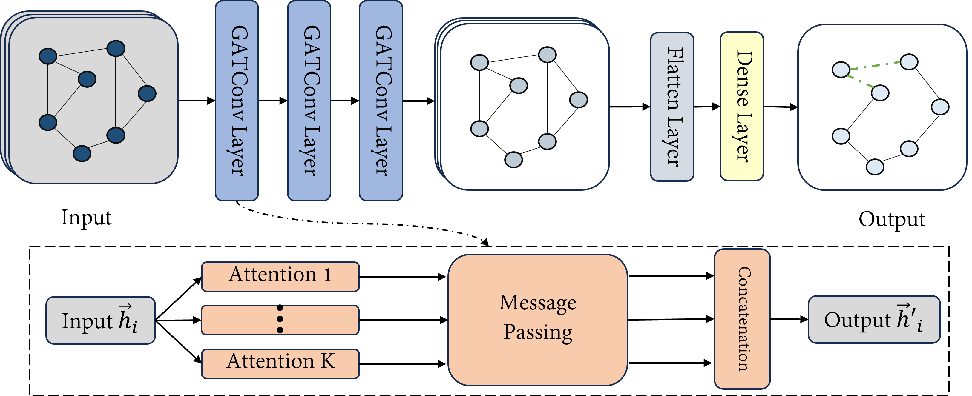
Figure 3: The structure of the GAT-based fault localization algorithm. By using GAT rather than spectral GCN, better performance can be achieved reacting to dynamic changes in the graph structure of the power systems in this study.

It consists of an input layer representing the bus information of the entire power grid, followed by a GAT with $L_{g}$ layers to extract higher-dimensional spatial features of the graph. Subsequently, a flatten layer is employed to collapse the graph structure and convert the output of the GAT into a flat vector. A dense layer then integrates all high-level features to generate a final prediction, and an output layer provides the likelihood that each transmission line in area $H$ is under attack. The architecture of the proposed algorithm is depicted in Fig. 3.

Let $\vec{y}$ denote the output of the dense layer, processed through a sigmoid activation function. After offline training, the output $\vec{y}$ of the GAT-FL algorithm can be used to locate transmission line faults using a threshold. After finishing training, $\vec{y}$ can also be used to construct the parameter vector $\vec{c}$. In the following section, we shall discuss on identification of the actual states of transmission lines within the attacked area given the output of the GAT-FL algorithm.

Remark.

Although Eq. (6) may theoretically admit infinitely many solutions, our hypothesis is that these feasible solutions exhibit a distinctive distribution in a high-dimensional feature space. GAT leverages both graph structure and attention mechanisms to capture the subtle correlations among nodes, effectively modeling the underlying distribution of the ground truth for fault localization. As a result, GAT can robustly locate transmission line faults, even when multiple mathematical solutions to Eq. (6) might exist.

IV-B Line State Identification (LSI) Algorithm

As aforementioned, the islanding caused by physical attacks and the existence of the cycles within the $H$ area may lead to changes in power injection $\vec{p}$ and the presence of multiple solutions for $\vec{x}_{H}$. Meanwhile, failure of the sparsity assumption impairs the LP algorithm (P0) to find the ground truth from these solutions. Using the output $\vec{y}$ from the GAT-FL algorithm, we propose an LSI algorithm to identify the real line state within the $H$ area.

The existence of islanding can be detected by monitoring the bus power injection $\vec{p}_{\bar{H}}$ within the $H$ area under the assumption that the power load on each bus remains unchanged before and after the attack. For instance, if $\vec{p}^{\prime}_{\bar{H}}$ differs from $\vec{p}_{\bar{H}}$ ($\vec{\Delta}_{\bar{H}}\neq\vec{0}$), we conclude that islanding exists within the $H$ area; otherwise, no islanding is present. Such an assessment approach shall allow us to determine the status within the attacked area for both islanding and islanding-free scenarios.

In our case, it is noted that $\vec{\Delta}_{H}$ is unknown when it is not sure if islanding occurs. According to Eq. (6), we give that

$$\vec{\Delta}_{H}=A_{H|G}(\vec{\theta}-\vec{\theta^{\prime}})+D_{H}^{\prime}\vec{x}_{H}.$$ (21)

After a subtle transformation, Eq. (21) can be rewritten in terms of the pair of $(\vec{x}_{H},\vec{\Delta}_{H})$.

$$\left[I-D_{H}^{\prime}\right]\begin{bmatrix}\vec{\Delta}_{H}\\ \vec{x}_{H}\end{bmatrix}=A_{H|G}(\vec{\theta}-\vec{\theta^{\prime}}).$$ (22)

Note that Eq. (22) may not have a unique solution for the pair $(\vec{x}_{H},\vec{\Delta}_{H})$ since the maximum rank of $\left[I-D_{H}^{\prime}\right]$ is $|V_{H}|$ when islanding occurs. For such cases, we cannot directly obtain $\vec{x}_{H}$ by solving Eq. (22).

IV-B1 The recovery of $\vec{\Delta}$

If $\vec{\Delta}_{\bar{H}}=0$, then it follows that $\vec{\Delta}_{H}=0$ as well, indicating no changes in power injections within the $H$ area; otherwise, islanding occurs. In the islanding scenario, it is assumed that the load shedding/generation reduction that resulted from islanding follows the proportional load shedding/generation reduction [32]; such an assumption has been widely adopted in studies on small and medium-scale power systems [33]. Under such an assumption, any pair of buses $\{u,v\}$ within the same island after the attack satisfy:

$${p}^{\prime}_{u}/p_{u}={{p}}^{\prime}_{v}/{p}_{v}.$$ (23)

Based on this assumption, we present the following lemma for recovering the power injection information within the $H$ area.

Lemma 3.

Suppose Assumptions 2 and 3 hold. For all $u\in{\cal V}_{H}$, there exists $v\in{\cal V}_{\bar{H}}$ such that $e=(u,v)\in\cal{E}$. The post-attack power injection $p^{\prime}_{u}$ can be recovered according to Eq. (23).

Proof.

According to Assumption 2, for any bus $u\in{\cal V}_{H}$, there exists an adjacent bus $v\in{\cal V}_{\bar{H}}$ such that $e=(u,v)\in\cal{E}$. Since $v$ is outside the attacked area and its power injection change is known, we can compute the proportion $p^{\prime}_{v}/p_{v}$. Applying Eq. (23), we can then determine the proportional change in power injection at bus $u$. Consequently, $\vec{p}^{\prime}_{H}$ and $\vec{\Delta}^{\prime}_{H}$ can be recovered. ∎

IV-B2 Objective function

Using the information from $\vec{p}^{\prime}_{H}$ and $\vec{\Delta}^{\prime}_{H}$, we can identify the states of transmission lines within the $H$ area. As aforementioned, we aim to incorporate $\vec{c}$ into the objective function of the LP algorithm to prioritize areas with higher risks. By focusing on the most critical components, we can effectively reduce the problem’s practical dimensionality, which helps to improve the solution’s accuracy and enhance computational efficiency. Based on this idea, we denote $\vec{c}=\textbf{1}-\vec{y}$ and present the new problem formulation (P2) as below.

(P2): $$\min_{\vec{x}_{H}}(\textbf{1}-\vec{y})^{T}\vec{x}_{H}$$ (24)

s.t. $$\eqref{eq:assum31},\eqref{eq:assum32},\eqref{eq:assum33},\eqref{eq: 20},$$ (25)

$$0\leq\vec{x}_{H}\leq 1,$$ (26)

where $0\leq\vec{x}_{H}\leq 1$ denotes element-wise inequality and $\vec{y}$ is the output of the GAT-FL algorithm whose elements indicate the probabilities that attacks occur at the corresponding transmission lines. The elements of the parameter vector $\vec{c}=\textbf{1}-\vec{y}$ represent the probabilities that the corresponding transmission lines are free of physical attacks. Therefore, the objective function of (P2) can be interpreted as that physical attacks more likely have happened on those transmission lines with higher $\vec{y}_{i}$ (lower $(1-\vec{y}_{i})$).

We propose the line state identification (LSI) algorithm for identifying the real state within the $H$ area, as shown in Algorithm 1.

Algorithm 1 Line State Identification (LSI) Algorithm.

1: Input: $A$, $D$, $\Gamma$, $\vec{p}$, $\vec{p}^{\prime}_{\bar{H}}$, $\vec{\theta}$, $\vec{\theta}^{\prime}$, $\vec{y}$.

2: Output: Attack vector $\vec{x}_{H}$

3: if $\vec{p}_{\bar{H}}\neq\vec{p}_{\bar{H}}^{\prime}$ then

4:  Recover $\vec{\Delta}_{H}$ using Lemma 3.

5: else

6:  $\vec{\Delta}_{H}\leftarrow\vec{0}$

7: end if

8: Obtain $\vec{x}_{H}$ $\leftarrow$ solving the optimization problem (P2).

9: return  $\vec{x}_{H}$.

V Experimental results

In the numerical simulation, two baseline algorithms are used to conduct the fault localization benchmark test for comparison: failed line detection algorithm (FLD) [23] and GCN [28]. The reason we choose these two algorithms is that FLD and GCN are the state-of-the-art fault localization algorithms for CCPA and short-circuit failures, respectively. We carry out simulations of fault diagnosis scheme on IEEE 30 bus and IEEE 118 bus standard test cases. For the GAT-FL algorithm, we generate a dataset for its training and evaluation.

V-A Data collection

For both IEEE 30/118 bus cases, we connect each bus with a load that is randomly sampled from the load level distribution. The load level distribution is derived from a realistic annual residential load curve, as presented in [34]. To construct PCPA, we randomly partition the entire power grid into $H$ and $\bar{H}$ areas using a degree-based greedy search (DBGS) algorithm for fulfilling Assumptions 1 and 2. Specifically, this algorithm starts from a given seed node and iteratively expands a subgraph by adding one neighbor at a time. At each step, it examines the neighbors of the most recently added node, computes their degrees with respect to nodes outside the current subgraph, and greedily selects the neighbor with the highest external degree to include. Such the algorithm also may generate more possible cycles in the attacked area. In addition, for impedance values of faulty lines, we multiply them by a constant sampled from $(1.5,5)$ and $(100,1000)$ for the admittance-altering and link-cut cases, respectively. The simulations are conducted using MATPOWER [35].

In particular, for each type of attack, we execute the power flow for a sampled load profile to obtain 200 data samples. For an $H$ area with $|{\cal V}_{H}|$ buses and $|{\cal E}_{H}|$ transmission lines, each transmission line has $3$ possible class labels (attack-free, admittance altering, and link cut). To mitigate classification complexity, we simplify the labeling scheme by assigning a label of “$1$” to each attacked line, whether due to admittance altering or disconnection, and a label of “$0$” to all normal operational lines. To be able to locate the attacks effectively, we feed the model with voltage phase angle $\vec{\theta}$ and power injection $\vec{p}$. Furthermore, it is noted that the weighted matrix is designated as $W={\cal A}$, where ${\cal A}$ is the adjacency matrix of graph $\cal G$.

V-B Performance metrics and training platform

To evaluate the performance of our fault localization algorithm, we introduce the accuracy, false alarm rate (FAR), missed detection rate (MDR) and $\text{F}_{1}$ score. Their definition are as follows:

$$\text{Accuracy}=\frac{\text{TP}+\text{TN}}{\text{TP}+\text{FP}+\text{TN}+\text{FN}},$$ (27)

$$\text{FAR}=\frac{\text{FP}}{\text{FP}+\text{TN}},$$ (28)

$$\text{MDR}=\frac{\text{FN}}{\text{TP}+\text{FN}},$$ (29)

$$\text{F}_{1}=\frac{2*\text{TP}}{2\text{TP}+\text{FP}+\text{FN}},$$ (30)

where TP, FP, TN, and FN denote true positives, false positives, true negatives, and false negatives, respectively. To evaluate the performance of the LSI algorithm, we introduce the error term

$$\text{error}=\frac{\|\vec{x}_{\text{ground}}-\vec{x}\|}{\|\vec{x}_{\text{ground}}\|},$$ (31)

where $\vec{x}_{\text{ground}}$ denotes the ground truth of physical attack vector and $\vec{x}$ is the estimation of physical attack vector provided by the LSI algorithm.

All algorithms run on AMD Ryzen Threadripper PRO 3955WX 16-Cores 3.9GHz CPU with $4$ NVIDIA GeForce RTX 3090 GPUs. The implementation of GAT and GCN model is based on PyTorch in Python.

V-C Numerical results

In the following, we illustrate the numerical results obtained by the fault localization algorithm and the LSI algorithm.

V-C1 The performance on the IEEE 30 buses

In this case, we generate a cyclic attacked area $H$ with $|{\cal V}_{H}|=8$ and $|{\cal E}_{H}|=8$ using the DBGS algorithm. The hyperparameters of the GCN model have $3$ graph convolutional layers with $256$ filters for each layer, while the GAT-FL model contains $3$ graph attention layers with $128$ filters for each layer. Both models are followed by dense layers of the same size. The Adam optimizer with an initial learning rate of $0.0001$ is used to train these models 500 times.

Table II shows the performance of the proposed GAT-FL algorithm for fault localization on IEEE 30 bus cases.

TABLE II: Performance Comparison of Fault Localization for Different Methods on IEEE 30 bus case

Method	Metric	Fault Lines
		1	2	3	4	5	6	7
FLD	Accuracy	0.9569	0.8944	0.8375	0.7881	0.7244	0.6644	0.6212
	FAR	0	0	0	0	0	0	0
	MDR	0.3450	0.4225	0.4333	0.4238	0.4410	0.4475	0.4329
	$\text{F}_{1}$	0.7915	0.7322	0.7234	0.7312	0.7171	0.7118	0.7238
GCN	Accuracy	0.8400	0.8050	0.8119	0.7638	0.7556	0.7531	0.7238
	FAR	0.1421	0.1633	0.1630	0.1900	0.2150	0.1800	0.1850
	MDR	0.2850	0.2900	0.2300	0.2825	0.2620	0.2692	0.2893
	$\text{F}_{1}$	0.5277	0.6455	0.7543	0.7523	0.7906	0.8162	0.8183
GAT-FL (Ours)	Accuracy	0.8756	0.8525	0.8494	0.8113	0.8169	0.7856	0.7863
	FAR	0.1057	0.1233	0.1280	0.1562	0.1267	0.1475	0.1200
	MDR	0.2550	0.2200	0.1883	0.2213	0.2170	0.2367	0.2271
	$\text{F}_{1}$	0.5996	0.7256	0.8016	0.8049	0.8424	0.8423	0.8635

For accuracy and $\text{F}_{1}$ score metrics, it is noted that when $|F|=1$, the FLD algorithm outperforms GAT-FL and GCN, especially in the $\text{F}_{1}$ metric. The reason is that the number of fault lines is aligned with the sparsity assumption. When $|F|$ reaches $2$, the performance gap between GAT-FL and FLD is already narrowed to approximately $4\%$ in the accuracy and $1\%$ in the $\text{F}_{1}$ score. As $|F|$ continues to increase, both GAT-FL and GCN show an improved performance, while the performance of FLD drops. For those cases with three or more faulty lines, GAT-FL outperforms FLD by up to $14\%$ and maintains a consistent lead of about $5\%$ over GCN in the $\text{F}_{1}$ score. For false alarm and missed detection metrics, FLD steadily achieves zero false alarms but suffers from the highest missed detection rate. In contrast, GAT-FL maintains both a lowest and stable missed detection rate and a lower false alarm rate compared to GCN, making it more balanced across different fault scenarios. Overall, GAT-FL stands out as the most effective method once $|F|$ exceeds $2$, combining strong detection performance with favorable false alarm and missed detection rates.

The performance of fault diagnosis scheme consisting of GAT-FL algorithm and LSI algorithm has also been examined. The results are shown in Table III.

TABLE III: Mean Estimation Errors of Different Methods on IEEE 30 bus case

Method	Fault Lines
	1	2	3	4	5	6	7
FLD	0.0000	0.0123	0.0487	0.0810	0.1302	0.1323	0.1581
GCN+LSI	0.0111	0.0116	0.0471	0.0763	0.1202	0.1211	0.1498
GAT+LSI (Ours)	0.0111	0.0252	0.0350	0.0715	0.0980	0.1019	0.1344

Given $H$, for different values of $|F|$, we examine these algorithms in $500$ cases with different faulty lines to obtain the mean error. It is noted that the mean estimation error of those three algorithms increases as $|F|$ increases. When $|F|=1$, FLD outperforms GCN+LSI and GAT+LSI while the latter two algorithms have the equivalent performance. GCN+LSI surpasses the other two algorithms at $|F|=2$. However, the proposed GAT+LSI algorithm outperforms the two baselines in the rest of the cases, keeping consistency with the results of fault localization in Table II.

V-C2 The performance on IEEE 118 buses

In this case, we generate an attacked area $H$ with $|{\cal V}_{H}|=12$, $|{\cal E}_{H}|=13$ and $2$ cycles using the DBGS algorithm. The hyperparameters of the GCN model, the proposed GAT-FL model and the following dense layers are set the same as those in the IEEE 30 bus case. The Adam optimizer with an initial learning rate of $0.0001$ is used to train these models 500 times.

TABLE IV: Performance Comparison of Fault Localization for Different Methods on IEEE 118 bus case

Method	Metric	Fault Lines
		1	2	3	4	5	6	7	8	9	10	11	12
FLD	Accuracy	0.9504	0.9269	0.8973	0.8688	0.8419	0.8181	0.7804	0.7546	0.6938	0.6577	0.6215	0.5858
	FAR	0.0312	0.0318	0.0490	0.0439	0.0500	0.0579	0.0567	0.0500	0.0575	0.0550	0.0400	0.0300
	MDR	0.2700	0.3000	0.2817	0.3275	0.3310	0.3267	0.3593	0.3675	0.4167	0.4285	0.4400	0.4462
	$\text{F}_{1}$	0.6936	0.7467	0.7635	0.7594	0.7650	0.7736	0.7586	0.7603	0.7251	0.7198	0.7146	0.7116
GCN	Accuracy	0.8642	0.8662	0.8512	0.8346	0.8273	0.8088	0.8008	0.7850	0.7608	0.7358	0.7250	0.7000
	FAR	0.1304	0.1186	0.1305	0.1417	0.1244	0.1471	0.1317	0.1180	0.1212	0.1500	0.1125	0.1700
	MDR	0.2000	0.2175	0.2100	0.2188	0.2500	0.2425	0.2571	0.2756	0.2917	0.2985	0.3045	0.3108
	$\text{F}_{1}$	0.4755	0.6427	0.7101	0.7440	0.7696	0.7853	0.8006	0.8057	0.8039	0.8033	0.8106	0.8092
GAT-FL (Ours)	Accuracy	0.9562	0.9388	0.9265	0.9231	0.9158	0.9162	0.9046	0.8915	0.8762	0.8565	0.8535	0.8331
	FAR	0.0392	0.0473	0.0640	0.0617	0.0663	0.0693	0.0808	0.0920	0.0887	0.1250	0.0825	0.1000
	MDR	0.1000	0.1375	0.1050	0.1113	0.1130	0.1008	0.1079	0.1187	0.1394	0.1490	0.1582	0.1725
	$\text{F}_{1}$	0.7595	0.8127	0.8490	0.8767	0.8901	0.9082	0.9097	0.9091	0.9058	0.9012	0.9067	0.9015

The performance of the proposed GAT-FL algorithm for fault localization on the IEEE 118 bus case, as shown in Table IV, demonstrates its clear superiority over the FLD and GCN baselines across three key metrics: accuracy, missed detection rate, and $\text{F}_{1}$ score. Notably, the performance gap between GAT-FL and the two baselines becomes more pronounced as the number of faulty lines increases. For example, when $|F|=12$, GAT-FL outperforms GCN by approximately $10\%$ and FLD by around $19\%$ in terms of the $\text{F}_{1}$ score. Furthermore, while FLD achieves the lowest false alarm rate, GAT-FL maintains a competitive false alarm rate, offering a balanced trade-off between minimizing false alarms and excelling in other critical metrics. These results highlight the robustness and effectiveness of GAT-FL in handling complex fault localization scenarios.

TABLE V: Mean Estimation Errors (MSE) of Different Methods on IEEE 118 bus case

Method	Fault Lines
	1	2	3	4	5	6	7	8	9	10	11	12
FLD	0.1961	0.2527	0.2650	0.2901	0.2717	0.2694	0.2684	0.2603	0.2308	0.2134	0.1964	0.1746
GCN+LSI	0.1570	0.1876	0.2188	0.2744	0.2461	0.2638	0.2628	0.2667	0.2359	0.2381	0.2246	0.1985
GAT+LSI (Ours)	0.1476	0.1533	0.1801	0.2100	0.2132	0.2085	0.2234	0.2105	0.1879	0.1985	0.1882	0.1814

For performance comparison of line state identification, the simulation setting is similar to that in IEEE 30 bus case. In Table V, we evaluate the mean estimation errors of the proposed GAT+LSI algorithm and the two baseline methods (FLD and GCN+LSI) for line state identification. The mean estimation errors of all the three methods exhibit an initial increase followed by a subsequent decline. This trend may suggest that, in this attacked area with two cycles, identifying line states in the cases with either very few or many faulty lines is relatively easier compared to that in cases with a moderate number of faulty lines. The proposed GAT+LSI algorithm consistently outperforms FLD when $|F|\leq 9$, maintaining a stable advantage. However, this advantage diminishes as the number of faulty lines increases, with FLD slightly surpassing GAT+LSI at $|F|=12$. Compared to GCN+LSI, the GAT+LSI method consistently achieves lower mean errors, with an improvement range of approximately $0.009$ to $0.065$. This advantage is particularly significant in the interval $4\leq|F|\leq 10$, highlighting the robustness and efficiency of GAT+LSI in handling moderate fault scenarios.

In general, these two sets of numerical simulation results demonstrate the excellent and robust performance of the proposed fault diagnosis scheme, especially in scenarios with complex faults.

VI Conclusion

In this study, we developed a GAT-FL algorithm for fault localization and state estimation for power systems under PCPA. The algorithm is composed of two parts. In the first part, benefiting from the learning ability of GAT to complex pattern on graph data, a GAT-based fault localization algorithm was proposed to assess the likelihood of being faulty for each transmission line within the attacked area. In the second part, a line state identification (LSI) algorithm was designed utilizing LP and the results of the first part. This proposed algorithm can effectively deal with islanding issues and cyclic issues within the attacked area caused by PCPA. Experimental simulations have been conducted on IEEE 30 bus and IEEE 118 bus networks. Simulation results evidently demonstrated the effectiveness of the proposed algorithms.

There are several possible directions for further studies. One is to consider PCPA with more sophisticated, arguably more hostile cyber attacks, e.g., a carefully planned combination of DoS and FDI attacks. Another one, as mentioned earlier, is to design effective algorithms where Assumption 2 does not hold. Yet another development we would like to make is to investigate the effects and develop solutions when there exist strong noises in measurement data.

References

- [1] X. Fang, S. Misra, G. Xue, and D. Yang, “Smart grid—the new and improved power grid: A survey,” IEEE Commun. Surveys Tuts., vol. 14, no. 4, pp. 944–980, 2011.
- [2] A. Abur and A. G. Exposito, Power system state estimation: theory and implementation. CRC press, 2004.
- [3] M. D. Smith and M. E. Paté-Cornell, “Cyber risk analysis for a smart grid: How smart is smart enough? A multiarmed bandit approach to cyber security investment,” IEEE Trans. Eng. Manag., vol. 65, no. 3, pp. 434–447, 2018.
- [4] J. Machowski, Z. Lubosny, J. W. Bialek, and J. R. Bumby, Power system dynamics: stability and control. John Wiley & Sons, 2020.
- [5] A. Hahn and M. Govindarasu, “Cyber attack exposure evaluation framework for the smart grid,” IEEE Trans. Smart Grid, vol. 2, no. 4, pp. 835–843, 2011.
- [6] B. Li, R. Lu, G. Xiao, T. Li, and K.-K. R. Choo, “Detection of false data injection attacks on smart grids: A resilience-enhanced scheme,” IEEE Trans. Power Syst., vol. 37, no. 4, pp. 2679–2692, 2022.
- [7] K. Wang, M. Du, S. Maharjan, and Y. Sun, “Strategic honeypot game model for distributed denial of service attacks in the smart grid,” IEEE Trans. Smart Grid, vol. 8, no. 5, pp. 2474–2482, 2017.
- [8] G. Liang, J. Zhao, F. Luo, S. R. Weller, and Z. Y. Dong, “A review of false data injection attacks against modern power systems,” IEEE Trans. Smart Grid, vol. 8, no. 4, pp. 1630–1638, 2016.
- [9] R. Deng, G. Xiao, and R. Lu, “Defending against false data injection attacks on power system state estimation,” IEEE Trans. Ind. Informat., vol. 13, no. 1, pp. 198–207, 2015.
- [10] Z. Zhang, R. Deng, D. K. Y. Yau, P. Cheng, and J. Chen, “Analysis of moving target defense against false data injection attacks on power grid,” IEEE Trans. Inf. Forensics Security, vol. 15, pp. 2320–2335, 2020.
- [11] W. Xu, I. M. Jaimoukha, and F. Teng, “Robust moving target defence against false data injection attacks in power grids,” IEEE Trans. Inf. Forensics Security, vol. 18, pp. 29–40, 2022.
- [12] Z. Zhang, Y. Tian, R. Deng, and J. Ma, “A double-benefit moving target defense against cyber–physical attacks in smart grid,” IEEE Internet Things J., vol. 9, no. 18, pp. 17 912–17 925, 2022.
- [13] S. Lakshminarayana, E. V. Belmega, and H. V. Poor, “Moving-target defense against cyber-physical attacks in power grids via game theory,” IEEE Trans. Smart Grid, vol. 12, no. 6, pp. 5244–5257, 2021.
- [14] R. M. Lee, “Analysis of the cyber attack on the ukrainian power grid,” 2016, [Online], Available: https://ics.sans.org/media/E-ISAC.
- [15] R. Weinmann, E. Cotilla-Sanchez, and T. K. A. Brekken, “Toward models of impact and recovery of the us western grid from earthquake events,” Energies, vol. 15, no. 24, 2022.
- [16] R. Deng, P. Zhuang, and H. Liang, “CCPA: Coordinated cyber-physical attacks and countermeasures in smart grid,” IEEE Trans. Smart Grid, vol. 8, no. 5, pp. 2420–2430, 2017.
- [17] G. Chen, Z. Y. Dong, D. J. Hill, and Y. S. Xue, “Exploring reliable strategies for defending power systems against targeted attacks,” IEEE Trans. Power Syst., vol. 26, no. 3, pp. 1000–1009, 2010.
- [18] T. Zhou, K. Xiahou, L. Zhang, and Q. Wu, “Real-time detection of cyber-physical false data injection attacks on power systems,” IEEE Trans. Ind. Informat., vol. 17, no. 10, pp. 6810–6819, 2020.
- [19] Y. Chen, S. Lakshminarayana, and F. Teng, “Localization of coordinated cyber-physical attacks in power grids using moving target defense and deep learning,” in IEEE SmartGridComm, 2022, pp. 387–392.
- [20] S. Soltan, M. Yannakakis, and G. Zussman, “Joint cyber and physical attacks on power grids: Graph theoretical approaches for information recovery,” ACM SIGMETRICS Perform. Eval. Rev., vol. 43, no. 1, pp. 361–374, 2015.
- [21] ——, “Power grid state estimation following a joint cyber and physical attack,” IEEE Trans. Control Netw. Syst., vol. 5, no. 1, pp. 499–512, 2018.
- [22] M. J. Hossain and M. Rahnamy-Naeini, “Line failure detection from pmu data after a joint cyber-physical attack,” in IEEE PESGM, 2019, pp. 1–5.
- [23] Y. Huang, T. He, N. R. Chaudhuri, and T. F. La Porta, “Link state estimation under cyber-physical attacks: Theory and algorithms,” IEEE Trans. Smart Grid, vol. 13, no. 5, pp. 3760–3773, 2022.
- [24] C. Zhai, H. Zhang, G. Xiao, and T.-C. Pan, “An optimal control approach to identify the worst-case cascading failures in power systems,” IEEE Trans. Control Netw. Syst., vol. 7, no. 2, pp. 956–966, 2020.
- [25] C. Pei, Y. Xiao, W. Liang, and X. Han, “Pmu placement protection against coordinated false data injection attacks in smart grid,” IEEE Trans. Ind. Appl., vol. 56, no. 4, pp. 4381–4393, 2020.
- [26] O. Boyaci, M. R. Narimani, K. R. Davis, M. Ismail, T. J. Overbye, and E. Serpedin, “Joint detection and localization of stealth false data injection attacks in smart grids using graph neural networks,” IEEE Trans. Smart Grid, vol. 13, no. 1, pp. 807–819, 2022.
- [27] A. Takiddin, R. Atat, M. Ismail, O. Boyaci, K. R. Davis, and E. Serpedin, “Generalized graph neural network-based detection of false data injection attacks in smart grids,” IEEE Trans. Emerg. Topics Comput., 2023.
- [28] K. Chen, J. Hu, Y. Zhang, Z. Yu, and J. He, “Fault location in power distribution systems via deep graph convolutional networks,” IEEE J. Sel. Areas Commun., vol. 38, no. 1, pp. 119–131, 2020.
- [29] P. Veličković, G. Cucurull, A. Casanova, A. Romero, P. Liò, and Y. Bengio, “Graph attention networks,” in ICLR, 2018.
- [30] K. He, D. Yu, D. Wang, M. Chai, S. Lei, and C. Zhou, “Graph attention network-based fault detection for uavs with multivariant time series flight data,” IEEE Transactions on Instrumentation and Measurement, vol. 71, pp. 1–13, 2022.
- [31] Z. Meng, J. Zhu, S. Cao, P. Li, and C. Xu, “Bearing fault diagnosis under multisensor fusion based on modal analysis and graph attention network,” IEEE Transactions on Instrumentation and Measurement, vol. 72, pp. 1–10, 2023.
- [32] P. Kundur, Power System Stability and Control. New York, NY, USA: McGraw-Hill, 1994.
- [33] A. A. Girgis and S. Mathure, “Application of active power sensitivity to frequency and voltage variations on load shedding,” Electric Power Systems Research, vol. 80, no. 3, pp. 306–310, 2010.
- [34] M. Muratori, “Impact of uncoordinated plug-in electric vehicle charging on residential power demand,” Nat. Energy, vol. 3, no. 3, pp. 193–201, 2018.
- [35] R. D. Zimmerman, C. E. Murillo-Sánchez, and R. J. Thomas, “Matpower: Steady-state operations, planning, and analysis tools for power systems research and education,” IEEE Trans. Power Syst., vol. 26, no. 1, pp. 12–19, 2010.
- [36] OpenAI, “ChatGPT: [Large Language Model],” 2023, [Online], Available: https://openai.com/chat.