Ro-To-Go!
Robust Reactive Control with Signal Temporal Logic

Abstract

Signal Temporal Logic (STL) robustness is a common objective for optimal robot control, but its dependence on history limits the robot’s decision-making capabilities when used in Model Predictive Control (MPC) approaches. In this work, we introduce Signal Temporal Logic robustness-to-go (Ro-To-Go), a new quantitative semantics for the logic that isolates the contributions of suffix trajectories. We prove its relationship to formula progression for Metric Temporal Logic, and show that the robustness-to-go depends only on the suffix trajectory and progressed formula. We implement robustness-to-go as the objective in an MPC algorithm and use formula progression to efficiently evaluate it online. We test the algorithm in simulation and compare it to MPC using traditional STL robustness. Our experiments show that using robustness-to-go results in a higher success rate.

I Introduction

Many robotic applications demand complex behaviors that are difficult to specify. Temporal Logics [1] provide a grounded mathematical approach to specify such behaviors. Linear Temporal Logic (LTL) [2] is a popular logic for discrete-time robotic applications. In recent years, there has been a growing interest in logics that describe more complex behaviors than LTL. Metric Temporal Logic (MTL) [3] and Metric Interval Temporal Logic (MITL) [4] extend LTL to reason about continuous time. Signal Temporal Logic (STL) [5] is a subset of MITL defined over real-valued signals, making it particularly useful to robotic applications. In addition to providing a binary answer for whether a signal satisfies a specification, it also admits a quantitative score of how well the signal satisfies it, known as the Robust Satisfaction Value, or simply robustness [6]. This value characterizes how robust a planned trajectory is to unforeseen disturbances.

The state-of-the-art robot control algorithms for STL specifications are based on trajectory optimization techniques, and are split into two distinct approaches. One approach is is to encode the STL specification as mixed integer constraints on an optimization problem. For convex objective functions, this results in a mixed integer convex program (MICP) [7]. Although this approach is complete, the constraints induced by the STL specification introduce new variables for each time step and this scales poorly. This approach also requires both the system dynamics [8] and the logical predicates [9] to be linear. The other approach directly optimizes the STL robustness [10], resulting in a nonlinear programming problem (NLP). This approach allows for nonlinear system dynamics and logical predicates. Although incomplete, this approach scales much better than the MICP approach due to the lack of integer constraints. This makes the NLP approach more practical for most robot control applications, where the robot must react to unforeseen changes in their environment.

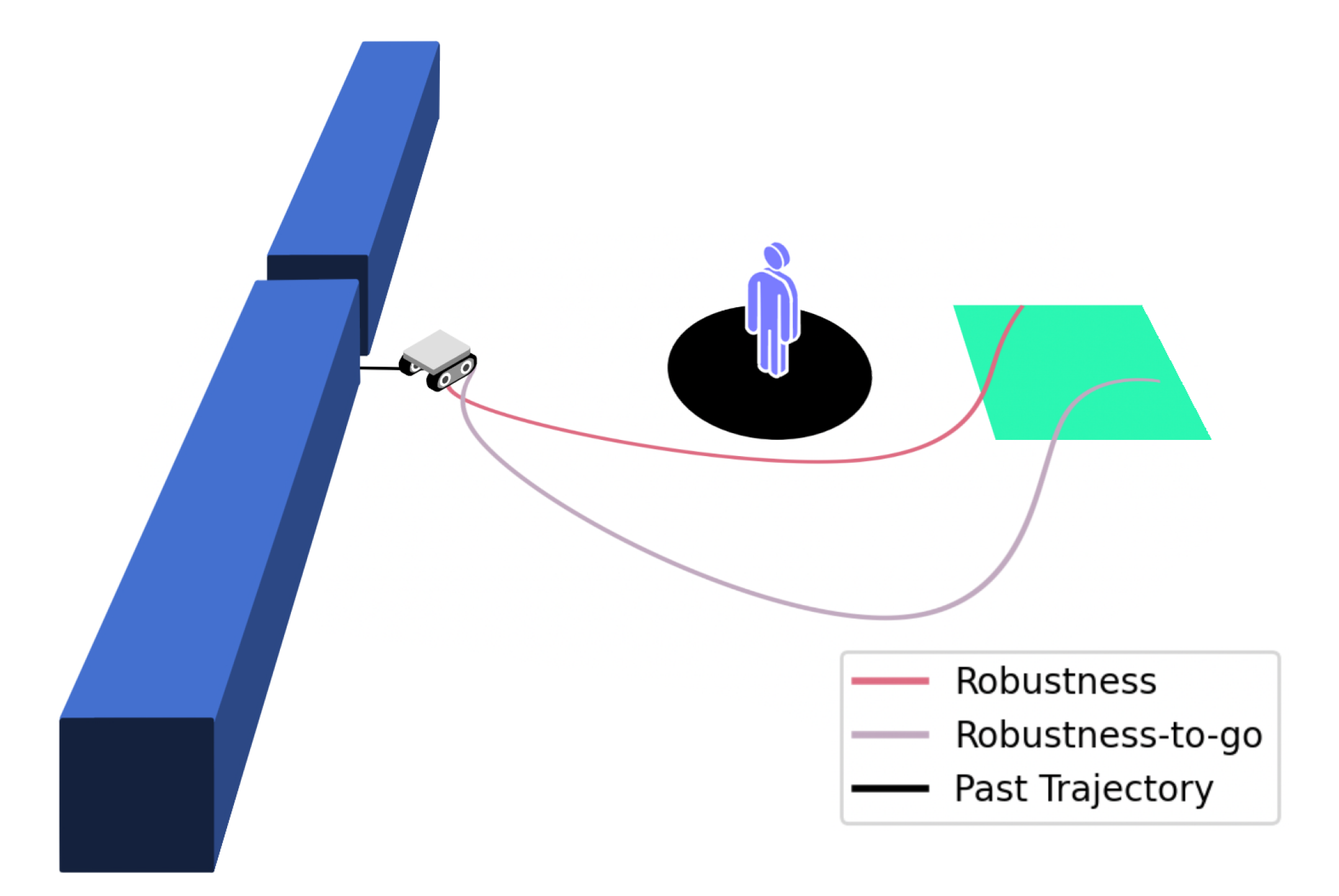
Figure 1: This examples shows a robot planning a path to the goal while avoiding the human. With regular robustness, the proximity to the obstacles at the beginning limits the overall robustness, so there is no value in going further away from the human. With robustness-to-go, the robot has forgotten about its past proximity to the obstacles and can find trajectories that are more robust to human movement.

Consider a practical example, shown in Fig. 1, where a robot must reach a goal within a fixed time limit while avoiding obstacles and humans. For such a mission, the robot might be unaware of how the human will move and must react to the human’s motion.

One approach to achieve such reactive behavior is Model Predictive Control (MPC), which solves the aforementioned optimization problems periodically during mission execution. Given the current state, at each iteration, a new optimal trajectory is computed and executed until the next trajectory is found. This iterative replanning gives MPC approaches some level of resilience to dynamic environments.

While the STL robustness is a sound objective function for open-loop control synthesis, it has shortcomings in the context of feedback control through MPC. This is because the robustness is a function of the entire trajectory, and so the history of the robot’s motion is considered in the objective function. If the robot comes close to violating the specification, then all of its plans from that point onward are limited in how robust they can be. The robot cannot distinguish between good and bad trajectories because the robustness does not provide any incentive for the robot to move further away from future possible violations. Fig. 1 captures this phenomenon. Both trajectories have the same robustness due to their proximity to obstacles at the beginning, even though the blue trajectory steers further from the human.

In this paper, we introduce robustness-to-go, a new robustness measure designed to reason about the suffix of trajectories, the portion beyond a given time. This measure scores the trajectory from the given time onwards, instead of scoring the past trajectory of the robot. At each MPC planning step, we use robustness-to-go (Ro-To-Go) as our objective function, enabling the robot to remain robust to future disturbances, regardless of its past. We prove that Ro-To-Go can be efficiently calculated by using MITL Formula Progression [11], a technique that rewrites formulas iteratively after each observation.

The contributions of this paper are (i) introduction of robustness-to-go, a new STL robustness measure that focuses on reasoning about suffix trajectories, (ii) a technique to efficiently calculate the robustness-to-go using formula progression (iii) proofs of the soundness of the measure and its relationship to formula progression, and (iv) a series of case studies investigating the incorporation of this measure in a feedback control algorithm, and its impact on robot behavior.

II Related Work

Control synthesis for STL specifications was first investigated in [7], where they extend an MICP-approach to synthesis for LTL specifications from [12] to handle STL specifications. This approach automatically generates a set of mixed integer linear constraints for an optimal control problem. If the system is linear and the objective function is convex, then the optimal solution can be found using a MICP [9].

These encodings only apply to STL formulas over linear predicates. Furthermore, nonlinear systems turn the optimization problem into a mixed-integer non-convex program, which is intractable. Therefore, instead of encoding the STL specification as mixed integer constraints, an alternate approach formulates an optimization problem where the specification is instead considered in the objective function, via the robustness measure. This approach still results in a nonconvex optimization problem, but finding local optima is faster because of the lack of integer constraints. The notion of optimizing temporal logic robustness was first introduced in [13], in the context of minimizing MTL robustness for verification purposes. Robustness is a highly discontinuous function, and so the authors in [10] propose a smooth approximation of MTL robustness, and use gradient ascent tools to maximize it for control synthesis purposes. The works [14], [15], [16] extend this approach to optimize smooth approximations of STL robustness.

Robustness as an objective function, however, has its shortcomings. Called locality in [17], traditional robustness characterizes trajectories by their most critical point, that is, the point that is the requires the smallest alteration to change the satisfaction result. In the context of open-loop control synthesis, this is a reasonable objective to optimize for: Making the most critical point more robust to disturbances makes the entire trajectory more robust to disturbances. In feedback control, however, the most critical point could be a point in the past, that has already happened. The result of this is that all plans will be limited by this point, and the robot has trouble distinguishing trajectories that are better ”from here on out” from others. Works [8] and [18] attempt to better characterize the entire trajectory by defining new ”average” STL robustness measures to optimize for. Recently, the authors in [17] generalize these robustness measures, among others, by introducing Generalized Mean Robustness. These measures are not subject to the locality effect, meaning that the robot can distinguish between two trajectories whose most critical points are the same. In contrast, our approach aims to disregard this most critical point entirely if it is in the past. We propose robustness-to-go, a measure that is defined on the suffix of trajectories. While still local, the most critical point for a formula’s robustness-to-go is within the planning horizon of the robot. Robustness-to-go is an orthogonal concept to the works of [8], [18], and [17], and can be combined with them to form average-robustness-to-go measures.

III Preliminaries

Let $x\in X\subseteq\mathbb{R}^{n}$ be a state, and time domain $\mathcal{T}$ be a set of time instants such that $\mathcal{T}\subseteq\mathbb{R}_{\geq 0}$. Then, a signal $s$ is a mapping from $\mathcal{T}$ to $X$, and sample from the signal is $(t,s(t))$.

A signal predicate $\mu$ is a formula of the form $f(x)>0$, where $f:X\rightarrow\mathbb{R}$. We express properties of signals with respect to signal predicates using signal temporal logic (STL) [5].

Definition 1 (STL Syntax). The STL Syntax is recursively defined by:

$$\varphi:=\top\ |\ \mu\ |\ \lnot\phi\ |\ \phi\land\phi\ |\ \phi U_{I}\psi$$ (1)

where $\phi$ and $\psi$ are STL formulas,$I=\langle a,b\rangle$ is a time interval with $\langle\in\{(,[\},\rangle\in\{),]\}$, and $0\leq a<b\leq\infty$. Notation $\top$, $\lnot$, and $\land$ are Boolean ”true”, ”negation” and ”conjunction,” respectively, and U denotes the temporal ”until” operator.

Logical disjunction can be expressed as $\phi\lor\psi=\lnot(\lnot\phi\land\lnot\psi)$, logical implication as $\phi\rightarrow\psi=(\lnot\phi)\lor\psi$, and ”false” as $\bot=\lnot\top$. The temporal operator eventually ($\Diamond_{I}\phi$) can be expressed as $\top U_{I}\phi$ and the temporal operator globally ($\square_{I}\phi$) can be expressed as $\lnot\Diamond_{I}\lnot\phi$. The interval $I+c=\langle a+c,b+c\rangle$.

Definition 2 (STL Semantics). The semantics of STL is defined over a signal s at time t as:

$$(s,t)\vDash\top \iff\top$$

$$(s,t)\vDash f(x)>0 \iff f(s(t))>0$$

$$(s,t)\vDash\lnot\phi \iff(s,t)\nvDash\phi$$

$$(s,t)\vDash\phi\land\psi \iff(s,t)\vDash\phi\land(s,t)\vDash\psi$$

$$(s,t)\vDash\phi U_{I}\psi \iff\exists t^{\prime}\in I+t\ s.t.(s,t^{\prime})\vDash\psi$$

$$\quad\quad\ \ \land\forall t^{\prime\prime}\in[t,t^{\prime}),(s,t^{\prime\prime})\vDash\phi$$

where $\vDash$ denotes satisfaction. A signal s satisfies an STL formula $\varphi$ if $(s,0)\vDash\varphi$

In this work, we consider the set $\mathcal{T}$ to be finite and strictly increasing, and employ discrete-time, or pointwise, semantics. Refer to [19] and [20] for a discussion on the differences between continuous and pointwise semantics.

The authors in [11] show that, under pointwise semantics, we can incrementally track the satisfaction of MTL formulas using formula progression. We adapt it here for STL.

Definition 3 (STL Formula Progression). Given an STL formula $\varphi$, a time step $\Delta$, and an observation of a state $x$, the progressed formula is given by $\varphi^{+}=P(\varphi,\Delta,x)$:

$$P(\top,\Delta,x) =\top$$

$$P(\bot,\Delta,x) =\bot$$

$$P(f(x)>0,\Delta,x) =\begin{cases}\top\text{ if }f(x)>0\\ \bot\text{ otherwise }\end{cases}$$

$$P(\lnot\phi,\Delta,x) =\lnot P(\phi,\Delta,x)$$

$$P(\phi\land\psi,\Delta,x) =P(\phi,\Delta,x)\land P(\psi,\Delta,x)$$

$$P(\phi U_{I}\psi,\Delta,x) =\begin{cases}P(\phi,\Delta,x)\land\phi U_{I^{\leftarrow}_{\Delta}}\psi&\text{if }0<I\\ P(\psi,\Delta,x)\lor&\\ \ \ (P(\phi,\Delta,x)\land\phi U_{I^{\leftarrow}_{\Delta}}\psi)&\text{if }0\in I,\end{cases}$$

where $I^{\leftarrow}_{\Delta}=(I-\Delta)\cap\mathbb{R}_{\geq 0}$ and $\phi U_{\emptyset}\psi=\bot$.

Note that we have added a truncation operation to the definition from [11] because STL intervals must have positive endpoints. Here, $I^{\leftarrow}$ is the subset of $I-\Delta$ that is greater than or equal to zero. When the interval $I$ in $\phi U_{I}\psi$ is the empty set $\emptyset$, the temporal operator resolves to false. This is also why, unlike [11], we have no case for the until operator where $0>I$. The truncation operation prevents such cases from happening.

In addition to qualitative semantics, STL also admits quantitative semantics, known as the robust satisfaction value, or simply robustness.

Definition 4 (STL Robust Satisfaction Value). The quantitative semantics of STL is defined over a signal s at time t as:

$$\rho(s,t,\top) =\infty$$

$$\rho(s,t,f(x)>0) =f(s(t))$$

$$\rho(s,t,\lnot\phi) =-\rho(s,t,\phi)$$

$$\rho(s,t,\phi\land\psi) =\min\{\rho(s,t,\phi),\rho(s,t,\psi)\}$$

$$\rho(s,t,\phi U_{I}\psi) =\sup_{t^{\prime}\in I+t}\min\begin{pmatrix}\rho(s,t^{\prime},\psi),\\ \inf\limits_{t^{\prime\prime}\in[t,t^{\prime})}{\rho(s,t^{\prime\prime},\phi)}\\ \end{pmatrix}$$

A signal s satisfies an STL formula $\varphi$ if $\rho(s,0,\varphi)>0$.

Definition 5 (STL Time Horizon). The Time Horizon of an STL formula $[\varphi]^{\uparrow}$ is the horizon which a signal can impact the satisfaction of $\varphi$:

$$[\varphi]^{\uparrow} =\begin{cases}0&\text{ if }\varphi\in\{\top,\mu\}\\ [\phi]^{\uparrow}&\text{ if }\varphi=\lnot\phi\\ \max\{[\phi]^{\uparrow},[\psi]^{\uparrow}\}&\text{ if }\varphi=\phi\land\psi\\ b+\max\{[\phi]^{\uparrow},[\psi]^{\uparrow}\}&\text{ if }\varphi=\phi U_{\langle a,b\rangle}\psi\\ \end{cases}$$

A formula is bounded if $[\varphi]^{\uparrow}<\infty$, or unbounded otherwise.

IV Problem Formulation

Consider a discrete time robotic system of the form

$$x^{r}_{t+\Delta}=\tilde{f}(x^{r}_{t},u_{t})$$ (2)

where $x^{r}\in X^{r}\subset\mathbb{R}^{n_{r}}$ is the state of the robot and $u\in U\subset\mathbb{R}^{m}$ is the control input. The environment’s dynamics are captured similarly in discrete time by

$$x^{e}_{t+\Delta}=x^{e}_{t}+w,$$ (3)

where $x^{e}\in X^{e}\subset\mathbb{R}^{n_{e}}$ is the state of the environment and $w\in W\subset\mathbb{R}^{n_{e}}$ captures an unknown disturbance in environment’s dynamics. The environment can capture dynamic yet not controllable aspects of the world that are relevant to the task. This can include not only a dynamic physical environment, but also other robots and even humans acting in the same space as the robot.

We wish to specify tasks as bounded STL formula over the composed robot-environment system. For a specification $\varphi$, we consider time domain $\mathcal{T}=\{0,\Delta,2\Delta,...,[\varphi]^{\uparrow}\}$. Our signal is a mapping $s:\mathcal{T}\rightarrow X^{r}\times X^{e}\times U\times W$. We denote the components of $s$ using subscripts, i.e., the robot state component of signal $s$ at time $t$ is $s_{x^{r}}(t)$. A signal $s$ is valid if the robot and environment components follow from the input and disturbance components according to equations 2 and 3, i.e., $s_{x^{r}}(t+\Delta)=\tilde{f}(s_{x^{r}}(t),s_{u}(t))$ and $s_{x^{e}}(t+\Delta)=s_{x^{e}}(t)+s_{w}(t)$, for all $t\in[0,[\varphi]^{\uparrow}-\Delta]$.

We first present the motion planning problem. Given that the robot finds motion plans iteratively for closed-loop feedback control, it will find motions during execution. Because STL satisfaction depends on the robot’s future and past, the robot must consider its history. Let $s^{t}$ be a signal defined over $[0,t]$ such that $t<\infty$. $s^{t}$ is a prefix of s if, for all $t^{\prime}\leq t,s(t^{\prime})=s^{t}(t^{\prime})$.

Problem 1 Given system (2), environment (3), bounded STL task $\varphi$, and signal prefix $s^{t}$, find $s$ such that (i) $s\vDash\varphi$, (ii) $s^{t}$ is a prefix of $s$, (iii) $s_{w}(t^{\prime})=s_{w}(t)\ \forall t^{\prime}\ \in[t,[\varphi]^{\uparrow}]$, and (iv) $s$ is valid.

Note the constraint on $s_{w}(t^{\prime})$. Because the environment disturbances $w$ are unknown a-priori, Problem IV assumes a static environment. Due to this, there are no guarantees on the safety of the closed-loop controller. However, by integrating solutions to Problem IV in an MPC loop, subsequent solutions plan for the updated environment state, allowing the robot to react to the unknown environment disturbances.

V Ro-To-Go!

Solutions to Problem IV include both the NLP and MICP approaches discussed in section I. The MICP approach introduces extra constraints to ensure $s\vDash\varphi$, and optimize for some other convex objective function [7]. The NLP approach involves optimizing the robustness, or some other robustness measure [17]. They find $\max_{S}\rho(s,0,\varphi)$, and $s\vDash\varphi$ if the optimization converges on a local optima such that $\rho(s,0,\varphi)>0$.

We are interested in the NLP solution to Problem IV in the context of MPC. The robustness depends on the entire trajectory, meaning that the robot must consider the past as a prefix $s^{t}$, and the robot only plans for the suffix. As the MPC algorithm iterates and the robot executes the mission, the portion of the trajectory that the robot can control shrinks. In many instances, the portion of the trajectory in the past, outside of the robot’s control, dominates the robustness. The impact of this is that the portion of the trajectory that the robot can control does not have a big impact on the robustness, and the robot cannot easily distinguish between different behaviors.

Ideally, the robot should focus on what it can control, and find the most robust behaviors within that window. To this end, we propose robustness-to-go (Ro-To-Go).

Definition 6 (STL Robustness-To-Go). The robustness-to-go from time $\hat{t}$ of STL formula $\varphi$ is defined over a signal s at time t as:

$$\rho^{\looparrowright}(s,t,\hat{t},\top) =\infty$$

$$\rho^{\looparrowright}(s,t,\hat{t},f(x)>0) =\begin{cases}f(s(t))&\text{ if }t>\hat{t}\\ \infty\cdot\text{sign}(f(s(t)))&\text{ otherwise}\\ \end{cases}$$

$$\rho^{\looparrowright}(s,t,\hat{t},\lnot\phi) =-\rho^{\looparrowright}(s,t,\hat{t},\phi)$$

$$\rho^{\looparrowright}(s,t,\hat{t},\phi\land\psi) =\min\{\rho^{\looparrowright}(s,t,\hat{t},\phi),\rho^{\looparrowright}(s,t,\hat{t},\psi)\}$$

$$\rho^{\looparrowright}(s,t,\hat{t},\phi U_{I}\psi) =\sup_{t^{\prime}\in I+t}\min\begin{pmatrix}\rho^{\looparrowright}(s,t^{\prime},\hat{t},\psi),\\ \inf\limits_{t^{\prime\prime}\in[t,t^{\prime})}{\rho^{\looparrowright}(s,t^{\prime\prime},\hat{t},\phi)}\\ \end{pmatrix}$$

Ro-To-Go differs from traditional robustness in how it treats predicates. When the predicate robustness is evaluated after some user-specified $\hat{t}$, it is evaluated exactly like traditional robustness. If, however, the predicate robustness is evaluated before $\hat{t}$, the robustness is instead $\infty$ or $-\infty$, depending on if the predicate is satisfied or not.

We propose solving Problem IV by optimizing for the Ro-To-Go from the planning time onwards. This approach is sound because Ro-To-Go itself is a sound robustness measure.

Theorem 1 (Soundness). A signal s satisfies an STL formula if and only if it has a positive robustness-to-go, i.e. $(s,t)\vDash\varphi\iff\rho^{\looparrowright}(s,t,\hat{t},\varphi)>0$. This holds regardless of $\hat{t}$

Proof:

Proof by induction on the structure of STL. The full proof is in Appendix A.

Example 1 (Robustness-to-go.) Consider the formula $\varphi_{avoid}=\square_{[0,20]}(\lnot(\text{human}\lor\text{obs}_{1}\lor\text{obs}_{2}))\land\Diamond_{[0,20]}\text{goal}$, which specifies that the robot must avoid the human and obstacles for twenty seconds, and reach the goal within twenty seconds. Here, human, goal, obs₁ and obs₂ are defined as

$$\text{human}= (x-x_{e})^{2}+(y-y_{e})^{2}<0.25$$

$$\text{obs}_{1}= (x>0.5\land x<1\land y>0\land y<2.4)$$

$$\text{obs}_{2}= (x>0.5\land x<1\land y>2.6\land y<5)$$

$$\text{goal}= (x>4\land y>2\land y<3).$$

Fig. 1 shows the robot planning for these specifications, during the mission. The robot has already executed a prefix trajectory, and began close to $\text{obs}_{1}$ and $\text{obs}_{2}$, at $(0.5,2.5)$. Because of this, all trajectories beginning from this initial state will have a robustness of at most 0.1. Indeed, the red line in Fig. 1 shows the robot coming within 0.13 meters of the human. This is because, when using robustness, the robot could not distinguish between this trajectory and one that goes further from the human. In contrast, the Ro-To-Go from the planning point onwards does not consider the contribution of the initial point, but only the contribution from the points within the plan under consideration. As such, it can better distinguish between good and bad motion plans, finding a plan that only comes within 0.79 meters of the human. The plan found using Ro-To-Go is safer with respect to unforeseen human motion.

VI Formula Progression for STL Ro-To-Go

Ro-To-Go is a function of the entire trajectory signal. As such, when planning trajectories during mission execution, the history of the robot’s motion must be considered. During planning, these iterative Ro-To-Go evaluations must consider the same past. Because the robot cannot change the past, processing this data is redundant. In this section, we show how to use formula progression from Definition III to avoid these redundant operations. Informally, we show that the Ro-To-Go from time $\hat{t}$ is the same as the robustness of the progressed formula at time $\hat{t}$.

Theorem 2 Let $\phi_{0}$ be an STL formula, $s$ be a signal, and consider sample $(t_{i},s(t_{i}))$. Let $\Phi=\{\phi_{0},\phi,...,\phi_{i+1}\}$ be a set of STL formulas such that $\phi_{k}=P(\phi_{k-1},t_{k}-t_{k-1},s(t_{k-1}))$ for each $0<k\leq n$. Then,

$$t_{i}\geq t_{0}\rightarrow\rho(s,t_{i+1},\phi_{i+1})=\rho^{\looparrowright}(s,t_{0},t_{i},\phi_{0})$$

Proof Sketch. This proof involves proving the following through induction on the structure of STL:

$$\rho^{\looparrowright}(s,t_{k},\hat{t},\varphi)$$ (4)

$$=\begin{cases}\rho(s,t_{k},\varphi)&\text{ if }\hat{t}<t_{k}\\ \rho(s,t_{k+1},P(\varphi,t_{k+1}-t_{k},s(t_{k})))&\text{ if }\hat{t}=t_{k}\\ \rho^{\looparrowright}(s,t_{k+1},\hat{t},P(\varphi,t_{k+1}-t_{k},s(t_{k})))&\text{ if }\hat{t}>t_{k}\\ \end{cases}.$$

Then, we prove Theorem VI by induction through time from Equation 4. The full proof is in Appendix A. $\hfill\blacksquare$

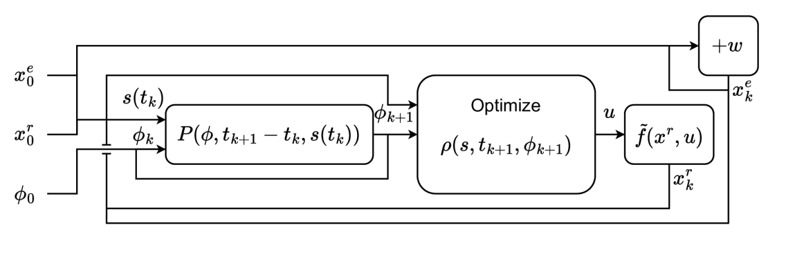
Figure 2: Control Block Diagram for Ro-To-Go MPC with Formula Progression

Fig. 2 shows how to incorporate formula progression for MPC with Ro-To-Go. The approach begins by using the initial robot state, environment state, and STL formula $\phi_{0}$ to find the progressed formula $\phi_{k+1}$. In the NLP optimization problem, we optimize the robustness of trajectories with respect to $\phi_{k+1}$, beginning from the next time step $t_{k+1}$. According to Theorem VI, the optimization objective $\rho(s,t_{k+1},\phi_{k+1})$ is the Ro-To-Go of the original formula from the initial point onwards $\rho^{\looparrowright}(s,t_{0},t_{0},\phi_{0})$. Note that, even though the first point evaluated is $t_{k+1}$, the state at $t_{k}$ must still be considered to ensure that trajectories are valid. Once the optimal solution is found, the robot applies control input $u$, and the environment evolves according to its unknown motion. The next iteration begins, with the progressed formula $\phi_{k+1}$ becoming $\phi_{,}$, and the new robot and environment states become $s(t_{k})$. For a given planning iteration at time $t_{i}$, the robot is optimizing the Ro-To-Go of the original formula from the current time onwards $\rho^{\looparrowright}(s,t_{0},t_{i},\phi_{0})$.

Using formula progression to find the Ro-To-Go has two major benefits. The first is that it avoids reprocessing of past observations. This is because the robustness of the progressed formula depends only on points within the robot’s planning horizon. The second benefit is that, by reducing the problem of calculating Ro-To-Go to the problem of calculating robustness, we can exploit readily available tools for calculating robustness such as Breach [22] or STLRom [25]. Similarly, using formula progression paves the road for combining Ro-To-Go with other robustness measures, such as those discussed in [17].

VII Experiments

We have implemented Ro-To-Go for use in solving Problem IV using VP-STO [23], a state-of-the-art motion planning and MPC algorithm which uses CMA-ES [24] as the black box optimization technique. CMA-ES is gradient-free and thus can handle discontinuous objective functions, making it a good fit for STL robustness. To calculate the STL robustness while planning, we use STLRom [25].

We consider a system with double-integrator dynamics, i.e., $\dot{x}=v_{x},\dot{y}=v_{y},\dot{v_{x}}=a_{x},\dot{v_{y}}=a_{y},$ where $a_{x}$ and $a_{y}$ are the control inputs. The environment state is $[x_{e},y_{e}]^{T}$, and receives a random perturbation $w=[w_{1},w_{2}]^{T}$, where $w_{1},w_{2}\sim\mathcal{N}(0,4)$, every 0.02 seconds.

For our experiments, we examine the task described by $\varphi_{avoid}$ from example V and

$$\varphi_{stayIn} =\square_{[0,20]}\text{region, where}$$

region $$=(x(t)-x_{e}(t))^{2}+(y(t)-y_{e}(t))^{2}<2,$$

which specifies that the robot must remain within some region for twenty seconds. Fig. 3 show the environments for $\varphi_{avoid}$ and $\varphi_{stayIn}$.

To evaluate the impact of using Ro-To-Go as an objective function in an MPC algorithm, we benchmark its performance and compare it against the performance when using traditional robustness as an objective function. For our two formulas, we run both algorithms 100 times and report the average performance.

To evaluate our approach against real-time requirements, we have implemented the algorithm in a simulated environment in the Robot Operating System (ROS) [26]. The planning time is not fixed, and runs concurrently to the application of control. During execution, the robot will follow the most recent motion plan. The hyperparameters for the experiments are given in Appendix LABEL:sec:_params.

VII-A Results

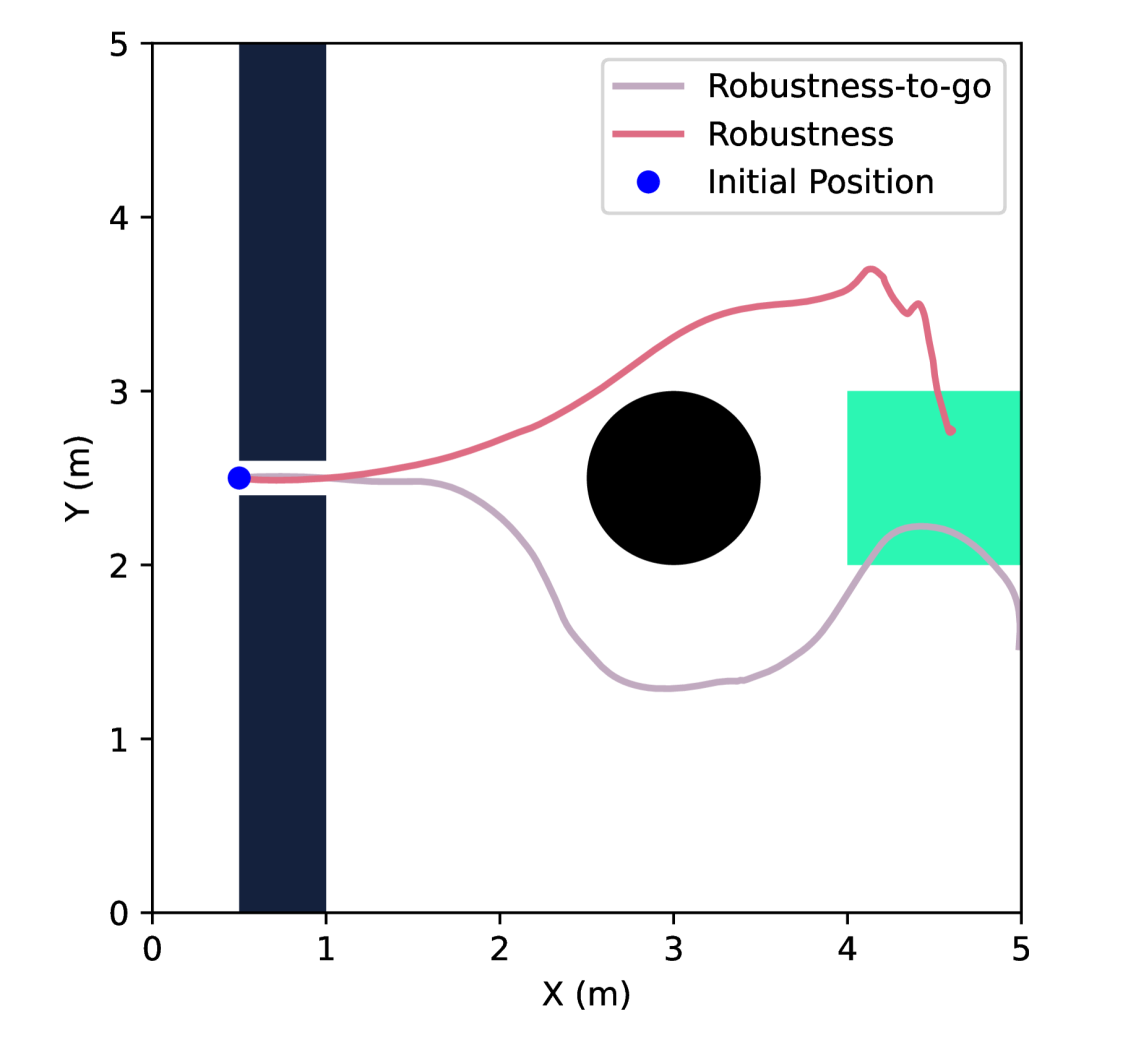
(a) $\varphi_{avoid}$

(b) $\varphi_{stayIn}$

Figure 3: Sample trajectories for both formulas, simulated with a static environment

Problem	Robustness	Min Distance	Success Rate
$\varphi_{avoid}$, Robustness	-0.421	0.172	0.63
$\varphi_{avoid}$, Ro-To-Go	-0.079	0.312	0.91
$\varphi_{stayIn}$, Robustness	0.341	-1.278	0.76
$\varphi_{stayIn}$, Ro-To-Go	0.601	-1.379	0.99

TABLE I: Statistics of 100 runs of each approach against two STL specifications

Figs. 3(a) and 3(b) show two closed-loop trajectories from both algorithms, when simulated in a static environment. Fig. 3(a) shows that the robot better avoids the human when using Ro-To-Go as an objective function, when compared to traditional robustness. This is because the proximity to the obstacles at the beginning of the mission is not considered when evaluating the Ro-To-Go, but is when using robustness. Similarly, Fig. 3(b) shows that the robot stays near the middle of the region when using Ro-To-Go, but wanders when using robustness. Again, this is because the initial proximity to the edge of the region is ”forgotten” once the robot begins executing the mission.

Note the end of the simulated trajectory when using Ro-To-Go in Fig. 3(a): It does not go deeper into the goal and instead leaves it. Indeed, once the robot has entered the goal region, that aspect of the mission is completely satisfied and is not considered in the Ro-To-Go afterwards. One interpretation of this behavior is that the robot displays more robust behavior under ”globally” ($\square$) type formulas, and less robust behavior under ”eventually” ($\Diamond$) type formulas. In the context of MPC, however, there is a more practical interpretation. STL robustness represents a trajectory’s robustness to change. Because the past cannot change, satisfying points in the past are in some sense infinitely robust. There is no disturbance that would cause this past satisfaction to become a violation, and so planning to satisfy it more robustly can be wasteful.

Table I shows the benchmarking results, now simulated with a dynamic environment. For $\varphi_{avoid}$, we see that the average robustness value is higher when using Ro-To-Go. It is, however, still negative. This is due to the proximity to the obstacles at the beginning of the simulation - the maximum achievable robustness for both is 0.1, and so failures have a big impact on the average. It is more informative, instead, to examine the average minimum distance from the region. The robot stays much further from the region when using Ro-To-Go, consistent with the behavior from Fig. 3(a).

For $\varphi_{stayIn}$, we also see higher average robustness when using Ro-To-Go. Here, the minimum distance to the goal is negative because the robot wants to stay inside of the region. The lower value when using Ro-To-Go means that the robot reached closer to the center of the region.

For both formulas, we see a higher success rate when using Ro-To-Go, reflecting its safety benefits.

VIII Conclusion and Future Work

The main contribution of this paper is STL robustness-to-go (Ro-To-Go), a new quantitative semantics for the logic, along with proofs of its relationship to MTL formula progression. This robustness measure addresses some shortcomings of traditional STL robustness in the context of feedback control for robotic systems. We implement both robustness and robustness-to-go as the objective in an MPC algorithm, and find that robustness-to-go outperforms traditional robustness.

For future work, we will investigate the relationship between robustness-to-go, which focuses on the contribution of suffix trajectories, to the Robust Satisfaction Interval (RoSI) [27], which focuses on the contribution of prefix trajectories.

Appendix A Proofs

A-A Proof of Theorem V

A signal s satisfies an STL formula if and only if it has a positive robustness to go, i.e.

$$(s,t)\vDash\varphi\iff\rho^{\looparrowright}(s,t,\hat{t},\varphi)>0$$

References

- [1] N. Rescher and A. Urquhart, Temporal logic. Springer Science & Business Media, 2012, vol. 3.
- [2] A. Pnueli, “The temporal logic of programs,” in 18th annual symposium on foundations of computer science (sfcs 1977). ieee, 1977, pp. 46–57.
- [3] R. Koymans, “Specifying real-time properties with metric temporal logic,” Real-time systems, vol. 2, no. 4, pp. 255–299, 1990.
- [4] R. Alur, T. Feder, and T. A. Henzinger, “The benefits of relaxing punctuality,” Journal of the ACM (JACM), vol. 43, no. 1, pp. 116–146, 1996.
- [5] O. Maler and D. Nickovic, “Monitoring temporal properties of continuous signals,” in International symposium on formal techniques in real-time and fault-tolerant systems. Springer, 2004, pp. 152–166.
- [6] A. Donzé and O. Maler, “Robust satisfaction of temporal logic over real-valued signals,” in International Conference on Formal Modeling and Analysis of Timed Systems. Springer, 2010, pp. 92–106.
- [7] V. Raman, A. Donzé, M. Maasoumy, R. M. Murray, A. Sangiovanni-Vincentelli, and S. A. Seshia, “Model predictive control with signal temporal logic specifications,” in 53rd IEEE Conference on Decision and Control, 2014, pp. 81–87.
- [8] N. Mehdipour, C.-I. Vasile, and C. Belta, “Arithmetic-geometric mean robustness for control from signal temporal logic specifications,” in 2019 American Control Conference (ACC). IEEE, 2019, pp. 1690–1695.
- [9] C. Belta and S. Sadraddini, “Formal methods for control synthesis: An optimization perspective,” Annual Review of Control, Robotics, and Autonomous Systems, vol. 2, no. 1, pp. 115–140, 2019.
- [10] Y. V. Pant, H. Abbas, and R. Mangharam, “Smooth operator: Control using the smooth robustness of temporal logic,” in 2017 IEEE Conference on Control Technology and Applications (CCTA). IEEE, 2017, pp. 1235–1240.
- [11] F. Bacchus and F. Kabanza, “Planning for temporally extended goals,” Annals of Mathematics and Artificial Intelligence, vol. 22, pp. 5–27, 1998.
- [12] E. M. Wolff, U. Topcu, and R. M. Murray, “Optimization-based trajectory generation with linear temporal logic specifications,” in 2014 IEEE International Conference on Robotics and Automation (ICRA). IEEE, 2014, pp. 5319–5325.
- [13] H. Abbas and G. Fainekos, “Computing descent direction of mtl robustness for non-linear systems,” in 2013 American Control Conference. IEEE, 2013, pp. 4405–4410.
- [14] Y. V. Pant, H. Abbas, R. A. Quaye, and R. Mangharam, “Fly-by-logic: Control of multi-drone fleets with temporal logic objectives,” in 2018 ACM/IEEE 9th International Conference on Cyber-Physical Systems (ICCPS). IEEE, 2018, pp. 186–197.
- [15] Y. Gilpin, V. Kurtz, and H. Lin, “A smooth robustness measure of signal temporal logic for symbolic control,” IEEE Control Systems Letters, vol. 5, no. 1, pp. 241–246, 2020.
- [16] R. Takano, H. Oyama, and M. Yamakita, “Continuous optimization-based task and motion planning with signal temporal logic specifications for sequential manipulation,” in 2021 IEEE international conference on robotics and automation (ICRA). IEEE, 2021, pp. 8409–8415.
- [17] N. Mehdipour, C.-I. Vasile, and C. Belta, “Generalized mean robustness for signal temporal logic,” IEEE Transactions on Automatic Control, 2024.
- [18] L. Lindemann and D. V. Dimarogonas, “Robust control for signal temporal logic specifications using discrete average space robustness,” Automatica, vol. 101, pp. 377–387, 2019.
- [19] P. Bouyer, U. Fahrenberg, K. G. Larsen, N. Markey, J. Ouaknine, and J. Worrell, “Model checking real-time systems,” Handbook of model checking, pp. 1001–1046, 2018.
- [20] H. Abbas, Y. V. Pant, and R. Mangharam, “Temporal logic robustness for general signal classes,” in Proceedings of the 22nd ACM International Conference on Hybrid Systems: Computation and Control, 2019, pp. 45–56.
- [21] Ilyes, R. et al., “Ro-to-go! robust reactive control with signal temporal logic,” arXiv preprint, 2025.
- [22] A. Donzé, “Breach, a toolbox for verification and parameter synthesis of hybrid systems,” in Computer Aided Verification, T. Touili, B. Cook, and P. Jackson, Eds. Berlin, Heidelberg: Springer Berlin Heidelberg, 2010, pp. 167–170.
- [23] J. Jankowski, L. Brudermüller, N. Hawes, and S. Calinon, “Vp-sto: Via-point-based stochastic trajectory optimization for reactive robot behavior,” in 2023 IEEE International Conference on Robotics and Automation (ICRA). IEEE, 2023, pp. 10 125–10 131.
- [24] N. Hansen, “The cma evolution strategy: A tutorial.”
- [25] A. Donzé, Decyphir et. al. Stlrom. [Online]. Available: https://github.com/decyphir/STLRom
- [26] Stanford Artificial Intelligence Laboratory et al. Robotic operating system. [Online]. Available: https://www.ros.org
- [27] J. V. Deshmukh, A. Donzé, S. Ghosh, X. Jin, G. Juniwal, and S. A. Seshia, “Robust online monitoring of signal temporal logic,” Formal Methods in System Design, vol. 51, pp. 5–30, 2017.