Preparing Tetra-Digit Long-Range Entangled States via Unified Sequential Quantum Circuit

Abstract

The quest to systematically prepare long-range entangled phases has gained momentum with advances in quantum circuit design, particularly through sequential quantum circuits (SQCs) that constrain entanglement growth via locality and depth constraints. This work introduces a unified SQC framework to prepare ground states of Tetra-Digit (TD) quantum spin models—a class of long-range entangled stabilizer codes labeled by a four-digit index $[d_{n},d_{s},d_{l},D]$—which encompass Toric Codes across dimensions and the X-cube fracton phase as special cases. Featuring a hierarchical structure of entanglement renormalization group, TD models host spatially extended excitations (e.g., loops, membranes, and exotic non-manifold objects) with constrained mobility and deformability, and exhibit system-size-dependent ground state degeneracies that scale exponentially with a polynomial in linear sizes. We demonstrate the unified SQC through low-dimension examples first, graphically and algebraically, and then extend to general cases, with a detailed proof for the effectiveness of general SQC given in the appendix. With experimental feasibility via synthetic dimensions in quantum simulators, this framework bridges a great variety of gapped long-range entangled states cross dimensions through quantum circuits and shows plentiful mathematical and physical structures in TD models. Through unifying previously disparate preparation strategies, it offers a pathway toward engineered topological phases and fault-tolerant technologies.

I Introduction

Searches for topologically ordered phases [1, 2] in condensed matter materials remain vital for advancing our understanding of exotic quantum phases of matter beyond the Landau-Ginzburg-Wilson paradigm. However, driven by synergies between quantum many-body theory and quantum information science—as well as rapid progress in quantum technologies—researchers have increasingly turned to preparing these exotic states in qubit-based systems. Such engineered quantum states not only enable controlled manipulation and measurement but also bridge theoretical insights into topological order with practical advancements in quantum simulation technologies [3].

Along this line, local quantum circuits (QCs) have been applied to prepare interesting quantum states, which are also systematically categorized by their computational complexity—closely aligned with the classification of quantum phases in condensed matter physics. For gapped states (including topologically ordered phases and product states), two states connected by a finite-depth local unitary (LU) circuit belong to the same phase (when symmetry is not considered) [4], while connecting topologically distinct gapped phases requires at least a linear-depth LU circuit (depth proportional to system’s linear size). Practically, QCs for preparing quantum states initialize from product states of disentangled qubits on lattices. To prepare topologically ordered states that support at most area-law entanglement entropy, linear-depth QCs must be properly designed to constrain entanglement growth—a constraint satisfied by sequential quantum circuits (SQCs) [5, 6, 7, 8, 9, 10, 11, 12].

To realize QCs between two topologically distinct gapped states, Ref. [12] formalized SQCs as local unitary circuits where each qubit is acted upon finitely. To the best of our knowledge, recent advances further leverage SQCs to: (i) construct non-invertible symmetries [13, 14, 15], (ii) engineer Cheshire strings for 3+1D charge condensation [16], (iii) represent gauging procedures [17], (iv) implement non-Abelian anyon ribbon operators [18]. While there has been tremendous progress in SQC proposals, it is increasingly important to find a more unified SQC algorithm that can dismantle barriers between spatial dimensions, liquid states and non-liquid states [19] (e.g., fracton topological phases), and phases from distinct schemes of entanglement renormalization group (ERG) [20, 21, 22].

In this paper, we propose a unified SQC to prepare a large class of topologically ordered states called Tetra-Digit (TD) states, which are ground states of TD models [23]. It is worth noting that Toric Codes across all dimensions, as well as X-cube stabilizer codes, are naturally included as special cases of TD states. Leaving technical details to the main text, we briefly introduce below (i) what TD models (and their associated TD states) are and (ii) why they are of interest.

TD models were first proposed in Ref. [23] and further studied in Refs. [24, 22]. These quantum spin-$1/2$ models are uniquely labeled by a four-digit index $[d_{n},d_{s},d_{l},D]$. Since this class of models was not assigned an official name in Refs. [23, 24, 22], we simply adopt the term “Tetra-Digit (TD) models” in this work. The digit $D$ denotes the spatial dimension of the hypercubic lattice hosting the model. The remaining digits—$d_{n}$, $d_{s}$, and $d_{l}$—characterize microscopic details such as spin (qubit) placements, which will be reviewed technically in Sec. II. Notably, the $[0,1,2,2]$ model corresponds to the 2-dimensional Toric Code; the $[0,1,2,3]$ model describes the 3-dimensional X-cube fracton phase (see, e.g., Refs. [25, 26, 27, 21, 28, 29, 30, 31, 32, 33, 34, 35, 23, 24, 22, 36, 37, 38, 39, 40]); the $[1,2,3,3]$ model represents the 3-dimensional Toric Code. To ensure exact solvability and stabilizer-code ground states, the digits must satisfy specific algebraic constraints.

The original motivation for constructing TD models in Ref. [23] was to extend fracton physics—traditionally focused on point-like topological excitations (e.g., fractons, lineons, planons)—to scenarios involving spatially extended excitations such as loops and membranes. Before the age of fracton physics, such excitations with nonlocal geometry have widely appeared in higher-dimensional topological phases of matter where exotic braiding statistics [41, 42, 43, 44, 45, 46, 47, 48, 49, 50, 51, 52, 53, 54, 55, 56, 57, 58, 59, 60, 61, 62, 63, 64, 65], topological response [66, 67, 68, 69, 70, 71, 72], and symmetry fractionalization [73, 74, 75] go beyond two-dimensional systems. In conventional fracton systems like the X-cube model, fractons are point-like and immobile. Introducing spatially extended objects necessitates considering not only mobility but also deformability, significantly broadening the scope of fracton topological order. Such extended topological excitations are commonly found as excited states in three- and higher-dimensional topologically ordered phases where anyonic particles are absent. Furthermore, in the TD model series, complex excitations with non-manifold-like shapes—neither loops nor membranes—are discovered, exhibiting extreme diversity in both quantum many-body physics and quantum entanglement.

Notably, fracton physics has expanded to encompass many-body systems with Hamiltonians conserving higher moments, such as dipoles (i.e., center-of-mass) [76, 77, 78, 79, 80, 81, 82, 83, 84, 85, 86, 87, 88, 89, 90, 91, 92, 93, 94, 95, 96, 97, 98, 99, 100, 101, 102, 103, 104, 105, 106, 107, 108, 109, 110, 111, 112, 113, 114, 115, 116, 117, 118, 119, 120, 121, 122, 123, 124, 125, 126, 127, 128, 129, 130, 131, 132]. These conserved quantities restrict the kinematics of constituent particles, leading to novel quantum phenomena in equilibrium and non-equilibrium settings. Consequently, the mobility and deformability constraints on spatially extended objects are anticipated to exhibit even more exotic behavior—a problem that remains unresolved.

Following the proposal of TD models, Ref. [24] revealed that their ground state degeneracy (GSD) formulas—expressed as $\text{log}_{2}\text{GSD}$—exhibit diverse polynomial dependencies on system size. This enriches the linear dependence seen in the X-cube model and expands the counting of logical qubits. While a proof is demanded, the polynomial coefficients are conjectured to encode topological and geometric properties of both the quantum codes and the underlying lattice, as demonstrated for the X-cube model in Ref. [21]. In Ref. [22], the origin of the polynomial dependence is connected to a substantially generalized entanglement renormalization group (ERG) program, expanding the definitions of equivalence relations between gapped phases.

While Toric Codes and X-cube states, as special examples of TD states, lack finite-temperature transitions, a subset of TD states ($[1,2,3,D]$ with $D\geq 4$) can host finite-temperature phase transitions [133]. These exotic features and potential applications motivate methods to experimentally prepare TD states. In principle, any 4-dimensional TD model can be realized by synthetically engineering the extra dimension [134, 135, 136]—a strategy extendable to higher-dimensional stabilizer code TD models.

In this paper, we provide an explicit and unified SQC framework for preparing TD states. Concretely, we demonstrate the SQC step by step, explicitly creating the equal weight superposition of configurations (EWSCs) on a particular set of $D$-cubes. Then, we find a set of stabilizer redundancies, by using which we show the EWSCs on all $D$-cubes exist in the final state, explicitly or implicitly. While the primary focus is on SQCs for periodic boundary conditions (PBC), we demonstrate that truncating these circuits (discussed in Sec. III.5) yields SQCs for open boundary conditions (OBC) and hybrid half-PBC-half-OBC configurations—crucial for experimental implementations in finite-size quantum simulators. In the formula of SQC’s total depth (i.e. Eq. (106)), the so called long range entanglement (LRE) level [22] naturally emerges. By explicitly constructing SQCs for key examples such as the $[1,2,3,4]$ and $[2,3,4,4]$ models, we illustrate the framework’s adaptability to higher-dimensional systems. Ultimately, our framework advances the systematic preparation of exotic topological orders across dimensions, bridging theoretical insights with experimental quantum circuit design and opening avenues for exploring unresolved questions in fracton physics and quantum memory applications.

This paper is organized as follows: In Sec. II, we first introduce TD models, refining their definition beyond Ref. [23], and subsequently review their key properties. We then briefly discuss non-stabilizer code TD models, highlighting their distinctions from stabilizer-based cases. In Sec. III, we develop SQC incrementally—starting with the 2-dimensional Toric Code, i.e., the ground state of $[0,1,2,2]$ model, advancing to the ground states of X-cube model (i.e., $[0,1,2,3]$ model), $[0,1,2,4]$ model and 3-dimensional Toric Code model (i.e., $[1,2,3,3]$ model), and finally culminating in a unified SQC framework applicable to generic TD models. To illustrate this framework, we exhibit SQCs for two representative models in detail: $[1,2,3,4]$ and $[2,3,4,4]$, elucidating their implementation within the unified formalism. Finally, Sec. IV concludes the paper and outlines future directions. Some technical details are given in appendices.

II TD models and TD states

II.1 Notations

The TD models constitute a family of spin lattice models defined on $D$-dimensional (hyper)cubic lattices [23]. As their construction inherently involves higher-dimensional geometric constructs (e.g., membranes, volumes), we first establish dimension-agnostic notations. Building on the foundational framework of Refs. [23, 24, 22], we refine the model definitions using terminology from algebraic topology and foliation theory. These additions not only streamline the characterization of spin placements and interactions but also generalize the lattice-dependent structure—enabling future extensions to non-cubic lattices. Crucially, this reformulation preserves the models’ definition while clarifying their geometric-topological underpinnings.

We first review the geometric framework of TD models, following the notation and terminology established in Refs. [23, 24, 22]. Consider a $D$-dimensional (hyper)cubic lattice $\mathbb{Z}_{L_{1}}\times\mathbb{Z}_{L_{2}}\times\cdots\times\mathbb{Z}_{L_{D}}$ with lattice constant 1, subject to open (OBC), periodic (PBC), or half-OBC-half-PBC. The lattice spans $D$ orthogonal directions $\hat{x}_{1},\hat{x}_{2},\ldots,\hat{x}_{D}$. An $n$-cube $\gamma_{n}$ denotes the $n$-dimensional analog of a cube: (i) $0$-cube = vertex, (ii) $1$-cube = edge, (iii) $2$-cube = plaquette, (iv) $3$-cube = 3-dimensional cube, and (v) $4$-cube = 4-dimensional hypercube, and so forth. Each $n$-cube represents a unit cell of the lattice. By fixing the origin at $(0,0,\ldots,0)$ in Cartesian coordinates, the geometric center of every $n$-cube $\gamma_{n}$ has coordinates where exactly $D-n$ components are integers and $n$ components are half-integers. This unique coordinate mapping provides a one-to-one identification of $n$-cubes. A leaf (or leaf space) $l=\langle\hat{x}_{i_{1}},\hat{x}_{i_{2}},\cdots,\hat{x}_{i_{d_{l}}}\rangle$ is defined as a subspace extending along $d_{l}$ orthogonal directions [23]. Leaves partition the lattice into lower-dimensional substructures critical for defining TD models.

The language introduced in the last paragraph is natural for discussing TD models. However, some descriptions could be more precise. In the following several paragraphs, we aim to enhance precision by utilizing terminologies from algebraic topology and foliation theory of manifolds. Readers not interested in these details may skip them.

We begin with a smooth $D$-dimensional manifold with corners $(X,\mathcal{A})$, where the topological manifold $X=T^{m}\times B^{D-m}$ has a cubical cellular decomposition $\mathcal{E}$, with $n$-cells being $n$-cubes, and $\mathcal{A}$ is the atlas. As defined in [137], a manifold with boundary is a special case of a manifold with corners, while a manifold without boundary is a special case of a manifold with boundary. Unless specified otherwise, “manifold” hereafter refers to a manifold with corners. The cubical cellular decomposition $\mathcal{E}$ is the set of all (open) $n$-cubes for all $0\leq n\leq D$. The pair $(X,\mathcal{E})$ is called a cell complex and, since all cells are $n$-cubes, it is also referred to as a cubical complex. For simplicity, we sometimes say $X$ is a cell or cubical complex. Note that, in general, a cell complex $X$ need not be a manifold; it is sufficient for it to be a topological space. Physicists may intuitively consider the $D$-dimensional lattice as the set of all vertices $X^{0}$, or the union of all vertices and edges $X^{1}$. These two sets are known as the 0-skeleton $X^{0}$ and 1-skeleton $X^{1}$ of the cell or cubical complex $X$, respectively. For any $n$, the $n$-skeleton of $X$ is a subcomplex of $X$. A subcomplex of a cell complex $X$ is a closed subspace $A\subset X$ that is a union of cells of $X$.

Now, we turn to leaves. As a smooth manifold (possibly with corners), we can define smooth foliations on $(X,\mathcal{A})$ [138]. A $d_{l}$-dimensional smooth foliation on $(X,\mathcal{A})$ is an equivalence relation on $(X,\mathcal{A})$, with the equivalence classes being connected, disjoint $d_{l}$-dimensional smooth submanifolds called (smooth) leaves. Since we have defined manifolds to refer to manifolds with corners in general, it is worth emphasizing that leaves can only have boundary and corners at the boundary/corners of the original manifold $X$: cutting a complete leaf into two pieces with additional boundary/corners is forbidden. With this restriction, one can freely define different foliations to obtain different leaves. The leaves of interest in this paper are those $d_{l}$-dimensional (smooth) leaves that are simultaneously subcomplexes of $X$, which we call subcomplex leaves hereafter. Subcomplex leaves are exactly those leaves defined in Ref. [23], here with a more rigorous and mathematical definition.

II.2 Hamiltonian

Next, we review the definition of TD models. TD models (and their associated TD states) are labeled by four non-negative integers $[d_{n},d_{s},d_{l},D]$, where $d_{n}\leq d_{s}\leq d_{l}\leq D$. The most distinguishing feature of this model family is that they host fracton orders in arbitrary spatial dimensions greater than two. Such high-dimensional fracton orders possess intriguing properties, such as spatially extended excitations with restricted mobility and deformability, and complex excitations with non-manifold-like shapes [23].

The Hamiltonian of a TD model contains two kinds of stabilizer terms, called $A$ terms and $B$ terms. By our convention, an $A$ term is the product of Pauli $X$ operators, and a $B$ term is the product of Pauli $Z$ operators. In the label $[d_{n},d_{s},d_{l},D]$, $d_{n}$ is the dimension of the cube/cell where we define a $B$ term (“n” stands for “node”), $d_{s}$ is the dimension of the cube/cell where we place a spin (“s” stands for “spin”), $d_{l}$ is the dimension of the leaf where a $B$ term is fully embedded (“l” stands for “leaf”), and $D$ simultaneously stands for the spatial dimension and the dimension of the cube/cell where we define an $A$ term. The Hamiltonian is:

$$H_{[d_{n},d_{s},d_{l},D]}=-\sum_{\gamma_{D}}A_{\gamma_{D}}-\sum_{\gamma_{d_{n}}}\sum_{l\mathchoice{\rotatebox[origin={c}]{180.0}{{\hbox{\subset}}}}{\rotatebox[origin={c}]{180.0}{{\hbox{\subset}}}}{\rotatebox[origin={c}]{180.0}{{\hbox{\scriptstyle\subset}}}}{\rotatebox[origin={c}]{180.0}{{\hbox{\scriptscriptstyle\subset}}}}\gamma_{d_{n}}}B_{\gamma_{d_{n}},l},$$ (1)

where

$$A_{\gamma_{D}}:=\prod_{\gamma_{d_{s}}\subset\gamma_{D}}X_{\gamma_{d_{s}}}$$ (2)

is the product of Pauli $X$ operators of all spins inside the (closed) $D$-cube $\gamma_{D}$, and

$$B_{\gamma_{d_{n}},l}:=\prod_{\begin{subarray}{c}\gamma_{d_{s}}\\ \gamma_{d_{n}}\subset\gamma_{d_{s}}\subset l\end{subarray}}Z_{\gamma_{d_{s}}}$$ (3)

is the product of Pauli $Z$ operators of all spins on the (closed) $d_{s}$-cube $\gamma_{d_{s}}$ that simultaneously contains the node $\gamma_{d_{n}}$ and is inside the leaf $l$. The leaves $l$ in the summation take all possible leaves of the form $\langle\hat{x}_{i_{1}},\hat{x}_{i_{2}},\dots,\hat{x}_{i_{d_{l}}}\rangle$ that simultaneously contain a straightforward $d_{l}$-dimensional sublattice and $\gamma_{d_{n}}$, assuming the $D$-dimensional hypercubic lattice is a direct discretization of Euclidean space. For example, consider the $[0,1,2,3]$ model under OBC, where the 3-dimensional cubic lattice is taken to be a regular lattice in Euclidean space. A leaf can be regarded as a truncated vector/Euclidean space, and in the Hamiltonian, $l$ takes through $\langle\hat{x}_{1},\hat{x}_{2}\rangle$, $\langle\hat{x}_{1},\hat{x}_{3}\rangle$, and $\langle\hat{x}_{2},\hat{x}_{3}\rangle$, each containing $\gamma_{0}$ in the summation $\sum_{l\mathchoice{\rotatebox[origin={c}]{180.0}{$\subset$}}{\rotatebox[origin={c}]{180.0}{$\subset$}}{\rotatebox[origin={c}]{180.0}{$\scriptstyle\subset$}}{\rotatebox[origin={c}]{180.0}{$\scriptscriptstyle\subset$}}\gamma_{0}}$. An illustration of this example is shown in Fig. 1.

Figure 1: Leaves in the $[0,1,2,3]$ TD model (3-dimensional X-cube fracton phase) under open boundary conditions. The black dot denotes a $0$-dimensional node $\gamma_{0}$ at $(1,2,1)$. Three orthogonal leaves (2-dimensional planes) containing $\gamma_{0}$ are highlighted: $\langle\hat{x}_{1},\hat{x}_{2}\rangle$ (red, $x_{3}=1$ plane), $\langle\hat{x}_{1},\hat{x}_{3}\rangle$ (green, $x_{2}=2$ plane), and $\langle\hat{x}_{2},\hat{x}_{3}\rangle$ (blue, $x_{1}=1$ plane). Each leaf hosts $B$ terms formed by products of Pauli $Z$ operators on spins (qubits) within the respective plane. The axes $\hat{x}_{1}$, $\hat{x}_{2}$, $\hat{x}_{3}$ are marked in blue.

In Ref. [23], it has been proven that when the labels satisfy

$$C_{d_{l}-d_{n}}^{d_{s}-d_{n}}\mod 2=0,$$ (4)

$[A_{\gamma_{D}},B_{\gamma_{d_{n}},l}]=0$, the $[d_{n},d_{s},d_{l},D]$ model is a stabilizer code model. In this paper, we primarily focus on the models where Eq. (4) is satisfied. In Sec. II.5, we provide a brief discussion of TD models that are not stabilizer codes, which have been less studied previously.

II.3 Examples

II.3.1 2-dimensional Toric Code as $[0,1,2,2]$ model

The 2-dimensional Toric Code is a prototypical model of pure topological order. The 2-dimensional Toric Code on a square lattice is the $[0,1,2,2]$ model in the TD model family; we show this equivalence now. Consider the 2-dimensional Toric Code on a square lattice, where each edge is assigned a qubit. The Hamiltonian is

$$H=-\sum_{p}A_{p}-\sum_{v}B_{v}=-\sum_{p}\prod_{e\subset p}X_{e}-\sum_{v}\prod_{e\mathchoice{\rotatebox[origin={c}]{180.0}{{\hbox{\subset}}}}{\rotatebox[origin={c}]{180.0}{{\hbox{\subset}}}}{\rotatebox[origin={c}]{180.0}{{\hbox{\scriptstyle\subset}}}}{\rotatebox[origin={c}]{180.0}{{\hbox{\scriptscriptstyle\subset}}}}v}Z_{e},$$ (5)

where $v$, $e$, and $p$ stand for vertex, edge, and plaquette, respectively. An illustration of the $A$ term and $B$ term is shown in Fig. 2. By definition, $v$, $e$, and $p$ correspond to $\gamma_{0}$, $\gamma_{1}$, and $\gamma_{2}$, respectively. Thus, $A_{p}$ can be written as $A_{\gamma_{2}}$, and $B_{v}$ can be written as $B_{\gamma_{0},l}$, where $l$ has only one possible choice (since $d_{l}=2$), i.e., $l$ spans the entire 2-dimensional cubical complex, so the index $l$ can be omitted.

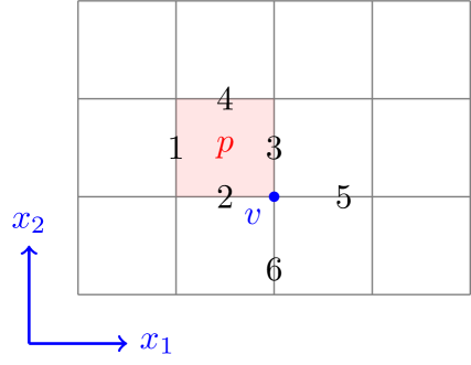
Figure 2: Illustration of $A$ terms and $B$ terms in the 2-dimensional Toric Code. The $A$ term associated with plaquette $p$ is $A_{p}=\prod_{e\subset p}X_{e}=X_{1}X_{2}X_{3}X_{4}$. The $B$ term associated with vertex $v$ is $B_{v}=\prod_{e\mathchoice{\rotatebox[origin={c}]{180.0}{$\subset$}}{\rotatebox[origin={c}]{180.0}{$\subset$}}{\rotatebox[origin={c}]{180.0}{$\scriptstyle\subset$}}{\rotatebox[origin={c}]{180.0}{$\scriptscriptstyle\subset$}}v}Z_{e}=Z_{2}Z_{3}Z_{5}Z_{6}$.

The dimension of $v$ (to which $B$ terms attach) is $0$, so $d_{n}=0$. The dimension of $e$ (where qubits reside) is $1$, so $d_{s}=1$. The leaf dimension $d_{l}=2$. The dimension of $p$ (where $A$ terms reside) is 2, same to the lattice dimension, so $D=2$. Therefore, the 2-dimensional Toric Code on a square lattice is indeed the $[0,1,2,2]$ model.

II.3.2 X-cube as $[0,1,2,3]$ model

The X-cube model is a prototypical example of type-I fracton order [139]. The X-cube model on a cubic lattice is the $[0,1,2,3]$ model in the TD model family; we demonstrate this equivalence now. Consider the X-cube model on a cubic lattice where each edge hosts a qubit. The Hamiltonian is:

$$H=-\sum_{c}A_{c}-\sum_{v}\left(B_{v,xy}+B_{v,xz}+B_{v,yz}\right),$$ (6)

where $A_{c}=\prod_{e\subset c}X_{e}$ is the product of Pauli $X$ operators on all edges of cube $c$, and $B_{v,xy}$ denotes the product of four Pauli $Z$ operators forming an “X” configuration in the $xy$-plane (similarly for $B_{v,xz}$ and $B_{v,yz}$). Fig. 3 illustrates these operators.

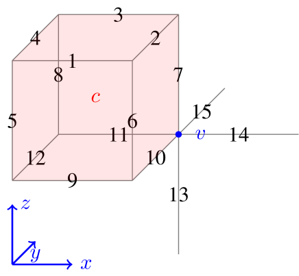
Figure 3: Illustration of $A$ terms and $B$ terms in the X-cube model. The $A$ term associated with cube $c$ is $A_{c}=X_{1}X_{2}\cdots X_{12}$. The three different $B$ terms attached to vertex $v$ are $B_{v,xy}=Z_{10}Z_{11}Z_{15}Z_{14}$, $B_{v,xz}=Z_{7}Z_{11}Z_{13}Z_{14}$, and $B_{v,yz}=Z_{7}Z_{10}Z_{13}Z_{15}$.

The vertex dimension $d_{n}=0$ (to which $B$ terms attach), edge dimension $d_{s}=1$ (where qubits reside), leaf dimension $d_{l}=2$, and lattice dimension $D=3$ (also the dimension of cubes where $A$ terms reside). Thus, the X-cube model corresponds to $[0,1,2,3]$, with Hamiltonian:

$$H =-\sum_{c}A_{c}-\sum_{v}\sum_{l\mathchoice{\rotatebox[origin={c}]{180.0}{$\subset$}}{\rotatebox[origin={c}]{180.0}{$\subset$}}{\rotatebox[origin={c}]{180.0}{$\scriptstyle\subset$}}{\rotatebox[origin={c}]{180.0}{$\scriptscriptstyle\subset$}}v}B_{v,l}.$$ (7)

The X-cube model exhibits a ground state degeneracy (GSD) of $2^{2L_{x}+2L_{y}+2L_{z}-3}$ under PBC, encoding $2L_{x}+2L_{y}+2L_{z}-3$ logical qubits. This extensive degeneracy significantly exceeds that of three-dimensional pure topological orders.

The X-cube model hosts two fundamental excitations:

• Fractons: Created by Pauli $Z$ operators on dual lattice planes, appearing as immobile quadrupoles at cube corners signaled by $A_{c}=-1$. Pairs form mobile planons confined to planes.

• Lineons: Created by Pauli $X$ operators along lines, with three types:

  • $l_{x}$ ($B_{v,xy}=B_{v,xz}=-1$): Moves along $x$-axis

  • $l_{y}$ ($B_{v,xy}=B_{v,yz}=-1$): Moves along $y$-axis

  • $l_{z}$ ($B_{v,xz}=B_{v,yz}=-1$): Moves along $z$-axis

Lineons obey fusion rules $l_{x}\times l_{y}=l_{z}$ [139, 23, 140], demonstrating nontrivial interplay between fracton fusion and mobility.

II.3.3 $[0,1,2,4]$ model

The $[0,1,2,4]$ model is defined on a 4-dimensional hypercubic lattice where each edge hosts a qubit. The Hamiltonian is:

$$H=-\sum_{\gamma_{4}}A_{\gamma_{4}}-\sum_{\gamma_{0}}\sum_{l\mathchoice{\rotatebox[origin={c}]{180.0}{{\hbox{\subset}}}}{\rotatebox[origin={c}]{180.0}{{\hbox{\subset}}}}{\rotatebox[origin={c}]{180.0}{{\hbox{\scriptstyle\subset}}}}{\rotatebox[origin={c}]{180.0}{{\hbox{\scriptscriptstyle\subset}}}}\gamma_{0}}B_{\gamma_{0},l},$$ (8)

where $A_{\gamma_{4}}=\prod_{e\subset\gamma_{4}}X_{e}$ is the product of Pauli $X$ operators on all edges in the 4-cube $\gamma_{4}$, and $B_{\gamma_{0},l}=\prod_{\gamma_{1}\mathchoice{\rotatebox[origin={c}]{180.0}{$\subset$}}{\rotatebox[origin={c}]{180.0}{$\subset$}}{\rotatebox[origin={c}]{180.0}{$\scriptstyle\subset$}}{\rotatebox[origin={c}]{180.0}{$\scriptscriptstyle\subset$}}\gamma_{0},\gamma_{1}\subset l}Z_{e}$ acts on four edges containing vertex $\gamma_{0}$ within a 2-dimensional leaf $l$. Each vertex $\gamma_{0}$ has $C_{4}^{2}=6$ distinct leaves ($d_{l}=2$) in the $D=4$ lattice: $x_{1}x_{2}$, $x_{1}x_{3}$, $x_{1}x_{4}$, $x_{2}x_{3}$, $x_{2}x_{4}$, and $x_{3}x_{4}$ planes. Fig. 4 illustrates these operators.

(a)

(b)

Figure 4: Illustration of $A$ term and $B$ term in the $[0,1,2,4]$ model. The spins are on edges, and the numbers in this figure are placed at the center of each edge, representing the spin on it. (a) The $A$ term associated with 4-cube $\gamma_{4}$ is $A_{\gamma_{4}}=X_{1}X_{2}\cdots X_{32}$, supported by all the edges of $\gamma_{4}$. The dashed cube aids visualizing $x_{4}$-direction edges: the centers of edges spanning in $x_{4}$-direction coincide with the centers of vertices of the dashed cube. (b) Each $B$ term attached to vertex $v$ is supported by 4 edges on a cross containing $v$, e.g. $B_{\gamma_{0},x_{2}x_{3}}=Z_{1}Z_{2}Z_{3}Z_{4}$, $B_{\gamma_{0},x_{3}x_{4}}=Z_{1}Z_{2}Z_{7}Z_{8}$. There are 6 distinct $B$ terms attached to the vertex $v$ due to the combinatorial factor $C_{D-d_{n}}^{d_{l}-d_{n}}=C_{4-0}^{2-0}=6$, which are $B_{\gamma_{0},x_{1}x_{2}},B_{\gamma_{0},x_{1}x_{3}},B_{\gamma_{0},x_{1}x_{4}},B_{\gamma_{0},x_{2}x_{3}},B_{\gamma_{0},x_{2}x_{4}},B_{\gamma_{0},x_{3}x_{4}}$.

The ground state degeneracy (GSD) scales as:

$$\log_{2}\text{GSD}=2\sum_{i<j}L_{i}L_{j}-3\sum_{i}L_{i}+4$$ (9)

for $L_{1}\times L_{2}\times L_{3}\times L_{4}$ systems under PBC [24], enabling storage of $\mathcal{O}(L^{2})$ logical qubits.

Key excitations include:

• Fractons: Created by Pauli $Z$ operators on 3-dimensional hypercubes, immobile except as composite objects

• Lineons ($l_{\mu}$): Four types ($\mu=1,2,3,4$) with:

  • $l_{\mu}$ moves along $x_{\mu}$-axis only

  • Fusion rules: $l_{\mu}\times l_{\nu}=f_{\mu\nu}$ (composite fracton) for $\mu\neq\nu$

This mobility hierarchy demonstrates genuine four-dimensional fracton phenomena [23].

II.3.4 3-dimensional Toric Code as $[1,2,3,3]$ model

The 3-dimensional Toric Code model represents a prototypical 3-dimensional topological order. Two equivalent formulations exist on cubic lattices, one corresponding to the $[1,2,3,3]$ model in the TD classification framework. They differ in qubit placement:

$$H =-\sum_{c}A_{c}-\sum_{e}B_{e}=-\sum_{c}\prod_{p\subset c}X_{p}-\sum_{e}\prod_{p\supset e}Z_{p}$$ (10)

$$H =-\sum_{v}A_{v}-\sum_{p}B_{p}=-\sum_{v}\prod_{e\supset v}X_{e}-\sum_{p}\prod_{e\subset p}Z_{e}$$

where $v,e,p,c$ denote vertices, edges, plaquettes, and cubes respectively (dimensionally $\gamma_{0}$ through $\gamma_{3}$). Figure 5 illustrates both conventions.

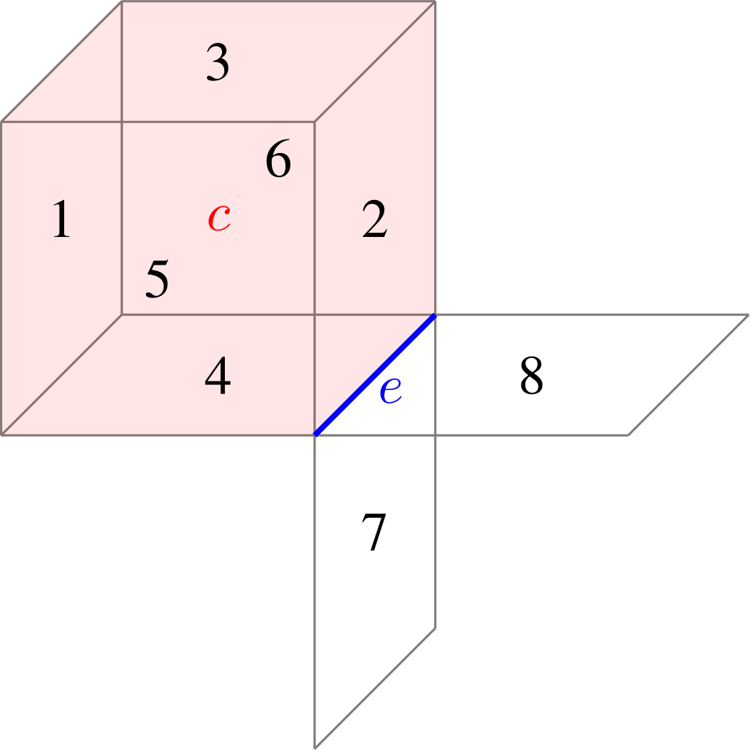
(a)

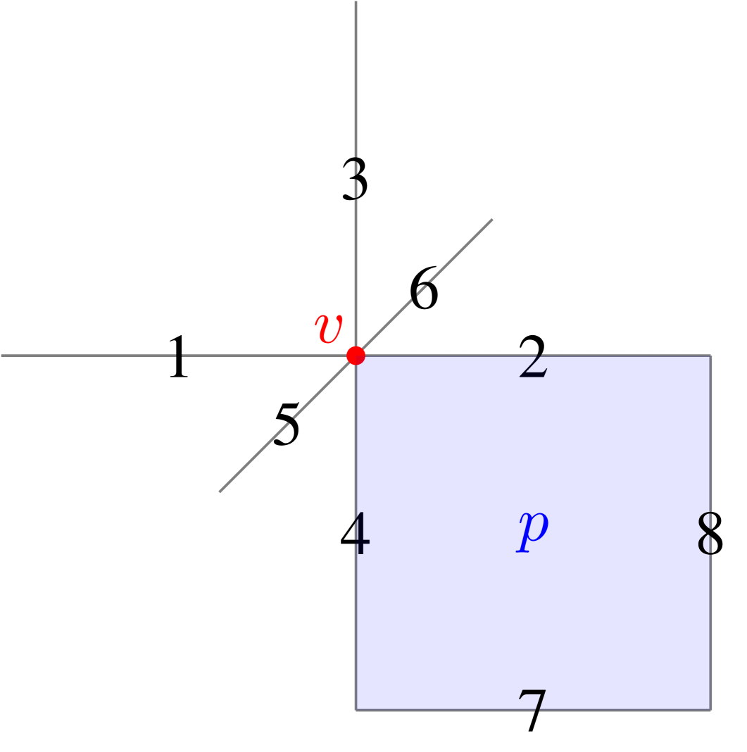
(b)

Figure 5: Illustration of $A$ term and $B$ term of 3-dimensional toric code under two conventions. (a) The first convention, where spins are on plaquettes. The $A$ term supported on cube $c$ is $A_{c}=X_{1}X_{2}X_{3}X_{4}X_{5}X_{6}$. The $B$ term supported on edge $e$ is $B_{e}=Z_{2}Z_{4}Z_{7}Z_{8}$. (b) The second convention, where spins are on edges. The $A$ term supported on vertex $v$ is $A_{v}=X_{1}X_{2}X_{3}X_{4}X_{5}X_{6}$. The $B$ term supported on plaquette $p$ is $B_{p}=Z_{2}Z_{4}Z_{7}Z_{8}$. The first convention is unified in TD models as the $[1,2,3,3]$ model.

These conventions are related by lattice duality, exchanging dimensions and codimensions. The plaquette-centered formulation corresponds to $[1,2,3,3]$ through:

• $d_{n}=1$: $B$ terms attached to 1-dimensional edges

• $d_{s}=2$: Qubits on 2-dimensional plaquettes

• $d_{l}=3$: $B$ terms span 3-dimensional leaves

• $D=3$: $A$ terms on 3-cubes $\&$ Lattice dimension

The ground state degeneracy under periodic boundary condition is $\text{GSD}=8$, encoding 3 logical qubits. Key features include:

• Excitations:

  • Point-like $e$ particles from string operators

  • Extended $m$-loops from membrane operators

• Dimensional hierarchy:

  • $e$ particles created at string endpoints

  • $m$-loops energy $\propto$ perimeter

II.3.5 $[1,2,3,4]$ model

The $[1,2,3,4]$ model is a 4-dimensional fracton ordered model [23], defined on a 4-dimensional hypercubic lattice where each plaquette hosts a $\frac{1}{2}$-spin. The Hamiltonian is

$$H =-\sum_{\gamma_{4}}A_{\gamma_{4}}-\sum_{\gamma_{1}}\sum_{l\mathchoice{\rotatebox[origin={c}]{180.0}{$\subset$}}{\rotatebox[origin={c}]{180.0}{$\subset$}}{\rotatebox[origin={c}]{180.0}{$\scriptstyle\subset$}}{\rotatebox[origin={c}]{180.0}{$\scriptscriptstyle\subset$}}\gamma_{1}}B_{\gamma_{1},l}\,,$$ (11)

where $A_{\gamma_{4}}=\prod_{\gamma_{2}\subset\gamma_{4}}X_{\gamma_{2}}$, and $B_{\gamma_{1},l}$ is the product of Pauli $Z$ operators of four nearest spins to $\gamma_{1}$ in leaf $l$. The $A$ and $B$ terms are illustrated in Fig. 6

(a) $A_{\gamma_{4}}=X_{1}X_{2}\cdots X_{24}$.

(b)

Figure 6: Illustration of $A$ term and $B$ term in the $[1,2,3,4]$ model. The spins are on plaquettes, and the numbers in this figure are placed at the center of each plaquette, representing the spin on it. (a) The $A$ term associated with 4-cube $\gamma_{4}$ is $A_{\gamma_{4}}=X_{1}X_{2}\cdots X_{24}$, supported by all the plaquettes in $\gamma_{4}$. The dashed cube aids visualizing plaquettes spanning in $x_{4}$-direction: the centers of plaquettes spanning in $x_{4}$-direction coincide with the centers of edges of the dashed cube. (b) Each $B$ term attached to edge $e$ is supported by 4 plaquettes containing $e$, e.g. $B_{e,x_{1}x_{2}x_{3}}=Z_{1}Z_{2}Z_{3}Z_{4}$, $B_{e,x_{1}x_{3}x_{4}}=Z_{1}Z_{2}Z_{5}Z_{6}$ There are 3 $B$ terms attached to $e$ in due to the combinatorial factor $C_{D-d_{n}}^{d_{l}-d_{n}}=C_{4-1}^{3-1}=3$, which are $B_{e,x_{1}x_{2}x_{3}},B_{e,x_{1}x_{2}x_{4}},B_{e,x_{1}x_{3}x_{4}}$.

For each $\gamma_{1}$, there are $C_{D-d_{n}}^{d_{l}-d_{n}}=C_{4-1}^{3-1}=3$ different $B_{\gamma_{1},l}$ attached to it. The GSD of $[1,2,3,4]$ model satisfies $\log_{2}GSD=3(L_{1}+L_{2}+L_{3}+L_{4})-6$ under PBC for a lattice of size $L_{1}\times L_{2}\times L_{3}\times L_{4}$ [24], encoding $3(L_{1}+L_{2}+L_{3}+L_{4})-6$ logical qubits.

There are two fundamental excitation types in the $[1,2,3,4]$ model, associated with the $A$-term and $B$-term respectively. Applying a Pauli $Z$ operator on a dual lattice rectangular membrane creates four $A_{\gamma_{4}}=-1$ excitations at the four corners of the rectangular membrane. The $A_{\gamma_{4}}=-1$ excitations cannot move independently, thus are fractons. Two nearby $A_{\gamma_{4}}=-1$ fractons combine to form a “volumeon” that is mobile within a 3-dimensional leaf.

Applying a Pauli $Z$ operator on an open flat membrane creates an $m$-string excitation along the membrane’s perimeter, where the energy distributes uniformly. Intriguingly, a curved membrane creates additional string-like excitations along its crease lines, which prevent loop-like excitations from moving or deforming freely. This phenomenon indicates that curved membranes generate non-manifold-like excitations, collectively referred to as “complex excitations” in Ref. [23].

II.3.6 $[2,3,4,4]$ model as a 4-dimensional Toric Code

The $[2,3,4,4]$ model represents a 4-dimensional pure topological order, serving as a $(1,3)$-type 4-dimensional Toric Code with 1-dimensional $Z$-type and 3-dimensional $X$-type logical operators. While not unique among 4-dimensional Toric Codes - other variants include $(2,2)$-type [141] and octaplex-tessellated models [142] - its Hamiltonian on a 4-dimensional hypercubic lattice (qubits on 3-cubes) is:

$$H =-\sum_{\gamma_{4}}A_{\gamma_{4}}-\sum_{\gamma_{2}}B_{\gamma_{2}}$$

$$=-\sum_{\gamma_{4}}\prod_{\gamma_{3}\subset\gamma_{4}}X_{\gamma_{3}}-\sum_{\gamma_{2}}\prod_{\gamma_{3}\supset\gamma_{2}}Z_{\gamma_{3}}\,.$$ (12)

Like 2-dimensional Toric Code and 3-dimensional Toric Code, the only existing leaf $l$ contains the whole lattice, so the index $l$ is neglected. As an $(1,3)$-type 4-dimensional Toric Code model, in $[2,3,4,4]$ model we have two kinds of logical operators which are respectively 1-dimensional and 3-dimensional. An 1-dimensional logical operator here is the product of Pauli $Z$ on cubes along a non-contractible dual string $S^{1}$, and a 3-dimensional logical operator here is the product of Pauli $X$ on cubes along a 3-dimensional torus $T^{3}$. By counting the number of independent logical operators, we can obtain that under PBC the GSD of $[2,3,4,4]$ is 16 encoding $4$ logical qubits.

There are two kinds of fundamental excitation in the $[2,3,4,4]$ model, associated with $A$ term and $B$ term respectively. Applying Pauli $Z$ on an open dual string on a ground state creates two $A_{\gamma_{4}}=-1$ excitations on the two ends of the dual string. Two $A_{\gamma_{4}}=-1$ excitations fuse to vacuum. Applying Pauli $X$ on an open 3-dimensional region creates a closed membrane excitation on the boundary of the region. Along the entire closed membrane, $B_{\gamma_{2}}=-1$, the energy of the closed membrane excitation is proportional to the area of the membrane, in which sense it is called a spatially extended topological excitation.

II.4 Hierarchy of long-range entanglement, nested leaf Structure, and ground state degeneracy

It is generally established that topological orders are distinguished by their nontrivial long-range entanglement (LRE) patterns, with fracton orders exhibiting complex LRE structures under entanglement renormalization group (ERG) transformations [21, 143, 22]. The X-cube model ($[0,1,2,3]$) serves as a fixed point under ERG transformations, which involve two key steps: first, inserting layers of 2-dimensional Toric Code ($[0,1,2,2]$) ground states into the cubic lattice, followed by application of finite-depth local unitary (LU) circuits. A hierarchical classification framework of long range entanglement (LRE) for TD models has been established [22], organizing these models into distinct levels where lower-level TD states function as building blocks in ERG transformations of higher-level counterparts. Specifically:

• Level-0: Short-range entangled states or disentangled product states

• Level-1: $[0,1,2,2]$ ground states requiring spin-line insertion/removal in product states

• Level-2: $[0,1,2,3]$ ground states involving membrane insertion/removal of level-1 states

This hierarchy generalizes through the relation $[d-1,d,d+1,D]\rightarrow\text{level-}(D-d)$ LRE states [22], extending foliated fracton theory. For instance, 3-dimensional leaves added/removed in the ERG of $[0,1,2,4]$ model are in $[0,1,2,3]$ ground states, which also has a leaf structure under ERG with LRE states on the leaves. Such nested leaf architectures distinguish general TD models from conventional 3-dimensional foliated fracton systems. The hierarchical structure of ERG among TD states with different LRE-levels suggests LRE-level quantifies LRE complexity.

Analogous to the Toric Code, any TD model exhibits unique ground state under open boundary condition (OBC), while demonstrating nontrivial ground state degeneracy (GSD) under PBC. Reference [24] quantifies the GSD for two classes of these models: level-1 TD models display constant GSD under PBC, whereas higher-level counterparts exhibit $\log_{2}\mathrm{GSD}$ scaling polynomially with system size under equivalent boundary conditions.

II.5 Non-stabilizer-code TD models: A pathway to transverse field Ising models and beyond

We briefly discuss TD models that are not stabilizer codes, where $A$ and $B$ terms are non-commuting. These models exhibit interesting properties in the context of (quantum) statistical physics. The 1-dimensional transverse field Ising model serves as prototype $[0,1,1,1]$ TD model with edge spins:

$$H=-\sum_{e}A_{e}-\sum_{v}B_{v}=-\sum_{e}X_{e}-\sum_{v}\prod_{e\supset v}Z_{e}.$$ (13)

For general cases with $d_{n}=d_{s}=d_{l}$, the Hamiltonian reduces to transverse field Ising-type:

$$B_{\gamma_{d_{n}}}=Z_{\gamma_{d_{n}}}=Z_{\gamma_{d_{s}}},$$

yielding non-stabilizer codes. Notable examples include:

• $[0,0,0,2]$ and $[1,1,1,2]$: Transverse field plaquette Ising models

• $[0,0,0,3]$: Transverse field cubic Ising model

Non-stabilizer TD models exhibit rich critical behavior. The paradigmatic 1-dimension transverse-field Ising model with tunable parameters:

$$H=-h\sum_{e}A_{e}-J\sum_{v}B_{v}=-h\sum_{e}X_{e}-J\sum_{v}\prod_{e\supset v}Z_{e}$$ (14)

shows a critical line at $h=J$ with gapless CFT description [144, 145], $\mathbb{Z}_{2}$-symmetric phase ($h>J$) and symmetry-broken phase ($h<J$). Key open questions include: existence of critical lines/intermediate phases in general non-stabilizer TD models, ERG connections between different critical systems, and universality class classification for higher-dimensional analogs. These directions represent promising avenues for exploring non-stabilizer TD model phenomenology.

III Sequential quantum circuit for preparing TD models

For simplicity, we denote $d_{s}$ by $d$ throughout this section. Given any stabilizer code TD model $[d_{n},d,d_{l},D]$ under OBC, PBC, or half-OBC-half-PBC, a ground state is expressed as:

$$c\prod_{\text{all }\gamma_{D}}\left(1+A_{\gamma_{D}}\right)|00\cdots 0\rangle\,,$$ (15)

where $c$ is the normalization factor, which is explicitly calculated in appendix B. In this section, we provide a SQC for preparing such a ground state of any stabilizer code TD model, i.e. a SQC mapping the initial state $|00\cdots 0\rangle$, where $|0\rangle:=|Z=1\rangle$, to Eq. (15). Our SQC is applicable to OBC, PBC, and half-OBC-half-PBC: while the SQC for PBC consists of $d+1$ mutually non-commutable steps, the first step prepares the TD state under OBC, and the SQC for half-OBC-half-PBC can be obtained by truncating the SQC. Therefore, we focus on SQC for PBC first, and after introducing the unified SQC for any stabilizer code TD model, we show how to truncate the SQC to obtain the SQC for half-OBC-half-PBC. From now on, if not specified, we discuss the SQC for PBC by default.

The overall strategy of our SQC is:

1. Prepare the system in the initial state $|00\cdots 0\rangle$.
   

2. Choose a set of $\gamma_{D}$, denoted by $\Gamma_{D}\backslash R_{D}$, which supports a minimal complete set of $A$ terms. $\Gamma_{D}$ is the set of all $\gamma_{D}$ in lattice, and $R_{D}\subset\Gamma_{D}$. The choice of $R_{D}$ is model dependent, and will be discussed in detail later.
   

3. Choose a representative spin (or $\gamma_{d}$) in each $\gamma_{D}\in\Gamma_{D}\backslash R_{D}$, such that there is a one-to-one correspondence between representative spin and $\gamma_{D}\in\Gamma_{D}\backslash R_{D}$. Apply Hadamard gates on all representative spins.
   

4. Apply CNOT gates, with the representative spins being control qubits, and all other spins in the represented $\gamma_{D}$ being target qubits, in an order that no representative spin plays the role of target qubit before it has finished playing the role of control qubit.

The readers may wonder why not choosing a representative spin in every $\gamma_{D}$ and apply CNOT gates, which seems much more straightforward. The answer is under PBC, this is impossible: whether the constraint of order stated in the overall strategy would be broken, or if one does it anyway, the result state will not be a ground state. We will see the reason soon, in the first example.

How arbitrary can $\Gamma_{D}\backslash R_{D}$ and representative spins be chosen is not studied in this paper, instead, we provide a concrete scheme. In our scheme, the first layer is the Hadamard gates, applied to all the representative spins. We call the first layer step 0, for convenience. Apart from the Hadamard gates, the SQC for preparing $[d_{n},d,d_{l},D]$ model ground state consists of $d+1$ steps, which are mutually non-commutable, labeled by step 1,2,$\cdots,d+1$. Step $k+1$ has $C_{D}^{k}$ mutually commutable parts, which can be applied simultaneously. The concrete form of any part of any step of the SQC will be presented in the rest of this section, starting from concrete examples. While the examples show useful step-by-step details, the readers who want to know the unified formal formula may directly jump to Sec. III.5 as well as the supplemented materials in Appendix B.

III.1 $[0,1,2,2]$ model

As illustrated in Sec. II, the $[0,1,2,2]$ model is Toric Code (on square lattice). In this subsection, we construct a SQC for preparing the $[0,1,2,2]$ model, where $d=1,D=2$. We start from graphic illustration, then algebraically write the SQC, find a stabilizer redundancy, by using which we show the equal weight superposition of configurations on all plaquettes exist in the final state, explicitly or implicitly.

Let us start with the graphic illustration. Consider a $4\times 4$ square lattice under PBC, where each edge has a $\frac{1}{2}$-spin on it. Prepare the system in product state $|00\cdots 0\rangle$, where $|0\rangle=|Z=1\rangle$ is a Pauli $Z$ eigenstate. Then, apply Hadamard gates to each spin on orange edges shown below:

$$\leavevmode\hbox to143.24pt{\vbox to142.04pt{\text{[drawing]}}}\ , x_{1} x_{2}$$ (16)

after which the spins on orange lines are in state $|+\rangle=|X=1\rangle$. Those orange edges are the representative spins in the overall strategy. From now on, we use black edges to represent spins in state $|0\rangle$, and orange edges to represent spins in state $|+\rangle$ in this subsection. For simplicity, we call the application of the Hadamard gates step 0 of the SQC. After step 0, apply $d+1=2$ non-commutable steps of CNOT gates, namely, step 1 and step 2, which shall be applied with the order 1,2. Denote

$$\leavevmode\hbox to29.45pt{\vbox to29.45pt{\text{[drawing]}}}\ =\ \leavevmode\hbox to29.45pt{\vbox to29.15pt{\text{[drawing]}}}$$ (17)

On the left hand side of Eq. (17), each arrow represents a CNOT gate, with the tail being the control qubit, and the head being the target qubit. The right hand side of Eq. (17) is just a symbolic simplification. Step 1 and step 2 are:

• Step 1 (consisting of $C_{2}^{0}=1$ part):

  $$\leavevmode\hbox to143.24pt{\vbox to142.04pt{\text{[drawing]}}}\ , x_{1} x_{2}$$ (18)

  where the numbers label the layers, i.e. gates labeled by the same number are mutually commutable, and are applied simultaneously; gates labeled by smaller number are applied first, then follow the gates with larger numbers.

• Step 2 consists of $C_{2}^{1}=2$ mutually commutable parts, denoted by part $\{1\}$ and part $\{2\}$. The reason for using a set to denote a part is that a set of $k$ distinct numbers in $\{1:D\}:=\{1,2,\cdots,D\}$ has exactly $C_{D}^{k}$ possibilities, which perfectly labels the $C_{D}^{k}$ mutually commutable parts of step $k+1$. Later, when the SQC is written algebraically, it will be easily seen the set $S_{k}$ labeling a part has a clear meaning.

  • Step 2 part $\{1\}$:

    $$\leavevmode\hbox to143.24pt{\vbox to142.04pt{\text{[drawing]}}}\ . x_{1} x_{2}$$ (19)

  • Step 2 part $\{2\}$:

    $$\leavevmode\hbox to143.24pt{\vbox to142.04pt{\text{[drawing]}}}\ . x_{1} x_{2}$$ (20)

  Step 2 part $\{1\}$ and step 2 part $\{2\}$ are mutually commutable, thus can be applied simultaneously. Step 2 must be applied after step 1.

The two steps create the equal weight superposition of configurations (EWSCs) on all plaquettes, except the one on the right top corner. However, the missed configuration is implicitly created out of $A$ term stabilizer redundancy, which we explain in this subsection soon. In this example, the plaquette on the right top corner itself consists the plaquette set $R_{D}$ mentioned in the overall strategy.

To give precise description of why the EWSC on the right top corner plaquette implicitly exists, writing the SQC algebraically is necessary. Let us first represent specific $n$-cubes algebraically, and then write the SQC. For any dimensional cubical lattice, the geometric center of $\gamma_{n}$ has a one to one correspondence with $\gamma_{n}$, no matter what $n$, thus we can use the coordinates of geometric center to represent $\gamma_{n}$. Take the lattice constant to be 1, and some vertex to be at $(0,0,\cdots,0)$, the coordinates of $\gamma_{n}$’s geometric center $(x_{1},x_{2},\cdots,x_{D})$ will contain $n$ half-integers and $(D-n)$ integers. Use the coordinates of geometric center to represent any $\gamma_{n}$,

$$\gamma_{n}\Big{(}\text{center at }(x_{1},x_{2},\cdots,x_{D})\Big{)}:=[x_{1},x_{2},\cdots,x_{D}]\,.$$ (21)

According to Eq. (21), we can use for example $[2,3]$ to represent the vertex at $(2,3)$, $[5,3+\frac{1}{2}]$ to represent the edge whose center is at $(5,3+\frac{1}{2})$, $[\frac{1}{2},L_{2}-\frac{3}{2}]$ to represent the plaquette whose center is at $(\frac{1}{2},L_{2}-\frac{3}{2})$. Using this notation, we can write the SQC in this subsection as following:

The initial state is still $|00\cdots 0\rangle$. The state after step 0 is:

$$\begin{split}&\Bigg{(}\prod_{\begin{subarray}{c}x_{1}\in\mathbb{Z}_{L_{1}-1}\\ x_{2}\in\mathbb{Z}_{L_{2}-1}\end{subarray}}\text{Had}_{[x_{1},x_{2}+\frac{1}{2}]}\Bigg{)}\Bigg{(}\prod_{x_{2}\in\mathbb{Z}_{L_{2}-1}}\text{Had}_{[-\frac{1}{2},x_{2}]}\Bigg{)}\\ &\quad\quad\quad\quad\quad\quad\quad\Bigg{(}\prod_{x_{1}\in\mathbb{Z}_{L_{1}-1}}\text{Had}_{[x_{1},-\frac{1}{2}]}\Bigg{)}|00\cdots 0\rangle\,,\end{split}$$ (22)

where $L_{1},L_{2}$ are length of the lattice in $x_{1},x_{2}$-directions, respectively. The huge parentheses are added here to restrict the effective range of indices under $\sum$, i.e. ($x_{1},x_{2}$). $\mathbb{Z}_{N}:=\{0,1,\cdots,N-1\}$ is the $N$-th order cyclic group.

$$x_{i}=x_{i}\ \text{mod}\ L_{i}$$ (23)

is applied because of PBC.
Step 1:

$$\prod_{n=0}^{L_{1}-2}\prod_{\begin{subarray}{c}x_{i}\in\mathbb{Z}_{L_{i}-1},\,i=1,2\\ x_{1}=n\end{subarray}}\prod_{\begin{subarray}{c}\gamma_{1}\subset[x_{1}+\frac{1}{2},x_{2}+\frac{1}{2}]\\ \gamma_{1}\neq[x_{1},x_{2}+\frac{1}{2}]\end{subarray}}\text{CNOT}_{[x_{1},x_{2}+\frac{1}{2}],\gamma_{1}}\,.$$ (24)

The readers may feel confused at the first glance to the conditions under the second $\prod$ in Eq. (24): $x_{1}\in\mathbb{Z}_{L_{1}-1}$ can be derived from $x_{1}=n$, why writing the redundant condition $x_{1}\in\mathbb{Z}_{L_{1}-1}$? The answer is to be consistent with the unified form of SQC. Just like all other $\prod$ with multi-conditions, only the indices satisfying all conditions under $\prod$ is taken to support the product. Also, be careful that for any set of operators $\{O_{i}\}$, $\prod_{n=0}^{L_{1}-2}O_{n}:=O_{0}O_{1}\cdots O_{L_{1}-2}$ has $O_{L_{1}-2}$ on the right most, which is the layer 1, and $O_{0}$ on the left most, being the last layer. Step 1 creates the EWSCs on all the plaquettes with no coordinate being $-\frac{1}{2}$.
Step 2 part $\{1\}$:

$$\prod_{n=0}^{L_{2}-2}\prod_{\begin{subarray}{c}x_{2}=n\end{subarray}}\,\prod_{\begin{subarray}{c}\gamma_{1}\subset[-\frac{1}{2},x_{2}+\frac{1}{2}]\\ \gamma_{1}\neq[-\frac{1}{2},x_{2}]\end{subarray}}\text{CNOT}_{[-\frac{1}{2},x_{2}],\gamma_{1}}\,.$$ (25)

Step 2 part $\{1\}$ creates the EWSCs on plaquettes with only $x_{1}$ but no other coordinate being $-\frac{1}{2}$.
Step 2 part $\{2\}$:

$$\prod_{n=0}^{L_{1}-2}\prod_{\begin{subarray}{c}x_{1}=n\end{subarray}}\,\prod_{\begin{subarray}{c}\gamma_{1}\subset[x_{1}+\frac{1}{2},-\frac{1}{2}]\\ \gamma_{1}\neq[x_{1},-\frac{1}{2}]\end{subarray}}\text{CNOT}_{[x_{1},-\frac{1}{2}],\gamma_{1}},.$$ (26)

Step 2 part $\{2\}$ creates the EWSCs on plaquettes with only $x_{2}$ but no other coordinate being $-\frac{1}{2}$.
Step 2 creates the EWSCs on all the plaquettes with exactly 1 coordinate being $-\frac{1}{2}$.

The state after applying the SQC is

$$\begin{split}&\Bigg{(}\prod_{x_{i}\in\mathbb{Z}_{L_{i}-1},\,i=1,2}\frac{1}{\sqrt{2}}\Big{(}1+A_{[x_{i}+\frac{1}{2}|i=1,2]}\Big{)}\Bigg{)}\\ &\Bigg{(}\prod_{x_{2}\in\mathbb{Z}_{L_{2}-1}}\frac{1}{\sqrt{2}}\Big{(}1+A_{[-\frac{1}{2},x_{2}+\frac{1}{2}]}\Big{)}\Bigg{)}\\ &\Bigg{(}\prod_{x_{1}\in\mathbb{Z}_{L_{1}-1}}\frac{1}{\sqrt{2}}\Big{(}1+A_{[x_{1}+\frac{1}{2},-\frac{1}{2}]}\Big{)}\Bigg{)}|00\cdots 0\rangle\,,\end{split}$$ (27)

this result is a special case of Eq. (168), derived in appendix B.

Under PBC, there is a redundant $A$ term in Hamiltonian, i.e. there is a $A_{p}$ term, which is the multiplication of other $A_{p}$ terms, so that the ground space is invariant under deleting or adding that $A_{p}$ term into Hamiltonian. We define such an equation

$$A_{p^{\prime}}=\prod_{p\in\xi}A_{p},\quad p^{\prime}\notin\xi$$ (28)

as an $A$ term redundancy, as a type of stabilizer redundancy. The $A_{p}$ term on the plaquette $[-\frac{1}{2},-\frac{1}{2}]$ equals to the multiplication of all other $A_{p}$ terms. Denote the set of all plaquettes as $\mathscr{P}$, the $A$ term redundancy is

$$A_{[-\frac{1}{2},-\frac{1}{2}]}=\prod_{p\in\mathscr{P}\backslash[-\frac{1}{2},-\frac{1}{2}]}A_{p}\,.$$ (29)

Note that EWSCs on all plaquettes, except $[-\frac{1}{2},-\frac{1}{2}]$, explicitly appear in Eq. (27), so Eq. (27) can be written as

$$\prod_{p\in\mathscr{P}\backslash[-\frac{1}{2},-\frac{1}{2}]}\frac{1}{\sqrt{2}}\Big{(}1+A_{p}\Big{)}|00\cdots 0\rangle\,.$$

Using Eq. (29), we can write

$$A_{[-\frac{1}{2},-\frac{1}{2}]}\prod_{p\in\mathscr{P}\backslash[-\frac{1}{2},-\frac{1}{2}]}\frac{1}{\sqrt{2}}\Big{(}1+A_{p}\Big{)}$$

$$= \prod_{p\in\mathscr{P}\backslash[-\frac{1}{2},-\frac{1}{2}]}A_{p}\frac{1}{\sqrt{2}}\Big{(}1+A_{p}\Big{)}$$

$$= \prod_{p\in\mathscr{P}\backslash[-\frac{1}{2},-\frac{1}{2}]}\frac{1}{\sqrt{2}}\Big{(}1+A_{p}\Big{)}\,,$$ (30)

thus Eq. (27.1) equals to

$$\begin{split}&\frac{1}{2}\Big{(}1+A_{[-\frac{1}{2},-\frac{1}{2}]}\Big{)}\prod_{p\in\mathscr{P}\backslash[-\frac{1}{2},-\frac{1}{2}]}\frac{1}{\sqrt{2}}\Big{(}1+A_{p}\Big{)}|00\cdots 0\rangle\\ &=\frac{1}{\sqrt{2}}\prod_{p\in\mathscr{P}}\frac{1}{\sqrt{2}}\Big{(}1+A_{p}\Big{)}|00\cdots 0\rangle\,,\end{split}$$

which is a ground state of 2-dimensional Toric Code, since for any $A_{p^{\prime}},B_{v^{\prime}}$,

$$A_{p^{\prime}}\prod_{p\in\mathscr{P}}\Big{(}1+A_{p}\Big{)}|00\cdots 0\rangle=\prod_{p\in\mathscr{P}}\Big{(}1+A_{p}\Big{)}|00\cdots 0\rangle\,,$$ (31)

$$\begin{split}B_{v^{\prime}}\prod_{p\in\mathscr{P}}\Big{(}1+A_{p}\Big{)}|00\cdots 0\rangle&=\prod_{p\in\mathscr{P}}\Big{(}1+A_{p}\Big{)}B_{v^{\prime}}|00\cdots 0\rangle\\ &=\prod_{p\in\mathscr{P}}\Big{(}1+A_{p}\Big{)}|00\cdots 0\rangle\,,\end{split}$$ (32)

and the eigenvalues of $A_{p^{\prime}},B_{v^{\prime}}$ can only be $\pm 1$. Note that the convention is $B_{v}=\prod_{e\mathchoice{\rotatebox[origin={c}]{180.0}{$\subset$}}{\rotatebox[origin={c}]{180.0}{$\subset$}}{\rotatebox[origin={c}]{180.0}{$\scriptstyle\subset$}}{\rotatebox[origin={c}]{180.0}{$\scriptscriptstyle\subset$}}v}Z_{e}$.

Finally, it is worthy noting that after the SQC, further applying Hadamard and CNOT gates inside the right top plaquette or the plaquette $\left[-\frac{1}{2},-\frac{1}{2}\right]$ would make the state no longer a Toric Code ground state. The existence of such a plaquette is topological, since it is directly related to the $A$ term redundancy, which exists on $T^{2}$ (i.e. under PBC), and does not exist on $B^{2}$ (i.e. under OBC) or $T^{1}\times B^{1}$ (i.e. under hybrid half-PBC-half-OBC).

III.2 $[0,1,2,3]$ model

As illustrated in Sec. II, the $[0,1,2,3]$ model is X-cube (on cubic lattice). In this subsection, we construct a SQC for preparing the $[0,1,2,3]$ model, where $d=1,D=3$. Again, we start from graphic illustration, then algebraically write the SQC, find a set of stabilizer redundancies, by using which we show the equal weight superposition of configurations on all cubes exist in the final state, explicitly or implicitly. Unlike the $[0,1,2,2]$ model, which has only one $A$ term redundancy equivalent class, the $[0,1,2,3]$ model has multiple $A$ term redundancy classes with intersecting structure, which we will discuss soon.

Let us start with the graphic illustration again. Consider a $2\times 3\times 3$ cubic lattice under PBC, where each edge has a $\frac{1}{2}$-spin on it. Prepare the system in product state $|00\cdots 0\rangle$, where $|0\rangle=|Z=1\rangle$ is a Pauli $Z$ eigenstate. Then, apply Hadamard gates to each spin on orange edges shown below:

$$\leavevmode\hbox to152.2pt{\vbox to108.27pt{\text{[drawing]}}}\ , x_{1} x_{2} x_{3}$$ (33)

after which the spins on orange lines are in state $|+\rangle=|X=1\rangle$. The spins on those orange lines are the representative spins in the overall strategy. From now on, we use black edges to represent spins in state $|0\rangle$, and orange edges in state $|+\rangle$ in this subsection. Again, we call the application of the Hadamard gates step 0 of the SQC. After step 0, apply $d+1=2$ non-commutable steps of CNOT gates, namely, step 1 and step 2, which shall be applied with the order 1,2. Denote

$$\leavevmode\hbox to40.41pt{\vbox to40.41pt{\text{[drawing]}}}\ =\ \leavevmode\hbox to40.11pt{\vbox to40.11pt{\text{[drawing]}}}\ .$$ (34)

On the left hand side of Eq. (34), each arrow represents a CNOT gate, as before, and the right hand side is just a symbolic simplification. Step 1 is:

• Step 1 (consisting of $C_{3}^{0}=1$ part):

  $$\leavevmode\hbox to151.9pt{\vbox to107.67pt{\text{[drawing]}}}\ . x_{1} x_{2} x_{3}$$ (35)

Note that in Eq. (35), we do not draw the orange lines that are not involved in step 1, for visual clearness. The number labels different layers, as before. Unfortunately, a $2\times 3\times 3$ lattice is not large enough to display the full pattern of step 1, but a larger 3-dimensional figure is not friendly to read, so we draw a projective 2-dimensional figure below:

$$\leavevmode\hbox to169.97pt{\vbox to140.32pt{\text{[drawing]}}}\ . x_{1} x_{2} x_{3}$$ (36)

The figure in Eq. (36) should be recognized as the top view of Eq. (35) from $x_{3}$-direction, with larger $L_{1},L_{2}$.

If OBC is applied, step 1 is enough to create a ground state of X-cube. Under PBC, where GSD is not one, additional circuit, i.e. step 2, needs to be applied. Step 2 is:

• Step 2 consists of $C_{3}^{1}=3$ mutually commutable parts, denoted by parts $\{1\},\{2\},\{3\}$.

  • Step 2 part $\{1\}$ (following Eq. (35)):

    $$\leavevmode\hbox to151.9pt{\vbox to107.97pt{\text{[drawing]}}}\ . x_{1} x_{2} x_{3}$$ (37)

  • Step 2 part $\{2\}$:

    $$\leavevmode\hbox to152.2pt{\vbox to107.67pt{\text{[drawing]}}}\ . x_{1} x_{2} x_{3}$$ (38)

  • Step 2 part $\{3\}$:

    $$\leavevmode\hbox to151.9pt{\vbox to107.97pt{\text{[drawing]}}}\ . x_{1} x_{2} x_{3}$$ (39)

    Like for step 1, we do not draw the orange lines that are not involved in present part of step 2, for visual clearness. The number labels different layers, as before. Again, a $2\times 3\times 3$ lattice is not large enough to display the full pattern of parts $\{2\},\{3\}$ of step 2, but parts $\{1\},\{2\},\{3\}$ have the same pattern, so the full pattern of parts $\{2\},\{3\}$ can be inferred. Different parts of step 2 are mutually commutable, thus can be applied simultaneously.

The two steps create EWSCs on all cubes, except the red cubes $c_{1},c_{2},c_{3},c_{4},c_{5},c_{6}$ shown below:

$$\includegraphics[width=130.08731pt]{paper_X-cube_3.pdf}\ .$$ (40)

Denote the set of all $\gamma_{3}$(cubes) by $\Gamma_{3}$, and the set of all $\gamma_{3}$, on which the EWSCs are not explicitly created by the SQC, by $R_{3}$. Under the setting of Eq. (40), $R_{3}=\{c_{1},c_{2},c_{3},c_{4},c_{5},c_{6}\}$. The state after applying steps 1,2 is

$$\prod_{c\in\Gamma_{3}\backslash R_{3}}\frac{1}{\sqrt{2}}\Big{(}1+A_{c}\Big{)}|00\cdots 0\rangle\,.$$ (41)

Again, we describe this SQC algebraically, and then discuss how the EWSCs on $R_{3}$ implicitly exist in Eq. (41), out of stabilizer redundancy.

The initial state is $|00\cdots 0\rangle$. Then we apply Hadamard gates on representative spins (step 0), after which the state becomes

$$\begin{split}&\Bigg{(}\prod_{x_{i}\in\mathbb{Z}_{L_{i}-1},\,i=1,2,3}\text{Had}_{[x_{1},x_{2},x_{3}+\frac{1}{2}]}\Bigg{)}\\ &\Bigg{(}\prod_{j=1}^{3}\ \prod_{x_{i}\in\mathbb{Z}_{L_{i}-1},\,i\neq j}\text{Had}_{[-\frac{1}{2},x_{i}|i\neq j]}\Bigg{)}|00\cdots 0\rangle\,,\end{split}$$ (42)

where the subscript $[-\frac{1}{2},x_{i}|i\neq j]$ stands for $[-\frac{1}{2},x_{2},x_{3}]$ when $j=1$, $[x_{1},-\frac{1}{2},x_{3}]$ when $j=2$, and $[x_{1},x_{2},-\frac{1}{2}]$ when $j=3$.

Define a symbol called group CNOT to simplify the formula:

$$\text{GCNOT}_{s}^{\xi}:=\prod_{s^{\prime}\in(\xi\backslash\{s\})}\text{CNOT}_{s,s^{\prime}}\,,$$ (43)

i.e. the product of CNOT gates with the same control qubit $s$, and a set of target qubits $\xi\backslash\{s\}$. The control qubit is automatically excluded from the target qubits set, to meet with the definition of CNOT gate as a two qubit operation. Note that the CNOT gates with the same control qubit are commutable, group CNOT just collect some of those commutable CNOT gates by multiplying them together. The idea is to represent the CNOT gates inside the same cube as a whole.
Step 1:

$$\prod_{n=0}^{\sum_{i=1,2}(L_{i}-2)}\prod_{\begin{subarray}{c}x_{i}\in\mathbb{Z}_{L_{i}-1},\,i=1,2,3\\ \sum_{i=1,2}x_{i}=n\end{subarray}}\text{GCNOT}_{[x_{1},x_{2},x_{3}+\frac{1}{2}]}^{\delta_{d}[x_{i}+\frac{1}{2}|i=1,2,3]}\,,$$ (44)

where

$$\delta_{d}\gamma_{D}:=\big{\{}\gamma_{d}\big{|}\gamma_{d}\subset\gamma_{D}\big{\}}$$ (45)

is the set of all $d$-cubes inside the $\gamma_{D}$. When $d<D$, $\delta_{d}\gamma_{D}$ is the set of all $\gamma_{d}$ on the boundary of corners of $\gamma_{D}$. When $d=D$, $\delta_{d}\gamma_{D}=\{\gamma_{D}\}$. When $d>D$, $\delta_{d}\gamma_{D}=\emptyset$. Step 1 creates the EWSCs on all the plaquettes with 0 coordinate being $-\frac{1}{2}$.
Step 2 part $\{1\}$:

$$\prod_{n=0}^{\sum_{i=2,3}(L_{i}-2)}\prod_{\begin{subarray}{c}x_{i}\in\mathbb{Z}_{L_{i}-1},\,i=2,3\\ \sum_{i=2,3}x_{i}=n\end{subarray}}\text{GCNOT}_{[-\frac{1}{2},x_{2},x_{3}]}^{\delta_{d}[-\frac{1}{2},x_{i}+\frac{1}{2}|i=2,3]}\,,$$ (46)

where $\left[\left.-\frac{1}{2},x_{i}+\frac{1}{2}\right.|i=2,3\right]=\left[-\frac{1}{2},x_{2}+\frac{1}{2},x_{3}+\frac{1}{2}\right]$, which should also be understood as the set of edges/spins in it here, to be consistent with Eq. (43). Step 2 part $\{1\}$ creates the EWSCs on all cubes with $x_{1}$ but no other coordinates being $-\frac{1}{2}$.
Step 2 part $\{2\}$:

$$\prod_{n=0}^{\sum_{i=1,3}(L_{i}-2)}\prod_{\begin{subarray}{c}x_{i}\in\mathbb{Z}_{L_{i}-1},\,i=1,3\\ \sum_{i=1,3}x_{i}=n\end{subarray}}\text{GCNOT}_{[x_{1},-\frac{1}{2},x_{3}]}^{\delta_{d}[-\frac{1}{2},x_{i}+\frac{1}{2}|i=1,3]}\,,$$ (47)

where $\left[\left.-\frac{1}{2},x_{i}+\frac{1}{2}\right|i=1,3\right]=\left[x_{1}+\frac{1}{2},-\frac{1}{2},x_{3}+\frac{1}{2}\right]$. Step 2 part $\{2\}$ creates EWSCs on all cubes with $x_{2}$ but no other coordinates being $-\frac{1}{2}$.
Step 2 part $\{3\}$:

$$\prod_{n=0}^{\sum_{i=1,2}(L_{i}-2)}\prod_{\begin{subarray}{c}x_{i}\in\mathbb{Z}_{L_{i}-1},\,i=1,2\\ \sum_{i=1,2}x_{i}=n\end{subarray}}\text{GCNOT}_{[x_{1},x_{2},-\frac{1}{2}]}^{\delta_{d}[-\frac{1}{2},x_{i}+\frac{1}{2}|i=1,2]}\,,$$ (48)

where $\left[\left.-\frac{1}{2},x_{i}+\frac{1}{2}\right|i=1,2\right]=\left[x_{1}+\frac{1}{2},x_{2}+\frac{1}{2},-\frac{1}{2}\right]$. Step 2 part $\{3\}$ creates EWSCs on all cubes with $x_{3}$ but no other coordinates being $-\frac{1}{2}$. The whole step 2 creates the EWSCs on all the plaquettes with exactly 1 coordinate being $-\frac{1}{2}$.

The state after applying the SQC is

$$\begin{split}&\Bigg{(}\prod_{x_{i}\in\mathbb{Z}_{L_{i}-1},\,i=1,2,3}\frac{1}{\sqrt{2}}\Big{(}1+A_{[x_{i}+\frac{1}{2}|i=1,2,3]}\Big{)}\Bigg{)}\\ &\Bigg{(}\prod_{j=1}^{3}\ \prod_{x_{i}\in\mathbb{Z}_{L_{i}-1},\,i\neq j}\frac{1}{\sqrt{2}}\Big{(}1+A_{[-\frac{1}{2},x_{i}+\frac{1}{2}|i\neq j]}\Big{)}\Bigg{)}|00\cdots 0\rangle\,,\end{split}$$

this result is a special case of Eq. (168), derived in the appendix.

Now we discuss the implicitly existing EWSCs, which exist because of stabilizer redundancies. At the end of Sec. III.1, we wrote a stabilizer redundancy equivalent class, here we define this concept formally. Use the symbol $s$ to represent an arbitrary stabilizer, define an equation of the form

$$r^{1}:\ \prod_{s\in\xi}s=1$$ (49)

as a stabilizer redundancy equivalent class, abbreviated as a red. class. We restrict the discussion with stabilizers satisfying

$$s^{2}=1\quad\&\quad[s,s^{\prime}]=0\,.$$ (50)

The red. class in Eq. (49) is equivalent to $|\xi|$ mutually equivalent stabilizer redundancies. The superscript 1 in $r^{1}$ stands for order 1. We will not talk about higher order red. classes in this paper, a systematic study will be provided in the future. We can write the following $A$ term red. classes of X-cube:

$$r^{1}_{[x_{1}+\frac{1}{2},\cancel{x}_{2},\cancel{x}_{3}]}:\ \prod_{x_{2}\in\mathbb{Z}_{L_{2}}}\prod_{x_{3}\in\mathbb{Z}_{L_{3}}}A_{[x_{i}+\frac{1}{2}]}=1,\ x_{1}\in\mathbb{Z}_{L_{1}}\,,$$

$$r^{1}_{[\cancel{x}_{1},x_{2}+\frac{1}{2},\cancel{x}_{3}]}:\ \prod_{x_{1}\in\mathbb{Z}_{L_{1}}}\prod_{x_{3}\in\mathbb{Z}_{L_{3}}}A_{[x_{i}+\frac{1}{2}]}=1,\ x_{2}\in\mathbb{Z}_{L_{2}}\,,$$

$$r^{1}_{[\cancel{x}_{1},\cancel{x}_{2},x_{3}+\frac{1}{2}]}:\ \prod_{x_{1}\in\mathbb{Z}_{L_{1}}}\prod_{x_{2}\in\mathbb{Z}_{L_{2}}}A_{[x_{i}+\frac{1}{2}]}=1,\ x_{3}\in\mathbb{Z}_{L_{3}}\,,$$ (51)

where $[x_{i}+\frac{1}{2}]$ is an abbreviation for $[x_{i}+\frac{1}{2}|i=1:D]$. There are in total $L_{1}+L_{2}+L_{3}$ red. classes in Eq. (51). The subscript $[x_{1}+\frac{1}{2},\cancel{x}_{2},\cancel{x}_{3}]$ represents the union of all closed 3-cubes with the first coordinate being $x_{1}+\frac{1}{2}$. The slashed $x_{2},x_{3}$ correspond to the two extensive directions of $[x_{1}+\frac{1}{2},\cancel{x}_{2},\cancel{x}_{3}]$. $[\cancel{x}_{1},x_{2}+\frac{1}{2},\cancel{x}_{3}],[\cancel{x}_{1},\cancel{x}_{2},x_{3}+\frac{1}{2}]$ are defined similarly. All other $A$ term red. classes can be generated by multiplying red. classes in Eq. (51).

For concreteness, we keep the setting of Eq. (40), i.e. $L_{1}=2,L_{2}=3,L_{3}=3$. The only $A$ term appearing in $r^{1}_{[\cancel{x}_{1},\frac{1}{2},\cancel{x}_{3}]}$ but not appearing in Eq. (41) is the $A$ term associated with $c_{1}$ drawn in Eq. (40), so based on the same reason as Eqs. (29, 30),

$$\begin{split}&\frac{1}{2}\Big{(}1+A_{c_{1}}\Big{)}\prod_{c\in\Gamma_{3}\backslash R_{3}}\frac{1}{\sqrt{2}}\Big{(}1+A_{c}\Big{)}|00\cdots 0\rangle\\ =&\prod_{c\in\Gamma_{3}\backslash R_{3}}\frac{1}{\sqrt{2}}\Big{(}1+A_{c}\Big{)}|00\cdots 0\rangle\,.\end{split}$$ (52)

The EWSC on $c_{1}$ is implicitly created by the SQC out of the $A$ term redundancy $r^{1}_{[\cancel{x}_{1},\frac{1}{2},\cancel{x}_{3}]}$. Similarly, the EWSC on $c_{2}$ is implicitly created by the SQC out of the $A$ term redundancy $r^{1}_{[\cancel{x}_{1},\frac{3}{2},\cancel{x}_{3}]}$, while $c_{3}$ out of $r^{1}_{[\frac{1}{2},\cancel{x}_{2},\cancel{x}_{3}]}$, $c_{4}$ out of $r^{1}_{[\cancel{x}_{1},\cancel{x}_{2},\frac{1}{2}]}$, $c_{5}$ out of $r^{1}_{[\cancel{x}_{1},\cancel{x}_{2},\frac{3}{2}]}$. Therefore,

$$\begin{split}&\prod_{c\in\Gamma_{3}\backslash R_{3}}\frac{1}{\sqrt{2}}\Big{(}1+A_{c}\Big{)}|00\cdots 0\rangle\\ =&\prod_{i=1,2,\cdots,5}\frac{1}{2}\Big{(}1+A_{c_{i}}\Big{)}\prod_{c\in\Gamma_{3}\backslash R_{3}}\frac{1}{\sqrt{2}}\Big{(}1+A_{c}\Big{)}|00\cdots 0\rangle\,.\end{split}$$ (53)

Then, the only $A$ term appearing in $r^{1}_{[\cancel{x}_{1},\frac{5}{2},\cancel{x}_{3}]}$ but not appearing on the right hand side of Eq. (53) is $c_{6}$, so based on the same reason as Eqs. (29, 30),

$$\begin{split}&\prod_{i=1,2,\cdots,5}\frac{1}{2}\Big{(}1+A_{c_{i}}\Big{)}\prod_{c\in\Gamma_{3}\backslash R_{3}}\frac{1}{\sqrt{2}}\Big{(}1+A_{c}\Big{)}|00\cdots 0\rangle\\ =&\prod_{i=1,2,\cdots,6}\frac{1}{2}\Big{(}1+A_{c_{i}}\Big{)}\prod_{c\in\Gamma_{3}\backslash R_{3}}\frac{1}{\sqrt{2}}\Big{(}1+A_{c}\Big{)}|00\cdots 0\rangle\,.\end{split}$$ (54)

There are three different order 1 red. classes in Eq. (51) that are able to generate the EWSC on $c_{6}$, which are $r^{1}_{[\cancel{x}_{1},\frac{5}{2},\cancel{x}_{3}]},r^{1}_{[\frac{3}{2},\cancel{x}_{2},\cancel{x}_{3}]},r^{1}_{[\cancel{x}_{1},\cancel{x}_{2},\frac{5}{2}]}$. This is because the order 1 red. classes listed in Eq. (51) are not independent, the dependency is described by higher order redundancy. We will talk about it in another paper in the future.

The right hand side of Eq. (54) is just

$$\frac{1}{\sqrt{2}^{|R_{3}|}}\prod_{c\in\Gamma_{3}}\frac{1}{\sqrt{2}}\Big{(}1+A_{c}\Big{)}|00\cdots 0\rangle\,,$$ (55)

which is a ground state of X-cube. The set order $|R_{3}|=L_{1}+L_{2}+L_{3}-2$, which is a special case of Eq. (184).

The strategy of showing that EWSCs on $R_{3}$ are implicitly created is first showing all configurations on cubes with 2 coordinates being $-\frac{1}{2}$ are implicitly created, and then showing configuration on the cube with 3 coordinates being $-\frac{1}{2}$ are implicitly created. This strategy sheds light on the method for general stabilizer code TD model case. In appendix B, we use this strategy to show the EWSCs on $R_{D}$ are implicitly created, for general stabilize code TD models.

III.3 $[0,1,2,4]$ model

In this subsection, we construct a SQC for preparing the $[0,1,2,4]$ model, where $d=1,D=4$. Since graphic illustration for 4-dimensional models is no longer straightforward, we illustrate the SQC alternatively with figure and formula. The readers are expected to have become familiar with the algebraic description of SQC, in order to read this subsection.

We start with the algebraic description here. Consider a 4-dimensional hypercubic lattice under PBC, with each edge having a $\frac{1}{2}$-spin on it. Prepare the initial product state $|00\cdots 0\rangle$. Then apply Hadamard gates on all the representative spins (step 0), after which the state becomes

$$\begin{split}&\Bigg{(}\prod_{x_{i}\in\mathbb{Z}_{L_{i}-1},\,i=1,2,3,4}\text{Had}_{[x_{1},x_{2},x_{3},x_{4}+\frac{1}{2}]}\Bigg{)}\\ &\Bigg{(}\prod_{j=1}^{4}\ \prod_{x_{i}\in\mathbb{Z}_{L_{i}-1},\,i\neq j}\text{Had}_{[-\frac{1}{2},x_{i}|i\neq j]}\Bigg{)}|00\cdots 0\rangle\,,\end{split}$$ (56)

where $\left[\left.-\frac{1}{2},x_{i}\right|i\neq 1\right]=\left[-\frac{1}{2},x_{2},x_{3},x_{4}\right]$, $\left[\left.-\frac{1}{2},x_{i}\right|i\neq 2\right]=\left[x_{1},-\frac{1}{2},x_{3},x_{4}\right]$ and similarly when $j=3,4$. After step 0, apply $d+1=2$ non-commutable steps of CNOT gates, namely, step 1 and step 2, which shall be applied in the order 1,2.
Step 1 is

$$\prod_{n=0}^{\sum_{i\neq 4}(L_{i}-2)}\prod_{\begin{subarray}{c}x_{i}\in\mathbb{Z}_{L_{i}-1},\,i=1,2,3,4\\ \sum_{i\neq 4}x_{i}=n\end{subarray}}\text{GCNOT}_{[x_{1},x_{2},x_{3},x_{4}+\frac{1}{2}]}^{\delta_{d}[x_{i}+\frac{1}{2}]}\,,$$ (57)

where $[x_{i}+\frac{1}{2}]:=[x_{1}+\frac{1}{2},x_{2}+\frac{1}{2},x_{3}+\frac{1}{2},x_{4}+\frac{1}{2}]$, $\delta_{d}[x_{i}+\frac{1}{2}]$ is defined in Eq. (45).

Now we illustrate step 1 graphically by considering a $3\times 3\times 3\times 3$ hypercubic lattice under PBC. Denote

(58)

by

$$\includegraphics[width=130.89453pt]{paper_dddd_1.pdf}\ ,$$ (59)

where the black, orange edges represent spins in state $|0\rangle,|+\rangle$, respectively, and the blue arrows represent CNOT gates, as before. Eq. (58) or Eq. (59) represents the group CNOT gate with one spin (the orange one) being control qubit, and all other spins inside the $\gamma_{4}$ being target qubits. Based on Eq. (59), denote

(60)

by

$$\includegraphics[width=107.53822pt]{paper_dddd_4.pdf}\ ,$$ (61)

where Eq. (61) is the planform of Eq. (60), viewed from $x_{4}$-direction. The lines along $x_{4}$-direction degenerate to a dot (i.e. the circled dots in Eq. (61)). The orange line, together with the blue dye, extends only between $[0,L_{4}-1]$ in $x_{4}$-direction, as shown in Eq. (60), where $L_{4}=3$. With the notation in Eq. (61), we can graphically illustrate step 1 as following:
Step 1 layer 1:

$$\includegraphics[width=156.10345pt]{paper_dddd_5.pdf}\ ,$$ (62)

where the newly added $\bf{1}$ stands for layer 1, and the black bold lines are added to stress the edge of dyed blue cube.
Step 1 layer 2:

$$\includegraphics[width=156.10345pt]{paper_dddd_6.pdf}\ .$$ (63)

Step 1 layer 3:

$$\includegraphics[width=156.10345pt]{paper_dddd_7.pdf}\ .$$ (64)

Step 1 layer 4:

$$\includegraphics[width=156.10345pt]{paper_dddd_8.pdf}\ .$$ (65)

Now we move on to step 2. Step 2 consists of $C_{4}^{1}$ mutually commutable parts, denoted by parts $\{j\}(j=1,2,3,4)$. Part $\{j\}$ is

$$\prod_{n=0}^{\sum_{i\neq j}(L_{i}-2)}\prod_{\begin{subarray}{c}x_{i}\in\mathbb{Z}_{L_{i}-1},\,i\neq j\\ \sum_{i\neq j}x_{i}=n\end{subarray}}\text{GCNOT}_{[-\frac{1}{2},x_{i}|i\neq j]}^{\delta_{d}[-\frac{1}{2},x_{i}+\frac{1}{2}|i\neq j]}\,.$$ (66)

Eq. (66) (i.e. step 1) and Eq. (57) (i.e. any part of step 2) have much similarity. In fact, if we visualize part $\{j\}$ of step 2, the same figures as Eqs. (62, 63, 64, 65) will be obtained, only with two changes:

1. Exchange the identity of $x_{j},x_{4}$ (and $L_{j},L_{4}$ simultaneously). Of course, if $j=4$, this exchange does nothing.

2. The orange lines (i.e. the orange dots in planforms), together with the blue dye, extend between $[L_{j}-1,L_{j}]$, rather than $[0,L_{j}-1]$, i.e. step 2 part $\{j\}$ creates EWSCs on $\gamma_{4}$ with $x_{j}=L_{j}-\frac{1}{2}$, rather than $x_{j}=\frac{1}{2},\frac{3}{2},\cdots,L_{j}-\frac{3}{2}$.

The state after applying the SQC is

$$\begin{split}&\Bigg{(}\prod_{x_{i}\in\mathbb{Z}_{L_{i}-1},\,i=1,2,3,4}\frac{1}{\sqrt{2}}\Big{(}1+A_{[x_{i}+\frac{1}{2}|i=1,2,3,4]}\Big{)}\Bigg{)}\\ &\Bigg{(}\prod_{j=1}^{4}\ \prod_{x_{i}\in\mathbb{Z}_{L_{i}-1},\,i\neq j}\frac{1}{\sqrt{2}}\Big{(}1+A_{[-\frac{1}{2},x_{i}+\frac{1}{2}|i\neq j]}\Big{)}\Bigg{)}|00\cdots 0\rangle\,,\end{split}$$ (67)

this result is a special case of Eq. (168).

Next, we find a set of $A$ term redundancies, by using which we show the equal weight superposition of configurations (EWSCs) on all $D$-cubes exist in Eq. (67). We can write the following $A$ term redundancy equivalent classes (red. classes, in short) of $[0,1,2,4]$ model:

$$r^{1}_{[x_{1}+\frac{1}{2},x_{2}+\frac{1}{2},\cancel{x}_{3},\cancel{x}_{4}]}:\ \prod_{x_{3}\in\mathbb{Z}_{L_{3}}}\prod_{x_{4}\in\mathbb{Z}_{L_{4}}}A_{[x_{i}+\frac{1}{2}]}=1\,,$$

$$r^{1}_{[x_{1}+\frac{1}{2},\cancel{x}_{2},x_{3}+\frac{1}{2},\cancel{x}_{4}]}:\ \prod_{x_{2}\in\mathbb{Z}_{L_{2}}}\prod_{x_{4}\in\mathbb{Z}_{L_{4}}}A_{[x_{i}+\frac{1}{2}]}=1\,,$$

$$r^{1}_{[x_{1}+\frac{1}{2},\cancel{x}_{2},\cancel{x}_{3},x_{4}+\frac{1}{2}]}:\ \prod_{x_{2}\in\mathbb{Z}_{L_{2}}}\prod_{x_{3}\in\mathbb{Z}_{L_{3}}}A_{[x_{i}+\frac{1}{2}]}=1\,,$$

$$r^{1}_{[\cancel{x}_{1},x_{2}+\frac{1}{2},x_{3}+\frac{1}{2},\cancel{x}_{4}]}:\ \prod_{x_{1}\in\mathbb{Z}_{L_{1}}}\prod_{x_{4}\in\mathbb{Z}_{L_{4}}}A_{[x_{i}+\frac{1}{2}]}=1\,,$$

$$r^{1}_{[\cancel{x}_{1},x_{2}+\frac{1}{2},\cancel{x}_{3},x_{4}+\frac{1}{2}]}:\ \prod_{x_{1}\in\mathbb{Z}_{L_{1}}}\prod_{x_{3}\in\mathbb{Z}_{L_{3}}}A_{[x_{i}+\frac{1}{2}]}=1\,,$$

$$r^{1}_{[\cancel{x}_{1},\cancel{x}_{2},x_{3}+\frac{1}{2},x_{4}+\frac{1}{2}]}:\ \prod_{x_{1}\in\mathbb{Z}_{L_{1}}}\prod_{x_{2}\in\mathbb{Z}_{L_{2}}}A_{[x_{i}+\frac{1}{2}]}=1\,,$$ (68)

where $x_{i}\in\mathbb{Z}_{L_{i}},\,i=1,2,3,4$ when they are free indices. There are in total $L_{1}L_{2}+L_{1}L_{3}+L_{1}L_{4}+L_{2}L_{3}+L_{2}L_{4}+L_{3}L_{4}$ red. classes in Eq. (68). The subscript $[x_{1}+\frac{1}{2},x_{2}+\frac{1}{2},\cancel{x}_{3},\cancel{x}_{4}]$ represents the union of all (closed) $\gamma_{4}$ with the first and second coordinates being $x_{1}+\frac{1}{2}$ and $x_{2}+\frac{1}{2}$, respectively. In other words, the set $[x_{1}+\frac{1}{2},x_{2}+\frac{1}{2},\cancel{x}_{3},\cancel{x}_{4}]$ is a manifold $T^{2}\times B^{2}$, which is extensive in $x_{3},x_{4}$-directions, and spans between $[x_{1},x_{1}+1],[x_{2},x_{2}+1]$ in $x_{1},x_{2}$-directions, respectively. Other $[x_{i}+\frac{1}{2},x_{j}+\frac{1}{2},\cancel{x}_{k},\cancel{x}_{l}]$ are defined similarly. All other $A$ term red. classes of the $[0,1,2,4]$ model can be generated by multiplying red. classes in Eq. (68).

We follow the strategy used in X-cube case to show that the remained EWSCs are implicitly created by the SQC. All the EWSCs on $\gamma_{4}$ with zero or one coordinate being $-\frac{1}{2}$ appear in Eq. (67). First, we show the EWSCs on $\gamma_{4}$ with two coordinates being $-\frac{1}{2}$ are implicitly created, and then those with three coordinates being $-\frac{1}{2}$, and finally the one with four coordinates being $-\frac{1}{2}$.

For simplicity and consistency, denote the set of all $\gamma_{4}$ in lattice that does not appear in Eq. (67) by $R_{4}$. Also, denote the set of all $\gamma_{4}$ in lattice by $\Gamma_{4}$, so that Eq. (67) can be written as

$$\prod_{\gamma_{4}\in\Gamma_{4}\backslash R_{4}}\frac{1}{\sqrt{2}}\Big{(}1+A_{\gamma_{4}}\Big{)}|00\cdots 0\rangle\,.$$

Without losing generality, consider a hypercube $\gamma^{\prime}_{4}$, with $x_{3}(\gamma^{\prime}_{4}),x_{4}(\gamma^{\prime}_{4})=-\frac{1}{2}$, and $x_{1}(\gamma^{\prime}_{4})=x^{\prime}_{1}+\frac{1}{2}\neq-\frac{1}{2},\ x_{2}(\gamma^{\prime}_{4})=x^{\prime}_{2}+\frac{1}{2}\neq-\frac{1}{2}$. Since $\gamma^{\prime}_{4}$ is the only 4-cube, which is in $\left[x^{\prime}_{1}+\frac{1}{2},x^{\prime}_{2}+\frac{1}{2},\cancel{x}_{3},\cancel{x}_{4}\right]$ and has 2 coordinates being $-\frac{1}{2}$, the $A$ term on $\gamma^{\prime}_{4}$ is the only $A$ term that is involved in $r^{1}_{[x^{\prime}_{1}+\frac{1}{2},x^{\prime}_{2}+\frac{1}{2},\cancel{x}_{3},\cancel{x}_{4}]}$, but not appearing in Eq. (67), so based on the same reason as Eqs. (29, 30),

$$\begin{split}&\prod_{\gamma_{4}\in\Gamma_{4}\backslash R_{4}}\frac{1}{\sqrt{2}}\Big{(}1+A_{\gamma_{4}}\Big{)}|00\cdots 0\rangle\\ =&\frac{1}{2}\Big{(}1+A_{\gamma^{\prime}_{4}}\Big{)}\prod_{\gamma_{4}\in\Gamma_{4}\backslash R_{4}}\frac{1}{\sqrt{2}}\Big{(}1+A_{\gamma_{4}}\Big{)}|00\cdots 0\rangle\,.\end{split}$$ (69)

The other 4-cubes with exactly two coordinates being $-\frac{1}{2}$ can be similarly shown to be implicitly created by the SQC, out of red. classes in Eq. (68). For convenience, denote the set of all $\gamma_{4}$ with exactly $d+i$ coordinates being $-\frac{1}{2}$ as $R_{4,i}$, $R_{4}=\bigcup_{i=1}^{3}R_{4,i}$. With this notation, and the analysis above, Eq. (67.1) equals to

$$\frac{1}{\sqrt{2}^{|R_{4,1}|}}\prod_{\gamma_{4}\in\Gamma_{4}\backslash\bigcup_{i=2}^{3}R_{4,i}}\frac{1}{\sqrt{2}}\Big{(}1+A_{\gamma_{4}}\Big{)}|00\cdots 0\rangle\,.$$

Now we further show the EWSCs on all 4-cubes with exactly 3 coordinates being $-\frac{1}{2}$, i.e. 4-cubes in $R_{4,2}$, are implicitly created by the SQC, based on Eq. (67.2). Without losing generality, consider a 4-cube $\gamma^{\prime\prime}_{4}$, with $x_{2}(\gamma^{\prime\prime}_{4}),x_{3}(\gamma^{\prime\prime}_{4}),x_{4}(\gamma^{\prime\prime}_{4})=-\frac{1}{2}$, and $x_{1}(\gamma^{\prime\prime}_{4})=x^{\prime\prime}_{1}+\frac{1}{2}\neq-\frac{1}{2}$. Since $\gamma^{\prime\prime}_{4}$ is the only 4-cube, which is in $[x^{\prime\prime}_{1}+\frac{1}{2},-\frac{1}{2},\cancel{x}_{3},\cancel{x}_{4}]$ and has 3 coordinates being $-\frac{1}{2}$, the $A$ term on $\gamma^{\prime\prime}_{4}$ is the only $A$ term that is involved in $r^{1}_{[x^{\prime\prime}_{1}+\frac{1}{2},-\frac{1}{2},\cancel{x}_{3},\cancel{x}_{4}]}$, but not appearing in Eq. (67.2), so based on the same reason as Eqs. (29, 30),

$$\begin{split}&\prod_{\gamma_{4}\in\Gamma_{4}\backslash R_{4,1}}\frac{1}{\sqrt{2}}\Big{(}1+A_{\gamma_{4}}\Big{)}|00\cdots 0\rangle\\ =&\frac{1}{2}\Big{(}1+A_{\gamma^{\prime\prime}_{4}}\Big{)}\prod_{\gamma_{4}\in\Gamma_{4}\backslash R_{4,1}}\frac{1}{\sqrt{2}}\Big{(}1+A_{\gamma_{4}}\Big{)}|00\cdots 0\rangle\,.\end{split}$$ (70)

The other 4-cube with exactly three coordinates being $-\frac{1}{2}$ can be similarly shown to be implicitly created by the SQC, out of red. classes in Eq. (68). Therefore, Eq. (67.2) equals to

$$\frac{1}{\sqrt{2}^{|\bigcup_{i=1}^{2}R_{4,i}|}}\prod_{\gamma_{4}\in\Gamma_{4}\backslash R_{4,3}}\frac{1}{\sqrt{2}}\Big{(}1+A_{\gamma_{4}}\Big{)}|00\cdots 0\rangle\,.$$ (67.3)

The difference here from “generating” configurations on 4-cubes with 2 coordinates being $-\frac{1}{2}$ is: here 3 different red. classes in Eq. (68) can be used for each 4-cube with 3 coordinates being $-\frac{1}{2}$. For example, $r^{1}_{[x^{\prime\prime}_{1}+\frac{1}{2},-\frac{1}{2},\cancel{x}_{3},\cancel{x}_{4}]},\ r^{1}_{[x^{\prime\prime}_{1}+\frac{1}{2},\cancel{x}_{2},-\frac{1}{2},\cancel{x}_{4}]},\ r^{1}_{[x^{\prime\prime}_{1}+\frac{1}{2},\cancel{x}_{2},\cancel{x}_{3},-\frac{1}{2}]}$ can be used for the $\gamma^{\prime\prime}_{4}$ in Eq. (70).

Now we further show the EWSC on $\gamma_{4}$ with exactly 4 coordinates being $-\frac{1}{2}$, i.e. 4-cubes in $R_{4,3}$, are implicitly created by the SQC, based on Eq. (67.2). The 4-cube with 4 coordinates being $-\frac{1}{2}$ is unique, denote it by $\gamma^{\prime\prime\prime}_{4}$ now. Since $\gamma^{\prime\prime\prime}_{4}$ is the only 4-cube, which is in $[-\frac{1}{2},-\frac{1}{2},\cancel{x}_{3},\cancel{x}_{4}]$ and has 4 coordinates being $-\frac{1}{2}$, the $A$ term on $\gamma^{\prime\prime\prime}_{4}$ is the only $A$ term that is involved in $r^{1}_{[-\frac{1}{2},-\frac{1}{2},\cancel{x}_{3},\cancel{x}_{4}]}$, but not appearing in Eq. (67.3), so based on the same reason as Eqs. (29, 30),

$$\begin{split}&\prod_{\gamma_{4}\in\Gamma_{4}\backslash R_{4,2}}\frac{1}{\sqrt{2}}\Big{(}1+A_{\gamma_{4}}\Big{)}|00\cdots 0\rangle\\ =&\frac{1}{2}\Big{(}1+A_{\gamma^{\prime\prime\prime}_{4}}\Big{)}\prod_{\gamma_{4}\in\Gamma_{4}\backslash R_{4,2}}\frac{1}{\sqrt{2}}\Big{(}1+A_{\gamma_{4}}\Big{)}|00\cdots 0\rangle\,.\end{split}$$ (71)

Here $C_{4}^{2}=6$ different red. classes in Eq. (68) can be used for showing $\gamma^{\prime}_{4}$ is implicitly created by the SQC, which are $r^{1}_{[-\frac{1}{2},-\frac{1}{2},\cancel{x}_{3},\cancel{x}_{4}]},\ r^{1}_{[-\frac{1}{2},\cancel{x}_{2},-\frac{1}{2},\cancel{x}_{4}]},\ r^{1}_{[-\frac{1}{2},\cancel{x}_{2},\cancel{x}_{3},-\frac{1}{2}]},\\ r^{1}_{[\cancel{x}_{1},-\frac{1}{2},-\frac{1}{2},\cancel{x}_{4}]},\ r^{1}_{[\cancel{x}_{1},-\frac{1}{2},\cancel{x}_{3},-\frac{1}{2}]},\ r^{1}_{[\cancel{x}_{1},\cancel{x}_{2},-\frac{1}{2},-\frac{1}{2}]}$. In Eq. (71), the EWSCs on all 4-cubes with at most 4 coordinates being $-\frac{1}{2}$, i.e. the EWSCs on all 4-cubes, exist, therefore, Eq. (67.3) equals to

$$\frac{1}{\sqrt{2}^{|R_{4}|}}\prod_{\gamma_{4}\in\Gamma_{4}}\frac{1}{\sqrt{2}}\Big{(}1+A_{\gamma_{4}}\Big{)}|00\cdots 0\rangle\,,$$

which is a ground state of the $[0,1,2,4]$ model. The factor $1/\sqrt{2}^{|R_{4}|}$ is obtained from Eqs. (67.3, 71), and $|R_{4}|=\sum_{i=1}^{3}|R_{4,i}|=\left|\bigcup_{i=1}^{3}R_{4,i}\right|$.

III.4 $[1,2,3,3]$ model

As illustrated in Sec. II, the $[1,2,3,3]$ model is 3-dimensional Toric Code (on cubic lattice). In this subsection, we construct a SQC for preparing the $[1,2,3,3]$ model, where $d=2,D=3$. We start from graphic illustration, then algebraically write the SQC, find a stabilizer redundancy, by using which we show the equal weight superposition of configurations on all cubes exist in the final state, explicitly or implicitly. Though the graphic illustration of SQC for $[1,2,3,3]$ model is much easier than that of $[0,1,2,4]$ model, the algebraic description for $[1,2,3,3]$ model requires more sophisticated skills, which is why we put $[1,2,3,3]$ model after $[0,1,2,4]$ model.

Let us start with the graphic illustration. Consider a $3\times 3\times 2$ cubic lattice under PBC, where each plaquette has a $\frac{1}{2}$-spin on it. Prepare the system in product state $|00\cdots 0\rangle$. Then, apply Hadamard gates to each spin on orange plaquettes shown below:

$$\includegraphics[width=142.0566pt]{revise_20}\ ,$$ (72)

after which the spins on orange plaquettes are in state $|+\rangle=|X=1\rangle$. The spins on those orange plaquettes are the representative spins in the overall strategy. From now on, we use blank plaquettes to represent spins in state $|0\rangle$, and orange plaquettes to represent spins in state $|+\rangle$ in this subsection. As before, we call the application of the Hadamard gates step 0 of the SQC. After step 0, apply $d+1=3$ non-commutable steps of CNOT gates, namely, step 1, step 2 and step 3, which shall be applied with the order 1,2,3. Denote

(73)

by

$$\includegraphics[width=33.57219pt]{revise_16_b.pdf}\ .$$ (74)

In Eq. (73), each arrow represents a CNOT gate, with the tail being the control qubit, and the head being the target qubit. Eq. (74) is just a symbolic simplification of the 5 CNOT gates. Steps 1,2,3 are:

• Step 1:

  $$\includegraphics[width=142.0566pt]{revise_21.pdf}\ .$$ (75)

  Step 1 creates the EWSCs on all cubes with 0 coordinate being $-\frac{1}{2}$. As before, the numbers in the figure refer to different layers.

• Step 2 consists of $C_{3}^{1}=3$ mutually commutable parts, denoted by parts $\{1\},\{2\},\{3\}$.

  • Step 2 part {1}:

    $$\includegraphics[width=142.0566pt]{revise_22}\ .$$ (76)

    Step 2 part $\{1\}$ creates the EWSCs on all cubes with $x_{1}$ but no other coordinate being $-\frac{1}{2}$.

  • Step 2 part $\{2\}$:

    $$\includegraphics[width=142.0566pt]{revise_23}\ .$$ (77)

    Step 2 part $\{2\}$ creates the EWSCs on all cubes with $x_{2}$ but no other coordinate being $-\frac{1}{2}$.

  • Step 2 part $\{3\}$:

    $$\includegraphics[width=142.0566pt]{revise_24.pdf}\ .$$ (78)

    Step 2 part $\{3\}$ creates the EWSCs on all cubes with $x_{3}$ but no other coordinate being $-\frac{1}{2}$.

  In total, step 2 creates the EWSCs on all cubes with exactly 1 coordinate being $-\frac{1}{2}$.

• Step 3 consists of $C_{3}^{2}=3$ mutually commutable parts, denoted by part $\{1,2\}$, part $\{1,3\}$ and part $\{2,3\}$.

  • Step 3 part $\{1,2\}$:

    $$\includegraphics[width=142.0566pt]{revise_25}\ .$$ (79)

    Step 3 part $\{1,2\}$ creates the EWSCs on all cubes with $x_{1},x_{2}$, but no other coordinate being $-\frac{1}{2}$.

  • Step 3 part $\{1,3\}$:

    $$\includegraphics[width=142.0566pt]{revise_26.pdf}\ .$$ (80)

    Step 3 part $\{1,3\}$ creates the EWSCs on all cubes with $x_{1},x_{3}$, but no other coordinate being $-\frac{1}{2}$.

  • Step 3 part $\{2,3\}$:

    $$\includegraphics[width=142.0566pt]{revise_27.pdf}\ .$$ (81)

    Step 3 part $\{2,3\}$ creates the EWSCs on all cubes with $x_{2},x_{3}$, but no other coordinate being $-\frac{1}{2}$.

  In total, step 3 creates the EWSCs on all cubes with exactly 2 coordinates being $-\frac{1}{2}$.

The three steps create EWSCs on all cubes, except the red cube $c_{1}$ shown below:

$$\includegraphics[width=142.0566pt]{paper_dddd_19}\ .$$ (82)

Denote the set of all cubes by $\Gamma_{3}$, and the set of the cube with 3 coordinates being $-\frac{1}{2}$, i.e. $\{c_{1}\}$, as $R_{3}$. The state after applying steps 1,2,3 is

$$\prod_{c\in\Gamma_{3}\backslash R_{3}}\frac{1}{\sqrt{2}}\Big{(}1+A_{c}\Big{)}|00\cdots 0\rangle\,.$$ (83)

Now we describe this SQC algebraically, and discuss how the EWSCs on $R_{3}$ are implicitly created by the SQC, out of stabilizer redundancy.

To write a form convenient for generalizing to any stabilizer code TD models, it is worthy to introduce some notations here, consistent with the unified form. Denote $S_{1}\subset\{1,2,3\}$ as an one-element subset of $\{1,2,3\}$, $S_{2}\subset\{1,2,3\}$ as a two-element subset. There are $C_{3}^{1}=3$ possible values for $S_{1}$, i.e. $\{1\},\{2\},\{3\}$, and there are $C_{3}^{2}=3$ possible values for $S_{2}$, i.e. $\{1,2\},\{1,3\},\{2,3\}$. Denote the complement set ($\{1,2,3\}$ is the total set) of $S_{k}$ as $S_{k}^{c}:=\{1,2,3\}\backslash S_{k}$. For example, when $S_{1}=\{2\}$, $S_{1}^{c}=\{1,3\}$. For consistency, denote $S_{0}=\emptyset$, $S_{0}^{c}=\{1,2,3\}$. With these notations, the state after step 0 can be written as

$$\Bigg{(}\prod_{x_{i}\in\mathbb{Z}_{L_{i}-1},\,i\in S_{0}^{c}}\text{Had}_{f\left([x_{i}+\frac{1}{2}|i\in S_{0}^{c}],S_{0}\right)}\Bigg{)}$$

$$\Bigg{(}\prod_{S_{1}}\ \prod_{x_{i}\in\mathbb{Z}_{L_{i}-1},\,i\in S_{1}^{c}}\text{Had}_{f\left([-\frac{1}{2},x_{i}+\frac{1}{2}|i\in S_{1}^{c}],S_{1}\right)}\Bigg{)}$$

$$\Bigg{(}\prod_{S_{2}}\ \prod_{x_{i}\in\mathbb{Z}_{L_{i}-1},\,i\in S_{2}^{c}}\text{Had}_{f\left([-\frac{1}{2},-\frac{1}{2},x_{i}+\frac{1}{2}|i\in S_{2}^{c}],S_{2}\right)}\Bigg{)}|00\cdots 0\rangle\,,$$ (84)

where $f\big{(}\gamma_{3},S_{k}\big{)}$ is the following map

$$f\big{(}\gamma_{3},S_{k}\big{)}=\left[x_{i}(\gamma_{3})-x^{\prime}_{i}\right]\ ,\quad x^{\prime}_{i}=\left\{\begin{array}[]{ll}\frac{1}{2}&,\ i=\text{min}(S_{k}^{c})\\ 0&,\ i\neq\text{min}(S_{k}^{c})\end{array}\right.\,,$$ (87)

$[x_{i}(\gamma_{3})-x^{\prime}_{i}]$ is the abbreviation of $[x_{1}(\gamma_{3})-x^{\prime}_{1},x_{2}(\gamma_{3})-x^{\prime}_{2},x_{3}(\gamma_{3})-x^{\prime}_{3}]$.
Step 1:

$$\prod_{n=0}^{L_{1}-2}\,\prod_{\begin{subarray}{c}x_{i}\in\mathbb{Z}_{L_{i}-1},\,i\in S_{0}^{c}\\ x_{1}=n\end{subarray}}\text{GCNOT}_{f\left([x_{i}+\frac{1}{2}|i\in S_{0}^{c}],S_{0}\right)}^{\delta_{d}[x_{i}+\frac{1}{2}|i\in S_{0}^{c}]}\,,$$ (88)

where $\delta_{d}[x_{i}+\frac{1}{2}|i\in S_{0}^{c}]$ is defined in Eq. (45).
Step 1 creates the EWSCs on all cubes with no coordinate being $-\frac{1}{2}$.
Step 2 part $\{1\}$:

$$\prod_{n=0}^{L_{2}-2}\ \prod_{\begin{subarray}{c}x_{i}\in\mathbb{Z}_{L_{i}-1},\,i\in\{1\}^{c}\\ x_{2}=n\end{subarray}}\text{GCNOT}_{f\left([-\frac{1}{2},x_{i}+\frac{1}{2}|i\in\{1\}^{c}],\{1\}\right)}^{\delta_{d}[-\frac{1}{2},x_{i}+\frac{1}{2}|i\in\{1\}^{c}]}\,.$$ (89)

Step 2 part $\{1\}$ creates the EWSCs on all cubes with $x_{1}$ but no other coordinate being $-\frac{1}{2}$.
Step 2 part $\{2\}$:

$$\prod_{n=0}^{L_{1}-2}\ \prod_{\begin{subarray}{c}x_{i}\in\mathbb{Z}_{L_{i}-1},\,i\in\{2\}^{c}\\ x_{1}=n\end{subarray}}\text{GCNOT}_{f\left([-\frac{1}{2},x_{i}+\frac{1}{2}|i\in\{2\}^{c}],\{2\}\right)}^{\delta_{d}[-\frac{1}{2},x_{i}+\frac{1}{2}|i\in\{2\}^{c}]}\,.$$ (90)

Step 2 part $\{2\}$ creates the EWSCs on all cubes with $x_{2}$ but no other coordinate being $-\frac{1}{2}$.
Step 2 part $\{3\}$:

$$\prod_{n=0}^{L_{1}-2}\ \prod_{\begin{subarray}{c}x_{i}\in\mathbb{Z}_{L_{i}-1},\,i\in\{3\}^{c}\\ x_{1}=n\end{subarray}}\text{GCNOT}_{f\left([-\frac{1}{2},x_{i}+\frac{1}{2}|i\in\{3\}^{c}],\{3\}\right)}^{\delta_{d}[-\frac{1}{2},x_{i}+\frac{1}{2}|i\in\{3\}^{c}]}\,.$$ (91)

Step 2 part $\{3\}$ creates the EWSCs on all cubes with $x_{3}$ but no other coordinate being $-\frac{1}{2}$.
In total, step 2 creates the EWSCs on all cubes with exactly 1 coordinate being $-\frac{1}{2}$.
Step 3 part $\{1,2\}$:

$$\prod_{n=0}^{L_{3}-2}\ \prod_{\begin{subarray}{c}x_{i}\in\mathbb{Z}_{L_{i}-1},\,i\in\{1,2\}^{c}\\ x_{3}=n\end{subarray}}\text{GCNOT}_{f\left([-\frac{1}{2},-\frac{1}{2},x_{i}+\frac{1}{2}|i\in\{1,2\}^{c}],\{1,2\}\right)}^{\delta_{d}[-\frac{1}{2},-\frac{1}{2},x_{i}+\frac{1}{2}|i\in\{1,2\}^{c}]}\,.$$ (92)

Step 3 part $\{1,2\}$ creates the EWSCs on all cubes with $x_{1},x_{2}$ but no other coordinate being $-\frac{1}{2}$.
Step 3 part $\{1,3\}$:

$$\prod_{n=0}^{L_{2}-2}\ \prod_{\begin{subarray}{c}x_{i}\in\mathbb{Z}_{L_{i}-1},\,i\in\{1,3\}^{c}\\ x_{2}=n\end{subarray}}\text{GCNOT}_{f\left([-\frac{1}{2},-\frac{1}{2},x_{i}+\frac{1}{2}|i\in\{1,3\}^{c}],\{1,3\}\right)}^{\delta_{d}[-\frac{1}{2},-\frac{1}{2},x_{i}+\frac{1}{2}|i\in\{1,3\}^{c}]}\,.$$ (93)

Step 3 part $\{1,3\}$ creates the EWSCs on all cubes with $x_{1},x_{3}$ but no other coordinate being $-\frac{1}{2}$.
Step 3 part $\{2,3\}$:

$$\prod_{n=0}^{L_{1}-2}\ \prod_{\begin{subarray}{c}x_{i}\in\mathbb{Z}_{L_{i}-1},\,i\in\{2,3\}^{c}\\ x_{1}=n\end{subarray}}\text{GCNOT}_{f\left([-\frac{1}{2},-\frac{1}{2},x_{i}+\frac{1}{2}|i\in\{2,3\}^{c}],\{2,3\}\right)}^{\delta_{d}[-\frac{1}{2},-\frac{1}{2},x_{i}+\frac{1}{2}|i\in\{2,3\}^{c}]}\,.$$ (94)

Step 3 part $\{2,3\}$ creates the EWSCs on all cubes with $x_{2},x_{3}$ but no other coordinate being $-\frac{1}{2}$.
In total, step 3 creates the EWSCs on all cubes with exactly $2$ coordinates being $-\frac{1}{2}$.
As illustrated in Eq. (82), only the equal weight superposition on $c_{1}$ is not explicitly created by the SQC. There is no spin in $c_{1}$ that is still in product state, no representative spin can be chosen for $c_{1}$. There is a unique $A$ term red. class in three-dimensional Toric Code model, i.e. the product of all $A$ terms equal to 1. Apparently, based on the same reason as Eqs. (29,30), the EWSC on $c_{1}$ is implicitly created by the SQC. Till here we shall have accumulated enough intuition to go for a SQC for all stabilizer code TD models, unifying the example SQCs introduced in this section before.

III.5 General SQC for all TD states

In this subsection, we provide a unified form of SQC for preparing general stabilizer code TD models. For general case, no graphical illustration is available, so we write the SQC algebraically, with a detailed proof for its effectiveness in appendix B. After writing the SQC, we discuss the truncation of the SQC: while this SQC is constructed for preparing TD states under PBC, by truncating (i.e. not applying specific parts/steps) this SQC, SQCs for preparing TD states under OBC or hybrid half-PBC-half-OBC can be obtained. Then we calculate the number of layers for this SQC, and compare it with the so called long range entanglement (LRE) level introduced in Ref. [22]. It turns out the LRE level appears as a factor in the number of layers, no matter under PBC or OBC.

Consider an $L_{1}\times L_{2}\times\cdots\times L_{D}$ $D$-dimensional cubic lattice under PBC, with each $d$-cube having a $\frac{1}{2}$-spin on it. Prepare the initial state $|00\cdots 0\rangle$, and then apply Hadamard gates to all the representative spins. To express the set of all representative spins, and also the CNOT gates in this SQC, we define the following notations or terminologies:

• The application of Hadamard gates is called step 0 of the SQC, then follow steps $1,2,\cdots,d+1$ (consisting of CNOT gates), which are mutually non-commutable, and shall be applied with the order $0,1,2,\cdots,d+1$. For any $k\geq 0$, step $k+1$ creates the equal weight superposition of configurations (EWSCs) on all the $D$-cubes with exactly $k$ coordinates being $-\frac{1}{2}$.

• Each step consists of some mutually commutable parts. Step $k+1$ consists of $C_{D}^{k}$ mutually commutable parts. Each part of step $k+1$ is labeled by a order $k$ subset of $\{1:D\}:=\{1,2,\cdots,D\}$, denoted by $S_{k}$. Part $S_{k}=\{l_{1},\cdots,l_{k}\}$ creates the EWSCs on all $D$-cubes with only $x_{l_{1}},\cdots,x_{l_{k}}$-coordinates being $-\frac{1}{2}$ (while other coordinates being not $-\frac{1}{2}$).

• Denote the complement set of $S_{k}$ by $S_{k}^{c}:=\{1:D\}\backslash S_{k}$.

• Denote $D^{*}:=D-d$, and

  $$n(\alpha):=\sum_{i\in\min_{D^{*}}(S_{k}^{c})}(L_{i}-2)-\alpha+1\,,$$ (95)

  where $\text{min}_{D^{*}}(S_{k}^{c})$ is the set of $D^{*}$ minimal elements of $S_{k}^{c}$. The variable $\alpha$ will be given the physical meaning of layer within some part of a step. The part $S_{k}$ of step $k+1$ consists of

  $$\#\text{layer}(S_{k})=\sum_{i\in\text{min}_{D^{*}}(S_{k}^{c})}(L_{i}-2)+1$$ (96)

  layers.

• Define

  $$\Gamma_{D}(k+1,S_{k},\alpha):=\Bigg{\{}\Big{[}-\frac{1}{2},\cdots,-\frac{1}{2},x_{i}+\frac{1}{2}\Big{|}i\in S_{k}^{c}\Big{]}\Bigg{|}\Big{(}x_{i}\in\mathbb{Z}_{L_{i}-1},\,i\in S_{k}^{c}\Big{)}\ \ \&\sum_{i\in\text{min}_{D^{*}}(S_{k}^{c})}x_{i}=n(\alpha)\Bigg{\}}\,,$$ (97)

  $$f(\gamma_{D},S_{k})=\left[x_{1}(\gamma_{D})-x^{\prime}_{1},\cdots,x_{D}(\gamma_{D})-x^{\prime}_{D}\right]\ ,\quad x^{\prime}_{i}=\left\{\begin{array}[]{ll}\frac{1}{2}\ ,&i\in\text{min}_{D^{*}}(S_{k}^{c})\\ 0\ ,&i\notin\text{min}_{D^{*}}(S_{k}^{c})\end{array}\right.\,,$$ (100)

  where $\gamma_{D}(k+1,S_{k},\alpha)$ is the set of $D$-cubes, on which the EWSCs are created by the layer $\alpha$ of part $S_{k}$ of step $k+1$. On the other hand, $f(\gamma_{D},S_{k})$ is the representative spin of the $D$-cube $\gamma_{D}$.

With these notations, we can write the set of all representative spins as

$$\bigcup_{k=0}^{d}\bigcup_{S_{k}}\bigcup_{\alpha=1}^{\#\text{layer}(S_{k})}\bigcup_{\gamma_{D}\in\Gamma_{D}(k+1,S_{k},\alpha)}\Big{\{}f(\gamma_{D},S_{k})\Big{\}}\,,$$ (101)

so after step 0, the state becomes

$$\prod_{k=0}^{d}\prod_{S_{k}}\prod_{\alpha=1}^{\#\text{layer}(S_{k})}\prod_{\gamma_{D}\in\Gamma_{D}(k+1,S_{k},\alpha)}\text{Had}_{f(\gamma_{D},S_{k})}|00\cdots 0\rangle\,,$$ (102)

where $S_{k}$ is summed over all possibilities. After step 0, apply steps $1,2,\cdots,d+1$ in order, where the layer $\alpha$ of part $S_{k}$ of step $k+1$ is just

$$\prod_{\gamma_{D}\in\Gamma_{D}(k+1,S_{k},\alpha)}\text{GCNOT}_{f(\gamma_{D},S_{k})}^{\delta_{d}\gamma_{D}}\,.$$ (103)

Within each part, apply layers with the order $1,2,\cdots,\#\text{layer}(S_{k})$. After all parts of a step is finished, apply the next step. After step $k+1$ is finished, the TD state is prepared. We prove this SQC indeed prepares the TD state with index $[d_{n},d,d_{l},D]$ under PBC in appendix B.

Now we discuss how to truncate the SQC to obtain the SQC for OBC or half-PBC-half-OBC. To obtain a SQC for OBC, the truncation is straightforward: step 0 and step 1 create a TD state under OBC. For half-PBC-half-OBC, suppose among $D$ directions, $x_{j_{1}},\cdots,x_{j_{n}}$-directions are under OBC, and the rest directions are under PBC, then truncating all parts $S_{k}$ of SQC Eq. (103) satisfying

$$S_{k}\cap\{j_{1},\cdots,j_{n}\}\neq\emptyset$$ (104)

yields a SQC for this half-OBC-half-PBC. Here truncating a part simply means not applying the part. Note that when the set representing the part is given, one can count the order of the set to obtain the step to which the part belongs, so it is enough to specify the step and the part by a specific set $S_{k}$. As an example of truncated SQC, consider 2-dimensional Toric Code, with $x_{1}$ under OBC, $x_{2}$ under PBC, then according to Eq. (104), only part $\{1\}$ is truncated, the truncated SQC creates a 2-dimensional Toric Code with $x_{1}$ under OBC, $x_{2}$ under PBC. However, it is worth noting that the truncated SQC for half-PBC-half-OBC may have easy method to reduce depth, for instance, in the 2-dimensional Toric Code truncated SQC discussed above, step 1 and the untruncated step 2 $\{2\}$ are commutable, thus can be applied simultaneously.

If we set $L_{1}=L_{2}=\cdots=L_{D}=L$, then for any part $S_{k}$,

$$\#\text{layer}(S_{k})=D^{*}(L-2)+1=(D-d)(L-2)+1\,,$$ (105)

so the total depth (excluding step 0) of this SQC for PBC is

$$[(D-d)(L-2)+1](d+1)\,,$$ (106)

while for OBC, the total depth (excluding step 0) is

$$(D-d)(L-2)+1\,.$$ (107)

Whether PBC or OBC is applied, the total depth of SQC is proportional to $D-d$, which suggests the long range entanglement (LRE) complexity grows with $D-d$. The factor $D-d$ coincides with the so called LRE level introduced in Ref. [22], which is also a quantity that was argued to quantify LRE complexity. The factor $d+1$, which is the number of extensive directions of manifolds that support a simple $A$ term redundancy class under PBC, implies topological order under PBC, where non-trivial ground state degeneracy exist, is intrinsically harder to prepare than under OBC.

III.6 $[1,2,3,4]$ model

In Secs. III.6,III.7, we offer two examples to help readers read the unified SQC. In this subsection, we show the SQC for preparing the $[1,2,3,4]$ model, where $d=2,D=4$. The SQC for preparing the $[1,2,3,4]$ model consists of $d+1=3$ steps, denoted by steps 1,2,3. Step 1 consists of $C_{D}^{0}=1$ part, denoted by part $\emptyset$. Note that $\emptyset^{c}=\{1:D\}$, the layer $\alpha$ of part $\emptyset$ of step 1 creates the EWSCs on

$$\Gamma_{D}(1,\emptyset,\alpha) =\Bigg{\{}\Big{[}x_{1}+\frac{1}{2},x_{2}+\frac{1}{2},x_{3}+\frac{1}{2},x_{4}+\frac{1}{2}\Big{]}\Bigg{|}\Big{(}x_{i}\in\mathbb{Z}_{L_{i}-1},\,i\in\emptyset^{c}\Big{)}\ \ \&\sum_{i\in\text{min}_{2}(\emptyset^{c})}x_{i}=n(\alpha)\Bigg{\}}$$

$$=\Bigg{\{}\Big{[}x_{1}+\frac{1}{2},x_{2}+\frac{1}{2},x_{3}+\frac{1}{2},x_{4}+\frac{1}{2}\Big{]}\Bigg{|}\Big{(}x_{i}\in\mathbb{Z}_{L_{i}-1},\,i=1,2,3,4\Big{)}\ \ \&\sum_{i=1,2}x_{i}=n(\alpha)\Bigg{\}}\,,$$ (108)

while the control qubit used in GCNOT gate to create the EWSC on $\gamma_{D}\in\Gamma_{D}(1,\emptyset,\alpha)$ is $f(\gamma_{D},\emptyset)$. For example, the layer 1 of step 1 creates the EWSCs on

$$\Gamma_{D}(1,\emptyset,1) =\Bigg{\{}\Big{[}x_{1}+\frac{1}{2},x_{2}+\frac{1}{2},x_{3}+\frac{1}{2},x_{4}+\frac{1}{2}\Big{]}\Bigg{|}\Big{(}x_{i}\in\mathbb{Z}_{L_{i}-1},\,i=1,2,3,4\Big{)}\ \ \&\sum_{i=1,2}x_{i}=\sum_{i=1,2}(L_{i}-2)\Bigg{\}}$$

$$=\Bigg{\{}\Big{[}L_{1}-\frac{3}{2},L_{2}-\frac{3}{2},x_{3}+\frac{1}{2},x_{4}+\frac{1}{2}\Big{]}\Bigg{|}x_{i}\in\mathbb{Z}_{L_{i}-1},\,i=3,4\Bigg{\}}\,,$$ (109)

$S_{k}^{c}=\emptyset^{c}=\{1:4\}$, $\text{min}_{2}(S_{k}^{c})=\{1,2\}$, $x^{\prime}_{1}=x^{\prime}_{2}=\frac{1}{2}$, $x^{\prime}_{3},x^{\prime}_{4}=0$, the control qubit $f(\gamma_{D},\emptyset)$ used for e.g.

$$\gamma_{D1}=\Big{[}L_{1}-\frac{3}{2},L_{2}-\frac{3}{2},\frac{1}{2},\frac{1}{2}\Big{]}\in\Gamma_{D}(1,\emptyset,1)$$ (110)

is

$$f(\gamma_{D1},\emptyset)=\Big{[}L_{1}-2,L_{2}-2,\frac{1}{2},\frac{1}{2}\Big{]}\,.$$ (111)

The layer 2 of step 1 creates the EWSCs on

$$\Gamma_{D}(1,\emptyset,2) =\Bigg{\{}\Big{[}x_{1}+\frac{1}{2},x_{2}+\frac{1}{2},x_{3}+\frac{1}{2},x_{4}+\frac{1}{2}\Big{]}\Bigg{|}\Big{(}x_{i}\in\mathbb{Z}_{L_{i}-1},\,i=1,2,3,4\Big{)}\ \ \&\ \sum_{i=1,2}x_{i}=\sum_{i=1,2}(L_{i}-2)-1\Bigg{\}}$$

$$=\Bigg{\{}\Big{[}L_{1}-\frac{5}{2},L_{2}-\frac{3}{2},x_{3}+\frac{1}{2},x_{4}+\frac{1}{2}\Big{]},\Big{[}L_{1}-\frac{3}{2},L_{2}-\frac{5}{2},x_{3}+\frac{1}{2},x_{4}+\frac{1}{2}\Big{]}\Bigg{|}x_{i}\in\mathbb{Z}_{L_{i}-1},\,i=3,4\Bigg{\}},\,$$ (112)

and the control qubit $f(\gamma_{D},\emptyset)$ used for e.g.

$$\gamma_{D2}=\Big{[}L_{1}-\frac{5}{2},L_{2}-\frac{3}{2},\frac{3}{2},\frac{5}{2}\Big{]}\in\Gamma_{D}(1,\emptyset,2)$$ (113)

is

$$f(\gamma_{D2},\emptyset)=\Big{[}L_{1}-3,L_{2}-2,\frac{3}{2},\frac{5}{2}\Big{]}\,.$$ (114)

The layer 3 of step 1 creates the EWSCs on

$$\Gamma_{D}(1,\emptyset,3)=\Bigg{\{} \Big{[}x_{1}+\frac{1}{2},x_{2}+\frac{1}{2},x_{3}+\frac{1}{2},x_{4}+\frac{1}{2}\Big{]}\Bigg{|}\Big{(}x_{i}\in\mathbb{Z}_{L_{i}-1},\,i=1,2,3,4\Big{)}\ \ \&\ \sum_{i=1,2}x_{i}=\sum_{i=1,2}(L_{i}-2)-2\Bigg{\}}$$

$$=\Bigg{\{} \Big{[}L_{1}-\frac{7}{2},L_{2}-\frac{3}{2},x_{3}+\frac{1}{2},x_{4}+\frac{1}{2}\Big{]},\Big{[}L_{1}-\frac{5}{2},L_{2}-\frac{5}{2},x_{3}+\frac{1}{2},x_{4}+\frac{1}{2}\Big{]}$$

$$\Big{[}L_{1}-\frac{3}{2},L_{2}-\frac{7}{2},x_{3}+\frac{1}{2},x_{4}+\frac{1}{2}\Big{]}\Bigg{|}x_{i}\in\mathbb{Z}_{L_{i}-1},\,i=3,4\Bigg{\}}\,,$$ (115)

and the control qubit $f(\gamma_{D},\emptyset)$ used for e.g.

$$\gamma_{D3}=\Big{[}L_{1}-\frac{5}{2},L_{2}-\frac{5}{2},\frac{9}{2},\frac{3}{2}\Big{]}\in\Gamma_{D}(1,\emptyset,3)$$ (116)

is

$$f(\gamma_{D3},\emptyset)=\Big{[}L_{1}-3,L_{2}-3,\frac{9}{2},\frac{3}{2}\Big{]}\,.$$ (117)

Step 2 consists of $C_{D}^{1}=C_{4}^{1}=4$ parts, denoted by parts $\{1\},\{2\},\{3\},\{4\}$. We illustrate part $\{2\}$ as an example here. Part $\{2\}$ creates the EWSCs on $\gamma_{4}$ with only $x_{2}=-\frac{1}{2}$, i.e. EWSCs on $\bigcup_{\alpha}\Gamma_{D}(2,\{2\},\alpha)$, where

$$\Gamma_{D}(2,\{2\},\alpha) =\Bigg{\{}\Big{[}x_{1}+\frac{1}{2},-\frac{1}{2},x_{3}+\frac{1}{2},x_{4}+\frac{1}{2}\Big{]}\Bigg{|}\Big{(}x_{i}\in\mathbb{Z}_{L_{i}-1},\,i\in\{2\}^{c}\Big{)}\ \ \&\sum_{i\in\text{min}_{2}(1,3,4)}x_{i}=n(\alpha)\Bigg{\}}$$

$$=\Bigg{\{}\Big{[}x_{1}+\frac{1}{2},-\frac{1}{2},x_{3}+\frac{1}{2},x_{4}+\frac{1}{2}\Big{]}\Bigg{|}\Big{(}x_{i}\in\mathbb{Z}_{L_{i}-1},\,i=1,3,4\Big{)}\ \ \&\ \sum_{i=1,3}x_{i}=n(\alpha)\Bigg{\}}\,.$$ (118)

As an example, the layer 2 of step 2 part $\{2\}$ creates the EWSCs on

$$\Gamma_{D}(2,\{2\},2) =\Bigg{\{}\Big{[}x_{1}+\frac{1}{2},-\frac{1}{2},x_{3}+\frac{1}{2},x_{4}+\frac{1}{2}\Big{]}\Bigg{|}\Big{(}x_{i}\in\mathbb{Z}_{L_{i}-1},\,i=1,3,4\Big{)}\ \ \&\ \sum_{i=1,3}x_{i}=\sum_{i=1,3}(L_{i}-2)-1\Bigg{\}}$$

$$=\Bigg{\{}\Big{[}L_{1}-\frac{5}{2},-\frac{1}{2},L_{3}-\frac{3}{2},x_{4}+\frac{1}{2}\Big{]},\Big{[}L_{1}-\frac{3}{2},-\frac{1}{2},L_{3}-\frac{5}{2},x_{4}+\frac{1}{2}\Big{]}\Bigg{|}x_{i}\in\mathbb{Z}_{L_{i}-1},\,i=4\Bigg{\}}\,,$$ (119)

$S_{k}^{c}=\{2\}^{c}=\{1,3,4\}$, $\text{min}_{2}(S_{k}^{c})=\{1,3\}$, $x^{\prime}_{1}=x^{\prime}_{3}=\frac{1}{2}$, $x^{\prime}_{2}=x^{\prime}_{4}=0$, the control qubit used for e.g.

$$\gamma_{D4}=\Big{[}L_{1}-\frac{5}{2},-\frac{1}{2},L_{3}-\frac{3}{2},\frac{3}{2}\Big{]}\in\Gamma_{D}(2,\{2\},2)$$ (120)

is

$$f(\gamma_{D4},\{2\})=\Big{[}L_{1}-3,-\frac{1}{2},L_{3}-2,\frac{3}{2}\Big{]}\,.$$ (121)

Step 3 consists of $C_{D}^{2}=C_{4}^{2}=6$ parts, denoted by parts $\{1,2\},\{1,3\},\{1,4\},\{2,3\},\{2,4\},\{3,4\}$. We illustrate part $\{1,3\}$ here as an example. Part $\{1,3\}$ creates the EWSCs on $\gamma_{4}$ with only $x_{1},x_{3}=-\frac{1}{2}$, i.e. EWSCs on $\bigcup_{\alpha}\Gamma_{D}(3,\{1,3\},\alpha)$, where

$$\Gamma_{D}(3,\{1,3\},\alpha) =\Bigg{\{}\Big{[}-\frac{1}{2},x_{2}+\frac{1}{2},-\frac{1}{2},x_{4}+\frac{1}{2}\Big{]}\Bigg{|}\Big{(}x_{i}\in\mathbb{Z}_{L_{i}-1},i\in\{1,3\}^{c}\Big{)}\ \ \&\sum_{i\in\text{min}_{2}(\{1,3\}^{c})}x_{i}=n(\alpha)\Bigg{\}}$$

$$=\Bigg{\{}\Big{[}-\frac{1}{2},x_{2}+\frac{1}{2},-\frac{1}{2},x_{4}+\frac{1}{2}\Big{]}\Bigg{|}\Big{(}x_{i}\in\mathbb{Z}_{L_{i}-1},i=2,4\Big{)}\ \ \&\ \sum_{i=2,4}x_{i}=n(\alpha)\Bigg{\}}\,.$$ (122)

As for the state after step 0, it is just the product state where the control qubits of GCNOT gates being in $|+\rangle$, and other qubits being in $|0\rangle$.

III.7 $[2,3,4,4]$ model

In this subsection, we show the SQC for preparing $[2,3,4,4]$ model, where $d=3,D=4$. The SQC for $[2,3,4,4]$ model consists of $d+1=4$ steps, denoted by step 1,2,3,4. Step 1 consists of $C_{D}^{0}=1$ part, denoted by part $\emptyset$. Note that $D^{*}=D-d=1$. The layer $\alpha$ of part $\emptyset$ of step 1 creates the EWSCs on

$$\Gamma_{D}(1,\emptyset,\alpha) =\Bigg{\{}\Big{[}x_{1}+\frac{1}{2},x_{2}+\frac{1}{2},x_{3}+\frac{1}{2},x_{4}+\frac{1}{2}\Big{]}\Bigg{|}\Big{(}x_{i}\in\mathbb{Z}_{L_{i}-1},\,i\in\emptyset^{c}\Big{)}\ \ \&\sum_{i\in\text{min}_{1}(\emptyset^{c})}x_{i}=n(\alpha)\Bigg{\}}$$

$$=\Bigg{\{}\Big{[}x_{1}+\frac{1}{2},x_{2}+\frac{1}{2},x_{3}+\frac{1}{2},x_{4}+\frac{1}{2}\Big{]}\Bigg{|}\Big{(}x_{i}\in\mathbb{Z}_{L_{i}-1},\,i=1,2,3,4\Big{)}\ \ \&\ \ x_{1}=n(\alpha)\Bigg{\}}\,.$$ (123)

For example, the layer 1 of step 1 creates the EWSCs on

$$\Gamma_{D}(1,\emptyset,1) =\Bigg{\{}\Big{[}x_{1}+\frac{1}{2},x_{2}+\frac{1}{2},x_{3}+\frac{1}{2},x_{4}+\frac{1}{2}\Big{]}\Bigg{|}\Big{(}x_{i}\in\mathbb{Z}_{L_{i}-1},\,i=1,2,3,4\Big{)}\ \&\ \ x_{1}=L_{1}-2\Bigg{\}}$$

$$=\Bigg{\{}\Big{[}L_{1}-\frac{3}{2},x_{2}+\frac{1}{2},x_{3}+\frac{1}{2},x_{4}+\frac{1}{2}\Big{]}\Bigg{|}x_{i}\in\mathbb{Z}_{L_{i}-1},\,i=2,3,4\Bigg{\}}\,,$$ (124)

$S_{k}^{c}=\emptyset^{c}=\{1:D\}$, $\text{min}_{1}(S_{k}^{c})=\{1\}$, $x^{\prime}_{1}=\frac{1}{2}$, $x^{\prime}_{2},x^{\prime}_{3},x^{\prime}_{4}=0$, the control qubit $f(\gamma_{D},\emptyset)$ used for e.g.

$$\gamma_{D5}=\Big{[}L_{1}-\frac{3}{2},\frac{1}{2},\frac{5}{2},\frac{3}{2}\Big{]}\in\Gamma_{D}(1,\emptyset,1)$$ (125)

is

$$f(\gamma_{D5},\emptyset)=\Big{[}L_{1}-2,\frac{1}{2},\frac{5}{2},\frac{3}{2}\Big{]}\,.$$ (126)

The layer 2 of step 1 creates the EWSCs on

$$\Gamma_{D}(1,\emptyset,2) =\Bigg{\{}\Big{[}x_{1}+\frac{1}{2},x_{2}+\frac{1}{2},x_{3}+\frac{1}{2},x_{4}+\frac{1}{2}\Big{]}\Bigg{|}\Big{(}x_{i}\in\mathbb{Z}_{L_{i}-1},\,i=1,2,3,4\Big{)}\ \ \&\ \ x_{1}=(L_{i}-2)-1\Bigg{\}}$$

$$=\Bigg{\{}\Big{[}L_{1}-\frac{5}{2},x_{2}+\frac{1}{2},x_{3}+\frac{1}{2},x_{4}+\frac{1}{2}\Big{]}\Bigg{|}x_{i}\in\mathbb{Z}_{L_{i}-1},\,i=2,3,4\Bigg{\}}\,,$$ (127)

the $f(\gamma_{D},\emptyset)$ for e.g.

$$\gamma_{D6}=\Big{[}L_{1}-\frac{5}{2},\frac{1}{2},\frac{3}{2},\frac{7}{2}\Big{]}\in\Gamma_{D}(1,\emptyset,2)$$ (128)

is

$$f(\gamma_{D6},\emptyset)=\Big{[}L_{1}-3,\frac{1}{2},\frac{3}{2},\frac{7}{2}\Big{]}\,.$$ (129)

Step 2 consists of $C_{D}^{1}=4$ parts, denoted by parts $\{1\},\{2\},\{3\},\{4\}$. Here we illustrate part $\{3\}$ as an example. Part $\{3\}$ creates the EWSCs on $\gamma_{4}$ with only $x_{3}=-\frac{1}{2}$, i.e. EWSCs on $\bigcup_{\alpha}\Gamma_{D}(2,\{3\},\alpha)$, where $\Gamma_{D}(2,\{3\},\alpha)$ is

$$\Gamma_{D}(2,\{3\},\alpha) =\Bigg{\{}\Big{[}x_{1}+\frac{1}{2},x_{2}+\frac{1}{2},-\frac{1}{2},x_{4}+\frac{1}{2}\Big{]}\Bigg{|}\Big{(}x_{i}\in\mathbb{Z}_{L_{i}-1},\,i\in\{3\}^{c}\Big{)}\ \ \&\ \sum_{i\in\text{min}_{1}(\{3\}^{c})}x_{i}=n(\alpha)\Bigg{\}}$$ (130)

$$=\Bigg{\{}\Big{[}x_{1}+\frac{1}{2},x_{2}+\frac{1}{2},-\frac{1}{2},x_{4}+\frac{1}{2}\Big{]}\Bigg{|}\Big{(}x_{i}\in\mathbb{Z}_{L_{i}-1},\,i=1,2,4\Big{)}\ \ \&\ \ x_{1}=n(\alpha)\Bigg{\}}\,.$$ (131)

For example, the layer 4 of step 2 part $\{3\}$ creates the EWSCs on

$$\Gamma_{D}(2,\{3\},4) =\Bigg{\{}\Big{[}x_{1}+\frac{1}{2},x_{2}+\frac{1}{2},-\frac{1}{2},x_{4}+\frac{1}{2}\Big{]}\Bigg{|}\Big{(}x_{i}\in\mathbb{Z}_{L_{i}-1},\,i=1,2,4\Big{)}\ \ \&\ \ x_{1}=(L_{1}-2)-3\Bigg{\}}$$

$$=\Bigg{\{}\Big{[}L_{1}-\frac{9}{2},x_{2}+\frac{1}{2},-\frac{1}{2},x_{4}+\frac{1}{2}\Big{]}\Bigg{|}\Big{(}x_{i}\in\mathbb{Z}_{L_{i}-1},\,i=2,4\Big{)}\Bigg{\}}\,,$$ (132)

$S_{k}^{c}=\{3\}^{c}=\{1,2,4\}$, $\text{min}_{1}(S_{k}^{c})=\{1\}$, $x^{\prime}_{1}=\frac{1}{2}$, $x^{\prime}_{2}=x^{\prime}_{3}=x^{\prime}_{4}=0$, the control qubit $f(\gamma_{D},\{3\})$ used for e.g.

$$\gamma_{D7}=\Big{[}L_{1}-\frac{9}{2},\frac{1}{2},\frac{3}{2},\frac{5}{2}\Big{]}\in\Gamma_{D}(2,\{3\},4)$$ (133)

is

$$f(\gamma_{D7},\{3\})=\Big{[}L_{1}-5,\frac{1}{2},\frac{3}{2},\frac{5}{2}\Big{]}\,.$$ (134)

Step 3 consists of $C_{D}^{2}=6$ parts, denoted by parts $\{1,2\},\{1,3\},\{1,4\},\{2,3\},\{2,4\},\{3,4\}$. For example, part $\{1,4\}$ creates the EWSCs on $\gamma_{4}$ with only $x_{1},x_{4}=-\frac{1}{2}$, i.e. EWSCs on $\bigcup_{\alpha}\Gamma_{D}(3,\{1,4\},\alpha)$, where

$$\Gamma_{D}(3,\{1,4\},\alpha) =\Bigg{\{}\Big{[}-\frac{1}{2},x_{2}+\frac{1}{2},x_{3}+\frac{1}{2},-\frac{1}{2}\Big{]}\Bigg{|}\Big{(}x_{i}\in\mathbb{Z}_{L_{i}-1},\,i\in\{1,4\}^{c}\Big{)}\ \ \&\ \sum_{i\in\text{min}_{1}(\{1,4\}^{c})}x_{i}=n(\alpha)\Bigg{\}}$$

$$=\Bigg{\{}\Big{[}-\frac{1}{2},x_{2}+\frac{1}{2},x_{3}+\frac{1}{2},-\frac{1}{2}\Big{]}\Bigg{|}\Big{(}x_{i}\in\mathbb{Z}_{L_{i}-1},\,i=2,3\Big{)}\ \ \&\ \ x_{2}=n(\alpha)\Bigg{\}}\,.$$ (135)

Step 4 consists of $C_{D}^{3}=4$ parts, denoted by parts $\{1,2,3\},\{1,2,4\},\{1,3,4\},\{2,3,4\}$. The concrete form of step 4 can be easily obtained, as before.

IV Discussions

In this work, we have explicitly presented a unified SQC for preparing TD states that are a large class of stabilizer codes where Toric Codes of all dimensions and X-cube are included as special cases. The unified framework establishes a concrete experimental quantum circuit protocol for preparing TD states with feasible boundary conditions. It also demonstrates a class of linear-depth SQCs connecting a great variety of gapped phases supporting long-range entanglement. The circuit depth scaling linearly with system size makes this approach particularly relevant for quantum simulations.

Several interesting questions deserve thoughtful discussions. For example, can this SQC framework prepare arbitrary ground states of stabilizer TD models? While simple cases like applying logical $Z$ or $X$ operators to $\prod_{\gamma_{D}}(1+A_{\gamma_{D}})|00\cdots 0\rangle$ are straightforward, fundamental limitations exist. No-go theorems prohibit universal transversal logical unitaries in translation-invariant stabilizer codes [146, 147, 148], necessitating supplemental operations like lattice surgery for universal quantum computation [149, 150, 151]. The extension of such techniques to stabilizer TD models remains an open challenge. Another question is: does the SQC in this paper connect any two states of two different phases? The answer is no. For example, when the SQC in this paper is applied to $|00\cdots 0\rangle$, rather than $\prod_{s\in\eta}\text{Had}_{s}|00\cdots 0\rangle$, where $\eta$ is the set of representative spins, the result state will still be $|00\cdots 0\rangle$. In fact, only a small part of states in trivial phase are known to be mapped to the target phase by the SQC, satisfying the condition $U|00\cdots 0\rangle\in\text{trivial phase}\,,$ where $[U,\text{SQC}]=0$. For example, denote the set of all spins that never plays the role of control qubit in the SQC as $T$, for any $\xi\subseteq T$, a unitary satisfying the above condition is $U=\prod_{s\in\xi}X_{s}\,,$ where $X_{s}$ is the pauli $X$ of spin $s$. A slightly more general form of unitary satisfying the above condition is $U=\prod_{s\in\xi}u_{s}\,,$ where $u_{s}$ is a unitary acting on spin $s$ with form $u_{s}:=\Big{(}\begin{array}[]{cc}a&b\\ b&a\end{array}\Big{)}$ in the computational basis, where $a,b\in\mathbb{C}$. $U$ and $u_{s}$ are a direct result from $[\text{CNOT}_{12},u_{2}]=0\Rightarrow[\text{CNOT}_{12},u_{2}]|10\rangle=0$.

Experimental realization of higher-dimensional TD models presents intriguing possibilities. The $[0,1,2,2]$ model/toric code, which requires no synthetic dimension in 2-dimensional quantum simulator, has already been experimentally prepared and examined on programmable superconducting qubits [152, 8] and Rydberg atom arrays [153, 154, 155]. As dimension is defined by connectivity, synthetic dimensions can be realized by engineering the connectivity of degrees of freedom [134, 135, 136]. Recent quantum simulators on the platforms of neutral atoms [156, 157, 158] or ion traps [159] with non-local interaction based on movable qubits provides the possibility of simulating high-dimensional TD models. Photonic systems present another promising avenue for synthetic dimension engineering [160, 161, 162, 163], which might be used to simulate high-dimensional TD models.

Several promising directions emerge from this work. First, extending the SQC to map $|++\cdots+\rangle$ states to arbitrary stabilizer code TD models could enable six-number generalization of current TD constructions. Second, developing a unified SQC framework for general $\mathbb{Z}_{2}$ stabilizer codes would significantly broaden applicability. Third, the observed connection between SQCs and non-local stabilizer redundancy merits formal characterization. Fourth, quantum Monte Carlo studies could investigate fracton dynamics in perturbed TD models, building on prior work for X-cube [37]. Fifth, during the process of SQCs, it is interesting to implement subsystem symmetry via, e.g., higher-order cellular automata, which may lead to exotic long-range entangled states enriched by various types of subsystem symmetries [164, 165]. In such context, designing strange order correlators to probe symmetry fractionalization / enrichment may be of great interest [164, 165]. Finally, further generalizing the present TD models by extending local Hilbert space (e.g., qudits in Ref. [166]) could lead to a unified SQC with more emerging structures.

Appendix A Technical details about lattice under PBC

When PBC is applied, the lattice and leaves are no longer Euclidean. Therefore, an alternative description is required to specify leaves containing a straightforward $d_{l}$-dimensional sublattice, analogous to the OBC case.

A suitable description that accommodates both OBC and PBC for the desired leaves is smooth subcomplex leaves, as introduced earlier in this subsection. Specifically, the leaves $l$ in Eq. (1) under summation run through all possible $d_{l}$-dimensional subcomplex leaves containing the node $\gamma_{d_{n}}$, obtainable from smooth foliations of $X$. This approach avoids the need to identify tangent vectors at different points, which is only reasonable for Euclidean spaces.

The requirement that a leaf $l$ is simultaneously a subcomplex excludes the following undesirable situations:

• $l$ does not contain a $d_{l}$-dimensional sublattice (a subset of the $0$-skeleton $X^{0}$),

• $l$ contains a slashed $d_{l}$-dimensional sublattice,

• $l$ exhibits undulations and contains a $d_{l}$-dimensional sublattice in a checkerboard or other pattern with missing vertices,

• $l$ contains only vertices of a $d_{l}$-dimensional sublattice but not all the $n$-cubes ($n\leq d_{l}$) “in” the sublattice.

As an example, consider again the $[0,1,2,3]$ model under PBC. For each node $\gamma_{0}$, there are still three distinct $B_{\gamma_{0},l}$ terms associated with it, each embedded in a 2-dimensional smooth subcomplex leaf, as shown in Fig. 7.

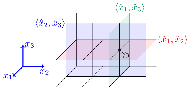
Figure 7: All the three smooth 2-dim subcomplex leaves attached to $\gamma_{0}$ in 3-dim cubical lattice/complex under PBC, where each leaf $l$ is assigned with a $B$ term of the $[0,1,2,3]$ model, denoted by $B_{\gamma_{0},l}$.

Although Fig. 7 appears similar to Fig. 1, the underlying manifold in Fig. 7 is now a curved space ($T^{3}$). Therefore, interpreting leaves as truncated vector/Euclidean spaces is no longer applicable. A proper description for the desired leaves is smooth subcomplex leaves, which do not exhibit any angular discontinuities and contain full closed $n$-cubes within them. We continue to use the symbol $\langle\hat{x}_{i_{1}},\hat{x}_{i_{2}},\dots,\hat{x}_{i_{d_{l}}}\rangle$ to represent subcomplex leaves, but they are no longer considered truncated vector/Euclidean spaces.

The foliation and cellulation structure introduced in this subsection were utilized to construct the X-cube model on general 3-dimensional manifolds [21] and the foliated fracton phase classification theory [143]. Later, it was observed that the long-range entanglement pattern of TD models extends beyond the description of foliated fracton orders, due to the nested foliation structure in TD models [22]. For a more detailed discussion, see Sec. II.4.

Appendix B Algebraic Demonstration for the SQC in Sec. III.5

In this appendix, we demonstrate the SQC in Sec. III.5 indeed prepares a ground state of $[d_{n},d,d_{l},D]$ model, when the model is a stabilizer code.

Although there are non-trivial TD models when $d=D$, e.g. $[0,1,1,1]$ model, the 1-dim transverse-field Ising model, TD models are trivial when they are stabilizer codes and simultaneously satisfy $d=D$, since that would directly lead to a unique ground state $|++\cdots+\rangle$, without LRE. The SQC for preparing $|++\cdots+\rangle$ is identity $\mathbb{I}$: all spins are elected as representative spins of $\gamma_{D}$ they associate with, the 0-step SQC $\mathbb{I}$ is unified in Eq. (103). In fact, there is no stabilizer code TD model with $d=D$, since when $d=D$, $d=d_{l}=D$, $B_{\gamma_{D}}=Z_{\gamma_{D}}$, and $Z_{\gamma_{D}}$ is not commutable with any product of pauli $X$ (except identity).

In the rest of Appendix B, we focus on the case where $d<D$.

Break the mission to 5 tasks:

Task 1: Demonstrate that the CNOT gates in the same layer of any specific part of any specific step are mutually commutable.

Task 2: Demonstrate that different parts in the same step are mutually commutable.

Task 3: Demonstrate that $\forall k\geq 1$, the CNOT gates in steps $1,\cdots,k$ do not overlap with the control qubits in step $k+1$ (i.e. the spins in $|X=1\rangle$ state used as control qubits in step $k+1$), so that steps $1,\cdots,k$ and

$$\prod_{S_{k}}\prod_{x_{i}\in\mathbb{Z}_{L_{i}-1},\,i\in S_{k}^{c}}\text{Had}_{[-\frac{1}{2},\cdots,-\frac{1}{2},x_{i}+\frac{1}{2},x_{j}|i\in\max_{d-k}(S_{k}^{c}),j\in\min_{D^{*}}(S_{k}^{c})]}$$

are commutable.

Task 4: Deduce each step algebraically.

Task 5: Demonstrate that $A$ term redundancies generate the rest of EWSCs that are not explicitly created by SQC.

B.1 Task 1

Reminder of task 1: Demonstrate that the CNOT gates in the same layer of any specific part of any specific step are mutually commutable.

Start with Eq. (103). For the convenience of derivation, we expose the information out in the derivation. In this task, we rewrite Eq. (103) as the following form: the layer $\alpha$ of part $S_{k}$ of step $k+1$ is

$$\prod_{\begin{subarray}{c}x_{i}\in\mathbb{Z}_{L_{i}-1},\,i\in S_{k}^{c}\\ \sum_{i\in\min_{D^{*}}(S_{k}^{c})}x_{i}=n(\alpha)\end{subarray}}\ \prod_{\begin{subarray}{c}\gamma_{d}\subset[-\frac{1}{2},\cdots,-\frac{1}{2},x_{i}+\frac{1}{2}|i\in S_{k}^{c}]\\ \gamma_{d}\neq[-\frac{1}{2},\cdots,-\frac{1}{2},x_{i}+\frac{1}{2},x_{j}|i\in\text{max}_{d-k}(S_{k}^{c}),j\in\min_{D^{*}}(S_{k}^{c})]\end{subarray}}$$

$$\text{CNOT}_{[-\frac{1}{2},\cdots,-\frac{1}{2},x_{i}+\frac{1}{2},x_{j}|i\in\text{max}_{d-k}(S_{k}^{c}),j\in\min_{D^{*}}(S_{k}^{c})],\gamma_{d}}\,.$$ (136)

Case 1: For two CNOT gates in Eq. (136) with the same control qubits, they are obviously commutable.
Case 2: For two CNOT gates in Eq. (136) with the control qubits having only $x_{i}$-coordinates being different, where $i\in\text{max}_{d-k}(S_{k}^{c})$, e.g.

$$\text{CNOT}_{[-\frac{1}{2},\cdots,-\frac{1}{2},x_{i}+\frac{1}{2},x_{j}|i\in\text{max}_{d-k}(S_{k}^{c}),j\in\text{min}_{D^{*}}(S_{k}^{c})],\gamma_{d}}$$ (137)

and

$$\text{CNOT}_{[-\frac{1}{2},\cdots,-\frac{1}{2},x^{\prime}_{i}+\frac{1}{2},x_{j}|i\in\text{max}_{d-k}(S_{k}^{c}),j\in\text{min}_{D^{*}}(S_{k}^{c})],\gamma^{\prime}_{d}}\,,$$ (138)

where $\Big{(}x_{i}\Big{|}i\in\text{max}_{d-k}(S_{k}^{c})\Big{)}\neq\Big{(}x^{\prime}_{i}\Big{|}i\in\text{max}_{d-k}(S_{k}^{c})\Big{)}$. Without losing generality, assume $x_{i_{0}}\neq x^{\prime}_{i_{0}}$. The target qubit of one CNOT gate (e.g. $\gamma^{\prime}_{d}$) does not overlap with the control qubit of another CNOT gate (i.e. the control qubit of Eq. (137)), since their $x_{i_{0}}$-coordinates are different:

$$x_{i_{0}}(\gamma^{\prime}_{d})\in\left[x^{\prime}_{i_{0}}+\frac{1}{2}-\frac{1}{2},x^{\prime}_{i_{0}}+\frac{1}{2}+\frac{1}{2}\right]\,,$$ (139)

but $x_{i_{0}}\neq x^{\prime}_{i_{0}}\Rightarrow x_{i_{0}}\notin(x^{\prime}_{i_{0}}-1,x^{\prime}_{i_{0}}+1)\Rightarrow$

$$x_{i_{0}}+\frac{1}{2}\notin\left(x^{\prime}_{i_{0}}+\frac{1}{2}-1,x^{\prime}_{i_{0}}+\frac{1}{2}+1\right)\supset\left[x^{\prime}_{i_{0}}+\frac{1}{2}-\frac{1}{2},x^{\prime}_{i_{0}}+\frac{1}{2}+\frac{1}{2}\right]\,.$$ (140)

$x_{i_{0}}+\frac{1}{2}$ is the $x_{i_{0}}$-coordinate of the control qubit of Eq. (137). For the two arbitrarily chosen CNOT gates Eqs. (137,138), the targer qubit of one CNOT gate does not overlap with the control qubit of another CNOT gate, the two CNOT gates are commutable.
Case 3: For two CNOT gates in Eq. (136) with the control qubits having only $x_{j}$-coordinates being different, where $j\in\text{min}_{D^{*}}(S_{k}^{c})$, e.g.

$$\text{CNOT}_{[-\frac{1}{2},\cdots,-\frac{1}{2},x_{i}+\frac{1}{2},x_{j}|i\in\text{max}_{d-k}(S_{k}^{c}),j\in\text{min}_{D^{*}}(S_{k}^{c})],\gamma_{d}}$$ (141)

and

$$\text{CNOT}_{[-\frac{1}{2},\cdots,-\frac{1}{2},x_{i}+\frac{1}{2},x^{\prime}_{j}|i\in\text{max}_{d-k}(S_{k}^{c}),j\in\text{min}_{D^{*}}(S_{k}^{c})],\gamma^{\prime}_{d}}$$ (142)

where $\Big{(}x_{j}\Big{|}j\in\text{min}_{D^{*}}(S_{k}^{c})\Big{)}\neq\Big{(}x^{\prime}_{j}\Big{|}j\in\text{min}_{D^{*}}(S_{k}^{c})\Big{)}$, the target qubit of one CNOT gate (e.g. $\gamma^{\prime}_{d}$) do not overlap with the control qubit of another CNOT gate (i.e. the control qubit of Eq. (141)), since the coordinate sum

$$\sum_{j\in\text{min}_{D^{*}}(S_{k}^{c})}x_{j}(\gamma^{\prime}_{d})\ \ \ \ \ \,>\sum_{j\in\text{min}_{D^{*}}(S_{k}^{c})}x^{\prime}_{j}\ \ \ \ \ \,=\ \ \ \ \ \,n(\alpha)\ \ \ \ \ \,=\sum_{j\in\text{min}_{D^{*}}(S_{k}^{c})}x_{j}$$ (143)

The inequality in Eq. (143) is true since $\gamma^{\prime}_{d}$ and

$$\left.\left[-\frac{1}{2},\cdots,-\frac{1}{2},x_{i}+\frac{1}{2},x^{\prime}_{j}\right|i\in\text{max}_{d-k}(S_{k}^{c}),j\in\text{min}_{D^{*}}(S_{k}^{c})\right]$$ (144)

are the cubes of same dimension in

$$\left.\left[-\frac{1}{2},\cdots,-\frac{1}{2},x_{i}+\frac{1}{2}\right|i\in S_{k}^{c}\right]\ :=\ \gamma_{D,0}\,,$$ (145)

and Eq. (144) is the unique $\gamma_{d}$ in $\gamma_{D,0}$ with the smallest coordinate sum $\sum_{j\in\text{min}_{D^{*}}(S_{k}^{c})}x_{j}$: it is unique since being a $d$-cube requires $d$ coordinates being half-integer, or equivalently, $D-d=D^{*}$ coordinates have to be integer, the $\gamma_{d}$ Eq. (144) has the $D^{*}$ coordinates in $\text{min}_{D^{*}}(S_{k}^{c})$ reaching the minimal integers available, given Eq. (144)$\in\gamma_{D,0}$, so Eq. (144) uniquely reaches the minimum of $\sum_{j\in\text{min}_{D^{*}}(S_{k}^{c})}x_{j}$. Note that the case where $d<D\Leftrightarrow D^{*}>0$ is considered here, which means $\text{min}_{D^{*}}(S_{k}^{c})\neq\emptyset$, this condition is needed here. The case where $d=D$ was discussed at the begining of appendix B. For the two arbitrarily chosen CNOT gates Eqs. (141,142), the target qubit of one CNOT gate does not overlap with the control qubit of another CNOT gate, the two CNOT gates are commutable.
Case 4: For two CNOT gates in Eq. (136) with the control qubits having both $x_{i}$-coordinates and $x_{j}$-coordinates being different, where $i\in\text{max}_{d-k}(S_{k}^{c})$, $j\in\text{min}_{D^{*}}(S_{k}^{c})$, from either the deduction for $x_{i}$ different case (case 2) or the deduction for $x_{j}$ different case (case 3) above, one could see that they are commutable.

B.2 Task 2

Reminder of task 2: Demonstrate that different parts in the same step are mutually commutable.

In task 2, we write each part as a whole, rather than write each layer of a part separately.
Consider part $S_{k}$ and part $S^{\prime}_{k}$ of step $k+1$, i.e.

$$\prod_{n=0}^{\sum_{i\in\text{min}_{D^{*}}(S_{k}^{c})}(L_{i}-2)}\prod_{\begin{subarray}{c}x_{i}\in\mathbb{Z}_{L_{i}-1},\,i\in S_{k}^{c}\\ \sum_{i\in\text{min}_{D^{*}}(S_{k}^{c})}x_{i}=n\end{subarray}}\text{GCNOT}_{[-\frac{1}{2},\cdots,-\frac{1}{2},x_{i}+\frac{1}{2},x_{j}|i\in\text{max}_{d-k}(S_{k}^{c}),j\in\text{min}_{D^{*}}(S_{k}^{c})]}^{\delta_{d}[-\frac{1}{2},\cdots,-\frac{1}{2},x_{i}+\frac{1}{2}|i\in S_{k}^{c}]}$$ (146)

and

$$\prod_{n=0}^{\sum_{i\in\text{min}_{D^{*}}(S^{\prime c}_{k})}(L_{i}-2)}\prod_{\begin{subarray}{c}x_{i}\in\mathbb{Z}_{L_{i}-1},\,i\in S^{\prime c}_{k}\\ \sum_{i\in\text{min}_{D^{*}}(S^{\prime c}_{k})}x_{i}=n\end{subarray}}\text{GCNOT}_{[-\frac{1}{2},\cdots,-\frac{1}{2},x_{i}+\frac{1}{2},x_{j}|i\in\text{max}_{d-k}(S^{\prime c}_{k}),j\in\text{min}_{D^{*}}(S^{\prime c}_{k})]}^{\delta_{d}[-\frac{1}{2},\cdots,-\frac{1}{2},x_{i}+\frac{1}{2}|i\in S^{\prime c}_{k}]}\,,$$ (147)

where $S_{k}\neq S^{\prime}_{k}$. Since $k,S_{k},S^{\prime}_{k}$ are arbitrary, it is enough to demonstrate that no control qubit in part $S_{k}$ is target qubit in part $S^{\prime}_{k}$ (again to use that a set of CNOT gates with no qubit being control qubit and target qubit at the same time are mutually commutable).
The control qubits in part $S_{k}$ are on one of the following $\gamma_{d}$:

$$\left.\left[-\frac{1}{2},\cdots,-\frac{1}{2},x_{i}+\frac{1}{2},x_{j}\right|i\in\text{max}_{d-k}(S_{k}^{c}),j\in\text{min}_{D^{*}}(S_{k}^{c})\right]\ ,\quad x_{i}\in\mathbb{Z}_{L_{i}-1},\ i\in S_{k}^{c}$$ (148)

The CNOT gates in part $S^{\prime}_{k}$ are inside one of the following (closed) $\gamma_{D}$:

$$\left.\left[-\frac{1}{2},\cdots,-\frac{1}{2},x_{i}+\frac{1}{2}\right|i\in S^{\prime c}_{k}\right]\ ,\quad x_{i}\in\mathbb{Z}_{L_{i}-1},\ i\in S^{\prime c}_{k}$$ (149)

All and only $x_{p}$-coordinates (where $p\in S_{k}$) of $\gamma_{d}$ in Eq. (148) are $-\frac{1}{2}$. All and only $x_{q}$-coordinates (where $q\in S^{\prime}_{k}$) of $\gamma_{D}$ in Eq. (149) are $-\frac{1}{2}$. Since $S_{k}\neq S^{\prime}_{k}$, there exists at least one direction $p_{0}\in S_{k}$, s.t. $p_{0}\notin S^{\prime}_{k}$, thus the $x_{p_{0}}$-coordinate of $\gamma_{d}$ in Eq. (148) is $-\frac{1}{2}$, and the $x_{p_{0}}$-coordinate of $\gamma_{D}$ in Eq. (149) is not $-\frac{1}{2}$. The $x_{p_{0}}$-coordinate of any $\gamma_{D}$ in Eq. (149) belongs to $\left[\frac{1}{2},L_{x_{p_{0}}}-\frac{3}{2}\right]$, so the $x_{p_{0}}$-coordinate of any $\gamma_{d}$ in $\delta_{d}\gamma_{D}$ of $\gamma_{D}$ in Eq. (149) belongs to $[0,L_{x_{p_{0}}}-1]$, which does not contain $-\frac{1}{2}=L_{x_{p_{0}}}-\frac{1}{2}$. Therefore, $\gamma_{d}$ in Eq. (148) do not overlap with $\gamma_{d}$ in $\delta_{d}\gamma_{D}$ of $\gamma_{D}$ in Eq. (149), nor be target qubits in part $S^{\prime}_{k}$.

For simplicity, we shortly/pictorially say “$\gamma_{d}$ inside $\gamma_{D}$” for “$\gamma_{d}$ in $\delta_{d}\gamma_{D}$ of $\gamma_{D}$” hereafter.

B.3 Task 3

Reminder of task 3: Demonstrate that $\forall k\geq 1$, the CNOT gates in steps $1,\cdots,k$ do not overlap with the control qubits in step $k+1$ (i.e. the spins in $|X=1\rangle$ state used as control qubits in step $k+1$), so that steps $1,\cdots,k$ and

$$\prod_{S_{k}}\prod_{x_{i}\in\mathbb{Z}_{L_{i}-1},\,i\in S_{k}^{c}}\text{Had}_{[-\frac{1}{2},\cdots,-\frac{1}{2},x_{i}+\frac{1}{2},x_{j}|i\in\max_{d-k}(S_{k}^{c}),j\in\min_{D^{*}}(S_{k}^{c})]}$$

are commutable.

Task 3 is equivalent to demonstrating that $\forall k\geq 1$, the CNOT gates in step $m+1\ (\forall m=0,\cdots,k-1)$ do not overlap with control qubits in step $k+1$.
In task 3, we write each step as a whole, rather than writing each part separately.
Step $k+1$ is

$$\begin{split}\prod_{S_{k}}\prod_{n=0}^{\sum_{i\in\text{min}_{D^{*}}(S_{k}^{c})}(L_{i}-2)}\prod_{\begin{subarray}{c}x_{i}\in\mathbb{Z}_{L_{i}-1},\,i\in S_{k}^{c}\\ \sum_{i\in\text{min}_{D^{*}}(S_{k}^{c})}x_{i}=n\end{subarray}}\text{GCNOT}_{[-\frac{1}{2},\cdots,-\frac{1}{2},x_{i}+\frac{1}{2},x_{j}|i\in\text{max}_{d-k}(S_{k}^{c}),j\in\text{min}_{D^{*}}(S_{k}^{c})]}^{\delta_{d}[-\frac{1}{2},\cdots,-\frac{1}{2},x_{i}+\frac{1}{2}|i\in S_{k}^{c}]}\,.\end{split}$$ (150)

$\forall k\geq 1$, $\forall m=0,\cdots,k-1$, the CNOT gates in step $m+1$ are inside one of the following $\gamma_{D}$:

$$\left.\left[-\frac{1}{2},\cdots,-\frac{1}{2},x_{i}+\frac{1}{2}\right|i\in S_{m}^{c}\right]\ ,\quad x_{i}\in\mathbb{Z}_{L_{i}-1},\ i\in S_{m}^{c}$$ (151)

with some $S_{m}\subset\{1:D\}$, $|S_{m}|=m$. The control qubits in step $k+1$ are on one of the following $\gamma_{d}$:

$$\left.\left[-\frac{1}{2},\cdots,-\frac{1}{2},x_{i}+\frac{1}{2},x_{j}\right|i\in\text{max}_{d-k}(S_{k}^{c}),j\in\text{min}_{D^{*}}(S_{k}^{c})\right]\ ,\quad x_{i}\in\mathbb{Z}_{L_{i}-1},\ i\in S_{k}^{c}$$ (152)

with some $S_{k}\subset\{1:D\}$, $|S_{k}|=k$. There are $m$ coordinates being $-\frac{1}{2}$ for $\gamma_{D}$ in Eq. (151), and $k$ coordinates being $-\frac{1}{2}$ for $\gamma_{d}$ in Eq. (152). Since $k>m$, no matter what $S_{k}$ is, there always exists at least one direction $x_{i_{0}}$, where the $x_{i_{0}}$-coordinate of $\gamma_{d}$ in Eq. (152) is $-\frac{1}{2}$, and the $x_{i_{0}}$-coordinate of $\gamma_{D}$ in Eq. (151) is not $-\frac{1}{2}$. The $\gamma_{D}$ in Eq. (151) with largest $x_{i_{0}}$-coordinate have $x_{i_{0}}=L_{x_{i_{0}}}-\frac{3}{2}$, so the $\gamma_{d}$ inside at least one $\gamma_{D}$ in Eq. (151) have at most $x_{i_{0}}=L_{x_{i_{0}}}-1<L_{x_{i_{0}}}-\frac{1}{2}\big{(}=-\frac{1}{2}\ \text{mod}\ L_{x_{i_{0}}}\big{)}$. And the $\gamma_{D}$ in Eq. (151) with smallest $x_{i_{0}}$-coordinate have $x_{i_{0}}=\frac{1}{2}$, so the $\gamma_{d}$ inside at least one (closed) $\gamma_{D}$ in Eq. (151) have at least $x_{i_{0}}=0>-\frac{1}{2}$. The $\gamma_{d}$ in Eq. (152) all have $x_{i_{0}}=-\frac{1}{2}$, so there is no overlap between Eq. (151) and Eq. (152). Proved.

B.4 Task 4

Reminder of task 4: Deduce each step algebraically.

The state after step 0 is

$$|\Phi_{0}\rangle:=\prod_{k=0}^{d}\prod_{S_{k}}\prod_{x_{i}\in\mathbb{Z}_{L_{i}-1},\,i\in S_{k}^{c}}\text{Had}_{[-\frac{1}{2},\cdots,-\frac{1}{2},x_{i}+\frac{1}{2},x_{j}|i\in\text{max}_{d-k}(S_{k}^{c}),j\in\text{min}_{D^{*}}(S_{k}^{c})]}\Big{|}00\cdots 0\Big{\rangle}\,.$$ (153)

Use mathematical induction to prove task 4:
Assume $\forall k^{\prime}=0,1,\cdots,d+1$, the state after step $k^{\prime}$ is

$$|\Phi_{k^{\prime}}\rangle:=$$

$$\Bigg{(}\prod_{k=k^{\prime}}^{d}\prod_{S_{k}}\prod_{x_{i}\in\mathbb{Z}_{L_{i}-1},\,i\in S_{k}^{c}}\text{Had}_{[-\frac{1}{2},\cdots,-\frac{1}{2},x_{i}+\frac{1}{2},x_{j}|i\in\text{max}_{d-k}(S_{k}^{c}),j\in\text{min}_{D^{*}}(S_{k}^{c})]}\Bigg{)}$$

$$\Bigg{(}\prod_{k=0}^{k^{\prime}-1}\prod_{S_{k}}\prod_{x_{i}\in\mathbb{Z}_{L_{i}-1},\,i\in S_{k}^{c}}\frac{1}{\sqrt{2}}\Big{(}1+A_{[-\frac{1}{2},\cdots,-\frac{1}{2},x_{i}+\frac{1}{2}|i\in S_{k}^{c}]}\Big{)}\Bigg{)}\Big{|}00\cdots 0\Big{\rangle}$$ (154)

The state after step $k^{\prime}=0$ is indeed Eq. (154). Once we prove $\forall k^{\prime}=0,1,\cdots,d$, the result state of applying step $k^{\prime}+1$ on $|\Phi_{k^{\prime}}\rangle$ is

$$|\Phi_{k^{\prime}+1}\rangle:=$$

$$\Bigg{(}\prod_{k=k^{\prime}+1}^{d}\,\prod_{S_{k}}\prod_{x_{i}\in\mathbb{Z}_{L_{i}-1},\,i\in S_{k}^{c}}\text{Had}_{[-\frac{1}{2},\cdots,-\frac{1}{2},x_{i}+\frac{1}{2},x_{j}|i\in\text{max}_{d-k}(S_{k}^{c}),j\in\text{min}_{D^{*}}(S_{k}^{c})]}\Bigg{)}$$

$$\Bigg{(}\prod_{k=0}^{k^{\prime}}\prod_{S_{k}}\prod_{x_{i}\in\mathbb{Z}_{L_{i}-1},\,i\in S_{k}^{c}}\frac{1}{\sqrt{2}}\Big{(}1+A_{[-\frac{1}{2},\cdots,-\frac{1}{2},x_{i}+\frac{1}{2}|i\in S_{k}^{c}]}\Big{)}\Bigg{)}\Big{|}00\cdots 0\Big{\rangle}$$ (155)

The assumption Eq. (154) is nearly proved (the last step is just combining with the fact that the state after step 0 is $|\Psi_{0}\rangle$).
Step $k^{\prime}+1$ is

$$\prod_{S_{k^{\prime}}}\prod_{n=0}^{\sum_{i\in\text{min}_{D^{*}}(S^{c}_{k^{\prime}})}(L_{i}-2)}\prod_{\begin{subarray}{c}x_{i}\in\mathbb{Z}_{L_{i}-1},\,i\in S^{c}_{k^{\prime}}\\ \sum_{i\in\text{min}_{D^{*}}(S^{c}_{k^{\prime}})}x_{i}=n\end{subarray}}\text{GCNOT}_{[-\frac{1}{2},\cdots,-\frac{1}{2},x_{i}+\frac{1}{2},x_{j}|i\in\text{max}_{d-k^{\prime}}(S^{c}_{k^{\prime}}),j\in\text{min}_{D^{*}}(S^{c}_{k^{\prime}})]}^{\delta_{d}[-\frac{1}{2},\cdots,-\frac{1}{2},x_{i}+\frac{1}{2}|i\in S^{c}_{k^{\prime}}]}$$ (156)

Apply step $k^{\prime}+1$ on Eq. (154), the result state is

$$\Bigg{(}\prod_{S_{k^{\prime}}}\prod_{n=0}^{\sum_{i\in\text{min}_{D^{*}}(S^{c}_{k^{\prime}})}(L_{i}-2)}\prod_{\begin{subarray}{c}x_{i}\in\mathbb{Z}_{L_{i}-1},\,i\in S^{c}_{k^{\prime}}\\ \sum_{i\in\text{min}_{D^{*}}(S^{c}_{k^{\prime}})}x_{i}=n\end{subarray}}\text{GCNOT}_{[-\frac{1}{2},\cdots,-\frac{1}{2},x_{i}+\frac{1}{2},x_{j}|i\in\text{max}_{d-k^{\prime}}(S^{c}_{k^{\prime}}),j\in\text{min}_{D^{*}}(S^{c}_{k^{\prime}})]}^{\delta_{d}[-\frac{1}{2},\cdots,-\frac{1}{2},x_{i}+\frac{1}{2}|i\in S^{c}_{k^{\prime}}]}\Bigg{)}$$

$$\Bigg{(}\prod_{k=k^{\prime}}^{d}\prod_{S_{k}}\prod_{x_{i}\in\mathbb{Z}_{L_{i}-1},\,i\in S_{k}^{c}}\text{Had}_{[-\frac{1}{2},\cdots,-\frac{1}{2},x_{i}+\frac{1}{2},x_{j}|i\in\text{max}_{d-k}(S_{k}^{c}),j\in\text{min}_{D^{*}}(S_{k}^{c})]}\Bigg{)}$$

$$\Bigg{(}\prod_{k=0}^{k^{\prime}-1}\prod_{S_{k}}\prod_{x_{i}\in\mathbb{Z}_{L_{i}-1},\,i\in S_{k}^{c}}\frac{1}{\sqrt{2}}\Big{(}1+A_{[-\frac{1}{2},\cdots,-\frac{1}{2},x_{i}+\frac{1}{2}|i\in S_{k}^{c}]}\Big{)}\Bigg{)}\Big{|}00\cdots 0\Big{\rangle}$$ (157)

For the $\gamma_{d}$ associated with Had in Eq. (157), there are at least $k^{\prime}$ coordinates being $-\frac{1}{2}$.
For the $\gamma_{D}$ associated with $A$ term in Eq. (157), there are at most $k^{\prime}-1$ coordinates being $-\frac{1}{2}$.
Therefore $\forall\gamma_{d}$ associated with Had in Eq. (157), there exists at least one coordinate $x_{i_{0}}$, s.t. the $x_{i_{0}}$-coordinate of $\gamma_{d}$ associated with Had in Eq. (157) is $-\frac{1}{2}$, and the $x_{i_{0}}$-coordinate of $\gamma_{D}$ associated with $A$ term in Eq. (157) is not $-\frac{1}{2}$. The $x_{i_{0}}$-coordinate of $\gamma_{D}$ associated with $A$ term in Eq. (157) belongs to $\left[\frac{1}{2},L_{x_{i_{0}}}-\frac{3}{2}\right]$, so the $x_{i_{0}}$-coordinate of $\gamma_{d}$ inside (closed) $\gamma_{D}$ associated with $A$ term in Eq. (157) belongs to $\left[0,L_{x_{i_{0}}}-1\right]$, which does not contain $-\frac{1}{2}$, the $x_{i_{0}}$-coordinate of $\gamma_{d}$ associated with Had in Eq. (157). Therefore, there is no overlap between $\gamma_{d}$ associated with Had in Eq. (157) and $\gamma_{d}$ in $\gamma_{D}$ associated with $A$ term in Eq. (157), all Had and $A$ terms in Eq. (157) are commutable.
So we can commute part of them and write

$$\text{(\ref*{dddd_SQC_148})}=$$

$$\Bigg{(}\prod_{S_{k^{\prime}}}\prod_{n=0}^{\sum_{i\in\text{min}_{D^{*}}(S^{c}_{k^{\prime}})}(L_{i}-2)}\prod_{\begin{subarray}{c}x_{i}\in\mathbb{Z}_{L_{i}-1},\,i\in S^{c}_{k^{\prime}}\\ \sum_{i\in\text{min}_{D^{*}}(S^{c}_{k^{\prime}})}x_{i}=n\end{subarray}}\text{GCNOT}_{[-\frac{1}{2},\cdots,-\frac{1}{2},x_{i}+\frac{1}{2},x_{j}|i\in\text{max}_{d-k^{\prime}}(S^{c}_{k^{\prime}}),j\in\text{min}_{D^{*}}(S^{c}_{k^{\prime}})]}^{\delta_{d}[-\frac{1}{2},\cdots,-\frac{1}{2},x_{i}+\frac{1}{2}|i\in S^{c}_{k^{\prime}}]}\Bigg{)}$$

$$\Bigg{(}\prod_{k=k^{\prime}+1}^{d}\prod_{S_{k}}\prod_{x_{i}\in\mathbb{Z}_{L_{i}-1},\,i\in S_{k}^{c}}\text{Had}_{[-\frac{1}{2},\cdots,-\frac{1}{2},x_{i}+\frac{1}{2},x_{j}|i\in\text{max}_{d-k}(S_{k}^{c}),j\in\text{min}_{D^{*}}(S_{k}^{c})]}\Bigg{)}$$

$$\Bigg{(}\prod_{k=0}^{k^{\prime}-1}\prod_{S_{k}}\prod_{x_{i}\in\mathbb{Z}_{L_{i}-1},\,i\in S_{k}^{c}}\frac{1}{\sqrt{2}}\Big{(}1+A_{[-\frac{1}{2},\cdots,-\frac{1}{2},x_{i}+\frac{1}{2}|i\in S_{k}^{c}]}\Big{)}\Bigg{)}$$

$$\Bigg{(}\prod_{S_{k^{\prime}}}\prod_{x_{i}\in\mathbb{Z}_{L_{i}-1},\,i\in S^{c}_{k^{\prime}}}\text{Had}_{[-\frac{1}{2},\cdots,-\frac{1}{2},x_{i}+\frac{1}{2},x_{j}|i\in\text{max}_{d-k^{\prime}}(S^{c}_{k^{\prime}}),j\in\text{min}_{D^{*}}(S^{c}_{k^{\prime}})]}\Bigg{)}\Big{|}00\cdots 0\Big{\rangle}$$ (157.1)

Use $\text{Had}|0\rangle=\frac{1}{\sqrt{2}}(Z+X)|0\rangle=\frac{1}{\sqrt{2}}(1+X)|0\rangle$,

$$\text{(\ref*{dddd_SQC_148}.1)}=$$

$$\Bigg{(}\prod_{S_{k^{\prime}}}\prod_{n=0}^{\sum_{i\in\text{min}_{D^{*}}(S^{c}_{k^{\prime}})}(L_{i}-2)}\prod_{\begin{subarray}{c}x_{i}\in\mathbb{Z}_{L_{i}-1},\,i\in S^{c}_{k^{\prime}}\\ \sum_{i\in\text{min}_{D^{*}}(S^{c}_{k^{\prime}})}x_{i}=n\end{subarray}}\text{GCNOT}_{[-\frac{1}{2},\cdots,-\frac{1}{2},x_{i}+\frac{1}{2},x_{j}|i\in\text{max}_{d-k^{\prime}}(S^{c}_{k^{\prime}}),j\in\text{min}_{D^{*}}(S^{c}_{k^{\prime}})]}^{\delta_{d}[-\frac{1}{2},\cdots,-\frac{1}{2},x_{i}+\frac{1}{2}|i\in S^{c}_{k^{\prime}}]}\Bigg{)}$$

$$\Bigg{(}\prod_{k=k^{\prime}+1}^{d}\prod_{S_{k}}\prod_{x_{i}\in\mathbb{Z}_{L_{i}-1},\,i\in S_{k}^{c}}\text{Had}_{[-\frac{1}{2},\cdots,-\frac{1}{2},x_{i}+\frac{1}{2},x_{j}|i\in\text{max}_{d-k}(S_{k}^{c}),j\in\text{min}_{D^{*}}(S_{k}^{c})]}\Bigg{)}$$

$$\Bigg{(}\prod_{k=0}^{k^{\prime}-1}\prod_{S_{k}}\prod_{x_{i}\in\mathbb{Z}_{L_{i}-1},\,i\in S_{k}^{c}}\frac{1}{\sqrt{2}}\Big{(}1+A_{[-\frac{1}{2},\cdots,-\frac{1}{2},x_{i}+\frac{1}{2}|i\in S_{k}^{c}]}\Big{)}\Bigg{)}$$

$$\Bigg{(}\prod_{S_{k^{\prime}}}\prod_{x_{i}\in\mathbb{Z}_{L_{i}-1},\,i\in S^{c}_{k^{\prime}}}\frac{1}{\sqrt{2}}\Big{(}1+X_{[-\frac{1}{2},\cdots,-\frac{1}{2},x_{i}+\frac{1}{2},x_{j}|i\in\text{max}_{d-k^{\prime}}(S^{c}_{k^{\prime}}),j\in\text{min}_{D^{*}}(S^{c}_{k^{\prime}})]}\Big{)}\Bigg{)}\Big{|}00\cdots 0\Big{\rangle}$$ (157.2)

Each GCNOT in Eq. (157.2) is associated with a $\gamma_{D}$.
Now we want to prove the GCNOT and Had in Eq. (157.2) are commutable.
If $k^{\prime}=d$, $\prod_{k=k^{\prime}+1}^{d}\cdots=1$, $\nexists$ Had in Eq. (157.2), GCNOT and 1 are commutable.
If $k^{\prime}=0,1,\cdots,d-1$:

• for the $\gamma_{D}$ associated with GCNOT in Eq. (157.2), there are $k^{\prime}$ coordinates being $-\frac{1}{2}$;

• for the $\gamma_{d}$ associated with Had in Eq. (157.2), there are at least $k^{\prime}+1$ coordinates being $-\frac{1}{2}$;

• so for any $\gamma_{d}$ associated with Had in Eq. (157.2), there always exists at least one coordinate $x_{i_{0}}$, s.t. the $x_{i_{0}}$-coordinate of $\gamma_{d}$ associated with Had in Eq. (157.2) is $-\frac{1}{2}$, and the $x_{i_{0}}$-coordinate of $\gamma_{D}$ associated with GCNOT in Eq. (157.2) is not $-\frac{1}{2}$. The $x_{i_{0}}$-coordinate of $\gamma_{D}$ associated with GCNOT in Eq. (157.2) belongs to $\left[\frac{1}{2},L_{x_{i_{0}}}-\frac{3}{2}\right]$, so the $x_{i_{0}}$-coordinate of $\gamma_{d}$ inside $\gamma_{D}$ associated with GCNOT in Eq. (157.2) belongs to $[0,L_{x_{i_{0}}}-1]$, which does not contain $-\frac{1}{2}$, the $x_{i_{0}}$-coordinate of $\gamma_{d}$ associated with Had in Eq. (157.2). Therefore, there is no overlap between GCNOT and Had in Eq. (157.2), they are commutable.

So,

$$\text{(\ref*{dddd_SQC_148}.2)}=$$

$$\Bigg{(}\prod_{k=k^{\prime}+1}^{d}\prod_{S_{k}}\prod_{x_{i}\in\mathbb{Z}_{L_{i}-1},\,i\in S_{k}^{c}}\text{Had}_{[-\frac{1}{2},\cdots,-\frac{1}{2},x_{i}+\frac{1}{2},x_{j}|i\in\text{max}_{d-k}(S_{k}^{c}),j\in\text{min}_{D^{*}}(S_{k}^{c})]}\Bigg{)}$$

$$\Bigg{(}\prod_{S_{k^{\prime}}}\prod_{n=0}^{\sum_{i\in\text{min}_{D^{*}}(S^{c}_{k^{\prime}})}(L_{i}-2)}\prod_{\begin{subarray}{c}x_{i}\in\mathbb{Z}_{L_{i}-1},\,i\in S^{c}_{k^{\prime}}\\ \sum_{i\in\text{min}_{D^{*}}(S^{c}_{k^{\prime}})}x_{i}=n\end{subarray}}\text{GCNOT}_{[-\frac{1}{2},\cdots,-\frac{1}{2},x_{i}+\frac{1}{2},x_{j}|i\in\text{max}_{d-k^{\prime}}(S^{c}_{k^{\prime}}),j\in\text{min}_{D^{*}}(S^{c}_{k^{\prime}})]}^{\delta_{d}[-\frac{1}{2},\cdots,-\frac{1}{2},x_{i}+\frac{1}{2}|i\in S^{c}_{k^{\prime}}]}\Bigg{)}$$

$$\Bigg{(}\prod_{k=0}^{k^{\prime}-1}\prod_{S_{k}}\prod_{x_{i}\in\mathbb{Z}_{L_{i}-1},\,i\in S_{k}^{c}}\frac{1}{\sqrt{2}}\Big{(}1+A_{[-\frac{1}{2},\cdots,-\frac{1}{2},x_{i}+\frac{1}{2}|i\in S_{k}^{c}]}\Big{)}\Bigg{)}$$

$$\Bigg{(}\prod_{S_{k^{\prime}}}\prod_{x_{i}\in\mathbb{Z}_{L_{i}-1},\,i\in S^{c}_{k^{\prime}}}\frac{1}{\sqrt{2}}\Big{(}1+X_{[-\frac{1}{2},\cdots,-\frac{1}{2},x_{i}+\frac{1}{2},x_{j}|i\in\text{max}_{d-k^{\prime}}(S^{c}_{k^{\prime}}),j\in\text{min}_{D^{*}}(S^{c}_{k^{\prime}})]}\Big{)}\Bigg{)}\Big{|}00\cdots 0\Big{\rangle}$$ (157.3)

Now we are going to demonstrate that the GCNOT and $A$ terms in Eq. (157.3) are commutable. $A$ terms are products of Pauli $X$ operators. GCNOT are products of CNOT. As long as a Pauli $X$ operator do not overlap with the control qubit of CNOT gate, they are commutable, i.e.

$$\big{[}\text{CNOT}_{12},X_{2}\big{]}=\big{[}\text{CNOT}_{12},X_{3}\big{]}=0$$ (158)

Note that Had does not have this property.
For the $\gamma_{d}$ associated with the control qubit of GCNOT in Eq. (157.3), there are $k^{\prime}$ coordinates being $-\frac{1}{2}$.
For the $\gamma_{D}$ associated with $A$ terms in Eq. (157.3), there are at most $k^{\prime}-1$ coordinates being $-\frac{1}{2}$.
So for any $\gamma_{d}$ associated with the control qubit of GCNOT in Eq. (157.3), there always exists at least one coordinate $x_{i_{0}}$, s.t. the $x_{i_{0}}$-coordinate of $\gamma_{d}$ associated with the control qubit of GCNOT in Eq. (157.3) is $-\frac{1}{2}$, and the $x_{i_{0}}$-coordinate of $\gamma_{D}$ associated with $A$ term in Eq. (157.3) is not $-\frac{1}{2}$. The $x_{i_{0}}$-coordinate of $\gamma_{D}$ associated with $A$ term in Eq. (157.3) belongs to $\left[\frac{1}{2},L_{x_{i_{0}}}-\frac{3}{2}\right]$, so the $x_{i_{0}}$-coordinate of $\gamma_{d}$ inside $\gamma_{D}$ associated with $A$ term in Eq. (157.3) belongs to $[0,L_{x_{i_{0}}}-1]$, which does not contain $-\frac{1}{2}$, the $x_{i_{0}}$-coordinate of $\gamma_{d}$ associated with the control qubit of GCNOT in Eq. (157.3). Therefore, there is no overlap between the $\gamma_{d}$ associated with Pauli $X$ in $A$ term in Eq. (157.3) and the $\gamma_{d}$ associated with the control qubit of GCNOT in Eq. (157.3), so according to Eq. (158), $A$ terms and GCNOT in Eq. (157.3) are commutable.
So,

$$\text{(\ref*{dddd_SQC_148}.3)}=$$

$$\Bigg{(}\prod_{k=k^{\prime}+1}^{d}\,\prod_{S_{k}}\prod_{x_{i}\in\mathbb{Z}_{L_{i}-1},\,i\in S_{k}^{c}}\text{Had}_{[-\frac{1}{2},\cdots,-\frac{1}{2},x_{i}+\frac{1}{2},x_{j}|i\in\text{max}_{d-k}(S_{k}^{c}),j\in\text{min}_{D^{*}}(S_{k}^{c})]}\Bigg{)}$$

$$\Bigg{(}\prod_{k=0}^{k^{\prime}-1}\prod_{S_{k}}\prod_{x_{i}\in\mathbb{Z}_{L_{i}-1},\,i\in S_{k}^{c}}\frac{1}{\sqrt{2}}\Big{(}1+A_{[-\frac{1}{2},\cdots,-\frac{1}{2},x_{i}+\frac{1}{2}|i\in S_{k}^{c}]}\Big{)}\Bigg{)}$$

$$\Bigg{(}\prod_{S_{k^{\prime}}}\prod_{n=0}^{\sum_{i\in\text{min}_{D^{*}}(S^{c}_{k^{\prime}})}(L_{i}-2)}\prod_{\begin{subarray}{c}x_{i}\in\mathbb{Z}_{L_{i}-1},\,i\in S^{c}_{k^{\prime}}\\ \sum_{i\in\text{min}_{D^{*}}(S^{c}_{k^{\prime}})}x_{i}=n\end{subarray}}\text{GCNOT}_{[-\frac{1}{2},\cdots,-\frac{1}{2},x_{i}+\frac{1}{2},x_{j}|i\in\text{max}_{d-k^{\prime}}(S^{c}_{k^{\prime}}),j\in\text{min}_{D^{*}}(S^{c}_{k^{\prime}})]}^{\delta_{d}[-\frac{1}{2},\cdots,-\frac{1}{2},x_{i}+\frac{1}{2}|i\in S^{c}_{k^{\prime}}]}\Bigg{)}$$

$$\Bigg{(}\prod_{S_{k^{\prime}}}\prod_{x_{i}\in\mathbb{Z}_{L_{i}-1},\,i\in S^{c}_{k^{\prime}}}\frac{1}{\sqrt{2}}\Big{(}1+X_{[-\frac{1}{2},\cdots,-\frac{1}{2},x_{i}+\frac{1}{2},x_{j}|i\in\text{max}_{d-k^{\prime}}(S^{c}_{k^{\prime}}),j\in\text{min}_{D^{*}}(S^{c}_{k^{\prime}})]}\Big{)}\Bigg{)}\Big{|}00\cdots 0\Big{\rangle}$$ (157.4)

Note that for commutable product,

$$\prod_{x_{i}\in\mathbb{Z}_{L_{i}-1},\,i\in S^{c}_{k^{\prime}}}=\prod_{n=0}^{\sum_{i\in\text{min}_{D^{*}}(S^{c}_{k^{\prime}})}(L_{i}-2)}\prod_{\begin{subarray}{c}x_{i}\in\mathbb{Z}_{L_{i}-1},\,i\in S^{c}_{k^{\prime}}\\ \sum_{i\in\text{min}_{D^{*}}(S^{c}_{k^{\prime}})}x_{i}=n\end{subarray}}$$ (159)

(Precisely speaking, the product symbol on the left above makes sense only to commutable operator.)
So Eq. (157.4) can be written as

$$\text{(\ref*{dddd_SQC_148}.4)}=$$

$$\Bigg{(}\prod_{k=k^{\prime}+1}^{d}\prod_{S_{k}}\prod_{x_{i}\in\mathbb{Z}_{L_{i}-1},\,i\in S_{k}^{c}}\text{Had}_{[-\frac{1}{2},\cdots,-\frac{1}{2},x_{i}+\frac{1}{2},x_{j}|i\in\text{max}_{d-k}(S_{k}^{c}),j\in\text{min}_{D^{*}}(S_{k}^{c})]}\Bigg{)}$$

$$\Bigg{(}\prod_{k=0}^{k^{\prime}-1}\prod_{S_{k}}\prod_{x_{i}\in\mathbb{Z}_{L_{i}-1},\,i\in S_{k}^{c}}\frac{1}{\sqrt{2}}\Big{(}1+A_{[-\frac{1}{2},\cdots,-\frac{1}{2},x_{i}+\frac{1}{2}|i\in S_{k}^{c}]}\Big{)}\Bigg{)}$$

$$\Bigg{(}\prod_{S_{k^{\prime}}}\prod_{n=0}^{\sum_{i\in\text{min}_{D^{*}}(S^{c}_{k^{\prime}})}(L_{i}-2)}\prod_{\begin{subarray}{c}x_{i}\in\mathbb{Z}_{L_{i}-1},\,i\in S^{c}_{k^{\prime}}\\ \sum_{i\in\text{min}_{D^{*}}(S^{c}_{k^{\prime}})}x_{i}=n\end{subarray}}\text{GCNOT}_{[-\frac{1}{2},\cdots,-\frac{1}{2},x_{i}+\frac{1}{2},x_{j}|i\in\text{max}_{d-k^{\prime}}(S^{c}_{k^{\prime}}),j\in\text{min}_{D^{*}}(S^{c}_{k^{\prime}})]}^{\delta_{d}[-\frac{1}{2},\cdots,-\frac{1}{2},x_{i}+\frac{1}{2}|i\in S^{c}_{k^{\prime}}]}\Bigg{)}$$

$$\Bigg{(}\prod_{S_{k^{\prime}}}\prod_{n=0}^{\sum_{i\in\text{min}_{D^{*}}(S^{c}_{k^{\prime}})}(L_{i}-2)}\prod_{\begin{subarray}{c}x_{i}\in\mathbb{Z}_{L_{i}-1},\,i\in S^{c}_{k^{\prime}}\\ \sum_{i\in\text{min}_{D^{*}}(S^{c}_{k^{\prime}})}x_{i}=n\end{subarray}}\frac{1}{\sqrt{2}}\Big{(}1+X_{[-\frac{1}{2},\cdots,-\frac{1}{2},x_{i}+\frac{1}{2},x_{j}|i\in\text{max}_{d-k^{\prime}}(S^{c}_{k^{\prime}}),j\in\text{min}_{D^{*}}(S^{c}_{k^{\prime}})]}\Big{)}\Bigg{)}\Big{|}00\cdots 0\Big{\rangle}$$ (157.5)

Note that

• the support of all $X$ in Eq. (157.5) is the same to the support of all control qubits used in step $k^{\prime}+1$;

• all the CGNOT in Eq. (157.5) are just the combination of all CNOT in step $k^{\prime}+1$;

• In task 2, we demonstrated that within the same step, the control qubits of any part do not overlap with the CNOT in any other part.

Therefore, in Eq. (157.5), $X$ associated with $S_{k^{\prime}}$ do not overlap with GCNOT associated with $S^{\prime}_{k^{\prime}}$, given $S_{k^{\prime}}\neq S^{\prime}_{k^{\prime}}$. Thus Eq. (157.5) can be written as

$$\text{(\ref*{dddd_SQC_148}.5)}=$$

$$\Bigg{(}\prod_{k=k^{\prime}+1}^{d}\prod_{S_{k}}\prod_{x_{i}\in\mathbb{Z}_{L_{i}-1},\,i\in S_{k}^{c}}\text{Had}_{[-\frac{1}{2},\cdots,-\frac{1}{2},x_{i}+\frac{1}{2},x_{j}|i\in\text{max}_{d-k}(S_{k}^{c}),j\in\text{min}_{D^{*}}(S_{k}^{c})]}\Bigg{)}$$

$$\Bigg{(}\prod_{k=0}^{k^{\prime}-1}\prod_{S_{k}}\prod_{x_{i}\in\mathbb{Z}_{L_{i}-1},\,i\in S_{k}^{c}}\frac{1}{\sqrt{2}}\Big{(}1+A_{[-\frac{1}{2},\cdots,-\frac{1}{2},x_{i}+\frac{1}{2}|i\in S_{k}^{c}]}\Big{)}\Bigg{)}$$

$$\left(\prod_{S_{k^{\prime}}}\Bigg{(}\prod_{n=0}^{\sum_{i\in\text{min}_{D^{*}}(S^{c}_{k^{\prime}})}(L_{i}-2)}\prod_{\begin{subarray}{c}x_{i}\in\mathbb{Z}_{L_{i}-1},\,i\in S^{c}_{k^{\prime}}\\ \sum_{i\in\text{min}_{D^{*}}(S^{c}_{k^{\prime}})}x_{i}=n\end{subarray}}\text{GCNOT}_{[-\frac{1}{2},\cdots,-\frac{1}{2},x_{i}+\frac{1}{2},x_{j}|i\in\text{max}_{d-k^{\prime}}(S^{c}_{k^{\prime}}),j\in\text{min}_{D^{*}}(S^{c}_{k^{\prime}})]}^{\delta_{d}[-\frac{1}{2},\cdots,-\frac{1}{2},x_{i}+\frac{1}{2}|i\in S^{c}_{k^{\prime}}]}\Bigg{)}\right.$$

$$\quad\ \quad\left.\Bigg{(}\prod_{n=0}^{\sum_{i\in\text{min}_{D^{*}}(S^{c}_{k^{\prime}})}(L_{i}-2)}\prod_{\begin{subarray}{c}x_{i}\in\mathbb{Z}_{L_{i}-1},\,i\in S^{c}_{k^{\prime}}\\ \sum_{i\in\text{min}_{D^{*}}(S^{c}_{k^{\prime}})}x_{i}=n\end{subarray}}\frac{1}{\sqrt{2}}\Big{(}1+X_{[-\frac{1}{2},\cdots,-\frac{1}{2},x_{i}+\frac{1}{2},x_{j}|i\in\text{max}_{d-k^{\prime}}(S^{c}_{k^{\prime}}),j\in\text{min}_{D^{*}}(S^{c}_{k^{\prime}})]}\Big{)}\Bigg{)}\right)\Big{|}00\cdots 0\Big{\rangle}$$ (157.6)

Now we consider the products inside the hugest bracket in Eq. (157.5’) associated with different labels $S_{k^{\prime}}$ separately. For each label $S_{k^{\prime}}$, there are $\sum_{i\in\text{min}_{D^{*}}(S^{c}_{k^{\prime}})}(L_{i}-2)+1$ layers of CNOTs or GCNOTs in Eq. (157.5’). The CNOTs or GCNOTs in the same layer are commutable, as shown in task 1. Different layers are generally not commutable. Different layers of GCNOTs are labeled by different $n$ in Eq. (157.5’). On the left most is the last layer, labeled by $n=0$. On the right most is the first layer labeled by $n=\sum_{i\in\text{min}_{D^{*}}(S^{c}_{k^{\prime}})}(L_{i}-2)$. The $\frac{1}{\sqrt{2}}(1+X)$ with label $(S_{k^{\prime}},n=0)$ do not overlap with the control qubits of GCNOT with label $(S_{k^{\prime}},n\geq 1)$ in Eq. (157.5’), so $\frac{1}{\sqrt{2}}(1+X)$ with label $(S_{k^{\prime}},n=0)$ can be left moved to the left of all GCNOT with label $(S_{k^{\prime}},n\geq 1)$. Similarly, $\forall m=0,1,\cdots,\sum_{i\in\text{min}_{D^{*}}(S_{k^{\prime}}^{c})}(L_{i}-2)-1$, the $\frac{1}{\sqrt{2}}(1+X)$ with label $(S_{k^{\prime}},n=m)$ do not overlap with the control qubits of GCNOT with label $(S_{k^{\prime}},n\geq m+1)$ in Eq. (157.5’), in detail, this is because:
$\forall m=0,1,\cdots,\sum_{i\in\text{min}_{D^{*}}(S_{k^{\prime}}^{c})}(L_{i}-2)-1$, the coordinate sum $\sum_{i\in\text{min}_{D^{*}}(S^{c}_{k^{\prime}})}x_{i}$ of $\gamma_{d}$ associated with $\frac{1}{\sqrt{2}}(1+X)$ with label $(S_{k^{\prime}},n=m)$ is $m$, and the coordinate sum $\sum_{i\in\text{min}_{D^{*}}(S^{c}_{k^{\prime}})}x_{i}$ of any control qubit of GCNOT in Eq. (157.5’) with label $(S_{k^{\prime}},n\geq m+1)$ belongs to

$$\Big{[}m+1\,,\,\sum_{i\in\text{min}_{D^{*}}(S^{c}_{k^{\prime}})}(L_{i}-2)\Big{]}$$

which does not contain $m$, even when mod $L_{i}$ is considered for each $x_{i}$-coordinate. Therefore, $\forall m=0,1,\cdots,\sum_{i\in\text{min}_{D^{*}}(S^{c}_{k^{\prime}})}(L_{i}-2)-1$, $\frac{1}{\sqrt{2}}(1+X)$ associated with $(S_{k^{\prime}},n=m)$ can be left moved to the left of all GCNOT associated with $(S_{k^{\prime}},n\geq m+1)$. After applying all these left moves of $\frac{1}{\sqrt{2}}(1+X)$, Eq. (157.5’) is transformed to

$$(\text{\ref*{dddd_SQC_148}.6})=$$

$$\Bigg{(}\prod_{k=k^{\prime}+1}^{d}\prod_{S_{k}}\prod_{x_{i}\in\mathbb{Z}_{L_{i}-1},\,i\in S_{k}^{c}}\text{Had}_{[-\frac{1}{2},\cdots,-\frac{1}{2},x_{i}+\frac{1}{2},x_{j}|i\in\text{max}_{d-k}(S_{k}^{c}),j\in\text{min}_{D^{*}}(S_{k}^{c})]}\Bigg{)}$$

$$\Bigg{(}\prod_{k=0}^{k^{\prime}-1}\prod_{S_{k}}\prod_{x_{i}\in\mathbb{Z}_{L_{i}-1},\,i\in S_{k}^{c}}\frac{1}{\sqrt{2}}\Big{(}1+A_{[-\frac{1}{2},\cdots,-\frac{1}{2},x_{i}+\frac{1}{2}|i\in S_{k}^{c}]}\Big{)}\Bigg{)}$$

$$\Bigg{(}\prod_{S_{k^{\prime}}}\prod_{n=0}^{\sum_{i\in\text{min}_{D^{*}}(S^{c}_{k^{\prime}})}(L_{i}-2)}\prod_{\begin{subarray}{c}x_{i}\in\mathbb{Z}_{L_{i}-1},\,i\in S^{c}_{k^{\prime}}\\ \sum_{i\in\text{min}_{D^{*}}(S^{c}_{k^{\prime}})}x_{i}=n\end{subarray}}\text{GCNOT}_{[-\frac{1}{2},\cdots,-\frac{1}{2},x_{i}+\frac{1}{2},x_{j}|i\in\text{max}_{d-k^{\prime}}(S^{c}_{k^{\prime}}),j\in\text{min}_{D^{*}}(S^{c}_{k^{\prime}})]}^{\delta_{d}[-\frac{1}{2},\cdots,-\frac{1}{2},x_{i}+\frac{1}{2}|i\in S^{c}_{k^{\prime}}]}$$

$$\quad\ \frac{1}{\sqrt{2}}\Big{(}1+X_{[-\frac{1}{2},\cdots,-\frac{1}{2},x_{i}+\frac{1}{2},x_{j}|i\in\text{max}_{d-k^{\prime}}(S^{c}_{k^{\prime}}),j\in\text{min}_{D^{*}}(S^{c}_{k^{\prime}})]}\Big{)}\Bigg{)}\Big{|}00\cdots 0\Big{\rangle}$$ (157.7)

Now we want to prove

$$\text{(\ref*{dddd_SQC_148}.7)}=$$

$$\Bigg{(}\prod_{k=k^{\prime}+1}^{d}\prod_{S_{k}}\prod_{x_{i}\in\mathbb{Z}_{L_{i}-1},\,i\in S_{k}^{c}}\text{Had}_{[-\frac{1}{2},\cdots,-\frac{1}{2},x_{i}+\frac{1}{2},x_{j}|i\in\text{max}_{d-k}(S_{k}^{c}),j\in\text{min}_{D^{*}}(S_{k}^{c})]}\Bigg{)}$$

$$\Bigg{(}\prod_{k=0}^{k^{\prime}-1}\prod_{S_{k}}\prod_{x_{i}\in\mathbb{Z}_{L_{i}-1},\,i\in S_{k}^{c}}\frac{1}{\sqrt{2}}\Big{(}1+A_{[-\frac{1}{2},\cdots,-\frac{1}{2},x_{i}+\frac{1}{2}|i\in S_{k}^{c}]}\Big{)}\Bigg{)}$$

$$\Bigg{(}\prod_{S_{k^{\prime}}}\prod_{n=0}^{\sum_{i\in\text{min}_{D^{*}}(S^{c}_{k^{\prime}})}(L_{i}-2)}\prod_{\begin{subarray}{c}x_{i}\in\mathbb{Z}_{L_{i}-1},\,i\in S^{c}_{k^{\prime}}\\ \sum_{i\in\text{min}_{D^{*}}(S^{c}_{k^{\prime}})}x_{i}=n\end{subarray}}\text{GCNOT}_{[-\frac{1}{2},\cdots,-\frac{1}{2},x_{i}+\frac{1}{2},x_{j}|i\in\text{max}_{d-k^{\prime}}(S^{c}_{k^{\prime}}),j\in\text{min}_{D^{*}}(S^{c}_{k^{\prime}})]}^{\delta_{d}[-\frac{1}{2},\cdots,-\frac{1}{2},x_{i}+\frac{1}{2}|i\in S^{c}_{k^{\prime}}]}$$

$$\quad\ \frac{1}{\sqrt{2}}\Big{(}1+X_{[-\frac{1}{2},\cdots,-\frac{1}{2},x_{i}+\frac{1}{2},x_{j}|i\in\text{max}_{d-k^{\prime}}(S^{c}_{k^{\prime}}),j\in\text{min}_{D^{*}}(S^{c}_{k^{\prime}})]}\Big{)}$$

$$\quad\ \text{GCNOT}_{[-\frac{1}{2},\cdots,-\frac{1}{2},x_{i}+\frac{1}{2},x_{j}|i\in\text{max}_{d-k^{\prime}}(S^{c}_{k^{\prime}}),j\in\text{min}_{D^{*}}(S^{c}_{k^{\prime}})]}^{\delta_{d}[-\frac{1}{2},\cdots,-\frac{1}{2},x_{i}+\frac{1}{2}|i\in S^{c}_{k^{\prime}}]}\Bigg{)}\Big{|}00\cdots 0\Big{\rangle}$$ (157.?)

(The red tag stands for the formula is not proved yet.)
Unfortunately, this proof is not straightforward, and we are going to use mathematical induction again. Remember we are inside the progress of mathematical induction now, so this is a nested mathematical induction.
The Had and $\frac{1}{\sqrt{2}}(1+A)$ in Eq. (157.7)(157.?) will not be involved in the second mathematical induction, we ignore (i.e. not writing) them inside the second mathematical induction.

Start of the second mathematical induction:

First focus on products associated with a specific label $S^{\prime}_{k^{\prime}}$ in Eq. (157.7) (put the product with label $S^{\prime}_{k^{\prime}}$ to the right most), so that the products with label $S_{k^{\prime}}\neq S^{\prime}_{k^{\prime}}$ can also be ignored (i.e. not written) for now. Use $\text{CNOT}_{12}|00\cdots 0\rangle=|00\cdots 0\rangle$, Eq. (157.7) equals to

$$\text{(\ref*{dddd_SQC_148}.7)}=$$

$$\Bigg{(}\prod_{n=0}^{\sum_{i\in\text{min}_{D^{*}}(S^{\prime c}_{k^{\prime}})}(L_{i}-2)}\prod_{\begin{subarray}{c}x_{i}\in\mathbb{Z}_{L_{i}-1},\,i\in S^{\prime c}_{k^{\prime}}\\ \sum_{i\in\text{min}_{D^{*}}(S^{\prime c}_{k^{\prime}})}x_{i}=n\end{subarray}}\text{GCNOT}_{[-\frac{1}{2},\cdots,-\frac{1}{2},x_{i}+\frac{1}{2},x_{j}|i\in\text{max}_{d-k^{\prime}}(S^{\prime c}_{k^{\prime}}),j\in\text{min}_{D^{*}}(S^{\prime c}_{k^{\prime}})]}^{\delta_{d}[-\frac{1}{2},\cdots,-\frac{1}{2},x_{i}+\frac{1}{2}|i\in S^{\prime c}_{k^{\prime}}]}$$

$$\quad\quad\quad\quad\quad\quad\quad\quad\quad\quad\quad\quad\quad\quad\ \ \ \frac{1}{\sqrt{2}}\Big{(}1+X_{[-\frac{1}{2},\cdots,-\frac{1}{2},x_{i}+\frac{1}{2},x_{j}|i\in\text{max}_{d-k^{\prime}}(S^{\prime c}_{k^{\prime}}),j\in\text{min}_{D^{*}}(S^{\prime c}_{k^{\prime}})]}\Big{)}\Bigg{)}$$

$$\Bigg{(}\prod_{\begin{subarray}{c}x_{i}\in\mathbb{Z}_{L_{i}-1},\,i\in S^{\prime c}_{k^{\prime}}\\ \sum_{i\in\text{min}_{D^{*}}(S^{\prime c}_{k^{\prime}})}x_{i}=\sum_{i\in\text{min}_{D^{*}}(S^{\prime c}_{k^{\prime}})}(L_{i}-2)\end{subarray}}\text{GCNOT}_{[-\frac{1}{2},\cdots,-\frac{1}{2},x_{i}+\frac{1}{2},x_{j}|i\in\text{max}_{d-k^{\prime}}(S^{\prime c}_{k^{\prime}}),j\in\text{min}_{D^{*}}(S^{\prime c}_{k^{\prime}})]}^{\delta_{d}[-\frac{1}{2},\cdots,-\frac{1}{2},x_{i}+\frac{1}{2}|i\in S^{\prime c}_{k^{\prime}}]}\Bigg{)}\Big{|}00\cdots 0\Big{\rangle}$$ (157.8)

Note again that Had, $\frac{1}{\sqrt{2}}(1+A)$, and products with label $S_{k^{\prime}}\neq S^{\prime}_{k^{\prime}}$ are ignored in the above formula for simplicity, this is applicable since they will not be involved in the following derivation. They will be written back when they are involved, later. Rewrite Eq. (157.8) as

$$\text{(\ref*{dddd_SQC_148}.8)}=$$

$$\Bigg{(}\prod_{n=0}^{\sum_{i\in\text{min}_{D^{*}}(S^{\prime c}_{k^{\prime}})}(L_{i}-2)-1}\prod_{\begin{subarray}{c}x_{i}\in\mathbb{Z}_{L_{i}-1},\,i\in S^{\prime c}_{k^{\prime}}\\ \sum_{i\in\text{min}_{D^{*}}(S^{\prime c}_{k^{\prime}})}x_{i}=n\end{subarray}}\text{GCNOT}_{[-\frac{1}{2},\cdots,-\frac{1}{2},x_{i}+\frac{1}{2},x_{j}|i\in\text{max}_{d-k^{\prime}}(S^{\prime c}_{k^{\prime}}),j\in\text{min}_{D^{*}}(S^{\prime c}_{k^{\prime}})]}^{\delta_{d}[-\frac{1}{2},\cdots,-\frac{1}{2},x_{i}+\frac{1}{2}|i\in S^{\prime c}_{k^{\prime}}]}$$

$$\quad\quad\quad\quad\quad\quad\quad\quad\quad\quad\quad\quad\quad\quad\quad\quad\quad\quad\quad\ \ \frac{1}{\sqrt{2}}\Big{(}1+X_{[-\frac{1}{2},\cdots,-\frac{1}{2},x_{i}+\frac{1}{2},x_{j}|i\in\text{max}_{d-k^{\prime}}(S^{\prime c}_{k^{\prime}}),j\in\text{min}_{D^{*}}(S^{\prime c}_{k^{\prime}})]}\Big{)}\Bigg{)}$$

$$\Bigg{(}\prod_{\begin{subarray}{c}x_{i}\in\mathbb{Z}_{L_{i}-1},\,i\in S^{\prime c}_{k^{\prime}}\\ \sum_{i\in\text{min}_{D^{*}}(S^{\prime c}_{k^{\prime}})}x_{i}=\sum_{i\in\text{min}_{D^{*}}(S^{\prime c}_{k^{\prime}})}(L_{i}-2)\end{subarray}}\text{GCNOT}_{[-\frac{1}{2},\cdots,-\frac{1}{2},x_{i}+\frac{1}{2},x_{j}|i\in\text{max}_{d-k^{\prime}}(S^{\prime c}_{k^{\prime}}),j\in\text{min}_{D^{*}}(S^{\prime c}_{k^{\prime}})]}^{\delta_{d}[-\frac{1}{2},\cdots,-\frac{1}{2},x_{i}+\frac{1}{2}|i\in S^{\prime c}_{k^{\prime}}]}$$

$$\quad\quad\quad\quad\quad\quad\quad\quad\quad\quad\quad\quad\quad\quad\quad\quad\quad\quad\quad\ \ \frac{1}{\sqrt{2}}\Big{(}1+X_{[-\frac{1}{2},\cdots,-\frac{1}{2},x_{i}+\frac{1}{2},x_{j}|i\in\text{max}_{d-k^{\prime}}(S^{\prime c}_{k^{\prime}}),j\in\text{min}_{D^{*}}(S^{\prime c}_{k^{\prime}})]}\Big{)}$$

$$\quad\quad\quad\quad\quad\quad\quad\quad\quad\quad\quad\quad\quad\quad\quad\quad\quad\quad\quad\ \ \quad\ \ \text{GCNOT}_{[-\frac{1}{2},\cdots,-\frac{1}{2},x_{i}+\frac{1}{2},x_{j}|i\in\text{max}_{d-k^{\prime}}(S^{\prime c}_{k^{\prime}}),j\in\text{min}_{D^{*}}(S^{\prime c}_{k^{\prime}})]}^{\delta_{d}[-\frac{1}{2},\cdots,-\frac{1}{2},x_{i}+\frac{1}{2}|i\in S^{\prime c}_{k^{\prime}}]}\Bigg{)}\Big{|}00\cdots 0\Big{\rangle}$$ (157.9)

Use $\text{CNOT}_{12}X_{1}\text{CNOT}_{12}=X_{1}X_{2}$,

$$\text{(\ref*{dddd_SQC_148}.9)}=$$

$$\Bigg{(}\prod_{n=0}^{\sum_{i\in\text{min}_{D^{*}}(S^{\prime c}_{k^{\prime}})}(L_{i}-2)-1}\prod_{\begin{subarray}{c}x_{i}\in\mathbb{Z}_{L_{i}-1},\,i\in S^{\prime c}_{k^{\prime}}\\ \sum_{i\in\text{min}_{D^{*}}(S^{\prime c}_{k^{\prime}})}x_{i}=n\end{subarray}}\text{GCNOT}_{[-\frac{1}{2},\cdots,-\frac{1}{2},x_{i}+\frac{1}{2},x_{j}|i\in\text{max}_{d-k^{\prime}}(S^{\prime c}_{k^{\prime}}),j\in\text{min}_{D^{*}}(S^{\prime c}_{k^{\prime}})]}^{\delta_{d}[-\frac{1}{2},\cdots,-\frac{1}{2},x_{i}+\frac{1}{2}|i\in S^{\prime c}_{k^{\prime}}]}$$

$$\quad\quad\quad\quad\quad\quad\quad\quad\quad\quad\quad\quad\quad\quad\quad\quad\quad\quad\quad\ \ \frac{1}{\sqrt{2}}\Big{(}1+X_{[-\frac{1}{2},\cdots,-\frac{1}{2},x_{i}+\frac{1}{2},x_{j}|i\in\text{max}_{d-k^{\prime}}(S^{\prime c}_{k^{\prime}}),j\in\text{min}_{D^{*}}(S^{\prime c}_{k^{\prime}})]}\Big{)}\Bigg{)}$$

$$\Bigg{(}\prod_{\begin{subarray}{c}x_{i}\in\mathbb{Z}_{L_{i}-1},\,i\in S^{\prime c}_{k^{\prime}}\\ \sum_{i\in\text{min}_{D^{*}}(S^{\prime c}_{k^{\prime}})}x_{i}=\sum_{i\in\text{min}_{D^{*}}(S^{\prime c}_{k^{\prime}})}(L_{i}-2)\end{subarray}}\frac{1}{\sqrt{2}}\Big{(}1+A_{[-\frac{1}{2},\cdots,-\frac{1}{2},x_{i}+\frac{1}{2}|i\in S^{\prime c}_{k^{\prime}}]}\Big{)}\Bigg{)}\Big{|}00\cdots 0\Big{\rangle}$$ (157.10)

The $A$ terms in Eq. (157.10) are products of Pauli $X$ operators, they do not overlap with the control qubits of GCNOTs in Eq. (157.10), since:
the coordinate sum $\sum_{i\in\text{min}_{D^{*}}(S^{\prime c}_{k^{\prime}})}x_{i}$ of any $\gamma_{d}$ associated with Pauli $X$ in $A$ terms in Eq. (157.10) belongs to

$$\left[\sum_{i\in\text{min}_{D^{*}}(S^{\prime c}_{k^{\prime}})}(L_{i}-2)\ ,\ \sum_{i\in\text{min}_{D^{*}}(S^{\prime c}_{k^{\prime}})}(L_{i}-2)+D^{*}\right]$$ (160)

and the coordinate sum $\sum_{i\in\text{min}_{D^{*}}(S^{\prime c}_{k^{\prime}})}x_{i}$ of any $\gamma_{d}$ associated with the control qubit of GCNOT in Eq. (157.10) belongs to

$$\left[0\ ,\ \sum_{i\in\text{min}_{D^{*}}(S^{\prime c}_{k^{\prime}})}(L_{i}-2)-1\right]$$ (161)

there is no overlap between Eq. (160) and Eq. (161). Therefore $A$ terms and GCNOTs in Eq. (157.10) are commutable,

$$\text{(\ref*{dddd_SQC_148}.10)}=$$

$$\Bigg{(}\prod_{\begin{subarray}{c}x_{i}\in\mathbb{Z}_{L_{i}-1},\,i\in S^{\prime c}_{k^{\prime}}\\ \sum_{i\in\text{min}_{D^{*}}(S^{\prime c}_{k^{\prime}})}x_{i}=\sum_{i\in\text{min}_{D^{*}}(S^{\prime c}_{k^{\prime}})}(L_{i}-2)\end{subarray}}\frac{1}{\sqrt{2}}\Big{(}1+A_{[-\frac{1}{2},\cdots,-\frac{1}{2},x_{i}+\frac{1}{2}|i\in S^{\prime c}_{k^{\prime}}]}\Big{)}\Bigg{)}$$

$$\Bigg{(}\prod_{n=0}^{\sum_{i\in\text{min}_{D^{*}}(S^{\prime c}_{k^{\prime}})}(L_{i}-2)-1}\prod_{\begin{subarray}{c}x_{i}\in\mathbb{Z}_{L_{i}-1},\,i\in S^{\prime c}_{k^{\prime}}\\ \sum_{i\in\text{min}_{D^{*}}(S^{\prime c}_{k^{\prime}})}x_{i}=n\end{subarray}}\text{GCNOT}_{[-\frac{1}{2},\cdots,-\frac{1}{2},x_{i}+\frac{1}{2},x_{j}|i\in\text{max}_{d-k^{\prime}}(S^{\prime c}_{k^{\prime}}),j\in\text{min}_{D^{*}}(S^{\prime c}_{k^{\prime}})]}^{\delta_{d}[-\frac{1}{2},\cdots,-\frac{1}{2},x_{i}+\frac{1}{2}|i\in S^{\prime c}_{k^{\prime}}]}$$

$$\quad\quad\quad\quad\quad\quad\quad\quad\quad\quad\quad\quad\quad\ \ \frac{1}{\sqrt{2}}\Big{(}1+X_{[-\frac{1}{2},\cdots,-\frac{1}{2},x_{i}+\frac{1}{2},x_{j}|i\in\text{max}_{d-k^{\prime}}(S^{\prime c}_{k^{\prime}}),j\in\text{min}_{D^{*}}(S^{\prime c}_{k^{\prime}})]}\Big{)}\Bigg{)}\Big{|}00\cdots 0\Big{\rangle}$$ (157.11)

Assume

$$\forall p=1,\cdots,\sum_{i\in\text{min}_{D^{*}}(S^{\prime c}_{k^{\prime}})}(L_{i}-2)+1,$$

$$\text{(\ref*{dddd_SQC_148}.11)}=$$

$$\Bigg{(}\prod_{n=\sum_{i\in\text{min}_{D^{*}}(S^{\prime c}_{k^{\prime}})}(L_{i}-2)-p+1}^{\sum_{i\in\text{min}_{D^{*}}(S^{\prime c}_{k^{\prime}})}(L_{i}-2)}\prod_{\begin{subarray}{c}x_{i}\in\mathbb{Z}_{L_{i}-1},\,i\in S^{\prime c}_{k^{\prime}}\\ \sum_{i\in\text{min}_{D^{*}}(S^{\prime c}_{k^{\prime}})}x_{i}=n\end{subarray}}\frac{1}{\sqrt{2}}\Big{(}1+A_{[-\frac{1}{2},\cdots,-\frac{1}{2},x_{i}+\frac{1}{2}|i\in S^{\prime c}_{k^{\prime}}]}\Big{)}\Bigg{)}$$

$$\Bigg{(}\prod_{n=0}^{\sum_{i\in\text{min}_{D^{*}}(S^{\prime c}_{k^{\prime}})}(L_{i}-2)-p}\prod_{\begin{subarray}{c}x_{i}\in\mathbb{Z}_{L_{i}-1},\,i\in S^{\prime c}_{k^{\prime}}\\ \sum_{i\in\text{min}_{D^{*}}(S^{\prime c}_{k^{\prime}})}x_{i}=n\end{subarray}}\text{GCNOT}_{[-\frac{1}{2},\cdots,-\frac{1}{2},x_{i}+\frac{1}{2},x_{j}|i\in\text{max}_{d-k^{\prime}}(S^{\prime c}_{k^{\prime}}),j\in\text{min}_{D^{*}}(S^{\prime c}_{k^{\prime}})]}^{\delta_{d}[-\frac{1}{2},\cdots,-\frac{1}{2},x_{i}+\frac{1}{2}|i\in S^{\prime c}_{k^{\prime}}]}$$

$$\quad\quad\quad\quad\quad\quad\quad\quad\quad\quad\quad\quad\quad\ \ \frac{1}{\sqrt{2}}\Big{(}1+X_{[-\frac{1}{2},\cdots,-\frac{1}{2},x_{i}+\frac{1}{2},x_{j}|i\in\text{max}_{d-k^{\prime}}(S^{\prime c}_{k^{\prime}}),j\in\text{min}_{D^{*}}(S^{\prime c}_{k^{\prime}})]}\Big{)}\Bigg{)}\Big{|}00\cdots 0\Big{\rangle}$$

$$:=\Big{|}\psi_{p}\Big{\rangle}$$ (162)

If

$$\forall p=1,\cdots,\sum_{i\in\text{min}_{D^{*}}(S^{\prime c}_{k^{\prime}})}(L_{i}-2),\quad|\psi_{p}\rangle=|\psi_{p+1}\rangle$$ (163)

is proved, combing with (157.11)$=|\psi_{1}\rangle$, Eq. (162) is proved.
Now we prove Eq. (163).
By definition, $\forall p=1,\cdots,\sum_{i\in\text{min}_{D^{*}}(S^{\prime c}_{k^{\prime}})}(L_{i}-2)$,

$$\Big{|}\psi_{p}\Big{\rangle}=$$

$$\Bigg{(}\prod_{n=\sum_{i\in\text{min}_{D^{*}}(S^{\prime c}_{k^{\prime}})}(L_{i}-2)-p+1}^{\sum_{i\in\text{min}_{D^{*}}(S^{\prime c}_{k^{\prime}})}(L_{i}-2)}\prod_{\begin{subarray}{c}x_{i}\in\mathbb{Z}_{L_{i}-1},\,i\in S^{\prime c}_{k^{\prime}}\\ \sum_{i\in\text{min}_{D^{*}}(S^{\prime c}_{k^{\prime}})}x_{i}=\sum_{i\in\text{min}_{D^{*}}(S^{\prime c}_{k^{\prime}})}(L_{i}-2)\end{subarray}}\frac{1}{\sqrt{2}}\Big{(}1+A_{[-\frac{1}{2},\cdots,-\frac{1}{2},x_{i}+\frac{1}{2}|i\in S^{\prime c}_{k^{\prime}}]}\Big{)}\Bigg{)}$$

$$\Bigg{(}\prod_{n=0}^{\sum_{i\in\text{min}_{D^{*}}(S^{\prime c}_{k^{\prime}})}(L_{i}-2)-p}\prod_{\begin{subarray}{c}x_{i}\in\mathbb{Z}_{L_{i}-1},\,i\in S^{\prime c}_{k^{\prime}}\\ \sum_{i\in\text{min}_{D^{*}}(S^{\prime c}_{k^{\prime}})}x_{i}=n\end{subarray}}\text{GCNOT}_{[-\frac{1}{2},\cdots,-\frac{1}{2},x_{i}+\frac{1}{2},x_{j}|i\in\text{max}_{d-k^{\prime}}(S^{\prime c}_{k^{\prime}}),j\in\text{min}_{D^{*}}(S^{\prime c}_{k^{\prime}})]}^{\delta_{d}[-\frac{1}{2},\cdots,-\frac{1}{2},x_{i}+\frac{1}{2}|i\in S^{\prime c}_{k^{\prime}}]}$$

$$\quad\quad\quad\quad\quad\quad\quad\quad\quad\quad\quad\quad\quad\ \ \frac{1}{\sqrt{2}}\Big{(}1+X_{[-\frac{1}{2},\cdots,-\frac{1}{2},x_{i}+\frac{1}{2},x_{j}|i\in\text{max}_{d-k^{\prime}}(S^{\prime c}_{k^{\prime}}),j\in\text{min}_{D^{*}}(S^{\prime c}_{k^{\prime}})]}\Big{)}\Bigg{)}\Big{|}00\cdots 0\Big{\rangle}$$ (164)

Use $\text{CNOT}_{12}|00\cdots 0\rangle=|00\cdots 0\rangle$,

$$\text{(\ref*{dddd_SQC_155})}=$$

$$\Bigg{(}\prod_{n=\sum_{i\in\text{min}_{D^{*}}(S^{\prime c}_{k^{\prime}})}(L_{i}-2)-p+1}^{\sum_{i\in\text{min}_{D^{*}}(S^{\prime c}_{k^{\prime}})}(L_{i}-2)}\prod_{\begin{subarray}{c}x_{i}\in\mathbb{Z}_{L_{i}-1},\,i\in S^{\prime c}_{k^{\prime}}\\ \sum_{i\in\text{min}_{D^{*}}(S^{\prime c}_{k^{\prime}})}x_{i}=n\end{subarray}}\frac{1}{\sqrt{2}}\Big{(}1+A_{[-\frac{1}{2},\cdots,-\frac{1}{2},x_{i}+\frac{1}{2}|i\in S^{\prime c}_{k^{\prime}}]}\Big{)}\Bigg{)}$$

$$\Bigg{(}\prod_{n=0}^{\sum_{i\in\text{min}_{D^{*}}(S^{\prime c}_{k^{\prime}})}(L_{i}-2)-p}\prod_{\begin{subarray}{c}x_{i}\in\mathbb{Z}_{L_{i}-1},\,i\in S^{\prime c}_{k^{\prime}}\\ \sum_{i\in\text{min}_{D^{*}}(S^{\prime c}_{k^{\prime}})}x_{i}=n\end{subarray}}\text{GCNOT}_{[-\frac{1}{2},\cdots,-\frac{1}{2},x_{i}+\frac{1}{2},x_{j}|i\in\text{max}_{d-k^{\prime}}(S^{\prime c}_{k^{\prime}}),j\in\text{min}_{D^{*}}(S^{\prime c}_{k^{\prime}})]}^{\delta_{d}[-\frac{1}{2},\cdots,-\frac{1}{2},x_{i}+\frac{1}{2}|i\in S^{\prime c}_{k^{\prime}}]}$$

$$\quad\quad\quad\quad\quad\quad\quad\quad\quad\quad\quad\quad\quad\quad\quad\ \ \ \frac{1}{\sqrt{2}}\Big{(}1+X_{[-\frac{1}{2},\cdots,-\frac{1}{2},x_{i}+\frac{1}{2},x_{j}|i\in\text{max}_{d-k^{\prime}}(S^{\prime c}_{k^{\prime}}),j\in\text{min}_{D^{*}}(S^{\prime c}_{k^{\prime}})]}\Big{)}\Bigg{)}$$

$$\Bigg{(}\prod_{\begin{subarray}{c}x_{i}\in\mathbb{Z}_{L_{i}-1},\,i\in S^{\prime c}_{k^{\prime}}\\ \sum_{i\in\text{min}_{D^{*}}(S^{\prime c}_{k^{\prime}})}x_{i}=\sum_{i\in\text{min}_{D^{*}}(S^{\prime c}_{k^{\prime}})}(L_{i}-2)-p\end{subarray}}\text{GCNOT}_{[-\frac{1}{2},\cdots,-\frac{1}{2},x_{i}+\frac{1}{2},x_{j}|i\in\text{max}_{d-k^{\prime}}(S^{\prime c}_{k^{\prime}}),j\in\text{min}_{D^{*}}(S^{\prime c}_{k^{\prime}})]}^{\delta_{d}[-\frac{1}{2},\cdots,-\frac{1}{2},x_{i}+\frac{1}{2}|i\in S^{\prime c}_{k^{\prime}}]}\Bigg{)}\Big{|}00\cdots 0\Big{\rangle}$$ (164.1)

Rearrange the product symbols’ range,

$$\text{(\ref*{dddd_SQC_155}.1)}=$$

$$\Bigg{(}\prod_{n=\sum_{i\in\text{min}_{D^{*}}(S^{\prime c}_{k^{\prime}})}(L_{i}-2)-p+1}^{\sum_{i\in\text{min}_{D^{*}}(S^{\prime c}_{k^{\prime}})}(L_{i}-2)}\prod_{\begin{subarray}{c}x_{i}\in\mathbb{Z}_{L_{i}-1},\,i\in S^{\prime c}_{k^{\prime}}\\ \sum_{i\in\text{min}_{D^{*}}(S^{\prime c}_{k^{\prime}})}x_{i}=n\end{subarray}}\frac{1}{\sqrt{2}}\Big{(}1+A_{[-\frac{1}{2},\cdots,-\frac{1}{2},x_{i}+\frac{1}{2}|i\in S^{\prime c}_{k^{\prime}}]}\Big{)}\Bigg{)}$$

$$\Bigg{(}\prod_{n=0}^{\sum_{i\in\text{min}_{D^{*}}(S^{\prime c}_{k^{\prime}})}(L_{i}-2)-(p+1)}\prod_{\begin{subarray}{c}x_{i}\in\mathbb{Z}_{L_{i}-1},\,i\in S^{\prime c}_{k^{\prime}}\\ \sum_{i\in\text{min}_{D^{*}}(S^{\prime c}_{k^{\prime}})}x_{i}=n\end{subarray}}\text{GCNOT}_{[-\frac{1}{2},\cdots,-\frac{1}{2},x_{i}+\frac{1}{2},x_{j}|i\in\text{max}_{d-k^{\prime}}(S^{\prime c}_{k^{\prime}}),j\in\text{min}_{D^{*}}(S^{\prime c}_{k^{\prime}})]}^{\delta_{d}[-\frac{1}{2},\cdots,-\frac{1}{2},x_{i}+\frac{1}{2}|i\in S^{\prime c}_{k^{\prime}}]}$$

$$\quad\quad\quad\quad\quad\quad\quad\quad\quad\quad\quad\quad\quad\quad\quad\ \ \ \frac{1}{\sqrt{2}}\Big{(}1+X_{[-\frac{1}{2},\cdots,-\frac{1}{2},x_{i}+\frac{1}{2},x_{j}|i\in\text{max}_{d-k^{\prime}}(S^{\prime c}_{k^{\prime}}),j\in\text{min}_{D^{*}}(S^{\prime c}_{k^{\prime}})]}\Big{)}\Bigg{)}$$

$$\Bigg{(}\prod_{\begin{subarray}{c}x_{i}\in\mathbb{Z}_{L_{i}-1},\,i\in S^{\prime c}_{k^{\prime}}\\ \sum_{i\in\text{min}_{D^{*}}(S^{\prime c}_{k^{\prime}})}x_{i}=\sum_{i\in\text{min}_{D^{*}}(S^{\prime c}_{k^{\prime}})}(L_{i}-2)-p\end{subarray}}\text{GCNOT}_{[-\frac{1}{2},\cdots,-\frac{1}{2},x_{i}+\frac{1}{2},x_{j}|i\in\text{max}_{d-k^{\prime}}(S^{\prime c}_{k^{\prime}}),j\in\text{min}_{D^{*}}(S^{\prime c}_{k^{\prime}})]}^{\delta_{d}[-\frac{1}{2},\cdots,-\frac{1}{2},x_{i}+\frac{1}{2}|i\in S^{\prime c}_{k^{\prime}}]}$$

$$\quad\quad\quad\quad\quad\quad\quad\quad\quad\quad\quad\quad\quad\quad\quad\ \ \ \frac{1}{\sqrt{2}}\Big{(}1+X_{[-\frac{1}{2},\cdots,-\frac{1}{2},x_{i}+\frac{1}{2},x_{j}|i\in\text{max}_{d-k^{\prime}}(S^{\prime c}_{k^{\prime}}),j\in\text{min}_{D^{*}}(S^{\prime c}_{k^{\prime}})]}\Big{)}$$

$$\quad\quad\quad\quad\quad\quad\quad\quad\quad\quad\quad\quad\quad\quad\quad\ \ \ \text{GCNOT}_{[-\frac{1}{2},\cdots,-\frac{1}{2},x_{i}+\frac{1}{2},x_{j}|i\in\text{max}_{d-k^{\prime}}(S^{\prime c}_{k^{\prime}}),j\in\text{min}_{D^{*}}(S^{\prime c}_{k^{\prime}})]}^{\delta_{d}[-\frac{1}{2},\cdots,-\frac{1}{2},x_{i}+\frac{1}{2}|i\in S^{\prime c}_{k^{\prime}}]}\Bigg{)}\Big{|}00\cdots 0\Big{\rangle}$$ (164.2)

Use $\text{CNOT}_{12}X_{1}\text{CNOT}_{12}=X_{1}X_{2}$,

$$\text{(\ref*{dddd_SQC_155}.2)}=$$

$$\Bigg{(}\prod_{n=\sum_{i\in\text{min}_{D^{*}}(S^{\prime c}_{k^{\prime}})}(L_{i}-2)-p+1}^{\sum_{i\in\text{min}_{D^{*}}(S^{\prime c}_{k^{\prime}})}(L_{i}-2)}\prod_{\begin{subarray}{c}x_{i}\in\mathbb{Z}_{L_{i}-1},\,i\in S^{\prime c}_{k^{\prime}}\\ \sum_{i\in\text{min}_{D^{*}}(S^{\prime c}_{k^{\prime}})}x_{i}=n\end{subarray}}\frac{1}{\sqrt{2}}\Big{(}1+A_{[-\frac{1}{2},\cdots,-\frac{1}{2},x_{i}+\frac{1}{2}|i\in S^{\prime c}_{k^{\prime}}]}\Big{)}\Bigg{)}$$

$$\Bigg{(}\prod_{n=0}^{\sum_{i\in\text{min}_{D^{*}}(S^{\prime c}_{k^{\prime}})}(L_{i}-2)-(p+1)}\prod_{\begin{subarray}{c}x_{i}\in\mathbb{Z}_{L_{i}-1},\,i\in S^{\prime c}_{k^{\prime}}\\ \sum_{i\in\text{min}_{D^{*}}(S^{\prime c}_{k^{\prime}})}x_{i}=n\end{subarray}}\text{GCNOT}_{[-\frac{1}{2},\cdots,-\frac{1}{2},x_{i}+\frac{1}{2},x_{j}|i\in\text{max}_{d-k^{\prime}}(S^{\prime c}_{k^{\prime}}),j\in\text{min}_{D^{*}}(S^{\prime c}_{k^{\prime}})]}^{\delta_{d}[-\frac{1}{2},\cdots,-\frac{1}{2},x_{i}+\frac{1}{2}|i\in S^{\prime c}_{k^{\prime}}]}$$

$$\quad\quad\quad\quad\quad\quad\quad\quad\quad\quad\quad\quad\quad\quad\quad\quad\quad\ \ \ \frac{1}{\sqrt{2}}\Big{(}1+X_{[-\frac{1}{2},\cdots,-\frac{1}{2},x_{i}+\frac{1}{2},x_{j}|i\in\text{max}_{d-k^{\prime}}(S^{\prime c}_{k^{\prime}}),j\in\text{min}_{D^{*}}(S^{\prime c}_{k^{\prime}})]}\Big{)}\Bigg{)}$$

$$\Bigg{(}\prod_{\begin{subarray}{c}x_{i}\in\mathbb{Z}_{L_{i}-1},\,i\in S^{\prime c}_{k^{\prime}}\\ \sum_{i\in\text{min}_{D^{*}}(S^{\prime c}_{k^{\prime}})}x_{i}=\sum_{i\in\text{min}_{D^{*}}(S^{\prime c}_{k^{\prime}})}(L_{i}-2)-p\end{subarray}}\frac{1}{\sqrt{2}}\Big{(}1+A_{[-\frac{1}{2},\cdots,-\frac{1}{2},x_{i}+\frac{1}{2}|i\in S^{\prime c}_{k^{\prime}}]}\Big{)}\Bigg{)}\Big{|}00\cdots 0\Big{\rangle}$$ (164.3)

The $A$ terms on the right side in Eq. (164.3) are products of Pauli $X$, thus are of course commutable with Pauli $X$. Also, the $A$ terms on the right side in Eq. (164.3) are commutable with GCNOT in Eq. (164.3), since:

• When $p=1,2,\cdots,\sum_{i\in\text{min}_{D^{*}}(S^{\prime c}_{k^{\prime}})}(L_{i}-2)-1$, the coordinate sum $\sum_{i\in\text{min}_{D^{*}}(S^{\prime c}_{k^{\prime}})}x_{i}$ of $\gamma_{d}$ inside $\gamma_{D}$ associated with $A$ term on the right side in Eq. (164.3) belongs to

  $$\left[\sum_{i\in\text{min}_{D^{*}}(S^{\prime c}_{k^{\prime}})}(L_{i}-2)-p\ ,\ \sum_{i\in\text{min}_{D^{*}}(S^{\prime c}_{k^{\prime}})}(L_{i}-2)-p+D^{*}\right]\,,$$ (165)

  but the coordinate sum $\sum_{i\in\text{min}_{D^{*}}(S^{\prime c}_{k^{\prime}})}x_{i}$ of $\gamma_{d}$ associated with the control qubit of GCNOT in Eq. (164.3) belongs to

  $$\left[0\ ,\ \sum_{i\in\text{min}_{D^{*}}(S^{\prime c}_{k^{\prime}})}(L_{i}-2)-(p+1)\right]\,,$$ (166)

  there is no overlap between Eq. (165) and Eq. (166), even when mod $L_{i}$ to each $x_{i}$-coordinate is considered:

  $$\sum_{i\in\text{min}_{D^{*}}(S^{\prime c}_{k^{\prime}})}(L_{i}-2)-p+D^{*}\ =\ \sum_{i\in\text{min}_{D^{*}}(S^{\prime c}_{k^{\prime}})}(L_{i}-1)-p\ <\ \sum_{i\in\text{min}_{D^{*}}(S^{\prime c}_{k^{\prime}})}(L_{i}-1)\ <\ \sum_{i\in\text{min}_{D^{*}}(S^{\prime c}_{k^{\prime}})}L_{i}\ (\ =\ 0\ \text{mod}\ L_{i})\,.$$ (167)

• When $p=\sum_{i\in\text{min}_{D^{*}}(S^{\prime c}_{k^{\prime}})}(L_{i}-2)$, there is no GCNOT in Eq. (164.3), $A$ terms are commutable with identity.

Therefore the $\frac{1}{\sqrt{2}}(1+A)$ term on the right in Eq. (164.3) can be left moved and merge with the $\frac{1}{\sqrt{2}}(1+A)$ term on the left side,

$$\text{(\ref*{dddd_SQC_155}.3)}=$$

$$\Bigg{(}\prod_{n=\sum_{i\in\text{min}_{D^{*}}(S^{\prime c}_{k^{\prime}})}(L_{i}-2)-p}^{\sum_{i\in\text{min}_{D^{*}}(S^{\prime c}_{k^{\prime}})}(L_{i}-2)}\prod_{\begin{subarray}{c}x_{i}\in\mathbb{Z}_{L_{i}-1},\,i\in S^{\prime c}_{k^{\prime}}\\ \sum_{i\in\text{min}_{D^{*}}(S^{\prime c}_{k^{\prime}})}x_{i}=n\end{subarray}}\frac{1}{\sqrt{2}}\Big{(}1+A_{[-\frac{1}{2},\cdots,-\frac{1}{2},x_{i}+\frac{1}{2}|i\in S^{\prime c}_{k^{\prime}}]}\Big{)}\Bigg{)}$$

$$\Bigg{(}\prod_{n=0}^{\sum_{i\in\text{min}_{D^{*}}(S^{\prime c}_{k^{\prime}})}(L_{i}-2)-(p+1)}\prod_{\begin{subarray}{c}x_{i}\in\mathbb{Z}_{L_{i}-1},\,i\in S^{\prime c}_{k^{\prime}}\\ \sum_{i\in\text{min}_{D^{*}}(S^{\prime c}_{k^{\prime}})}x_{i}=n\end{subarray}}\text{GCNOT}_{[-\frac{1}{2},\cdots,-\frac{1}{2},x_{i}+\frac{1}{2},x_{j}|i\in\text{max}_{d-k^{\prime}}(S^{\prime c}_{k^{\prime}}),j\in\text{min}_{D^{*}}(S^{\prime c}_{k^{\prime}})]}^{\delta_{d}[-\frac{1}{2},\cdots,-\frac{1}{2},x_{i}+\frac{1}{2}|i\in S^{\prime c}_{k^{\prime}}]}$$

$$\quad\quad\quad\quad\quad\quad\quad\quad\quad\quad\quad\quad\quad\quad\quad\quad\quad\ \ \frac{1}{\sqrt{2}}\Big{(}1+X_{[-\frac{1}{2},\cdots,-\frac{1}{2},x_{i}+\frac{1}{2},x_{j}|i\in\text{max}_{d-k^{\prime}}(S^{\prime c}_{k^{\prime}}),j\in\text{min}_{D^{*}}(S^{\prime c}_{k^{\prime}})]}\Big{)}\Bigg{)}\Big{|}00\cdots 0\Big{\rangle}$$

$$=\Big{|}\psi_{p+1}\Big{\rangle}$$ (164.4)

Till here we have proved Eq. (163), and thus Eq. (162) is proved.
Take $p=\sum_{i\in\text{min}_{D^{*}}(S^{\prime c}_{k^{\prime}})}(L_{i}-2)+1$ in Eq. (162), where GCNOT and $\frac{1}{\sqrt{2}}(1+X)$ product vanishes, we have

$$\text{(\ref*{dddd_SQC_148}.11)}=|\psi_{p}\rangle=$$

$$\Bigg{(}\prod_{n=0}^{\sum_{i\in\text{min}_{D^{*}}(S^{\prime c}_{k^{\prime}})}(L_{i}-2)}\prod_{\begin{subarray}{c}x_{i}\in\mathbb{Z}_{L_{i}-1},\,i\in S^{\prime c}_{k^{\prime}}\\ \sum_{i\in\text{min}_{D^{*}}(S^{\prime c}_{k^{\prime}})}x_{i}=n\end{subarray}}\frac{1}{\sqrt{2}}\Big{(}1+A_{[-\frac{1}{2},\cdots,-\frac{1}{2},x_{i}+\frac{1}{2}|i\in S^{\prime c}_{k^{\prime}}]}\Big{)}\Bigg{)}\Big{|}00\cdots 0\Big{\rangle}$$ (157.12)

End of the second mathematical induction.

Now we need to consider different parts within the same step.

For any part $S_{k^{\prime}}\neq S^{\prime}_{k^{\prime}}$, the same arguing as for task 2 can show that there is no overlap between the control qubits of GCNOT in part $S_{k^{\prime}}$ and the $A$ terms in Eq. (157.11) (an extra logic needed to be shown here is that the control qubits of GCNOT in different parts do not overlap, which is obvious), so the $A$ terms in Eq. (157.11) can be left moved to the left of all GCNOT in Eq. (157.6) (now we need to consider other parts, so we write the ignored products associated with $S_{k^{\prime}}\neq S^{\prime}_{k^{\prime}}$ back, going back to Eq. (157.6)). Then the same progress as we did for part $S^{\prime}_{k^{\prime}}$ can be applied to the second right most part in Eq. (157.6), iterative progress transforms all the $\text{GCNOT}_{1}^{\delta_{d}2}\frac{1}{\sqrt{2}}(1+X_{1})$ to $\frac{1}{2}(1+A_{2})$,

$$\text{(\ref*{dddd_SQC_148}.7)}=$$

$$\Bigg{(}\prod_{k=k^{\prime}+1}^{d}\prod_{S_{k}}\prod_{x_{i}\in\mathbb{Z}_{L_{i}-1},\,i\in S_{k}^{c}}\text{Had}_{[-\frac{1}{2},\cdots,-\frac{1}{2},x_{i}+\frac{1}{2},x_{j}|i\in\text{max}_{d-k}(S_{k}^{c}),j\in\text{min}_{D^{*}}(S_{k}^{c})]}\Bigg{)}$$

$$\Bigg{(}\prod_{k=0}^{k^{\prime}-1}\prod_{S_{k}}\prod_{x_{i}\in\mathbb{Z}_{L_{i}-1},\,i\in S_{k}^{c}}\frac{1}{\sqrt{2}}\Big{(}1+A_{[-\frac{1}{2},\cdots,-\frac{1}{2},x_{i}+\frac{1}{2}|i\in S_{k}^{c}]}\Big{)}\Bigg{)}$$

$$\Bigg{(}\prod_{S_{k^{\prime}}}\prod_{x_{i}\in\mathbb{Z}_{L_{i}-1},\,i\in S^{c}_{k^{\prime}}}\frac{1}{\sqrt{2}}\Big{(}1+A_{[-\frac{1}{2},\cdots,-\frac{1}{2},x_{i}+\frac{1}{2}|i\in S^{c}_{k^{\prime}}]}\Big{)}\Bigg{)}\Big{|}00\cdots 0\Big{\rangle}$$ (157.13)

Merge the products,

$$\text{(\ref*{dddd_SQC_148}.13)}=$$

$$\Bigg{(}\prod_{k=k^{\prime}+1}^{d}\prod_{S_{k}}\prod_{x_{i}\in\mathbb{Z}_{L_{i}-1},\,i\in S_{k}^{c}}\text{Had}_{[-\frac{1}{2},\cdots,-\frac{1}{2},x_{i}+\frac{1}{2},x_{j}|i\in\text{max}_{d-k}(S_{k}^{c}),j\in\text{min}_{D^{*}}(S_{k}^{c})]}\Bigg{)}$$

$$\Bigg{(}\prod_{k=0}^{k^{\prime}}\prod_{S_{k}}\prod_{x_{i}\in\mathbb{Z}_{L_{i}-1},\,i\in S_{k}^{c}}\frac{1}{\sqrt{2}}\Big{(}1+A_{[-\frac{1}{2},\cdots,-\frac{1}{2},x_{i}+\frac{1}{2}|i\in S_{k}^{c}]}\Big{)}\Bigg{)}\Big{|}00\cdots 0\Big{\rangle}$$

$$=\Big{|}\Phi_{k^{\prime}+1}\Big{\rangle}$$ (157.14)

Til here we have proved $\forall k^{\prime}=0,1,\cdots,d$, the result state of applying step $k^{\prime}+1$ to $|\Phi_{k^{\prime}}\rangle$ is $|\Phi_{k^{\prime}+1}\rangle$. Combining with the fact that the state after step 0 is $|\Phi_{0}\rangle$, we know $\forall k^{\prime}=0,1,\cdots,d+1$, the state after step $k^{\prime}$ is $|\Phi_{k^{\prime}}\rangle$, the assumption Eq. (154) is proved.

Take $k^{\prime}=d+1$ in Eq. (154), one obtains: the state after step $d+1$ (i.e. the last step) is

$$\Big{|}\Phi_{d+1}\Big{\rangle}=\prod_{k=0}^{d}\prod_{S_{k}}\prod_{x_{i}\in\mathbb{Z}_{L_{i}-1},\,i\in S_{k}^{c}}\frac{1}{\sqrt{2}}\Big{(}1+A_{[-\frac{1}{2},\cdots,-\frac{1}{2},x_{i}+\frac{1}{2}|i\in S_{k}^{c}]}\Big{)}\Big{|}00\cdots 0\Big{\rangle}$$ (168)

where all the EWSCs on $\gamma_{D}$ with at most $d$ coordinates being $-\frac{1}{2}$ have been created.

B.5 Task 5

Reminder of task 5: Demonstrate that $A$ term redundancies generate the rest of EWSCs that are not explicitly created by SQC.

First we need to find a set of $A$ term redundancies of the $[d_{n},d,d_{l},D]$ model, and then use them to illustrate the EWSCs on all $\gamma_{D}$ implicitly exist in Eq. (168), as we did for special cases in Secs. III.1,III.2,III.3,III.4. We do not prove the completeness of the set of $A$ term redundancy we find here. The completeness is not needed to prove task 5. $d_{n},d_{l}$ describe the geometry of $B$ term, we do not need them now. We claim that under PBC, all the $A$ terms inside the extensive subcomplex manifold $T^{d+1}\times[0,1]^{D^{*}-1}$ of the following form

$$\left[x_{j_{1}}+\frac{1}{2},\cdots,x_{j_{D^{*}-1}}+\frac{1}{2},\cancel{x}_{j_{D^{*}}},\cdots,\cancel{x}_{j_{D}}\right]$$ (169)

supports an $A$ term redundancy equivalent class of the $[d_{n},d,d_{l},D]$ model, where Eq. (169) is the union of all closed $D$-cubes with the $x_{j_{1}},\cdots,x_{j_{D^{*}-1}}$-coordinates being $x_{j_{1}}+\frac{1}{2},\cdots,x_{j_{D^{*}-1}}+\frac{1}{2}$, respectively, and the slashed coordinates $\cancel{x}_{j_{D^{*}}},\cdots,\cancel{x}_{j_{D}}$ in Eq. (169) stand for the $d+1$ extensive directions of $T^{d+1}\times[0,1]^{D^{*}-1}$. For example, the $A$ term redundancy class supported on

$$M:=\left[x_{1}+\frac{1}{2},\cdots,x_{D^{*}-1}+\frac{1}{2},\cancel{x}_{D^{*}},\cdots,\cancel{x}_{D}\right]\,,$$ (170)

where $x_{i}\in\mathbb{Z}_{L_{i}},\,i\in\{1:D^{*}-1\}$, i.e.

$$r^{1}_{M}:\ \prod_{x_{i}\in\mathbb{Z}_{L_{i}},\,i\in\{D^{*}:D\}}A_{[x_{i}+\frac{1}{2}]}=1\,,$$ (171)

is an $A$ term redundancy equivalent class of $[d_{n},d,d_{l},D]$ model. Since the indices $1,2,\cdots,D$ are permutable, in order to prove any subcomplex manifold of form Eq. (169) supports an $A$ term redundancy class, it is enough to prove that Eq. (171) is an $A$ term redundancy class. Now we prove Eq. (171) is an $A$ term redundancy equivalent class. The method is showing that for any

$$A_{[x_{i}+\frac{1}{2}]}=\prod_{\gamma_{d}\in[x_{i}+\frac{1}{2}]}X_{\gamma_{d}}$$ (172)

appearing in Eq. (171), any $X_{\gamma_{d,0}}$ appearing in Eq. (172) appears even times in Eq. (171). We start this prove now:

There are $d$ coordinates of $\gamma_{d,0}$, which are half-integers, and there are $d+1$ extensive directions of $M$. Suppose there are $n$ half-integer coordinates of $\gamma_{d,0}$ are of $d+1$ extensive directions of $M$, it is always true that $n\in\{0:d\}$, which means $m:=(d+1)-n$ integer coordinates of $\gamma_{d,0}$ are of $d+1$ extensive directions of $M$, $m\in\{1:d+1\}$. $X_{\gamma_{d,0}}$ appears in $2^{m}$ different $A$ terms in Eq. (171), $m\in\{1:d+1\}$ ascertains that $2^{m}$ is an even number. $X_{\gamma_{d,0}}$ appears even times on the l.h.s. of Eq. (171), thus multiplies to 1. Since $X_{\gamma_{d,0}}$ is arbitrary, the l.h.s. of Eq. (171) indeed multiplies to 1. In detail, we list three tables to illustrate the number of coordinates/directions with different properties, as shown in Table 1.

	half-integer	integer
$\gamma_{d,0}$	$d$	$D^{*}$

(a)

	extensive	limited
$M$	$d+1$	$D^{*}-1$

(b)

	$\gamma_{d,0}$ half-integer	$\gamma_{d,0}$ integer
$M$ extensive	$n\in\{0:d\}$	$m=d+1-n\in\{1:d+1\}$
$M$ limited	$d-n\in\{0:d\}$	$D^{*}-m=D^{*}-1-(d-n)$

(c)

Table 1: (a) There are $d$ coordinates of $\gamma_{d,0}$ that are half-integers, and $D^{*}$ coordinates of $\gamma_{d,0}$ that are integers. (b) There are $d+1$ extensive directions of $M$, and $D^{*}-1$ limited directions of $M$. (c) There are $n$ coordinates/directions that simultaneously are half-integer coordinates of $\gamma_{d,0}$ and extensive directions of $M$. The remaining cells in (c) have a similar meaning. The important thing here is that $m\in\{1:d+1\}$.

Basing on Table 1, denote

• the $m$ integer coordinates of $\gamma_{d,0}$ that are simultaneously extensive in $M$ by $x_{i_{1}}(\gamma_{d,0}),\cdots,x_{i_{m}}(\gamma_{d,0})$;

• the $D^{*}-m$ integer coordinates of $\gamma_{d,0}$ that are simultaneously limited in $M$ by $x_{i_{m+1}}(\gamma_{d,0}),\cdots,x_{i_{D^{*}}}(\gamma_{d,0})$;

• the $n$ half-integer coordinates of $\gamma_{d,0}$ that are simultaneously extensive in $M$ by $x_{i_{D^{*}+1}}(\gamma_{d,0}),\cdots,x_{i_{D^{*}+n}}(\gamma_{d,0})$;

• the $d-n$ half-integer coordinates of $\gamma_{d,0}$ that are simultaneously limited in $M$ by $x_{i_{D^{*}+n+1}}(\gamma_{d,0}),\cdots,x_{i_{D}}(\gamma_{d,0})$.

With these notations, we can write $\gamma_{d,0}$ as

$$\gamma_{d,0}=\Bigg{[}\quad x_{i_{1}}(\gamma_{d,0}),\cdots,x_{i_{m}}(\gamma_{d,0})\quad,\quad x_{i_{m+1}}(\gamma_{d,0}),\cdots,x_{i_{D^{*}}}(\gamma_{d,0})\quad,$$

$$x_{i_{D^{*}+1}}(\gamma_{d,0}),\cdots,x_{i_{D^{*}+n}}(\gamma_{d,0})\quad,\quad x_{i_{D^{*}+n+1}}(\gamma_{d,0}),\cdots,x_{i_{D}}(\gamma_{d,0})\quad\Bigg{]}\,.$$ (173)

An important observation is that for any pair of $(\gamma_{d},\gamma_{D})$, if and only if

$$\max_{i\in\{1:D\}}\left|x_{i}(\gamma_{d})-x_{i}(\gamma_{D})\right|\leq\frac{1}{2}\,,$$ (174)

$\gamma_{d}\subset\gamma_{D}$. Now we aim to find out all the $\gamma_{D}$ containing $\gamma_{d,0}$, basing on Eq. (174). We analyze the four kinds of coordinates (listed in Table 1 (c)) of wished $\gamma_{D}$’s one by one:

• For coordinates of $x_{i_{1}},\cdots,x_{i_{m}}$-directions, since $x_{i_{1}}(\gamma_{d,0}),\cdots,x_{i_{m}}(\gamma_{d,0})$ are integers, the condition $\gamma_{d,0}\subset\gamma_{D}$ requires that $x_{i_{l}}(\gamma_{D})=x_{i_{l}}(\gamma_{d,0})\pm\frac{1}{2},\forall l=1,\cdots,m$, and since $M$ is extensive in $x_{i_{1}},\cdots,x_{i_{m}}$-directions, both $+$ and $-$ can be chosen for each $x_{i_{l}}(\gamma_{D}),\ \forall l=1,\cdots,m$.

• For coordinates of $x_{i_{m+1}},\cdots,x_{i_{D^{*}}}$-directions, since $x_{i_{m+1}}(\gamma_{d,0}),\cdots,x_{i_{D^{*}}}(\gamma_{d,0})$ are integers, the condition $\gamma_{d,0}\subset\gamma_{D}$ requires that $x_{i_{l}}(\gamma_{D})=x_{i_{l}}(\gamma_{d,0})\pm\frac{1}{2},\forall l=m+1,\cdots,D^{*}$, but since $M$ is limited in $x_{i_{m+1}},\cdots,x_{i_{D^{*}}}$-directions, only one in $\{+,-\}$ can be chosen for each $x_{i_{l}}(\gamma_{D}),l=m+1,\cdots,D^{*}$. The fact that $\gamma_{d,0}$ is inside one of the $\gamma_{D}$ inside $M$ ascertains that there exists one in $\{+,-\}$ able to be chosen. In fact, since $\gamma_{D}\subset M$ and $M$ is limited in $x_{i_{l}}$-direction, $x_{i_{l}}(\gamma_{D})$ is just the $x_{i_{l}}$-coordinate of $M$, i.e. $x_{i_{l}}+\frac{1}{2},\ \forall l=m+1,\cdots,D^{*}$.

• For coordinates of $x_{i_{D^{*}+1}},\cdots,x_{i_{D^{*}+n}}$-directions, since $x_{i_{D^{*}+1}}(\gamma_{d,0}),\cdots,x_{i_{D^{*}+n}}(\gamma_{d,0})$ are half-integers, the condition $\gamma_{d,0}\subset\gamma_{D}$ requires that $x_{i_{l}}(\gamma_{D})=x_{i_{l}}(\gamma_{d,0}),\forall l=D^{*}+1,\cdots,D^{*}+n$.

• For coordinates of $x_{i_{D^{*}+n+1}},\cdots,x_{i_{D}}$-directions, since $x_{i_{D^{*}+n+1}}(\gamma_{d,0}),\cdots,x_{i_{D}}(\gamma_{d,0})$ are half-integers, the condition $\gamma_{d,0}\subset\gamma_{D}$ requires that $x_{i_{l}}(\gamma_{D})=x_{i_{l}}(\gamma_{d,0}),\forall l=D^{*}+n+1,\cdots,D$. Since $\gamma_{D}\in M$ and $M$ is limited in $x_{i_{l}}$-direction, $x_{i_{l}}(\gamma_{D})$ is just the $x_{i_{l}}$-coordinate of $M$, i.e. $x_{i_{l}}+\frac{1}{2}$, $\forall l=D^{*}+n+1,\cdots,D$.

According to the analysis above, all the $\gamma_{D}$ inside $M$ that contain $\gamma_{d,0}$ are

$$\Bigg{[}\quad x_{i_{1}}(\gamma_{d,0})\pm\frac{1}{2},\cdots,x_{i_{m}}(\gamma_{d,0})\pm\frac{1}{2}\quad,\quad x_{i_{m+1}}+\frac{1}{2},\cdots,x_{i_{D^{*}}}+\frac{1}{2}\quad,$$

$$x_{i_{D^{*}+1}}(\gamma_{d,0}),\cdots,x_{i_{D^{*}+n}}(\gamma_{d,0})\quad,\quad x_{i_{D^{*}+n+1}}+\frac{1}{2},\cdots,x_{i_{D}}+\frac{1}{2}\quad\Bigg{]}\,.$$ (175)

There are $2^{m}$ different $\gamma_{D}$ in Eq. (175), so $X_{\gamma_{d,0}}$ appears $2^{m}$ times in Eq. (171), multiplying to 1. $X_{\gamma_{d,0}}$ is an arbitrary $X_{\gamma_{d}}$ appearing in Eq. (171), so the left hand side of Eq. (171) indeed multiplies to 1, Eq. (171) is an $A$ term redundancy equivalent class. All the $A$ terms on an extensive subcomplex manifold $T^{d+1}\times[0,1]^{D^{*}-1}$ of form Eq. (169) supports an $A$ term redundancy equivalent class. Next, we use these $A$ term redundancy classes to illustrate that the $D$-cubes with exactly $d+1,d+2,\cdots,D$ coordinates being $-\frac{1}{2}$ implicitly exist in Eq. (168), step-by-step.

• For an arbitrary $D$-cube $\gamma_{D,1}$ with exactly $d+1$ coordinates (denote them by $x_{k_{1}},\cdots,x_{k_{d+1}}$) being $-\frac{1}{2}$, consider the $A$ term redundancy class supported on

  $$M_{1}:=\left[x_{k_{d+2}}+\frac{1}{2},\cdots,x_{k_{D}}+\frac{1}{2},\cancel{x}_{k_{1}},\cdots,\cancel{x}_{k_{d+1}}\right]\,,$$ (176)

  where $\{k_{1},\cdots,k_{D}\}=\{1,\cdots,D\}$, $\gamma_{D,1}\subset M_{1}$. $M_{1}$ has the same $x_{k_{d+2}},\cdots,x_{k_{D}}$-coordinates as $\gamma_{D,1}$, and the $x_{k_{d+2}},\cdots,x_{k_{D}}$-coordinates of $\gamma_{D,1}$ are not $-\frac{1}{2}$, so all the $D$-cubes inside $M_{1}$ have at most $d+1$ coordinates being $-\frac{1}{2}$. The only $D$-cube with $d+1$ coordinates being $-\frac{1}{2}$ inside $M_{1}$ is $\gamma_{D,0}$. Since the EWSCs on $D$-cubes with at most $d$ coordinates being $-\frac{1}{2}$ all exist in Eq. (168), the same reasoning as Eqs. (29,30) shows the EWSC on $\gamma_{D,1}$ implicitly exist in Eq. (168). Since $\gamma_{D,1}$ is arbitrarily chosen, all the $D$-cubes with exactly $d+1$ coordinates being $-\frac{1}{2}$ implicitly exist in Eq. (168). Therefore,

  $$\text{(\ref*{appendix_sqc_4})}=\frac{1}{\sqrt{2}^{|R_{D,1}|}}\prod_{k=0}^{d+1}\prod_{S_{k}}\prod_{x_{i}\in\mathbb{Z}_{L_{i}-1},\,i\in S_{k}^{c}}\frac{1}{\sqrt{2}}\Big{(}1+A_{[-\frac{1}{2},\cdots,-\frac{1}{2},x_{i}+\frac{1}{2}|i\in S_{k}^{c}]}\Big{)}\Big{|}00\cdots 0\Big{\rangle}\,,$$

  where $R_{D,1}$ is the set of all $D$-cubes with exactly $d+1$ coordinates being $-\frac{1}{2}$. The factor $\frac{1}{\sqrt{2}^{|R_{D,1}|}}$ exists since $\frac{1}{2}(1+A_{\text{redundant}})$ has the eigenvalue 1, rather than $\frac{1}{\sqrt{2}}(1+A_{\text{redundant}})$, seen Eqs. (29,30) for details.

• For an arbitrary $D$-cube $\gamma_{D,2}$ with exactly $d+2$ coordinates (denote them by $x_{k_{1}},\cdots,x_{k_{d+2}}$) being $-\frac{1}{2}$, consider the $A$ term redundancy classes supported on

  $$M_{2}:=\left[x_{j_{d+2}}+\frac{1}{2},\cdots,x_{j_{D}}+\frac{1}{2},\cancel{x}_{j_{1}},\cdots,\cancel{x}_{j_{d+1}}\right]\,,$$ (177)

  where $\{j_{1},\cdots,j_{D}\}=\{1,\cdots,D\}$, $\gamma_{D,2}\subset M_{2}$, and

  $$\{j_{1},\cdots,j_{d+1}\}\subset\{k_{1},\cdots,k_{d+2}\}\,.$$ (178)

  There are $C_{d+2}^{d+1}$ different $A$ term redundancy classes satisfying Eq. (178). $M_{2}$ has the same $x_{j_{d+2}},\cdots,x_{j_{D}}$-coordinates as $\gamma_{D,2}$, and exactly 1 coordinate within $x_{j_{d+2}},\cdots,x_{j_{D}}$-coordinates of $\gamma_{D,2}$ is $-\frac{1}{2}$, so the $D$-cubes inside $M_{2}$ have at least 1 coordinate being $-\frac{1}{2}$ and at most $d+2$ coordinates being $-\frac{1}{2}$. The only $D$-cube with $d+2$ coordinates being $-\frac{1}{2}$ inside $M_{2}$ is $\gamma_{D,2}$. Since the EWSCs on $D$-cubes with at most $d+1$ coordinates being $-\frac{1}{2}$ all exist in Eq. (168.1), the same reasoning as Eqs. (29,30) shows the EWSC on $\gamma_{D,2}$ implicitly exist in Eq. (168.1). Since $\gamma_{D,2}$ is arbitrarily chosen, all the $D$-cubes with exactly $d+2$ coordinates being $-\frac{1}{2}$ implicitly exist in Eq. (168). Therefore,

  $$\text{(\ref*{appendix_sqc_4}.1)}=\frac{1}{\prod_{i=1}^{2}\sqrt{2}^{|R_{D,i}|}}\prod_{k=0}^{d+2}\prod_{S_{k}}\prod_{x_{i}\in\mathbb{Z}_{L_{i}-1},\,i\in S_{k}^{c}}\frac{1}{\sqrt{2}}\Big{(}1+A_{[-\frac{1}{2},\cdots,-\frac{1}{2},x_{i}+\frac{1}{2}|i\in S_{k}^{c}]}\Big{)}\Big{|}00\cdots 0\Big{\rangle}\,,$$

  where $R_{D,2}$ is the set of all $D$-cubes with exactly $d+2$ coordinates being $-\frac{1}{2}$.

• Next, we iteratively choose $p$ from 3 to $D$ and make the reasoning as above.
  For an arbitrary $D$-cube $\gamma_{D,2}$ with exactly $d+p$ coordinates (denote them by $x_{k_{1}},\cdots,x_{k_{d+p}}$) being $-\frac{1}{2}$, consider the $A$ term redundancy classes supported on

  $$M_{p}:=\left[x_{j_{d+2}}+\frac{1}{2},\cdots,x_{j_{D}}+\frac{1}{2},\cancel{x}_{j_{1}},\cdots,\cancel{x}_{j_{d+1}}\right]\,,$$ (179)

  where $\{j_{1},\cdots,j_{D}\}=\{1,\cdots,D\}$, $\gamma_{D,p}\subset M_{p}$, and

  $$\{j_{1},\cdots,j_{d+1}\}\subset\{k_{1},\cdots,k_{d+p}\}\,.$$ (180)

  There are $C_{d+p}^{d+1}$ different $A$ term redundancy classes satisfying Eq. (180). $M_{p}$ has the same $x_{j_{d+2}},\cdots,x_{j_{D}}$-coordinates as $\gamma_{D,p}$, and exactly $p-1$ coordinates within $x_{j_{d+2}},\cdots,x_{j_{D}}$-coordinates of $\gamma_{D,p}$ are $-\frac{1}{2}$, so the $D$-cubes inside $M_{p}$ have at least $p-1$ coordinate being $-\frac{1}{2}$ and at most $d+p$ coordinates being $-\frac{1}{2}$. The only $D$-cube with $d+p$ coordinates being $-\frac{1}{2}$ inside $M_{p}$ is $\gamma_{D,p}$. Since the EWSCs on $D$-cubes with at most $d+p-1$ coordinates being $-\frac{1}{2}$ all exist in Eq. (168.(p-1)), the same reasoning as Eqs. (29,30) shows the EWSC on $\gamma_{D,p}$ implicitly exist in Eq. (168.(p-1)). Since $\gamma_{D,p}$ is arbitrarily chosen, all the $D$-cubes with exactly $d+p$ coordinates being $-\frac{1}{2}$ implicitly exist in Eq. (168). Therefore,

  $$\text{(\ref*{appendix_sqc_4}.(p-1))}=\frac{1}{\prod_{i=1}^{p}\sqrt{2}^{|R_{D,i}|}}\prod_{k=0}^{d+p}\prod_{S_{k}}\prod_{x_{i}\in\mathbb{Z}_{L_{i}-1},\,i\in S_{k}^{c}}\frac{1}{\sqrt{2}}\Big{(}1+A_{[-\frac{1}{2},\cdots,-\frac{1}{2},x_{i}+\frac{1}{2}|i\in S_{k}^{c}]}\Big{)}\Big{|}00\cdots 0\Big{\rangle}\,,$$

  where $R_{D,p}$ is the set of all $D$-cubes with exactly $d+p$ coordinates being $-\frac{1}{2}$.

• This iterative reasoning finally reaches the step

  $$\text{(\ref*{appendix_sqc_4}.({\hbox{D^*-1}}))}=\frac{1}{\prod_{i=1}^{p}\sqrt{D^{*}}^{|R_{D,i}|}}\prod_{k=0}^{D}\prod_{S_{k}}\prod_{x_{i}\in\mathbb{Z}_{L_{i}-1},\,i\in S_{k}^{c}}\frac{1}{\sqrt{2}}\Big{(}1+A_{[-\frac{1}{2},\cdots,-\frac{1}{2},x_{i}+\frac{1}{2}|i\in S_{k}^{c}]}\Big{)}\Big{|}00\cdots 0\Big{\rangle}\,,$$

  where $R_{D,D^{*}}$ is the set of all $D$-cubes with exactly $d+D^{*}=D$ coordinates being $-\frac{1}{2}$.

In Eq. (168.($D^{*}$)), all the EWSCs on $D$-cubes with at most $D$ coordinates being $-\frac{1}{2}$ explicitly appears, i.e. the EWSCs on all the $D$-cubes, therefore,

$$\text{(\ref*{appendix_sqc_4}.({\hbox{D^*}}))}=\frac{1}{\sqrt{2}^{|R_{D}|}}\prod_{\gamma_{D}\in\Gamma_{D}}\frac{1}{\sqrt{2}}\Big{(}1+A_{\gamma_{D}}\Big{)}\Big{|}00\cdots 0\Big{\rangle}\,,$$ (181)

where

$$R_{D}:=\bigcup_{i=1}^{D^{*}}R_{D,i}\,.$$ (182)

The proof is done.

It does not hurt to calculate the concrete number of $|R_{D}|$. The number of $D$-cubes with all and only $x_{j_{1}},\cdots,x_{j_{p}}$-coordinates being $-\frac{1}{2}$ is

$$\prod_{i\in\{j_{1},\cdots,j_{p}\}^{c}}(L_{i}-1)\,,$$ (183)

so, denoting an order-$p$ subset of $\{1:D\}$ as $S_{p}$ (like $S_{k}$ defined earlier),

$$|R_{D}|=\sum_{p=d+1}^{D}\sum_{S_{p}}\prod_{i\in S_{p}^{c}}(L_{i}-1)=\sum_{p=0}^{D^{*}-1}\sum_{S_{p}}\prod_{i\in S_{p}}(L_{i}-1)\,,$$ (184)

where $\sum_{S_{p}}$ sums over all possible order-$p$ subsets of $\{1:D\}$, $S_{0}=\emptyset$, $\prod_{i\in S_{0}}(L_{i}-1)=1$.