Constraining self-interacting scalar field dark matter with strong gravitational lensing in cluster scale?

Abstract

We present a method to investigate the properties of solitonic cores in the Thomas-Fermi regime under the self-interacting scalar field dark matter framework. Using semi-analytical techniques, we characterize soliton signatures through their density profiles, gravitational lensing deflection angles, and surface mass density excess in the context of strong lensing by galaxy clusters. Focusing on halos spanning two mass scales—$M_{200}=2\cdot 10^{15}\rm M_{\odot}$ and $2\cdot 10^{14}\rm M_{\odot}$—we compute lensing observables to assess the viability of the SFDM model. Our analysis establishes constraints on the soliton core mass, directly probing the self-interaction parameter space of scalar field dark matter. This work bridges semi-analytical predictions with astrophysical observations, offering a lensing-based framework to test ultralight dark matter scenarios in galaxy cluster environments.

I Introduction

The cold dark matter (CDM) model is the leading framework for explaining dark matter (DM) in the universe, with weakly interacting massive particles (WIMPs) being the leading candidates due to strong theoretical and experimental motivation (Jungman et al., 1995; Drees et al., 2005; Steigman and Turner, 1985). However, despite extensive searches, no direct detection of WIMPs has been achieved (Schumann, 2019; Conrad, 2014; Arcadi et al., 2018). As observational techniques and numerical simulations have advanced, discrepancies at small cosmic scales—commonly referred to as small-scale tensions—have emerged (Weinberg et al., 2015; Del Popolo and Delliou, 2016; Nakama et al., 2017). These unresolved tensions (Di Luzio et al., 2020) suggest the need for new physics beyond the standard CDM paradigm to more accurately describe the universe’s structure (Weinberg et al., 2015).

In light of these challenges, alternative DM models propose that dark matter could be described by a scalar field (SFDM) with masses ranging from $10^{-22}$ eV to eV (Hu et al., 2000; Hui et al., 2017; Goodman, 2000). This mass range corresponds to a de Broglie wavelength that can influence structures at galactic and sub-galactic scales, potentially addressing the small-scale tensions observed in the CDM framework.

Hence, at scales much smaller than the de Broglie wavelength, $\lambda_{dB}\sim 1/(mv)$, the scalar field exhibits wave-like behavior. These wave effects arise from an additional pressure term in the equation of motion, known as quantum pressure, which originates from the gradient of the scalar field. When quantum pressure counterbalances gravity, it leads to equilibrium configurations known as solitons (Lee and Pang, 1992; Guth et al., 2015; Sikivie and Yang, 2009). These solitons form at the center of dark matter halos, resulting in a flattened radial density profile at their core. The SFDM model, where the scalar mass serves as the only free parameter, is widely referred to in the literature as Fuzzy Dark Matter or ultra-light dark matter (Hui et al., 2017; Hu et al., 2000; Schive et al., 2014a, b; Galazo-Garc´ıa et al., 2022).

When self-interactions are introduced into the SFDM framework (SI-SFDM) (Suárez and Chavanis, 2015; Brax et al., 2019), equilibrium arises from a balance between self-interaction, quantum pressure, and gravity. In the Thomas-Fermi regime (Thomas, 1927; Chavanis, 2011, 2018; Dawoodbhoy et al., 2021; Shapiro et al., 2021), repulsive self-interactions dominate over quantum pressure, leading to equilibrium configurations governed solely by self-gravity and an effective pressure term. This results in the formation of smooth, finite-size solitons, whose size depends on the mass and self-interaction properties of the scalar field but is independent of the soliton mass. The cosmological evolution of such models has been investigated in various studies (Suárez and Chavanis, 2017; Li et al., 2014; Nori and Baldi, 2018). Additionally, the formation and evolution of solitons within scalar halos featuring different self-interactions have been examined (Galazo García et al., 2024, 2025), along with the formation and dynamics of vortex lines in rotating scalar dark matter halos, particularly in models with quartic repulsive self-interactions (Brax and Valageas, 2025a, b).

Detecting dark matter often relies on studying its gravitational effects. One approach involves studying its influence in the vicinity of black holes, either by analyzing gravitational waves (Boudon et al., 2023) or by estimating properties of the black hole environment through observational methods (Bar et al., 2019; Chakrabarti et al., 2022; Gómez and Valageas, 2024). Another promising technique for identifying evidence of self-interacting scalar field dark matter, as explored in this work, is the use of strong gravitational lensing (SL). SL provides a powerful tool to constrain the central projected density distribution of dark matter. Studies employing SL have uncovered evidence of cored dark matter distributions in cluster cores (Sand et al., 2004; Newman et al., 2013a; Limousin et al., 2022). In contrast, other analyses have found steep dark matter distributions in cluster cores (Limousin et al., 2008), highlighting significant variation across the cluster population.

SL offers arcsecond-level precision (equivalent to a few kiloparsecs) in constraining the peak of the dark matter distribution, making it ideal for detecting offsets between the dark matter and its associated light distribution, a key signature expected in self-interacting dark matter (SIDM) models (Sirks et al., 2024). Nonetheless, no such offset has been observed to date, enabling researchers to place upper limits on the dark matter interaction cross-section (Randall et al., 2008; Harvey et al., 2015). Note, however, that degeneracies inherent to SL can hamper this process. SL is sensitive to the total projected mass distribution, making it difficult to disentangle the different components. In this respect, multi-wavelength approaches are being developed (Beauchesne et al., 2024; Massey et al., 2010).

It is essential to distinguish SI-SFDM, as studied here, from SIDM. Although both models lead to cored density profiles, they differ in fundamental ways. In SI-SFDM, the cores emerge from the self-interacting pressure of the scalar field, while in SIDM, they result from particle-particle scattering interactions (Hui et al., 2017; Tulin and Yu, 2018). In Appendix A, additional brief details on the differences between these two models are presented for clarification.

This study explores the potential of strong gravitational lensing SL to constrain self-interacting scalar field dark matter models through their predicted soliton properties. Specifically, the deflection angle in SL depends critically on the soliton mass and the soliton radius — parameters governed by the scalar field mass and self-interaction scale. By confronting theoretical predictions with SL observations, we establish constraints on these soliton characteristics, thereby probing the viability of SI-SFDM as an alternative to standard dark matter paradigms.

The key SL observable is the location of multiple images created by the lensing deflector, which enables inference of deflection angles. We assess whether SL observations can distinguish SI-SFDM models from the canonical Navarro-Frenk-White (NFW) density profile (Navarro et al., 1997), the widely adopted dark matter density distribution for the CDM framework. Our analysis focuses on identifying deflection angle discrepancies exceeding 2 arcseconds relative to NFW predictions. Notably, SL achieves sub-arcsecond precision in discriminating between models when the total projected mass is fixed (Limousin et al., 2024). This methodology provides a robust framework for deriving stringent bounds on soliton parameters, thereby quantifying deviations of SI-SFDM models from the NFW paradigm and enabling comparative evaluation of competing scalar field scenarios.

The structure of this paper is as follows: Section II introduces the self-interacting scalar field model. Section III presents the fundamental equations for calculating deflection angles in strong gravitational lensing. Section IV explains the methodology for modeling dark matter halo profiles and constructing the corresponding density distributions. In Section V, we present the lensing estimators applied to self-interacting dark matter halos. Section VI compares our results with previous studies to validate and contextualize our findings. Finally, Section VII summarizes the key conclusions of this work.

II Self-interacting scalar field dark matter

II.1 The scalar field Lagrangian

We consider the following Lagrangian to describe the real scalar field dark matter $\phi$,

$$\mathcal{L}_{\phi}=-\frac{1}{2}g^{\mu\nu}\partial_{\mu}\phi\partial_{\nu}\phi-V(\phi),$$ (1)

where $g^{\mu\nu}$ is the inverse metric, the first term is the standard kinetic term and $V(\phi)$ is the potential given by,

$$V(\phi)=\frac{m^{2}}{2}\phi^{2}+V_{I}(\phi),$$ (2)

where $V_{I}(\phi)$ is the self-interaction potential and here we work in natural units, $c=\hbar=1$. We express the scalar field potential (2) as the sum of a dominant quadratic term and a secondary quartic self-interacting potential:

$$V_{I}(\phi)=\frac{\lambda_{4}}{4}\phi^{4}.$$ (3)

where $\lambda_{4}$ is the self-interaction strength and takes in this study the positive sign. In the weak gravity regime and neglecting the Hubble expansion, the scalar field follows a nonlinear Klein-Gordon equation,

$$\ddot{\phi}-\nabla^{2}\phi+m^{2}(1+2\Phi_{\rm N})\phi+(1+2\Phi_{\rm N})\frac{dV_{I}}{d\phi}=0.$$ (4)

This equation has been derived by applying the principle of least action with the Lagrangian (1) and $\Phi_{\rm N}$ is the gravitational potential. In the non-relativistic regime, relevant for astrophysical and large-scale structures, it is useful to introduce a complex scalar field $\psi$ by (Hu et al., 2000; Hui et al., 2017),

$$\phi=\frac{1}{\sqrt{2m}}(\psi e^{-imt}+\psi^{*}e^{imt}),$$ (5)

This allows us to separate the fast oscillations at frequency $m$ from the slower dynamics described by $\psi$ that follow the evolution of the density field and of the gravitational potential. This decomposition leads to the equations of motion for the complex field, precisely the Schrödinger equation (6).

$$i\frac{\partial\psi}{\partial t}=-\frac{1}{2m}\nabla^{2}\psi+m(\Phi_{\rm N}+\Phi_{\rm I})\,\psi,$$ (6)

where we have defined the following self-interaction potential to make the Schrödinger equation (4) more user-friendly,

$$\Phi_{\rm I}(\rho)=\frac{d{\cal V}_{I}}{d\rho},$$ (7)

where $\rho$ is the ultra-light scalar density,

$$\rho=m\psi\psi^{*},$$ (8)

and $\mathcal{V_{I}}$ is the non-relativistic self-interacting scalar field potential resulting from the replacement of the decomposition (5) in the definition of $V_{I}$ (3).

It is important to note that equation (6) resembles a Gross-Pitaevskii equation, with the key difference that the Newtonian potential $\Phi_{N}$ is not externally imposed but instead originates from the self-gravity of the scalar field. Consequently, the Poisson equation governing the gravitational potential is given by:

$$\nabla^{2}\Phi_{N}=4\pi{\cal G}_{N}\rho.$$ (9)

II.2 Madelung transformation

Simple configurations can be understood from the hydrodynamical picture that follows from the Madelüng transform (Madelung and Frankfurt, 1926)

$$\psi=\sqrt{\frac{\rho}{m}}e^{iS},\;\;\;\mbox{where}\;\;\rho=m|\psi|^{2},$$ (10)

where the dark matter velocity is identified as $\vec{v}=\nabla S/m$. The real and imaginary parts of the Schrödinger equation give the continuity and Euler equations

$$\partial_{t}\rho+\nabla\cdot(\rho\vec{v})=0,$$

$$\partial_{t}\vec{v}+(\vec{v}\cdot\nabla)\vec{v}=-\nabla(\Phi_{\rm N}+\Phi_{\rm I}+\Phi_{\rm Q}),$$ (11)

with

$$\Phi_{\rm I}=\frac{\rho}{\rho_{a}}\doteq\rho\frac{3\lambda_{4}}{4m^{4}},\;\;\;\Phi_{\rm Q}=-\frac{\nabla^{2}\sqrt{\rho}}{2m^{2}\sqrt{\rho}},$$ (12)

where $\Phi_{\rm Q}$ is the so-called quantum pressure.

II.3 Hydrostatic equilibrium and Thomas-Fermi limit

As seen from Eq.(11), such scalar field models admit hydrostatic equilibria given by $\vec{v}=0$ and $\Phi_{\rm N}+\Phi_{\rm I}+\Phi_{\rm Q}={\rm constant}$. The spherically symmetric ground state is also called a soliton or boson star (Seidel and Suen, 1994; Chavanis, 2011; Chavanis and Delfini, 2011; Harko, 2011; Brax et al., 2019).

In the Thomas-Fermi regime that we will consider in this paper, this soliton is governed by the balance between gravity and the repulsive force associated with the self-interactions (for $\lambda_{4}>0$). This means that $\Phi_{\rm Q}\ll\Phi_{\rm I}$ over most of the extent of the soliton and the Laplacian term $-\frac{\nabla^{2}\psi}{2m}$ can be neglected in Eq.(6). Then, the wavefunction reads $\psi(r,t)=e^{-iEt}\hat{\psi}(r)$ with

$$\Phi_{\rm N}+\Phi_{\rm I}=\frac{E}{m}.$$ (13)

The soliton density profile is given by Chavanis (2011); Harko (2011); Brax et al. (2019)

$$\rho_{\rm sol}(r)=\rho_{0{\rm sol}}\frac{\sin(\pi r/R_{\rm sol})}{\pi r/R_{\rm sol}},$$ (14)

with the radius

$$R_{\rm sol}=\pi r_{a},\;\;\mbox{with}\;\;r_{a}^{2}=\frac{3\lambda_{4}}{16\pi{\cal G}_{N}m^{4}}=\frac{1}{4\pi{\cal G}_{N}\rho_{a}}.$$ (15)

In fact, outside of the radius $r_{a}$ where Eq.(14) would give a zero density we can no longer neglect $\Phi_{\rm Q}$ and the exact solution develops an exponential tail at large radii. Nevertheless, from Eq.(12) we can see that the approximation (14) is valid up to $r\lesssim R_{\rm sol}$ for

$$\Phi_{\rm Q}\ll\Phi_{\rm I}:\;\;\;\frac{\rho_{0\rm sol}}{\rho_{a}}\gg\frac{1}{r_{a}^{2}m^{2}}.$$ (16)

III Gravitational lensing estimators

Gravitational lensing is a phenomenon where light rays are bent as they pass near a massive object due to the curvature of spacetime, as described by General Relativity (Einstein, 1936; Schneider et al., 1992). This bending of light could be quantified using two key estimators, the deflection angle and the excess of surface mass density. These estimators are essential for interpreting lensing observations and connecting them to the underlying mass distribution of the lens.

III.1 Deflection angle

The deflection angle $\alpha$ describes how light is bent as it passes near a massive object. In the lensing process, the angular positions of the source $\beta$, the image $\theta$, and the deflection angle are related by the lens equation (Einstein, 1936; Schneider et al., 1992; Narayan and Bartelmann, 1997; Meneghetti, 2021),

$$\vec{\beta}=\vec{\theta}-\frac{D_{LS}}{D_{S}}\hat{\vec{\alpha}}(\vec{\xi}),$$ (17)

where $D_{LS}$ is the angular diameter distance between the lens and the source, $D_{S}$ is the angular distance between the observer and the source. Defining, the reduced deflection angle as follows,

$$\vec{\alpha}(\vec{\theta})=\frac{D_{LS}}{D_{S}}\hat{\vec{\alpha}}(\vec{\theta}),$$ (18)

the lens equation now reads:

$$\vec{\beta}=\vec{\theta}-\vec{\alpha}(\vec{\theta}).$$ (19)

This angle is critical in strong gravitational lensing, where it explains phenomena such as multiple images and Einstein rings. In many cases, such as gravitational lensing by galaxy clusters, the physical size of the lens is typically much smaller than the distances separating the observer, the lens, and the source. Consequently, the deflection of light occurs over a relatively short segment of its path. This allows us to adopt the thin screen approximation, wherein the lens is approximated by a planar distribution of matter, referred to as the lens plane. Within this approximation, the lensing matter distribution is effectively characterized by its surface density (Bartelmann and Schneider, 2001),

$$\Sigma(\vec{\xi})=\int\rho(\vec{\xi},z)dz,$$ (20)

where $\vec{\xi}$ is a two-dimensional vector in the lens plane, also known as the impact parameter, $\vec{\xi}=\vec{\theta}D_{L}$, and $\rho$ represents the three-dimensional density of the halo.

As long as the thin screen approximation holds, the total deflection angle can be determined by summing the contributions of all mass elements $\Sigma(\vec{\xi})d^{2}\xi$,

$$\vec{\hat{\alpha}}(\vec{\xi})=\frac{4G}{c^{2}}\int\frac{(\vec{\xi}-\vec{\xi^{\prime}})\Sigma(\vec{\xi^{\prime}})}{|\vec{\xi}-\vec{\xi^{\prime}}|^{2}}d^{2}\xi^{\prime}.$$ (21)

This angle is computed based on the mass distribution of the lens and the geometry of the source-lens-observer system. It is a two-dimensional vector, but for axially symmetric lenses that we consider in this paper, it can be calculated in just one dimension. Therefore, for a symmetric mass distribution that we model, we have $\Sigma(\vec{\xi})=\Sigma(|\vec{\xi}|)$.

III.2 Excess of surface mass density

The excess of surface mass density is a key quantity in gravitational lensing, particularly in weak lensing studies. It quantifies the difference between the average surface mass density within a given radius and the local surface mass density at that radius. Mathematically, it is defined as:

$$\Delta\Sigma=\overline{\Sigma}(<R)-\Sigma(R),$$ (22)

where $\Sigma$ represents the projected surface mass density (20) and $\overline{\Sigma}$ is the average surface mass density within a circle of radius $R$ is given by:

$$\overline{\Sigma}(<R)=\frac{2}{R^{2}}\int_{0}^{R}dR^{\prime}\,R^{\prime}\Sigma(R^{\prime}).$$ (23)

This magnitude is particularly useful for characterizing the mass distribution in galaxy clusters, where weak lensing effects are observed. Additionally, it is also related to the tangential shear, establishing a direct link between the observed lensing distortions and the mass distribution of the lens.

Together with the deflection angle, the excess of surface mass density forms a crucial pair of tools for understanding the mass distribution of lensing objects, such as galaxy clusters and dark matter halos, which are the focus of investigation in this work.

IV Analytical description of dark matter halos

In this study, we examine cosmological halos in the presence of weak repulsive self-interactions, where quantum pressure effects become negligible on large scales. Under these conditions, solitonic cores emerge from the balance between repulsive self-interactions and gravitational collapse (Chavanis, 2011; Suárez and Chavanis, 2016). Within dark matter halos formed through gravitational instability, solitons are expected to undergo dynamical formation and mergers, stabilizing into persistent configurations. Meanwhile, the outer halo regions are anticipated to retain the NFW profile characteristic of collisionless cold dark matter (Schwabe et al., 2016).

For late-time cosmological halos (e.g., galaxy clusters), the self-interaction length scale $r_{a}$ is dwarfed by the system’s virial radius. This hierarchy suppresses the influence of self-interactions at large radii, allowing the density profile to converge to the NFW solution. In this regime, gravitational potential is sustained by the velocity dispersion of dark matter particles rather than self-interaction forces. The density profile can thus be expressed as:

$$r<r_{t}: \rho(r)=\rho_{0{\rm sol}}\frac{\sin(\pi r/R_{\rm sol})}{\pi r/R_{\rm sol}},$$

$$r_{t}<r<r_{200}: \rho(r)=\frac{\rho_{s}}{\frac{r}{r_{s}}\left(1+\frac{r}{r_{s}}\right)^{2}}.$$ (24)

where $r_{t}$ is the transition radius, $\rho_{s}$ is the scale density and $r_{s}$ the scale radius for the NFW profile. The transition radius is calculated as the position at which the following equality is satisfied,

$$M_{\rm sol}(r_{t})=\alpha M_{\rm NFW}(r_{t}),$$ (25)

and the total density profile of the dark matter halo (24) follows the expected decreasing behaviour $\rho\sim r^{-3}$ at large distances. In Eq.(25), $M_{\rm sol}(r_{t})$ is integrated soliton mass up to $r_{t}$ and $M_{\rm NFW}(r_{t})$ is the integrated NFW mass up to $r_{t}$:

$$M_{\rm sol}(r_{t})=\int_{0}^{r_{t}}4\pi r^{\prime 2}\rho_{\rm sol}(r^{\prime})dr^{\prime},$$ (26)

$$M_{\rm NFW}(r_{t})=\int_{0}^{r_{t}}4\pi r^{\prime 2}\rho_{\rm NFW}(r^{\prime})dr^{\prime}.$$ (27)

The $\alpha$ parameter in (25) takes the role of quantifying how many times the mass of soliton there is inside $r_{t}$ compared to the mass of NFW. In practice what we do is to replace the mass of the NFW profile by the mass of the soliton at $r_{t}$. This guarantees the continuity and the conservation of the total mass of halo. However, in order not to exclude any potential configurations, we introduce this $\alpha$ parameter since we have slight flexibility in the choice of the mass of the soliton, as long as we are in the Newtonian regime and the total mass of the system varies minimally. Moreover, in SI-SFDM, there is no clear scaling relation that would constrain the mass of the soliton compared to the mass of the halo (Galazo-Garc´ıa et al., 2022). In this step, simultaneously, we determine $\rho_{\rm 0sol}$ and $r_{t}$ ensuring continuity and good behaviour of the density and mass profiles.

IV.1 Building the profiles

In this subsection, we outline the method used to build the self-interacting halo profile.

We begin by constructing the NFW profile for the cloud that acts as the lens in our gravitational lensing analysis. To define the halo, we select its total mass $M_{200}$, which represents the total mass enclosed within a radius $r_{200}$, where the average density is 200 times the critical density of the universe. This mass definition provides a reasonable estimate of the system’s total mass.

Additionally, we specify the redshift of the lens, $z_{l}=0.2$, and the redshift of the source, $z_{s}=1$, focusing on halos at the cluster scale. With these parameters, we proceed to calculate $r_{200}$, the corresponding radius associated with the chosen halo mass,

$$r_{200}=\left(\frac{3M_{200}}{4\pi 200\rho_{crit}(z_{l})}\right)^{1/3}.$$ (28)

Subsequently, we take from (Ishiyama et al., 2020) the concentration $c_{200}$ of the halo at the redshift $z_{l}$ and we compute $r_{s}$ using the definition of the concentration:

$$c_{200}=\frac{r_{200}}{r_{s}}$$ (29)

Then, we get $\rho_{s}$ by solving the equation that imposes that the integrated mass of the system at $r_{200}$ should be equal to the selected mass $M_{200}$,

$$M_{\rm NFW}(r_{200})=M_{200}$$ (30)

where $M_{\rm NFW}(r_{200})$ is:

$$M_{\rm NFW}(r_{200})=\int_{0}^{r_{200}}4\pi r^{\prime 2}\rho_{\rm NFW}(r^{\prime})dr^{\prime}$$ (31)

Once we have modelled the density profile of the lens, $\rho_{\rm NFW}$, and chosen the redshift of the source $z_{s}$, we proceed to calculate the quantities in Eqs.(20),(21) and (18). We now incorporate the contribution of the soliton in the dark matter halo profile. To do so, we first set $r_{a}$which determines the radius of the soliton and the mass factor $\alpha$ which defines the NFW mass ratio to be replaced by the soliton mass as explained in Eq.(25). Next, we compute simultaneously $r_{t}$ and $\rho_{\rm 0sol}$ and we have all the density profile determined.

IV.2 Characterizing dark matter halos with NFW Profiles

As outlined above, we begin by defining the NFW profiles for the selected halo masses. The table below presents the corresponding NFW parameters for dark matter halos with different masses $M_{200}$, defined as the mass enclosed within the radius $r_{200}$. The concentration parameter $c_{200}$ quantifies the halo’s compactness, while $\rho_{s}$ and $r_{s}$ represent the scale density and scale radius, respectively, shaping the NFW profile. The reported uncertainties for $c_{200}$ and $r_{s}$ reflect typical variations observed in simulated halos.

$M_{200}(\rm M_{\odot})$	$r_{200}$(kpc)	$c_{200}$	$\rho_{s}$ ($\rm 10^{5}M_{\odot}/kpc^{3}$)	$r_{s}$ (kpc)
$2\cdot 10^{15}$	2433.33	$3.5\pm 1$	$6.52\pm 4.04$	$695.24\pm 198.64$
$2\cdot 10^{14}$	1129.45	$4.5\pm 1$	$11.35\pm 5.70$	$250.99\pm 55.77$

Table 1: Parameters of the NFW profile for dark matter halos of different masses. Here, $M_{200}$ is the total mass within $r_{200}$, $c_{200}$ is the concentration parameter, $\rho_{s}$ is the scale density, and $r_{s}$ is the scale radius.

In order to ensure that no potential configurations are excluded, we adopt an uncertainty of $\Delta c_{200}\pm 1$ in the concentration parameter, $c_{200}$, which represents a conservative estimate. This choice is consistent with the results reported in (Ishiyama et al., 2020), which demonstrate typical variations in concentration values for halos of similar masses. The uncertainties in the remaining parameters, $\rho_{s}$ and $r_{s}$, have been determined through the application of standard error propagation techniques. These calculations are based on the the equations (36), (35) presented in the Appendix C. The uncertainty associated with $r_{200}$ is effectively zero, as it is directly determined by the choice of $M_{200}$. The radius $r_{200}$ is defined through the spherical collapse model, assuming a virialized halo in a Friedmann-Lemaître-Robertson-Walker (FLRW) cosmology with a cosmological constant ($\Lambda$) and zero curvature. Since $M_{200}$ is set as an input parameter, $r_{200}$ follows from this choice and does not introduce any relevant uncertainty. Furthermore, the cosmological parameters $H_{0}=70\,\mathrm{km/s/Mpc}$ and $\Omega_{M}=0.3$, which are well-constrained by current observations, provide a solid foundation for this calculation, making $r_{200}$ a fixed and precisely determined quantity in this context.

IV.3 Self-interacting solitonic core

Using the methodology outlined in Sec. IV.1, we analyze the contribution of the self-interacting solitonic core to the overall halo system. To quantify this impact, we use the parameter $\alpha$ introduced in (25), which characterizes the soliton’s contribution to the halo’s density and mass distribution.

IV.3.1 Halo model of $M_{h}=2\cdot 10^{15}M_{\odot}$

Here we present the results for a typical cluster-mass halo for the $M_{h}=2\cdot 10^{15}M_{\odot}$ which will later be compared with Abell 2390. Table 2 outlines the soliton configurations for this halo, including key parameters such as the self-interacting scale $r_{a}$, inherently linked with the soliton core radius ($R_{sol}=\pi r_{a}$), the transition radius, $r_{t}$, the central density, $\rho_{c}$, the soliton mass, $M_{sol}$, the soliton’s fractional contribution to the total system mass, $f_{sol}$, and its relative change in the total halo mass $\Delta M_{h}$.

Halo $M=2\cdot 10^{15}\rm M_{\odot}$
$\alpha$	$r_{a}$ (kpc)	$r_{t}$ (kpc)	$\rho_{c}$ ($\rm M_{\odot}/kpc^{3}$)	$M_{sol}$ ($\rm M_{\odot}$)	$f_{sol}(\%)$	$\Delta M_{h}\%$
1	5	10.90	$1.02\cdot 10^{8}$	$3.31\cdot 10^{11}$	0.02	0
1	15	32.06	$3.26\cdot 10^{7}$	$2.75\cdot 10^{12}$	0.14	0
3	5	14.50	$3.64\cdot 10^{8}$	$1.75\cdot 10^{12}$	0.09	0.06
3	15	43.36	$1.14\cdot 10^{8}$	$1.48\cdot 10^{13}$	0.74	0.49

Table 2: Parameters of the solitonic profile for the halo of $M_{h}=2\cdot 10^{15}\rm M_{\odot}$, showing the central density, soliton mass, and fractional contribution to the system for different SI-SFDM models and $\alpha$ configurations.

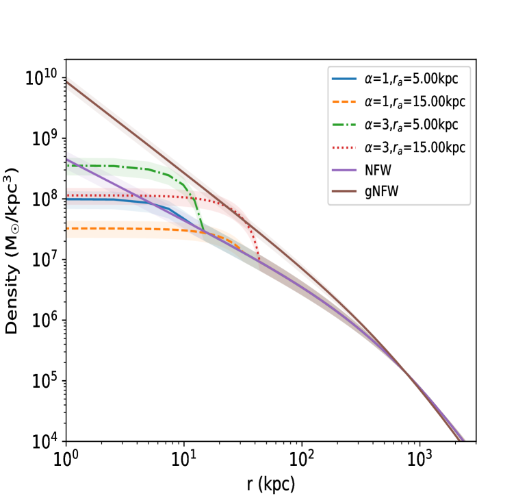
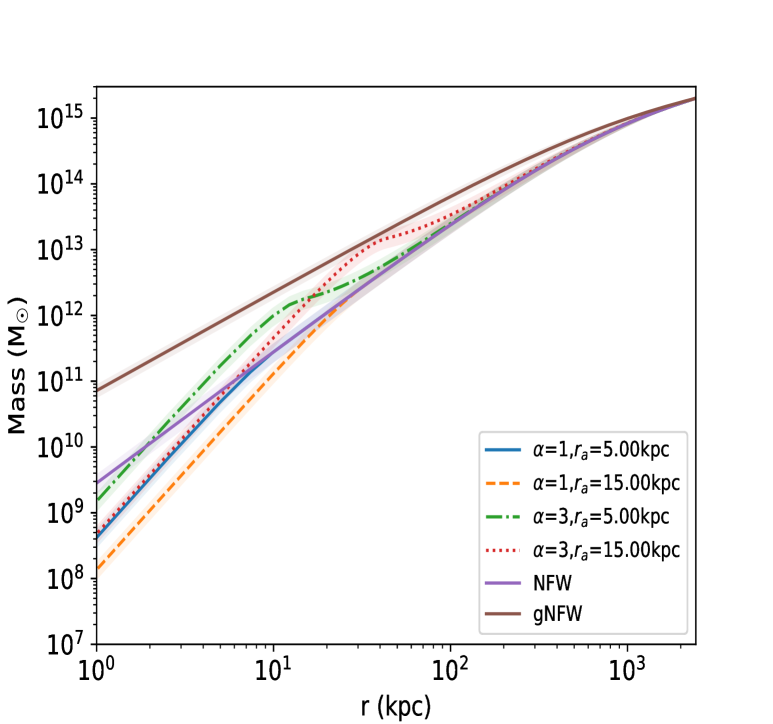
Figure 1: [$M_{h}=2\cdot 10^{15}\rm M_{\odot}$] Left: Density profile of the halo with $M_{h}=2\cdot 10^{15}\rm M_{\odot}$, showing the impact of the solitonic core at small scales and the recovery of the NFW behavior at larger radii. NFW profile in purple solid line for reference.Right: Mass profile of the halo with $M_{h}=2\cdot 10^{15}\rm M_{\odot}$. The soliton’s contribution is evident at small radii but remains negligible in the total mass at larger scales. NFW profile in purple solid line for reference.

Figure 1 illustrates the density and mass profiles, respectively for these configurations. Moreover, we present the profile of the generalized NFW model (gNFW), given that the applicability of the standard NFW profile in the central regions of halos remains debated due to observational discrepancies, frequently attributed to baryonic processes that can significantly influence the density profile near the core. Further details on this profile can be found in Appendix B.

For profiles with solitonic contributions, increasing $\alpha$ at fixed $r_{a}$ enhances central densities $\rho_{c}$, soliton masses $M_{\rm sol}$, and fractional mass contributions $f_{\rm sol}$. For example, at $r_{a}=5\,\mathrm{kpc}$, $\alpha=3$ yields $\rho_{c}=3.64\cdot 10^{8}\,\mathrm{M_{\odot}/kpc^{3}}$ and $M_{\rm sol}=1.75\cdot 10^{12}\,\mathrm{M_{\odot}}$—values significantly higher than those for $\alpha=1$. Conversely, at fixed $\alpha$, increasing $r_{a}$ enlarges the transition radius,$r_{t}$ and $M_{\rm sol}$ while reducing $\rho_{c}$. For $\alpha=1$, raising $r_{a}$ to $15\,\mathrm{kpc}$ boosts $M_{\rm sol}$ to $2.75\cdot 10^{12}\,\mathrm{M_{\odot}}$ but lowers $\rho_{c}$ to $3.26\cdot 10^{7}\,\mathrm{M_{\odot}/kpc^{3}}$. Despite these trends, $f_{\rm sol}$ remains modest, peaking at $0.74\%$ for $\alpha=3$ and $r_{a}=15\,\mathrm{kpc}$. Similarly, the relative change in total halo mass $\Delta M_{h}$ is negligible overall, though marginally larger for higher $\alpha$ and $r_{a}$.

These results highlight the delicate interplay between soliton properties and halo parameters: While solitons shape the central mass distribution, their contribution to the total halo mass remains minor. At large radii, the density profile reverts to the standard NFW form, confirming that solitonic effects are restricted to the core. This behavior aligns with mass conservation principles, as the halo retains its dominant mass fraction outside the soliton-dominated region. The methodology adopted here thus successfully captures the interplay between soliton and halo dynamics while maintaining physical consistency.

IV.3.2 Halo $M_{h}=2\cdot 10^{14}M_{\odot}$

Halo $M=2\cdot 10^{14}\rm M_{\odot}$
$\alpha$	$r_{a}$ (kpc)	$r_{t}$ (kpc)	$\rho_{c}$ ($\rm M_{\odot}/kpc^{3}$)	$M_{sol}$ ($\rm M_{\odot}$)	$f_{sol}(\%)$	$\Delta M_{h}\%$
1	5	11.21	$6.20\cdot 10^{7}$	$2.12\cdot 10^{11}$	0.11	0
1	15	33.94	$1.8\cdot 10^{7}$	$1.74\cdot 10^{12}$	0.87	0
3	5	14.50	$2.18\cdot 10^{8}$	$1.05\cdot 10^{12}$	0.52	0.34
3	15	43.36	$6.30\cdot 10^{7}$	$8.15\cdot 10^{12}$	4.08	2.71

Table 3: Parameters of the solitonic profile for the halo of $M_{h}=2\cdot 10^{14}\rm M_{\odot}$, showing the central density, soliton mass, and fractional contribution to the system for different SI-SFDM models and $\alpha$ configurations.

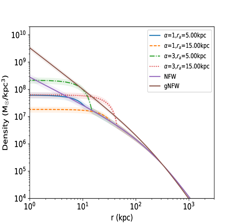
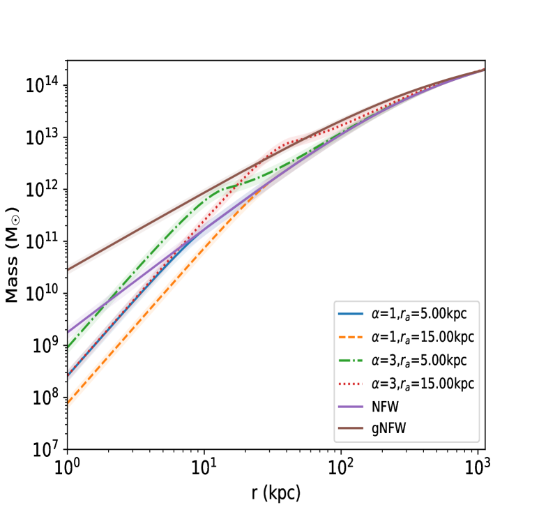
Figure 2: [$M_{h}=2\cdot 10^{14}\rm M_{\odot}$] Left: Density profile for the halo with $M_{h}=2\cdot 10^{14}\rm M_{\odot}$. The soliton’s effect is more prominent in the central regions of the halo.NFW profile in purple solid line for reference.Right: Mass profile for the halo with $M_{h}=2\cdot 10^{14}\rm M_{\odot}$. The soliton’s contribution increases with $\alpha$, but the system retains the overall halo mass structure. NFW profile in purple solid line for reference.

We now analyze the halo of mass $M_{h}=2\cdot 10^{14}M_{\odot}$, incorporating the self-interacting solitonic core. Table 3 summarizes the configuration parameters (matching those in Table 2), which quantify the soliton’s influence on the halo’s density and mass profiles as $\alpha$ and $r_{a}$ vary. Figure 2 illustrates the density and mass profiles, respectively for these configurations.

Consistent with earlier results, increasing $\alpha$ at fixed $r_{a}$ amplifies soliton properties: $\rho_{c}$, $M_{\rm sol}$, and $f_{\rm sol}$ rise sharply (e.g., $\rho_{c}$ increases by a factor of $\sim 3.5$ when $\alpha$ increases from 1 to 3 at $r_{a}=5\,\mathrm{kpc}$). Conversely, increasing $r_{a}$ at fixed $\alpha$ enlarges $r_{t}$ and $M_{\rm sol}$ but suppresses $\rho_{c}$ (e.g., for $\alpha=1$, $r_{a}=15\,\mathrm{kpc}$ reduces $\rho_{c}$ by $\sim 71\%$ compared to $r_{a}=5\,\mathrm{kpc}$).

The fractional contribution of the soliton to the halo mass and the relative grow with $\alpha$ and $r_{a}$. For $\alpha=3$ and $r_{a}=15\,\mathrm{kpc}$, $f_{\rm sol}=4.08\%$ and $\Delta M_{h}=2.71\%$, indicating non-negligible mass redistribution in the core. Compared to the higher-mass halo ($M_{h}=2\times 10^{15}\,\mathrm{M_{\odot}}$), soliton effects are more pronounced here, though total mass conservation remains robust (e.g., $\Delta M_{h}<3\%$ even for maximal $\alpha,r_{a}$).

Figures 1 and 2 confirm the dual-regime structure: soliton-dominated cores transition smoothly to NFW-like profiles at larger radii.The mass profile further confirms that, even with a more pronounced soliton component, the halo structure at larger radii remains dominated by the underlying NFW profile. The method used to describe the system thus proves effective in handling halos with different mass scales, ensuring that the soliton’s impact is accurately modeled while preserving the consistency of the overall mass distribution.

V Lensing estimators for the self-interacting profile

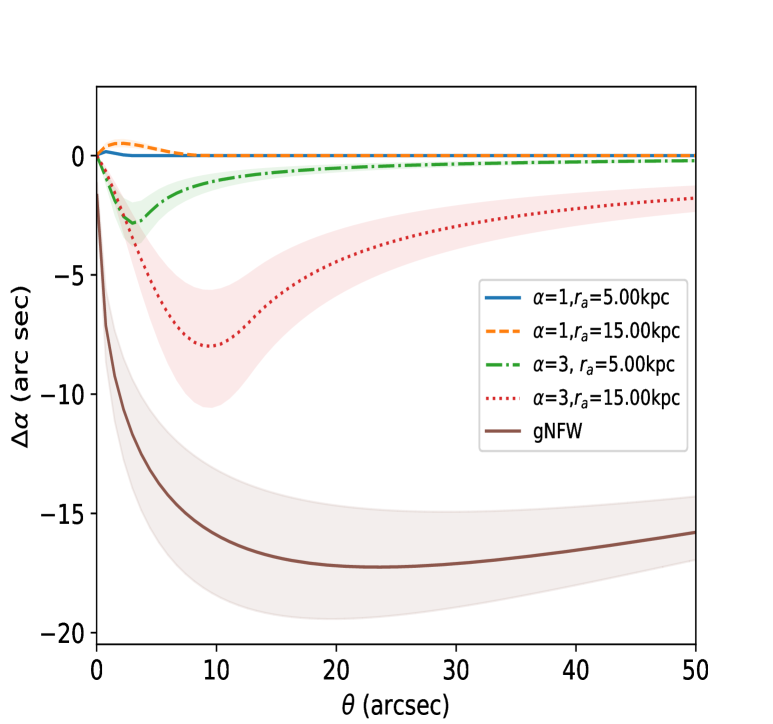
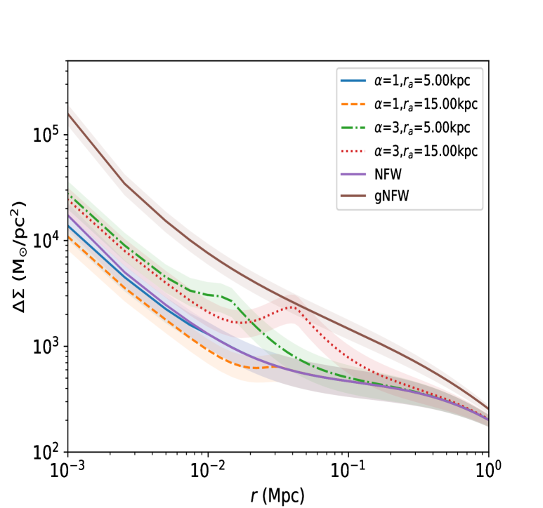
Figure 3: [$M_{h}=2\cdot 10^{15}M_{\odot}$] Left: Difference in deflection angle ($\alpha_{\text{NFW}}-\alpha_{\text{sol}}$) relative to the NFW profile for different soliton configurations. The brown line represents the difference for the gNFW case $\alpha_{\text{NFW}}-\alpha_{\text{gNFW}}$. Right: Excess of surface mass density. Brown line corresponds to the gNFW calculation.

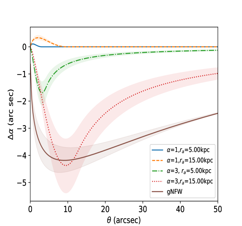
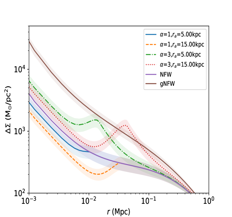
Figure 4: [$M_{h}=2\cdot 10^{14}\rm M_{\odot}$] Left: Difference in deflection angle ($\alpha_{\text{NFW}}-\alpha_{\text{sol}}$) relative to the NFW profile for different soliton configurations. The brown line represents the difference for the gNFW case $\alpha_{\text{NFW}}-\alpha_{\text{gNFW}}$. Right: Excess of surface mass density. Brown line corresponds to the gNFW calculation.

We present the calculations of the lensing estimators, focusing on deflection angle differences between the widely-used NFW profile (our baseline model, central to most lensing analyses) and the solitonic profile. We also quantify the excess surface mass density—a robust estimator on large scales—and compare results to the generalized NFW (gNFW) profile.

For the massive halo ($M_{h}=2\times 10^{15}\,\mathrm{M_{\odot}}$), solitonic cores with three times the NFW-equivalent mass produce significant deflection angle differences. At self-interaction scales of $r_{a}=5\,\mathrm{kpc}$ and $r_{a}=15\,\mathrm{kpc}$, deviations exceed 2 arcseconds at projected radii of 10 kpc and 31 kpc, respectively. These offsets surpass observational thresholds for strong lensing systems, indicating that high-resolution campaigns could resolve soliton-driven deviations from pure NFW halos. Notably, SL achieves sub-arcsecond discrimination precision under fixed projected mass constraints (Limousin et al., 2024), making it ideal for testing such scenarios.

A similar trend emerges for a lower-mass halo ($M_{h}=2\times 10^{14}\,\mathrm{M_{\odot}}$): solitons three times more massive than the NFW component generate deflection differences greater than 2 arcseconds at 10 kpc ($r_{a}=5\,\mathrm{kpc}$) and 32 kpc ($r_{a}=15\,\mathrm{kpc}$), offering clear observational discriminators.

However, degeneracies arise when comparing to the gNFW profile (brown curve, Fig.(4). For the ($\alpha=3,r_{a}=15\,\mathrm{kpc}$) configuration, overlapping regions between soliton and gNFW predictions suggest potential observational ambiguities. This highlights the need for multi-probe analyses but also reveals how baryonic contributions—often modeled via gNFW—might mimic or obscure soliton signatures.

The surface mass density excess further underscores this duality. While large-scale ($\gtrsim 0.1\,\mathrm{Mpc}$) results align between soliton and NFW halos, inner regions ($\lesssim 10\,\mathrm{kpc}$) show marked differences. Observational limitations pose challenges: surveys like (McClintock et al., 2018) typically resolve scales $\geq 0.1\,\mathrm{Mpc}$, where soliton contributions are diluted. Nonetheless, our results emphasize that high-resolution lensing data (e.g., from James Webb Space Telescope (Rigby et al., 2023)) could isolate soliton-driven excesses in the core, advancing both dark matter and baryonic feedback studies.

VI Comparison

In this section, we compare the results of our SI-SFDM model with observational and simulation-based studies to validate and contextualize our findings. First, we focus on the most massive halo in our analysis, $M_{h}=2\cdot 10^{15}\rm M_{\odot}$, as systems of this scale are well-represented in the literature and enable robust comparisons. For this purpose, we select the galaxy cluster A2390 at redshift $z=0.229$ (matching our model’s lensing redshift $z_{l}=0.2$), a well-characterized system with properties analogous to our simulated halo.

The halo mass and NFW parameters derived from our model (Table 4) are consistent with the uncertainty ranges reported in (Newman et al., 2013b), which combines strong/weak lensing and stellar kinematic data. While (Newman et al., 2013a) also provides X-ray-based constraints, these are excluded here to maintain consistency with our lensing-centric methodology.

Cluster	$r_{s}$ (kpc)	$c_{200}$	$\log M_{200}/\rm M_{\odot}$	$r_{200}$ (kpc)
A2390	$763^{+119}_{-107}$	$3.24^{+0.35}_{-0.31}$	$15.34^{+0.06}_{-0.07}$	$2470^{+112}_{123}$
$2\cdot 10^{15}\rm M_{\odot}$	$695.24\pm 198.64$	$3.5\pm 1$	$15.30$	$2433.33$

Table 4: Comparison of NFW parameters for A2390 (from (Newman et al., 2013b)) and our SI-SFDM model for $M_{h}=2\cdot 10^{15}\rm M_{\odot}$. Uncertainties for A2390 reflect combined lensing and stellar dynamics.

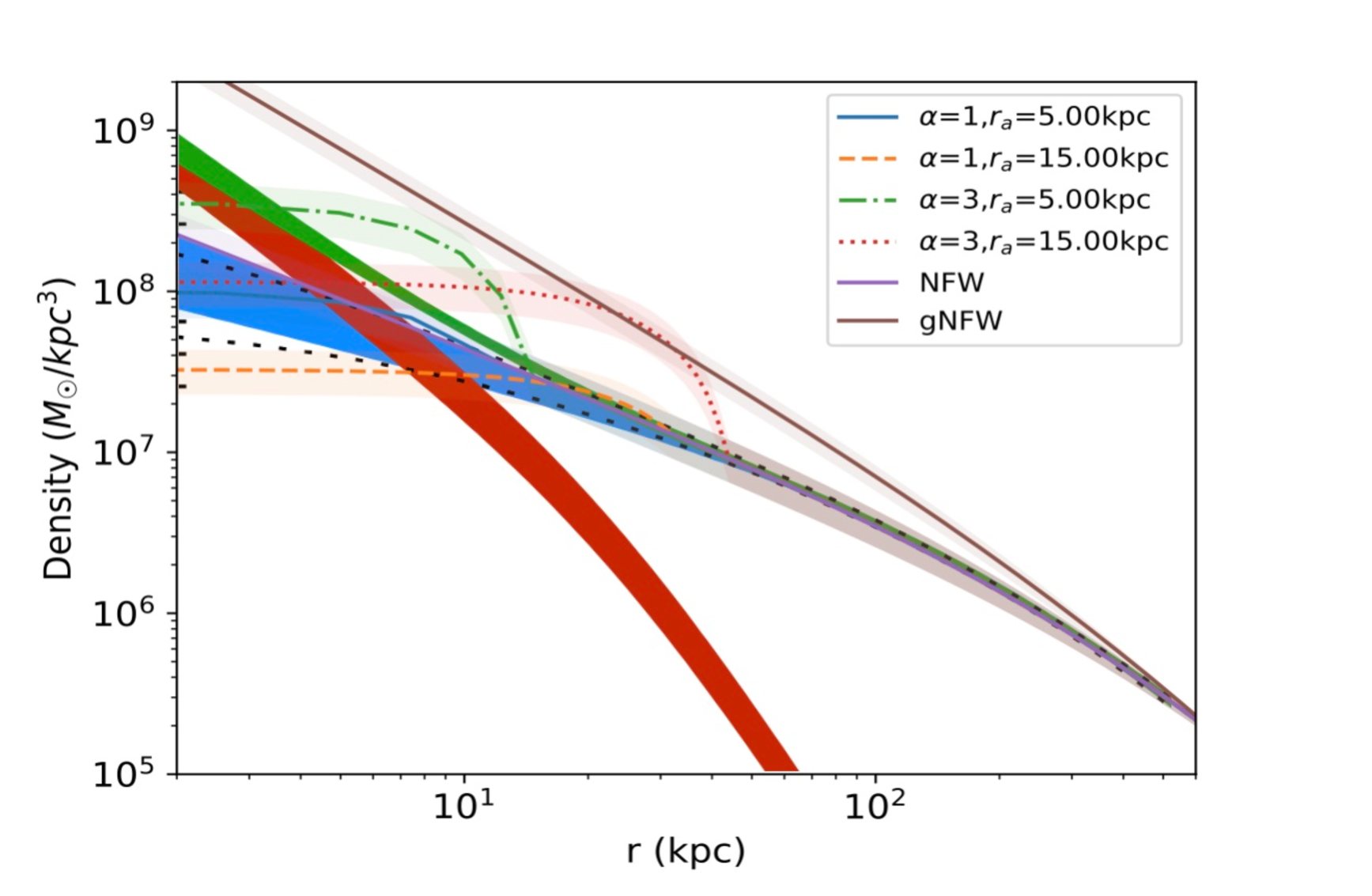
Figure 5: Comparison of the radial density profiles of the SI-SFDM dark matter models for the $M_{h}=2\cdot 10^{15}\rm M_{\odot}$ halo with A2390 observations and simulations from (Newman et al., 2013a). The blue, red, and green bands represent the radial density profiles of the DM halo, the stars in the BCG, and their total in A2390, respectively. The color scheme for the SI-SFDM profiles is consistent with that shown in Fig 1.

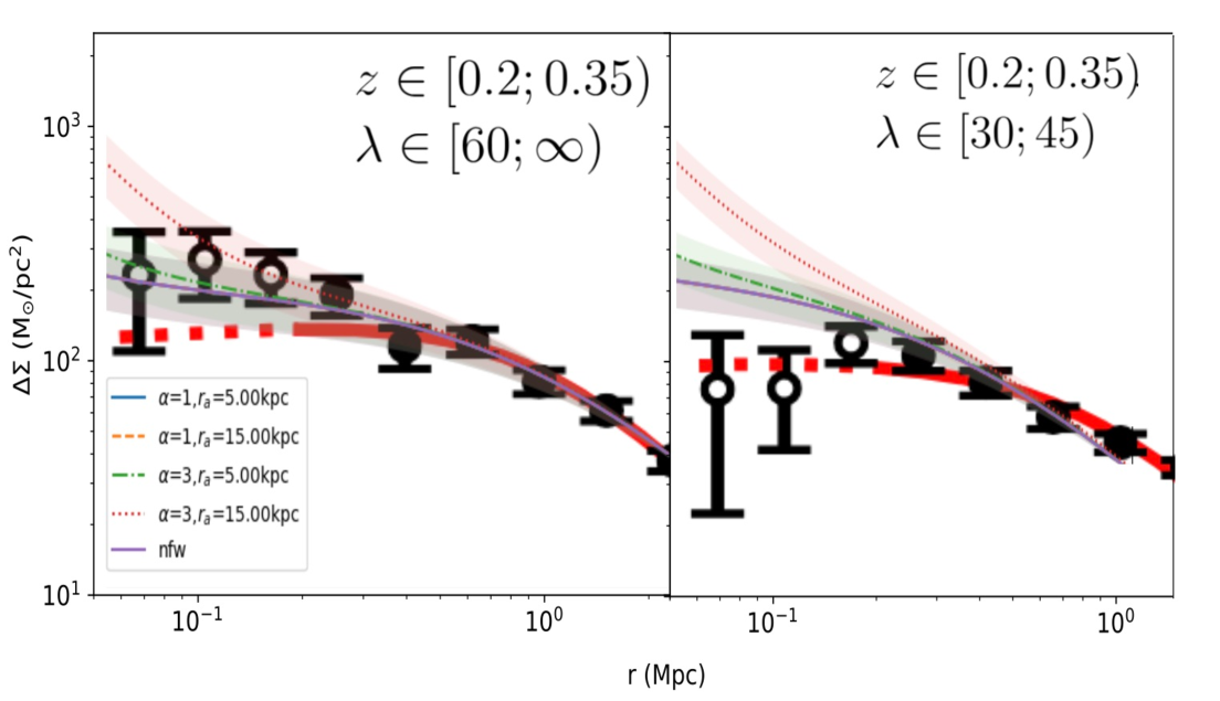
Figure 6: Comparison of excess surface mass density for the halos $M_{h}=2\cdot 10^{15}\rm M_{\odot}$ (left) and $M_{h}=2\cdot 10^{14}\rm M_{\odot}$ (right) with (McClintock et al., 2018).

Figure 5 compares the radial density profiles of our SI-SFDM models with A2390’s profile. The density profile of A2390 includes contributions from dark matter (modeled with generalized NFW [gNFW; light blue] and classical NFW [cNFW; black dashed]), stars in the brightest cluster galaxy (BCG; red), and the total mass (green band).

These components are derived from observations of multiple images, lensing data, and kinematics. In the inner regions ($r\lesssim 5\text{–}10$ kpc), where stars dominate, the total density profile steepens significantly. The stellar mass density in the model of A2390 reaches parity with DM at approximately 7 kpc, while enclosed mass equality occurs at around 12 kpc. Within 5 kpc, the DM fraction is about 25%, increasing to 80% within the three-dimensional half-light radius.

We find that the density profile of the NFW contribution in our model (purple) aligns closely with the corresponding component in A2390’s profile (black-dashed). However, in the inner regions, where the solitonic contribution becomes significant, SI-SFDM models with massive solitons ($\alpha=3$) overpredict densities, suggesting an upper soliton mass limit of $M_{\rm sol}\sim 10^{12}\rm M_{\odot}$. While $\alpha=1$ profiles, where the soliton and NFW masses are equal, match observations, detecting such solitons remains challenging due to their sub-arcsecond angular scales.

We further compare our model’s predictions for the halos studied in this work—located at redshift $z_{l}=0.2$ with masses $M_{h}=2\cdot 10^{15}\rm M_{\odot}$ and $M_{h}=2\cdot 10^{14}\rm M_{\odot}$-to weak lensing results from (McClintock et al., 2018) for the excess surface mass density $\Delta\Sigma$, as shown in Figure 6. The authors in (McClintock et al., 2018) constrain the mass-richness scaling relation of redMaPPer galaxy clusters in the Dark Energy Survey Year 1 data, deriving mean $\Delta\Sigma$ profiles for cluster subsets binned by photometric redshift ($z_{l}$) and optical richness ($\lambda$) of red galaxies. Their analysis excludes scales $r<200$ kpc (open symbols, dashed lines) to avoid contamination from poorly constrained baryonic effects and miscentering.

In Figure 6, the red line represents the best-fit model to the McClintock et al. (2018) data, while our soliton+NFW predictions (color scheme consistent with earlier figures) are overlaid. The right panel corresponds to $M_{h}=2\cdot 10^{15}\rm M_{\odot}$ and left panel corresponds to $M_{h}=2\cdot 10^{14}\rm M_{\odot}$. At large scales, our results for $M_{h}=2\cdot 10^{15}\rm M_{\odot}$ and $M_{h}=2\cdot 10^{14}\rm M_{\odot}$ align closely with both observations and the fiducial model from (McClintock et al., 2018), validating the soliton’s negligible impact on the halo outskirts and reinforcing the NFW-like behavior of the total mass profile at these scales. However, in the inner regions, for $M_{h}=2\cdot 10^{15}\rm M_{\odot}$, our model better matches the excluded inner data points than the fiducial model, hinting that solitonic cores in SI-SFDM may resolve small-scale discrepancies. For $M_{h}=2\cdot 10^{14}\rm M_{\odot}$, our predictions agree with data deemed reliable (filled symbols) but diverge at $r<200$ kpc, underscoring the need for improved observational resolution.

This discrepancy underscores a key challenge: while soliton-driven deviations are most significant in the core, observational limitations currently preclude their direct detection in weak lensing data. The agreement at larger radii, however, demonstrates that our soliton+NFW framework preserves the established success of NFW-based lensing models on scales where baryonic uncertainties dominate. Future efforts combining JWST’s resolution (probing $r<200$ kpc) with wide-field surveys like Rubin Observatory could bridge this gap, testing soliton predictions while refining mass-richness calibration. Similarly, advances in stellar kinematics may resolve the $\alpha=1$ soliton regime, offering a critical test for scalar field dark matter.

VII Conclusion

The distinct gravitational lensing signatures arising from differences between cold dark matter and self-interacting scalar field dark matter density profiles provide a critical observational avenue to test these competing models. Our analysis demonstrates that SI-SFDM parameters can be effectively constrained using existing lensing data, advancing our understanding of dark matter’s fundamental properties. Specifically, our results align with weak lensing mass calibrations at large scales from (McClintock et al., 2018), validating the robustness of our methodology. Comparisons with the multi-probe lensing and stellar dynamics analysis of A2390 by Newman et al. (2013b) further reinforce the viability of SI-SFDM, showing strong concordance in halo parameters such as mass and concentration. Additionally, for the most massive halo ($M_{h}=2\times 10^{15}\,\rm M_{\odot}$), we establish an upper soliton mass limit of $M_{\rm sol}\sim 10^{12}\,\rm M_{\odot}$ in configurations with $\alpha=3$ and $r_{a}=5\,\rm kpc$ and $r_{a}=15\,\rm kpc$, refining the parameter space for solitonic cores.

To strengthen these results, we propose a two-pronged approach for future work. First, we will incorporate solitonic profiles into analyses of observed multiple-image lensing systems, directly applying our model to real data. By initially neglecting error propagation, we aim to prioritize model discrimination and statistically robust comparisons, testing whether SI-SFDM can explain lensing features as a viable alternative to CDM. This approach will enable simulations of lensed images across SI-SFDM scenarios, probing whether input soliton parameters (e.g., $\alpha$, $r_{a}$) can be accurately reconstructed from synthetic and observational data. Second, we will rigorously evaluate whether real data supports solitons as unique descriptors of halo cores or if degeneracies arise with other mass components. These efforts will focus on the central regions of galaxy clusters, where SI-SFDM deviations from CDM predictions are most pronounced, offering a direct test of scalar field dynamics on small scales.

Future initiatives combining Euclid, JWST’s resolution with wide-field surveys like Rubin Observatory will play a pivotal role in advancing this work. Their improved resolution and sensitivity will enable tests of SI-SFDM predictions at sub-arcsecond scales, particularly for low-mass solitons ($\alpha=1$). These efforts will ultimately clarify whether self-interacting scalar fields represent a fundamental component of the dark sector or if new physics beyond current paradigms must be invoked.

Appendix A Self-interacting scalar field dark matter vs. Self-interacting dark matter

In this appendix, we discuss the difference in the sign of terms in the Lagrangian between SI-SFDM and SIDM, which stems from the distinct physical frameworks of these models. As we presented, in SI-SFDM, the Lagrangian includes a scalar field $\phi$ with a potential $V(\phi)$, expressed as Eq.(1). The potential Eq.(2) in this case incorporates self-interaction terms like Eq.(3), where the sign of $\lambda_{4}\phi^{4}$ dictates whether the interactions are repulsive $(\lambda_{4}>0)$ or attractive $(\lambda_{4}<0)$. In this work, we study the repulsive interactions $(\lambda_{4}\phi^{4})$ that are frequently used to stabilize the scalar field and counteract gravitational collapse, whereas attractive terms might be explored for clumping or other effects.

In contrast, SIDM involves particle interactions mediated by a new force, often described by Yukawa couplings (Tulin and Yu, 2018). The Lagrangian includes terms like

$$\mathcal{L}_{\text{SIDM}}=g_{\chi}\bar{\chi}\chi\phi,$$ (32)

in the scalar case, where $\chi$ is the particle DM, $\phi$ represents a mediator and $g_{\chi}$ is the coupling constant. In the non-relativistic limit, self-interactions are described by the Yukawa potential.

$$V(r)=\pm\frac{\alpha_{\chi}}{r}e^{-m_{\phi}r}$$ (33)

Here, the parameters are the dark fine structure constant, $\alpha_{\chi}=\frac{g_{\chi}^{2}}{4\pi},$ the mediator mass $m_{\phi}$, and the dark matter particle mass $m_{\chi}$. The sign of the effective interaction here arises from the nature of the mediator. For a vector mediator, the potential is attractive ($-$) for $\chi\bar{\chi}$ (particle-antiparticle) scattering and repulsive ($+$) for $\chi\chi$ or $\bar{\chi}\bar{\chi}$ scattering. For a scalar mediator, the potential is purely attractive. These interactions influence key physical properties, such as core formation in dark matter halos. In essence, while the sign of SFDM self-interaction terms is a direct model choice influencing stability and structure formation, the sign in SIDM is tied to mediator dynamics and its impact on interaction cross-sections and halo profiles.

Appendix B Testing the consistency of NFW parameters with a Steeper central density profile

In this appendix, we revisit the NFW profile by introducing a steeper central density profile to investigate how the parameters, particularly the concentration parameter $c_{200}$, change. The NFW profile, commonly used in cosmology to describe the dark matter distribution, assumes a universal structure, but its applicability in the central regions of halos remains debated due to observational tensions. These tensions are often attributed to baryonic effects like AGN feedback and compression, which can significantly impact the density profile near the core.

To account for baryonic compression, we use a steeper profile, inspired by the findings of (Schneider and Teyssier, 2016), that better represents the density in the halo core. This steeper profile is parameterized as:

$$\rho(r)=\frac{\rho_{s}}{\left(\frac{r}{r_{s}}\right)^{\gamma}\left(1+\left(\frac{r}{r_{s}}\right)^{\alpha}\right)^{(\beta-\gamma)/\alpha}}$$ (34)

where the parameters are set to $\alpha=1$ that controls the smoothness of the transition between the inner and outer regions. $\beta=3$ that defines the outer slope, consistent with standard halo profile and $\gamma=1.5$ representing a steeper inner slope than the standard NFW profile ($\gamma=1$). Due to the lack of direct observational constraints on the central regions of halos, this profile is used as a conservative estimate for the potential mass distribution in the core.

In order to recompute the generalized NFW (gNFW) profile with the same concentration and total mass as the NFW profile, it is first necessary to take the same values of the concentration parameter $c_{200}$ and halo mass $M_{200}$. The radius $r_{200}$ is computed from equation (28), and the scale radius, $r_{s}$ is determined with (29). The density scale $\rho_{s}$ is then calculated by imposing that the gNFW profile yields the same total mass as the NFW profile.

This approach is practical, as the mass and concentration of the halo are typically the most directly constrained parameters. This comparison allows us to assess whether the steeper profile introduces significant deviations in the characteristics of the halo or remains consistent with the NFW model.

The results are presented in the following table:

$M_{200}(\rm M_{\odot}$)	$r_{200}$ (kpc)	$c_{200}$	$\rho_{s}(\rm 10^{5}M_{\odot}/kpc^{3}$)	$r_{s}$ (kpc)
$2\cdot 10^{15}$	2433.33	$3.5\pm 1$	$4.71\pm 4.06$	$695.24\pm 198.64$
$2\cdot 10^{14}$	1129.45	$4.5\pm 1$	$8.50\pm 5.69$	$250.99\pm 55.77$

Table 5: Parameters of the gNFW density profile.

The recomputed concentrations for the steeper profile are consistent with those of the standard NFW profile, indicating that while the steeper profile accounts for the possibility of a denser core, the overall halo structure remains well-described by the NFW model at larger radii. This consistency provides a robust foundation for using the NFW profile as the baseline to explore self-interacting scalar field dark matter systems. By incorporating the recomputed parameters, our models can effectively capture potential variations in dark matter distributions while maintaining alignment with large-scale observations.

Appendix C Uncertainty Propagation Expressions in NFW Density and gNFW Profile Parameters

In this appendix we present the expressions used for the error propagation in our calculations for the density profiles:

$$\Delta r_{s}=\frac{r_{200}}{c^{2}}\Delta c$$ (35)

NFW profile:

$$\Delta\rho_{s}=\frac{M_{200}\left(4r_{200}^{2}+3r_{200}r_{s}+3(r_{200}+r_{s})^{2}\ln\left(\frac{r_{s}}{r_{200}+r_{s}}\right)\right)}{4\pi r_{s}^{4}\left(r_{200}+(r_{200}+r_{s})\ln\left(\frac{r_{s}}{r_{200}+r_{s}}\right)\right)^{2}}\Delta r_{s}$$ (36)

gNFW profile:

$$\Delta\rho_{s}=\rho_{s}\Delta r_{s}\left|\frac{3}{2r_{s}}+\frac{9r_{200}}{10r_{s}^{2}}\frac{{}_{2}F_{1}\left(\frac{5}{2},\,\frac{5}{2};\,\frac{7}{2};\,-\frac{r_{200}}{r_{s}}\right)}{{}_{2}F_{1}\left(\frac{3}{2},\,\frac{3}{2};\,\frac{5}{2};\,-\frac{r_{200}}{r_{s}}\right)}\right|$$ (37)

where $\,{}_{2}F_{1}(a,b;c;z)$ is the hypergeometric function defined as the power series:

$${}_{2}F_{1}(a,b;c;z)=\sum_{n=0}^{\infty}\frac{(a)_{n}(b)_{n}}{(c)_{n}}\frac{z^{n}}{n!},$$

where $(q)_{n}$ is the Pochhammer symbol (rising factorial), given by:

$$(q)_{n}=q(q+1)(q+2)\cdots(q+n-1),\quad(q)_{0}=1.$$

References

- Jungman et al. (1995) G. Jungman, M. Kamionkowski, and K. Griest, Physics Report 267, 195 (1995), eprint 9506380, URL http://arxiv.org/abs/hep-ph/9506380http://dx.doi.org/10.1016/0370-1573(95)00058-5.
- Drees et al. (2005) M. Drees, R. Godbole, and P. Roy, Theory and Phenomenology of Sparticles (World Scientific, 2005), URL https://www.worldscientific.com/doi/abs/10.1142/4001.
- Steigman and Turner (1985) G. Steigman and M. S. Turner, Nuclear Physics B 253, 375 (1985), ISSN 0550-3213, URL https://www.sciencedirect.com/science/article/pii/0550321385905371.
- Schumann (2019) M. Schumann, Journal of Physics G Nuclear Physics 46, 103003 (2019), eprint 1903.03026.
- Conrad (2014) J. Conrad, arXiv e-prints arXiv:1411.1925 (2014), eprint 1411.1925.
- Arcadi et al. (2018) G. Arcadi, M. Dutra, P. Ghosh, M. Lindner, Y. Mambrini, M. Pierre, S. Profumo, and F. S. Queiroz, European Physical Journal C 78, 203 (2018), eprint 1703.07364.
- Weinberg et al. (2015) D. H. Weinberg, J. S. Bullock, F. Governato, R. K. De Naray, and A. H. Peter, Proceedings of the National Academy of Sciences of the United States of America 112, 12249 (2015), ISSN 10916490, eprint 1306.0913.
- Del Popolo and Delliou (2016) A. Del Popolo and M. L. Delliou, Galaxies 5 (2016), eprint 1606.07790, URL http://arxiv.org/abs/1606.07790http://dx.doi.org/10.3390/galaxies5010017.
- Nakama et al. (2017) T. Nakama, J. Chluba, and M. Kamionkowski, Physical Review D 95, 121302 (2017), ISSN 24700029, eprint 1703.10559.
- Di Luzio et al. (2020) L. Di Luzio, M. Giannotti, E. Nardi, and L. Visinelli, Physics Reports 870, 1 (2020), eprint 2003.01100, URL http://arxiv.org/abs/2003.01100http://dx.doi.org/10.1016/j.physrep.2020.06.002.
- Hu et al. (2000) W. Hu, R. Barkana, and A. Gruzinov, Phys. Rev. Lett. 85, 1158 (2000), URL https://link.aps.org/doi/10.1103/PhysRevLett.85.1158.
- Hui et al. (2017) L. Hui, J. P. Ostriker, S. Tremaine, and E. Witten, Physical Review D 95, 43541 (2017), URL https://journals.aps.org/prd/abstract/10.1103/PhysRevD.95.043541.
- Goodman (2000) J. Goodman, New Astron. 5, 103 (2000), eprint astro-ph/0003018.
- Lee and Pang (1992) T. D. Lee and Y. Pang, Phys. Rept. 221, 251 (1992).
- Guth et al. (2015) A. H. Guth, M. P. Hertzberg, and C. Prescod-Weinstein, Phys. Rev. D 92, 103513 (2015), eprint 1412.5930.
- Sikivie and Yang (2009) P. Sikivie and Q. Yang, Phys. Rev. Lett. 103, 111301 (2009), eprint 0901.1106.
- Schive et al. (2014a) H. Y. Schive, T. Chiueh, and T. Broadhurst, Nature Physics 10, 496 (2014a), ISSN 17452481, eprint 1406.6586.
- Schive et al. (2014b) H. Y. Schive, M. H. Liao, T. P. Woo, S. K. Wong, T. Chiueh, T. Broadhurst, and W. Y. Hwang, Physical Review Letters 113, 1 (2014b), ISSN 10797114, eprint 1407.7762.
- Galazo-Garc´ıa et al. (2022) R. Galazo-García, P. Brax, and P. Valageas, Phys. Rev. D 105, 123528 (2022), eprint 2203.05995.
- Suárez and Chavanis (2015) A. Suárez and P. H. Chavanis, Physical Review D - Particles, Fields, Gravitation and Cosmology 92, 023510 (2015), ISSN 15502368, URL https://journals.aps.org/prd/abstract/10.1103/PhysRevD.92.023510.
- Brax et al. (2019) P. Brax, J. A. R. Cembranos, and P. Valageas, Phys. Rev. D 100, 023526 (2019), eprint 1906.00730.
- Thomas (1927) L. H. Thomas, Mathematical Proceedings of the Cambridge Philosophical Society 23, 542–548 (1927).
- Chavanis (2011) P.-H. Chavanis, Phys. Rev. D 84, 043531 (2011), eprint 1103.2050.
- Chavanis (2018) P.-H. Chavanis, Phys. Rev. D 98, 023009 (2018), eprint 1710.06268.
- Dawoodbhoy et al. (2021) T. Dawoodbhoy, P. R. Shapiro, and T. Rindler-Daller, Mon. Not. Roy. Astron. Soc. 506, 2418 (2021), eprint 2104.07043.
- Shapiro et al. (2021) P. R. Shapiro, T. Dawoodbhoy, and T. Rindler-Daller, Mon. Not. Roy. Astron. Soc. 509, 145 (2021), eprint 2106.13244.
- Suárez and Chavanis (2017) A. Suárez and P. H. Chavanis, Physical Review D 95, 063515 (2017), ISSN 24700029, URL https://journals.aps.org/prd/abstract/10.1103/PhysRevD.95.063515.
- Li et al. (2014) B. Li, T. Rindler-Daller, and P. R. Shapiro, Physical Review D - Particles, Fields, Gravitation and Cosmology 89, 083536 (2014), ISSN 15502368, URL https://journals.aps.org/prd/abstract/10.1103/PhysRevD.89.083536.
- Nori and Baldi (2018) M. Nori and M. Baldi, Mon. Not. Roy. Astron. Soc. 478, 3935 (2018), eprint 1801.08144.
- Galazo García et al. (2024) R. Galazo García, P. Brax, and P. Valageas, Phys. Rev. D 109, 043516 (2024), URL https://link.aps.org/doi/10.1103/PhysRevD.109.043516.
- Galazo García et al. (2025) R. Galazo García, P. Brax, and P. Valageas, Phys. Rev. D 111, 063511 (2025), URL https://link.aps.org/doi/10.1103/PhysRevD.111.063511.
- Brax and Valageas (2025a) P. Brax and P. Valageas (2025a), eprint 2501.02297.
- Brax and Valageas (2025b) P. Brax and P. Valageas (2025b), eprint 2502.12100.
- Boudon et al. (2023) A. Boudon, P. Brax, P. Valageas, and L. K. Wong, Physical Review D 109 (2023), ISSN 24700029, eprint 2305.18540, URL https://arxiv.org/abs/2305.18540v3.
- Bar et al. (2019) N. Bar, K. Blum, T. Lacroix, and P. Panci, Journal of Cosmology and Astroparticle Physics 2019, 045–045 (2019), ISSN 1475-7516, URL http://dx.doi.org/10.1088/1475-7516/2019/07/045.
- Chakrabarti et al. (2022) S. Chakrabarti, B. Dave, K. Dutta, and G. Goswami, Journal of Cosmology and Astroparticle Physics 2022, 074 (2022), ISSN 1475-7516, URL http://dx.doi.org/10.1088/1475-7516/2022/09/074.
- Gómez and Valageas (2024) G. Gómez and P. Valageas, Phys. Rev. D 109, 103038 (2024), URL https://link.aps.org/doi/10.1103/PhysRevD.109.103038.
- Sand et al. (2004) D. J. Sand, T. Treu, G. P. Smith, and R. S. Ellis, Astrophys. J. 604, 88 (2004).
- Newman et al. (2013a) A. B. Newman, T. Treu, R. S. Ellis, D. J. Sand, C. Nipoti, J. Richard, and E. Jullo, The Astrophysical Journal 765, 24 (2013a), ISSN 1538-4357, URL http://dx.doi.org/10.1088/0004-637X/765/1/24.
- Limousin et al. (2022) M. Limousin, B. Beauchesne, and E. Jullo, Astronomy & Astrophysics 664, A90 (2022), ISSN 1432-0746, URL http://dx.doi.org/10.1051/0004-6361/202243278.
- Limousin et al. (2008) M. Limousin, J. Richard, J.-P. Kneib, H. Brink, R. Pelló, E. Jullo, H. Tu, J. Sommer-Larsen, E. Egami, M. J. Michałowski, et al., Astronomy & Astrophysics 489, 23–35 (2008), ISSN 1432-0746, URL http://dx.doi.org/10.1051/0004-6361:200809646.
- Sirks et al. (2024) E. L. Sirks, D. Harvey, R. Massey, K. A. Oman, A. Robertson, C. Frenk, S. Everett, A. S. Gill, D. Lagattuta, and J. McCleary, Monthly Notices of the Royal Astronomical Society 530, 3160 (2024), eprint 2405.00140.
- Randall et al. (2008) S. W. Randall, M. Markevitch, D. Clowe, A. H. Gonzalez, and M. Bradač, Astrophys. J. 679, 1173 (2008), eprint 0704.0261.
- Harvey et al. (2015) D. Harvey, R. Massey, T. Kitching, A. Taylor, and E. Tittley, Science 347, 1462–1465 (2015), ISSN 1095-9203, URL http://dx.doi.org/10.1126/science.1261381.
- Beauchesne et al. (2024) B. Beauchesne, B. Clément, P. Hibon, M. Limousin, D. Eckert, J.-P. Kneib, J. Richard, P. Natarajan, M. Jauzac, M. Montes, et al., Monthly Notices of the Royal Astronomical Society 527, 3246 (2024), eprint 2301.10907.
- Massey et al. (2010) R. Massey, T. Kitching, and J. Richard, Reports on Progress in Physics 73, 086901 (2010), ISSN 1361-6633, URL http://dx.doi.org/10.1088/0034-4885/73/8/086901.
- Tulin and Yu (2018) S. Tulin and H.-B. Yu, Physics Reports 730, 1–57 (2018), ISSN 0370-1573, URL http://dx.doi.org/10.1016/j.physrep.2017.11.004.
- Navarro et al. (1997) J. F. Navarro, C. S. Frenk, and S. D. M. White, The Astrophysical Journal 490, 493–508 (1997), ISSN 1538-4357, URL http://dx.doi.org/10.1086/304888.
- Limousin et al. (2024) M. Limousin, B. Beauchesne, A. Niemiec, J. M. Diego, M. Jauzac, A. Koekemoer, K. Sharon, A. Acebron, D. Lagattuta, G. Mahler, et al., Astronomy & Astrophysics 693, A33 (2024), ISSN 1432-0746, URL http://dx.doi.org/10.1051/0004-6361/202451969.
- Madelung and Frankfurt (1926) E. Madelung and I. Frankfurt, Ann. d. Phys 79 (1926).
- Seidel and Suen (1994) E. Seidel and W. M. Suen, Physical Review Letters 72, 2516 (1994), ISSN 00319007, URL /prl/abstract/10.1103/PhysRevLett.72.2516.
- Chavanis and Delfini (2011) P. H. Chavanis and L. Delfini, Phys. Rev. D 84, 43532 (2011), eprint 1103.2054.
- Harko (2011) T. Harko, Mon. Not. Roy. Astron. Soc. 413, 3095 (2011), eprint 1101.3655.
- Einstein (1936) A. Einstein, Science 84, 506 (1936).
- Schneider et al. (1992) P. Schneider, J. Ehlers, and E. E. Falco, Gravitational Lenses (Springer Berlin, Heidelberg, 1992).
- Narayan and Bartelmann (1997) R. Narayan and M. Bartelmann, Lectures on gravitational lensing (1997), eprint astro-ph/9606001, URL https://arxiv.org/abs/astro-ph/9606001.
- Meneghetti (2021) M. Meneghetti, Introduction to Gravitational Lensing: With Python Examples, Lecture Notes in Physics (Springer International Publishing, 2021), ISBN 9783030735821, URL https://books.google.es/books?id=2HlMEAAAQBAJ.
- Bartelmann and Schneider (2001) M. Bartelmann and P. Schneider, Physics Reports 340, 291–472 (2001), ISSN 0370-1573, URL http://dx.doi.org/10.1016/S0370-1573(00)00082-X.
- Suárez and Chavanis (2016) A. Suárez and P.-H. Chavanis, Physical Review D 95 (2016), eprint 1608.08624, URL http://arxiv.org/abs/1608.08624http://dx.doi.org/10.1103/PhysRevD.95.063515.
- Schwabe et al. (2016) B. Schwabe, J. C. Niemeyer, and J. F. Engels, Physical Review D 94, 43513 (2016), ISSN 24700029, eprint 1606.05151, URL https://journals.aps.org/prd/abstract/10.1103/PhysRevD.94.043513.
- Ishiyama et al. (2020) T. Ishiyama, F. Prada, A. A. Klypin, M. Sinha, R. B. Metcalf, E. Jullo, B. Altieri, S. A. Cora, D. Croton, S. de la Torre, et al., Monthly Notices of the Royal Astronomical Society 506, 4210 (2020), eprint 2007.14720v3, URL http://arxiv.org/abs/2007.14720http://dx.doi.org/10.1093/mnras/stab1755.
- McClintock et al. (2018) T. McClintock, T. N. Varga, D. Gruen, E. Rozo, E. S. Rykoff, T. Shin, P. Melchior, J. DeRose, S. Seitz, J. P. Dietrich, et al., Monthly Notices of the Royal Astronomical Society 482, 1352–1378 (2018), ISSN 1365-2966, URL http://dx.doi.org/10.1093/mnras/sty2711.
- Rigby et al. (2023) J. Rigby, M. Perrin, M. McElwain, R. Kimble, S. Friedman, M. Lallo, R. Doyon, L. Feinberg, P. Ferruit, A. Glasse, et al., Publications of the Astronomical Society of the Pacific 135, 048001 (2023), ISSN 1538-3873, URL http://dx.doi.org/10.1088/1538-3873/acb293.
- Newman et al. (2013b) A. B. Newman, T. Treu, R. S. Ellis, and D. J. Sand, The Astrophysical Journal 765, 25 (2013b), ISSN 1538-4357, URL http://dx.doi.org/10.1088/0004-637X/765/1/25.
- Schneider and Teyssier (2016) A. Schneider and R. Teyssier (2016), eprint 1510.06034v2, URL www.lsst.org/lsst.