Deterministic generation of multi-qubit entangled states among distant parties using indefinite causal order

Abstract

Quantum entanglement plays an irreplaceable role in various remote quantum information processing tasks. Here we present protocols for generating deterministic and heralded $N$-qubit entangled states across multiple network nodes. By utilizing a pre-shared maximally entangled state and single-qubit operations within an indefinite causal order framework, the multi-qubit entangled state between distant parties can be generated deterministically. The complex entangled state measurements and multiple pre-shared entangled states, are essential in conventional entanglement swapping technique, but are not required in our approach. This greatly reduces the complexity of the quantum circuit and makes it more experimentally feasible. Furthermore, we develop optical architectures to implement these protocols by encoding qubits in polarization degree of freedom. The results indicate that our protocols significantly improve the efficiency of long-distance entanglement generation and provide a practical framework for establishing large-scale quantum networks.

I Introduction

Quantum entanglement Horodecki et al. (2009) over long-distance quantum network nodes is a key resource for implementing distributed quantum computing Jiang et al. (2007); Oh et al. (2023); Liu et al. (2024a), quantum secure communication Long and Liu (2002); Xu et al. (2020); Sheng et al. (2022); Zhou and Sheng (2022); Zhou et al. (2023a); Zhao et al. (2024), quantum nonlocal correlations Chaturvedi et al. (2024); Villegas-Aguilar et al. (2024); Lobo et al. (2024), and quantum metrology Yin et al. (2020); Zhao et al. (2021); Malia et al. (2022). Nowadays, many works have been proposed for generating entangled states Wang et al. (2018); Chen et al. (2024); Cao et al. (2024). However, these theoretical and experimental works primarily focus on qubit-based local systems, while long-distance entanglement states remains relatively scarce. Entanglement swapping is a well-known technique to create long-distance entanglement between two remote particles Pan et al. (1998); de Riedmatten et al. (2005); Su et al. (2016). By utilizing two pre-shared entangled pairs and an appropriate entanglement measurement (such as, Bell state measurement), entangled states between two distant qubits can be generated.

Over the past two decades, entanglement swapping has been experimentally demonstrated across various physical platforms, including all-photonic systems Pan et al. (1998); Liu et al. (2022), atoms Chou et al. (2007), trapped ions Riebe et al. (2008), quantum dots Zopf et al. (2019), and superconducting circuits Ning et al. (2019). The primary challenges in entanglement swapping lie in the efficient generation of entangled photon pairs and the implementation of Bell state measurement (BSM). First, the generation efficiency of entangled photon pairs using spontaneous parametric down-conversion (SPDC) is inherently low Couteau (2018). Second, the probabilistic character of BSM is unavoidable in linear optical systems without additional resources or assistance Lütkenhaus et al. (1999); Calsamiglia and Lütkenhaus (2001); Bayerbach et al. (2023). To completely distinguish all Bell states, strategies such as utilizing additional degrees of freedom (DoFs) Walborn et al. (2003); Barbieri et al. (2007); Williams et al. (2017); Zhou et al. (2022), or additional entanglement, or nonlinear media Sheng et al. (2010); Li and Ghose (2016); Li et al. (2019) are usually adopted. However, these approaches are challenged by inefficiency and impracticality.

Besides the quantum swapping technique, a quantum bus assisted by auxiliary photons provides an alternative approach for creating remote multi-qubit entanglement Callus and Kok (2021); Li et al. (2018, 2016); Sangouard et al. (2011); Munro et al. (2012); Wu et al. (2022); Xie et al. (2023); Zhou et al. (2023b); Li et al. (2024). In this approach, a hybrid entanglement between a stationary qubit and a photon qubit is established at each node, followed by photon-photon interactions at an intermediate node Callus and Kok (2021) or photon-spin interactions at another node Li et al. (2018). After appropriate measurements are made on auxiliary photons, the system will automatically collapse into an entangled state. Unfortunately, such multi-qubit entanglement is degraded by the channel noise and photon loss, because the numerous single photons or entangled photon pairs need to travel in long-distance optical fibers or free-space channels Li et al. (2016); Sangouard et al. (2011); Munro et al. (2012); Wu et al. (2022). In 2019, Piparo et al. Lo Piparo et al. (2019) proposed quantum multiplexing to improve the efficiency of the long-distance entanglement generation. Later, some intriguing protocols utilizing an entangled photon pair Xie et al. (2023) or a single photon as a quantum bus Zhou et al. (2023b); Li et al. (2024) have been proposed to improve the efficiency of multiple entangled pairs. Long-distance quantum entanglement has been experimentally demonstrated in various systems Bernien et al. (2013); van Leent et al. (2022); Krutyanskiy et al. (2023), but the limited photon transmission rate restricts the efficiency of the multi-qubit long-distance entanglement generation.

In this paper, we present alternative protocols for deterministically generating an $N$-qubit entangled state among $N$ spatially separated parties over long distances within an indefinite causal order (ICO) framework. ICO, a fascinating resource, shows significant advantages over fixed causal order approaches in various quantum information processing tasks Wei et al. (2019); Nie et al. (2022); Yin et al. (2023); Liu et al. (2024b); Liu and Wei (2025). It is known that ICO is realized through quantum switch, and quantum switch has been demonstrated both theoretically Chiribella et al. (2013, 2021); Kechrimparis et al. (2024) and experimentally Procopio et al. (2015); Goswami et al. (2018); Guo et al. (2020); Strömberg et al. (2023); Rozema et al. (2024). Our protocol begins with a pre-shared $N$-qubit maximally entangled state as the control qubits and one single particle held by each party as the target qubits. Then, each party employs the control qubits to manipulate the order of single-qubit gates on their respective target qubits. Finally, by measuring the control qubits and adjusting an angle of the single-qubit rotation gates, the system can collapse into a maximally entangled state (MES), or a partially entangled state (PES), or a separable state (SS). In entanglement swapping techniques, which require many pre-shared entangled pairs and complex joint measurements Pan et al. (1998); de Riedmatten et al. (2005); Su et al. (2016); Liu et al. (2022); Chou et al. (2007); Riebe et al. (2008); Zopf et al. (2019); Ning et al. (2019), our protocols rely solely on a pre-shared entanglement, the superposition of simple single-qubit gate orders, and straightforward single-qubit measurements. The approach eliminates the need for multiple entangled states and complex entangled state measurements, thereby reducing both resource requirements and measurement complexity. These advantages make our protocols more practical for the implementation of remote entanglement generation. Additionally, we develop an optical architecture to implement the protocols by utilizing the polarization and path DoFs of single photons. The efficiency of these protocols for $N=3$ and $N=4$ achieve exponential improvements.

II Entangled state generation between multiple long-distance qubits

II.1 Entangled state generation between two long-distance qubits

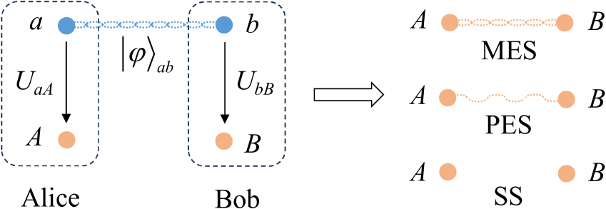
Figure 1: Schematic diagram for generating a general two-qubit quantum state on two remote particles $A$ and $B$. First, a maximally entangled state $|\varphi\rangle_{ab}=\frac{1}{\sqrt{2}}(|0\rangle_{a}|0\rangle_{b}+|1\rangle_{a}|1\rangle_{b})$ is shared with Alice and Bob, and Alice and Bob possess qubits $a$ and $A$, and $b$ and $B$, respectively. Then, Alice performs a two-qubit unitary operation $U_{aA}$ on qubits $a$ and $A$, and Bob performs a two-qubit unitary operation $U_{bB}$ on qubits $b$ and $B$, respectively. Lastly, the qubits $a$ and $b$ are measured in the basis $\{|+\rangle,|-\rangle\}$ and qubits $A$ and $B$ will automatically become a general two-qubit quantum state, i.e., a MES, or a PES, or a SS.

Suppose that Alice and Bob possess particle $A$ and $B$, respectively, and they are initially prepared in the arbitrary states

$$|\psi\rangle_{A}=\sqrt{\alpha_{A}}|0\rangle_{A}+\sqrt{1-\alpha_{A}}|1\rangle_{A},$$ (1)

$$|\psi\rangle_{B}=\sqrt{\alpha_{B}}|0\rangle_{B}+\sqrt{1-\alpha_{B}}|1\rangle_{B}.$$ (2)

Here the coefficients $\alpha_{A},\alpha_{B}\in[0,1]$. Alice and Bob would like to change a given quantum state $|\psi\rangle_{A}\otimes|\psi\rangle_{B}$ to obtain a general two-qubit state, i.e., a MES, or a PES, or a SS.

Figure 1 shows our protocol for creating a general state between two long-distance qubits $A$ and $B$ from a product state $|\psi\rangle_{A}\otimes|\psi\rangle_{B}$. Our protocol can be completed by the following steps.

First, a maximally entangled state

$$|\varphi\rangle_{ab}=\frac{1}{\sqrt{2}}(|0\rangle_{a}|0\rangle_{b}+|1\rangle_{a}|1\rangle_{b}),$$ (3)

is shared with Alice and Bob. The subscripts $a$ and $b$ denote that the qubits $a$ and $b$ are sent to Alice and Bob, respectively. Thus, Alice possesses qubits $a$ and $A$, and Bob possesses qubits $b$ and $B$. The initial state of composite system composed of qubits $a$, $b$, $A$ and $B$ is given by

$$\begin{split}|\Phi_{0}\rangle=&\;|\varphi\rangle_{ab}\otimes|\psi\rangle_{A}\otimes|\psi\rangle_{B}\\ =&\;\frac{1}{\sqrt{2}}(|0\rangle_{a}|0\rangle_{b}+|1\rangle_{a}|1\rangle_{b})\otimes|\psi\rangle_{A}\otimes|\psi\rangle_{B}.\end{split}$$ (4)

Second, Alice (Bob) applies a local two-qubit gate $U_{aA}$ ($U_{bB}$) on qubits $a$ and $A$ ($b$ and $B$). After this, the state $|\Phi_{0}\rangle$ becomes

$$\begin{split}|\Phi_{1}\rangle=&\;\frac{1}{\sqrt{2}}[U_{aA}(|0\rangle_{a}\otimes|\psi\rangle_{A})\otimes U_{bB}(|0\rangle_{b}\otimes|\psi\rangle_{B})\\ &+U_{aA}(|1\rangle_{a}\otimes|\psi\rangle_{A})\otimes U_{bB}(|1\rangle_{b}\otimes|\psi\rangle_{B})].\end{split}$$ (5)

Finally, the qubits $a$ and $b$ are measured in the basis $\{|\pm\rangle=\frac{1}{\sqrt{2}}(|0\rangle\pm|1\rangle)\}$. As a result, the state $|\Phi_{1}\rangle$ collapses to a two-qubit MES, or PES, or SS on $A$ and $B$. In the protocol, the gates $U_{aA}$ and $U_{bB}$ as the core components determine the output states. These operations can be implemented using the technique of superposition of causal orders. To achieve this, we employ quantum switches Chiribella et al. (2013); Rozema et al. (2024), to cause the superposition of quantum gate orders. The implementation of this method is illustrated in Fig. 2.

As shown in Fig. 2, a pre-entangled state $|\varphi\rangle_{ab}$ connects two quantum switches held by Alice and Bob, respectively. Each quantum switch uses $a$ ($b$) as the control qubit and $A$ ($B$) as the target qubit. If the control qubit is in the state $|0\rangle_{a}$ ($|0\rangle_{b}$), the single-qubit gate $U_{A_{1}}$ ($U_{B_{1}}$) is applied before $U_{A_{2}}$ ($U_{B_{2}}$), resulting in the operation $U_{A_{2}}U_{A_{1}}$ ($U_{B_{2}}U_{B_{1}}$). This operation order is represented by the purple dashed circuit. Conversely, if the control qubit is in the state $|1\rangle_{a}$ ($|1\rangle_{b}$), the single-qubit gate $U_{A_{2}}$ ($U_{B_{2}}$) is applied before $U_{A_{1}}$ ($U_{B_{1}}$), resulting in the operation $U_{A_{1}}U_{A_{2}}$ ($U_{B_{1}}U_{B_{2}}$). This operation order is represented by the red solid circuit. Hence, two quantum switches transform $|\Phi_{0}\rangle$ into

$$\begin{split}|\Phi_{1}^{\prime}\rangle=&\;\frac{1}{\sqrt{2}}[|0\rangle_{a}(U_{A_{2}}U_{A_{1}}|\psi\rangle_{A})\otimes|0\rangle_{b}(U_{B_{2}}U_{B_{1}}|\psi\rangle_{B})\\ &+|1\rangle_{a}(U_{A_{1}}U_{A_{2}}|\psi\rangle_{A})\otimes|1\rangle_{b}(U_{B_{1}}U_{B_{2}}|\psi\rangle_{B})].\end{split}$$ (6)

Based on Eq. (5) and Eq. (6), it can be observed that the two-qubit gates $U_{aA}$ and $U_{bB}$ can be implemented by a coherently controlled quantum switch. These gates satisfy the following relationship:

$$\begin{split}U_{aA}=&\;|0\rangle_{a}\langle 0|\otimes(U_{A_{2}}U_{A_{1}})+|1\rangle_{a}\langle 1|\otimes(U_{A_{1}}U_{A_{2}}),\end{split}$$ (7)

$$\begin{split}U_{bB}=&\;|0\rangle_{b}\langle 0|\otimes(U_{B_{2}}U_{B_{1}})+|1\rangle_{b}\langle 1|\otimes(U_{B_{1}}U_{B_{2}}).\end{split}$$ (8)

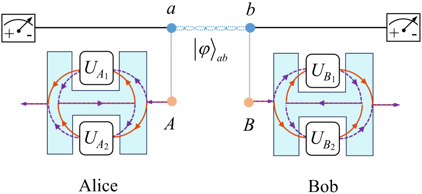
Figure 2: Schematic diagram for generating a heralded general two-qubit quantum state on two remote particles $A$ and $B$ via two quantum switches. First, a maximally entangled state $|\varphi\rangle_{ab}$ is shared with Alice and Bob. Qubits $a$ and $b$ act as the control qubits, which conditionally manipulate the operation order on target qubits $A$ and $B$ via their individual quantum switches, respectively. When the control qubit $a$ ($b$) is in the state $|0\rangle_{a}$ ($|0\rangle_{b}$), the operation order of single-qubit gates is that $U_{A_{1}}$ ($U_{B_{1}}$) is before $U_{A_{2}}$ ($U_{B_{2}}$), i.e., $U_{A_{2}}U_{A_{1}}$ ($U_{B_{2}}U_{B_{1}}$), denoted by the purple circuit. When the control qubit $a$ ($b$) is in the state $|1\rangle_{a}$ ($|1\rangle_{b}$), the operation order of single-qubit gates is that $U_{A_{2}}$ ($U_{B_{2}}$) is before $U_{A_{1}}$ ($U_{B_{1}}$), i.e., $U_{A_{1}}U_{A_{2}}$ ($U_{B_{1}}U_{B_{2}}$), denoted by the red circuit. Lastly, the qubits $a$ and $b$ are measured in the basis $\{|\pm\rangle\}$, the target state of particles $AB$ will automatically become a MES, PES, or SS, by appropriately employing the single-qubit gates $U_{A_{1}}$, $U_{A_{2}}$, $U_{B_{1}}$, and $U_{B_{2}}$.

Alice and Bob measure the two control qubits $a$ and $b$ in the basis $\{|\pm\rangle\}$, respectively. If the measurement results are $|+\rangle_{a}|+\rangle_{b}$ or $|-\rangle_{a}|-\rangle_{b}$, the state $|\Phi_{1}^{\prime}\rangle$ will collapse to a normalized state

$$\begin{split}|\Phi_{2}\rangle=&\;\frac{1}{\sqrt{2}}[(U_{A_{2}}U_{A_{1}})\otimes(U_{B_{2}}U_{B_{1}})\\ &+(U_{A_{1}}U_{A_{2}})\otimes(U_{B_{1}}U_{B_{2}})]|\psi\rangle_{A}|\psi\rangle_{B},\end{split}$$ (9)

with a success probability of $\frac{1}{2}$. If the measurement results are $|+\rangle_{a}|-\rangle_{b}$ or $|-\rangle_{a}|+\rangle_{b}$, the state $|\Phi_{1}^{\prime}\rangle$ will collapse to a normalized state

$$\begin{split}|\Phi_{2}^{\prime}\rangle=&\;\frac{1}{\sqrt{2}}[(U_{A_{2}}U_{A_{1}})\otimes(U_{B_{2}}U_{B_{1}})\\ &-(U_{A_{1}}U_{A_{2}})\otimes(U_{B_{1}}U_{B_{2}})]|\psi\rangle_{A}|\psi\rangle_{B},\end{split}$$ (10)

with a success probability of $\frac{1}{2}$.

More generally, in the above approach, operations $\frac{1}{\sqrt{2}}[(U_{A_{2}}U_{A_{1}})\otimes(U_{B_{2}}U_{B_{1}})\pm(U_{A_{1}}U_{A_{2}})\otimes(U_{B_{1}}U_{B_{2}})]$ are applied to transform the initial product state $|\psi\rangle_{A}\otimes|\psi\rangle_{B}$ into a MES, PES, or EE. To achieve this aim, we introduce the following single-qubit gates $U_{A_{1}},U_{A_{2}},U_{B_{1}}$, and $U_{B_{2}}$:

$$\begin{split}&U_{A_{2}}=X=\left(\begin{array}[]{cc}0&1\\ 1&0\\ \end{array}\right),\\ &U_{B_{2}}=X=\left(\begin{array}[]{cc}0&1\\ 1&0\\ \end{array}\right),\\ &U_{A_{1}}=R_{y}(2\theta)=\left(\begin{array}[]{cc}\cos\theta&-\sin\theta\\ \sin\theta&\cos\theta\\ \end{array}\right),\\ &U_{B_{1}}=R_{y}(2\theta)=\left(\begin{array}[]{cc}\cos\theta&-\sin\theta\\ \sin\theta&\cos\theta\\ \end{array}\right).\end{split}$$ (11)

Here $\theta\in[0,2\pi]$. Substituting Eq. (LABEL:eq11) into Eq. (9) and Eq. (10), the states $|\Phi_{2}\rangle$ and $|\Phi_{2}^{\prime}\rangle$ can be rewritten as

$$\begin{split}|\Phi_{2}\rangle=&\;\sqrt{2}[(\sqrt{(1-\alpha_{A})(1-\alpha_{B})}\cos^{2}\theta\\ &+\sqrt{\alpha_{A}\alpha_{B}}\sin^{2}\theta)|0\rangle_{A}|0\rangle_{B}\\ &+(\sqrt{(1-\alpha_{A})\alpha_{B}}\cos^{2}\theta\\ &-\sqrt{\alpha_{A}(1-\alpha_{B})}\sin^{2}\theta)|0\rangle_{A}|1\rangle_{B}\\ &+(\sqrt{\alpha_{A}(1-\alpha_{B})}\cos^{2}\theta\\ &-\sqrt{(1-\alpha_{A})\alpha_{B}}\sin^{2}\theta)|1\rangle_{A}|0\rangle_{B}\\ &+(\sqrt{\alpha_{A}\alpha_{B}}\cos^{2}\theta\\ &+\sqrt{(1-\alpha_{A})(1-\alpha_{B})}\sin^{2}\theta)|1\rangle_{A}|1\rangle_{B}].\end{split}$$ (12)

$$\begin{split}|\Phi_{2}^{\prime}\rangle=&\;\frac{1}{\sqrt{2}}\sin 2\theta[(\sqrt{\alpha_{A}(1-\alpha_{B})}+\sqrt{(1-\alpha_{A})\alpha_{B}})\\ &\times(|0\rangle_{A}|0\rangle_{B}-|1\rangle_{A}|1\rangle_{B})+(\sqrt{\alpha_{A}\alpha_{B}}\\ &-\sqrt{(1-\alpha_{A})(1-\alpha_{B})})(|0\rangle_{A}|1\rangle_{B}+|1\rangle_{A}|0\rangle_{B})].\end{split}$$ (13)

As shown in Table 1, based on Eqs. (12)-(13) and the specific choice of parameters, the measurement results, output states, and the types of output states can be classified as follows:

(i) If the measurement results are $|+\rangle_{a}|+\rangle_{b}$ or $|-\rangle_{a}|-\rangle_{b}$, the output state will be $|\Phi_{2}\rangle$. (a) When $\theta=\frac{\pi}{4}$, $\frac{3\pi}{4}$, $\frac{5\pi}{4}$, $\frac{7\pi}{4}$ with $\alpha_{A}=\alpha_{B}=\frac{1}{2}$ or 0, or 1, the state $|\Phi_{2}\rangle$ will become a MES, i.e., $|\Phi_{2}\rangle=|\Phi^{+}\rangle=\frac{1}{\sqrt{2}}(|0\rangle_{A}|0\rangle_{B}+|1\rangle_{A}|1\rangle_{B})$. (b) When $\theta=\frac{\pi}{4}$, $\frac{3\pi}{4}$, $\frac{5\pi}{4}$, $\frac{7\pi}{4}$ with $\alpha_{A}=0$ and $\alpha_{B}=1$, the state $|\Phi_{2}\rangle$ will become a MES, i.e., $|\Phi_{2}\rangle=|\Psi^{-}\rangle=\frac{1}{\sqrt{2}}(|0\rangle_{A}|1\rangle_{B}-|1\rangle_{A}|0\rangle_{B})$. (c) When $\theta=\frac{\pi}{4}$, $\frac{3\pi}{4}$, $\frac{5\pi}{4}$, $\frac{7\pi}{4}$ with $\alpha_{A}=1$ and $\alpha_{B}=0$, the state $|\Phi_{2}\rangle$ will become a MES, i.e., $|\Phi_{2}\rangle=-|\Psi^{-}\rangle$.

(ii) If the measurement results are $|+\rangle_{a}|-\rangle_{b}$ or $|-\rangle_{a}|+\rangle_{b}$, the output state will be $|\Phi_{2}^{\prime}\rangle$. (a) When $\theta=\frac{\pi}{4}$, $\frac{3\pi}{4}$, $\frac{5\pi}{4}$, $\frac{7\pi}{4}$ with $\alpha_{A}=\alpha_{B}=\frac{1}{2}$ (or $\alpha_{A}=0$, $\alpha_{B}=1$, or $\alpha_{A}=1$, $\alpha_{B}=0$), the state $|\Phi_{2}^{\prime}\rangle$ will become a MES, i.e., $|\Phi_{2}^{\prime}\rangle=\pm|\Phi^{-}\rangle=\pm\frac{1}{\sqrt{2}}(|0\rangle_{A}|0\rangle_{B}-|1\rangle_{A}|1\rangle_{B})$. (b) When $\theta=\frac{\pi}{4}$, $\frac{3\pi}{4}$, $\frac{5\pi}{4}$, $\frac{7\pi}{4}$ with $\alpha_{A}=\alpha_{B}=0$ (or $\alpha_{A}=\alpha_{B}=1$), the state $|\Phi_{2}^{\prime}\rangle$ will become a MES, i.e., $|\Phi_{2}^{\prime}\rangle=\pm|\Psi^{+}\rangle=\pm\frac{1}{\sqrt{2}}(|0\rangle_{A}|1\rangle_{B}+|1\rangle_{A}|0\rangle_{B})$.

(iii) If $\theta=0$, $\pi$, $2\pi$ or $\theta=\frac{\pi}{2}$, $\frac{3\pi}{2}$, no matter what the values of $\alpha_{A}$ and $\alpha_{B}$ are taken, no entanglement state can be obtained. Specifically, (a) when $\theta=0$, $\pi$, $2\pi$, the state $|\Phi_{2}\rangle$ will become a SS, i.e., $|\Phi_{2}\rangle=|\Phi^{xx}\rangle=\sigma_{x}^{A}\sigma_{x}^{B}(|\psi\rangle_{A}\otimes|\psi\rangle_{B})$, while $|\Phi_{2}^{\prime}\rangle$ will vanish. (b) When $\theta=\frac{\pi}{2}$, $\frac{3\pi}{2}$, the state $|\Phi_{2}\rangle$ will become a SS, i.e., $|\Phi_{2}\rangle=|\Phi^{zz}\rangle=\sigma_{z}^{A}\sigma_{z}^{B}(|\psi\rangle_{A}\otimes|\psi\rangle_{B})$, while $|\Phi_{2}^{\prime}\rangle$ will vanish. Here $\sigma_{x}^{A}$ ($\sigma_{x}^{B}$) and $\sigma_{z}^{A}$ ($\sigma_{z}^{B}$) are the Pauli $X$ and Pauli $Z$ gates acting on qubit $A$ ($B$).

(iv) For all other cases, the output states $|\Phi_{2}\rangle$ and $|\Phi_{2}^{\prime}\rangle$ both are PES.

Therefore, the protocol illustrated in Fig. 2 deterministically generates a two-qubit MES on two long-distance quibts $A$ and $B$. The success of the protocol is heralded by the measurement outcomes of qubits $a$ and $b$. If we wish to obtain the same output states, two-bit classical communication between Alice and Bob, along with some feed-forward operations on qubits $A$ and $B$, will be required.

Table 1: The relations between the angle $\theta$ described in Eq. (LABEL:eq11), the measurement results of qubits $a$ and $b$, and the output states $|\Phi_{2}\rangle$ and $|\Phi_{2}^{\prime}\rangle$. $\theta\in[0,2\pi]$ and $n=1,2,3,4$. $|\Phi^{\pm}\rangle=\frac{1}{\sqrt{2}}(|0\rangle_{A}|0\rangle_{B}\pm|1\rangle_{A}|1\rangle_{B})$, $|\Psi^{\pm}\rangle=\frac{1}{\sqrt{2}}(|0\rangle_{A}|1\rangle_{B}\pm|1\rangle_{A}|0\rangle_{B})$, $|\Phi^{xx}\rangle=\sigma_{x}^{A}\sigma_{x}^{B}(|\psi\rangle_{A}\otimes|\psi\rangle_{B})$, and $|\Phi^{zz}\rangle=\sigma_{z}^{A}\sigma_{z}^{B}(|\psi\rangle_{A}\otimes|\psi\rangle_{B})$, where $\sigma_{x}^{A}$ ($\sigma_{x}^{B}$) and $\sigma_{z}^{A}$ ($\sigma_{z}^{B}$) are the Pauli $X$ and Pauli $Z$ gates acting on qubit $A$ ($B$).

$\theta$	$\alpha_{A}$	$\alpha_{B}$	Measured result	Output state	Type
$\frac{(2n-1)\pi}{4}$	$\frac{1}{2}$	$\frac{1}{2}$	$|+\rangle_{a}|+\rangle_{b},\,|-\rangle_{a}|-\rangle_{b}$ $|+\rangle_{a}|-\rangle_{b},\,|-\rangle_{a}|+\rangle_{b}$	$|\Phi_{2}\rangle=|\Phi^{+}\rangle$ $|\Phi_{2}^{\prime}\rangle=\pm|\Phi^{-}\rangle$	MES
$\frac{(2n-1)\pi}{4}$	0	0	$|+\rangle_{a}|+\rangle_{b},\,|-\rangle_{a}|-\rangle_{b}$ $|+\rangle_{a}|-\rangle_{b},\,|-\rangle_{a}|+\rangle_{b}$	$|\Phi_{2}\rangle=|\Phi^{+}\rangle$ $|\Phi_{2}^{\prime}\rangle=\pm|\Psi^{+}\rangle$	MES
$\frac{(2n-1)\pi}{4}$	1	1	$|+\rangle_{a}|+\rangle_{b},\,|-\rangle_{a}|-\rangle_{b}$ $|+\rangle_{a}|-\rangle_{b},\,|-\rangle_{a}|+\rangle_{b}$	$|\Phi_{2}\rangle=|\Phi^{+}\rangle$ $|\Phi_{2}^{\prime}\rangle=\pm|\Psi^{+}\rangle$	MES
$\frac{(2n-1)\pi}{4}$	0	1	$|+\rangle_{a}|+\rangle_{b},\,|-\rangle_{a}|-\rangle_{b}$ $|+\rangle_{a}|-\rangle_{b},\,|-\rangle_{a}|+\rangle_{b}$	$|\Phi_{2}\rangle=|\Psi^{-}\rangle$ $|\Phi_{2}^{\prime}\rangle=\pm|\Phi^{-}\rangle$	MES
$\frac{(2n-1)\pi}{4}$	1	0	$|+\rangle_{a}|+\rangle_{b},\,|-\rangle_{a}|-\rangle_{b}$ $|+\rangle_{a}|-\rangle_{b},\,|-\rangle_{a}|+\rangle_{b}$	$|\Phi_{2}\rangle=-|\Psi^{-}\rangle$ $|\Phi_{2}^{\prime}\rangle=\pm|\Phi^{-}\rangle$	MES
$0,\pi,2\pi$	Any	Any	$|+\rangle_{a}|+\rangle_{b},\,|-\rangle_{a}|-\rangle_{b}$ $|+\rangle_{a}|-\rangle_{b},\,|-\rangle_{a}|+\rangle_{b}$	$|\Phi_{2}\rangle=|\Phi^{xx}\rangle$ $|\Phi_{2}^{\prime}\rangle=\textbf{0}$	SS 0 state
$\frac{\pi}{2},\frac{3\pi}{2}$	Any	Any	$|+\rangle_{a}|+\rangle_{b},\,|-\rangle_{a}|-\rangle_{b}$ $|+\rangle_{a}|-\rangle_{b},\,|-\rangle_{a}|+\rangle_{b}$	$|\Phi_{2}\rangle=|\Phi^{zz}\rangle$ $|\Phi_{2}^{\prime}\rangle=\textbf{0}$	SS 0 state

II.2 Entangled state generation among three long-distance qubits

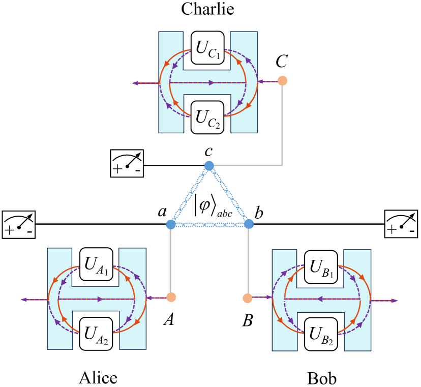
Figure 3: Schematic diagram for generating a heralded general three-qubit quantum state on three remote particles $A$, $B$, and $C$ via three quantum switches. First, a maximally entangled state $|\varphi\rangle_{abc}$ is shared with Alice, Bob, and Charlie. Qubits $a$, $b$, and $c$ act as the control qubit that manipulate the operation order on target qubits $A$, $B$, and $C$ via their individual quantum switches, respectively. When the control qubit $a$ is in the state $|0\rangle_{a}$, the operation order of single-qubit gate is that $U_{A_{1}}$ is before $U_{A_{2}}$, i.e., $U_{A_{2}}U_{A_{1}}$, denoted by the purple circuit. When the control qubit $a$ is in the state $|1\rangle_{a}$, the operation order of single-qubit gate is that $U_{A_{2}}$ is before $U_{A_{1}}$, i.e., $U_{A_{1}}U_{A_{2}}$, denoted by the red circuit. Bob and Charlie come to the same conclusion. Finally, qubits $a$, $b$, and $c$ are measured in the basis $\{|\pm\rangle\}$, the state $ABC$ will become a MES, PES, or SS, by appropriately introducing the single-qubit gates $U_{A_{1}}$, $U_{A_{2}}$, $U_{B_{1}}$, $U_{B_{2}}$, $U_{C_{1}}$, and $U_{C_{2}}$.

Suppose that three parties Alice, Bob, and Charlie possess particles $A$, $B$, and $C$, respectively. These particles are initially prepared as

$$|\psi\rangle_{A}=\sqrt{\alpha_{A}}|0\rangle_{A}+\sqrt{1-\alpha_{A}}|1\rangle_{A},$$ (14)

$$|\psi\rangle_{B}=\sqrt{\alpha_{B}}|0\rangle_{B}+\sqrt{1-\alpha_{B}}|1\rangle_{B},$$ (15)

$$|\psi\rangle_{C}=\sqrt{\alpha_{C}}|0\rangle_{C}+\sqrt{1-\alpha_{C}}|1\rangle_{C}.$$ (16)

The objective of Alice, Bob, and Charlie is to transform the given separable state $|\psi\rangle_{A}\otimes|\psi\rangle_{B}\otimes|\psi\rangle_{C}$ into a general three-qubit state.

As shown in Fig. 3, we propose a heralded scheme for the deterministic implementation of a general long-distance three-qubit state. The detailed procedure of our protocol is outlined step by step below.

Step 1: A three-qubit maximally entangled state

$$|\varphi\rangle_{abc}=\frac{1}{\sqrt{2}}(|0\rangle_{a}|0\rangle_{b}|0\rangle_{c}+|1\rangle_{a}|1\rangle_{b}|1\rangle_{c}),$$ (17)

is shared with Alice, Bob, and Charlie. Here particles $a$, $b$, and $c$ are held by Alice, Bob, and Charlie, respectively. The state of the whole system is given by

$$\begin{split}|\Psi\rangle_{0}=&\;|\varphi\rangle_{abc}\otimes|\psi\rangle_{A}\otimes|\psi\rangle_{B}\otimes|\psi\rangle_{C}\\ =&\;\frac{1}{\sqrt{2}}(|0\rangle_{a}|0\rangle_{b}|0\rangle_{c}+|1\rangle_{a}|1\rangle_{b}|1\rangle_{c})\\ &\otimes|\psi\rangle_{A}\otimes|\psi\rangle_{B}\otimes|\psi\rangle_{C}.\end{split}$$ (18)

Table 2: The correspondence between the values of rotation angle $\theta$, coefficients $\alpha_{A}$, $\alpha_{B}$, $\alpha_{C}$, measured results on qubits $a$, $b$, $c$, the final output states on qubits $A$, $B$, $C$, and the state type of output states. $|\Phi_{3}^{\pm}\rangle=\frac{1}{\sqrt{2}}(|0\rangle_{A}|0\rangle_{B}|0\rangle_{C}\pm|1\rangle_{A}|1\rangle_{B}|1\rangle_{C})$, $|\Phi^{xxx}\rangle=\sigma_{x}^{A}\sigma_{x}^{B}\sigma_{x}^{C}(|\psi\rangle_{A}\otimes|\psi\rangle_{B}\otimes|\psi\rangle_{C})$, and $|\Phi^{zzz}\rangle=\sigma_{z}^{A}\sigma_{z}^{B}\sigma_{z}^{C}(|\psi\rangle_{A}\otimes|\psi\rangle_{B}\otimes|\psi\rangle_{C})$.

$\theta$	$\alpha_{A}$	$\alpha_{B}$	$\alpha_{C}$	Measured result	Output state	State type
$\frac{(2n-1)\pi}{4}$	$\frac{1}{2}$	$\frac{1}{2}$	$\frac{1}{2}$	$|+\rangle_{a}|+\rangle_{b}|+\rangle_{c},\,|+\rangle_{a}|-\rangle_{b}|-\rangle_{c},\,|-\rangle_{a}|+\rangle_{b}|-\rangle_{c},\,|-\rangle_{a}|-\rangle_{b}|+\rangle_{c}$ $|+\rangle_{a}|+\rangle_{b}|-\rangle_{c},\,|+\rangle_{a}|-\rangle_{b}|+\rangle_{c},\,|-\rangle_{a}|+\rangle_{b}|+\rangle_{c},\,|-\rangle_{a}|-\rangle_{b}|-\rangle_{c}$	$|\Psi_{2}\rangle=|\Phi^{+}_{3}\rangle$ $|\Psi_{2}^{\prime}\rangle=|\Phi_{3}^{-}\rangle$	MES
$0,\pi,2\pi$	Any	Any	Any	$|+\rangle_{a}|+\rangle_{b}|+\rangle_{c},\,|+\rangle_{a}|-\rangle_{b}|-\rangle_{c},\,|-\rangle_{a}|+\rangle_{b}|-\rangle_{c},\,|-\rangle_{a}|-\rangle_{b}|+\rangle_{c}$ $|+\rangle_{a}|+\rangle_{b}|-\rangle_{c},\,|+\rangle_{a}|-\rangle_{b}|+\rangle_{c},\,|-\rangle_{a}|+\rangle_{b}|+\rangle_{c},\,|-\rangle_{a}|-\rangle_{b}|-\rangle_{c}$	$|\Psi_{2}\rangle=|\Phi^{xxx}\rangle$ $|\Psi_{2}^{\prime}\rangle=\textbf{0}$	SS 0 state
$\frac{\pi}{2},\frac{3\pi}{2}$	Any	Any	Any	$|+\rangle_{a}|+\rangle_{b}|+\rangle_{c},\,|+\rangle_{a}|-\rangle_{b}|-\rangle_{c},\,|-\rangle_{a}|+\rangle_{b}|-\rangle_{c},\,|-\rangle_{a}|-\rangle_{b}|+\rangle_{c}$ $|+\rangle_{a}|+\rangle_{b}|-\rangle_{c},\,|+\rangle_{a}|-\rangle_{b}|+\rangle_{c},\,|-\rangle_{a}|+\rangle_{b}|+\rangle_{c},\,|-\rangle_{a}|-\rangle_{b}|-\rangle_{c}$	$|\Psi_{2}\rangle=\textbf{0}$ $|\Psi_{2}^{\prime}\rangle=|\Phi^{zzz}\rangle$	0 state SS

Step 2: A similar arrangement as that made in Sec. II.1. Qubits $a$, $b$ and $c$ act as the control qubits to govern the order of single-qubit gates on qubits $A$, $B$, and $C$ by resorting to their individual quantum switches. Here each quantum switch non-trivially performs the gate operations in the order $U_{i_{2}}U_{i_{1}}$ ($i=A$, $B$, and $C$) when the control qubit is in the state $|0\rangle$, while the gate operations are performed in the order $U_{i_{1}}U_{i_{2}}$ ($i=A$, $B$, and $C$) when the control qubit is in the state $|1\rangle$. Thus, three quantum switches change the initial state $|\Psi\rangle_{0}$ into

$$\begin{split}|\Psi_{1}\rangle=&\;\frac{1}{\sqrt{2}}[|0\rangle_{a}(U_{A_{2}}U_{A_{1}}|\psi\rangle_{A})\otimes|0\rangle_{b}(U_{B_{2}}U_{B_{1}}|\psi\rangle_{B})\\ &\otimes|0\rangle_{c}(U_{C_{2}}U_{C_{1}}|\psi\rangle_{C})+|1\rangle_{a}(U_{A_{1}}U_{A_{2}}|\psi\rangle_{A})\\ &\otimes|1\rangle_{b}(U_{B_{1}}U_{B_{2}}|\psi\rangle_{B})\otimes|1\rangle_{c}(U_{C_{1}}U_{C_{2}}|\psi\rangle_{C})].\end{split}$$ (19)

Step 3: Alice, Bob, and Charlie measure the control qubits $a$, $b$, and $c$ in the basis $\{|\pm\rangle\}$, respectively. If the measured results are $|+\rangle_{a}|+\rangle_{b}|+\rangle_{c}$, $|+\rangle_{a}|-\rangle_{b}|-\rangle_{c}$, $|-\rangle_{a}|+\rangle_{b}|-\rangle_{c}$, or $|-\rangle_{a}|-\rangle_{b}|+\rangle_{c}$, the state $|\Psi_{1}\rangle$ will collapse to a normalized state

$$\begin{split}|\Psi_{2}\rangle=&\;\frac{1}{\sqrt{2}}[(U_{A_{2}}U_{A_{1}})\otimes(U_{B_{2}}U_{B_{1}})\otimes(U_{C_{2}}U_{C_{1}})\\ &+(U_{A_{1}}U_{A_{2}})\otimes(U_{B_{1}}U_{B_{2}})\otimes(U_{C_{1}}U_{C_{2}})](|\psi\rangle_{A}\\ &\otimes|\psi\rangle_{B}\otimes|\psi\rangle_{C}),\end{split}$$ (20)

with a success probability of $\frac{1}{2}$. If the measured results are $|+\rangle_{a}|+\rangle_{b}|-\rangle_{c}$, $|+\rangle_{a}|-\rangle_{b}|+\rangle_{c}$, $|-\rangle_{a}|+\rangle_{b}|+\rangle_{c}$, or $|-\rangle_{a}|-\rangle_{b}|-\rangle_{c}$, then the state $|\Psi_{1}\rangle$ will collapse into

$$\begin{split}|\Psi_{2}^{\prime}\rangle=&\;\frac{1}{\sqrt{2}}[(U_{A_{2}}U_{A_{1}})\otimes(U_{B_{2}}U_{B_{1}})\otimes(U_{C_{2}}U_{C_{1}})\\ &-(U_{A_{1}}U_{A_{2}})\otimes(U_{B_{1}}U_{B_{2}})\otimes(U_{C_{1}}U_{C_{2}})]\\ &\otimes(|\psi\rangle_{A}\otimes|\psi\rangle_{B}\otimes|\psi\rangle_{C}),\end{split}$$ (21)

with a probability of $\frac{1}{2}$. To obtain a general quantum state of remote qubits $A$, $B$, and $C$, we introduce

$$\begin{split}&U_{A_{2}}=U_{B_{2}}=U_{C_{2}}=X,\\ &U_{A_{1}}=U_{B_{1}}=U_{C_{1}}=R_{y}(2\theta).\end{split}$$ (22)

Then, $|\Psi_{2}\rangle$ and $|\Psi_{2}^{\prime}\rangle$ can be reexpressed as:

$$\begin{split}|\Psi_{2}\rangle=&\;\frac{1}{\sqrt{2}}[(\alpha_{2}\sin\theta\sin 2\theta+\alpha_{3}\sin\theta\sin 2\theta\\ &+\alpha_{5}\sin\theta\sin 2\theta+2\alpha_{8}\cos^{3}\theta)|0\rangle_{A}|0\rangle_{B}|0\rangle_{C}\\ &+(\alpha_{1}\sin\theta\sin 2\theta-\alpha_{4}\sin\theta\sin 2\theta\\ &-\alpha_{6}\sin\theta\sin 2\theta+2\alpha_{7}\cos^{3}\theta)|0\rangle_{A}|0\rangle_{B}|1\rangle_{C}\\ &+(\alpha_{1}\sin\theta\sin 2\theta-\alpha_{4}\sin\theta\sin 2\theta\\ &+2\alpha_{6}\cos^{3}\theta-\alpha_{7}\sin\theta\sin 2\theta)|0\rangle_{A}|1\rangle_{B}|0\rangle_{C}\\ &-(\alpha_{2}\sin\theta\sin 2\theta+\alpha_{3}\sin\theta\sin 2\theta\\ &-2\alpha_{5}\cos^{3}\theta-\alpha_{8}\sin\theta\sin 2\theta)|0\rangle_{A}|1\rangle_{B}|1\rangle_{C}\\ &+(\alpha_{1}\sin\theta\sin 2\theta+2\alpha_{4}\cos^{3}\theta\\ &-\alpha_{6}\sin\theta\sin 2\theta-\alpha_{7}\sin\theta\sin 2\theta)|1\rangle_{A}|0\rangle_{B}|0\rangle_{C}\\ &-(\alpha_{2}\sin\theta\sin 2\theta-2\alpha_{3}\cos^{3}\theta\\ &+\alpha_{5}\sin\theta\sin 2\theta-\alpha_{8}\sin\theta\sin 2\theta)|1\rangle_{A}|0\rangle_{B}|1\rangle_{C}\\ &+(2\alpha_{2}\cos^{3}\theta-\alpha_{3}\sin\theta\sin 2\theta\\ &-\alpha_{5}\sin\theta\sin 2\theta+\alpha_{8}\sin\theta\sin 2\theta)|1\rangle_{A}|1\rangle_{B}|0\rangle_{C}\\ &+(2\alpha_{1}\cos^{3}\theta+\alpha_{4}\sin\theta\sin 2\theta\\ &+\alpha_{6}\sin\theta\sin 2\theta+\alpha_{7}\sin\theta\sin 2\theta)|1\rangle_{A}|1\rangle_{B}|1\rangle_{C}].\end{split}$$ (23)

$$\begin{split}|\Psi_{2}^{\prime}\rangle=&\;\frac{1}{\sqrt{2}}[(2\alpha_{1}\sin^{3}\theta+\alpha_{4}\cos\theta\sin 2\theta\\ &+\alpha_{6}\cos\theta\sin 2\theta+\alpha_{7}\cos\theta\sin 2\theta)|0\rangle_{A}|0\rangle_{B}|0\rangle_{C}\\ &-(2\alpha_{2}\sin^{3}\theta-\alpha_{3}\cos\theta\sin 2\theta\\ &-\alpha_{5}\cos\theta\sin 2\theta+\alpha_{8}\cos\theta\sin 2\theta)|0\rangle_{A}|0\rangle_{B}|1\rangle_{C}\\ &+(\alpha_{2}\cos\theta\sin 2\theta-2\alpha_{3}\sin^{3}\theta\\ &+\alpha_{5}\cos\theta\sin 2\theta-\alpha_{8}\cos\theta\sin 2\theta)|0\rangle_{A}|1\rangle_{B}|0\rangle_{C}\\ &+(\alpha_{1}\cos\theta\sin 2\theta-\alpha_{6}\cos\theta\sin 2\theta\\ &+2\alpha_{4}\sin^{3}\theta-\alpha_{7}\cos\theta\sin 2\theta)|0\rangle_{A}|1\rangle_{B}|1\rangle_{C}\\ &+(\alpha_{2}\cos\theta\sin 2\theta+\alpha_{3}\cos\theta\sin 2\theta\\ &-2\alpha_{5}\sin^{3}\theta-\alpha_{8}\cos\theta\sin 2\theta)|1\rangle_{A}|0\rangle_{B}|0\rangle_{C}\\ &+(\alpha_{1}\cos\theta\sin 2\theta-\alpha_{4}\cos\theta\sin 2\theta\\ &+2\alpha_{6}\sin^{3}\theta-\alpha_{7}\cos\theta\sin 2\theta)|1\rangle_{A}|0\rangle_{B}|1\rangle_{C}\\ &+(\alpha_{1}\cos\theta\sin 2\theta-\alpha_{4}\cos\theta\sin 2\theta\\ &-\alpha_{6}\cos\theta\sin 2\theta+2\alpha_{7}\sin^{3}\theta)|1\rangle_{A}|1\rangle_{B}|0\rangle_{C}\\ &-(\alpha_{2}\cos\theta\sin 2\theta+\alpha_{3}\cos\theta\sin 2\theta\\ &+\alpha_{5}\cos\theta\sin 2\theta+2\alpha_{8}\sin^{3}\theta)|1\rangle_{A}|1\rangle_{B}|1\rangle_{C}].\end{split}$$ (24)

For convenience, we here denote the coefficients as

$$\begin{split}\alpha_{1}=&\;\sqrt{\alpha_{A}\alpha_{B}\alpha_{C}},\\ \alpha_{2}=&\;\sqrt{\alpha_{A}\alpha_{B}(1-\alpha_{C})},\\ \alpha_{3}=&\;\sqrt{\alpha_{A}(1-\alpha_{B})\alpha_{C}},\\ \alpha_{4}=&\;\sqrt{\alpha_{A}(1-\alpha_{B})(1-\alpha_{C})},\\ \alpha_{5}=&\;\sqrt{(1-\alpha_{A})\alpha_{B}\alpha_{C}},\\ \alpha_{6}=&\;\sqrt{(1-\alpha_{A})\alpha_{B}(1-\alpha_{C})},\\ \alpha_{7}=&\;\sqrt{(1-\alpha_{A})(1-\alpha_{B})\alpha_{C}},\\ \alpha_{8}=&\;\sqrt{(1-\alpha_{A})(1-\alpha_{B})(1-\alpha_{C})}.\end{split}$$ (25)

Table 2 presents the relations between the values of parameters, measured results, the final output states, and state type of output states on qubits $A$, $B$, and $C$. As shown in Tab. 2, the output states can be classified into four groups: MES, SS, vanished state, and PES.

(i) In the MES group, when the angle $\theta=\frac{\pi}{4}$, $\frac{3\pi}{4}$, $\frac{5\pi}{4}$, $\frac{7\pi}{4}$ with $\alpha_{A}=\alpha_{B}=\alpha_{C}=\frac{1}{2}$ are taken, the MESs $|\Psi_{2}\rangle=\frac{1}{\sqrt{2}}(|0\rangle_{A}|0\rangle_{B}|0\rangle_{C}+|1\rangle_{A}|1\rangle_{B}|1\rangle_{C})$ and $|\Psi_{2}^{\prime}\rangle=\frac{1}{\sqrt{2}}(|0\rangle_{A}|0\rangle_{B}|0\rangle_{C}-|1\rangle_{A}|1\rangle_{B}|1\rangle_{C})$ are obtained.

(ii) In the SS group, when $\theta=0$, $\pi$, or $2\pi$, the state $|\Psi_{2}\rangle$ becomes a coefficient-independent SS $|\Psi_{2}\rangle=|\Phi^{xxx}\rangle=\sigma_{x}^{A}\sigma_{x}^{B}\sigma_{x}^{C}(|\psi\rangle_{A}\otimes|\psi\rangle_{B}\otimes|\psi\rangle_{C})$. Similarly, when $\theta=\frac{\pi}{2}$ or $\frac{3\pi}{2}$, the state $|\Psi_{2}^{\prime}\rangle$ becomes a coefficient-independent SS $|\Psi_{2}^{\prime}\rangle=|\Phi^{zzz}\rangle=\sigma_{z}^{A}\sigma_{z}^{B}\sigma_{z}^{C}(|\psi\rangle_{A}\otimes|\psi\rangle_{B}\otimes|\psi\rangle_{C})$.

(iii) In the vanished state group, when $\theta=0$, $\pi$, or $2\pi$, the state $|\Psi_{2}^{\prime}\rangle=\textbf{0}$ will be vanished for all possible coefficients $\alpha_{A},\alpha_{B}$, and $\alpha_{C}$. Similarly, when $\theta=\frac{\pi}{2}$ or $\frac{3\pi}{2}$, the state $|\Psi_{2}\rangle=\textbf{0}$ will be vanished for all possible coefficients $\alpha_{A},\alpha_{B}$, and $\alpha_{C}$.

(iv) In the PES group, for all other cases, the output states $|\Psi_{2}\rangle$ and $|\Psi_{2}^{\prime}\rangle$ will both be PESs.

II.3 Entangled state generation among $N$ separable long-distance qubits

As shown in Fig. 4, the method can be generalized to generate a heralded $N$-qubit entangled state on $N$ separable long-distance qubits by using $N$ quantum switches and a prior shared $n$-qubit Greenberger-Horne-Zeilinger (GHZ) state $|\varphi\rangle_{ab\ldots n}=\frac{1}{\sqrt{2}}(|0\rangle^{\otimes n}+|1\rangle^{\otimes n})_{ab\ldots n}$ among $N$ parties. Each party possesses qubits $i$ and $I$ ($i=a,\ldots,n$ and $I=A,\ldots,N$), where qubit $i$ acts as a control qubit and qubit $I$ acts as a target qubit. In each quantum switch, when control qubit is in the state $|0\rangle_{i}$ or $|1\rangle_{i}$, the different operation orders $U_{I_{2}}U_{I_{1}}$ or $U_{I_{1}}U_{I_{2}}$ are applied to qubit $I$. Finally, all control qubits are measured in the basis $\{|\pm\rangle\}$, and then the state of the whole system can collapse into an entangled state by adjusting the coefficients of the initial states and rotation angle $\theta$ of the single-qubit gates $U_{I_{1}}$. Here all single-qubit gates are defined as $U_{I_{1}}=R_{y}(2\theta)$ and $U_{I_{2}}=X$.

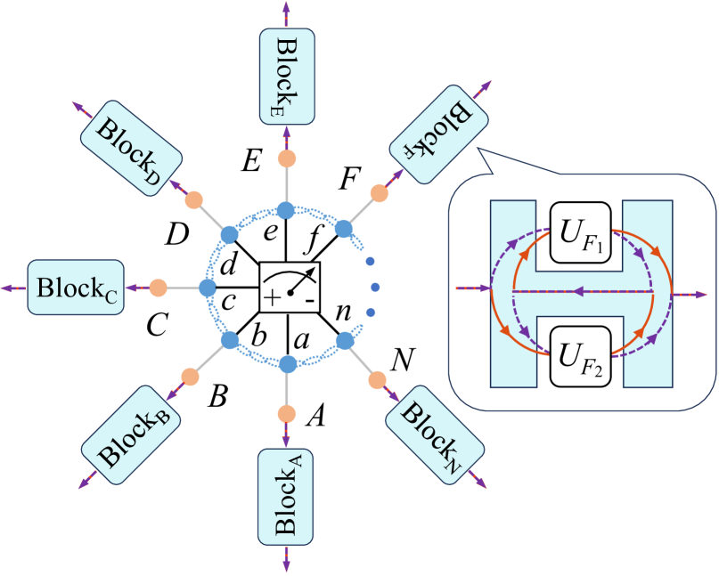
Figure 4: Schematic diagram of a scheme designed to generate a heralded $N$-qubit entangled state on $N$ remote separable qubits $A$ to $N$ via $N$ quantum switches. Here each “Block” represents a quantum switch. First, a maximally entangled state $|\varphi\rangle_{ab\ldots n}=\frac{1}{\sqrt{2}}(|0\rangle^{\otimes n}+|1\rangle^{\otimes n})_{ab\ldots n}$ is shared among $N$ parties. This shared state acts as a control qubit to conditionally manipulate the operation order of single-qubit gates by using a quantum switch held by each party. Finally, when the control qubits are measured, the state of the system can be projected into an entangled state on qubits $A$ to $N$.

III Optical realization of entangled state generation on separable long-distance qubits

The generation of entangled states on long-distance qubits can be realized via hybrid encoding in an optical system. Figure 5 illustrates an optical architecture for generating an entangled state acting on two long-distance separable polarization qubits. In this setup, the optical quantum switch is implemented with the path DoF of single photons as the control qubit, and it conditionally manipulates the order of the “target” single-qubit polarization gates in different propagation directions Procopio et al. (2015); Guo et al. (2020); Rozema et al. (2024). Let us now present the details of the scheme, step by step.

First, a maximally entangled photon pair in the polarization state

$$|\Upsilon_{0}\rangle=\frac{1}{\sqrt{2}}(|H\rangle_{a}|H\rangle_{b}+|V\rangle_{a}|V\rangle_{b}),$$ (26)

is shared with Alice and Bob. Here $H$ and $V$ denote horizontal and vertical polarization states. In experiments, the polarization entangled state $|\Upsilon_{0}\rangle$ can be generated by a pulsed laser pumping into the $\beta-$BaB₂O₄ (BBO) crystal Kwiat et al. (1999); Zhang et al. (2021) with type-I SPDC process or through type-I SPDC in a periodically poled potassium titanyl phosphate (PPKTP) crystal Jin et al. (2014); Lee et al. (2016); Chen et al. (2020). The photons $a$ and $b$ pass through two polarizing beam splitters, PBS₁ and PBS₂. PBS transmits the $H$-component and reflects the $V$-component of photon, respectively. Hence, PBS splits the path of the photon into the path states $|0\rangle_{a}$, $|1\rangle_{a}$ $|0\rangle_{b}$, and $|1\rangle_{b}$. After photons pass through PBS₁ and PBS₂, the state of the polarization-entangled photons can be rewritten as

$$|\Upsilon_{1}\rangle=\frac{1}{\sqrt{2}}(|H\rangle|0\rangle_{a}|H\rangle|0\rangle_{b}+|V\rangle|1\rangle_{a}|V\rangle|1\rangle_{b}).$$ (27)

In order to obtain a general initial state with the same form as the state shown in Eq. (4), we arrange half-wave plate HWP₁ rotated at $\lambda_{1}^{\circ}$ in the paths $|0\rangle_{a}$ and arrange HWP₃ rotated at $(\lambda_{1}+45)^{\circ}$ in the paths $|1\rangle_{a}$ to change the $H$-photon into the state $|\phi\rangle_{A}=\cos 2\lambda_{1}|H\rangle+\sin 2\lambda_{1}|V\rangle$ and change the $V$-photon into $|\phi\rangle_{A}$. We arrange HWP₂ rotated at $\lambda_{2}^{\circ}$ in the paths $|0\rangle_{b}$ and HWP₄ rotated at $(\lambda_{2}+45)^{\circ}$ in the paths $|1\rangle_{b}$ to change the $H$-photon into the state $|\phi\rangle_{B}=\cos 2\lambda_{2}|H\rangle+\sin 2\lambda_{2}|V\rangle$ and change the $V$-photon into $|\phi\rangle_{B}$. These elements (HWP₁, HWP₂, HWP₃, and HWP₄) convert $|\Upsilon_{1}\rangle$ to

$$|\Upsilon_{2}\rangle=\frac{1}{\sqrt{2}}(|0\rangle_{a}|0\rangle_{b}+|1\rangle_{a}|1\rangle_{b})\otimes|\phi\rangle_{A}\otimes|\phi\rangle_{B}.$$ (28)

Based on Eq. (26) to Eq. (28), we can find that the polarized entangled state shown in Eq. (27) is transformed into path entangled state shown in Eq. (28). Such transformation indicates that the preparation of the initial state is completed.

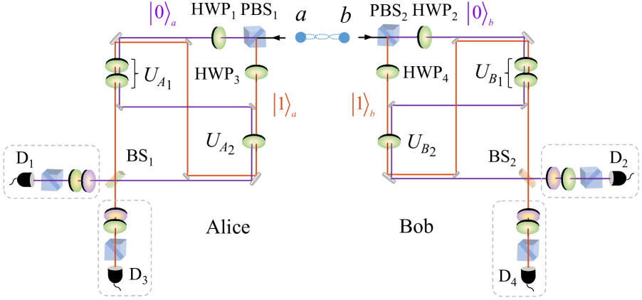
Figure 5: Schematic setup to generate optical entangled state on two separable long-distance qubits. A maximally entangled photon pair in the polarization state is shared with Alice and Bob. The paths of the photons are divided into $|0\rangle_{a}$, $|1\rangle_{a}$, $|0\rangle_{b}$, and $|1\rangle_{b}$ by two polarizing beam splitters, PBS₁ and PBS₂, because PBS transmits $H$-photon and reflects $V$-photon. The photons emitting from different paths suffer from different gate orders, i.e., $U_{A_{2}}U_{A_{1}}$ ($U_{B_{2}}U_{B_{1}}$) or $U_{A_{1}}U_{A_{2}}$ ($U_{B_{1}}U_{B_{2}}$) and then mix at beam splitters BS₁ and BS₂. Before each detection of path qubits, a polarization analyzer, consisting of a quarter-wave plate (QWP), a half-wave plate (HWP), and a PBS, is inserted to measure the polarization state in an arbitrary basis.

Second, the path states act as control qubits to manipulate the operation order of polarization gates on states $|\phi\rangle_{A}$ and $|\phi\rangle_{B}$. If the photon is in path $|0\rangle_{a}$ (or $|0\rangle_{b}$), it suffers from $U_{A_{1}}$ (or $U_{B_{1}}$) followed by $U_{A_{2}}$ (or $U_{B_{2}}$). If the photon is in path $|1\rangle_{a}$ (or $|1\rangle_{b}$), it passes through $U_{A_{2}}$ (or $U_{B_{2}}$) followed by $U_{A_{1}}$ (or $U_{B_{1}}$). The operations $U_{A_{1}}$, $U_{B_{1}}$, $U_{A_{2}}$, $U_{B_{2}}$ are the single-qubit polarization gates. For $U_{A_{2}}=U_{B_{2}}=X$ case, they can be easily realized by an HWP rotated at $45^{\circ}$. For $U_{A_{1}}=U_{B_{1}}=R_{y}(2\theta)$ case, they can be realized by an HWP rotated at $0^{\circ}$ and an HWP rotated at $\frac{\theta}{2}^{\circ}$. Then the photons from two paths $|0\rangle_{a}$ and $|1\rangle_{a}$ ($|0\rangle_{b}$ and $|1\rangle_{b}$) arrive at a balanced beam splitter BS₁ (BS₂), simultaneously. These optical elements $U_{A_{1}}$, $U_{A_{2}}$, $U_{B_{1}}$, $U_{B_{2}}$, BS₁, and BS₂ transform $|\Upsilon_{2}\rangle$ into

$$\begin{split}|\Upsilon_{3}\rangle=&\frac{1}{2\sqrt{2}}\big{[}|0\rangle_{a}|0\rangle_{b}(U_{A_{2}}U_{A_{1}}\otimes U_{B_{2}}U_{B_{1}}\\ &+U_{A_{1}}U_{A_{2}}\otimes U_{B_{1}}U_{B_{2}})|\phi\rangle_{A}\otimes|\phi\rangle_{B}\\ &+|1\rangle_{a}|1\rangle_{b}(U_{A_{2}}U_{A_{1}}\otimes U_{B_{2}}U_{B_{1}}\\ &+U_{A_{1}}U_{A_{2}}\otimes U_{B_{1}}U_{B_{2}})|\phi\rangle_{A}\otimes|\phi\rangle_{B}\\ &+|0\rangle_{a}|1\rangle_{b}(U_{A_{2}}U_{A_{1}}\otimes U_{B_{2}}U_{B_{1}}\\ &-U_{A_{1}}U_{A_{2}}\otimes U_{B_{1}}U_{B_{2}})|\phi\rangle_{A}\otimes|\phi\rangle_{B}\\ &+|1\rangle_{a}|0\rangle_{b}(U_{A_{2}}U_{A_{1}}\otimes U_{B_{2}}U_{B_{1}}\\ &-U_{A_{1}}U_{A_{2}}\otimes U_{B_{1}}U_{B_{2}})|\phi\rangle_{A}\otimes|\phi\rangle_{B}\big{]}.\end{split}$$ (29)

Here BS₁ (BS₂) performs a Hadamard operation on path state, and the transformation matrix of BS₁ (BS₂) in the basis $\{|0\rangle_{a},|1\rangle_{a}\}$ ($\{|0\rangle_{b},|1\rangle_{b}\}$) is given by

$$\begin{split}&U_{\text{BS}}=\frac{1}{\sqrt{2}}\left(\begin{array}[]{cc}1&1\\ 1&-1\\ \end{array}\right).\\ \end{split}$$ (30)

Finally, Alice and Bob perform a single-qubit path state measurement. The four coincidence clicks of single photon detectors, $D_{1}$–$D_{2}$, $D_{3}$–$D_{4}$, $D_{1}$–$D_{4}$, and $D_{3}$–$D_{2}$, correspond to the detection of path states $|0\rangle_{a}|0\rangle_{b}$, $|1\rangle_{a}|1\rangle_{b}$, $|0\rangle_{a}|1\rangle_{b}$, and $|1\rangle_{a}|0\rangle_{b}$, respectively. Before each detector, the qubit analyzer consisting of a quarter-wave plate (QWP), an HWP, and a PBS is used to reconstruct the final polarization state in an arbitrary basis.

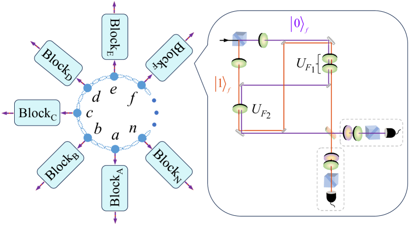
Figure 6: Schematic setup to generate optical entangled state on $N$ separable long-distance qubits.

We also devise an optical scheme for generating entangled states on $N$ separable long-distance photonic qubits, as shown in Fig. 6. A prior $n$-qubit GHZ polarization state $|\Upsilon_{0}\rangle_{ab\ldots n}=\frac{1}{\sqrt{2}}(|H\rangle^{\otimes n}+|V\rangle^{\otimes n})_{ab\ldots n}$ is shared among $N$ parties. Each “Block” transforms the polarization entangled state into the path entangled state $|\Upsilon_{1}\rangle_{ab\ldots n}=\frac{1}{\sqrt{2}}(|0\rangle^{\otimes n}+|1\rangle^{\otimes n})_{ab\ldots n}\otimes|\phi\rangle_{A}\otimes|\phi\rangle_{B}\otimes\ldots\otimes|\phi\rangle_{N}$, where the path DoF acts as control qubit to manipulate the order of the single-qubit gates ($U_{I_{1}}$ and $U_{I_{2}}$) applied on the polarization state $|\phi\rangle_{I}$ ($I=A,B,\dots,N$). Here $|\phi\rangle_{I}=\cos 2\lambda_{i}|H\rangle+\sin 2\lambda_{i}|V\rangle$ denotes a general single-qubit polarization state. Each single-qubit gate $U_{I_{1}}=R_{y}(2\theta)$ can be realized by an HWP rotated at $0^{\circ}$ and an HWP rotated at $\frac{\theta}{2}^{\circ}$, and each single-qubit gate $U_{I_{2}}=X$ can be realized by an HWP rotated at $45^{\circ}$. Finally, the path DoFs of the photons are measured, and the $N$-qubit polarization state can be entangled by selecting the appropriate parameters.

IV Discussion and summary

Our deterministic protocols in principle with unity fidelity and efficiency. However, in actual long-distance photon transmission and manipulation, inevitable experimental errors will be introduced and degrade the efficiency of entanglement preparation. The efficiency of the protocol is mainly affected by the transmission loss and scattering loss of photons in the quantum channel, as well as single photon detection. We assume that the distance between each two parties is $L$. In previous protocols, an $N$-qubit entangled state among distant nodes is generated by using a single photon as a common-data bus to couple with $N$ stationary qubits, resulting in a total optical channel length of $(N-1)L$. Using this approach, the efficiency for generating such an $N$-qubit entangled state is given by Xie et al. (2023); Zhou et al. (2023b); Li et al. (2024)

$$\eta_{N}^{\prime}(L)=\eta_{0}^{N}\eta_{d}\text{exp}[-\alpha(N-1)L].$$ (31)

Here $\eta_{0}=0.96$ is the probability of a photon into the optical channel after scattering in photon-cavity interaction. $\eta_{d}$ is the efficiency of a single-photon detector and $\eta_{d}\geq 0.96$. The exponential term represents photon loss in an optical channel, and $\alpha\simeq\frac{1}{22}$km^-1 is attenuation rate of photon in the optical channel Sangouard et al. (2011).

In contrast, our protocol employs an $N$-photon state that is shared among the $N$ parties. By strategically positioning the shared state at a central location relative to all parties, the total transmission distance of the $N$ photons can be minimized, and the minimum distance is $\frac{N}{2\text{sin}(\frac{\pi}{N})}L$. The scattering loss of a photon in few linear-optics elements in our protocols can be negligible. Therefore, the efficiency of our protocol for generating an $N$-qubit entangled state among $N$ parties is

$$\eta_{N}(L)=\eta_{d}^{N}\text{exp}\bigg{[}-\alpha\frac{N}{2\text{sin}(\frac{\pi}{N})}L\bigg{]}.$$ (32)

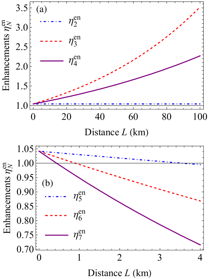
Figure 7: The efficiency enhancements $\eta_{N}^{\text{en}}$ for generating an $N$-qubit long-distance entangled state among $N$ parties. $L$ represents the distance between each pair of parties. (a) The efficiency enhancements for $N=2,3,4$ significantly improve efficiency regardless of the distance $L$. (b) The efficiency enhancements for $N=5,6,7$ improve efficiency when the distance $L$ is small.

We define an efficiency enhancement $\eta_{N}^{\text{en}}(L)=\frac{\eta_{N}(L)}{\eta_{N}^{\prime}(L)}$ to quantify the advantages of our protocols. The enhancement $\eta_{N}^{\text{en}}(L)$ is described by

$$\eta_{N}^{\text{en}}(L)=\eta_{0}^{-N}\eta_{d}^{N-1}\text{exp}\bigg{[}\alpha L\bigg{(}N-1-\frac{N}{2\text{sin}(\frac{\pi}{N})}\bigg{)}\bigg{]}.$$ (33)

The efficiency enhancements as functions of distance $L$ and $N$ are plotted in Fig. 7. As shown in Fig. 7(a), when $N=2,3,4$, all efficiencies are enhanced regardless of the distance $L$. Specially, $\eta_{2}^{\text{en}}(L)=1.042$ for all distances $L$, and $\eta_{2}^{\prime}(11)=53.66\%$ and $\eta_{2}(11)=55.90\%$; $\eta_{2}^{\prime}(66)=4.40\%$ and $\eta_{2}(66)=4.59\%$. When $N=3$ and $N=4$, the efficiencies increase exponentially with the distance $L$ and increases faster for $N=3$. Specially, $\eta_{3}^{\prime}(11)=31.25\%$, $\eta_{3}(11)=37.21\%$, and $\eta_{3}^{\text{en}}(11)=1.191$; $\eta_{3}^{\prime}(66)=0.21\%$, $\eta_{3}(66)=0.49\%$, and $\eta_{3}^{\text{en}}(66)=2.333$; $\eta_{4}^{\prime}(11)=18.19\%$, $\eta_{4}(11)=20.65\%$, and $\eta_{4}^{\text{en}}(11)=1.135$; $\eta_{4}^{\prime}(66)=0.01\%$, $\eta_{4}(66)=0.0175\%$, and $\eta_{4}^{\text{en}}(66)=1.748$. The efficiency enhancements for more qubit entanglement preparation are shown in Fig. 7(b). When $N=5,6,7$, the efficiencies of our protocols can be improved over shorter distances, while the efficiencies will be decreased over longer distances. Specially, when $0<L<3.546$, the efficiency for $N=5$ in our protocol is improved. When $0<L<0.898$, the efficiency for $N=6$ in our protocol is improved. When $0<L<0.435$, the efficiency for $N=7$ in our protocol is improved. Since our protocol involves an $N$-photon state shared among the $N$ parties, it minimizes the total transmission distance of the $N$ photons, resulting in a shorter total distance compared to previous protocols Xie et al. (2023); Zhou et al. (2023b); Li et al. (2024). This reduction in transmission distance leads to lower photon loss, particularly for small $N$, thereby enhancing the overall preparation efficiency.

In summary, we have presented protocols for deterministically generating an $N$-qubit entanglement among $N$ remote parties. A pre-shared maximally entangled state is used to control the orders of single-qubit gates on each target qubit at each party with ICO. Unlike the entanglement swapping technique, our approach avoids multiple pre-shared entanglements and complex entangled state measurements, relying instead on a pre-shared entanglement and simple single-qubit gates, which enhances experimental feasibility and flexibility.

Our protocols can generate long-distance MESs, PESs, and SSs, which depends on the initial state coefficients and angles of single-qubit rotation gates. The entanglement capacity of the output state varies with different parameter choices, and it can be equivalented to different graph or hypergraph states up to local single-qubit unitary transformations Huang et al. (2024). Certain MESs and PESs, corresponding to graph or hypergraph states serve as essential resources for universal measurement-based quantum computation (MBQC) Takeuchi et al. (2019) and distributed quantum computing. They also can simplify the client’s requirement to particularly suit for blind MBQC applications Huang et al. (2024); Zhu and Hayashi (2019).

In addition, we propose compact optical schemes for implementing these protocols by encoding information in the polarization and path DoFs of photons. Unlike previous approaches based on photon-spin interactions Xie et al. (2023); Zhou et al. (2023b); Li et al. (2024), the optical schemes rely on a pre-shared $N$-photon state and the superposition of single-qubit gate operations, offering a fundamentally different approach. This key distinction leads to higher efficiency and simplified state preparation. For example, the efficiencies of our schemes for generating 3-qubit and 4-qubit entanglements are improved exponentially with the distance $L$. For larger numbers of qubits, efficiencies also can be improved over the short distances. This work presents an efficient and practical framework for general entanglement generation among multiple nodes, serving as an essential foundation for the realization of large-scale quantum networks. This advancement paves the way for the development of practical quantum technologies, with potential applications in distributed quantum computing, (blind) MBQC, and long-distance quantum communication.

References

- Horodecki et al. (2009) R. Horodecki, P. Horodecki, M. Horodecki, and K. Horodecki, Quantum entanglement, Rev. Mod. Phys. 81, 865 (2009).
- Jiang et al. (2007) L. Jiang, J. M. Taylor, A. S. Sørensen, and M. D. Lukin, Distributed quantum computation based on small quantum registers, Phys. Rev. A 76, 062323 (2007).
- Oh et al. (2023) E. Oh, X. Lai, J. Wen, and S. Du, Distributed quantum computing with photons and atomic memories, Adv. Quantum Technol. 6, 2300007 (2023).
- Liu et al. (2024a) X. Liu, X.-M. Hu, T.-X. Zhu, C. Zhang, Y.-X. Xiao, J.-L. Miao, Z.-W. Ou, P.-Y. Li, B.-H. Liu, Z.-Q. Zhou, et al., Nonlocal photonic quantum gates over 7.0 km, Nat. Commun. 15, 8529 (2024a).
- Long and Liu (2002) G.-L. Long and X.-S. Liu, Theoretically efficient high-capacity quantum-key-distribution scheme, Phys. Rev. A 65, 032302 (2002).
- Xu et al. (2020) F. Xu, X. Ma, Q. Zhang, H.-K. Lo, and J.-W. Pan, Secure quantum key distribution with realistic devices, Rev. Mod. Phys. 92, 025002 (2020).
- Sheng et al. (2022) Y.-B. Sheng, L. Zhou, and G.-L. Long, One-step quantum secure direct communication, Sci. Bull. 67, 367 (2022).
- Zhou and Sheng (2022) L. Zhou and Y.-B. Sheng, One-step device-independent quantum secure direct communication, Sci. China Phys. Mech. Astron. 65, 250311 (2022).
- Zhou et al. (2023a) L. Zhou, B.-W. Xu, W. Zhong, and Y.-B. Sheng, Device-independent quantum secure direct communication with single-photon sources, Phys. Rev. Appl. 19, 014036 (2023a).
- Zhao et al. (2024) P. Zhao, W. Zhong, M.-M. Du, X.-Y. Li, L. Zhou, and Y.-B. Sheng, Quantum secure direct communication with hybrid entanglement, Front. Phys. 19, 51201 (2024).
- Chaturvedi et al. (2024) A. Chaturvedi, G. Viola, and M. Pawłowski, Extending loophole-free nonlocal correlations to arbitrarily large distances, npj Quantum Inf. 10, 7 (2024).
- Villegas-Aguilar et al. (2024) L. Villegas-Aguilar, E. Polino, F. Ghafari, M. T. Quintino, K. T. Laverick, I. R. Berkman, S. Rogge, L. K. Shalm, N. Tischler, E. G. Cavalcanti, et al., Nonlocality activation in a photonic quantum network, Nat. Commun. 15, 3112 (2024).
- Lobo et al. (2024) E. P. Lobo, J. Pauwels, and S. Pironio, Certifying long-range quantum correlations through routed Bell tests, Quantum 8, 1332 (2024).
- Yin et al. (2020) P. Yin, Y. Takeuchi, W.-H. Zhang, Z.-Q. Yin, Y. Matsuzaki, X.-X. Peng, X.-Y. Xu, J.-S. Xu, J.-S. Tang, Z.-Q. Zhou, et al., Experimental demonstration of secure quantum remote sensing, Phys. Rev. Appl. 14, 014065 (2020).
- Zhao et al. (2021) S.-R. Zhao, Y.-Z. Zhang, W.-Z. Liu, J.-Y. Guan, W. Zhang, C.-L. Li, B. Bai, M.-H. Li, Y. Liu, L. You, et al., Field demonstration of distributed quantum sensing without post-selection, Phys. Rev. X 11, 031009 (2021).
- Malia et al. (2022) B. K. Malia, Y. Wu, J. Martínez-Rincón, and M. A. Kasevich, Distributed quantum sensing with mode-entangled spin-squeezed atomic states, Nature 612, 661 (2022).
- Wang et al. (2018) X.-L. Wang, Y.-H. Luo, H.-L. Huang, M.-C. Chen, Z.-E. Su, C. Liu, C. Chen, W. Li, Y.-Q. Fang, X. Jiang, et al., 18-qubit entanglement with six photons’ three degrees of freedom, Phys. Rev. Lett. 120, 260502 (2018).
- Chen et al. (2024) S. Chen, L.-C. Peng, Y.-P. Guo, X.-M. Gu, X. Ding, R.-Z. Liu, J.-Y. Zhao, X. You, J. Qin, Y.-F. Wang, et al., Heralded three-photon entanglement from a single-photon source on a photonic chip, Phys. Rev. Lett. 132, 130603 (2024).
- Cao et al. (2024) H. Cao, L. M. Hansen, F. Giorgino, L. Carosini, P. Zahálka, F. Zilk, J. C. Loredo, and P. Walther, Photonic source of heralded Greenberger-Horne-Zeilinger states, Phys. Rev. Lett. 132, 130604 (2024).
- Pan et al. (1998) J.-W. Pan, D. Bouwmeester, H. Weinfurter, and A. Zeilinger, Experimental entanglement swapping: entangling photons that never interacted, Phys. Rev. Lett. 80, 3891 (1998).
- de Riedmatten et al. (2005) H. de Riedmatten, I. Marcikic, J. Van Houwelingen, W. Tittel, H. Zbinden, and N. Gisin, Long-distance entanglement swapping with photons from separated sources, Phys. Rev. A 71, 050302 (2005).
- Su et al. (2016) X. Su, C. Tian, X. Deng, Q. Li, C. Xie, and K. Peng, Quantum entanglement swapping between two multipartite entangled states, Phys. Rev. Lett. 117, 240503 (2016).
- Liu et al. (2022) S. Liu, Y. Lou, Y. Chen, and J. Jing, All-optical entanglement swapping, Phys. Rev. Lett. 128, 060503 (2022).
- Chou et al. (2007) C.-W. Chou, J. Laurat, H. Deng, K. S. Choi, H. De Riedmatten, D. Felinto, and H. J. Kimble, Functional quantum nodes for entanglement distribution over scalable quantum networks, Science 316, 1316 (2007).
- Riebe et al. (2008) M. Riebe, T. Monz, K. Kim, A. Villar, P. Schindler, M. Chwalla, M. Hennrich, and R. Blatt, Deterministic entanglement swapping with an ion-trap quantum computer, Nat. Phys. 4, 839 (2008).
- Zopf et al. (2019) M. Zopf, R. Keil, Y. Chen, J. Yang, D. Chen, F. Ding, and O. G. Schmidt, Entanglement swapping with semiconductor-generated photons violates Bell’s inequality, Phys. Rev. Lett. 123, 160502 (2019).
- Ning et al. (2019) W. Ning, X.-J. Huang, P.-R. Han, H. Li, H. Deng, Z.-B. Yang, Z.-R. Zhong, Y. Xia, K. Xu, D. Zheng, et al., Deterministic entanglement swapping in a superconducting circuit, Phys. Rev. Lett. 123, 060502 (2019).
- Couteau (2018) C. Couteau, Spontaneous parametric down-conversion, Contemp. Phys. 59, 291 (2018).
- Lütkenhaus et al. (1999) N. Lütkenhaus, J. Calsamiglia, and K.-A. Suominen, Bell measurements for teleportation, Phys. Rev. A 59, 3295 (1999).
- Calsamiglia and Lütkenhaus (2001) J. Calsamiglia and N. Lütkenhaus, Maximum efficiency of a linear-optical Bell-state analyzer, Appl. Phys. B 72, 67 (2001).
- Bayerbach et al. (2023) M. J. Bayerbach, S. E. D’Aurelio, P. van Loock, and S. Barz, Bell-state measurement exceeding 50% success probability with linear optics, Sci. Adv. 9, eadf4080 (2023).
- Walborn et al. (2003) S. P. Walborn, S. Pádua, and C. H. Monken, Hyperentanglement-assisted Bell-state analysis, Phys. Rev. A 68, 042313 (2003).
- Barbieri et al. (2007) M. Barbieri, G. Vallone, P. Mataloni, and F. De Martini, Complete and deterministic discrimination of polarization Bell states assisted by momentum entanglement, Phys. Rev. A 75, 042317 (2007).
- Williams et al. (2017) B. P. Williams, R. J. Sadlier, and T. S. Humble, Superdense coding over optical fiber links with complete Bell-state measurements, Phys. Rev. Lett. 118, 050501 (2017).
- Zhou et al. (2022) X.-J. Zhou, W.-Q. Liu, H.-R. Wei, Y.-B. Zheng, and F.-F. Du, Deterministic and complete hyperentangled Bell states analysis assisted by frequency and time interval degrees of freedom, Front. Phys. 17, 41502 (2022).
- Sheng et al. (2010) Y.-B. Sheng, F.-G. Deng, and G. L. Long, Complete hyperentangled-Bell-state analysis for quantum communication, Phys. Rev. A 82, 032318 (2010).
- Li and Ghose (2016) X.-H. Li and S. Ghose, Complete hyperentangled Bell state analysis for polarization and time-bin hyperentanglement, Opt. Express 24, 18388 (2016).
- Li et al. (2019) T. Li, A. Miranowicz, K. Xia, and F. Nori, Resource-efficient analyzer of Bell and Greenberger-Horne-Zeilinger states of multiphoton systems, Phys. Rev. A 100, 052302 (2019).
- Callus and Kok (2021) E. Callus and P. Kok, Cumulative generation of maximal entanglement between spectrally distinct qubits using squeezed light, Phys. Rev. A 104, 052407 (2021).
- Li et al. (2018) T. Li, A. Miranowicz, X. Hu, K. Xia, and F. Nori, Quantum memory and gates using a -type quantum emitter coupled to a chiral waveguide, Phys. Rev. A 97, 062318 (2018).
- Li et al. (2016) T. Li, G.-J. Yang, and F.-G. Deng, Heralded quantum repeater for a quantum communication network based on quantum dots embedded in optical microcavities, Phys. Rev. A 93, 012302 (2016).
- Sangouard et al. (2011) N. Sangouard, C. Simon, H. De Riedmatten, and N. Gisin, Quantum repeaters based on atomic ensembles and linear optics, Rev. Mod. Phys. 83, 33 (2011).
- Munro et al. (2012) W. J. Munro, A. M. Stephens, S. J. Devitt, K. A. Harrison, and K. Nemoto, Quantum communication without the necessity of quantum memories, Nat. Photon. 6, 777 (2012).
- Wu et al. (2022) J. Wu, G.-L. Long, and M. Hayashi, Quantum secure direct communication with private dense coding using a general preshared quantum state, Phys. Rev. Appl. 17, 064011 (2022).
- Xie et al. (2023) Z. Xie, G. Wang, Z. Guo, Z. Li, and T. Li, Heralded quantum multiplexing entanglement between stationary qubits via distribution of high-dimensional optical entanglement, Opt. Express 31, 37802 (2023).
- Zhou et al. (2023b) H. Zhou, T. Li, and K. Xia, Parallel and heralded multiqubit entanglement generation for quantum networks, Phys. Rev. A 107, 022428 (2023b).
- Li et al. (2024) J. Li, Z. Xie, Y. Li, Y. Liang, Z. Li, and T. Li, Heralded entanglement between error-protected logical qubits for fault-tolerant distributed quantum computing, Sci. China-Phys. Mech. Astron. 67, 220311 (2024).
- Lo Piparo et al. (2019) N. Lo Piparo, W. J. Munro, and K. Nemoto, Quantum multiplexing, Phys. Rev. A 99, 022337 (2019).
- Bernien et al. (2013) H. Bernien, B. Hensen, W. Pfaff, G. Koolstra, M. S. Blok, L. Robledo, T. H. Taminiau, M. Markham, D. J. Twitchen, L. Childress, et al., Heralded entanglement between solid-state qubits separated by three metres, Nature 497, 86 (2013).
- van Leent et al. (2022) T. van Leent, M. Bock, F. Fertig, R. Garthoff, S. Eppelt, Y. Zhou, P. Malik, M. Seubert, T. Bauer, W. Rosenfeld, et al., Entangling single atoms over 33 km telecom fibre, Nature 607, 69 (2022).
- Krutyanskiy et al. (2023) V. Krutyanskiy, M. Galli, V. Krcmarsky, S. Baier, D. Fioretto, Y. Pu, A. Mazloom, P. Sekatski, M. Canteri, M. Teller, et al., Entanglement of trapped-ion qubits separated by 230 meters, Phys. Rev. Lett. 130, 050803 (2023).
- Wei et al. (2019) K. Wei, N. Tischler, S.-R. Zhao, Y.-H. Li, J. M. Arrazola, Y. Liu, W. Zhang, H. Li, L. You, Z. Wang, et al., Experimental quantum switching for exponentially superior quantum communication complexity, Phys. Rev. Lett. 122, 120504 (2019).
- Nie et al. (2022) X. Nie, X. Zhu, K. Huang, K. Tang, X. Long, Z. Lin, Y. Tian, C. Qiu, C. Xi, X. Yang, et al., Experimental realization of a quantum refrigerator driven by indefinite causal orders, Phys. Rev. Lett. 129, 100603 (2022).
- Yin et al. (2023) P. Yin, X. Zhao, Y. Yang, Y. Guo, W.-H. Zhang, G.-C. Li, Y.-J. Han, B.-H. Liu, J.-S. Xu, G. Chiribella, et al., Experimental super-Heisenberg quantum metrology with indefinite gate order, Nat. Phys. 19, 1122 (2023).
- Liu et al. (2024b) W. Q. Liu, Z. Meng, B. W. Song, J. Li, Q. Y. Wu, X. X. Chen, J. Y. Hong, A. N. Zhang, and Z. Q. Yin, Experimentally demonstrating indefinite causal order algorithms to solve the generalized Deutsch’s problem, Adv. Quantum Technol. 7, 2400181 (2024b).
- Liu and Wei (2025) W.-Q. Liu and H.-R. Wei, Quantum gate teleportation with the superposition of causal order, Phys. Rev. Appl. 23, 014064 (2025).
- Chiribella et al. (2013) G. Chiribella, G. M. D’Ariano, P. Perinotti, and B. Valiron, Quantum computations without definite causal structure, Phys. Rev. A 88, 022318 (2013).
- Chiribella et al. (2021) G. Chiribella, M. Banik, S. S. Bhattacharya, T. Guha, M. Alimuddin, A. Roy, S. Saha, S. Agrawal, and G. Kar, Indefinite causal order enables perfect quantum communication with zero capacity channels, New J. Phys. 23, 033039 (2021).
- Kechrimparis et al. (2024) S. Kechrimparis, J. Moran, A. Karsa, C. Lee, and H. Kwon, Enhancing quantum state discrimination with indefinite causal order, New J. Phys. 26, 123030 (2024).
- Procopio et al. (2015) L. M. Procopio, A. Moqanaki, M. Araújo, F. Costa, I. Alonso Calafell, E. G. Dowd, D. R. Hamel, L. A. Rozema, Č. Brukner, and P. Walther, Experimental superposition of orders of quantum gates, Nat. Commun. 6, 7913 (2015).
- Goswami et al. (2018) K. Goswami, C. Giarmatzi, M. Kewming, F. Costa, C. Branciard, J. Romero, and A. G. White, Indefinite causal order in a quantum switch, Phys. Rev. Lett. 121, 090503 (2018).
- Guo et al. (2020) Y. Guo, X.-M. Hu, Z.-B. Hou, H. Cao, J.-M. Cui, B.-H. Liu, Y.-F. Huang, C.-F. Li, G.-C. Guo, and G. Chiribella, Experimental transmission of quantum information using a superposition of causal orders, Phys. Rev. Lett. 124, 030502 (2020).
- Strömberg et al. (2023) T. Strömberg, P. Schiansky, R. W. Peterson, M. T. Quintino, and P. Walther, Demonstration of a quantum switch in a Sagnac configuration, Phys. Rev. Lett. 131, 060803 (2023).
- Rozema et al. (2024) L. A. Rozema, T. Strömberg, H. Cao, Y. Guo, B.-H. Liu, and P. Walther, Experimental aspects of indefinite causal order in quantum mechanics, Nat. Rev. Phys. 6, 483 (2024).
- Kwiat et al. (1999) P. G. Kwiat, E. Waks, A. G. White, I. Appelbaum, and P. H. Eberhard, Ultrabright source of polarization-entangled photons, Phys. Rev. A 60, R773 (1999).
- Zhang et al. (2021) C. Zhang, Y.-F. Huang, B.-H. Liu, C.-F. Li, and G.-C. Guo, Spontaneous parametric down-conversion sources for multiphoton experiments, Adv. Quantum Technol. 4, 2000132 (2021).
- Jin et al. (2014) R.-B. Jin, R. Shimizu, K. Wakui, M. Fujiwara, T. Yamashita, S. Miki, H. Terai, Z. Wang, and M. Sasaki, Pulsed Sagnac polarization-entangled photon source with a PPKTP crystal at telecom wavelength, Optics Express 22, 11498 (2014).
- Lee et al. (2016) S. M. Lee, H. Kim, M. Cha, and H. S. Moon, Polarization-entangled photon-pair source obtained via type-II non-collinear SPDC process with PPKTP crystal, Opt. Express 24, 2941 (2016).
- Chen et al. (2020) Y. Chen, S. Ecker, J. Bavaresco, T. Scheidl, L. Chen, F. Steinlechner, M. Huber, and R. Ursin, Verification of high-dimensional entanglement generated in quantum interference, Phys. Rev. A 101, 032302 (2020).
- Huang et al. (2024) J. Huang, X. Li, X. Chen, C. Zhai, Y. Zheng, Y. Chi, Y. Li, Q. He, Q. Gong, and J. Wang, Demonstration of hypergraph-state quantum information processing, Nat. Commun. 15, 2601 (2024).
- Takeuchi et al. (2019) Y. Takeuchi, T. Morimae, and M. Hayashi, Quantum computational universality of hypergraph states with Pauli-X and Z basis measurements, Sci. Rep. 9, 13585 (2019).
- Zhu and Hayashi (2019) H. Zhu and M. Hayashi, Efficient verification of hypergraph states, Phys. Rev. Appl. 12, 054047 (2019).