Dynamics in Hamiltonian Lattice Gauge Theory: Approaching the Continuum Limit with Partitionings of SU$(2)$

Abstract

In this paper, we investigate a digitised SU$(2)$ lattice gauge theory in the Hamiltonian formalism. We use partitionings to digitise the gauge degrees of freedom and show how to define a penalty term based on finite element methods to project onto physical states of the system. Moreover, we show for a single plaquette system that in this framework the limit $g\to 0$ can be approached at constant cost.

I Introduction

The implementation of SU$(N)$ lattice gauge theories in the original formulation by Kogut and Susskind Kogut and Susskind (1975) is notoriously difficult on both classical and quantum computers, at least if one is interested in the limit of gauge coupling $g\to 0$, corresponding to the continuum limit of the lattice theory. In combination with local gauge invariance, the non-Abelian structure of such theories and the practical requirement for digitization and truncation lead to non-localities in formulations suitable for this limit, or severe increase in resource requirements.

While the widely used Clebsch-Gordan expansion Zohar and Burrello (2015) is working well at large $g$, it is not well suited for the limit of $g\to 0$: the number of terms required in the expansion grows quickly with decreasing values of $g$. The reason for this behaviour is likely the fact that the electric part of the Hamiltonian is diagonal in this formulation, which becomes less and less dominant in the foreseen limit.

Therefore, there is a significant effort to construct a basis in which the magnetic part of the Hamiltonian is diagonal, which in general involves some kind of gauge fixing and a suitable basis choice for the gauge field degrees of freedom. Recently, in Ref. Grabowska et al. (2024) a fully gauge fixed SU$(2)$ Hamiltonian has been developed, based on ideas worked out in Ref. D’Andrea et al. (2024). While the latter approach involves a functional basis, the works in Refs. Gustafson et al. (2022, 2024) are based on discrete tetrahedral and octahedral sub-groups of SU$(2)$. Also, in Ref. Burbano and Bauer (2024) a Gauge Loop-String-Hadron formulation is developed on general graphs. For earlier work see for instance Refs. Ji et al. (2020); Alexandru et al. (2019, 2022); Ji et al. (2023). Of course, one can also try to find alternative Hamiltonians to the one derived by Kogut and Susskind. Examples are quantum link models Chandrasekharan and Wiese (1997); Brower et al. (1999); Wiese (2021), a Hamiltonian based on a Heisenberg-Comb Bhattacharya et al. (2021) or the orbifold approach presented in Bergner et al. (2024).

In Ref. Jakobs et al. (2023a) we have presented a formulation using partitionings of SU$(2)$ based on Ref. Hartung et al. (2022) (see also Refs. Jakobs et al. (2023b); Garofalo et al. (2024)), which has the advantage that the number of elements can be chosen freely while working in the magnetic basis. In these references we have shown how the canonical momenta and in particular their square can be constructed based on finite element methods. We have tested this approach in the free theory and found that the continuum energy levels and eigenstates are recovered in the limit of continuous gauge symmetry. The disadvantage of this approach is that gauge invariance is realised only approximatively. For ways to mitigate this see Ref. Romiti and Urbach (2024).

In this paper we will use the same formalism and investigate its behaviour in the interacting theory: for this, we show how to construct the Gauss operator again based on finite element methods. This Gauss operator can then be used to construct a penalty term, which lets one single out the physically relevant states. We also introduce a truncation which makes it possible to take the limit of gauge coupling $g^{2}\to 0$ (continuum limit) at constant cost and constant error stemming from the group discretisation. This is exemplified for a single plaquette system in the maximal tree gauge.

II Theory

The Kogut and Susskind Hamiltonian Kogut and Susskind (1975) of lattice gauge theory we alluded to in the previous section is defined on a cubical lattice, discretising the spatial dimensions only. Similarly to Wilson’s famous Lagrangian formulation of lattice gauge theories Wilson (1974), the gauge degrees of freedom take the form of links connecting the spatial lattice sites. Each link is classically described by a colour matrix $U$ in the fundamental representation of the gauge group $G$.

Quantum states of the system are described by a wave function

$$\psi\left(\left\{U_{\mathbf{x},k}\right\}\right):G^{N_{\textrm{links}}}\,\,\rightarrow\,\,\mathbb{C}\,,$$ (1)

assigning a complex probability amplitude to every classical configuration $\left\{U_{\mathbf{x},k}\right\}$ of the gauge links. The indices $\mathbf{x}$ and $k$ here label the location and direction of each link.

II.1 Operators

Figure 1: Sketch of the plaquette operator $\hat{P}_{\mathbf{x},ij}$.

To define the Kogut-Susskind Hamiltonian operators $\hat{U}_{\mathbf{x},k}$ are introduced, defined by the action

$$\hat{U}_{\mathbf{x},k}\,\psi=U_{\mathbf{x},k}\ \psi\left(\dots,{U_{\mathbf{x},k}},\dots\right)$$ (2)

on wave functions $\psi$, with $\hat{U}^{\dagger}\hat{U}^{~}=1$ and $\mathrm{det}\hat{U}=1$. Like the position operator in quantum mechanics the link operator modifies the wave function by multiplying with the gauge link degree of freedom labelled by $\mathbf{x}$ and $k$. $\hat{U}$ and $\hat{U}^{\dagger}$ can then be combined to define the plaquette operator $\hat{P}$. As depicted in fig. 1 it connects four gauge links to an oriented loop:

$$\hat{P}_{\mathbf{x},ij}=\ \hat{U}_{\mathbf{x},i}\,\hat{U}_{\mathbf{x}+a\hat{\mathbf{i}},j}\,\hat{U}^{\dagger}_{\mathbf{x}+a\hat{\mathbf{j}},i}\,\hat{U}^{\dagger}_{\mathbf{x},j}\,.$$ (3)

Furthermore, we define the left and right momentum operators $\hat{L}^{c}_{\mathbf{x},k}$ and $\hat{R}^{c}_{\mathbf{x},k}$. They take the shape of Lie derivatives and are defined as

$$\hat{L}^{c}_{\mathbf{x},k}\,\psi\ =-\operatorname{i}\frac{\mathrm{d}}{\mathrm{d}\beta}\,\psi\left(\dots,e^{-\operatorname{i}\beta t_{c}}\,U_{\mathbf{x},k},\dots\right)|_{\beta=0}\,$$ (4)

and

$$\hat{R}^{c}_{\mathbf{x},k}\,\psi\ =-\operatorname{i}\frac{\mathrm{d}}{\mathrm{d}\beta}\,\psi\left(\dots,U_{\mathbf{x},k}\,e^{\operatorname{i}\beta t_{c}},\dots\right)|_{\beta=0}\,,$$ (5)

where the $t_{c}$ denote the generators of the gauge group. The momentum operators obey the following canonical commutation relations

$$[\hat{L}^{c}_{\mathbf{x},i},\hat{U}_{\mathbf{y},j}]\ =\ -\delta_{\mathbf{x}\mathbf{y}}\,\delta_{ij}\,t_{c}\,\hat{U}_{\mathbf{x},i}\,,$$ (6)

$$[\hat{R}^{c}_{\mathbf{x},i},\hat{U}_{\mathbf{y},j}]\ =\ \delta_{\mathbf{x}\mathbf{y}}\,\delta_{ij}\,\hat{U}_{\mathbf{x},i}\,t_{c}\,,$$ (7)

and

$$[\hat{L}^{a}_{\mathbf{x},i},\hat{L}^{b}_{\mathbf{y},j}] =\operatorname{i}f_{abc}\,\delta_{\mathbf{x}\mathbf{y}}\,\delta_{ij}\,\hat{L}^{c}\,$$ (8)

$$[\hat{R}^{a}_{\mathbf{x},i},\hat{R}^{b}_{\mathbf{y},j}] =\operatorname{i}f_{abc}\,\delta_{\mathbf{x}\mathbf{y}}\,\delta_{ij}\,\hat{R}^{c}\,.$$ (9)

Here $f_{abc}$ are the structure constants of the gauge group.

II.2 The Hamiltonian

With these ingredients the Kogut-Susskind Hamiltonian for a pure lattice gauge theory reads

$$\begin{split}\hat{H}&=\ \frac{g^{2}}{2}\sum_{\mathbf{x},c,k}\left(\hat{L}_{\mathbf{x},k}^{c}\right)^{2}+\frac{2}{g^{2}}\sum_{\mathbf{x},j<i}\mathrm{Tr}\left[\,\mathbb{1}-\mathrm{Re}\,\hat{P}_{\mathbf{x},ij}\right]\,.\end{split}$$ (10)

The first term encodes the local kinetic energy and is typically referred to as the electric term. Its ground state is

$$\psi_{0}^{\textrm{el.}}\left(\left\{U_{\mathbf{x},k}\right\}\right)=\mathrm{const}\,.$$ (11)

The second term implements an interaction between the four links of each plaquette and is typically referred to as the magnetic term. Its ground state reads

$$\psi_{0}^{\textrm{mag.}}\left(\left\{U_{\mathbf{x},k}\right\}\right)=\prod_{\mathbf{x},i<j}\delta(\mathbb{1}-P_{\mathbf{x},ij})\,.$$ (12)

The physical Hilbert space of the theory is further restricted by a constraint referred to as Gauss law. It states that any physical state $\ket{\psi}$ needs to satisfy

$$\hat{G}^{c}_{\mathbf{x}}\ket{\psi}=\sum_{k}\left(\hat{L}^{c}_{\mathbf{x},k}+\hat{R}^{c}_{\mathbf{x}-a\hat{\mathbf{k}},k}\right)\ket{\psi}=0\,.$$ (13)

This can be understood as demanding colour charge conservation at each vertex in the lattice. It significantly reduces the dimensionality of the Hilbert space of the theory.

II.3 Dual Formulation

By considering the ground states of the electric and magnetic parts of the Hamiltonian alone, respectively, we can make some educated guesses about the ground state of the full Hamiltonian. For large $g^{2}$ we expect it to be quite uniform with little entanglement between the links. This is because here we mostly have a free theory, perturbed by a weak potential implemented by the magnetic term.

When decreasing $g^{2}$ the entanglement between links increases with the wave function only being non-vanishing for configurations where all the $P_{\mathbf{x},ij}\approx\mathbb{1}$. All other configurations will be suppressed due to the then large $1/g^{2}$. Thus, it would be highly beneficial to rewrite the Hamiltonian in terms of plaquette degrees of freedom instead of the original gauge links

$$\psi\left(\left\{U_{\mathbf{x},i}\right\}\right)\rightarrow\psi\left(\left\{P_{\mathbf{x},ij}\right\}\right)\,,$$ (14)

which would lead to a magnetic term, consisting of a sum of single site operators and nearest neighbour interactions in the electric term. As a result, the entanglement between the individual degrees of freedom would no longer increase for $g^{2}\rightarrow 0$. Furthermore, one could now make use of the fact that the wave function of the system only is non-vanishing for $P_{\mathbf{x},ij}$ close to the identity. This could be exploited by choosing a basis for the wavefunctions that is suitable for approximating wavefunctions distributed around $P_{\mathbf{x},ij}=\mathbb{1}$ well.

While this idea can be implemented in an Abelian U$(1)$ theory, it is obfuscated in non-Abelian theories by their non-commutative nature, which makes it necessary to add additional terms to the Hamiltonian, which introduce non-localities. For SU$(N)$ multiple dual Hamiltonians are under consideration D’Andrea et al. (2024); Ligterink et al. (2000a); Mathur and Rathor (2023).

Since this is not the focus of this paper, we avoid this complication by studying a single plaquette lattice only. By squaring Gauss’ law it is easy to show that

$$\sum_{c}(\hat{L}_{1}^{c})^{2}=\sum_{c}(\hat{L}_{2}^{c})^{2}=\sum_{c}(\hat{L}_{3}^{c})^{2}=\sum_{c}(\hat{L}_{4}^{c})^{2}\,,$$ (15)

where the indices 1,2,3 and 4 label the four links in the plaquette. Thus, one can express the Hamiltonian in terms of a single gauge degree of freedom (equivalent to the single plaquette operator)

$$\hat{H}=2g^{2}\sum_{c}(\hat{L}^{c})^{2}+\frac{2}{g^{2}}\mathrm{Tr}\left[\mathbb{1}-\hat{U}\right]\,.$$ (16)

The remaining Gauss law constraint at the origin then takes the shape of

$$\hat{Q}^{c}\ket{\psi}=(\hat{L}^{c}+\hat{R}^{c})\ket{\psi}=0\,.$$ (17)

In the following we will enforce Gauss’ law by adding a penalty term

$$\hat{H}_{\textrm{penalty}}\ =\ \kappa\sum_{c}\left(\hat{Q}^{c}\right)^{2}$$ (18)

to the Hamiltonian of the theory. Here, $\kappa$ is a large positive constant. Such a penalty term will shift unphysical states to higher energiesHalimeh and Hauke (2020), allowing for simulations of the low-lying physical spectrum of the theory.

Furthermore, it is analytically known D’Andrea et al. (2024) that the physical states are the ground state and the fourth excited state of the unconstrained Hamiltonian. Therefore, this system also allows us to study the practicability of using a penalty term.

The gauge group of interest in the following is SU$(2)$. Thus, the generators are given by $t_{c}=\frac{1}{2}\sigma_{c}$, where $\sigma_{c}$ are the Pauli matrices. The structure constants $f_{abc}$ are the components of the Levi-Civita tensor. SU$(2)$ serves as a useful toy model to explore the challenges surrounding Hamiltonian simulations with non-abelian gauge groups. The lessons learned here should hopefully lead the way to Hamiltonian simulations of quantum chromodynamics.

III Discretising the Operators

As the Hilbert space of wave functions is in principle infinite-dimensional, in general a discretisation and possibly a truncation is needed for a practical numerical simulation. The full Hilbert space of the theory can be decomposed into products of wave functions on single gauge links

$$\ket{\{f_{\mathbf{x},k}\}}=\bigotimes_{\mathbf{x},k}\ket{f_{\mathbf{x},k}}\,.$$ (19)

Thus, it is sufficient to find discretisation schemes for the single link wave functions

$$f_{\mathbf{x},k}(U):G\rightarrow\mathbb{C}\,.$$ (20)

More specifically, we will use the finite element canonical momenta we presented in Ref. Jakobs et al. (2023a). The idea here is to approximate each link wave function at a finite set of gauge group elements

$$\left\{D_{i}\right\}\subset\mathrm{SU}(2)\,.$$ (21)

In the following we will refer to such a subset as a partitioning of SU$(2)$. Any such partitioning can be connected to a simplical mesh $\{(i_{0},i_{1},i_{2},i_{3})\}$ via a Delaunay triangulation Delaunay (1934). Here, the integers $i_{j}$ label the four group elements spanning each simplex in the mesh.

Next one can introduce the basis functions $\hat{\phi}_{i}$ with the property

$$\hat{\phi}_{i}(D_{j})=\delta_{ij}\,,$$ (22)

and interpolate linearly inside each simplex of the mesh. Within each simplex we introduce local coordinates $\vec{\alpha}_{L/R}$ defined by

$$U=\exp\left(-\operatorname{i}\vec{\alpha}_{L}\cdot\vec{t}\,\right)D_{i_{0}}$$ (23)

and

$$U=D_{i_{0}}\exp\left(\operatorname{i}\vec{\alpha}_{R}\cdot\vec{t}\,\right)\,,$$ (24)

respectively. The local coordinates are chosen such that the left and right canonical momentum operators take the shape of the components of Lie derivatives on $S_{3}$. By Taylor expanding the function around the value at each vertex, one can calculate the Lie derivatives within each cell to be defined by

$$\begin{pmatrix}\vec{\alpha}_{1,L/R}^{T}\\ \vec{\alpha}_{2,L/R}^{T}\\ \vec{\alpha}_{3,L/R}^{T}\end{pmatrix}\vec{\nabla}_{C,L/R}\,f=\begin{pmatrix}f(D_{i_{1}})-f(D_{i_{0}})\\ f(D_{i_{2}})-f(D_{i_{0}})\\ f(D_{i_{3}})-f(D_{i_{0}})\end{pmatrix}\,,$$ (25)

where $\vec{\alpha}^{T}_{j}$ denotes the coordinates of the vertices $D_{i_{j}}$ found in the simplex $C$. To then further improve the estimate of the momentum operators at a given vertex, one can average the Lie derivative over the simplices surrounding a given vertex. In our implementation this average is weighted by each cell’s volume. The operator matrices are thus calculated as

$$\begin{pmatrix}\hat{L}^{1}_{ij}\\ \hat{L}^{2}_{ij}\\ \hat{L}^{3}_{ij}\end{pmatrix}=\frac{-\operatorname{i}}{\sum_{\{C|i\in C\}}\mathrm{Vol(C)}}\sum_{\{C|i\in C\}}\mathrm{Vol(C)}\,\,\vec{\nabla}_{C,L}\hat{\phi}_{j}\,.$$ (26)

Using the $L^{a}$ operators obtained above to construct the Laplacian operator $\sum_{c}(\hat{L}^{c})^{2}$ will result in a poor approximation because the $L^{a}$ construction relies on a linear approximation. A direct construction of the Laplacian operator $\sum_{c}(\hat{L}^{c})^{2}$ can be obtained as in Jakobs et al. (2023a)

$$\sum_{c}\left(\hat{L}^{c}\right)^{2}=\frac{1}{v(i)}\sum_{\{C\in\mathcal{C}|i,j\in C\}}(\vec{\nabla}_{C}\hat{\phi}_{i})\cdot(\vec{\nabla}_{C}\hat{\phi}_{j})\,\mathrm{Vol}(C)\,.$$ (27)

where $v(i)$ here denotes the barycentric weight at vertex $i$. They are obtained by equally distributing the volume of each simplex onto its vertices

$$v(i)=\frac{1}{4}\sum_{\{C|i\in C\}}\mathrm{Vol}(C)\,.$$ (28)

Again, using the $\hat{L}$ and $\hat{R}$ operators naïvely to construct the squared Gauss operator needed for the penalty term leads to a large artefacts. However, similarly to the Laplacian, also the squared Gauss operator

$$\sum_{c}\hat{Q}_{c}^{2}=\sum_{c}\left(\hat{L}_{c}+\hat{R}_{c}\right)^{2}\,.$$ (29)

can be constructed directly. One obtains

$$\begin{split}\sum_{c}\left(\hat{Q}^{c}\right)^{2}&=\frac{1}{v(i)}\sum_{\{C\in\mathcal{C}|i,j\in C\}}\,\mathrm{Vol}(C)\\ &((\vec{\nabla}_{C,L}+\vec{\nabla}_{C,R})\hat{\phi}_{i})\cdot((\vec{\nabla}_{C,L}+\vec{\nabla}_{C,R})\hat{\phi}_{j})\,.\end{split}$$ (30)

Here $\vec{\nabla}_{C,L}$($\vec{\nabla}_{C,R}$) denote the cell gradient taken in the left (right) local coordinates.

All these momentum operators are local in the sense that a given vertex is only ever mapped to vertices it shares a simplex with. Furthermore, the gauge link operator $\hat{U}$ is diagonal in this basis. However, for these operators the canonical commutation relations and the low-lying spectrum are only exactly recovered in the limit of infinitely fine meshes. For a finite set of gauge group elements the canonical commutation relation are only approximatively fulfilled.

III.1 SU$(2)$ Partitioning

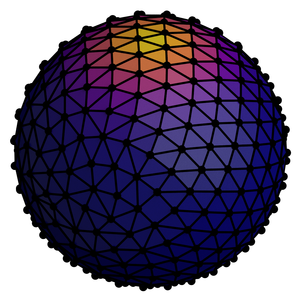
$\rightarrow$

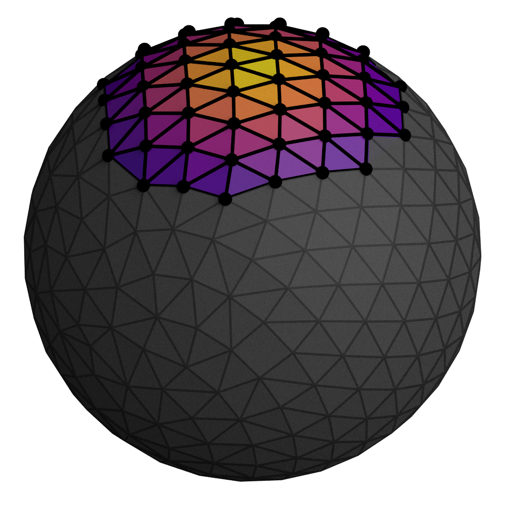
Figure 2: Sketch of the truncation procedure used in the dual Hamiltonian: On the left sphere we show the expected shape of the plaquette wave function towards weaker coupling. Warmer colours symbolise bigger probability amplitudes in the wavefunction. By using partitionings fulfilling eq. 36, we effectively restrict our simulations to a cone surrounding the north-pole of the sphere. This is shown on the right. Note that SU(2) is isomorphic to the 3-sphere embedded in four dimensions, i.e. the pictures shown here should be understood as a lower dimensional sketch of the procedure.

In the following we will use the rotated simple cubic (RSC) partitionings. These are obtained by constructing a simple cubical lattice in the unit cube:

$$\Lambda_{n}^{\textrm{SC}}=\left\{\vec{x}\in[0,1)^{3}\,\middle|\,\vec{x}=d_{\textrm{SC}}(n)\,\textrm{R}\,\vec{m}+\vec{a}\,,\vec{m}\in\mathbb{Z}^{3}\right\}\,.$$ (31)

Here $n$ denotes the target number of points in the lattice. $d_{\textrm{SC}}(n)$ is the distance between neighbouring points given by

$$d_{\textrm{SC}}(n)=n^{-1/3}\,.$$ (32)

The rotation matrix R is needed to ensure that the planes of the lattice are not aligned with the faces of the unit cube. In our implementation successive rotations of $\pi/8$ around $\hat{e}_{1}$,$\hat{e}_{2}$ and $\hat{e}_{3}$ seem to work well. The vector $\vec{a}$ is tuned such that the number of points actually in the cube equals the target $n$.

This lattice is then mapped SU(2) via the volume preserving map:

$$\begin{split}\rho(x_{1})&=\Phi_{1}(x_{1})\,,\\ \theta(x_{2})&=\cos^{-1}\left(1-2\,x_{2}\right)\\ \text{and}\qquad\phi(x_{3})&=2\pi x_{3}\,.\end{split}$$ (33)

Here the function $\Phi_{1}(\rho)$ is defined via its inverse

$$\Phi_{1}^{-1}(\rho)=\frac{1}{\pi}\left(\rho-\frac{1}{2}\sin(2\rho)\right)\,.$$ (34)

The angles $(\rho,\theta,\phi)$ parametrise an SU(2) elements by

$$U(\rho,\theta,\phi)=\cos\rho\mathbb{1}+\operatorname{i}\sin\rho\,\vec{e}_{\rho}(\theta,\phi)\cdot\vec{\sigma}\,,$$ (35)

where $\vec{e}_{\rho}(\theta,\phi)=(\sin\theta\cos\phi,\sin\theta\sin\phi,\cos\theta)$ is a point on $S_{2}$. For more details we refer to Jakobs et al. (2023a); Hartung et al. (2022).

Moreover, as depicted in fig. 2, we expect the plaquette wave function of low-lying states at weak couplings to vanish for points far away from $\mathbb{1}$. For this purpose we implement a truncation by modifying the volume preserving map such that

$$\mathrm{Tr}\left[D_{i}\right]\geq 2\cos\left(\pi\varepsilon_{\mathrm{Tr}}\right)\,.$$ (36)

Here the parameter $\varepsilon_{\mathrm{Tr}}\in(0,1]$ controls how much of the gauge group is approximated by the partitioning around the identity. $\varepsilon_{\mathrm{Tr}}=1$ gives points covering the entire group, while $\varepsilon_{\mathrm{Tr}}=0$ only allows for $D_{i}=\mathbb{1}$.

In the following we will denote different partitionings as RSC${}_{N}^{\varepsilon_{\mathrm{Tr}}}$ describing a set of $N$ points found within the hypersphere cap defined by eq. 36.

c

IV Numerical Results

To study the performance of the proposed discretisation scheme, the ground state and first excited state for the single plaquette system are determined via exact diagonalisation. Gauss’ law will be enforced either by manual selection of the correct states or by the penalty term eq. 18.

As observables, we will consider the ground state energy $E_{0}$, the mass gap $M$ defined as

$$M=E_{1}-E_{0}$$ (37)

and the ground state plaquette expectation value

$$\langle P\rangle\ =\ \frac{1}{2\,N_{\textrm{Plaq}}}\,\sum_{\mathbf{x},i<j}\mathrm{Tr}\left[\bra{\psi_{0}}\hat{P}_{\mathbf{x},ij}\ket{\psi_{0}}\right]\,.$$ (38)

Our numerical results can be compared to the analytic solution derived in Ref. Ligterink et al. (2000b). There the energy levels are calculated to be

$$E_{n}=\frac{4}{g^{2}}+\frac{g^{2}}{8}\left(b_{2n}\left(-16/g^{4}\right)-4\right)\,.$$ (39)

Here $b_{n}$ denotes the Mathieu characteristic numbers. Note that some of the prefactors differ from the cited source due to a difference in convention used for the Hamiltonian. The theoretical prediction of the plaquette expectation value is obtained by numerically integrating the eigenfunctions also given in Ref. Ligterink et al. (2000b).

IV.1 Tuning the Penalty Term

For simulations with a penalty term eq. 18, a value for the parameter $\kappa$ needs to be chosen. For formulations with only approximative gauge invariance, this can be delicate. Since $\hat{Q}^{c}$ only approximates the exact Gauss operator, $\hat{Q}^{c}|\psi\rangle$ can be non-zero even for a physical wave function $|\psi\rangle$. While this is expected to be a small effect in $\hat{Q}^{c}|\psi\rangle$, large values of $\kappa$ can inflate it. Thus, $\kappa$ should not be chosen much larger than needed to move unphysical states beyond the energies of interest. Otherwise, the ground state of the total system will simply be the one with the most favourable discretisation error.

Furthermore, much better matching with the analytic predictions can be achieved, when correcting for energy contributions by the penalty term. This is done by simply subtracting the expectation value of the penalty term from the eigenvalues obtained from the solver:

$$E_{i}=\lambda_{i}-\langle H_{\textrm{penalty}}\rangle\,.$$ (40)

One way to test whether $\kappa$ is sufficiently large is to study the expectation value of $\hat{H}_{\textrm{penalty}}$. This shows a sharp drop, once the unphysical states are projected out.

IV.2 Overview

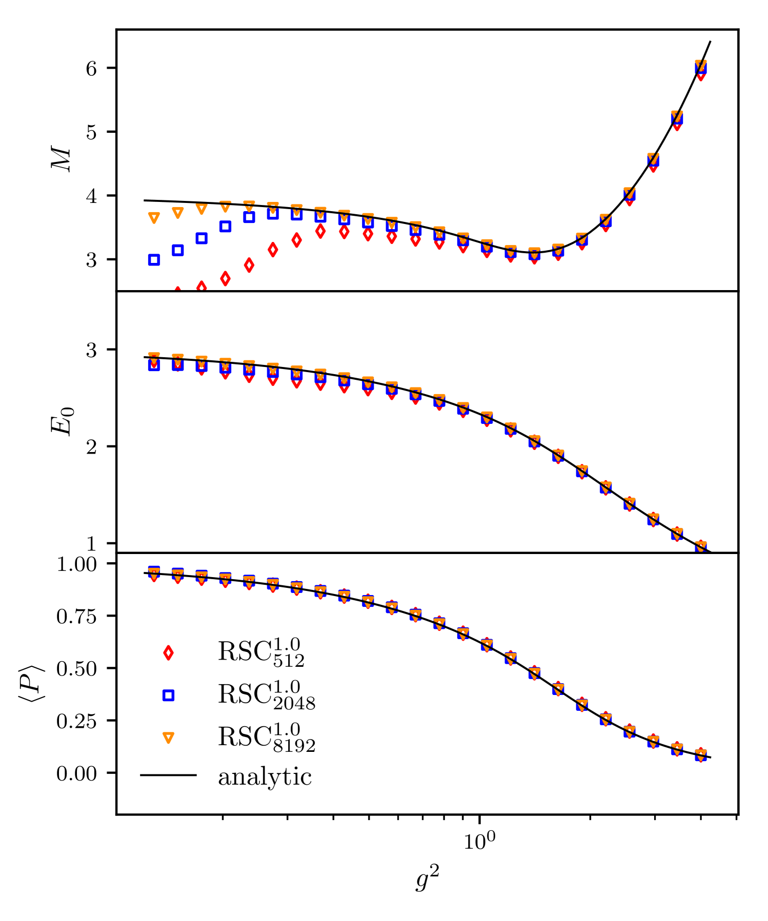
(a) Gauss law implemented via manual state selection.

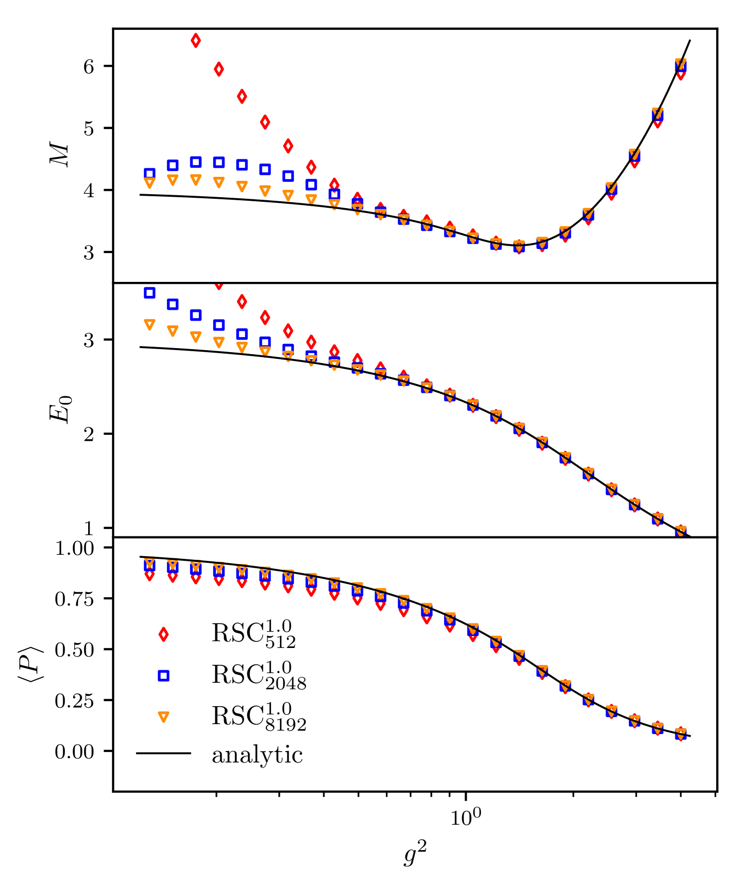
(b) Gauss law implemented via penalty term with $\kappa=5$.

Figure 3: Shown are the mass gap $M$, the ground state energy $E_{0}$ and the ground state plaquette expectation value $\langle P\rangle$ (as defined in eq. 38) as a function of the coupling $g^{2}$ for three different partitioning sizes. On the left physical states are selected manually while on the right a penalty term is used. The solid line shows the analytic prediction of each observable.

In fig. 3 we show all three observables as a function of the squared coupling $g^{2}$. For fig. 3(a), physical states were selected manually – which is possible since the analytic solution is known, while in fig. 3(b) the penalty term with $\kappa=5$ was used. The data points are obtained for partitionings with $256$ (red diamonds), $1024$ (blue squares) and $4096$ (orange triangles) elements and cover the whole gauge group without truncation (corresponding to $\varepsilon_{\mathrm{Tr}}=1$).

At larger values of the coupling, we see good agreement of all observables with the corresponding analytic prediction represented by the black, continuous lines. Towards smaller couplings, however, the simulation results increasingly deviate. As expected, these deviations are biggest for the coarse partitioning and decrease when going to finer partitionings.

Curiously, the amount and sign of the deviation changes, depending on whether physical states are selected manually or via the penalty term. For the former the mass gap and ground state energy are underestimated towards small $g^{2}$. The penalty term however, leads to an overestimation of the ground state energy and mass gap, while the plaquette expectation value is notably smaller than predicted. Note that the energies as plotted are already corrected for the penalty term expectation value as described in eq. 40.

To explain this we can take a look at the plaquette expectation value. For the manual state selection the analytic prediction is matched well, even for very small $g^{2}$. This suggests, that the correct states are still found, but their electric energy is underestimated by the meshed operators.

When using the penalty term however, the measured plaquette expectation values are found to be smaller than the prediction. This is likely because states with a large plaquette expectation value have more electrical energy and thus also lead to larger discretisation errors in the penalty term.

Lastly we note, that deviations appear to be largest in the mass gap. Thus, we will focus on this observable for our remaining tests.

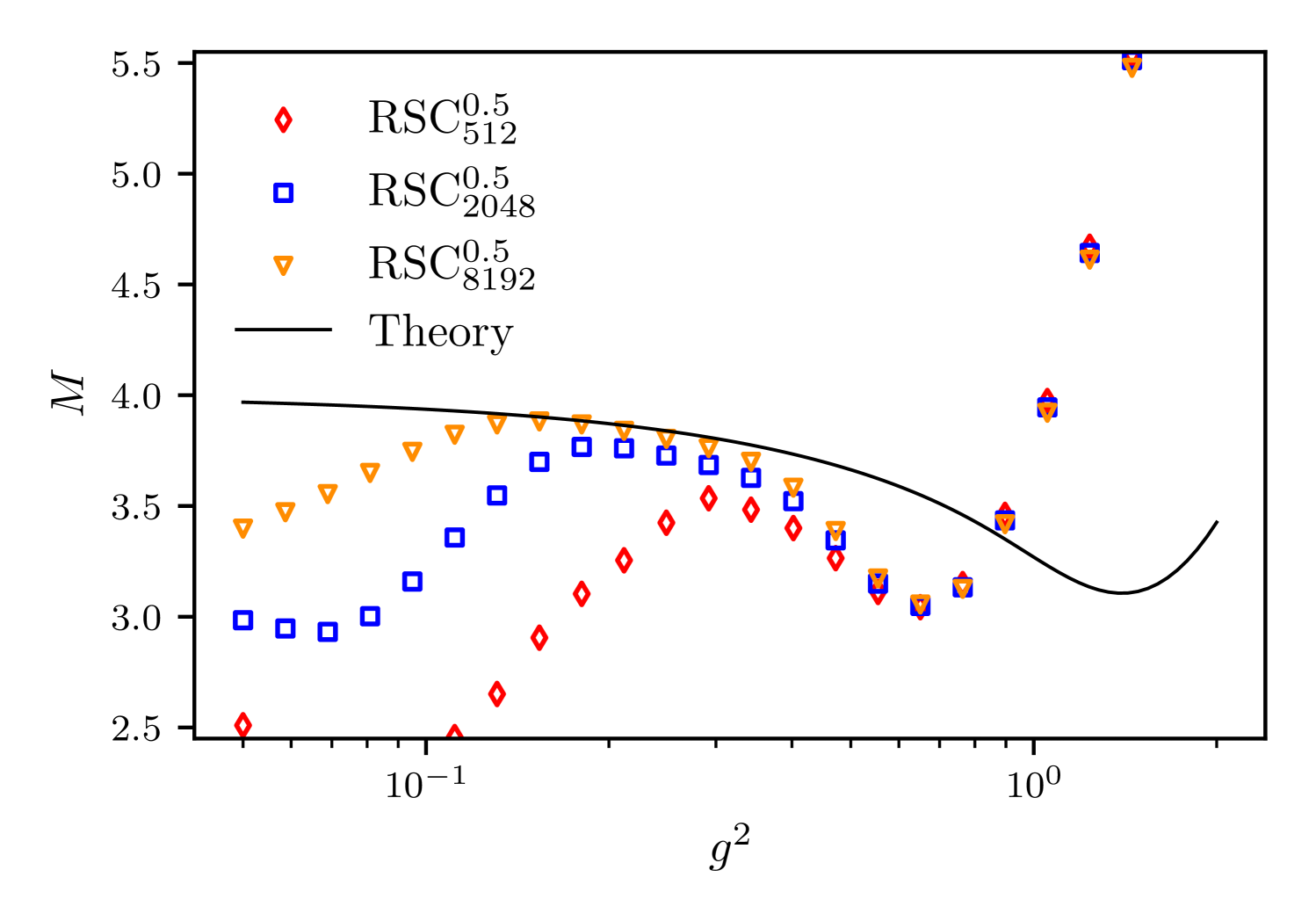
Figure 4: Plotted is the mass gap $M$ as a function of the coupling $g^{2}$ for three partitioning sizes with $\varepsilon_{\mathrm{Tr}}=0.5$. The analytic prediction is again shown in black.

IV.3 Truncation

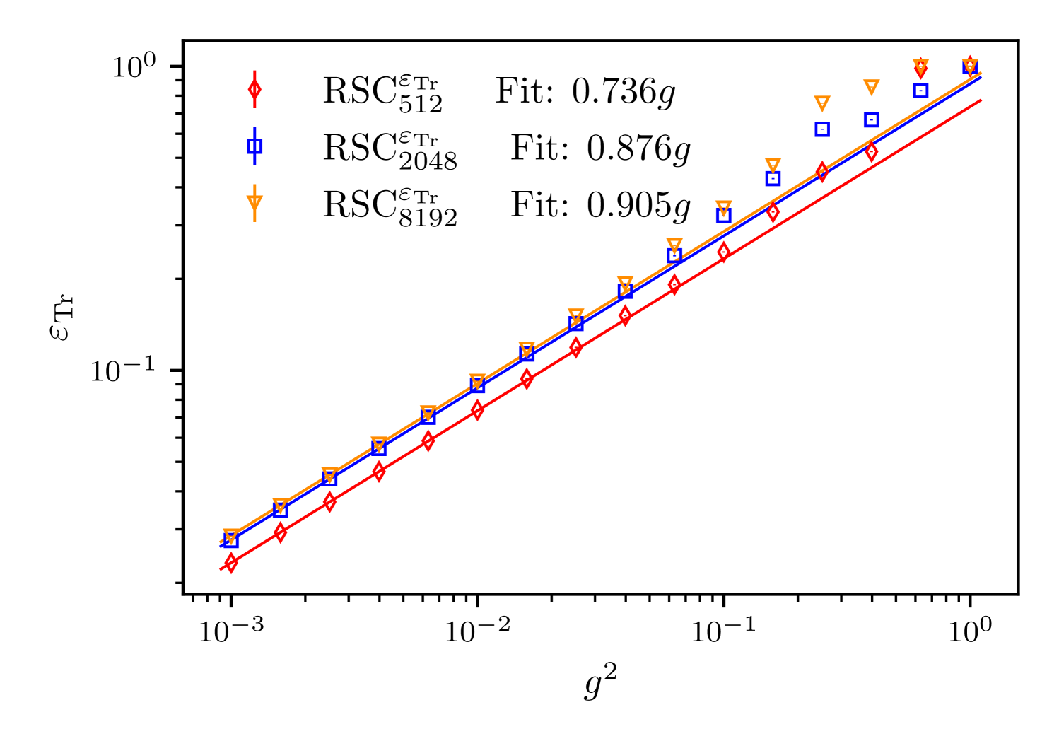
Figure 5: Plotted are the optimal values for $\varepsilon_{\mathrm{Tr}}$ as a function of the coupling for three different partitionings. The optimal value is found by minimizing the deviation from the analytic prediction of the mass gap. The error bars show the resolution of the scan used to find this minimum. Also shown are fits to 5 leftmost points in the plot.

Next we would like to test partitionings with $\varepsilon_{\mathrm{Tr}}<1$. We expect an interval $I$ in $g^{2}$ where the approximation works best: At large $g^{2}$-values errors due to too small $\varepsilon_{\mathrm{Tr}}$ will dominate, while at small values of $g^{2}$, the resolution around the identity is insufficient.

Moreover, increasing the resolution of the partitioning at fixed $\varepsilon_{\mathrm{Tr}}$ should move this interval to smaller values of $g^{2}$ and decrease the overall deviation in this interval region to the exact result.

This expectation is confirmed by our simulations. As an example we show in fig. 4 the mass gap as a function of the coupling for three different partitioning sizes with $\varepsilon_{\mathrm{Tr}}=0.5$. As predicted there is a matching interval at $g^{2}\approx 0.2$, which increases in size and moves to smaller couplings with finer partitionings.

In practice, this means one would rather choose $\varepsilon_{\mathrm{Tr}}$ too large than to small, as the former will still recover the correct result in the limit of infinitely fine partitionings, be it at higher cost.

In order to determine an appropriate truncation for a given coupling, we determined $\varepsilon_{\mathrm{Tr}}^{\mathrm{opt}}$ such that the deviation from the analytic prediction of the mass gap is minimized. The results can be found in fig. 5, where the such determined $\varepsilon_{\mathrm{Tr}}^{\mathrm{opt}}$ is plotted as a function of $g^{2}$, again for three different partitioning sizes. For about $g^{2}<0.1$ the dependence is to a good approximation linear in $g$. This is in agreement with the results in Ref. D’Andrea et al. (2024). $\varepsilon_{\mathrm{Tr}}^{\mathrm{opt}}$ also increases with partitioning size. This is the same effect mentioned earlier: the matching interval moves to smaller coupling values with increasing partitioning size at fixed $\varepsilon_{\mathrm{Tr}}^{\mathrm{opt}}$.

To predict the optimal truncation for a given coupling, we performed linear fits in $g$ to the data. As we are most interested in small couplings, only the five leftmost points in the plot were used for the fit. The truncation parameters derived from these fits will be referred to as $\varepsilon_{\mathrm{opt}}$ in the following.

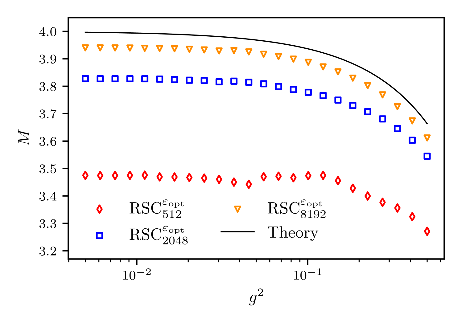
Figure 6: The mass gap $M$ as a function of the coupling $g^{2}$ for different fixed partitioning sizes. $\varepsilon_{\mathrm{Tr}}$ is chosen separately at each coupling according the fits found in fig. 5.

Finally, in fig. 6 we show the mass gap $M$ as a function of $g^{2}$, again for three resolutions simulated with the corresponding $\varepsilon_{\mathrm{Tr}}^{\mathrm{opt}}(g^{2})$ and compared to the analytical results. The finer the resolution, the smaller the deviation from the analytical curve at each $g^{2}$-value. And, the deviation for each partitioning size appears to become independent of $g^{2}$ in the $g\to 0$ limit.

IV.4 Convergence and Cost

To get a more quantitative idea of this and the accuracy of the partitionings, we study the relative deviation

$$\delta M=\frac{\left|M-M_{\mathrm{analytic}}\right|}{M_{\mathrm{analytic}}}\,.$$ (41)

$\delta M$ is plotted as a function of $g^{2}$ in fig. 7. There one can observe more clearly that the deviations are mostly independent of the coupling for $g^{2}\to 0$, which means the weak coupling limit can be approached at approximately constant simulation cost and uncertainty.

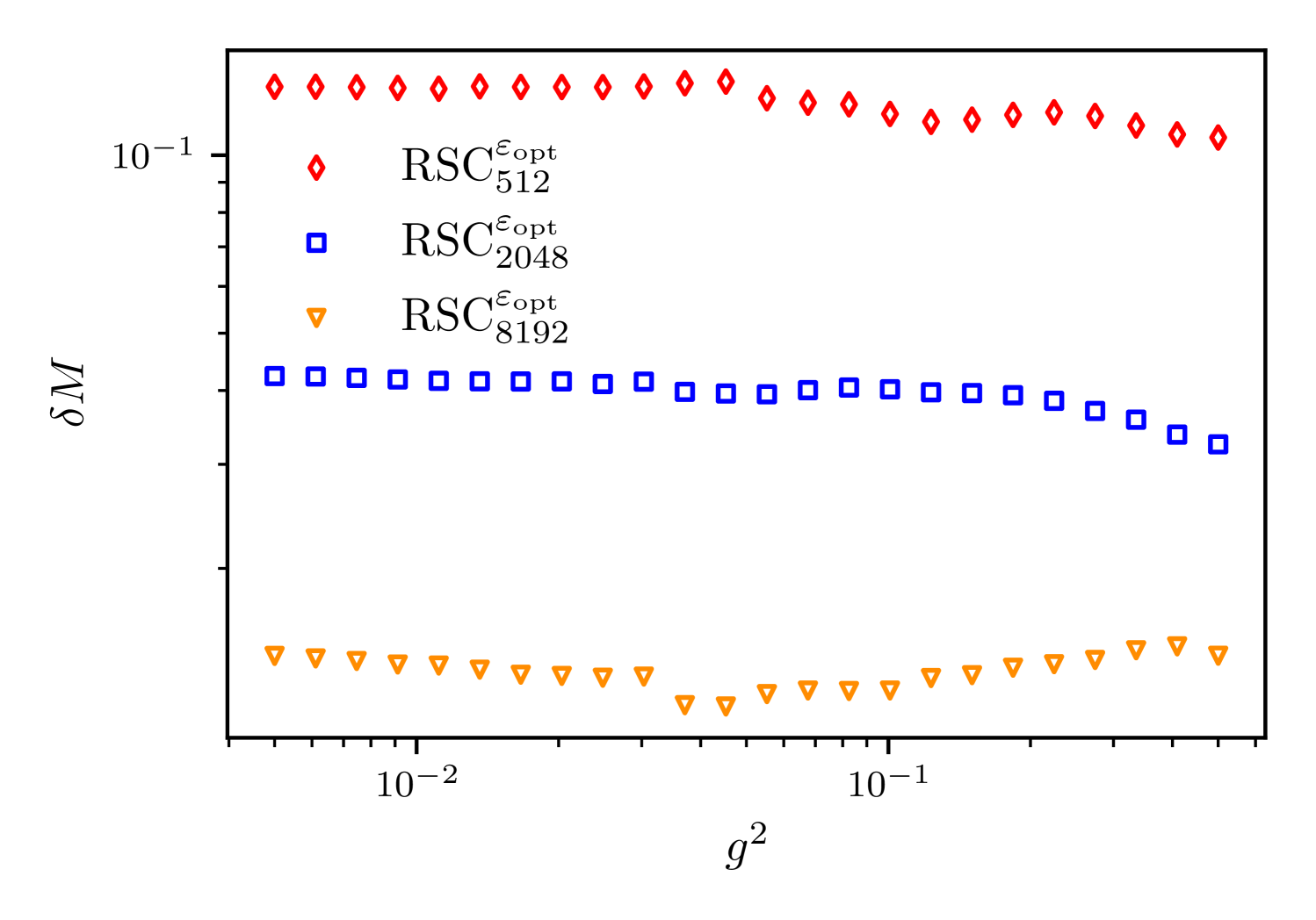
Figure 7: The relative deviation $\delta M$ of the mass gap shown in fig. 6 as a function of $g^{2}$ at fixed partitioning sizes.

Next, we plot the relative deviation as a function of the inverse partitioning size in fig. 8 at $g^{2}=0.01$. Here, the red diamonds are obtained by manual selection of the physical states from the Hamiltonian, while the blue points are obtained using the penalty term with $\kappa=5$. The results obtained with the penalty term show larger deviations, but both approaches seem to have a similar convergence rate. While selecting the physical state manually seems to produce more accurate results, it becomes quickly unfeasible when the system size increases.

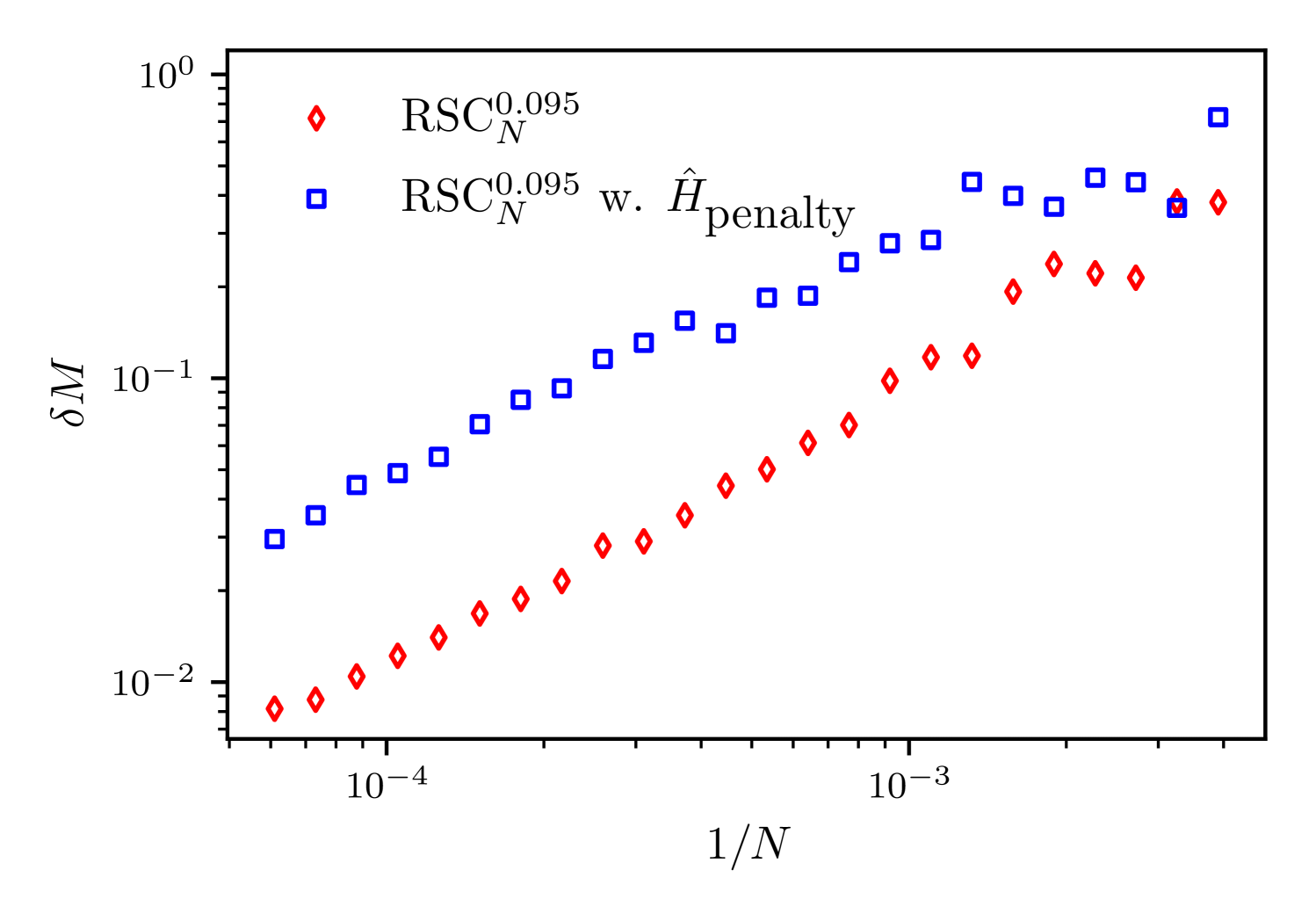
Figure 8: The relative deviation of the mass gap $\delta M$ as a function of the inverse partitioning size $1/N$ at a coupling of $g^{2}=0.01$ and $\varepsilon_{\mathrm{Tr}}=0.92g$. Results are obtained with penalty term (blue) and without (red).

IV.5 Extrapolating to the Full Group

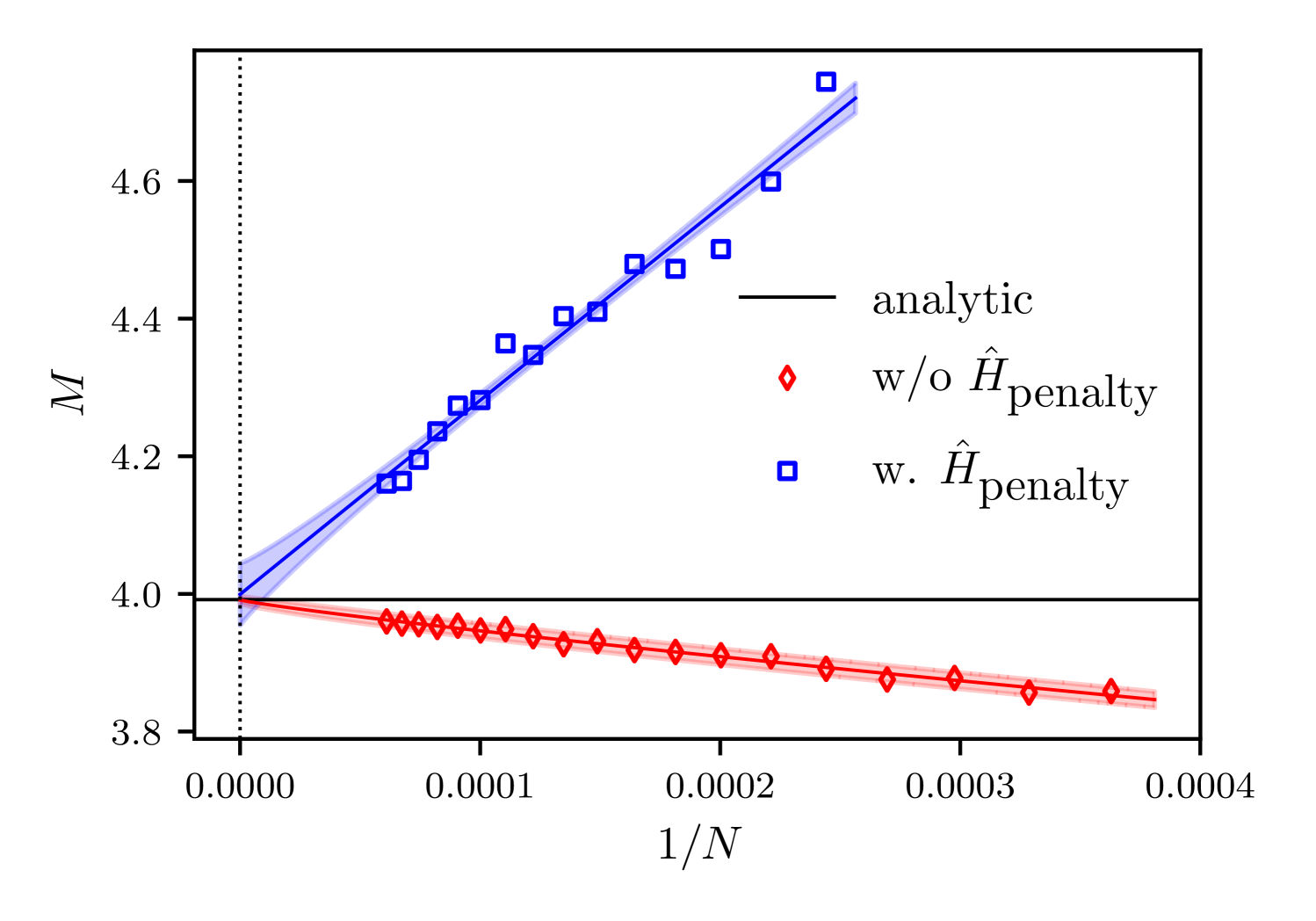
(a) Plotted is the mass gap $M$ as a function of the inverse partitioning size at a coupling of $g^{2}=0.01341$. Results are obtained with penalty term (blue) and without (red). In black, we plot the analytic solution. Also included are fits according to eq. 42. These allow us to extrapolate to $N\to\infty$.

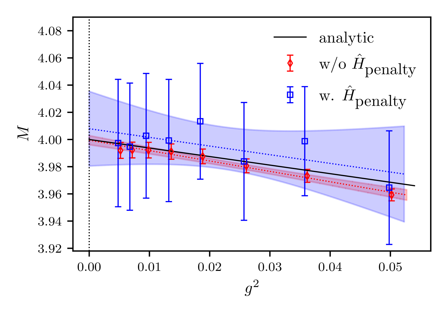
(b) Plotted is the mass gap in the limit $N\to\infty$ as a function of the coupling $g^{2}$. The data is obtained from fits like the one shown on the left. The analytic solution is again plotted in black. Also included are linear fits to the data. These allow us to extrapolate to $g^{2}\to 0$.

Figure 9: These two figures contain extrapolations for the mass gap $M$ first in the limit of $N\to\infty$ (left) and then $g^{2}\to 0$ (right). This is done to determine the mass gap one would expect for the full gauge group in the continuum limit. The truncation parameter is chosen to be $\varepsilon_{\mathrm{Tr}}=1.1g$ when the penalty term is used, and $\varepsilon_{\mathrm{Tr}}=0.95g$ without.

Lastly, we would like to test whether we can successfully extrapolate first to the full gauge group and then to $g^{2}=0$. To do so we collect data at eight different couplings $0.005\leq g^{2}\leq 0.05$ and partitioning sizes up to $N=2^{14}=16\,384$. When using the penalty term with $\kappa=5$, ${\varepsilon_{\mathrm{Tr}}=1.1g}$ was chosen, for the manual state selection ${\varepsilon_{\mathrm{Tr}}=0.95g}$. Choosing $\varepsilon$ a bit larger, when using the penalty term appears to improve results significantly, which at this point is a purely empirical observation.

In the first step we then perform a least squares fit to extrapolate to infinitely fine partitionings at fixed coupling. The Ansatz for the fit function reads

$$M_{g^{2}}(N)=M^{0}_{g^{2}}\pm\left(\frac{N^{0}_{g^{2}}}{N}\right)^{b}\,.$$ (42)

Here $M^{0}_{g^{2}}$ and $N^{0}_{g^{2}}$ are treated as separate parameters for each coupling, while the exponent $b$ is fitted globally to all eight datasets for different couplings. The sign is chosen positive for manual state selection and negative for the penalty term data.

This ansatz appears to describe the data well, while the global fit produces more stable results as compared to separate fits per $g$-value. As an example, we show the resulting fit for $g^{2}=0.01341$ together with the data in fig. 9(a). The (global) convergence rate is measured to be $b=1.00(11)$ with and $b=0.88(6)$ without the penalty term, respectively. The remaining best fit parameters can be found in table 1. Uncertainties are estimated from the inverse hessian, rescaled by the variance of the residuals. The analytically predicted result at this $g^{2}$-value is reproduced well in the limit $N\rightarrow\infty$, with and without penalty term.

Furthermore, the results of the extrapolations at all our $g^{2}$-values can be found in fig. 9(b). Here we also show linear fits of the expected weak coupling form

$$M(g^{2})=M_{0}+c\,g^{2}$$ (43)

to the data with and without penalty term. These allow us to extrapolate to $g^{2}=0$, i.e. take the weak coupling limit. Both of these fits agree within the estimated uncertainty with the analytic prediction plotted in black. At $g^{2}=0$ we get $M_{0}=4.008(27)$ with and $M_{0}=3.999(3)$ without the penalty term, both of which are compatible with $M_{0}=4$.

	w/o $\hat{H}_{\textrm{penalty}}$		w. $\hat{H}_{\textrm{penalty}}$
$g^{2}$	$M^{0}_{g^{2}}$	$N^{0}_{g^{2}}$	$M^{0}_{g^{2}}$	$N^{0}_{g^{2}}$
$0.0050$	$3.992(6)$	$3.0(4)\times 10^{2}$	$4.00(5)$	$2.97(16)\times 10^{3}$
$0.0069$	$3.992(6)$	$3.0(4)\times 10^{2}$	$3.99(5)$	$2.96(16)\times 10^{3}$
$0.0097$	$3.992(6)$	$3.0(4)\times 10^{2}$	$4.00(5)$	$2.88(15)\times 10^{3}$
$0.0134$	$3.991(6)$	$2.9(4)\times 10^{2}$	$4.00(4)$	$2.81(15)\times 10^{3}$
$0.0186$	$3.988(5)$	$2.7(4)\times 10^{2}$	$4.01(4)$	$2.61(15)\times 10^{3}$
$0.0259$	$3.981(5)$	$2.5(4)\times 10^{2}$	$3.98(4)$	$2.67(15)\times 10^{3}$
$0.0360$	$3.973(5)$	$2.2(4)\times 10^{2}$	$4.00(4)$	$2.41(15)\times 10^{3}$
$0.0500$	$3.959(4)$	$1.9(3)\times 10^{2}$	$3.96(4)$	$2.55(15)\times 10^{3}$

Table 1: Fit parameters according to eq. 42 for the extrapolation to the full gauge group at the eight different couplings.

V Discussion

A few of our observations deserve further discussion. The newly constructed $\hat{Q}^{2}$ operator, needed for the Gauss law penalty term, seems to work well. The deviations from the analytic prediction increase, but the convergence rate seems to be unchanged. It is likely that this effect can be further reduced by tuning $\kappa$, the prefactor of the penalty term, more carefully. Penalty terms constructed from the dual Gauss laws found in Ref. D’Andrea et al. (2024) and Ref. Mathur and Rathor (2023) would also both contain this operator. The fact, that it can be used in simulations without major complications is thus quite reassuring.

Furthermore, considering partitionings with points only distributed in the vicinity of $\mathbb{1}$ seems to be a valid strategy to approach the weak coupling limit. When tuning the truncation parameter $\varepsilon_{\mathrm{Tr}}$ appropriately, the relative deviations of the mass gap were shown to be largely independent of the coupling at fixed operator dimension. Similar to the approach presented in Ref. D’Andrea et al. (2024), we showed that the truncation parameter $\varepsilon_{\mathrm{Tr}}$ scales linearly with $g$ at small couplings.

Simulations using the penalty term typically were more reliable when slightly increasing $\varepsilon_{\mathrm{Tr}}$ compared to the simulations with manual state selection. This is likely because discretisation errors at the boundary of the truncation have more of an impact when filtering for physical states. Increasing the size of the sphere cap means that these effects are more suppressed. One possibility to address this in the future would be to test whether non-uniform partitionings can be used. Here one would aim for a high density of points around $\mathbb{1}$ and a decreasing density in the rest of the group. This should in principle reduce boundary effects and might lead to more accurate simulations.

Another open question is the convergence rate of the observables. Reliable extrapolations for $N\to\infty$ were only possible when including the exponent of convergence as a fit parameter. In our previous tests Jakobs et al. (2023a) we found a convergence rate of $N^{-2/3}$ for the spectrum of $\sum_{c}(\hat{L^{c}})^{2}$ which would be proportional to the lattice spacing squared in the partitioning. Here we observe rates of $N^{-0.88(6)}$ and $N^{-1.00(11)}$ depending on whether a penalty term to enforce Gauss law is used or not. Currently, we do not have an analytic prediction of these rates available.

Lastly, it should be mentioned that similar numerical tests have been conducted in Ref. D’Andrea et al. (2024). They propose a different discretisation scheme and achieve good matching with the analytic prediction at significantly smaller operator dimension.

VI Conclusion and Outlook

In this paper we have shown, that the digitised canonical momentum operators for the Hamiltonian formulation of an SU$(2)$ gauge theory, originally proposed in Ref. Jakobs et al. (2023a), represent an efficient choice for simulations at very weak couplings.

In this approach the Hilbert space is digitised by choosing a finite set of gauge group elements, called a partitioning. The canonical momentum operators are then approximated by finite element methods. While these operators break the fundamental commutation relations of the theory, they are local in the gauge group. We have shown here how to define a penalty term based on the squared Gauss operator approximated again using finite element methods to project to physical states of the system. Given a suitable dual formulation of the Kogut-Susskind Hamiltonian with a local magnetic term, one can thus use partitionings with points distributed only around the identity. We show numerically that this ansatz allows us to approach the weak coupling limit at constant operator dimensions for a single plaquette system.

For this we first study how to truncate these partitionings at a given coupling $g^{2}$. We showed, that the cut-off parameter $\varepsilon_{\mathrm{Tr}}$ as defined in eq. 36 scales linearly with $g$, in agreement with results from Ref. D’Andrea et al. (2024). By choosing $\varepsilon_{\mathrm{Tr}}$ optimally for each coupling value, we then numerically show that the relative deviations of the mass gap of the theory are independent of the coupling value.

Lastly we have demonstrated that the correct mass gap of the theory is recovered, when extrapolating first to infinitely fine partitionings and then to $g^{2}\to 0$. This leaves us hopeful that these operators might find use for the simulation of larger systems at very weak couplings in the future. However, other approaches like e.g. the one from Ref. D’Andrea et al. (2024) achieve the same, but currently appear to be more resource efficient for the system investigated here. In general though, it is still unclear which approach of the many available on the market will be most suitable for the simulation of larger systems with three spatial dimensions and SU$(3)$ as the gauge group.

References

- Kogut and Susskind (1975) John B. Kogut and Leonard Susskind, “Hamiltonian Formulation of Wilson’s Lattice Gauge Theories,” Phys. Rev. D 11, 395–408 (1975).
- Zohar and Burrello (2015) Erez Zohar and Michele Burrello, “Formulation of lattice gauge theories for quantum simulations,” Phys. Rev. D 91, 054506 (2015), arXiv:1409.3085 [quant-ph] .
- Grabowska et al. (2024) Dorota M. Grabowska, Christopher F. Kane, and Christian W. Bauer, “A Fully Gauge-Fixed SU(2) Hamiltonian for Quantum Simulations,” (2024), arXiv:2409.10610 [quant-ph] .
- D’Andrea et al. (2024) Irian D’Andrea, Christian W. Bauer, Dorota M. Grabowska, and Marat Freytsis, “New basis for Hamiltonian SU(2) simulations,” Phys. Rev. D 109, 074501 (2024), arXiv:2307.11829 [hep-ph] .
- Gustafson et al. (2022) Erik J. Gustafson, Henry Lamm, Felicity Lovelace, and Damian Musk, “Primitive quantum gates for an SU(2) discrete subgroup: Binary tetrahedral,” Phys. Rev. D 106, 114501 (2022), arXiv:2208.12309 [quant-ph] .
- Gustafson et al. (2024) Erik J. Gustafson, Henry Lamm, and Felicity Lovelace, “Primitive quantum gates for an SU(2) discrete subgroup: Binary octahedral,” Phys. Rev. D 109, 054503 (2024), arXiv:2312.10285 [hep-lat] .
- Burbano and Bauer (2024) I. M. Burbano and Christian W. Bauer, “Gauge Loop-String-Hadron Formulation on General Graphs and Applications to Fully Gauge Fixed Hamiltonian Lattice Gauge Theory,” (2024), arXiv:2409.13812 [hep-lat] .
- Ji et al. (2020) Yao Ji, Henry Lamm, and Shuchen Zhu (NuQS), “Gluon Field Digitization via Group Space Decimation for Quantum Computers,” Phys. Rev. D 102, 114513 (2020), arXiv:2005.14221 [hep-lat] .
- Alexandru et al. (2019) Andrei Alexandru, Paulo F. Bedaque, Siddhartha Harmalkar, Henry Lamm, Scott Lawrence, and Neill C. Warrington (NuQS), “Gluon Field Digitization for Quantum Computers,” Phys. Rev. D 100, 114501 (2019), arXiv:1906.11213 [hep-lat] .
- Alexandru et al. (2022) Andrei Alexandru, Paulo F. Bedaque, Ruairí Brett, and Henry Lamm, “Spectrum of digitized QCD: Glueballs in a S(1080) gauge theory,” Phys. Rev. D 105, 114508 (2022), arXiv:2112.08482 [hep-lat] .
- Ji et al. (2023) Yao Ji, Henry Lamm, and Shuchen Zhu (NuQS), “Gluon digitization via character expansion for quantum computers,” Phys. Rev. D 107, 114503 (2023), arXiv:2203.02330 [hep-lat] .
- Chandrasekharan and Wiese (1997) S. Chandrasekharan and U. J. Wiese, “Quantum link models: A Discrete approach to gauge theories,” Nucl. Phys. B 492, 455–474 (1997), arXiv:hep-lat/9609042 .
- Brower et al. (1999) R. Brower, S. Chandrasekharan, and U. J. Wiese, “QCD as a quantum link model,” Phys. Rev. D 60, 094502 (1999), arXiv:hep-th/9704106 .
- Wiese (2021) Uwe-Jens Wiese, “From quantum link models to D-theory: a resource efficient framework for the quantum simulation and computation of gauge theories,” Phil. Trans. A. Math. Phys. Eng. Sci. 380, 20210068 (2021), arXiv:2107.09335 [hep-lat] .
- Bhattacharya et al. (2021) Tanmoy Bhattacharya, Alexander J. Buser, Shailesh Chandrasekharan, Rajan Gupta, and Hersh Singh, “Qubit regularization of asymptotic freedom,” Phys. Rev. Lett. 126, 172001 (2021), arXiv:2012.02153 [hep-lat] .
- Bergner et al. (2024) Georg Bergner, Masanori Hanada, Enrico Rinaldi, and Andreas Schäfer, “Toward qcd on quantum computer: orbifold lattice approach,” Journal of High Energy Physics 2024, 234 (2024).
- Jakobs et al. (2023a) Timo Jakobs, Marco Garofalo, Tobias Hartung, Karl Jansen, Johann Ostmeyer, Dominik Rolfes, Simone Romiti, and Carsten Urbach, “Canonical momenta in digitized SU(2) lattice gauge theory: definition and free theory,” Eur. Phys. J. C 83, 669 (2023a), arXiv:2304.02322 [hep-lat] .
- Hartung et al. (2022) Tobias Hartung, Timo Jakobs, Karl Jansen, Johann Ostmeyer, and Carsten Urbach, “Digitising SU(2) gauge fields and the freezing transition,” Eur. Phys. J. C 82, 237 (2022), arXiv:2201.09625 [hep-lat] .
- Jakobs et al. (2023b) Timo Jakobs, Tobias Hartung, Karl Jansen, Johann Ostmeyer, and Carsten Urbach, “Digitizing SU(2) gauge fields and what to look out for when doing so,” PoS LATTICE2022, 015 (2023b), arXiv:2212.09496 [hep-lat] .
- Garofalo et al. (2024) Marco Garofalo, Tobias Hartung, Timo Jakobs, Karl Jansen, Johann Ostmeyer, Dominik Rolfes, Simone Romiti, and Carsten Urbach, “Testing the lattice Hamiltonian built from partitionings,” PoS LATTICE2023, 231 (2024), arXiv:2311.15926 [hep-lat] .
- Romiti and Urbach (2024) Simone Romiti and Carsten Urbach, “Digitizing lattice gauge theories in the magnetic basis: reducing the breaking of the fundamental commutation relations,” Eur. Phys. J. C 84, 708 (2024), arXiv:2311.11928 [hep-lat] .
- Wilson (1974) Kenneth G. Wilson, “Confinement of Quarks,” Phys. Rev. D 10, 2445–2459 (1974).
- Ligterink et al. (2000a) N.E. Ligterink, N.R. Walet, and R.F. Bishop, “Toward a Many-Body Treatment of Hamiltonian Lattice SU(N) Gauge Theory,” Annals of Physics 284, 215–262 (2000a).
- Mathur and Rathor (2023) Manu Mathur and Atul Rathor, “Exact duality and local dynamics in SU(N) lattice gauge theory,” Phys. Rev. D 107, 074504 (2023).
- Halimeh and Hauke (2020) Jad C. Halimeh and Philipp Hauke, “Reliability of lattice gauge theories,” Phys. Rev. Lett. 125, 030503 (2020).
- Delaunay (1934) B. N. Delaunay, “Sur la sphère vide,” Bulletin of Academy of Sciences of the USSR 7, 793–800 (1934).
- Ligterink et al. (2000b) N. E. Ligterink, N. R. Walet, and R. F. Bishop, “Towards a many body treatment of Hamiltonian lattice SU(N) gauge theory,” Annals Phys. 284, 215–262 (2000b), arXiv:hep-lat/0001028 .