Some contributions on Melnikov chaos for smooth and piecewise-smooth planar systems: “trajectories chaotic in the future”

Abstract

We consider a $2$-dimensional autonomous system subject to a $1$-periodic perturbation, i.e.

$$\dot{\vec{x}}=\vec{f}(\vec{x})+\varepsilon\vec{g}(t,\vec{x},\varepsilon),\quad\vec{x}\in\Omega.$$

We assume that for $\varepsilon=0$ there is a trajectory $\vec{\gamma}(t)$ homoclinic to the origin which is a critical point: in this context Melnikov theory provides a sufficient condition for the insurgence of a chaotic pattern when $\varepsilon\neq 0$.

In this paper we show that for any line $\Xi$ transversal to $\{\vec{\gamma}(t)\mid t\in{\mathbb{R}}\}$ and any $\tau\in[0,1]$ we can find a set $\Sigma^{+}(\Xi,\tau)$ of initial conditions giving rise to a pattern chaotic just in the future, located in $\Xi$ at $t=\tau$. Further diam$(\Sigma^{+}(\Xi,\tau))\leq\varepsilon^{(1+\nu)/\underline{\sigma}}$ where $\underline{\sigma}>0$ is a constant and $\nu>0$ is a parameter that can be chosen as large as we wish.

The same result holds true for the set $\Sigma^{-}(\Xi,\tau)$ of initial conditions giving rise to a pattern chaotic just in the past. In fact all the results are developed in a piecewise-smooth context, assuming that $\vec{0}$ lies on the discontinuity curve $\Omega^{0}$: we recall that in this setting chaos is not possible if we have sliding phenomena close to the origin. This paper can also be considered as the first part of the project to show the existence of classical chaotic phenomena when sliding close to the origin is not present.

Keywords: Melnikov theory, piecewise-smooth systems, homoclinic trajectories, non-autonomous dynamical systems, non-autonomous perturbation

2020 AMS Subject Classification: Primary 34A36, 37G20, 37G30; Secondary 34C37, 34E10, 37C60.

1 Introduction

In this paper we study a $2$-dimensional piecewise-smooth system (possibly discontinuous), subject to a non-autonomous perturbation. Let us start for illustrative purposes to consider the smooth case, i.e.

$$\dot{\vec{x}}=\vec{f}(\vec{x})+\varepsilon\vec{g}(t,\vec{x},\varepsilon),\quad\vec{x}\in\Omega,$$ (S)

where $\Omega\subset{\mathbb{R}}^{2}$ is an open set, $\varepsilon\in{\mathbb{R}}$ is a small parameter, $\vec{f}$ and $\vec{g}$ are $C^{r}$, $r\geq 2$.

We assume that the origin $\vec{0}\in\Omega\subset{\mathbb{R}}^{2}$ is a critical point for (S) for any $\varepsilon\geq 0$ and that for $\varepsilon=0$ there is a trajectory $\vec{\gamma}(t)$ homoclinic to $\vec{0}$. The classical Melnikov theory provides a condition which is sufficient for the insurgence of a chaotic pattern for $\varepsilon\neq 0$. Namely it is sufficient to require that $\vec{g}$ is $1$-periodic in $t$ and that a computable function ${\mathcal{M}}(\tau)$, see (3.3) below, has a non-degenerate zero.

More precisely, let $\vec{x}(t,\tau;\vec{\xi})$ denote the trajectory leaving from $\vec{\xi}$ at $t=\tau$, and denote by $\Phi(t;\tau)\vec{\xi}=\vec{x}(t,\tau;\vec{\xi})$, so that $\Phi(t;\tau)$ is a $C^{r}$ diffemorphism for any $t,\tau\in{\mathbb{R}}$; let $\tau_{0}\in[0,1]$ be such that ${\mathcal{M}}(\tau_{0})=0\neq{\mathcal{M}}^{\prime}(\tau_{0})$. Let ${\boldsymbol{\Gamma}}=\{\vec{\gamma}(t)\mid t\in{\mathbb{R}}\}\cup\{\vec{0}\}$. Then, there is $\Theta(\varepsilon)$ large enough so that for any positive integer $k>\Theta(\varepsilon)$ we can find a set $\Sigma$ which is invariant for $\Phi(k+\tau_{0},\tau_{0})$ and which has the following properties. For any sequence ${\mathrm{e}}\in{\mathcal{E}}=\{0,1\}^{{\mathbb{Z}}}$ there is a unique $\vec{\xi}\in\Sigma$ such that the trajectory $\vec{x}(t,\tau_{0};\vec{\xi})$ is either “close to ${\boldsymbol{\Gamma}}$” or “close to the origin”; i.e., either $\|\vec{x}(t,\tau_{0};\vec{\xi})-\vec{\gamma}(t-T_{2j})\|=O(\varepsilon)$ or $\|\vec{x}(t,\tau_{0};\vec{\xi})\|=O(\varepsilon)$ whenever $t\in[T_{2j-1},T_{2j+1}]$, where $T_{j}=jk+\tau_{0}$.

This kind of results started from the work of Melnikov [27], but an important step forward was performed by Chow et al. in [10], and a big progress is due to [29] where Palmer addressed the $n$-dimensional case where $n\geq 2$. This theory has been generalized in several directions, in particular it has been extended to the almost periodic case, see e.g. [33, 31], and to the case where the zeros of ${\mathcal{M}}(\tau)$ are degenerate, see e.g. [1, 2]. Afterwards the so-called perturbation approach has been widely developed by many authors. Melnikov theory is by now well-established for smooth systems, and there are many works devoted to it. For example we refer to [10, 14, 16, 29, 30, 31, 33, 34, 28, 35, 36].

In this paper we review completely the construction of the chaotic pattern, motivated by the project to extend the classical theory to a discontinuous setting, and to relax further the assumptions on the recurrence properties and on non-degeneracy of the zeros of the Melnikov function. In particular all the proofs are written directly in the piecewise-smooth discontinuous setting.

However, in this paper we present some results of intrinsic mathematical interest, which, as far as we are aware, are new even in the smooth case. In particular we develop a new iterative scheme which allows us to select sets $\Sigma^{+}$ and $\Sigma^{-}$ giving rise to solutions performing a possibly infinite number of loops either in the future or in the past, following any prescribed sequence of two symbols. Roughly speaking the trajectories leaving from $\Sigma^{+}$ are “chaotic in the future”, while the ones leaving from $\Sigma^{-}$ are “chaotic in the past”: we find some information concerning $\Sigma^{\pm}$ which have not appeared previously in literature, as far as we are aware. More precisely let us consider, as before, the case in which $\vec{g}$ is $1$-periodic in $t$. Let $\Xi$ be a line (or more generally, any curve) transversal to any point in ${\boldsymbol{\Gamma}}\setminus\{\vec{0}\}$, say $\vec{\gamma}(s)$, $s\in{\mathbb{R}}$ for definiteness, let $\tau_{0}\in[0,1]$ and let $T_{j}=kj+\tau_{0}$ as above and set ${\mathcal{T}}^{+}=(T_{j})$, $j\geq 1$, ${\mathcal{T}}^{-}=(T_{j})$, $j\leq-1$. Then we construct the sets $\Sigma^{+}=\Sigma^{+}(\tau,{\mathcal{T}}^{+},\Xi)$ and $\Sigma^{-}=\Sigma^{-}(\tau,{\mathcal{T}}^{-},\Xi)$ with the following properties: if $\vec{\xi}\in\Sigma^{+}$ then $\vec{x}(t,\tau;\vec{\xi})$ is either “close to ${\boldsymbol{\Gamma}}$” or “close to the origin” for $t\geq\tau$, while if $\vec{\xi}\in\Sigma^{-}$, $\vec{x}(t,\tau;\vec{\xi})$ has this property for $t\leq\tau$ (see Section 3 for more details).

In fact we may also get a better localization: if we replace the constant $\Theta(\varepsilon)$ defined above by $(\nu+1)\Theta(\varepsilon)$ where $\nu\geq\nu_{0}\geq 1$ is arbitrary high, the set $\Sigma^{+}$ gets smaller. More precisely, let us denote by diam$(\Sigma^{+})$ the diameter of $\Sigma^{+}$. Then we get

$$\textrm{diam}(\Sigma^{+}):=\sup\{\|\vec{P}-\vec{Q}\|\mid\vec{P},\vec{Q}\in\Sigma^{+}\}=O(\varepsilon^{(1+\nu)/\underline{\sigma}}),$$

where $0<\underline{\sigma}<1$ is a constant which depends only on the eigenvalues of ${\boldsymbol{f_{x}}}(\vec{0})$, see (3.1). Whence $\textrm{diam}(\Sigma^{+})$ can be chosen arbitrarily small, even with respect to $\varepsilon$ which is the size of the perturbation, just paying the prize of a larger time spent by the trajectories to perform a loop; further $\Sigma^{+}$ is located in a one-dimensional set.

However, $\Sigma^{+}$ oscillates with $\tau$ within an $\varepsilon$-neighborhood of $\vec{\gamma}(s)$; so even if we know that its diameter is $O(\varepsilon^{(1+\nu)/\underline{\sigma}})$, and that it is $O(\varepsilon^{(1+\nu)/\underline{\sigma}})$ close to $\vec{P}_{s}(\tau)$, the intersection point between the stable manifold $\tilde{W}^{s}(\tau)$ and $\Xi$, we know its position just with $O(\varepsilon)$ accuracy.

In fact we have all the analogous results for the set $\Sigma^{-}$ giving rise to patterns chaotic in past.

As we will see in a forthcoming paper this $O(\varepsilon^{(1+\nu)/\underline{\sigma}})$ precision on the size of $\Sigma^{+}$ and $\Sigma^{-}$ is lost when we look at the set of initial conditions $\Sigma$ giving rise to the classical pattern: chaotic both in the past and in the future. In fact $\Sigma$ will lie $O(\varepsilon^{(1+\nu)/\underline{\sigma}})$ close to the stable and unstable manifold but it will spread in an $O(\varepsilon)$ neighborhood along the direction of ${\boldsymbol{\Gamma}}$. So we cannot locate $\Sigma$ in a one-dimensional set.

On the contrary, we emphasize once again that the sets $\Sigma^{\pm}$ are located in a $1$-dimensional object, $\Xi$, further we have a different set for any $\tau\in[0,1]$ and any line (or more generally, any curve) $\Xi$. Indeed we conjecture that for any ${\mathrm{e}}^{+}\in{\mathcal{E}}^{+}$ and any $\tau\in[0,1]$ we may find a manifold of initial conditions of trajectories which mimic the sequence ${\mathrm{e}}^{+}$ in forward time.

Our approach, inspired by the work by Battelli and Fečkan, see [3, 4, 5, 6], allows us to obtain a great flexibility in the choice of the sets $\Sigma^{\pm}$, and to weaken the recurrence properties required from the Melnikov function ${\mathcal{M}}(\tau)$, see (3.3) below.
Let us consider again the smooth case. In fact, even if the system is $1$-periodic we can choose aperiodic sequences $\tilde{{\mathcal{T}}}=(\tilde{T}_{j})_{j\in{\mathbb{Z}}}$. For example we can choose $\tilde{{\mathcal{T}}}$ so that the gap $\tilde{T}_{j}-\tilde{T}_{j-1}$ varies periodically between $\big{[}\Theta+1\big{]}$ and $2\big{[}\Theta+1\big{]}$ (here $[\cdot]$ denotes the integer part) or it becomes unbounded. Further, if there is $\tau_{1}\neq\tau_{0}$ such that ${\mathcal{M}}(\tau_{1})=0\neq{\mathcal{M}}^{\prime}(\tau_{1})$ and $\tau_{1}\in[0,1]$, we may choose a sequence $\bar{{\mathcal{T}}}=(\bar{T}_{j})_{j\in{\mathbb{Z}}}$ jumping randomly from a translate of $\tau_{0}$ to a translate of $\tau_{1}$.

Anytime we change either one of $\tau$, ${\mathcal{T}}^{\pm}$ we obtain different sets $\Sigma^{\pm}$ (in fact infinitely many of them) giving rise to different chaotic patterns and they are all contained in the same $O(\varepsilon^{(1+\nu)/\underline{\sigma}})$ one-dimensional neighborhood, and they vary also if we change $\Xi$.

In our opinion all these results concerning $\Sigma^{+}$ and $\Sigma^{-}$ increase our knowledge on the sensitive dependence of the system on initial conditions.

We stress the fact that we assume much weaker recurrence properties than the classical ones. In particular we do not require any non-degeneracy of the zeros of ${\mathcal{M}}(\tau)$ (we just need ${\mathcal{M}}$ to change sign): this allows us to consider systems in which $\vec{g}$ is made up by a sum of a periodic component and a noise, not necessarily small, and on which we have little information, see Remark 3.9.

Further we show that, in the periodic case, the action of $\Phi(T_{i+1},T_{i})$ on $\Sigma^{+}$ and $\Sigma^{-}$ is semi-conjugated to the action of the Bernoulli shift on ${\mathcal{E}}^{+}=\{0;1\}^{{\mathbb{Z}}^{+}}$ and ${\mathcal{E}}^{-}=\{0;1\}^{{\mathbb{Z}}^{-}}$ respectively, and we obtain analogous results in the aperiodic case.

In fact all the results of this paper are obtained already in a piecewise-smooth context. More precisely we consider the piecewise-smooth system

$$\dot{\vec{x}}=\vec{f}^{\pm}(\vec{x})+\varepsilon\vec{g}(t,\vec{x},\varepsilon),\quad\vec{x}\in\Omega^{\pm},$$ (PS)

where $\Omega^{\pm}=\{\vec{x}\in\Omega\mid\pm G(\vec{x})>0\}$, $\Omega^{0}=\{\vec{x}\in\Omega\mid G(\vec{x})=0\}$, $G$ is a $C^{r}$-function on $\Omega$ with $r>1$ such that $0$ is a regular value of $G$. Next, $\vec{f}^{\pm}\in C^{r}_{b}(\Omega^{\pm}\cup\Omega^{0},{\mathbb{R}}^{2})$, $\vec{g}\in C_{b}^{r}({\mathbb{R}}\times\Omega\times{\mathbb{R}},{\mathbb{R}}^{2})$ and $G\in C_{b}^{r}(\Omega,{\mathbb{R}})$, i.e., the derivatives of $\vec{f}^{\pm}$, $\vec{g}$ and $G$ are uniformly continuous and bounded up to the $r$-th order, respectively, if $r\in{\mathbb{N}}$ and up to $r_{0}$ if $r=r_{0}+r_{1}$, with $r_{0}\in{\mathbb{N}}$ and $0<r_{1}<1$ and the $r_{0}$-th derivatives are $r_{1}$ Hölder continuous.

In the last 20 years many authors addressed the problem of generalizing Melnikov theory to a discontinuous (piecewise-smooth) setting, but assuming that $\vec{0}\not\in\Omega^{0}$: among the other papers, let us mention e.g., [22, 23, 24, 3, 5, 8, 7, 11, 15, 21]. Most of the cited papers concern the $2$-dimensional case, but Battelli and Fečkan managed to address the $n\geq 2$ case, and they proved the persistence of homoclinic [3], the insurgence of chaos when the unperturbed homoclinic exhibits no sliding phenomena [5] and when it does [4].

If, instead, we assume that the critical point lies on the discontinuity hypersurface (in the case $n=2$, the curve $\Omega^{0}$), the problem of detecting a chaotic behavior becomes even more challenging. In this setting, as a preliminary step, in [8, 21, 18] it was shown that the Melnikov condition found by Battelli and Fečkan together with a further (generic) transversality requirement (always satisfied in two dimensions) are enough to prove the persistence of the homoclinic trajectory in the $n\geq 2$ case.

Quite surprisingly, in [12], which is still set in the two-dimensional case, it was shown that the Melnikov condition, which ensures the persistence of the homoclinic [8] and the transversality of the crossing between stable and unstable leaves, does not guarantee the insurgence of chaos differently from the smooth setting, and also from the piecewise-smooth setting considered, e.g., in [22, 23, 24, 3, 5, 8, 7, 25, 26]. In fact, a natural geometrical obstruction prevents the formation of chaotic patterns, and new bifurcation phenomena take place, scenarios which may exist just in a discontinuous context.

This paper can also be regarded as an intermediate step to complete the picture in the two-dimensional discontinuous case showing that, when this obstruction is removed, system (PS) exhibits a chaotic behavior as in the smooth setting: the complete result will appear in a forthcoming paper.

Summing up the main achievements of the paper are the following:

1

We construct new sets $\Sigma^{-}$ and $\Sigma^{+}$ of initial conditions giving rise respectively to patterns chaotic in the past and chaotic in the future. These sets lie on any arbitrarily chosen $1$-dimensional transversal to ${\boldsymbol{\Gamma}}\setminus\{\vec{0}\}$, say $\Xi$, and their diameters may be chosen of order $O(\varepsilon^{(1+\nu)/\underline{\sigma}})$, where $\nu\geq\nu_{0}\geq 1$ is arbitrary high and $\underline{\sigma}>0$ is a constant (independent of $\varepsilon$ and $\nu$), see (3.1), even if the size $\varepsilon$ of the perturbation is fixed. Further if we fix the sequence ${\mathcal{T}}^{\pm}$ we get a new $\Sigma^{\pm}$ whenever we let either $\tau$ or $\Xi$ vary.

2

We weaken the recurrence requirements on the function ${\mathcal{M}}(\tau)$ and we allow its zeros to be degenerate.

3

The results are proved in a piecewise-smooth setting, and they are a first step to prove the existence of a classical chaotic pattern (i.e., a pattern taking place both in the past and in the future) in the context where the critical point $\vec{0}$ lies on the discontinuity level $\Omega^{0}$. This analysis will be completed in a forthcoming paper.

The paper is divided as follows: in Section 2 we list the main assumptions and recall some basic constructions such as stable and unstable manifold; in Section 3 we state the main results of the paper, i.e., Theorems 3.4, 3.5 and 3.6; in Section 4, using the results of [9], we construct the Poincaré map going from a transversal to ${\boldsymbol{\Gamma}}$ at $\vec{\gamma}(s)$ (but we set $s=0$ for definiteness) back to itself and in particular we state the crucial results, Theorems A and B, which evaluate space displacement and flight time in performing a loop; in Section 5 we prove our main results: we develop the iterative scheme needed to construct $\Sigma^{+}$ in §5.1 in the setting with weaker assumptions on the zeros of ${\mathcal{M}}(\tau)$, while in §5.2 we adapt the argument to a setting where the zeros of ${\mathcal{M}}(\tau)$ are non-degenerate, so that we get sharper results. Then in §5.3 we use a classical inversion of time argument to construct $\Sigma^{-}$. In Section 6, following a classical scheme, we show that under the assumptions of Theorems 3.4 and 3.5, the action of the forward (resp. backward) flow of (PS) on the set $\Sigma^{+}$ (resp. $\Sigma^{-}$) is semi-conjugated with the forward (resp. backward) Bernoulli shift.

2 Preliminary constructions and notation

In this preliminary section we specify the notion of solution of the system (PS) and we collect the basic assumptions which we assume through the whole paper. By a solution of (PS) we mean a continuous, piecewise $C^{r}$ function $\vec{x}(t)$ that satisfies

$$\dot{\vec{x}}(t)=\vec{f}^{+}(\vec{x}(t))+\varepsilon\vec{g}(t,\vec{x}(t),\varepsilon),\quad\textrm{whenever }\vec{x}(t)\in\Omega^{+}, +$$ (PS)

$$\dot{\vec{x}}(t)=\vec{f}^{-}(\vec{x}(t))+\varepsilon\vec{g}(t,\vec{x}(t),\varepsilon),\quad\textrm{whenever }\vec{x}(t)\in\Omega^{-}. -$$ (PS)

Moreover, if $\vec{x}(t_{0})$ belongs to $\Omega^{0}$ for some $t_{0}$, then we assume either $\vec{x}(t)\in\Omega^{-}$ or $\vec{x}(t)\in\Omega^{+}$ for $t$ in some left neighborhood of $t_{0}$, say $]t_{0}-\tau,t_{0}[$ with $\tau>0$. In the first case, the left derivative of $\vec{x}(t)$ at $t=t_{0}$ has to satisfy $\dot{\vec{x}}(t_{0}^{-})=\vec{f}^{-}(\vec{x}(t_{0}))+\varepsilon\vec{g}(t_{0},\vec{x}(t_{0}),\varepsilon)$; while in the second case, $\dot{\vec{x}}(t_{0}^{-})=\vec{f}^{+}(\vec{x}(t_{0}))+\varepsilon\vec{g}(t_{0},\vec{x}(t_{0}),\varepsilon)$. A similar condition is required for the right derivative $\dot{\vec{x}}(t_{0}^{+})$. We stress that, in this paper, we do not consider solutions of equation (PS) that belong to $\Omega^{0}$ for $t$ in some nontrivial interval, i.e., sliding solutions.

Notation

Throughout the paper we will use the following notation. We denote scalars by small letters, e.g. $a$, vectors in ${\mathbb{R}}^{2}$ with an arrow, e.g. $\vec{a}$, and $n\times n$ matrices by bold letters, e.g. ${\boldsymbol{A}}$. By $\vec{a}^{*}$ and ${\boldsymbol{A}}^{*}$ we mean the transpose of the vector $\vec{a}$ and of the matrix ${\boldsymbol{A}}$, resp., so that $\vec{a}^{*}\vec{b}$ denotes the scalar product of the vectors $\vec{a}$, $\vec{b}$. We denote by $\|\cdot\|$ the Euclidean norm in ${\mathbb{R}}^{2}$, while for matrices we use the functional norm $\|{\boldsymbol{A}}\|=\sup_{\|\vec{w}\|\leq 1}\|{\boldsymbol{A}}\vec{w}\|$. We will use the shorthand notation ${\boldsymbol{f_{x}}}={\boldsymbol{\frac{\partial f}{\partial x}}}$ unless this may cause confusion.
Further we denote by $B(\vec{\xi},\delta):=\{\vec{Q}\mid\|\vec{Q}-\vec{\xi}\|<\delta\}$.

We list here some hypotheses which we assume through the whole paper.

F0

$\vec{0}\in\Omega^{0}$, $\vec{f}^{\pm}(\vec{0})=\vec{0}$, and the eigenvalues $\lambda_{s}^{\pm}$, $\lambda_{u}^{\pm}$ of ${\boldsymbol{f_{x}^{\pm}}}(\vec{0})$ are such that $\lambda_{s}^{\pm}<0<\lambda_{u}^{\pm}$.

Denote by $\vec{v}_{s}^{\pm}$, $\vec{v}_{u}^{\pm}$ the normalized eigenvectors of ${\boldsymbol{f_{x}^{\pm}}}(\vec{0})$ corresponding to $\lambda_{s}^{\pm}$, $\lambda_{u}^{\pm}$. We assume that the eigenvectors $\vec{v}_{s}^{\pm}$, $\vec{v}_{u}^{\pm}$ are not orthogonal to $\vec{\nabla}G(\vec{0})$. To fix the ideas we require

F1

$[\vec{\nabla}G(\vec{0})]^{*}\vec{v}^{-}_{u}<0<[\vec{\nabla}G(\vec{0})]^{*}\vec{v}^{+}_{u}\,,\quad[\vec{\nabla}G(\vec{0})]^{*}\vec{v}^{-}_{s}<0<[\vec{\nabla}G(\vec{0})]^{*}\vec{v}^{+}_{s}$.

Moreover we require a further condition on the mutual positions of the directions spanned by $\vec{v}_{s}^{\pm}$, $\vec{v}_{u}^{\pm}$.

More precisely, set $\mathcal{T}_{u}^{\pm}:=\{c\vec{v}_{u}^{\pm}\mid c\geq 0\}$, and denote by $\Pi_{u}^{1}$ and $\Pi_{u}^{2}$ the disjoint open sets in which ${\mathbb{R}}^{2}$ is divided by the polyline $\mathcal{T}^{u}:=\mathcal{T}_{u}^{+}\cup\mathcal{T}_{u}^{-}$. We require that $\vec{v}_{s}^{+}$ and $\vec{v}_{s}^{-}$ lie on “opposite sides” with respect to $\mathcal{T}^{u}$. Hence, to fix the ideas, we assume:

F2

$\vec{v}_{s}^{+}\in\Pi_{u}^{1}$ and $\vec{v}_{s}^{-}\in\Pi_{u}^{2}$.

We emphasize that if F2 holds, there is no sliding on $\Omega^{0}$ close to $\vec{0}$. On the other hand, sliding might occur when both $\vec{v}_{s}^{\pm}$ lie in $\Pi_{u}^{1}$, or they both lie in $\Pi_{u}^{2}$, see [12, §3].

Remark 2.1.

We point out that it is the mutual position of the eigenvectors that plays a role in the argument. In the paper we fix a particular situation for definiteness; however, by reversing all the directions, one may obtain equivalent results. Moreover, in the continuous case $\mathcal{T}^{u}$ is a line and $\Pi_{u}^{1}$, $\Pi_{u}^{2}$ are halfplanes. In fact, all smooth systems satisfy F2. On the other hand, if assumption F2 is replaced with the opposite condition, that is $\vec{v}_{s}^{+}$ and $\vec{v}_{s}^{-}$ lie “on the same side” with respect to $\mathcal{T}^{u}$, then it was shown in [12] that generically chaos cannot occur, while new bifurcation phenomena, involving continua of sliding homoclinic trajectories, may arise.

K

For $\varepsilon=0$ there is a unique solution $\vec{\gamma}(t)$ of (PS) homoclinic to the origin such that

$$\vec{\gamma}(t)\in\begin{cases}\Omega^{-},&t<0,\\ \Omega^{0},&t=0,\\ \Omega^{+},&t>0.\end{cases}$$

Furthermore, $(\vec{\nabla}G(\vec{\gamma}(0)))^{*}\vec{f}^{\pm}(\vec{\gamma}(0))>0$.

Sometimes it will be convenient to denote by $\vec{\gamma}^{-}(s)=\vec{\gamma}(s)$ and by $\vec{\gamma}^{+}(t)=\vec{\gamma}(t)$ when $s\leq 0\leq t$ so that $\vec{\gamma}^{\pm}(\tau)\in(\Omega^{\pm}\cup\Omega^{0})$ for any $\tau\in{\mathbb{R}}$.

Recalling the orientation of $\vec{v}_{s}^{\pm}$, $\vec{v}_{u}^{\pm}$ chosen in F1, we assume w.l.o.g.  that

$${\lim_{t\to-\infty}}\frac{\dot{\vec{\gamma}}(t)}{\|\dot{\vec{\gamma}}(t)\|}=\vec{v}_{u}^{-}\quad\mbox{ and }\quad{\lim_{t\to+\infty}}\frac{\dot{\vec{\gamma}}(t)}{\|\dot{\vec{\gamma}}(t)\|}=-\vec{v}_{s}^{+}.$$ (2.1)

Concerning the perturbation term $\vec{g}$, we assume the following:

G

$\vec{g}(t,\vec{0},\varepsilon)=\vec{0}$ for any $t,\varepsilon\in{\mathbb{R}}$.

Hence, the origin is a critical point for the perturbed problem too.

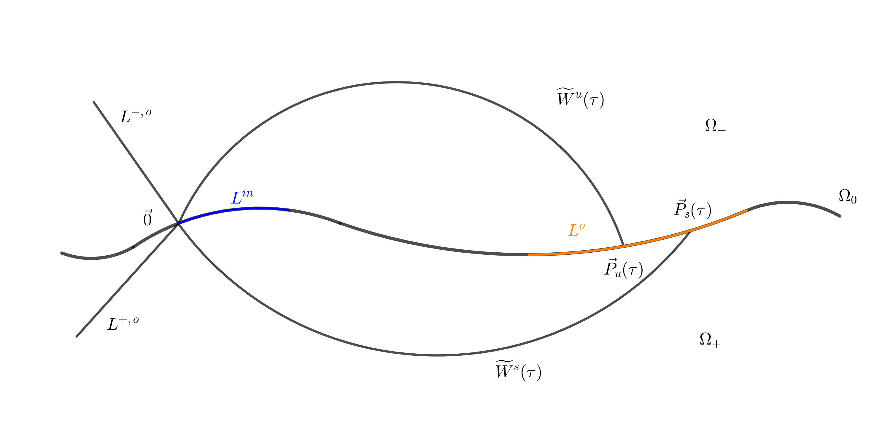
Figure 1: Stable and unstable leaves (the superscript “${}^{\textrm{out}}$” is denoted as “${}^{\textrm{o}}$” for short).

We recall that ${\boldsymbol{\Gamma}}:=\{\vec{\gamma}(t)\mid t\in{\mathbb{R}}\}\cup\{\vec{0}\}$; let us denote by $E^{\textrm{in}}$ the open set enclosed by ${\boldsymbol{\Gamma}}$, and by $E^{\textrm{out}}$ the open set complementary to $E^{\textrm{in}}\cup{\boldsymbol{\Gamma}}$.

Further, for any fixed $\delta>0$, we set

$$\begin{split}L^{0}=L^{0}(\delta)&:=\{\vec{Q}\in\Omega^{0}\mid\|\vec{Q}-\vec{\gamma}(0)\|<\delta\},\\ L^{\textrm{in}}=L^{\textrm{in}}(\delta)&:=\{\vec{Q}\in(\Omega^{0}\cap E^{\textrm{in}})\mid\|\vec{Q}\|<\delta\}.\end{split}$$ (2.2)

We denote by $\vec{x}(t,\tau;\vec{P})$ the trajectory of (PS) which is in $\vec{P}$ at $t=\tau$. Now, we define the stable and the unstable leaves $W^{s}(\tau)$ and $W^{u}(\tau)$ of (PS).

Assume first for simplicity that the system is smooth and suppose that F0 holds true. Then, following [9, §2], which is based on [19, Theorem 2.16], we can define the global stable and unstable leaves as follows:

$$\begin{array}[]{c}W^{u}(\tau):=\{\vec{P}\in{\mathbb{R}}^{2}\mid{\lim_{t\to-\infty}}\vec{x}(t,\tau;\vec{P})=\vec{0}\},\\ W^{s}(\tau):=\{\vec{P}\in{\mathbb{R}}^{2}\mid{\lim_{t\to+\infty}}\vec{x}(t,\tau;\vec{P})=\vec{0}\}.\end{array}$$ (2.3)

In fact $W^{u}(\tau)$ and $W^{s}(\tau)$ are $C^{r}$ immersed $1$-dimensional manifolds, i.e., they are the image of $C^{r}$ curves; they also have $C^{r}$ dependence on $\tau$ and $\varepsilon$ but we leave this last dependence unsaid. Notice that if $\vec{P}\in W^{u}(\tau)$ then $\vec{x}(t,\tau;\vec{P})\in W^{u}(t)$ for any $t,\tau\in{\mathbb{R}}$. Analogously for $W^{s}(\tau)$.

Assume further F1, K and follow $W^{u}(\tau)$ (respectively $W^{s}(\tau)$) from the origin towards $L^{0}(\sqrt{\varepsilon})$: then it intersects $L^{0}(\sqrt{\varepsilon})$ transversely in a point denoted by $\vec{P}_{u}(\tau)$ (respectively by $\vec{P}_{s}(\tau)$). In fact, $\vec{P}_{u}(\tau)$ and $\vec{P}_{s}(\tau)$ are $C^{r}$ functions of $\varepsilon$ and $\tau$; hence $\vec{P}_{u}(\tau)=\vec{P}_{s}(\tau)=\vec{\gamma}(0)$ if $\varepsilon=0$ for any $\tau\in{\mathbb{R}}$.

We denote by $\tilde{W}^{u}(\tau)$ the branch of $W^{u}(\tau)$ between the origin and $\vec{P}_{u}(\tau)$ (a path), and by $\tilde{W}^{s}(\tau)$ the branch of $W^{s}(\tau)$ between the origin and $\vec{P}_{s}(\tau)$, in both the cases including the endpoints. Since $\tilde{W}^{u}(\tau)$ and $\tilde{W}^{s}(\tau)$ coincide with ${\boldsymbol{\Gamma}}\cap(\Omega^{-}\cup\Omega^{0})$ and ${\boldsymbol{\Gamma}}\cap(\Omega^{+}\cup\Omega^{0})$ if $\varepsilon=0$, respectively, and vary in a $C^{r}$ way we find $\tilde{W}^{u}(\tau)\subset(\Omega^{-}\cup\Omega^{0})$ and $\tilde{W}^{s}(\tau)\subset(\Omega^{+}\cup\Omega^{0})$, for any $\tau\in{\mathbb{R}}$ and any $0\leq\varepsilon\leq\varepsilon_{0}$, see again [9] or [13, Appendix]. Further

$$\begin{gathered}\vec{Q}_{u}\in\tilde{W}^{u}(\tau)\Rightarrow\vec{x}(t,\tau;\vec{Q}_{u})\in\tilde{W}^{u}(t)\subset(\Omega^{-}\cup\Omega^{0})\quad\textrm{for any $t\leq\tau$},\\ \vec{Q}_{s}\in\tilde{W}^{s}(\tau)\Rightarrow\vec{x}(t,\tau;\vec{Q}_{s})\in\tilde{W}^{s}(t)\subset(\Omega^{+}\cup\Omega^{0})\quad\textrm{for any $t\geq\tau$}.\end{gathered}$$ (2.4)

Now, we go back to the general case where (PS) is piecewise smooth but discontinuous.

Remark 2.2.

Consider (PS) and assume F0, F1, F2. Following [9] we can again define $\tilde{W}^{u}(\tau)$ and $\tilde{W}^{s}(\tau)$, and we get that they are $C^{r}$ and have the property (2.4).

Moreover, if K holds then $\vec{P}_{u}(\tau)$ and $\vec{P}_{s}(\tau)$ are again $C^{r}$ in $\varepsilon$ and $\tau$, and $\vec{P}_{u}(\tau)=\vec{P}_{s}(\tau)=\vec{\gamma}(0)$ if $\varepsilon=0$ for any $\tau\in{\mathbb{R}}$.

We set

$$\tilde{W}(\tau):=\tilde{W}^{u}(\tau)\cup\tilde{W}^{s}(\tau).$$ (2.5)

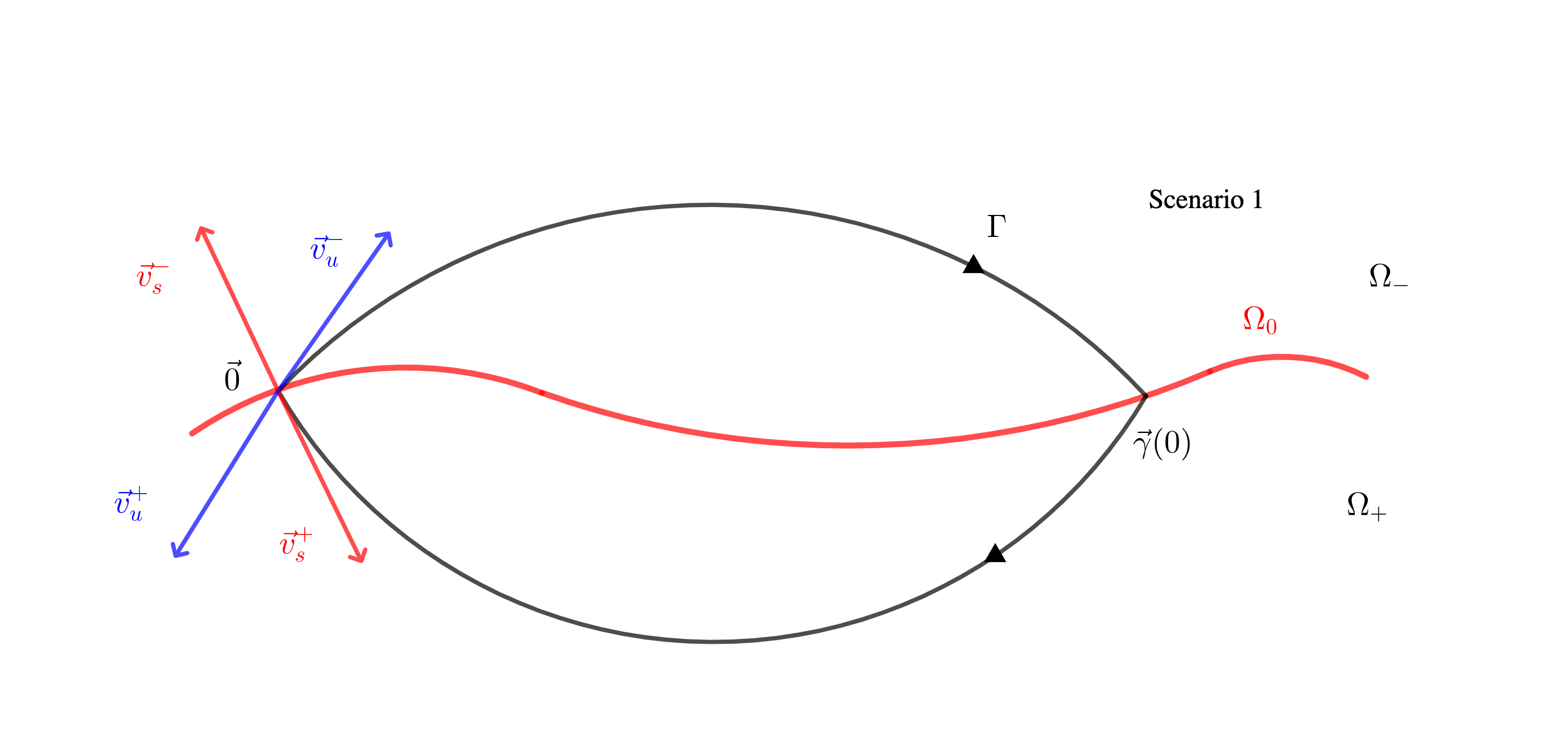
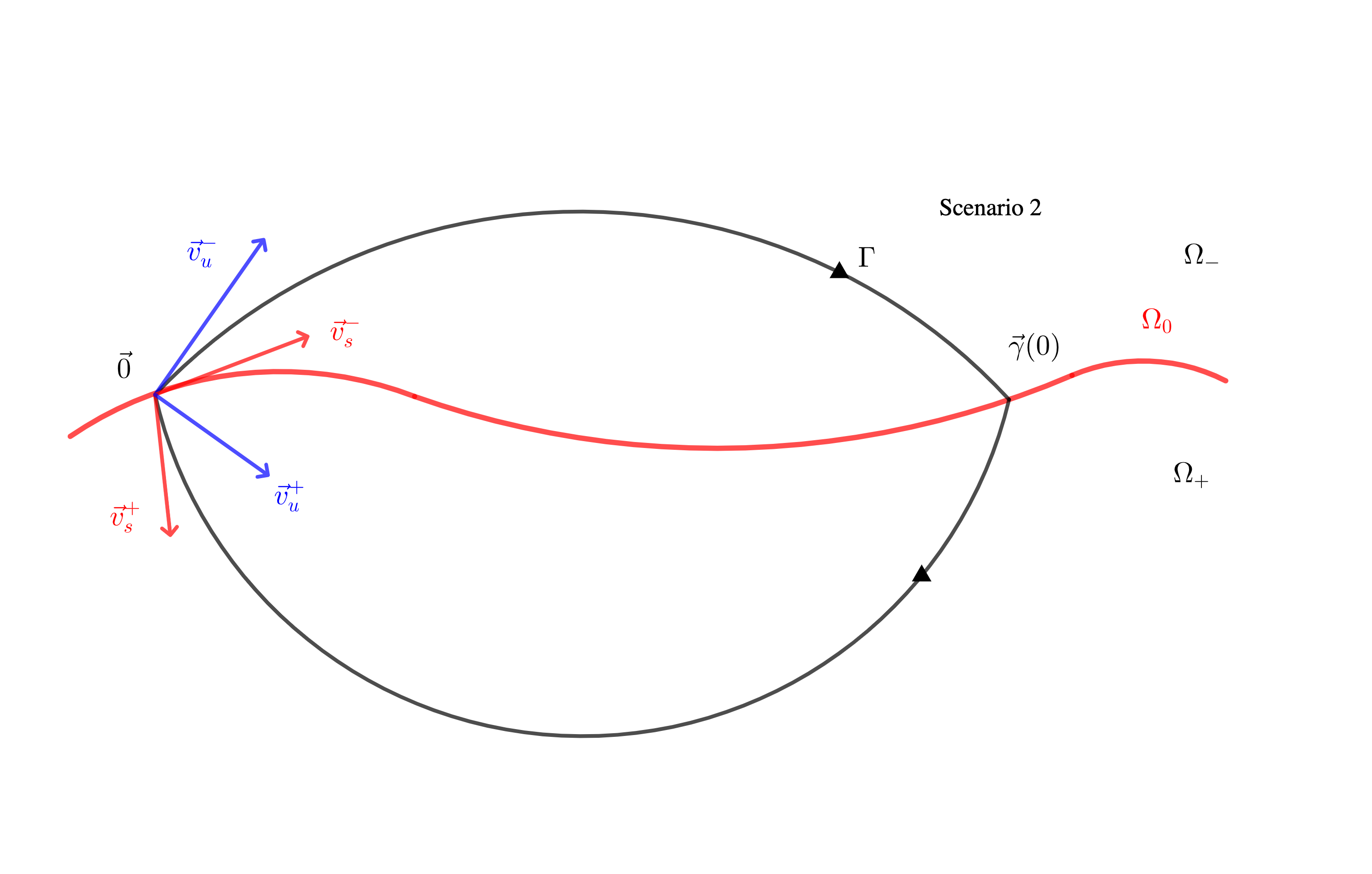
Figure 2: Scenarios 1 and 2. In these two settings there is no sliding close to the origin. Further Melnikov theory guarantees persistence of the homoclinic trajectories [8], and we conjecture that we may have chaotic phenomena.

At this point, we need to distinguish between four possible scenarios, see Figures 2 and 3.

Scenario 1

Assume K and that there is $\rho>0$ such that $d\vec{v}_{u}^{+}\in E^{\textrm{out}}$, $d\vec{v}_{s}^{-}\in E^{\textrm{out}}$ for any $0<d<\rho$.

Scenario 2

Assume K and that there is $\rho>0$ such that $d\vec{v}_{u}^{+}\in E^{\textrm{in}}$, $d\vec{v}_{s}^{-}\in E^{\textrm{in}}$ for any $0<d<\rho$.

Scenario 3

Assume K and that there is $\rho>0$ such that $d\vec{v}_{u}^{+}\in E^{\textrm{in}}$, $d\vec{v}_{s}^{-}\in E^{\textrm{out}}$ for any $0<d<\rho$, so F2 does not hold.

Scenario 4

Assume K and that there is $\rho>0$ such that $d\vec{v}_{u}^{+}\in E^{\textrm{out}}$, $d\vec{v}_{s}^{-}\in E^{\textrm{in}}$ for any $0<d<\rho$, so F2 does not hold.

Notice that F2 holds in both Scenarios 1 and 2, and our results apply to both the cases. Further, let

$$W^{u,+}_{loc}(\tau):=W^{u}(\tau)\cap\Omega^{+}\cap B(\vec{0},\rho),\quad W^{s,-}_{loc}(\tau):=W^{s}(\tau)\cap\Omega^{-}\cap B(\vec{0},\rho)$$

for some $\rho>0$; in Scenario 1 both $W^{u,+}_{loc}(\tau)$ and $W^{s,-}_{loc}(\tau)$ lie in $E^{\textrm{out}}$ for any $\tau\in{\mathbb{R}}$, while in Scenario 2 $W^{u,+}_{loc}(\tau)$ and $W^{s,-}_{loc}(\tau)$ both lie in $E^{\textrm{in}}$ for any $\tau\in{\mathbb{R}}$.

In Scenarios 3 and 4 sliding generically occurs in $\Omega^{0}$ close to the origin, F2 does not hold, and $W^{u,+}_{loc}(\tau)$ and $W^{s,-}_{loc}(\tau)$ lie on the opposite sides with respect to ${\boldsymbol{\Gamma}}$. Notice that Scenarios 1 and 2 have a smooth counterpart while Scenarios 3 and 4 may take place just if the system is discontinuous. We recall once again that in all the four scenarios the existence of a non degenerate zero of the Melnikov function guarantees the persistence of the homoclinic trajectory, cf. [8], but generically chaos is not possible in Scenarios 3 and 4; we conjecture that chaos is still possible in Scenarios 1 and 2: this will be the object of future investigation which will use the results of this article.

In this paper we will just consider Scenario 1 to fix the ideas although Scenario 2 can be handled in a similar way; accordingly we introduce the following notation, see Figure 1.

$$\begin{split}L^{-,\textrm{out}}=L^{-,\textrm{out}}(\delta)&:=\{\vec{Q}=d(\vec{v}_{u}^{-}+\vec{v}_{s}^{-})\mid 0\leq d\leq\delta\},\\ L^{+,\textrm{out}}=L^{+,\textrm{out}}(\delta)&:=\{\vec{Q}=d(\vec{v}_{u}^{+}+\vec{v}_{s}^{+})\mid 0\leq d\leq\delta\}.\end{split}$$

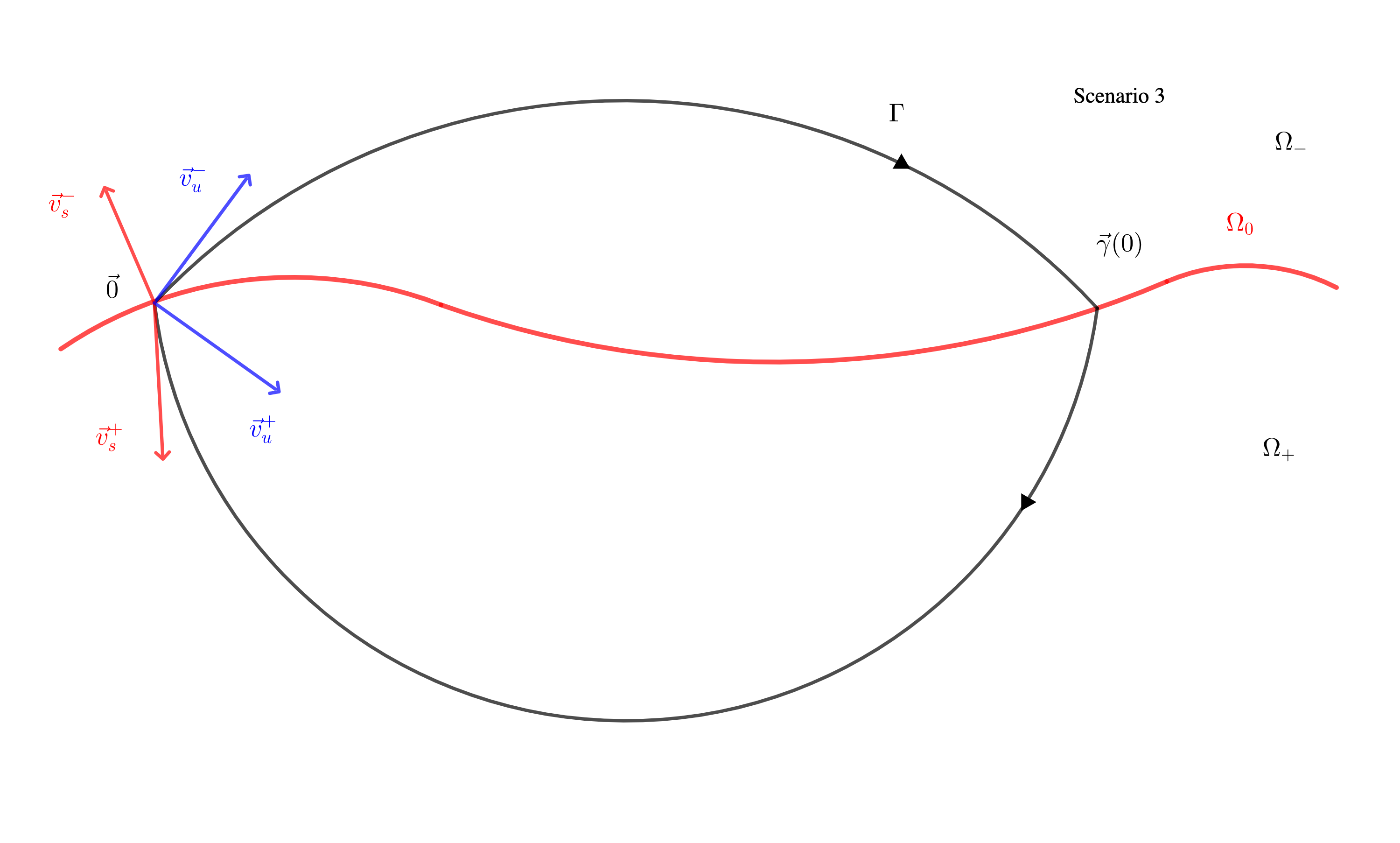
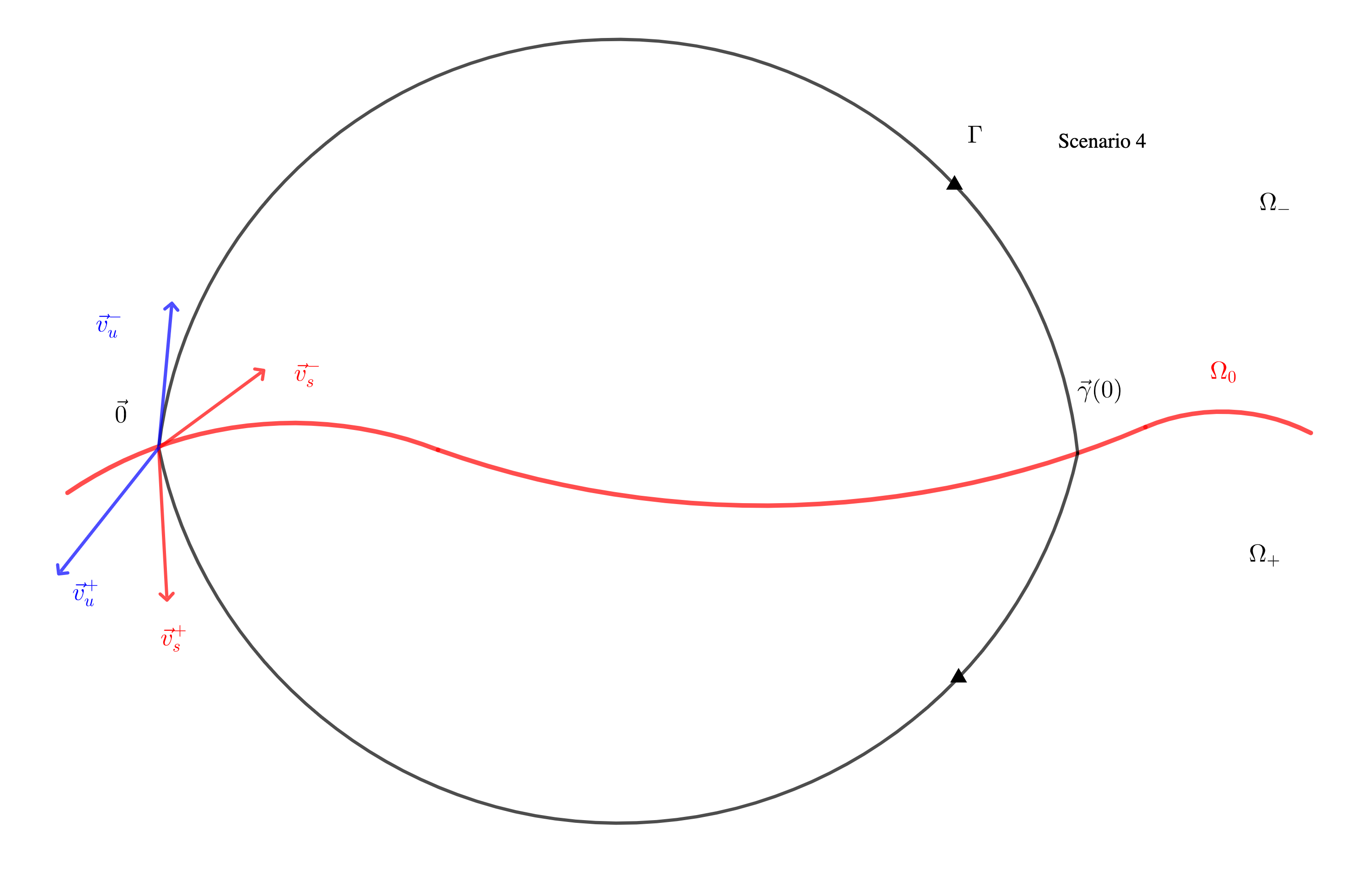
Figure 3: Scenarios 3 and 4. In these settings we have persistence of the homoclinic trajectories but sliding might occur close to the origin. Here our analysis does not apply directly. Further Melnikov theory guarantees persistence of the homoclinic trajectories, cf. [8], but chaos is forbidden in general, cf. [12].

3 Statement of the main results

In this section we state the main results proved in this article. First we collect here for convenience of the reader and future reference, the main constants which will play a role in our argument:

$$\begin{array}[]{ccc}\sigma^{\textrm{fwd}}_{+}=\frac{|\lambda_{s}^{+}|}{\lambda_{u}^{+}+|\lambda_{s}^{+}|},&\sigma^{\textrm{fwd}}_{-}=\frac{\lambda_{u}^{-}+|\lambda_{s}^{-}|}{\lambda_{u}^{-}},&\sigma^{\textrm{fwd}}=\sigma^{\textrm{fwd}}_{+}\sigma^{\textrm{fwd}}_{-},\\ \sigma^{\textrm{bwd}}_{+}=\frac{1}{\sigma^{\textrm{fwd}}_{+}},&\sigma^{\textrm{bwd}}_{-}=\frac{1}{\sigma^{\textrm{fwd}}_{-}},&\sigma^{\textrm{bwd}}=\sigma^{\textrm{bwd}}_{+}\sigma^{\textrm{bwd}}_{-},\\ \underline{\sigma}=\min\{\sigma^{\textrm{fwd}}_{+},\sigma^{\textrm{bwd}}_{-}\},&&\overline{\sigma}=\max\{\sigma^{\textrm{fwd}}_{+},\sigma^{\textrm{bwd}}_{-}\},\end{array}$$ (3.1)

$$\begin{array}[]{ccc}\Sigma^{\textrm{fwd}}_{+}=\frac{1}{\lambda_{u}^{+}+|\lambda_{s}^{+}|},&&\Sigma^{\textrm{bwd}}_{-}=\frac{1}{\lambda_{u}^{-}+|\lambda_{s}^{-}|},\\ \Sigma^{\textrm{fwd}}=\frac{\lambda_{u}^{-}+|\lambda_{s}^{+}|}{\lambda_{u}^{-}(\lambda_{u}^{+}+|\lambda_{s}^{+}|)},&&\Sigma^{\textrm{bwd}}=\frac{\lambda_{u}^{-}+|\lambda_{s}^{+}|}{|\lambda_{s}^{+}|(\lambda_{u}^{-}+|\lambda_{s}^{-}|)},\\ \underline{\Sigma}=\min\{\Sigma^{\textrm{fwd}},\Sigma^{\textrm{bwd}}\},&&\overline{\Sigma}=\max\{\Sigma^{\textrm{fwd}},\Sigma^{\textrm{bwd}}\}.\end{array}$$

Notice that, in particular, $\underline{\sigma}\leq\overline{\sigma}<1$.

Remark 3.1.

In the smooth setting we have $\lambda_{u}^{+}=\lambda_{u}^{-}$, and $\lambda_{s}^{+}=\lambda_{s}^{-}$ so we have the following simplifications

$$\begin{array}[]{c}\sigma^{\textrm{fwd}}=\frac{|\lambda_{s}|}{\lambda_{u}},\quad\sigma^{\textrm{bwd}}=\frac{\lambda_{u}}{|\lambda_{s}|};\qquad\Sigma^{\textrm{fwd}}=\frac{1}{\lambda_{u}},\quad\Sigma^{\textrm{bwd}}=\frac{1}{|\lambda_{s}|}.\end{array}$$ (3.2)

We denote by ${\mathbb{Z}}^{-}=\{k\in{\mathbb{Z}}\mid k\leq-1\}$, ${\mathbb{Z}}^{+}=\{k\in{\mathbb{Z}}\mid k\geq 1\}$, and then by ${\mathcal{E}}^{-}=\{0,1\}^{{\mathbb{Z}}^{-}}$, ${\mathcal{E}}^{+}=\{0,1\}^{{\mathbb{Z}}^{+}}$, respectively, the space of sequences from ${\mathbb{Z}}^{-}$, ${\mathbb{Z}}^{+}$ to $\{0,1\}$.

Let us define the Melnikov function $\mathcal{M}:{\mathbb{R}}\to{\mathbb{R}}$ which, for planar piecewise-smooth systems as (PS), takes the following form, see e.g. [8]:

$$\begin{split}\mathcal{M}(\alpha)&=\int_{-\infty}^{0}{\,\textrm{\rm e}}^{-\int_{0}^{t}\operatorname{tr}\boldsymbol{\vec{f}_{x}^{-}}(\vec{\gamma}^{-}(s))ds}\vec{f}^{-}(\vec{\gamma}(t))\wedge\vec{g}(t+\alpha,\vec{\gamma}^{-}(t),0)dt\\ &\quad{}+\int_{0}^{+\infty}{\,\textrm{\rm e}}^{-\int_{0}^{t}\operatorname{tr}\boldsymbol{\vec{f}_{x}^{+}}(\vec{\gamma}^{+}(s))ds}\vec{f}^{+}(\vec{\gamma}(t))\wedge\vec{g}(t+\alpha,\vec{\gamma}^{+}(t),0)dt,\end{split}$$ (3.3)

where “$\wedge$” is the wedge product in ${\mathbb{R}}^{2}$ defined by $\vec{a}\wedge\vec{b}=a_{1}b_{2}-a_{2}b_{1}$ for any vectors $\vec{a}=(a_{1},a_{2})$, $\vec{b}=(b_{1},b_{2})$. In fact, also in the piecewise-smooth case the function $\mathcal{M}$ is $C^{r}$.

More precisely we will assume that the Melnikov function, defined in (3.3), verifies the following hypothesis.

P1

There is a constant $\bar{c}>0$ and an increasing sequence $(b_{i})$, $i\in{\mathbb{Z}}$, such that $b_{i+1}-b_{i}\geq 1/10$ and

$${\mathcal{M}}(b_{2i})<-\bar{c}<0<\bar{c}<{\mathcal{M}}(b_{2i+1}),$$

for any $i\in{\mathbb{Z}}$.

Remark 3.2.

Notice that $b_{i}\to\pm\infty$ as $i\to\pm\infty$. Further the assumption $b_{i+1}-b_{i}\geq 1/10$ could be replaced by $b_{i+1}-b_{i}\geq c$ where $c>0$ is a constant independent of $i$.

If P1 holds, the intermediate value theorem implies that ${\mathcal{M}}(\tau)$ has at least one zero in $]b_{k},b_{k+1}[$ for any $k\in{\mathbb{Z}}$.

We begin by stating the consequences of our results for (PS), but replacing P1 by more restrictive recurrence properties, for clarity and in order to illustrate the novelties introduced by our approach with more usual periodicity assumptions.

P2

There are $b_{0}$, $b_{1}$ such that ${\mathcal{M}}(b_{0})<0<{\mathcal{M}}(b_{1})$ and $\vec{g}(t,\vec{x},\varepsilon)$ is almost periodic in $t$, i.e. for any $\varsigma>0$ there is $\bar{N}=\bar{N}(\varsigma)>0$ such that

$$\|\vec{g}(t,\vec{x},\varepsilon)-\vec{g}(t+\bar{N},\vec{x},\varepsilon)\|\leq\varsigma\,,\quad\textrm{for any }(t,\vec{x},\varepsilon)\in{\mathbb{R}}\times\Omega\times{\mathbb{R}}.$$

P3

There are $b_{0}$, $b_{1}$ such that ${\mathcal{M}}(b_{0})<0<{\mathcal{M}}(b_{1})$ and $\vec{g}(t,\vec{x},\varepsilon)$ is $1$-periodic in $t$, i.e

$$\vec{g}(t,\vec{x},\varepsilon)=\vec{g}(t+1,\vec{x},\varepsilon)\,,\quad\textrm{for any }(t,\vec{x},\varepsilon)\in{\mathbb{R}}\times\Omega\times{\mathbb{R}}.$$

It is classically known that the periodicity and the almost periodicity of $\vec{g}$ imply the periodicity and the almost periodicity of ${\mathcal{M}}$, so P3 implies P2, which implies P1.

We want to consider an increasing sequence of times $\mathcal{T}=(T_{j})$, $j\in{\mathbb{Z}}$ such that ${\mathcal{M}}(T_{2j})=0$ and $T_{j+1}-T_{j}$ becomes larger and larger as $\varepsilon\to 0$, see (3.11) and (3.12) below. Correspondingly, we find a subsequence $\beta_{j}:=b_{n_{j}}$ such that

$$\beta_{j}:=b_{n_{j}}<T_{j}<\beta^{\prime}_{j}:=b_{n_{j}+1}\,,\qquad B_{j}=\beta^{\prime}_{j}-\beta_{j}=b_{n_{j}+1}-b_{n_{j}}>0,$$ (3.4)

for any $j\in{\mathbb{Z}}$.

When dealing with assumption P1 we follow two different settings of assumptions; the first is slightly more restrictive but includes the cases where $(B_{j})$ is bounded, so in particular it is satisfied if we assume either P2 or P3: it allows to obtain more precise (and clearer) results, i.e., Theorems 3.4 and 3.5; in the second approach we ask for weaker assumptions but we obtain weaker results, i.e., Theorem 3.6 (where we have a very weak control of the size of $\alpha^{{\mathrm{e}}}_{j}(\varepsilon)$ introduced below).

We consider now the first setting of assumptions.

We assume first that there may be some $j\in{\mathbb{Z}}$ such that $T_{2j}$ is an accumulation point of the zeros of ${\mathcal{M}}(\tau)$, so there are $0<\delta<1$, $1/2>\Lambda^{1}>2\Lambda^{0}\geq 0$ and increasing sequences $(a^{\uparrow}_{j})$, $(a^{\downarrow}_{j})$, $j\in{\mathbb{Z}}$ such that

$$\beta_{2j}<a^{\uparrow}_{j}<T_{2j}-\Lambda^{0}<T_{2j}<T_{2j}+\Lambda^{0}<a^{\downarrow}_{j}<\beta^{\prime}_{2j}$$

and

$$\begin{split}&|{\mathcal{M}}(a^{\uparrow}_{j})|=|{\mathcal{M}}(a^{\downarrow}_{j})|=\delta\bar{c},\qquad{\mathcal{M}}(a^{\uparrow}_{j}){\mathcal{M}}(a^{\downarrow}_{j})<0,\\ &{\mathcal{M}}(\tau)\neq 0\quad\forall\tau\in[a^{\uparrow}_{j},a^{\downarrow}_{j}]\setminus[T_{2j}-\Lambda^{0},T_{2j}+\Lambda^{0}],\\ &\textrm{$0<a^{\downarrow}_{j}-a^{\uparrow}_{j}\leq\Lambda^{1}$, for any $j\in{\mathbb{Z}}$.}\end{split}$$ (3.5)

We emphasize that both $\Lambda^{1}$ and $\Lambda^{0}$ are independent of $j\in{\mathbb{Z}}$.

In fact (3.5) is enough to construct a chaotic pattern, but we obtain sharper results if we assume that there is a strictly monotone increasing and continuous function $\omega_{M}(h):[0,\Lambda^{1}]\to[0,+\infty[$ (independent of $j$) such that $\omega_{M}(0)=0$ and

$$\begin{split}|{\mathcal{M}}(T_{2j}-\Lambda^{0}-h)|&\geq\omega_{M}(h)\quad\textrm{for any }\;(T_{2j}-\Lambda^{0}-h)\in[a^{\uparrow}_{j},T_{2j}-\Lambda^{0}],\\ |{\mathcal{M}}(T_{2j}+\Lambda^{0}+h)|&\geq\omega_{M}(h)\quad\textrm{for any }\;(T_{2j}+\Lambda^{0}+h)\in[T_{2j}+\Lambda^{0},a^{\downarrow}_{j}],\end{split}$$ (3.6)

and any $j\in{\mathbb{Z}}$.

Notice that (3.5) and (3.6) are always satisfied if P2 or P3 holds. In fact (3.5) and (3.6) can be satisfied even if the sequence $(B_{j})$ becomes unbounded, but they require a control from below on the “slope” of the Melnikov function “close to its zeros”.

We stress that in the easier and most significant case where $T_{2j}$ is an isolated zero for ${\mathcal{M}}(\cdot)$ for any $j$ we can assume $\Lambda^{0}=0$ so that (3.5) simplifies as follows

$$\begin{split}&|{\mathcal{M}}(a^{\uparrow}_{j})|=|{\mathcal{M}}(a^{\downarrow}_{j})|=\delta\bar{c},\qquad{\mathcal{M}}(a^{\uparrow}_{j}){\mathcal{M}}(a^{\downarrow}_{j})<0,\\ &{\mathcal{M}}(\tau)\neq 0\qquad\forall\tau\in[a^{\uparrow}_{j},a^{\downarrow}_{j}]\setminus\{T_{2j}\}.\end{split}$$ (3.7)

Further in this case (3.6) reduces to

$$|{\mathcal{M}}(T_{2j}+h)|\geq\omega_{M}(|h|)\quad\textrm{for any }(T_{2j}+h)\in[a^{\uparrow}_{j},a^{\downarrow}_{j}]\,,\quad h\neq 0,$$ (3.8)

and any $j\in{\mathbb{Z}}$.

When we assume the classical hypothesis that there is $C>0$ such that

$${\mathcal{M}}(T_{2j})=0\quad\text{and}\quad|{\mathcal{M}}^{\prime}(T_{2j})|>C\;\text{for any $j\in{\mathbb{Z}}$,}$$ (3.9)

then (3.5) and (3.8) hold and we may assume simply $\omega_{M}(h)=\tfrac{C}{2}h$ and $\Lambda^{1}=2\frac{\bar{c}}{C}\delta<\tfrac{1}{2}$.

Now we need to define the following absolute constants $K_{0}$ and $\nu_{0}$, which depend only on the eigenvalues in F0:

$$K_{0}:=\frac{3\overline{\Sigma}}{2\underline{\sigma}},\qquad\nu_{0}:=\max\left\{3\overline{\sigma}-1;1\right\}.$$ (3.10)

Following [9] we introduce a further parameter $\nu\geq\nu_{0}$ which is used to tune the distance of the points in $\vec{\xi}\in\Sigma^{+}$ from $\vec{P}_{s}(\tau)$, paying the price of a longer time needed by the trajectory $\vec{x}(t,\tau;\vec{\xi})$ to perform a loop in forward time (and analogously for $\vec{\xi}\in\Sigma^{-}$ in backward time).

When P1 and (3.5) hold we need the following condition concerning the sequence $(T_{j})$ and the time gap $T_{j+1}-T_{j}$:

$${\mathcal{M}}(T_{2j})=0,\qquad T_{j+1}-T_{j}>\Lambda^{1}+K_{0}(1+\nu)|\ln(\varepsilon)|,\quad\textrm{ for any $j\in{\mathbb{Z}}$},\quad\nu\geq\nu_{0}.$$ (3.11)

Remark 3.3.

If P3 holds and there is $t_{0}$ such that ${\mathcal{M}}(t_{0})=0\neq{\mathcal{M}}^{\prime}(t_{0})$, then we can choose ${\mathcal{T}}=(T_{j})$, $T_{j}=t_{0}+j\Theta$, where $\Theta=\left[K_{0}(1+\nu)|\ln(\varepsilon)|+2\right]$, where $[\cdot]$ denotes the integer part, so that it satisfies (3.11) and (3.9).

In the second approach we drop (3.5), but we need to ask for a slightly more restrictive condition on the time gap $T_{j+1}-T_{j}$, i.e.:

$$\begin{split}&{\mathcal{M}}(T_{2j})=0,\qquad T_{j+1}-T_{j}>\max\{B_{j+1};B_{j}\}+K_{0}(1+\nu)|\ln(\varepsilon)|,\end{split}$$ (3.12)

for any $j\in\mathbb{Z}$ and $\nu\geq\nu_{0}$.

Let us denote by $\tilde{V}(\tau)$ the compact connected set enclosed by $\tilde{W}(\tau)$ and by the branch of $\Omega^{0}$ between $\vec{P}_{u}(\tau)$ and $\vec{P}_{s}(\tau)$. Now we are ready to state the main results of the paper, i.e., Theorems 3.4, 3.5, 3.6 and Corollaries 3.7, 3.12, 3.13; the proofs of all these results are postponed to Section 5. More precisely Theorem 3.4 is proved in §5.2, Theorem 3.6 a) is proved at the end of §5.1, while Theorem 3.6 b) together with all the other results are proved in §5.3.

Theorem 3.4.

Assume that $\vec{f}^{\pm}$ and $\vec{g}$ are $C^{r}$, $r>1$ and that F0, F1, F2, K and G hold true; assume further P1, and fix $\nu\geq\nu_{0}$ for $\nu_{0}$ as in (3.10) and $\tau\in[b_{0},b_{1}]$. Then we can choose $\varepsilon_{0}$ small enough so that for any $0<\varepsilon\leq\varepsilon_{0}$ and any increasing sequence $\mathcal{T}^{+}=(T_{j})$ satisfying (3.11) for $j\in{\mathbb{Z}}^{+}$ and

$$T_{1}-b_{1}>\Lambda^{1}+K_{0}(1+\nu)|\ln(\varepsilon)|,\quad\text{ for any }\nu\geq\nu_{0},$$ (3.13)

there is $c^{*}>0$ so that the following holds. For any sequence ${\mathrm{e}}^{+}\in{\mathcal{E}}^{+}$ there is a compact set $X^{+}=X^{+}({\mathrm{e}}^{+},\tau,{\mathcal{T}}^{+})$ and a sequence $\alpha_{j}(\varepsilon)=\alpha_{j}^{{\mathrm{e}}^{+}}(\varepsilon,\tau,{\mathcal{T}}^{+})$ such that for any $\vec{\xi}\in X^{+}$ the trajectory $\vec{x}(t,\tau;\vec{\xi})\in\tilde{V}(t)$ for any $t\geq\tau$ and satisfies the property ${\boldsymbol{C_{{\mathrm{e}}^{+}}^{+}}}$, i.e.

${\boldsymbol{C_{{\mathrm{e}}^{+}}^{+}}}$

if ${\mathrm{e}}_{j}=1$ then

$$\begin{split}&\|\vec{x}(t,\tau;\vec{\xi})-\vec{\gamma}(t-T_{2j}-\alpha_{j}(\varepsilon))\|\leq c^{*}\varepsilon\quad\textrm{when $t\in[T_{2j-1},T_{2j+1}]$},\end{split}$$ (3.14)

while if ${\mathrm{e}}_{j}=0$ we have

$$\|\vec{x}(t,\tau;\vec{\xi})\|\leq c^{*}\varepsilon\quad\textrm{when $t\in[T_{2j-1},T_{2j+1}]$}$$ (3.15)

for any $j\in{\mathbb{Z}}^{+}$. Further

$$\|\vec{x}(t,\tau;\vec{\xi})-\vec{\gamma}(t-\tau)\|\leq c^{*}\varepsilon\quad\textrm{when $t\in[\tau,T_{1}]$}.$$ (3.16)

Moreover for any $j\in\mathbb{Z}^{+}$ we have the following estimates

a)

if (3.9) holds and $r\geq 2$ there is $c_{\alpha}>0$ such that $|\alpha_{j}^{{\mathrm{e}}^{+}}(\varepsilon)|\leq c_{\alpha}\varepsilon$;

b)

if (3.8) holds and $r>1$ then

$$|\alpha_{j}^{{\mathrm{e}}^{+}}(\varepsilon)|\leq\omega_{\alpha}(\varepsilon),$$

where $\omega_{\alpha}(\cdot)$ is an increasing continuous function such that $\omega_{\alpha}(0)=0$;

c)

if (3.5) holds and $r>1$ then $|\alpha_{j}^{{\mathrm{e}}^{+}}(\varepsilon)|\leq\Lambda^{1}$.

The constants $\varepsilon_{0}$, $c^{*}$, $c_{\alpha}$ and the function $\omega_{\alpha}$ are independent of $\varepsilon$, $\nu$, $\tau$, ${\mathcal{T}}^{+}$, ${\mathrm{e}}^{+}$.

Theorem 3.5.

Assume that $\vec{f}^{\pm}$ and $\vec{g}$ are $C^{r}$, $r>1$ and that F0, F1, F2, K and G hold true; assume further P1 and fix $\nu\geq\nu_{0}$ for $\nu_{0}$ as in (3.10) and $\tau\in[b_{0},b_{1}]$. Then we can choose $\varepsilon_{0}$ small enough so that for any $0<\varepsilon\leq\varepsilon_{0}$ and any increasing sequence $\mathcal{T}^{-}=(T_{j})$ satisfying (3.11) for $j\leq-2$ and

$$b_{0}-T_{-1}>\Lambda^{1}+K_{0}(1+\nu)|\ln(\varepsilon)|,\quad\text{ for any }\nu\geq\nu_{0},$$ (3.17)

there is $c^{*}>0$ so that the following holds. For any sequence ${\mathrm{e}}^{-}\in{\mathcal{E}}^{-}$ there is a compact set $X^{-}=X^{-}({\mathrm{e}}^{-},\tau,{\mathcal{T}}^{-})$ and a sequence $\alpha_{j}(\varepsilon)=\alpha_{j}^{{\mathrm{e}}^{-}}(\varepsilon,\tau,{\mathcal{T}}^{-})$ such that for any $\vec{\xi}\in X^{-}$ the trajectory $\vec{x}(t,\tau;\vec{\xi})\in\tilde{V}(t)$ for any $t\leq\tau$ and satisfies the property ${\boldsymbol{C_{{\mathrm{e}}^{-}}^{-}}}$, i.e.

${\boldsymbol{C_{{\mathrm{e}}^{-}}^{-}}}$

if ${\mathrm{e}}_{j}=1$, then

$$\begin{split}&\|\vec{x}(t,\tau;\vec{\xi})-\vec{\gamma}(t-T_{2j}-\alpha_{j}(\varepsilon))\|\leq c^{*}\varepsilon\quad\textrm{when $t\in[T_{2j-1},T_{2j+1}]$},\end{split}$$ (3.18)

while if ${\mathrm{e}}_{j}=0$, we have

$$\|\vec{x}(t,\tau;\vec{\xi})\|\leq c^{*}\varepsilon\quad\textrm{when $t\in[T_{2j-1},T_{2j+1}]$}$$ (3.19)

for any $j\in{\mathbb{Z}}^{-}$. Further

$$\|\vec{x}(t,\tau;\vec{\xi})-\vec{\gamma}(t-\tau)\|\leq c^{*}\varepsilon\quad\textrm{when $t\in[T_{-1},\tau]$}.$$ (3.20)

Moreover for any $j\in\mathbb{Z}^{-}$ we have the following estimates

a)

if (3.9) holds and $r\geq 2$, there is $c_{\alpha}>0$ such that $|\alpha_{j}^{{\mathrm{e}}^{-}}(\varepsilon)|\leq c_{\alpha}\varepsilon$;

b)

if (3.8) holds and $r>1$, then

$$|\alpha_{j}^{{\mathrm{e}}^{-}}(\varepsilon)|\leq\omega_{\alpha}(\varepsilon),$$

where $\omega_{\alpha}(\cdot)$ is an increasing continuous function such that $\omega_{\alpha}(0)=0$;

c)

if (3.5) holds and $r>1$ then $|\alpha_{j}^{{\mathrm{e}}^{-}}(\varepsilon)|\leq\Lambda^{1}$.

The constants $\varepsilon_{0}$, $c^{*}$, $c_{\alpha}$ and the function $\omega_{\alpha}$ are independent of $\varepsilon$, $\nu$, $\tau$, ${\mathcal{T}}^{-}$, ${\mathrm{e}}^{-}$.

Theorem 3.6.

a)

Assume that the hypotheses of Theorem 3.4 hold but replace (3.11) by (3.12) and (3.13) by

$$T_{1}-b_{1}>\max\{B_{1};B_{0}\}+K_{0}(1+\nu)|\ln(\varepsilon)|,\quad\text{ for any }\nu\geq\nu_{0},$$ (3.21)

then we obtain the same result as in Theorem 3.4 but we just have

$$|\alpha_{j}^{{\mathrm{e}}^{+}}(\varepsilon)|\leq B_{2j}.$$

b)

Assume that the hypotheses of Theorem 3.5 hold but replace (3.11) by (3.12) and (3.17) by

$$b_{0}-T_{-1}>\max\{B_{0};B_{-1}\}+K_{0}(1+\nu)|\ln(\varepsilon)|,\quad\text{ for any }\nu\geq\nu_{0},$$ (3.22)

then we obtain the same result as in Theorem 3.5 but we just have

$$|\alpha_{j}^{{\mathrm{e}}^{-}}(\varepsilon)|\leq B_{2j}.$$

In Theorems 3.4 and 3.5 we can suppress the dependence on $\alpha_{j}^{{\mathrm{e}}^{\pm}}(\varepsilon)$ of the relations in (3.14), (3.18), possibly paying the price of a further loss of precision of the estimates.

Corollary 3.7.

Let the assumptions of Theorems 3.4 and 3.5 hold.

If a) holds then we can replace (3.14), (3.18), by

$$\begin{split}&\|\vec{x}(t,\tau;\vec{\xi})-\vec{\gamma}(t-T_{2j})\|\leq\tilde{c}^{*}\varepsilon\quad\textrm{when $t\in[T_{2j-1},T_{2j+1}]$}\end{split}$$

where $\tilde{c}^{*}$ is the constant in (5.52).

If b) holds then we can replace (3.14), (3.18), by

$$\begin{split}&\|\vec{x}(t,\tau;\vec{\xi})-\vec{\gamma}(t-T_{2j})\|\leq\omega(\varepsilon)\quad\textrm{when $t\in[T_{2j-1},T_{2j+1}]$}\end{split}$$

where $\omega(\varepsilon)=c^{*}\varepsilon+\tilde{c}\omega_{\alpha}(\varepsilon)$ and $\tilde{c}>0$ is a constant, cf. (5.49).

Remark 3.8.

Notice that if we have two different sequences $\hat{{\mathrm{e}}}^{\pm}$ and $\check{{\mathrm{e}}}^{\pm}$ in ${\mathcal{E}}^{\pm}$ then $X^{\pm}(\hat{{\mathrm{e}}}^{\pm},\tau,{\mathcal{T}}^{\pm})\cap X^{\pm}(\check{{\mathrm{e}}}^{\pm},\tau,{\mathcal{T}}^{\pm})=\emptyset$. We conjecture that in the setting of Theorem 3.4 a) and Theorem 3.5 a) $X^{+}({\mathrm{e}}^{+},\tau,{\mathcal{T}}^{+})$ and $X^{-}({\mathrm{e}}^{-},\tau,{\mathcal{T}}^{-})$ are singletons for any ${\mathrm{e}}^{+}\in{\mathcal{E}}^{+}$ and any ${\mathrm{e}}^{-}\in{\mathcal{E}}^{-}$.

Remark 3.9.

We stress that P1 does not require an upper bound on $B_{j}$ when $|j|\to+\infty$. Further, the self-similarity required on ${\mathcal{M}}$ is very weak and we do not need any non-degeneracy of the zeros of the Melnikov function ${\mathcal{M}}(\tau)$, which may be null in some interval. Hence with our results we can deal with functions like, e.g.:

$$\begin{split}&{\mathcal{M}}_{1}(\tau)=3\sin(\tau)+k(\tau),\\ &{\mathcal{M}}_{2}(\tau)=3\sin(\sqrt[3]{1+\tau^{2}})+k(\tau)\end{split}$$ (3.23)

where $|k(\tau)|\leq 2$ is arbitrary.
Notice that ${\mathcal{M}}_{1}(\tau)$ satisfies (3.5) and (3.6), while ${\mathcal{M}}_{2}(\tau)$ does not even satisfy (3.5). So in the former case we can apply Theorems 3.4 and 3.5 while in the latter just Theorem 3.6.

Further notice that if we assume $k(\tau)\equiv 0$, in the former case we can apply Corollary 3.7 since the hypotheses of Theorems 3.4 a) and 3.5 a) are satisfied, while in the latter we can apply again just Theorem 3.6, since we do not have a uniform lower bound on $|{\mathcal{M}}^{\prime}(T_{j})|$.

Via Theorem 3.4 or 3.6 a) we define the sets

$$\begin{split}\Sigma^{+}(\tau,{\mathcal{T}}^{+}):=&\cup_{{\mathrm{e}}^{+}\in{\mathcal{E}}^{+}}X^{+}({\mathrm{e}}^{+},\tau,{\mathcal{T}}^{+}).\end{split}$$ (3.24)

Analogously via Theorems 3.5 or 3.6 b) we define the sets

$$\Sigma^{-}(\tau,{\mathcal{T}}^{-}):=\cup_{{\mathrm{e}}^{-}\in{\mathcal{E}}^{-}}X^{-}({\mathrm{e}}^{-},\tau,{\mathcal{T}}^{-}).$$ (3.25)

Remark 3.10.

Assume that we are in the setting either of Theorem 3.4 or of Theorem 3.6 a) but assume that the system is smooth. Then we can replace $\Omega^{0}$ by any line (or curve) $\Xi$ transversal to ${\boldsymbol{\Gamma}}\setminus\{\vec{0}\}$ (cf. point 1 of Introduction), so for any fixed couple $(\tau,{\mathcal{T}}^{+})$ we find uncountably many distinct chaotic sets $\Sigma^{+}(\tau,{\mathcal{T}}^{+})$, one for each transversal $\Xi$. The analogous result holds for $\Sigma^{-}(\tau,{\mathcal{T}}^{-})$ when either the assumptions of Theorem 3.5 or of Theorem 3.6 b) are satisfied

Remark 3.11.

Assume that we are in the setting either of Theorem 3.4 or of Theorem 3.6 a), this time allow the system to be non-smooth. For any $T\in{\mathbb{R}}$ we can define

$$\Sigma^{+}_{T}(\tau,{\mathcal{T}}^{+}):=\{\vec{x}(T,\tau;\xi)\mid\xi\in\Sigma^{+}(\tau,{\mathcal{T}}^{+})\}.$$

Now fix $T\in{\mathbb{R}}$ and a point $\vec{\zeta}\in{\boldsymbol{\Gamma}}$, say $\vec{\zeta}=\vec{\gamma}(s)$, $s\in{\mathbb{R}}$. Then the set $\Sigma^{+}_{T}(T-s,{\mathcal{T}}^{+})$ is $O(\varepsilon)$ close to $\vec{\zeta}$. This way for any fixed $T\in{\mathbb{R}}$ we construct uncountably many distinct sets $\Sigma^{+}_{T}(T-s,{\mathcal{T}}^{+})$ parametrized by $s$, each of them $O(\varepsilon)$ close to a point $\zeta=\vec{\gamma}(s)\in{\boldsymbol{\Gamma}}$. An analogous result holds for $\Sigma^{-}$. In this way we extend the results of Remark 3.10 to the piecewise smooth but discontinuous case.

Corollary 3.12.

Let either the assumptions of Theorems 3.4 and 3.5 or the assumptions of Theorem 3.6 hold. Then the sets $\Sigma^{\pm}(\tau,\mathcal{T}^{\pm})=\cup_{{\mathrm{e}}^{\pm}\in{\mathcal{E}}^{\pm}}X^{\pm}({\mathrm{e}}^{\pm},\tau,\mathcal{T}^{\pm})$ are compact and $\Sigma^{\pm}(\tau,\mathcal{T}^{\pm})\subset L^{0}(c^{*}\varepsilon)$. Further

$$\textrm{diam}(\Sigma^{\pm}):=\sup\left\{\|\vec{Q}_{2}-\vec{Q}_{1}\|\mid\vec{Q}_{1},\vec{Q}_{2}\in\Sigma^{\pm}(\tau,{\mathcal{T}}^{\pm})\right\}\leq\varepsilon^{\frac{1+\nu}{\underline{\sigma}}}.$$ (3.26)

Moreover $\vec{P}_{s}(\tau)$ is an extremal point in $\Sigma^{+}(\tau,{\mathcal{T}}^{+})$, while $\vec{P}_{u}(\tau)$ is an extremal point in $\Sigma^{-}(\tau,{\mathcal{T}}^{-})$, and both $\vec{P}_{s}(\tau)$ and $\vec{P}_{u}(\tau)$ correspond to the null sequence.

From Corollary 3.12 we see that the sets $\Sigma^{\pm}(\tau,{\mathcal{T}}^{\pm})$ are located in a one-dimensional set. Further they are contained in a set whose diameter becomes arbitrarily small as $\nu$ increases, leaving unaltered the size $\varepsilon$ of the perturbation. The drawback is that the minimum gap $T_{j+1}-T_{j}$ increases linearly with $\nu$. However the positions of $\vec{P}_{s}(\tau)$ and $\vec{P}_{u}(\tau)$ are known just with a precision of order $O(\varepsilon)$ since they both oscillate in $L^{0}(c^{*}\varepsilon)$.

Further, in the setting of Theorems 3.4 and 3.5 the flow of (PS) on $\Sigma^{+}$ and on $\Sigma^{-}$ is semi-conjugated to the Bernoulli shift on ${\mathcal{E}}^{+}$ and on ${\mathcal{E}}^{-}$ respectively, see Theorem 6.5.

In fact we get an even better localization of the initial conditions giving rise to chaos if we evaluate them at $t=T_{1}$.

Corollary 3.13.

Let either the assumptions of Theorem 3.4 or the assumptions of Theorem 3.6 a) be satisfied; then

$$\Sigma^{+}_{1}:=\{\vec{x}(T_{1},\tau;\vec{\xi})\mid\vec{\xi}\in\Sigma^{+}(\tau,{\mathcal{T}}^{+})\}\subset\left(B(\vec{0},\varepsilon^{\frac{\nu+1}{2}})\cap\tilde{V}(T_{1})\right).$$

Analogously let either the assumptions of Theorem 3.5 or the assumptions of Theorem 3.6 b) be satisfied; then

$$\Sigma^{-}_{-1}:=\{\vec{x}(T_{-1},\tau;\vec{\xi})\mid\vec{\xi}\in\Sigma^{-}(\tau,{\mathcal{T}}^{-})\}\subset\left(B(\vec{0},\varepsilon^{\frac{\nu+1}{2}})\cap\tilde{V}(T_{-1})\right).$$

The proof of this result is postponed to the end of Section 5.

As far as we are aware these facts are new even when $\vec{f}$ is smooth and stress the sensitive dependence of this perturbed equation on initial conditions.

We close this section by observing that, in the smooth context, assumption G is not restrictive. In fact we may replace it by

G’

there is $C_{g}>0$ such that $\|\vec{g}(t,\vec{0},\varepsilon)\|\leq C_{g}$ for any $t\in{\mathbb{R}}$ and any $0\leq\varepsilon\leq 1$.

Note that, in the smooth case and under condition G’, by standard arguments relying on the exponential dichotomy theory, see e.g. [7, §4.2], it can be proved that (S) admits a unique solution, say $\vec{x}_{b}(t,\varepsilon)$, which is bounded for any $t\in{\mathbb{R}}$ and such that $\|\vec{x}_{b}(t,\varepsilon)\|=O(\varepsilon)$ uniformly in $t\in{\mathbb{R}}$. In fact $\vec{x}_{b}(t,\varepsilon)$ emanates from the origin and, roughly speaking, replaces its role; i.e., $\vec{\gamma}(t)$ is perturbed on a trajectory homoclinic to $\vec{x}_{b}(t,\varepsilon)$ as $|t|\to\infty$. Further we have the following.

Remark 3.14.

In the smooth case, replace G by G’; then we can still apply our methods to (S), obtaining a result analogous to Corollary 3.13.

Proof of Remark 3.14.

If G’ holds we may set $\vec{y}(t,\varepsilon)=\vec{x}-\vec{x}_{b}(t,\varepsilon)$ so that (S) is changed into

$$\dot{\vec{y}}=\vec{f}(\vec{y})+\varepsilon\vec{g}_{T}(t,\vec{y},\varepsilon)$$ (3.27)

where

$$\begin{split}\vec{g}_{T}(t,\vec{y},\varepsilon):=&\vec{g}(t,\vec{y}+\vec{x}_{b}(t,\varepsilon),\varepsilon)-\vec{g}(t,\vec{x}_{b}(t,\varepsilon),\varepsilon)\\ &+\frac{\vec{f}(\vec{y}+\vec{x}_{b}(t,\varepsilon))-\vec{f}(\vec{y})-\vec{f}(\vec{x}_{b}(t,\varepsilon))}{\varepsilon}.\end{split}$$

Using the fact that $\vec{x}_{b}(t,\varepsilon)/\varepsilon$ is uniformly bounded, one can check that $\vec{g}_{T}(t,\vec{y},\varepsilon)$ is bounded when $t\in{\mathbb{R}}$, $\vec{y}$ is in a compact neighborhood of ${\boldsymbol{\Gamma}}$ and $\varepsilon\in[0,1]$. Further $\vec{g}_{T}(t,\vec{0},\varepsilon)\equiv 0$ so (3.27) satisfies G. So we can apply the results of this section; then going back to the original coordinates we prove the remark.   Classically with the change of variable used in Remark 3.14 we have a loss of regularity with respect to the $\varepsilon$ variable, which is important to obtain $C^{r-1}$ functions $\alpha_{j}(\varepsilon)$. However our approach does not allow a good control on the functions $\alpha_{j}(\varepsilon)$ which are at most continuous and in fact usually they are not uniquely defined, see Theorems 3.4, 3.5 and 3.6; so we have no problems with the loss of regularity and we can ask for $r>1$ instead of $r\geq 2$.

4 Construction of the Poincaré map

In this section we borrow the results of [9] and we construct a Poincaré map from a subset of $L^{0}$ back to $L^{0}$ both forward and backward in time.

Fix $\tau\in{\mathbb{R}}$ and consider $L^{0}(\delta)$ given by (2.2), where $\delta>0$ is a small parameter, independent of $\varepsilon>0$.

The point $\vec{P}_{s}(\tau)$ ($\vec{P}_{u}(\tau)$) splits $L^{0}$ in two parts, say $A^{\textrm{fwd},+}(\tau)$ and $B^{\textrm{fwd},+}(\tau)$ ($A^{\textrm{fwd},-}(\tau)$ and $B^{\textrm{fwd},-}(\tau)$), respectively “inside” and “outside”. Following [9] we define a $C^{r}$ Poincaré map using the flow of (PS) from $A^{\textrm{fwd},+}(\tau)$ back to $L^{0}$ remaining close to ${\boldsymbol{\Gamma}}$; i.e. $\mathscr{P}^{\textrm{fwd}}(\cdot,\tau):A^{\textrm{fwd},+}(\tau)\to L^{0}$ and a $C^{r}$ time map $\mathscr{T}^{\textrm{fwd}}(\cdot,\tau):A^{\textrm{fwd},+}(\tau)\to{\mathbb{R}}$ such that for any $\vec{P}\in A^{\textrm{fwd},+}(\tau)$ the trajectory $\vec{x}(t,\tau;\vec{P})$ will stay close to ${\boldsymbol{\Gamma}}$ (in fact close to $\tilde{W}(t)$) for any $t\in[\tau,\mathscr{T}^{\textrm{fwd}}(\vec{P},\tau)]$ and it will cross transversely $L^{0}$ for the first time at $t=\mathscr{T}^{\textrm{fwd}}(\vec{P},\tau)>\tau$ in the point $\mathscr{P}^{\textrm{fwd}}(\vec{P},\tau)\in A^{\textrm{fwd},-}(\mathscr{T}^{\textrm{fwd}}(\vec{P},\tau))$.
Notice that if $\vec{P}\in B^{\textrm{fwd},+}(\tau)$ then there is some $\mathscr{T}^{\textrm{out}}=\mathscr{T}^{\textrm{out}}(\vec{P},\tau)>\tau$ such that the trajectory will leave a neighborhood of ${\boldsymbol{\Gamma}}$ at $t\geq\mathscr{T}^{\textrm{out}}$.

Similarly, the point $\vec{P}_{u}(\tau)$ ($\vec{P}_{s}(\tau)$) splits $L^{0}$ in two parts, say $A^{\textrm{bwd},-}(\tau)$ and $B^{\textrm{bwd},-}(\tau)$ ($A^{\textrm{bwd},+}(\tau)$ and $B^{\textrm{bwd},+}(\tau)$), respectively “inside” and “outside”. Using the flow of (PS) (but now going backward in time) we construct a $C^{r}$ Poincaré map $\mathscr{P}^{\textrm{bwd}}(\cdot,\tau):A^{\textrm{bwd},-}(\tau)\to L^{0}$ and a $C^{r}$ time map $\mathscr{T}^{\textrm{bwd}}(\cdot,\tau):A^{\textrm{bwd},-}(\tau)\to{\mathbb{R}}$ such that for any $\vec{P}\in A^{\textrm{bwd},-}(\tau)$ the trajectory $\vec{x}(t,\tau;\vec{P})$ will stay close to ${\boldsymbol{\Gamma}}$ (in fact close to $\tilde{W}(t)$) for any $t\in[\mathscr{T}^{\textrm{bwd}}(\vec{P},\tau),\tau]$ and it will cross transversely $L^{0}$ for the first time at $t=\mathscr{T}^{\textrm{bwd}}(\vec{P},\tau)<\tau$ in the point $\mathscr{P}^{\textrm{bwd}}(\vec{P},\tau)\in A^{\textrm{bwd},+}(\mathscr{T}^{\textrm{bwd}}(\vec{P},\tau))$.
Again if $\vec{P}\in B^{\textrm{bwd},-}(\tau)$ then there is some $\mathscr{T}^{\textrm{out}}(\vec{P},\tau)<\tau$ such that the trajectory will leave a neighborhood of ${\boldsymbol{\Gamma}}$ at $t\leq\mathscr{T}^{\textrm{out}}$.

Lemma 4.1.

[9, Lemma 3.6] Assume F0, F1, F2, K, G. Let $\vec{Q}\in A^{\textrm{fwd},+}(\tau)$. Then there are $\mathscr{T}^{\textrm{fwd}}(\vec{Q},\tau)>\tau_{1}(\vec{Q},\tau)>\tau$ such that the trajectory $\vec{x}(t,\tau;\vec{Q})$ crosses transversely $\Omega^{0}$ at $t\in\{\tau,\tau_{1}(\vec{Q},\tau),\mathscr{T}^{\textrm{fwd}}(\vec{Q},\tau)\}$. Hence,

$$\mathscr{P}^{\textrm{fwd}}_{+}(\vec{Q},\tau):=\vec{x}(\tau_{1}(\vec{Q},\tau),\tau;\vec{Q})\in L^{\textrm{in}},$$

$$\mathscr{P}^{\textrm{fwd}}(\vec{Q},\tau):=\vec{x}(\mathscr{T}^{\textrm{fwd}}(\vec{Q},\tau),\tau;\vec{Q})\in A^{\textrm{fwd},-}(\mathscr{T}^{\textrm{fwd}}(\vec{Q},\tau)).$$

Analogously, let $\vec{Q}\in A^{\textrm{bwd},-}(\tau)$. Then there are $\mathscr{T}^{\textrm{bwd}}(\vec{Q},\tau)<\tau_{-1}(\vec{Q},\tau)<\tau$ such that $\vec{x}(t,\tau;\vec{Q})$, crosses transversely $\Omega^{0}$ at $t\in\{\tau,\tau_{-1}(\vec{Q},\tau),\mathscr{T}^{\textrm{bwd}}(\vec{Q},\tau)\}$. Hence

$$\mathscr{P}^{\textrm{bwd}}_{-}(\vec{Q},\tau):=\vec{x}(\tau_{-1}(\vec{Q},\tau),\tau;\vec{Q})\in L^{\textrm{in}},$$

$$\mathscr{P}^{\textrm{bwd}}(\vec{Q},\tau):=\vec{x}(\mathscr{T}^{\textrm{bwd}}(\vec{Q},\tau),\tau;\vec{Q})\in A^{\textrm{bwd},+}(\mathscr{T}^{\textrm{bwd}}(\vec{Q},\tau)).$$

Further the functions $\mathscr{P}^{\textrm{fwd}}_{+}(\vec{Q},\tau)$, $\mathscr{P}^{\textrm{fwd}}(\vec{Q},\tau)$, $\mathscr{P}^{\textrm{bwd}}_{-}(\vec{Q},\tau)$ and $\mathscr{P}^{\textrm{bwd}}(\vec{Q},\tau)$ are $C^{r}$ in both the variables.

The smoothness of the functions in Lemma 4.1 follows from the following observation, borrowed again from [9].

Remark 4.2.

Let $A$ be an open, connected and bounded subset of $\Omega$, let $\tau_{2}>\tau_{1}$ and denote by

$$B(t)=\{\vec{x}(t,\tau_{1};\vec{Q})\mid\vec{Q}\in A\}.$$

Assume that in $\Omega^{0}\cap B(t)$ there are no sliding phenomena for any $t\in[\tau_{1},\tau_{2}]$. Then the functions

$$\Phi_{\tau_{2},\tau_{1}}:A\to B(\tau_{2}),\qquad\quad\Phi_{\tau_{1},\tau_{2}}:B(\tau_{2})\to A,$$

$$\Phi_{\tau_{2},\tau_{1}}(\vec{Q})=\vec{x}(\tau_{2},\tau_{1};\vec{Q}),\qquad\Phi_{\tau_{1},\tau_{2}}=\Phi_{\tau_{2},\tau_{1}}^{-1}$$

are homeomorphisms.

Assume further that $A\cap\Omega^{0}=\emptyset$, $B(\tau_{2})\cap\Omega^{0}=\emptyset$, and that for any $\vec{Q}\in A$, if $\vec{x}(\bar{t},\tau_{1};\vec{Q})\in\Omega^{0}$ for some $\bar{t}\in(\tau_{1},\tau_{2})$, then it crosses $\Omega^{0}$ transversely. Then $\Phi_{\tau_{2},\tau_{1}}$ and $\Phi_{\tau_{1},\tau_{2}}$ are $C^{r}$ diffeomorphisms.

Remark 4.3.

Let us recall that $\tilde{V}(\tau)$ is the compact connected set enclosed by $\tilde{W}(\tau)$ and by the branch of $\Omega^{0}$ between $\vec{P}_{u}(\tau)$ and $\vec{P}_{s}(\tau)$, and denote by $\tilde{V}^{-}(t)=\tilde{V}(t)\cap\Omega^{-}$ and by $\tilde{V}^{+}(t)=\tilde{V}(t)\cap\Omega^{+}$. If $\vec{Q}\in A^{\textrm{fwd},+}(\tau)$, then $\vec{x}(t,\tau;\vec{Q})\in\tilde{V}^{+}(t)$ for any $t\in]\tau,\tau_{1}(\vec{Q},\tau)[$.
Analogously if $\vec{Q}\in A^{\textrm{bwd},-}(\tau)$, then $\vec{x}(t,\tau;\vec{Q})\in\tilde{V}^{-}(t)$ for any $t\in]\tau_{-1}(\vec{Q},\tau),\tau[$.

Now, following [9, §4], we estimate the space displacement with respect to $\tilde{W}(\cdot)$ and the fly time of the maps introduced in Lemma 4.1.

For this purpose we need to define a directed distance in $\Omega^{0}$ using arc length, this is possible since $\Omega^{0}$ is a regular curve. So, for any $\vec{Q}\in L^{0}$ we define $\ell(\vec{Q})=\int_{\Omega^{0}(\vec{0},\vec{Q})}ds>0$ where $\Omega^{0}(\vec{0},\vec{Q})$ is the (oriented) path of $\Omega^{0}$ connecting $\vec{0}$ with $\vec{Q}$, and we define the directed distance

$${\mathscr{D}}(\vec{Q},\vec{P}):=\ell(\vec{P})-\ell(\vec{Q})$$ (4.1)

for $\vec{Q},\vec{P}\in L^{0}$. Notice that ${\mathscr{D}}(\vec{Q},\vec{P})>0$ means that $\vec{Q}$ lies on $\Omega^{0}$ between $\vec{0}$ and $\vec{P}$. Now, we introduce some further crucial notation.

Notation. We denote by $\vec{Q}_{s}(d,\tau)$ the point in $A^{\textrm{fwd},+}(\tau)$ such that

$${\mathscr{D}}(\vec{Q}_{s}(d,\tau),\vec{P}_{s}(\tau))=d>0,$$

and by $\vec{Q}_{u}(d,\tau)$ the point in $A^{\textrm{bwd},-}(\tau)$ such that

$${\mathscr{D}}(\vec{Q}_{u}(d,\tau),\vec{P}_{u}(\tau))=d>0.$$

From Lemma 4.1, we see that for any $\tau\in{\mathbb{R}}$ and any $0<d\leq\delta$, we can define the maps

$$\begin{gathered}\mathscr{T}_{1}(d,\tau):=\mathscr{T}^{\textrm{fwd}}(\vec{Q}_{s}(d,\tau),\tau)\,,\qquad\mathscr{P}_{1}(d,\tau):=\mathscr{P}^{\textrm{fwd}}(\vec{Q}_{s}(d,\tau),\tau),\\ \mathscr{T}_{-1}(d,\tau):=\mathscr{T}^{\textrm{bwd}}(\vec{Q}_{u}(d,\tau),\tau)\,,\qquad\mathscr{P}_{-1}(d,\tau):=\mathscr{P}^{\textrm{bwd}}(\vec{Q}_{u}(d,\tau),\tau).\end{gathered}$$ (4.2)

Sometimes we will also make use of the maps

$$\begin{gathered}\mathscr{T}_{\frac{1}{2}}(d,\tau):=\tau_{1}(\vec{Q}_{s}(d,\tau),\tau)\,,\qquad\mathscr{P}_{\frac{1}{2}}(d,\tau):=\mathscr{P}^{\textrm{fwd}}_{+}(\vec{Q}_{s}(d,\tau),\tau),\\ \mathscr{T}_{-\frac{1}{2}}(d,\tau):=\tau_{-1}(\vec{Q}_{u}(d,\tau),\tau)\,,\qquad\mathscr{P}_{-\frac{1}{2}}(d,\tau):=\mathscr{P}^{\textrm{bwd}}_{-}(\vec{Q}_{u}(d,\tau),\tau).\end{gathered}$$ (4.3)

Let us define

$$\mu_{0}=\frac{1}{4}\min\left\{\Sigma^{\textrm{fwd}}_{+},\Sigma^{\textrm{bwd}}_{-},\underline{\sigma}^{2}\right\}.$$ (4.4)

We introduce a new parameter $\mu\in]0,\mu_{0}]$, which gives an upper bound for the estimate of the errors in the evaluations of the maps defined in (4.2) and (4.3).

Theorem A.

[9, Theorem 4.2] Assume F0, F1, F2, K, G and let $\vec{f}^{\pm}$ and $\vec{g}$ be $C^{r}$ with $r>1$. We can find $\varepsilon_{0}>0$, $\delta>0$, such that for any $0<\varepsilon\leq\varepsilon_{0}$, the functions $\mathscr{T}_{\pm 1}(d,\tau)$, $\mathscr{P}_{\pm 1}(d,\tau)$ are $C^{r}$ when $0<d\leq\delta$ and $\tau\in{\mathbb{R}}$. Further, for any $0<\mu<\mu_{0}$ we get

$$\begin{split}d^{\sigma^{\textrm{fwd}}+\mu}&\leq{\mathscr{D}}(\mathscr{P}_{1}(d,\tau),\vec{P}_{u}(\mathscr{T}_{1}(d,\tau)))\leq d^{\sigma^{\textrm{fwd}}-\mu},\\ d^{\sigma^{\textrm{bwd}}+\mu}&\leq{\mathscr{D}}(\mathscr{P}_{-1}(d,\tau),\vec{P}_{s}(\mathscr{T}_{-1}(d,\tau)))\leq d^{\sigma^{\textrm{bwd}}-\mu},\\ \|\mathscr{P}_{\frac{1}{2}}(d,\tau)\|&\leq d^{\sigma^{\textrm{fwd}}_{+}-\mu},\qquad\|\mathscr{P}_{-\frac{1}{2}}(d,\tau)\|\leq d^{\sigma^{\textrm{bwd}}_{-}-\mu},\end{split}$$ (4.5)

$$\begin{split}\left[\Sigma^{\textrm{fwd}}-\mu\right]|\ln(d)|&\leq(\mathscr{T}_{1}(d,\tau)-\tau)\leq\left[\Sigma^{\textrm{fwd}}+\mu\right]|\ln(d)|,\\ \left[\Sigma^{\textrm{bwd}}-\mu\right]|\ln(d)|&\leq\tau-\mathscr{T}_{-1}(d,\tau)\leq\left[\Sigma^{\textrm{bwd}}+\mu\right]|\ln(d)|,\\ \left[\Sigma^{\textrm{fwd}}_{+}-\mu\right]|\ln(d)|&\leq(\mathscr{T}_{\frac{1}{2}}(d,\tau)-\tau)\leq\left[\Sigma^{\textrm{fwd}}_{+}+\mu\right]|\ln(d)|,\\ \left[\Sigma^{\textrm{bwd}}_{-}-\mu\right]|\ln(d)|&\leq\tau-\mathscr{T}_{-\frac{1}{2}}(d,\tau)\leq\left[\Sigma^{\textrm{bwd}}_{-}+\mu\right]|\ln(d)|,\end{split}$$ (4.6)

and all the expressions in (4.5) are uniform with respect to any $\tau\in{\mathbb{R}}$ and $0<\varepsilon\leq\varepsilon_{0}$.

Theorem B.

[9, Theorem 4.3] Assume F0, F1, F2, K, G and let $\vec{f}^{\pm}$ and $\vec{g}$ be $C^{r}$ with $r>1$. We can find $\varepsilon_{0}>0$, $\delta>0$, such that for any $0<\varepsilon\leq\varepsilon_{0}$, $0<d\leq\delta$, $0<\mu<\mu_{0}$ and any $\tau\in{\mathbb{R}}$ we find

$$\|\vec{x}(t,\tau;\vec{Q}_{s}(d,\tau))-\vec{x}(t,\tau;\vec{P}_{s}(\tau))\|\leq d^{\sigma^{\textrm{fwd}}_{+}-\mu}$$ (4.7)

for any $\tau\leq t\leq\mathscr{T}_{\frac{1}{2}}(d,\tau)$, and

$$\|\vec{x}(t,\tau;\vec{Q}_{s}(d,\tau))-\vec{x}(t,\mathscr{T}_{1}(d,\tau);\vec{P}_{u}(\mathscr{T}_{1}(d,\tau)))\|\leq d^{\sigma^{\textrm{fwd}}_{+}-\mu}$$ (4.8)

for any $\mathscr{T}_{\frac{1}{2}}(d,\tau)\leq t\leq\mathscr{T}_{1}(d,\tau)$. Further $\vec{x}(t,\tau;\vec{Q}_{s}(d,\tau))$ is in $\tilde{V}^{+}(t)$ for any $\tau<t<\mathscr{T}_{\frac{1}{2}}(d,\tau)$ and it is in $\tilde{V}^{-}(t)$ for any $\mathscr{T}_{\frac{1}{2}}(d,\tau)<t<\mathscr{T}_{1}(d,\tau)$.

Similarly, for any $0<\varepsilon\leq\varepsilon_{0}$, $0<d\leq\delta$, $0<\mu<\mu_{0}$ and any $\tau\in{\mathbb{R}}$ we find

$$\|\vec{x}(t,\tau;\vec{Q}_{u}(d,\tau))-\vec{x}(t,\tau;\vec{P}_{u}(\tau))\|\leq d^{\sigma^{\textrm{bwd}}_{-}-\mu}$$ (4.9)

for any $\mathscr{T}_{-\frac{1}{2}}(d,\tau)\leq t\leq\tau$, and

$$\|\vec{x}(t,\tau;\vec{Q}_{u}(d,\tau))-\vec{x}(t,\mathscr{T}_{-1}(d,\tau);\vec{P}_{s}(\mathscr{T}_{-1}(d,\tau)))\|\leq d^{\sigma^{\textrm{bwd}}_{-}-\mu}$$ (4.10)

for any $\mathscr{T}_{-1}(d,\tau)\leq t\leq\mathscr{T}_{-\frac{1}{2}}(d,\tau)$. Further $\vec{x}(t,\tau;\vec{Q}_{u}(d,\tau))$ is in $\tilde{V}^{-}(t)$ for any $\mathscr{T}_{-\frac{1}{2}}(d,\tau)<t<\tau$ and it is in $\tilde{V}^{+}(t)$ for any $\mathscr{T}_{-1}(d,\tau)<t<\mathscr{T}_{-\frac{1}{2}}(d,\tau)$.

Remark 4.4.

Assume F0, K, then there is a constant $c_{0}^{*}>0$ such that $\|\vec{\gamma}^{-}(t)\|\leq\frac{c_{0}^{*}}{4}{\,\textrm{\rm e}}^{\lambda_{u}^{-}t}$ for any $t\leq 0$ and $\|\vec{\gamma}^{+}(t)\|\leq\frac{c_{0}^{*}}{4}{\,\textrm{\rm e}}^{\lambda_{s}^{+}t}$ for any $t\geq 0$.

We state now two classical results concerning the possibility to estimate the position of the trajectories of the unstable manifold $\tilde{W}^{u}(\tau)$ and of the stable manifold $\tilde{W}^{s}(\tau)$ using $\vec{\gamma}^{-}(t)$ and $\vec{\gamma}^{+}(t)$ respectively. The proof is omitted, see, e.g., the nice introduction of [20], or [16, §4.5].

Remark 4.5.

Assume that $\vec{f}^{\pm}$ and $\vec{g}$ are $C^{r}$, $r>1$. Observe that if $0<\varepsilon\ll 1$ then, for any fixed $\tau\in{\mathbb{R}}$, there are $c>0$ (independent of $\varepsilon$ and $\tau$) and a monotone increasing and continuous function $\bar{\omega}(\varepsilon)$ such that $\bar{\omega}(0)=0$ and

$${\mathscr{D}}(\vec{P}_{s}(\tau),\vec{P}_{u}(\tau))=c\varepsilon{\mathcal{M}}(\tau)+\varepsilon\omega(\tau,\varepsilon)\,,\qquad|\omega(\tau,\varepsilon)|\leq\bar{\omega}(\varepsilon).$$

Further, if $r\geq 2$, we can find $C_{M}>0$ such that $\bar{\omega}(\varepsilon)\leq C_{M}\varepsilon$.

Remark 4.6.

Assume K and F1, then there is $\varepsilon_{0}>0$ such that for any $0<\varepsilon\leq\varepsilon_{0}$ we have the following. There is $\bar{c}^{*}>0$ such that

$$\begin{split}\|\vec{x}(t,\tau;\vec{P}_{u}(\tau))-\vec{\gamma}^{-}(t-\tau)\|\leq\bar{c}^{*}\varepsilon&\qquad\qquad\textrm{for any $t\leq\tau$},\\ \|\vec{x}(t,\tau;\vec{P}_{s}(\tau))-\vec{\gamma}^{+}(t-\tau)\|\leq\bar{c}^{*}\varepsilon&\qquad\qquad\textrm{for any $t\geq\tau$}.\end{split}$$ (4.11)

Now we are ready to state the following result, which allows to locate the trajectories in an $\varepsilon$-neighborhood of ${\boldsymbol{\Gamma}}$, when $t$ is in an appropriate interval.

Let us set

$$\begin{split}J_{0}&:=\left\{d\in{\mathbb{R}}\mid 0<d\leq\varepsilon^{\frac{1+\nu}{\underline{\sigma}}}\right\}.\end{split}$$ (4.12)

Proposition 4.7.

Assume F0, F1, F2, K, G, then we can find $\varepsilon_{0}$ such that for any $0<\varepsilon\leq\varepsilon_{0}$ we have the following.

Fix $\tau\in{\mathbb{R}}$, $d\in J_{0}$ and $\nu\geq\nu_{0}$, then there is $c^{*}>0$ (independent of $d$, $\nu$ and $\varepsilon$) such that

$$\|\vec{x}(t,\tau;\vec{Q}_{s}(d,\tau))-\vec{\gamma}^{+}(t-\tau)\|\leq\frac{c^{*}}{2}\varepsilon$$

for any $\tau\leq t\leq\mathscr{T}_{\frac{1}{2}}(d,\tau)$, and

$$\|\vec{x}(t,\tau;\vec{Q}_{s}(d,\tau))-\vec{\gamma}^{-}(t-\mathscr{T}_{1}(d,\tau))\|\leq\frac{c^{*}}{2}\varepsilon$$

for any $\mathscr{T}_{\frac{1}{2}}(d,\tau)\leq t\leq\mathscr{T}_{1}(d,\tau)$.

Further,

$$\|\vec{x}(t,\tau;\vec{Q}_{u}(d,\tau))-\vec{\gamma}^{-}(t-\tau)\|\leq\frac{c^{*}}{2}\varepsilon$$

for any $\mathscr{T}_{-\frac{1}{2}}(d,\tau)\leq t\leq\tau$, and

$$\|\vec{x}(t,\tau;\vec{Q}_{u}(d,\tau))-\vec{\gamma}^{+}(t-\mathscr{T}_{-1}(d,\tau))\|\leq\frac{c^{*}}{2}\varepsilon$$

for any $\mathscr{T}_{-1}(d,\tau)\leq t\leq\mathscr{T}_{-\frac{1}{2}}(d,\tau)$.

Proof.

Let $\tau\in{\mathbb{R}}$, $d\in J_{0}$ and $\nu\geq\nu_{0}$ be fixed, and let $\bar{c}^{*}>0$ be as in Remark 4.6. Then, from (4.7) and Remark 4.6 we find

$$\begin{split}&\|\vec{x}(t,\tau;\vec{Q}_{s}(d,\tau))-\vec{\gamma}^{+}(t-\tau)\|\leq\|\vec{x}(t,\tau;\vec{Q}_{s}(d,\tau))-\vec{x}(t,\tau;\vec{P}_{s}(\tau))\|\\ &+\|\vec{x}(t,\tau;\vec{P}_{s}(\tau))-\vec{\gamma}^{+}(t-\tau)\|\leq d^{\sigma^{\textrm{fwd}}_{+}-\mu}+\bar{c}^{*}\varepsilon\leq\varepsilon+\bar{c}^{*}\varepsilon\leq\frac{c^{*}}{2}\varepsilon\end{split}$$

for any $\tau\leq t\leq\mathscr{T}_{\frac{1}{2}}(d,\tau)$, and where

$$c^{*}=\max\{2(\bar{c}^{*}+1),c_{0}^{*}\}>0$$ (4.13)

is a constant independent of $\varepsilon$, $d$, $\nu$, $\tau$, and $c_{0}^{*}>0$ is as in Remark 4.4.

The other inequalities can be proved in the same way using Remark 4.6 together with, respectively, (4.8), (4.9), (4.10).  

We introduce now two further time values, independent of $d$, $\tau$, ${\mathrm{e}}$:

$$T_{a}:=\frac{1}{\lambda_{u}^{-}}|\ln(\varepsilon)|\,,\qquad T_{b}:=\frac{1}{|\lambda_{s}^{+}|}|\ln(\varepsilon)|.$$ (4.14)

Remark 4.8.

Let $c^{*}$ be as in (4.13), then from Remark 4.4 and (4.14) we find

$$\|\vec{\gamma}(t)\|<\frac{c^{*}}{4}\varepsilon\quad\textrm{for any $t\leq-T_{a}$ and any $t\geq T_{b}$}.$$

Further from (3.10) we see that $\max\{T_{a},T_{b}\}\leq 2K_{0}|\ln(\varepsilon)|\leq K_{0}(1+\nu_{0})|\ln(\varepsilon)|$.

Lemma 4.9.

Let $d\in J_{0}$ and $c^{*}>0$ be as in Proposition 4.7. Then

$$\begin{split}&\tau+T_{b}\leq\mathscr{T}_{\frac{1}{2}}(d,\tau)\leq\mathscr{T}_{1}(d,\tau)-T_{a}\qquad\textrm{and}\\ &\|x(t,\tau;\vec{Q}_{s}(d,\tau))\|\leq\frac{3}{4}c^{*}\varepsilon\qquad\textrm{for any $t\in[\tau+T_{b},\mathscr{T}_{1}(d,\tau)-T_{a}]$.}\end{split}$$ (4.15)

Further,

$$\begin{split}&\mathscr{T}_{-1}(d,\tau)+T_{b}\leq\mathscr{T}_{-\frac{1}{2}}(d,\tau)\leq\tau-T_{a}\qquad\textrm{and}\\ &\|x(t,\tau;\vec{Q}_{u}(d,\tau))\|\leq\frac{3}{4}c^{*}\varepsilon\qquad\textrm{for any $t\in[\mathscr{T}_{-1}(d,\tau)+T_{b},\tau-T_{a}]$.}\end{split}$$ (4.16)

Proof.

Using (4.12), (4.6) and (4.14), for any $d\in J_{0}$ we get

$$\begin{split}\mathscr{T}_{\frac{1}{2}}&(d,\tau)-\tau\geq(\Sigma^{\textrm{fwd}}_{+}-\mu)|\ln(d)|\geq\frac{\Sigma^{\textrm{fwd}}_{+}-\mu}{\underline{\sigma}}(1+\nu)|\ln(\varepsilon)|\\ &\geq\frac{\Sigma^{\textrm{fwd}}_{+}}{\underline{\sigma}}|\ln(\varepsilon)|\geq T_{b},\end{split}$$

since $\mu\leq\mu_{0}\leq\frac{1}{2}\Sigma^{\textrm{fwd}}_{+}$ by (4.4) and $\nu\geq\nu_{0}\geq 1$.

Let us set $D_{1}=\mathscr{D}(\mathscr{P}_{1}(d,\tau),\vec{P}_{u}(\mathscr{T}_{1}(d,\tau)))$ for short; since $0<d\leq\varepsilon^{(1+\nu)/\underline{\sigma}}$, from Theorem A we see that

$$\begin{split}&D_{1}\leq d^{\sigma^{\textrm{fwd}}-\mu}\leq\varepsilon^{\frac{1+\nu}{\underline{\sigma}}\cdot\frac{3\sigma^{\textrm{fwd}}}{4}}\leq\varepsilon^{\frac{3\sigma^{\textrm{fwd}}_{-}}{4}(1+\nu)}.\end{split}$$ (4.17)

Then, using the last line in (4.6), we find

$$\begin{split}&\mathscr{T}_{1}(d,\tau)-\mathscr{T}_{-\frac{1}{2}}(D_{1},\mathscr{T}_{1}(d,\tau))\geq(\Sigma^{\textrm{bwd}}_{-}-\mu)|\ln(D_{1})|\\ &\geq\Sigma^{\textrm{bwd}}_{-}\sigma^{\textrm{fwd}}_{-}\frac{9(1+\nu)}{16}|\ln(\varepsilon)|=\frac{9(1+\nu)}{16\lambda_{u}^{-}}|\ln(\varepsilon)|\geq\frac{9}{8\lambda_{u}^{-}}|\ln(\varepsilon)|\geq T_{a}.\end{split}$$

Then, using the fact that $\mathscr{T}_{\frac{1}{2}}(d,\tau)=\mathscr{T}_{-\frac{1}{2}}(D_{1},\mathscr{T}_{1}(d,\tau))$, we conclude the proof of the first line in (4.15).

Now, from Remark 4.8 we see that $\|\vec{\gamma}^{+}(t-\tau)\|\leq\frac{c^{*}}{4}\varepsilon$ for any $t\geq T_{b}+\tau$ and $\|\vec{\gamma}^{-}(t-\mathscr{T}_{1}(d,\tau))\|\leq\frac{c^{*}}{4}\varepsilon$ for any $t\leq\mathscr{T}_{1}(d,\tau)-T_{a}$. Hence, using Proposition 4.7 for any $t\in[T_{b}+\tau,\mathscr{T}_{\frac{1}{2}}(d,\tau)]$ we find

$$\begin{split}&\|\vec{x}(t,\tau;\vec{Q}_{s}(d,\tau))\|\leq\|\vec{x}(t,\tau;\vec{Q}_{s}(d,\tau))-\vec{\gamma}^{+}(t-\tau)\|+\|\vec{\gamma}^{+}(t-\tau)\|\leq\frac{3}{4}c^{*}\varepsilon,\end{split}$$

and similarly for any $t\in[\mathscr{T}_{\frac{1}{2}}(d,\tau),\mathscr{T}_{1}(d,\tau)-T_{a}]$ we find

$$\begin{split}&\|\vec{x}(t,\tau;\vec{Q}_{s}(d,\tau))\|\leq\\ &\leq\|\vec{x}(t,\tau;\vec{Q}_{s}(d,\tau))-\vec{\gamma}^{-}(t-\mathscr{T}_{1}(d,\tau))\|+\|\vec{\gamma}^{-}(t-\mathscr{T}_{1}(d,\tau))\|\leq\frac{3}{4}c^{*}\varepsilon.\end{split}$$

So, the second inequality in (4.15) is proved.

The proof of (4.16) is analogous and it is omitted.  

Lemma 4.10.

Let $d\in J_{0}$ and $c^{*}>0$ be as in Proposition 4.7. If $t\in[\tau+T_{b},\mathscr{T}_{1}(d,\tau)-T_{a}]$ we get

$$\|x(t,\tau;\vec{Q}_{s}(d,\tau))\|\leq c^{*}\varepsilon,$$ (4.18)

$$\|x(t,\tau;\vec{Q}_{s}(d,\tau))-\vec{\gamma}(t-\tau)\|\leq c^{*}\varepsilon,$$ (4.19)

$$\|x(t,\tau;\vec{Q}_{s}(d,\tau))-\vec{\gamma}(t-\mathscr{T}_{1}(d,\tau))\|\leq c^{*}\varepsilon.$$ (4.20)

Proof.

Let $t\in[\tau+T_{b},\mathscr{T}_{1}(d,\tau)-T_{a}]$; then (4.18) follows directly from (4.15) in Lemma 4.9.

Further, from the same result we see that $\mathscr{T}_{\frac{1}{2}}(d,\tau)\in[\tau+T_{b},\mathscr{T}_{1}(d,\tau)-T_{a}]$. Assume first $t\in[\tau+T_{b},\mathscr{T}_{\frac{1}{2}}(d,\tau)]$, then (4.19) follows from Proposition 4.7. Moreover

$$\|\vec{\gamma}(t-\mathscr{T}_{1}(d,\tau))\|\leq\frac{c^{*}}{4}\varepsilon$$

by Remark 4.8. Hence using again Lemma 4.9 we find

$$\begin{split}\|x(t,\tau;\vec{Q}_{s}(d,\tau))-\vec{\gamma}(t-\mathscr{T}_{1}(d,\tau))\|&\leq\|x(t,\tau;\vec{Q}_{s}(d,\tau))\|+\|\vec{\gamma}(t-\mathscr{T}_{1}(d,\tau))\|\\ &\leq\frac{3c^{*}}{4}\varepsilon+\frac{c^{*}}{4}\varepsilon=c^{*}\varepsilon.\end{split}$$

So (4.20) is proved. Assume now $t\in[\mathscr{T}_{\frac{1}{2}}(d,\tau),\mathscr{T}_{1}(d,\tau)-T_{a}]$, then (4.20) follows from Proposition 4.7. Moreover $t-\tau\geq\mathscr{T}_{\frac{1}{2}}(d,\tau)-\tau\geq T_{b}$ hence

$$\|\vec{\gamma}(t-\tau)\|\leq\frac{c^{*}}{4}\varepsilon$$

by Remark 4.8. So again from Lemma 4.9 we find

$$\begin{split}\|x(t,\tau;\vec{Q}_{s}(d,\tau))-\vec{\gamma}(t-\tau)\|&\leq\|x(t,\tau;\vec{Q}_{s}(d,\tau))\|+\|\vec{\gamma}(t-\tau)\|\\ &\leq\frac{3c^{*}}{4}\varepsilon+\frac{c^{*}}{4}\varepsilon=c^{*}\varepsilon\end{split}$$

and the proof is concluded.  

The following is a consequence of Theorem A.

Lemma 4.11.

Assume F0, F1, F2, K, G. Fix $\nu\geq\nu_{0}$ and let $d\in J_{0}$; fix $\tau\in{\mathbb{R}}$. If there is $c_{1}>0$ such that ${\mathcal{M}}(\mathscr{T}_{\pm 1}(d,\tau))\leq-3c_{1}$ then

$$\begin{split}d_{1}(d,\tau)&:={\mathscr{D}}(\mathscr{P}_{1}(d,\tau),\vec{P}_{s}(\mathscr{T}_{1}(d,\tau)))>cc_{1}\varepsilon>0,\\ d_{-1}(d,\tau)&:={\mathscr{D}}(\mathscr{P}_{-1}(d,\tau),\vec{P}_{u}(\mathscr{T}_{-1}(d,\tau)))<-cc_{1}\varepsilon<0,\end{split}$$

while if ${\mathcal{M}}(\mathscr{T}_{\pm 1}(d,\tau))\geq 3c_{1}$ then $\pm d_{\pm 1}(d,\tau)<-cc_{1}\varepsilon<0$.

Proof.

We just prove the assertions concerning ${\mathcal{M}}(\mathscr{T}_{1}(d,\tau))$, the other case being analogous. So we assume ${\mathcal{M}}(\mathscr{T}_{1}(d,\tau))\leq-3c_{1}$. Then by Theorem A and Remark 4.5,

$$\begin{split}d_{1}(d,\tau)&={\mathscr{D}}(\mathscr{P}_{1}(d,\tau),\vec{P}_{s}(\mathscr{T}_{1}(d,\tau)))\\ &\geq{\mathscr{D}}(\vec{P}_{u}(\mathscr{T}_{1}(d,\tau)),\vec{P}_{s}(\mathscr{T}_{1}(d,\tau)))-|{\mathscr{D}}(\mathscr{P}_{1}(d,\tau),\vec{P}_{u}(\mathscr{T}_{1}(d,\tau)))|\\ &\geq c\varepsilon 3c_{1}+o(\varepsilon)-d^{\sigma^{\textrm{fwd}}-\mu}\geq 2cc_{1}\varepsilon-\varepsilon^{1+\mu_{r}}>cc_{1}\varepsilon\end{split}$$

with $1+\mu_{r}=\frac{1+\nu}{\underline{\sigma}}(\sigma^{\textrm{fwd}}-\mu)\geq\frac{3}{4}\frac{1+\nu_{0}}{\underline{\sigma}}\sigma^{\textrm{fwd}}>1$, see (4.4).

Analogously, assuming ${\mathcal{M}}(\mathscr{T}_{1}(d,\tau))\geq 3c_{1}$ we get

$$\begin{split}d_{1}(d,\tau)&={\mathscr{D}}(\mathscr{P}_{1}(d,\tau),\vec{P}_{s}(\mathscr{T}_{1}(d,\tau)))\\ &\leq{\mathscr{D}}(\vec{P}_{u}(\mathscr{T}_{1}(d,\tau)),\vec{P}_{s}(\mathscr{T}_{1}(d,\tau)))+|{\mathscr{D}}(\mathscr{P}_{1}(d,\tau),\vec{P}_{u}(\mathscr{T}_{1}(d,\tau)))|\\ &\leq-c\varepsilon 3c_{1}+o(\varepsilon)+d^{\sigma^{\textrm{fwd}}-\mu}\leq-2cc_{1}\varepsilon+\varepsilon^{1+\mu_{r}}<-cc_{1}\varepsilon.\end{split}$$

 

5 Proof of the main results

Before giving the proofs in all the (lengthy) details, we sketch the argument and we sum up the main ideas.

We assume that $0<\varepsilon\leq\varepsilon_{0}$ is sufficiently small, we fix $\tau\in[b_{0},b_{1}]$; we develop the argument twice: in Section 5.1 we let ${\mathcal{T}}^{+}=(T_{j})$, $j\in{\mathbb{Z}}^{+}$ be a sequence satisfying (3.12) for $j\in{\mathbb{Z}}^{+}$ and (3.21), and we develop in details an iterative argument to prove Theorem 3.6 a). The idea is to find, for any fixed ${\mathrm{e}}^{+}\in{\mathcal{E}}^{+}$, a compact interval $J_{+\infty}:=J_{+\infty}^{{\mathrm{e}}^{+}}(\tau,{\mathcal{T}}^{+})\subset J_{0}$ such that the trajectory $\vec{x}(t,\tau;\vec{Q}_{s}(d,\tau))$ has property ${\boldsymbol{C_{{\mathrm{e}}^{+}}^{+}}}$ whenever $d\in J_{+\infty}$ (we conjecture that if the zeros of ${\mathcal{M}}$ are non-degenerate then $J_{+\infty}$ should reduce to a singleton). Then for any ${\mathrm{e}}^{+}\in{\mathcal{E}}^{+}$ and any ${\mathcal{T}}^{+}$ as above we define the compact set of initial conditions

$$X^{+}({\mathrm{e}}^{+},\tau,{\mathcal{T}}^{+})=\{\vec{Q}_{s}(d,\tau)\mid d\in J^{{\mathrm{e}}^{+}}_{+\infty}(\tau,{\mathcal{T}}^{+})\}.$$

In Section 5.2 we adapt the argument to the case where ${\mathcal{T}}^{+}$ satisfies (3.11) for $j\in{\mathbb{Z}}^{+}$ and (3.13), and we show that if (3.5) or a stronger non-degeneracy condition holds then we get better estimates on “$\alpha_{j}$”, and we prove Theorem 3.4.

In Section 5.3 we use an inversion of time argument and we prove Theorem 3.6 b) and Theorem 3.5. So for any ${\mathrm{e}}^{-}\in{\mathcal{E}}^{-}$ we construct a compact interval $J_{-\infty}:=J_{-\infty}^{{\mathrm{e}}^{-}}(\tau,{\mathcal{T}}^{-})\subset J_{0}$ such that the trajectory $\vec{x}(t,\tau;\vec{Q}_{u}(d,\tau))$ has property ${\boldsymbol{C_{{\mathrm{e}}^{-}}^{-}}}$ whenever $d\in J_{-\infty}$. Then for any ${\mathrm{e}}^{-}\in{\mathcal{E}}^{-}$ and any ${\mathcal{T}}^{-}$ satisfying (3.11) for $j\leq-2$ and (3.17) we define the compact sets of initial conditions

$$X^{-}({\mathrm{e}}^{-},\tau,{\mathcal{T}}^{-})=\{\vec{Q}_{u}(d,\tau)\mid d\in J^{{\mathrm{e}}^{-}}_{-\infty}(\tau,{\mathcal{T}}^{-})\}.$$

5.1 Construction of the chaotic patterns in forward time: setting (3.12)

The aim of this section is to prove Theorem 3.6 a), so we aim to show the existence of a chaotic pattern in forward time: for this purpose we rely on a constructive iterative argument based on Theorem A and Lemma 4.11.

We split ${\mathcal{E}}^{+}=\{0,1\}^{{\mathbb{Z}}^{+}}$ in two subsets $\hat{{\mathcal{E}}}^{+}$ and ${\mathcal{E}}^{+}_{0}$:

$$\begin{array}[]{c}j^{+}_{*}({\mathrm{e}}^{+})=\sup\{j\mid{\mathrm{e}}^{+}_{j}=1\},\\ \hat{{\mathcal{E}}}^{+}=\{{\mathrm{e}}^{+}=({\mathrm{e}}^{+}_{j})\in{\mathcal{E}}^{+}\mid j^{+}_{*}({\mathrm{e}}^{+})=+\infty\},\\ {\mathcal{E}}^{+}_{0}=\{{\mathrm{e}}^{+}=({\mathrm{e}}^{+}_{j})\in{\mathcal{E}}^{+}\mid j^{+}_{*}({\mathrm{e}}^{+})<+\infty\},\\ j_{\SS}^{+}({\mathrm{e}}^{+})=\begin{cases}\#\{j\mid 1\leq j\leq j^{+}_{*}({\mathrm{e}}^{+}),\,{\mathrm{e}}_{j}^{+}=1\},&\text{if }j^{+}_{*}({\mathrm{e}}^{+})<\infty,\\ \infty,&\text{if }j^{+}_{*}({\mathrm{e}}^{+})=\infty,\end{cases}\end{array}$$ (5.1)

where $\#$ denotes the number of elements. So, $j^{+}_{*}({\mathrm{e}}^{+})$ is “the index of the last $1$ of ${\mathrm{e}}^{+}$” and $j_{\SS}^{+}({\mathrm{e}}^{+})$ is “the number of $1$s in ${\mathrm{e}}^{+}$”.

Let us fix $\tau\in[b_{0},b_{1}]$, ${\mathcal{T}}^{+}=(T_{j})$, $j\in{\mathbb{Z}}^{+}$ satisfying (3.12), (3.21) and ${\mathrm{e}}^{+}\in{\mathcal{E}}^{+}$; adapting [5] we introduce a new sequence $\SS=(\SS_{j})$, $j=0,1,\dots,j_{\SS}^{+}({\mathrm{e}}^{+})$, which is a subsequence of ${\mathcal{T}}^{+}$ depending also on ${\mathrm{e}}^{+}$, and we define $(\Delta_{j})$, $j=1,2,\dots,j_{\SS}^{+}({\mathrm{e}}^{+})$ as follows:

$$\begin{split}\SS_{0}=&\tau\,,\qquad\qquad\SS_{j}=\min\{T_{2k}>\SS_{j-1}\mid{\mathrm{e}}_{k}=1\},\qquad 1\leq j\leq j^{+}_{\SS}({\mathrm{e}}^{+}),\\ \Delta_{j}=&\SS_{j}-\SS_{j-1}\,,\quad\textrm{ if $1\leq j\leq j^{+}_{\SS}({\mathrm{e}}^{+})$}\,.\end{split}$$ (5.2)

Clearly, $\SS_{j}$ has finitely many values if ${\mathrm{e}}^{+}\in{\mathcal{E}}^{+}_{0}$, while if ${\mathrm{e}}^{+}\in\hat{{\mathcal{E}}}^{+}$, then $\SS_{j}$ and $\Delta_{j}$ are defined for any $j\in{\mathbb{N}}$ and in ${\mathbb{Z}}^{+}$, respectively.
We denote by $k_{j}$ the subsequence such that $\SS_{j}=T_{2k_{j}}$, $1\leq j\leq j^{+}_{\SS}({\mathrm{e}}^{+})$, and we set $\beta_{2k_{0}}=b_{0}$, $\beta^{\prime}_{2k_{0}}=b_{1}$, so that

$$\begin{split}&\beta_{2k_{j}}<\SS_{j}<\beta^{\prime}_{2k_{j}},\qquad 0\leq j\leq j^{+}_{\SS}({\mathrm{e}}^{+})\end{split}$$ (5.3)

where $\beta_{j}$ and $\beta^{\prime}_{j}$ are the ones defined in P1 and (3.4). Notice that there is a subsequence $n_{k}$ such that $\beta_{k}=b_{n_{k}}$, so $\beta_{2k_{j}}=b_{n_{2k_{j}}}$ and $\beta^{\prime}_{2k_{j}}=b_{n_{2k_{j}}+1}$. Further, setting $B_{2k_{0}}=B_{0}=b_{1}-b_{0}$, by (3.12) for all $j\geq 1$ we find the estimate

$$\Delta_{j}\geq 2K_{0}(1+\nu)|\ln(\varepsilon)|+B_{2k_{j}}+B_{2k_{j-1}}.$$ (5.4)

From now until the end of the subsection, we consider $\tau$, ${\mathcal{T}}^{+}$ and ${\mathrm{e}}^{+}\in{\mathcal{E}}^{+}$ fixed, so we usually leave this dependence unsaid. In fact, we will rely mainly on the sequences $(\SS_{j})$ and $(\Delta_{j})$.

We start our argument with the more involved case of ${\mathrm{e}}^{+}\in\hat{{\mathcal{E}}}^{+}$, then the case where ${\mathrm{e}}^{+}\in{\mathcal{E}}^{+}_{0}$ will follow more easily.

Let us observe that from (5.4), (3.12) and (3.10) we find

$$\begin{split}&\textrm{exp}\left(-\frac{5(\Delta_{1}+B_{2k_{1}})}{2\Sigma^{\textrm{fwd}}}\right)<\textrm{exp}\left(-\frac{\Delta_{1}-B_{2k_{1}}}{3\Sigma^{\textrm{fwd}}}\right)\\ &<{\,\textrm{\rm e}}^{\frac{2(1+\nu)K_{0}}{3\Sigma^{\textrm{fwd}}}\ln(\varepsilon)}=\varepsilon^{\frac{(1+\nu)\overline{\Sigma}}{\underline{\sigma}\Sigma^{\textrm{fwd}}}}\leq\varepsilon^{\frac{1+\nu}{\underline{\sigma}}}.\end{split}$$ (5.5)

Let us define

$$I_{1}=I_{1}^{{\mathrm{e}}^{+}}(\tau,{\mathcal{T}}^{+}):=\left[\textrm{exp}\left(-\frac{5(\Delta_{1}+B_{2k_{1}})}{2\Sigma^{\textrm{fwd}}}\right),\varepsilon^{(1+\nu)/\underline{\sigma}}\right].$$ (5.6)

Then, from Theorem A we obtain the following.

Lemma 5.1.

Let $\tau\in[b_{0},b_{1}]$. Then there are $D^{1}_{a},D^{1}_{b}\in I_{1}$ such that

$$\begin{split}\mathscr{T}_{1}(D^{1}_{a},\tau)=T_{2k_{1}}+B_{2k_{1}},\qquad\mathscr{T}_{1}(D^{1}_{b},\tau)=T_{2k_{1}}-B_{2k_{1}}.\end{split}$$

Hence the image of the function $\mathscr{T}_{1}(\cdot,\tau):I_{1}\to{\mathbb{R}}$ contains the closed interval $[\SS_{1}-B_{2k_{1}},\SS_{1}+B_{2k_{1}}]$.

Proof.

Let us set $D^{1}_{A}=\textrm{exp}\left(-\frac{5(\Delta_{1}+B_{2k_{1}})}{2\Sigma^{\textrm{fwd}}}\right)$; from Theorem A we find

$$\mathscr{T}_{1}(D^{1}_{A},\tau)-\tau\geq|\ln(D^{1}_{A})|(\Sigma^{\textrm{fwd}}-\mu)\geq\frac{5}{4}(\Delta_{1}+B_{2k_{1}})>\Delta_{1}+B_{2k_{1}}$$

if $\mu\leq\mu_{0}\leq\Sigma^{\textrm{fwd}}/2$, i.e. $\mathscr{T}_{1}(D_{A}^{1},\tau)\geq T_{2k_{1}}+B_{2k_{1}}$. Further, again from Theorem A, (5.4) and (3.10), we find that $D^{1}_{B}=\varepsilon^{(1+\nu)/\underline{\sigma}}$ is such that

$$\mathscr{T}_{1}(D^{1}_{B},\tau)-\tau\leq|\ln(D^{1}_{B})|(\Sigma^{\textrm{fwd}}+\mu)=|\ln(\varepsilon^{(1+\nu)/\underline{\sigma}})|(\Sigma^{\textrm{fwd}}+\mu)\leq\Delta_{1}-B_{2k_{1}},$$

if $\mu\leq\mu_{0}\leq\Sigma^{\textrm{fwd}}/2$, i.e. $\mathscr{T}_{1}(D_{B}^{1},\tau)\leq T_{2k_{1}}-B_{2k_{1}}$. The assertion follows using the continuity of $\mathscr{T}_{1}(\cdot,\tau)$.  

Now we set

$$\begin{gathered}\hat{I}_{1}=\hat{I}_{1}^{{\mathrm{e}}^{+}}(\tau,{\mathcal{T}}^{+}):=\left\{d\in I_{1}\mid\beta_{2k_{1}}\leq\mathscr{T}_{1}(d,\tau)\leq\beta^{\prime}_{2k_{1}}\right\}.\end{gathered}$$ (5.7)

Notice that $[\beta_{2k_{1}},\beta^{\prime}_{2k_{1}}]\subset[\SS_{1}-B_{2k_{1}},\SS_{1}+B_{2k_{1}}]$, so from the continuity of $\mathscr{T}_{1}(\cdot,\tau)$ and from Lemma 5.1 we deduce that $\hat{I}_{1}$ is non-empty and closed.

Remark 5.2.

A priori $\hat{I}_{1}$ may be disconnected, however we can find a closed interval $\check{I}_{1}^{{\mathrm{e}}^{+}}(\tau,{\mathcal{T}}^{+})=\check{I}_{1}\subset\hat{I}_{1}$ with the following property

$$\begin{split}&\mathscr{T}_{1}(\cdot,\tau):\check{I}_{1}\to[\beta_{2k_{1}},\beta^{\prime}_{2k_{1}}]\qquad\textrm{is surjective}.\end{split}$$ (5.8)

Further, we can assume w.l.o.g. that $\check{I}_{1}$ is the “interval closest to $0$ satisfying property (5.8)”. Namely notice that by construction there is $a<b$, $a,b\in\hat{I}_{1}$ such that $\mathscr{T}_{1}(a,\tau)=\beta^{\prime}_{2k_{1}}$ and $\mathscr{T}_{1}(b,\tau)=\beta_{2k_{1}}$, then we set

$$b^{\prime}_{1}=\min\{d\in\hat{I}_{1}\mid\mathscr{T}_{1}(d,\tau)=\beta_{2k_{1}}\},\qquad a^{\prime}_{1}=\max\{d\in\hat{I}_{1}\mid d<b^{\prime}_{1},\,\mathscr{T}_{1}(d,\tau)=\beta^{\prime}_{2k_{1}}\}$$

and we define $\check{I}_{1}=[a_{1}^{\prime},b_{1}^{\prime}]$ (so it is the smallest interval with this property).

Lemma 5.3.

There are $A^{-},A^{+}\in\check{I}_{1}$ such that $d_{1}(A^{-},\tau)=-\varepsilon^{(1+\nu)/\underline{\sigma}}$ and $d_{1}(A^{+},\tau)=\varepsilon^{(1+\nu)/\underline{\sigma}}$.

Proof.

The assertion follows from property (5.8), P1 and Lemma 4.11.  

Let us set

$$\begin{array}[]{l}\check{A}^{-}:=\min\{d\in\check{I}_{1}^{{\mathrm{e}}^{+}}\mid d_{1}(d,\tau)=-\varepsilon^{(1+\nu)/\underline{\sigma}}\},\\ \check{A}^{+}:=\min\{d\in\check{I}_{1}^{{\mathrm{e}}^{+}}\mid d_{1}(d,\tau)=\varepsilon^{(1+\nu)/\underline{\sigma}}\},\\ \underline{D}_{1}=\min\{\check{A}^{-};\check{A}^{+}\},\qquad\overline{D}_{1}=\max\{\check{A}^{-};\check{A}^{+}\}\end{array}$$ (5.9)

and

$$J_{1}=J_{1}^{{\mathrm{e}}^{+}}(\tau,{\mathcal{T}}^{+}):=[\underline{D}_{1},\overline{D}_{1}]\subset I_{1}.$$ (5.10)

Further, we set

$$\alpha_{k_{1}}=\alpha_{k_{1}}^{{\mathrm{e}}^{+}}(\varepsilon,\tau,{\mathcal{T}}^{+})=\mathscr{T}_{1}(d,\tau)-\SS_{1}.$$ (5.11)

Then we have the following.

Remark 5.4.

Let $d\in J_{1}$ and $\tau\in[b_{0},b_{1}]$, then

$$\{T_{1};T_{2k_{1}-1}\}\subset[\tau+T_{b},\mathscr{T}_{1}(d,\tau)-T_{a}].$$

Proof of Remark 5.4.

Notice that, by (3.12), (3.21), (3.10) and (4.14),

$$T_{1}\geq\tau+B_{0}+K_{0}|\ln(\varepsilon)|\geq b_{1}+\frac{|\ln(\varepsilon)|}{|\lambda_{s}^{+}|}\geq\tau+T_{b},$$

$$T_{1}\leq T_{2}-B_{2}-K_{0}|\ln(\varepsilon)|\leq\beta_{2}-\frac{|\ln(\varepsilon)|}{\lambda_{u}^{-}}\leq\mathscr{T}_{1}(d,\tau)-T_{a},$$

i.e., $T_{1}\in[\tau+T_{b},\mathscr{T}_{1}(d,\tau)-T_{a}]$.

Observe now that $B_{2k_{1}}=\beta^{\prime}_{2k_{1}}-\beta_{2k_{1}}$, see (5.3); then (recalling that $\beta^{\prime}_{0}=b_{1}$ and $B_{0}=b_{1}-b_{0}$) again by (3.12), (3.10) and (4.14) we find

$$\begin{split}&T_{2k_{1}-1}\geq T_{2k_{1}-2}+B_{2k_{1}-2}+K_{0}|\ln(\varepsilon)|\geq\beta^{\prime}_{2k_{1}-2}+\frac{|\ln(\varepsilon)|}{|\lambda_{s}^{+}|}\geq\tau+T_{b},\end{split}$$

and

$$\begin{split}&T_{2k_{1}-1}\leq T_{2k_{1}}-B_{2k_{1}}-K_{0}|\ln(\varepsilon)|\leq\beta_{2k_{1}}-\frac{|\ln(\varepsilon)|}{|\lambda_{u}^{-}|}\leq\mathscr{T}_{1}(d,\tau)-T_{a},\end{split}$$

i.e., $T_{2k_{1}-1}\in[\tau+T_{b},\mathscr{T}_{1}(d,\tau)-T_{a}]$.  

Lemma 5.5.

Whenever $d\in J_{1}$ the trajectory $\vec{x}(t,\tau;\vec{Q}_{s}(d,\tau))$ satisfies ${\boldsymbol{C^{+}_{{\mathrm{e}}^{+}}}}$ for any $\tau\leq t\leq\mathscr{T}_{1}(d,\tau)$, i.e. for any $\tau\leq t\leq T_{2k_{1}}+\alpha_{k_{1}}$.

Proof.

Let $d\in J_{1}$. Assume first $k_{1}=1$ so that ${\mathrm{e}}^{+}_{1}=1$ and $\mathscr{T}_{1}(d,\tau)=T_{2}+\alpha_{1}$. Then applying twice Proposition 4.7, we see that

$$\|\vec{x}(t,\tau;\vec{Q}_{s}(d,\tau))-\vec{\gamma}(t-\tau)\|\leq\frac{c^{*}}{2}\varepsilon, \forall t\in[\tau,\mathscr{T}_{\frac{1}{2}}(d,\tau)],$$ (5.12)

$$\|\vec{x}(t,\tau;\vec{Q}_{s}(d,\tau))-\vec{\gamma}(t-T_{2}-\alpha_{1})\|\leq\frac{c^{*}}{2}\varepsilon, \forall t\in[\mathscr{T}_{\frac{1}{2}}(d,\tau),T_{2}+\alpha_{1}].$$ (5.13)

From Lemma 4.9 and Remark 5.4 we see that $\{\mathscr{T}_{\frac{1}{2}}(d,\tau),T_{1}\}\subset[\tau+T_{b},\mathscr{T}_{1}(d,\tau)-T_{a}]$, hence from (5.12) we find that

$$\|\vec{x}(t,\tau;\vec{Q}_{s}(d,\tau))-\vec{\gamma}(t-\tau)\|\leq c^{*}\varepsilon$$ (5.14)

holds for any $\tau\leq t\leq\tau+T_{b}$, and from Lemma 4.10 we see that (5.14) holds for any $t\in[\tau+T_{b},T_{1}]$, too. So (5.14) holds for any $t\in[\tau,T_{1}]$.

Now, from Lemma 4.10, for any $t\in[T_{1},\mathscr{T}_{1}(d,\tau)-T_{a}]\subset[\tau+T_{b},\mathscr{T}_{1}(d,\tau)-T_{a}]$ we find

$$\|\vec{x}(t,\tau;\vec{Q}_{s}(d,\tau))-\vec{\gamma}(t-T_{2}-\alpha_{1})\|\leq c^{*}\varepsilon,$$ (5.15)

and from (5.13) we see that (5.15) holds for any $t\in[\mathscr{T}_{1}(d,\tau)-T_{a},\mathscr{T}_{1}(d,\tau)]$. So (5.15) holds for any $t\in[T_{1},\mathscr{T}_{1}(d,\tau)]$ and when $k_{1}=1$ the lemma is proved.

Now assume $k_{1}\geq 2$ so that ${\mathrm{e}}^{+}_{j}=0$ for any $j\in\{1,\ldots,k_{1}-1\}$. Hence

$$\tau+T_{b}<T_{1}<T_{2}<\ldots<T_{2k_{1}-1}<\mathscr{T}_{1}(d,\tau)-T_{a},$$

$$\{\mathscr{T}_{\frac{1}{2}}(d,\tau),T_{1},T_{2k_{1}-1}\}\subset[\tau+T_{b},\mathscr{T}_{1}(d,\tau)-T_{a}]$$

by Remark 5.4. So, again from Proposition 4.7 it follows that (5.12) holds, thus (5.14) holds when $t\in[\tau,\tau+T_{b}]\subset[\tau,\mathscr{T}_{\frac{1}{2}}(d,\tau)]$, and from Lemma 4.10 we see that (5.14) holds when $t\in[\tau+T_{b},T_{1}]\subset[\tau+T_{b},\mathscr{T}_{1}(d,\tau)-T_{a}]$. Hence (5.14) holds for any $t\in[\tau,T_{1}]$. Analogously, Proposition 4.7 implies that

$$\|\vec{x}(t,\tau;\vec{Q}_{s}(d,\tau))-\vec{\gamma}(t-T_{2k_{1}}-\alpha_{k_{1}})\|\leq\frac{c^{*}}{2}\varepsilon,\forall t\in[\mathscr{T}_{\frac{1}{2}}(d,\tau),T_{2k_{1}}+\alpha_{k_{1}}],$$ (5.16)

so we see that

$$\|\vec{x}(t,\tau;\vec{Q}_{s}(d,\tau))-\vec{\gamma}(t-T_{2k_{1}}-\alpha_{k_{1}})\|\leq c^{*}\varepsilon$$ (5.17)

holds when $t\in[\mathscr{T}_{1}(d,\tau)-T_{a},\mathscr{T}_{1}(d,\tau)]\subset[\mathscr{T}_{\frac{1}{2}}(d,\tau),\mathscr{T}_{1}(d,\tau)]$, and from Lemma 4.10 we see that (5.17) holds when $t\in[T_{2k_{1}-1},\mathscr{T}_{1}(d,\tau)-T_{a}]\subset[\tau+T_{b},\mathscr{T}_{1}(d,\tau)-T_{a}]$. Thus, (5.17) holds for any $t\in[T_{2k_{1}-1},\mathscr{T}_{1}(d,\tau)]$.

Finally from Lemma 4.10 we see that

$$\|\vec{x}(t,\tau;\vec{Q}_{s}(d,\tau))\|\leq c^{*}\varepsilon\qquad\textrm{for any $t\in[T_{1},T_{2k_{1}-1}]\subset[\tau+T_{b},\mathscr{T}_{1}(d,\tau)-T_{a}]$}.$$

This shows that $\vec{x}(t,\tau;\vec{Q}_{s}(d,\tau))$ has property ${\boldsymbol{C^{+}_{{\mathrm{e}}^{+}}}}$ for any $t\in[\tau,\mathscr{T}_{1}(d,\tau)]$ and the lemma is proved.  

Summing up we have shown the following.

Proposition 5.6.

Let the assumptions of Theorem 3.6 a) be satisfied, and let $J_{1}$ be as in (5.10). Fix $\tau\in[b_{0},b_{1}]$. Then, the function

$$\mathscr{T}_{1}(\cdot,\tau):J_{1}\to[\beta_{2k_{1}},\beta^{\prime}_{2k_{1}}]$$

is well defined and $C^{r}$, while the function

$$d_{1}(\cdot,\tau):J_{1}\to{\mathbb{R}}$$

is $C^{r}$ and its image contains $[-\varepsilon^{(1+\nu)/\underline{\sigma}},\varepsilon^{(1+\nu)/\underline{\sigma}}]$.

Further, the trajectory $\vec{x}(t,\tau;\vec{Q}_{s}(d,\tau))$ satisfies ${\boldsymbol{C^{+}_{{\mathrm{e}}^{+}}}}$ for $t\in[\tau,\mathscr{T}_{1}(d,\tau)]\supset[\tau,\beta_{2k_{1}}]$. Finally, by construction, $|\alpha_{k_{1}}|\leq B_{2k_{1}}$.

5.1.1 Iteration of the scheme: trajectories performing a prescribed number of loops

Our goal now is to perform an iterative scheme in order to define a family of nested compact intervals $J_{n}=J^{{\mathrm{e}}^{+}}_{n}(\tau,{\mathcal{T}}^{+})$ such that $J_{n}\supset J_{n+1}\neq\emptyset$ for any $n>0$ and having the following properties.

For any $i=1,\dots,n$ we can define $C^{r}$ functions

$$\mathscr{T}_{i}(\cdot,\tau):J_{i}\to[\beta_{2k_{i}},\beta_{2k_{i}}^{\prime}]\,,\qquad d_{i}(\cdot,\tau):J_{i}\to{\mathbb{R}},$$

$$\begin{split}d_{i}(d,\tau):=&d_{1}(D,A),\quad\textrm{where $D=d_{i-1}(d,\tau)$, and $A=\mathscr{T}_{i-1}(d,\tau)$},\\ \mathscr{T}_{i}(d,\tau):=&\mathscr{T}_{1}(D,A),\quad\textrm{where $D=d_{i-1}(d,\tau)$, and $A=\mathscr{T}_{i-1}(d,\tau)$},\\ \mathscr{T}_{i-\frac{1}{2}}(d,\tau):=&\mathscr{T}_{\frac{1}{2}}(D,A),\quad\textrm{where $D=d_{i-1}(d,\tau)$, and $A=\mathscr{T}_{i-1}(d,\tau)$}\end{split}$$ (5.18)

with $d_{0}(d,\tau):=d$, $\mathscr{T}_{0}(d,\tau):=\tau$, such that, if $d\in J_{n}$, the trajectory $\vec{x}(t,\tau;\vec{Q}_{s}(d,\tau))$ performs $n$ loops close to ${\boldsymbol{\Gamma}}$ when $t\in[\tau,\mathscr{T}_{n}(d,\tau)]$, and intersects (transversely) $L^{0}$ exactly at $t=\tau$ and at $t=\mathscr{T}_{i}(d,\tau)$ and $L^{\textrm{in}}$ at $\mathscr{T}_{i-\frac{1}{2}}(d,\tau)$ for $i=1,\ldots,n$.

Proposition 5.7.

Let $\tau\in[b_{0},b_{1}]$, ${\mathcal{T}}^{+}=(T_{j}^{+})$ and ${\mathrm{e}}^{+}\in{\mathcal{E}}^{+}$ be fixed as in Theorem 3.6 a); then for any $n\leq j^{+}_{\SS}({\mathrm{e}}^{+})$ (resp. for any $n\in{\mathbb{N}}$ if ${\mathrm{e}}^{+}\in\hat{{\mathcal{E}}}^{+}$, see (5.1)), there is a compact interval $J_{n}=J_{n}^{{\mathrm{e}}^{+}}(\tau,{\mathcal{T}}^{+})$ such that the function

$$\mathscr{T}_{n}(\cdot,\tau):J_{n}\to[\beta_{2k_{n}},\beta^{\prime}_{2k_{n}}]$$

is well defined and $C^{r}$, while the function

$$d_{n}(\cdot,\tau):J_{n}\to{\mathbb{R}}$$

is $C^{r}$ and its image contains $[-\varepsilon^{(1+\nu)/\underline{\sigma}},\varepsilon^{(1+\nu)/\underline{\sigma}}]$.

Further, if

$$\alpha_{k_{n}}=\alpha_{k_{n}}^{{\mathrm{e}}^{+}}(\varepsilon,d,\tau,{\mathcal{T}}^{+})=\mathscr{T}_{n}(d,\tau)-\SS_{n},$$ (5.19)

the trajectory $\vec{x}(t,\tau;\vec{Q}_{s}(d,\tau))$ satisfies ${\boldsymbol{C^{+}_{{\mathrm{e}}^{+}}}}$ for any $t\in[\tau,\mathscr{T}_{n}(d,\tau)]\supset[\tau,\beta_{2k_{n}}]$, and it crosses $L^{\textrm{in}}$ at $\mathscr{T}_{i-\frac{1}{2}}(d,\tau)$ for $i=1,\ldots,n$. Finally, by construction, $|\alpha_{k_{n}}|\leq B_{2k_{n}}$.

The proof of the proposition will follow from several lemmas.

We proceed by induction: the $n=1$ case follows from Proposition 5.6, so now we show that the step $n$ follows from the step $n-1$. Assume that $J_{n-1}$ is well defined. Then we set $D^{n}_{\#}:=\textrm{exp}\left(\textstyle\frac{-5(\Delta_{n}+B_{2k_{n}}+B_{2k_{(n-1)}})}{2\Sigma^{\textrm{fwd}}}\right)$ and

$$I_{n}=I^{{\mathrm{e}}^{+}}_{n}(\tau,{\mathcal{T}}^{+}):=\left\{d\in J_{n-1}\mid D^{n}_{\#}\leq d_{n-1}(d,\tau)\leq\varepsilon^{(1+\nu)/\underline{\sigma}}\right\}.$$ (5.20)

For any $d\in I^{{\mathrm{e}}^{+}}_{n}$ we define $d_{n}(d,\tau)$, $\mathscr{T}_{n}(d,\tau)$ and $\mathscr{T}_{n-\frac{1}{2}}(d,\tau)$ according to (5.18) with $i=n$, so that $\mathscr{T}_{n}(d,\tau)>\mathscr{T}_{n-\frac{1}{2}}(d,\tau)>\mathscr{T}_{n-1}(d,\tau)$.

Lemma 5.8.

Let $\tau\in{\mathbb{R}}$. Then there are $D_{a}^{n},D_{b}^{n}\in I_{n}$ such that

$$\begin{split}\mathscr{T}_{n}(D_{a}^{n},\tau)=\SS_{n}+B_{2k_{n}}\,,\qquad\qquad\mathscr{T}_{n}(D_{b}^{n},\tau)=\SS_{n}-B_{2k_{n}}.\end{split}$$

Hence the image of the function $\mathscr{T}_{n}(\cdot,\tau):I_{n}\to{\mathbb{R}}$ contains the closed interval $[\beta_{2k_{n}},\beta^{\prime}_{2k_{n}}]$.

Proof.

Let $D^{n}_{A}\in J_{n-1}$ be such that $d_{n-1}(D^{n}_{A},\tau)=D^{n}_{\#}$. By construction $D^{n}_{A}\in I_{n}\subset J_{n-1}$, hence $\mathscr{T}_{n-1}(D^{n}_{A},\tau)\in[\beta_{2k_{(n-1)}},\beta^{\prime}_{2k_{(n-1)}}]$. Using this fact and Theorem A, we find

$$\mathscr{T}_{n}(D^{n}_{A},\tau)=\mathscr{T}_{1}(d_{n-1}(D^{n}_{A},\tau),\mathscr{T}_{n-1}(D^{n}_{A},\tau))-\mathscr{T}_{n-1}(D^{n}_{A},\tau)+\mathscr{T}_{n-1}(D^{n}_{A},\tau)$$

$$\geq\Sigma^{\textrm{fwd}}\frac{|\ln(d_{n-1}(D^{n}_{A},\tau))|}{2}+\beta_{2k_{(n-1)}}=\frac{5}{4}(\Delta_{n}+B_{2k_{n}}+B_{2k_{(n-1)}})+\beta_{2k_{(n-1)}}$$

$$>\SS_{n}+B_{2k_{n}}.$$

Now, let $D^{n}_{B}\in J_{n-1}$ be such that $d_{n-1}(D^{n}_{B},\tau)=\varepsilon^{(1+\nu)/\underline{\sigma}}$. Since $D^{n}_{B}\in J_{n-1}$, we get $\mathscr{T}_{n-1}(D^{n}_{B},\tau)\in[\beta_{2k_{(n-1)}},\beta^{\prime}_{2k_{(n-1)}}]$; using this fact and Theorem A, with (5.4) and (3.10), since $\mu\leq\mu_{0}\leq\Sigma^{\textrm{fwd}}/2$ we find

$$\mathscr{T}_{n}(D^{n}_{B},\tau)=\mathscr{T}_{1}(d_{n-1}(D^{n}_{B},\tau),\mathscr{T}_{n-1}(D^{n}_{B},\tau))-\mathscr{T}_{n-1}(D^{n}_{B},\tau)+\mathscr{T}_{n-1}(D^{n}_{B},\tau)$$

$$\leq\frac{3}{2}\Sigma^{\textrm{fwd}}|\ln(d_{n-1}(D^{n}_{B},\tau))|+\beta^{\prime}_{2k_{(n-1)}}<K_{0}(1+\nu)|\ln(\varepsilon)|+\beta^{\prime}_{2k_{(n-1)}}$$

$$<\Delta_{n}-B_{2k_{n}}-B_{2k_{(n-1)}}+\beta^{\prime}_{2k_{(n-1)}}<\SS_{n}-B_{2k_{n}}.$$

So, the lemma follows from the continuity of $\mathscr{T}_{n}(\cdot,\tau)$.  

Then we define

$$\begin{split}\hat{I}_{n}=\hat{I}_{n}^{{\mathrm{e}}^{+}}(\tau,{\mathcal{T}}^{+}):=&\left\{d\in I_{n}\mid\beta_{2k_{n}}\leq\mathscr{T}_{n}(d,\tau)\leq\beta^{\prime}_{2k_{n}}\right\},\end{split}$$ (5.21)

which is closed, non-empty and

$$\begin{split}&\mathscr{T}_{n}(\cdot,\tau):\hat{I}_{n}\to[\beta_{2k_{n}},\beta^{\prime}_{2k_{n}}]\qquad\text{is surjective.}\end{split}$$ (5.22)

Reasoning as in Remark 5.2 we denote by $\check{I}_{n}=\check{I}_{n}^{{\mathrm{e}}^{+}}(\tau,{\mathcal{T}}^{+})$ the “closed interval closest to $0$” having property (5.22).

Arguing as in Lemma 5.3, we obtain the following.

Remark 5.9.

There are $A^{-}_{n},A^{+}_{n}\in\check{I}_{n}$ such that $d_{n}(A^{-}_{n},\tau)=-\varepsilon^{(1+\nu)/\underline{\sigma}}$ and $d_{n}(A^{+}_{n},\tau)=\varepsilon^{(1+\nu)/\underline{\sigma}}$.

Then we set

$$\begin{array}[]{l}\check{A}^{-}_{n}:=\min\{d\in\check{I}_{n}^{{\mathrm{e}}^{+}}\mid d_{n}(d,\tau)=-\varepsilon^{(1+\nu)/\underline{\sigma}}\},\\ \check{A}^{+}_{n}:=\min\{d\in\check{I}_{n}^{{\mathrm{e}}^{+}}\mid d_{n}(d,\tau)=\varepsilon^{(1+\nu)/\underline{\sigma}}\},\\ \underline{D}_{n}=\min\{\check{A}^{-}_{n};\check{A}^{+}_{n}\},\qquad\overline{D}_{n}=\max\{\check{A}^{-}_{n};\check{A}^{+}_{n}\},\end{array}$$ (5.23)

and we denote by

$$J_{n}=J_{n}^{{\mathrm{e}}^{+}}(\tau,{\mathcal{T}}^{+}):=[\underline{D}_{n};\overline{D}_{n}]\subset\check{I}_{n}\subset J_{n-1}.$$ (5.24)

Further, applying Lemma 4.9, we get the following.

Lemma 5.10.

Let $d\in J_{n}$ and $c^{*}>0$ be as in Proposition 4.7. Then

$$\mathscr{T}_{n-1}(d,\tau)+T_{b}\leq\mathscr{T}_{\frac{1}{2}}(d_{n-1}(d,\tau),\mathscr{T}_{n-1}(d,\tau))\leq\mathscr{T}_{n}(d,\tau)-T_{a},$$ (5.25)

$$\|x(t,\tau;\vec{Q}_{s}(d,\tau))\|\leq\frac{3}{4}c^{*}\varepsilon,\qquad\forall t\in[\mathscr{T}_{n-1}(d,\tau)+T_{b},\mathscr{T}_{n}(d,\tau)-T_{a}].$$ (5.26)

Proof.

The inequality (5.25) follows directly from Lemma 4.9, while (5.26) can be obtained by repeating the argument in the second part of the proof of Lemma 4.9.  

Now, for any $d\in J_{n}$ and $j=1,\ldots,n$, let $\alpha_{k_{j}}$ be as in (5.19). Notice that $|\alpha_{k_{j}}|\leq\beta^{\prime}_{2k_{j}}-\beta_{2k_{j}}=B_{2k_{j}}$.

Repeating the argument of Lemma 5.4 we prove the following.

Remark 5.11.

Observe that $T_{2k_{(n-1)}+1}\leq T_{2k_{n}-1}$ and they are equal when $k_{n}=k_{(n-1)}+1$, i.e. when we have two consecutive 1s in ${\mathrm{e}}^{+}$. Let $d\in J_{n}$ and $\tau\in[b_{0},b_{1}]$, then

$$[T_{2k_{(n-1)}+1},T_{2k_{n}-1}]\subset[\mathscr{T}_{n-1}(d,\tau)+T_{b},\mathscr{T}_{n}(d,\tau)-T_{a}].$$

Proof of Remark 5.11.

The first part is obvious. Now since $|\alpha_{k_{(n-1)}}|\leq B_{2k_{(n-1)}}$, then by (3.12), $K_{0}>\frac{1}{|\lambda_{s}^{+}|}$, and $K_{0}>\frac{1}{\lambda_{u}^{-}}$ we find

$$T_{2k_{(n-1)}+1}\geq T_{2k_{(n-1)}}+B_{2k_{(n-1)}}+K_{0}(1+\nu)|\ln(\varepsilon)|$$

$$\geq\beta^{\prime}_{2k_{(n-1)}}+\frac{|\ln(\varepsilon)|}{|\lambda_{s}^{+}|}\geq\mathscr{T}_{n-1}(d,\tau)+T_{b}.$$

Analogously we find

$$T_{2k_{n}-1}\leq T_{2k_{n}}-B_{2k_{n}}-K_{0}(1+\nu)|\ln(\varepsilon)|$$

$$\leq\beta_{2k_{n}}-\frac{|\ln(\varepsilon)|}{\lambda_{u}^{-}}\leq\mathscr{T}_{n}(d,\tau)-T_{a},$$

i.e., $[T_{2k_{(n-1)}+1},T_{2k_{n}-1}]\subset[\mathscr{T}_{n-1}(d,\tau)+T_{b},\mathscr{T}_{n}(d,\tau)-T_{a}]$, where the first interval may reduce to a singleton.  

Lemma 5.12.

Whenever $d\in J_{n}$ the trajectory $\vec{x}(t,\tau;\vec{Q}_{s}(d,\tau))$ satisfies ${\boldsymbol{C^{+}_{{\mathrm{e}}^{+}}}}$ for any $\tau\leq t\leq\mathscr{T}_{n}(d,\tau)$, i.e. for any $\tau\leq t\leq\SS_{n}+\alpha_{k_{n}}$.

Proof.

We prove the lemma by induction in $n$. The $n=1$ case follows from Lemma 5.5. Let $n>1$ and $d\in J_{n}\subset J_{n-1}$; since $d\in J_{n-1}$ we know from the inductive assumption that $\vec{x}(t,\tau;\vec{Q}_{s}(d,\tau))$ satisfies ${\boldsymbol{C^{+}_{{\mathrm{e}}^{+}}}}$ for any $\tau\leq t\leq\mathscr{T}_{n-1}(d,\tau)$. From Lemma 5.10 and Remark 5.11 we see that

$$\{\mathscr{T}_{n-\frac{1}{2}}(d,\tau);T_{2k_{(n-1)}+1};T_{2k_{n}-1}\}\subset[\mathscr{T}_{n-1}(d,\tau)+T_{b},\mathscr{T}_{n}(d,\tau)-T_{a}].$$ (5.27)

Assume first $k_{n}=k_{(n-1)}+1$ so that we have two consecutive $1$s in ${\mathcal{E}}^{+}$, i.e. ${\mathrm{e}}^{+}_{k_{(n-1)}}={\mathrm{e}}^{+}_{k_{(n-1)}+1}=1$. Note that

$$x(t,\tau;\vec{Q}_{s}(d,\tau))\equiv x(t,\mathscr{T}_{1}(d,\tau);\vec{Q}_{s}(d_{1}(d,\tau),\mathscr{T}_{1}(d,\tau)))\equiv\cdots$$

$$\equiv x(t,\mathscr{T}_{n-1}(d,\tau);\vec{Q}_{s}(d_{n-1}(d,\tau),\mathscr{T}_{n-1}(d,\tau)))$$

for any $t\in{\mathbb{R}}$.

Then applying twice Proposition 4.7 we find

$$\|\vec{x}(t,\tau;\vec{Q}_{s}(d,\tau))-\vec{\gamma}(t-\SS_{n-1}-\alpha_{k_{(n-1)}})\|\leq c^{*}\varepsilon$$ (5.28)

for any $t\in[\SS_{n-1}+\alpha_{k_{(n-1)}},\mathscr{T}_{n-\frac{1}{2}}(d,\tau)]$,

$$\|\vec{x}(t,\tau;\vec{Q}_{s}(d,\tau))-\vec{\gamma}(t-\SS_{n}-\alpha_{k_{n}})\|\leq c^{*}\varepsilon$$ (5.29)

for any $t\in[\mathscr{T}_{n-\frac{1}{2}}(d,\tau),\SS_{n}+\alpha_{k_{n}}]$. From (5.27) it follows that $\vec{x}(t,\tau;\vec{Q}_{s}(d,\tau))$ has property ${\boldsymbol{C_{{\mathrm{e}}^{+}}^{+}}}$ whenever $t\in[\mathscr{T}_{n-1}(d,\tau),T_{2k_{(n-1)}+1}]$.

Now assume $k_{n}>k_{(n-1)}+1$ so that ${\mathrm{e}}^{+}_{j}=0$ for any $j\in\{k_{(n-1)}+1,\ldots,k_{n}-1\}$; from (5.27) we find

$$\mathscr{T}_{n-1}(d,\tau)+T_{b}<T_{2k_{(n-1)}+1}<T_{2k_{(n-1)}+2}<\ldots<T_{2k_{n}-1}$$

$$<\mathscr{T}_{1}(d_{n-1}(d,\tau),\mathscr{T}_{n-1}(d,\tau))-T_{a}.$$

Now, from Proposition 4.7 and Lemma 4.10 we see that (5.28) holds respectively for any $t\in[\mathscr{T}_{n-1}(d,\tau),\mathscr{T}_{n-1}(d,\tau)+T_{b}]$ and for any $t\in[\mathscr{T}_{n-1}(d,\tau)+T_{b},T_{2k_{(n-1)}+1}]\subset[\mathscr{T}_{n-1}(d,\tau)+T_{b},\mathscr{T}_{n}(d,\tau)-T_{a}]$. So property ${\boldsymbol{C^{+}_{{\mathrm{e}}^{+}}}}$ holds for any $t\in[\mathscr{T}_{n-1}(d,\tau),T_{2k_{(n-1)}+1}]$.

Then from Lemma 4.10 we see that

$$\|\vec{x}(t,\tau;\vec{Q}_{s}(d,\tau))\|\leq c^{*}\varepsilon\qquad\textrm{for any $t\in[\mathscr{T}_{n-1}(d,\tau)+T_{b},\mathscr{T}_{n}(d,\tau)-T_{a}]$},$$

so in particular also when $t\in[T_{2k_{(n-1)}+1},T_{2k_{n}-1}]$. So property ${\boldsymbol{C^{+}_{{\mathrm{e}}^{+}}}}$ holds for any $t\in[T_{2k_{(n-1)}+1},T_{2k_{n}-1}]$.

Now again from Proposition 4.7 and Lemma 4.10 we see that (5.29) holds respectively for any $t\in[\mathscr{T}_{n}(d,\tau)-T_{a},\mathscr{T}_{n}(d,\tau)]$ and for any $t\in[T_{2k_{n}-1},\mathscr{T}_{n}(d,\tau)-T_{a}]\subset[\mathscr{T}_{n-1}(d,\tau)+T_{b},\mathscr{T}_{n}(d,\tau)-T_{a}]$. So we have shown property ${\boldsymbol{C^{+}_{{\mathrm{e}}^{+}}}}$ for any $t\in[T_{2k_{n}-1},\mathscr{T}_{n}(d,\tau)]$ and the proof is concluded.  

Proof of Proposition 5.7.

Notice that by construction $|\alpha_{k_{n}}|\leq B_{2k_{n}}$, then the proof follows from Lemma 5.12.  

Let ${\mathrm{e}}^{+}\in\hat{{\mathcal{E}}}^{+}$, we denote by

$$\begin{split}J_{+\infty}=J_{+\infty}^{{\mathrm{e}}^{+}}(\tau,{\mathcal{T}}^{+}):=\cap_{n=1}^{+\infty}J_{n},\qquad d_{*}=d_{*}^{{\mathrm{e}}^{+}}(\tau,{\mathcal{T}}^{+})=\min\{d\in J_{+\infty}\}.\end{split}$$ (5.30)

Notice that $J_{+\infty}$ is a non-empty compact connected interval since it is the countable intersection of non-empty compact intervals, one contained in the other. So the minimum $d_{*}$ exists.

Now we are in the position to prove the following.

Proposition 5.13.

Theorem 3.6 part a) holds true.

Proof.

Let ${\mathrm{e}}^{+}\in\hat{{\mathcal{E}}}^{+}$, then the result is proved by choosing $\vec{\xi}=\vec{Q}_{s}(d,\tau)$ and $d\in J_{+\infty}$.

Assume now that ${\mathrm{e}}^{+}\in{\mathcal{E}}^{+}_{0}$, then we can apply Proposition 5.7 for any $1\leq n\leq j^{+}_{\SS}=j^{+}_{\SS}({\mathrm{e}}^{+})$ see (5.1). In particular we find a compact interval $J_{j^{+}_{\SS}}:=J_{j^{+}_{\SS}}^{{\mathrm{e}}^{+}}(\tau,{\mathcal{T}}^{+})$ such that the function

$$d_{j^{+}_{\SS}}(\cdot,\tau):J_{j^{+}_{\SS}}\to{\mathbb{R}}$$

is $C^{r}$ and its image contains the interval $[-\varepsilon^{(1+\nu)/\underline{\sigma}},\varepsilon^{(1+\nu)/\underline{\sigma}}]$; further the function

$$\mathscr{T}_{j^{+}_{\SS}}(\cdot,\tau):J_{j^{+}_{\SS}}\to[\beta_{2k_{j^{+}_{\SS}}},\beta^{\prime}_{2k_{j^{+}_{\SS}}}]$$

is well defined and $C^{r}$. Hence

$$I_{+\infty}=I_{+\infty}^{{\mathrm{e}}^{+}}(\tau,{\mathcal{T}}^{+}):=\{d\in J_{j^{+}_{\SS}}\mid d_{j^{+}_{\SS}}(d,\tau)=0\}$$

is a closed non-empty set. Let us denote by $d_{*}=\min I_{+\infty}$ and by $J_{+\infty}=J_{+\infty}^{{\mathrm{e}}^{+}}(\tau,{\mathcal{T}}^{+})$ the largest connected component of $I_{+\infty}$ containing $d_{*}$. Then $\vec{x}(t,\tau;\vec{Q}_{s}(d,\tau))$ has property ${\boldsymbol{C^{+}_{{\mathrm{e}}^{+}}}}$ for any $t\in[\tau,\mathscr{T}_{j^{+}_{\SS}}(d,\tau)]$, whenever $d\in J_{+\infty}$. Further $\vec{x}(\mathscr{T}_{j^{+}_{\SS}}(d,\tau),\tau;\vec{Q}_{s}(d,\tau))=\vec{P}_{s}(\mathscr{T}_{j^{+}_{\SS}}(d,\tau))$, hence $\vec{x}(t,\tau;\vec{Q}_{s}(d,\tau))\in\tilde{W}^{s}(t)\subset\Omega^{+}$ for any $t\geq\mathscr{T}_{j^{+}_{\SS}}(d,\tau)$. So from Proposition 4.7, recalling that $\alpha_{j}=\mathscr{T}_{j}(d,\tau)-T_{2j}^{{\mathrm{e}}^{+}}$ for any $1\leq j\leq j^{+}_{\SS}$, we get

$$\|\vec{x}(t,\tau;\vec{Q}_{s}(d,\tau))-\vec{\gamma}^{+}(t-T_{2j^{+}_{\SS}}(d,\tau)-\alpha_{j^{+}_{\SS}})\|\leq\frac{c^{*}}{2}\varepsilon$$

for any $t\geq T_{2j^{+}_{\SS}}(d,\tau)+\alpha_{j^{+}_{\SS}}$. Moreover from Lemma 4.9 we have

$$\|\vec{x}(t,\tau;\vec{Q}_{s}(d,\tau))\|\leq c^{*}\varepsilon$$

for any $t\geq T_{2j^{+}_{\SS}+1}(d,\tau)\geq\mathscr{T}_{j^{+}_{\SS}}(d,\tau)+T_{b}$. Hence we see that $\vec{x}(t,\tau;\vec{Q}_{s}(d,\tau))$ has property ${\boldsymbol{C^{+}_{{\mathrm{e}}^{+}}}}$ for any $t\geq\tau$, whenever $d\in J_{+\infty}$ and we conclude the proof.  

From Remark 4.3 we immediately find the following.

Remark 5.14.

Let $\tilde{V}(t)$ be as in Remark 4.3; let the assumptions of Theorem 3.6 a) be satisfied, then for any $d\in J_{+\infty}$ we have $\vec{x}(t,\tau;\vec{Q}_{s}(d,\tau))\in\tilde{V}(t)$ whenever $t\geq\tau$.

5.2 Chaotic patterns in forward time: setting (3.11)

In this section we adapt the argument of Section 5.1 to reconstruct the set $J_{+\infty}^{{\mathrm{e}}^{+}}(\tau,{\mathcal{T}}^{+})$ when ${\mathcal{T}}^{+}$ satisfies (3.11), (3.13) instead of (3.12), (3.21), then we prove the estimates concerning the $\alpha_{j}$ to conclude the proof of Theorem 3.4.

In the whole subsection we always assume that the hypotheses of Theorem 3.4 are satisfied in the weaker setting of case c) unless differently stated; in fact we simply need to repeat all the estimates performed in Section 5.1 involving $\Delta_{j}$, defined in (5.2), by replacing $B_{j}$ by $\Lambda^{1}$ for any $j$, so we will be rather sketchy. From (3.11) we see that $\Delta_{j}$ satisfies

$$\Delta_{j}\geq 2K_{0}(1+\nu)|\ln(\varepsilon)|+2\Lambda^{1}.$$ (5.31)

Repeating (5.5) we find that $\textrm{exp}\left(-\frac{5(\Delta_{1}+\Lambda^{1})}{2\Sigma^{\textrm{fwd}}}\right)\leq\varepsilon^{\frac{1+\nu}{\underline{\sigma}}}$, so we can define

$$I^{\Lambda}_{1}=I_{1}^{\Lambda,{\mathrm{e}}^{+}}(\tau,{\mathcal{T}}^{+}):=\left[\textrm{exp}\left(-\frac{5(\Delta_{1}+\Lambda^{1})}{2\Sigma^{\textrm{fwd}}}\right),\varepsilon^{(1+\nu)/\underline{\sigma}}\right].$$ (5.32)

Then from Theorem A we obtain the analogue of Lemma 5.1.

Lemma 5.15.

Let $\tau\in[b_{0},b_{1}]$. Then there are $D^{\Lambda,1}_{a},D^{\Lambda,1}_{b}\in I^{\Lambda}_{1}$ such that

$$\begin{split}\mathscr{T}_{1}(D^{\Lambda,1}_{a},\tau)=T_{2k_{1}}+\Lambda^{1},\qquad\mathscr{T}_{1}(D^{\Lambda,1}_{b},\tau)=T_{2k_{1}}-\Lambda^{1}.\end{split}$$

Hence the image of the function $\mathscr{T}_{1}(\cdot,\tau):I^{\Lambda}_{1}\to{\mathbb{R}}$ contains the closed interval $[\SS_{1}-\Lambda^{1},\SS_{1}+\Lambda^{1}]$.

Then, we define the closed (possibly disconnected) set

$$\begin{gathered}\hat{I}^{\Lambda}_{1}=\hat{I}_{1}^{\Lambda,{\mathrm{e}}^{+}}(\tau,{\mathcal{T}}^{+}):=\left\{d\in I_{1}^{\Lambda}\mid T_{2k_{1}}-\Lambda^{1}\leq\mathscr{T}_{1}(d,\tau)\leq T_{2k_{1}}+\Lambda^{1}\right\}.\end{gathered}$$ (5.33)

Arguing as in Remark 5.2 we can select “the compact interval closest to the origin” $\check{I}^{\Lambda,{\mathrm{e}}^{+}}_{1}(\tau,{\mathcal{T}}^{+})=\check{I}^{\Lambda}_{1}\subset\hat{I}^{\Lambda}_{1}$ with the following property

$$\begin{split}&\mathscr{T}_{1}(\cdot,\tau):\check{I}^{\Lambda}_{1}\to[T_{2k_{1}}-\Lambda^{1},T_{2k_{1}}+\Lambda^{1}]\qquad\textrm{is surjective}.\end{split}$$

Then, repeating word by word the proof of Lemma 5.3 we obtain the following.

Lemma 5.16.

There are $A^{\Lambda,-},A^{\Lambda,+}\in\check{I}^{\Lambda}_{1}$ such that $d_{1}(A^{\Lambda,-},\tau)=-\varepsilon^{(1+\nu)/\underline{\sigma}}$ and $d_{1}(A^{\Lambda,+},\tau)=\varepsilon^{(1+\nu)/\underline{\sigma}}$.

Let us set

$$\begin{array}[]{l}\check{A}^{\Lambda,-}:=\min\{d\in\check{I}_{1}^{\Lambda,{\mathrm{e}}^{+}}\mid d_{1}(d,\tau)=-\varepsilon^{(1+\nu)/\underline{\sigma}}\},\\ \check{A}^{\Lambda,+}:=\min\{d\in\check{I}_{1}^{\Lambda,{\mathrm{e}}^{+}}\mid d_{1}(d,\tau)=\varepsilon^{(1+\nu)/\underline{\sigma}}\},\\ \underline{D^{\Lambda}_{1}}=\min\{\check{A}^{\Lambda,-};\check{A}^{\Lambda,+}\},\qquad\overline{D^{\Lambda}_{1}}=\max\{\check{A}^{\Lambda,-};\check{A}^{\Lambda,+}\}\end{array}$$ (5.34)

and

$$J_{1}^{\Lambda}=J_{1}^{\Lambda,{\mathrm{e}}^{+}}(\tau,{\mathcal{T}}^{+}):=[\underline{D^{\Lambda}_{1}},\overline{D^{\Lambda}_{1}}]\subset I^{\Lambda}_{1}.$$ (5.35)

Then we define $\alpha_{k_{1}}$ as in (5.11), i.e.

$$\alpha_{k_{1}}=\alpha_{k_{1}}^{{\mathrm{e}}^{+}}(\varepsilon,\tau,{\mathcal{T}}^{+})=\mathscr{T}_{1}(d,\tau)-\SS_{1}.$$

Repeating the argument of Remark 5.4 and the proof of Lemma 5.5 with no changes, we find the following.

Lemma 5.17.

Whenever $d\in J^{\Lambda}_{1}$ and $\tau\in[b_{0},b_{1}]$, then

$$[T_{1},T_{2k_{1}-1}]\subset[\tau+T_{b},\mathscr{T}_{1}(d,\tau)-T_{a}].$$

Further, the trajectory $\vec{x}(t,\tau;\vec{Q}_{s}(d,\tau))$ satisfies ${\boldsymbol{C^{+}_{{\mathrm{e}}^{+}}}}$ for any $\tau\leq t\leq T_{2k_{1}}+\alpha_{k_{1}}$.

Proposition 5.18.

Let the assumptions of Theorem 3.4 be satisfied, and let $J^{\Lambda}_{1}$ be as in (5.35). Fix $\tau\in[b_{0},b_{1}]$. Then, the function

$$\mathscr{T}_{1}(\cdot,\tau):J_{1}^{\Lambda}\to[a^{\uparrow}_{k_{1}},a^{\downarrow}_{k_{1}}]$$

is well defined and $C^{r}$, while the function

$$d_{1}(\cdot,\tau):J_{1}^{\Lambda}\to{\mathbb{R}}$$

is $C^{r}$ and its image contains $[-\varepsilon^{(1+\nu)/\underline{\sigma}},\varepsilon^{(1+\nu)/\underline{\sigma}}]$.

Further, the trajectory $\vec{x}(t,\tau;\vec{Q}_{s}(d,\tau))$ satisfies ${\boldsymbol{C^{+}_{{\mathrm{e}}^{+}}}}$ for $t\in[\tau,\mathscr{T}_{1}(d,\tau)]\supset[\tau,T_{2k_{1}}-\Lambda^{1}]$ and $|\alpha_{k_{1}}^{{\mathrm{e}}^{+}}|\leq\Lambda^{1}$.

Iterating the argument we obtain the following.

Proposition 5.19.

Let $\tau\in[b_{0},b_{1}]$, ${\mathcal{T}}^{+}=(T_{j}^{+})$ and ${\mathrm{e}}^{+}\in{\mathcal{E}}^{+}$ be fixed as in Theorem 3.4; then for any $n\leq j^{+}_{\SS}({\mathrm{e}}^{+})$ (resp. for any $n\in{\mathbb{N}}$ if ${\mathrm{e}}^{+}\in\hat{{\mathcal{E}}}^{+}$, see (5.1)), there is a compact interval $J_{n}^{\Lambda}=J_{n}^{\Lambda,{\mathrm{e}}^{+}}(\tau,{\mathcal{T}}^{+})$ such that the function

$$\mathscr{T}_{n}(\cdot,\tau):J_{n}^{\Lambda}\to[a^{\uparrow}_{k_{n}},a^{\downarrow}_{k_{n}}]$$

is well defined and $C^{r}$, while the function

$$d_{n}(\cdot,\tau):J^{\Lambda}_{n}\to{\mathbb{R}}$$

is $C^{r}$ and its image contains $[-\varepsilon^{(1+\nu)/\underline{\sigma}},\varepsilon^{(1+\nu)/\underline{\sigma}}]$.

Further, if we set $\alpha_{k_{n}}^{{\mathrm{e}}^{+}}(\varepsilon)=\mathscr{T}_{n}(d,\tau)-\SS_{n}$, the trajectory $\vec{x}(t,\tau;\vec{Q}_{s}(d,\tau))$ satisfies ${\boldsymbol{C^{+}_{{\mathrm{e}}^{+}}}}$ for any $t\in[\tau,\mathscr{T}_{n}(d,\tau)]$ and $|\alpha_{k_{n}}^{{\mathrm{e}}^{+}}|\leq\Lambda^{1}$.

For the proof of Proposition 5.19 we proceed again by induction: the $n=1$ case follows from Proposition 5.18, so we show that the step $n$ follows from the step $n-1$. Assume that $J^{\Lambda}_{n-1}$ is well defined. Then we set $D^{\Lambda,n}_{\#}:=\textrm{exp}\left(\textstyle\frac{-5(\Delta_{n}+2\Lambda^{1})}{2\Sigma^{\textrm{fwd}}}\right)$ and

$$I^{\Lambda}_{n}=I^{\Lambda,{\mathrm{e}}^{+}}_{n}(\tau,{\mathcal{T}}^{+}):=\left\{d\in J^{\Lambda}_{n-1}\mid D^{\Lambda,n}_{\#}\leq d_{n-1}(d,\tau)\leq\varepsilon^{(1+\nu)/\underline{\sigma}}\right\}.$$ (5.36)

For any $d\in I^{\Lambda}_{n}$ we define $d_{n}(d,\tau)$, $\mathscr{T}_{n}(d,\tau)$, and $\mathscr{T}_{n-\frac{1}{2}}(d,\tau)$ as in (5.18), so that $\mathscr{T}_{n}(d,\tau)>\mathscr{T}_{n-\frac{1}{2}}(d,\tau)>\mathscr{T}_{n-1}(d,\tau)$.

Then, as in Lemma 5.8 we prove the following.

Lemma 5.20.

Let $\tau\in{\mathbb{R}}$. Then there are $D_{a}^{\Lambda,n},D_{b}^{\Lambda,n}\in I^{\Lambda}_{n}$ such that

$$\begin{split}\mathscr{T}_{n}(D_{a}^{\Lambda,n},\tau)=\SS_{n}+\Lambda^{1}\,,\qquad\qquad\mathscr{T}_{n}(D_{b}^{\Lambda,n},\tau)=\SS_{n}-\Lambda^{1}.\end{split}$$

Hence the image of the function $\mathscr{T}_{n}(\cdot,\tau):I^{\Lambda}_{n}\to{\mathbb{R}}$ contains the closed interval $[a^{\uparrow}_{k_{n}},a^{\downarrow}_{k_{n}}]$.

Then, similarly to (5.21) we define

$$\begin{split}\hat{I}^{\Lambda}_{n}=\hat{I}_{n}^{\Lambda,{\mathrm{e}}^{+}}(\tau,{\mathcal{T}}^{+}):=&\left\{d\in I^{\Lambda}_{n}\mid a^{\uparrow}_{k_{n}}\leq\mathscr{T}_{n}(d,\tau)\leq a^{\downarrow}_{k_{n}}\right\},\end{split}$$ (5.37)

which is closed, non-empty and

$$\begin{split}&\mathscr{T}_{n}(\cdot,\tau):\hat{I}^{\Lambda}_{n}\to[a^{\uparrow}_{k_{n}},a^{\downarrow}_{k_{n}}]\qquad\textrm{is surjective.}\end{split}$$ (5.38)

Reasoning as in Remark 5.2 we denote by $\check{I}^{\Lambda}_{n}=\check{I}_{n}^{\Lambda,{\mathrm{e}}^{+}}(\tau,{\mathcal{T}}^{+})$ the “closed interval closest to $0$” having property (5.38).

Arguing as in Lemma 5.16, we obtain the following.

Remark 5.21.

There are $A^{\Lambda,-}_{n},A^{\Lambda,+}_{n}\in\check{I}^{\Lambda}_{n}$ such that $d_{n}(A^{\Lambda,-}_{n},\tau)=-\varepsilon^{(1+\nu)/\underline{\sigma}}$ and $d_{n}(A^{\Lambda,+}_{n},\tau)=\varepsilon^{(1+\nu)/\underline{\sigma}}$.

Then we set

$$\begin{array}[]{l}\check{A}^{\Lambda,-}_{n}:=\min\{d\in\check{I}_{n}^{\Lambda,{\mathrm{e}}^{+}}\mid d_{n}(d,\tau)=-\varepsilon^{(1+\nu)/\underline{\sigma}}\},\\ \check{A}^{\Lambda,+}_{n}:=\min\{d\in\check{I}_{n}^{\Lambda,{\mathrm{e}}^{+}}\mid d_{n}(d,\tau)=\varepsilon^{(1+\nu)/\underline{\sigma}}\},\\ \underline{D^{\Lambda}_{n}}=\min\{\check{A}^{\Lambda,-}_{n};\check{A}^{\Lambda,+}_{n}\},\qquad\overline{D^{\Lambda}_{n}}=\max\{\check{A}^{\Lambda,-}_{n};\check{A}^{\Lambda,+}_{n}\},\end{array}$$ (5.39)

and we denote by

$$J_{n}^{\Lambda}=J_{n}^{\Lambda,{\mathrm{e}}^{+}}(\tau,{\mathcal{T}}^{+}):=[\underline{D^{\Lambda}_{n}},\overline{D^{\Lambda}_{n}}]\subset\check{I}^{\Lambda}_{n}\subset J_{n-1}^{\Lambda}.$$ (5.40)

Further, applying Lemma 4.9, we get the following.

Lemma 5.22.

Let $d\in J_{n}^{\Lambda}$ and $c^{*}>0$ be as in Proposition 4.7. Then

$$\mathscr{T}_{n-1}(d,\tau)+T_{b}\leq\mathscr{T}_{\frac{1}{2}}(d_{n-1}(d,\tau),\mathscr{T}_{n-1}(d,\tau))\leq\mathscr{T}_{n}(d,\tau)-T_{a},$$ (5.41)

$$\|x(t,\tau;\vec{Q}_{s}(d,\tau))\|\leq\frac{3}{4}c^{*}\varepsilon,\quad\forall t\in[\mathscr{T}_{n-1}(d,\tau)+T_{b},\mathscr{T}_{n}(d,\tau)-T_{a}],$$ (5.42)

$$\{T_{2k_{(n-1)}+1},T_{2k_{n}-1}\}\subset[\mathscr{T}_{n-1}(d,\tau)+T_{b},\mathscr{T}_{n}(d,\tau)-T_{a}].$$ (5.43)

Then, arguing as in Lemma 5.12 we find the following.

Lemma 5.23.

Whenever $d\in J_{n}^{\Lambda}$ the trajectory $\vec{x}(t,\tau;\vec{Q}_{s}(d,\tau))$ satisfies ${\boldsymbol{C^{+}_{{\mathrm{e}}^{+}}}}$ for any $\tau\leq t\leq\mathscr{T}_{n}(d,\tau)$, i.e. for any $\tau\leq t\leq\SS_{n}+\alpha_{k_{n}}$.

If ${\mathrm{e}}^{+}\in\hat{{\mathcal{E}}}^{+}$ we set

$$\begin{split}&J_{+\infty}^{\Lambda}=J^{\Lambda,{\mathrm{e}}^{+}}_{+\infty}(\tau,{\mathcal{T}}^{+}):=\cap_{n=1}^{+\infty}J_{n}^{\Lambda,{\mathrm{e}}^{+}}(\tau,{\mathcal{T}}^{+}),\\ &a_{*}^{\Lambda}=a_{*}^{\Lambda,{\mathrm{e}}^{+}}(\tau,{\mathcal{T}}^{+})=\min\{a\in J_{+\infty}^{\Lambda}\}.\end{split}$$ (5.44)

Notice that we are intersecting infinitely many nested compact intervals, so $J_{+\infty}^{\Lambda}$ is a non-empty compact and connected set, so the minimum $a_{*}^{\Lambda}$ exists.

Proof of Proposition 5.19.

By construction the functions $\mathscr{T}_{n}(\cdot,\tau):J^{\Lambda}_{n}\to[a^{\uparrow}_{k_{n}},a^{\downarrow}_{k_{n}}]$ and $d_{n}^{\Lambda}(\cdot,\tau):J_{n}^{\Lambda}\to{\mathbb{R}}$ are $C^{r}$ and the image of the latter contains $[-\varepsilon^{(1+\nu)/\underline{\sigma}},\varepsilon^{(1+\nu)/\underline{\sigma}}]$.

Further from Lemma 5.23 we know that $\vec{x}(t,\tau;\vec{Q}_{s}(d,\tau))$ has property ${\boldsymbol{C^{+}_{{\mathrm{e}}^{+}}}}$, and by construction $|\alpha_{k_{n}}^{{\mathrm{e}}^{+}}|\leq|a^{\downarrow}_{k_{n}}-a^{\uparrow}_{k_{n}}|\leq\Lambda^{1}$.  

Remark 5.24.

We think that, by asking for some non-degeneracy of the zeros of the Melnikov function, it might be possible to show that $J_{+\infty}^{\Lambda}=\{d_{*}\}$ is a singleton if ${\mathrm{e}}^{+}\in\hat{{\mathcal{E}}}^{+}$, as in the smooth case.

We emphasize that Remark 5.14 holds in this setting, too.

Lemma 5.25.

Let $\vec{f}^{\pm}$ and $\vec{g}$ be $C^{r}$ with $r>1$ and $d\in J^{\Lambda}_{+\infty}=J^{\Lambda,{\mathrm{e}}^{+}}_{+\infty}(\tau,{\mathcal{T}}^{+})$, then $|{\mathcal{M}}(\mathscr{T}_{n}(d,\tau))|\leq\omega_{T}(\varepsilon)$ where $\omega_{T}(\cdot)$ is a continuous and strictly increasing function such that $\omega_{T}(0)=0$.

Further, if $r\geq 2$ then we can find $C_{M}>1$ such that $\omega_{T}(\varepsilon)=C_{M}\varepsilon$.

Proof.

Let $n\in\mathbb{N}$; since $d\in J_{n}^{\Lambda}$ from Remark 4.5 we see that

$${\mathscr{D}}(\vec{P}_{s}(\mathscr{T}_{n}(d,\tau)),\vec{P}_{u}(\mathscr{T}_{n}(d,\tau)))=c\varepsilon[{\mathcal{M}}(\mathscr{T}_{n}(d,\tau))+\omega(\mathscr{T}_{n}(d,\tau),\varepsilon)]$$ (5.45)

where $|\omega(\tau,\varepsilon)|\leq\bar{\omega}(\varepsilon)$, and $\bar{\omega}(\cdot)$ is a continuous and monotone increasing function such that $\bar{\omega}(0)=0$. Recall that, see (4.2),

$$\vec{x}(\mathscr{T}_{n}(d,\tau),\tau;\vec{Q}_{s}(d,\tau))=\vec{x}(\mathscr{T}_{n}(d,\tau),\mathscr{T}_{1}(d,\tau);\vec{Q}_{s}(d_{1}(d,\tau),\mathscr{T}_{1}(d,\tau)))=\cdots$$

$$=\vec{x}(\mathscr{T}_{n}(d,\tau),\mathscr{T}_{n-1}(d,\tau);\vec{Q}_{s}(d_{n-1}(d,\tau),\mathscr{T}_{n-1}(d,\tau)))=\mathscr{P}_{1}(d_{n-1}(d,\tau),\mathscr{T}_{n-1}(d,\tau))$$

and $0<d_{n-1}(d,\tau)\leq\varepsilon^{\frac{1+\nu}{\underline{\sigma}}}$ since $d\in J_{n}^{\Lambda}\subset I^{\Lambda}_{n}$ (see (5.36)). Thus by Theorem A, we find

$$\begin{split}&{\mathscr{D}}(\vec{x}(\mathscr{T}_{n}(d,\tau),\tau;\vec{Q}_{s}(d,\tau)),\vec{P}_{u}(\mathscr{T}_{n}(d,\tau)))\leq d_{n-1}(d,\tau)^{\sigma^{\textrm{fwd}}-\mu}\\ &\leq\varepsilon^{\frac{1+\nu}{\underline{\sigma}}(\sigma^{\textrm{fwd}}-\mu)}\leq\varepsilon^{\frac{1+\nu_{0}}{\underline{\sigma}}(\sigma^{\textrm{fwd}}-\mu_{0})}=\varepsilon^{2+\bar{\nu}}\end{split}$$ (5.46)

where $\bar{\nu}=\frac{1+\nu_{0}}{\underline{\sigma}}(\sigma^{\textrm{fwd}}-\mu_{0})-2\geq\frac{3\bar{\sigma}}{\underline{\sigma}}(\sigma^{\textrm{fwd}}_{+}\sigma^{\textrm{fwd}}_{-}-\frac{1}{4}\underline{\sigma}^{2})-2\geq 3\bar{\sigma}(\sigma^{\textrm{fwd}}_{-}-\frac{1}{4}\underline{\sigma})-2\geq 3(1-\frac{1}{4})-2=\frac{1}{4}>0$ cf. (4.4) and (3.1).

Further by construction

$${\mathscr{D}}(\vec{x}(\mathscr{T}_{n}(d,\tau),\tau;\vec{Q}_{s}(d,\tau)),\vec{P}_{s}(\mathscr{T}_{n}(d,\tau)))=|d_{n}(d,\tau)|\leq\varepsilon^{(1+\nu)/\underline{\sigma}}\leq\varepsilon^{1+\nu}.$$ (5.47)

Hence, from (5.45), (5.46), (5.47), we find

$$\begin{split}&c\varepsilon|{\mathcal{M}}(\mathscr{T}_{n}(d,\tau))+\omega(\mathscr{T}_{n}(d,\tau),\varepsilon)|=|{\mathscr{D}}(\vec{P}_{u}(\mathscr{T}_{n}(d,\tau)),\vec{x}(\mathscr{T}_{n}(d,\tau),\tau;\vec{Q}_{s}(d,\tau)))-\\ &-{\mathscr{D}}(\vec{P}_{s}(\mathscr{T}_{n}(d,\tau)),\vec{x}(\mathscr{T}_{n}(d,\tau),\tau;\vec{Q}_{s}(d,\tau)))|\leq 2\varepsilon^{2}.\end{split}$$

Thus we conclude setting $\omega_{T}(\varepsilon)=\bar{\omega}(\varepsilon)+\frac{2}{c}\varepsilon$.

If $r\geq 2$ the lemma follows observing that there is $\bar{C}_{M}\geq 1$ such that $\bar{\omega}(\varepsilon)\leq\bar{C}_{M}\varepsilon$ and setting $C_{M}=\bar{C}_{M}+2/c$.  

Remark 5.26.

From an analysis of the latter proof it follows that Lemma 5.25 applies not only to the setting of Theorem 3.4, but also to the setting of Theorem 3.6.

Now we proceed to estimate $|\alpha_{k_{n}}(\varepsilon)|$, see (5.19). We recall that if (3.12) holds and we only assume P1, then we are just able to show that $|\alpha_{k_{n}}(\varepsilon)|<B_{2k_{n}}$, and the sequence $B_{n}$ might be unbounded. However assuming some very weak non-degeneracy condition, even relaxing slightly (3.12) in (3.11), we can get better estimates. In particular if we assume (3.5) then $|\alpha_{k_{n}}(\varepsilon)|$ is bounded, and if we assume (3.6) and $\Lambda^{0}=0$ then $|\alpha_{k_{n}}(\varepsilon)|\to 0$ as $\varepsilon\to 0$.

Lemma 5.27.

Assume P1 and consider a sequence ${\mathcal{T}}=(T_{n})$ satisfying (3.11), (3.13). Let $d\in J_{+\infty}=J_{+\infty}^{{\mathrm{e}}^{+}}(\tau,{\mathcal{T}}^{+})$, then for any $n\in\mathbb{N}$ we have the following:

1. if (3.5) holds and $r>1$ then $|\alpha_{k_{n}}^{{\mathrm{e}}^{+}}(\varepsilon)|\leq\Lambda^{1}$;

2. if (3.6) holds and $r>1$ then there is a monotone increasing and continuous function $\omega_{\alpha}(\varepsilon)$ such that $\omega_{\alpha}(0)=0$ and $|\alpha_{k_{n}}^{{\mathrm{e}}^{+}}(\varepsilon)|\leq\Lambda^{0}+\omega_{\alpha}(\varepsilon)$. In particular if $\Lambda^{0}=0$, i.e. (3.8) holds, then $|\alpha_{k_{n}}^{{\mathrm{e}}^{+}}(\varepsilon)|\to 0$ as $\varepsilon\to 0$;

3. if (3.9) holds and $r\geq 2$ then $|\alpha_{k_{n}}^{{\mathrm{e}}^{+}}(\varepsilon)|\leq c_{\alpha}\,\varepsilon$, where $c_{\alpha}:=\frac{2C_{M}}{C}>0$ and $C_{M}>1$ is as in Lemma 5.25.

Proof.

In setting 1 by construction we see that $\mathscr{T}_{n}(d,\tau)\in[a^{\uparrow}_{k_{n}},a^{\downarrow}_{k_{n}}]$ hence $|\alpha_{k_{n}}^{{\mathrm{e}}^{+}}(\varepsilon)|\leq a^{\downarrow}_{k_{n}}-a^{\uparrow}_{k_{n}}\leq\Lambda^{1}$.

Now we consider setting 2; assume first $\mathscr{T}_{n}(d,\tau)\in[T_{2k_{n}}+\Lambda^{0},a^{\downarrow}_{k_{n}}]$ so that $\alpha_{k_{n}}^{{\mathrm{e}}^{+}}(\varepsilon)-\Lambda^{0}\geq 0$. Then, from (3.6), we find

$$|{\mathcal{M}}(\mathscr{T}_{n}(d,\tau))|=|{\mathcal{M}}(T_{2k_{n}}+\alpha_{k_{n}}^{{\mathrm{e}}^{+}}(\varepsilon))|\geq\omega_{M}(\alpha_{k_{n}}^{{\mathrm{e}}^{+}}(\varepsilon)-\Lambda^{0}).$$

Moreover from Lemma 5.25 we find

$$|{\mathcal{M}}(T_{2k_{n}}+\alpha_{k_{n}}^{{\mathrm{e}}^{+}}(\varepsilon))|=|{\mathcal{M}}(T_{2k_{n}}+\alpha_{k_{n}}^{{\mathrm{e}}^{+}}(\varepsilon))-{\mathcal{M}}(T_{2k_{n}})|\leq\omega_{T}(\varepsilon).$$

So, setting $\omega_{\alpha}(\varepsilon)=\omega_{M}^{-1}[\omega_{T}(\varepsilon)]$ we find $|\alpha_{k_{n}}^{{\mathrm{e}}^{+}}(\varepsilon)|\leq\Lambda^{0}+\omega_{\alpha}(\varepsilon)$. Since $\omega_{T}(\varepsilon)$ is independent of $n$, the same holds for $\omega_{\alpha}(\varepsilon)$ as well. The proof when $\mathscr{T}_{n}(d,\tau)\in[a^{\uparrow}_{n},T_{2k_{n}}-\Lambda^{0}]$ is analogous and it is omitted. Further when $\mathscr{T}_{n}(d,\tau)\in[T_{2k_{n}}-\Lambda^{0},T_{2k_{n}}+\Lambda^{0}]$ we get $|\alpha_{k_{n}}^{{\mathrm{e}}^{+}}(\varepsilon)|\leq\Lambda^{0}$, and the claim follows.

In setting 3, using Lemma 5.25 we find

$$\left|{\mathcal{M}}^{\prime}(T_{2k_{n}})\frac{\alpha_{k_{n}}^{{\mathrm{e}}^{+}}(\varepsilon)}{2}\right|\leq|{\mathcal{M}}^{\prime}(T_{2k_{n}})\alpha_{k_{n}}^{{\mathrm{e}}^{+}}(\varepsilon)+o(\alpha_{k_{n}}^{{\mathrm{e}}^{+}}(\varepsilon))|=|{\mathcal{M}}(\mathscr{T}_{n}(d,\tau))|\leq C_{M}\varepsilon.$$

Since $|{\mathcal{M}}^{\prime}(T_{2k_{n}})|>C$, the claim follows setting $c_{\alpha}=\frac{2C_{M}}{C}$.  

From the argument of the proof of Lemma 5.27 we also get the following.

Remark 5.28.

Assume that there is $k$ such that $|{\mathcal{M}}^{\prime}(T_{2k})|=C>0$, then there is $c_{\alpha}^{k}>0$ (independent of ${\mathrm{e}}^{+}$ and $\varepsilon$) such that $|\alpha_{k}^{{\mathrm{e}}^{+}}|\leq c_{\alpha}^{k}\varepsilon$ for any ${\mathrm{e}}^{+}$ such that ${\mathrm{e}}^{+}_{k}=1$.
Further if there is $j$ such that $2j+1\leq r$, ${\mathcal{M}}^{(l)}(T_{2k})=0$ for any $l=1,\ldots,2j$ and $|{\mathcal{M}}^{(2j+1)}(T_{2k})|=C>0$ then there is $c_{\alpha}^{k}>0$ (independent of ${\mathrm{e}}^{+}$ and $\varepsilon$) such that $|\alpha_{k}^{{\mathrm{e}}^{+}}|\leq c_{\alpha}^{k}\varepsilon^{1/(2j+1)}$ for any ${\mathrm{e}}^{+}$ such that ${\mathrm{e}}^{+}_{k}=1$.

Proposition 5.29.

Theorem 3.4 holds for any ${\mathrm{e}}^{+}\in\hat{{\mathcal{E}}}^{+}$.

Proof.

Let $d\in J^{\Lambda}_{+\infty}$; applying Proposition 5.19 we obtain that $\vec{x}(t,\tau;\vec{Q}_{s}(d,\tau))$ has property ${\boldsymbol{C^{+}_{{\mathrm{e}}^{+}}}}$ for any $n\in{\mathbb{N}}$. Further from Lemma 5.27 we obtain the estimates on $\alpha_{n}^{{\mathrm{e}}^{+}}(\varepsilon)$.  

Proof of Theorem 3.4.

The proof of Theorem 3.4 follows the lines of the proof of Proposition 5.13, profiting also of the estimates for the $\alpha_{k_{n}}^{{\mathrm{e}}^{+}}(\varepsilon)$ given in Lemma 5.27.  

5.3 Construction of the chaotic patterns in backward time

In this section we deduce Theorem 3.6 part b) from Theorem 3.6 part a) and Theorem 3.5 from Theorem 3.4 using a standard inversion of time argument.

Proof of Theorem 3.6 part b).

Let us set $\underline{\vec{f}}^{\pm}(\vec{x})=-\vec{f}^{\pm}(\vec{x})$ and $\underline{\vec{g}}(t,\vec{x},\varepsilon)=-\vec{g}(-t,\vec{x},\varepsilon)$. Let $\vec{x}(t)$ be a solution of (PS) then $\underline{\vec{x}}(t)=\vec{x}(-t)$ is a solution of

$$\dot{\vec{x}}=\underline{\vec{f}}^{\pm}(\vec{x})+\varepsilon\underline{\vec{g}}(t,\vec{x},\varepsilon),\quad\vec{x}\in\Omega^{\pm}.$$ (5.48)

Further, if $\vec{f}^{\pm}$ and $\vec{g}$ satisfy the assumptions of Theorem 3.6 part b) then $\underline{\vec{f}}^{\pm}$ and $\underline{\vec{g}}$ satisfy the assumptions of Theorem 3.6 part a).

Let ${\mathcal{T}}^{-}=(T^{-}_{j})$, $j\in{\mathbb{Z}}^{-}$ be a sequence satisfying (3.12) for $j\in{\mathbb{Z}}^{-}$, $j\leq-2$ and (3.22) for some $\tau\in[b_{0},b_{1}]$, and let ${\mathrm{e}}^{-}=({\mathrm{e}}_{j})$, $j\in{\mathbb{Z}}^{-}$; we set $\underline{{\mathcal{T}}^{+}}=(\underline{T^{+}_{j}})$, $j\in{\mathbb{Z}}^{+}$, where $\underline{T^{+}_{j}}=-T^{-}_{-j}$, so that $\underline{{\mathcal{T}}^{+}}$ satisfies (3.12) for $j\in{\mathbb{Z}}^{+}$ where $B_{j}=B_{-j}$ and (3.21) with $\tau\in[-b_{1},-b_{0}]$. Further we set $\underline{{\mathrm{e}}^{+}}=({\mathrm{e}}_{-j})$, $j\in{\mathbb{Z}}^{-}$ so that $\underline{{\mathrm{e}}^{+}}\in{\mathcal{E}}^{+}$.

Now we can apply Theorem 3.6 a) to (5.48) with the sequences $\underline{{\mathcal{T}}^{+}}$ and $\underline{{\mathrm{e}}^{+}}\in{\mathcal{E}}^{+}$, and we get the existence of the compact set $X^{+}=X^{+}(\underline{{\mathrm{e}}^{+}},\tau,\underline{{\mathcal{T}}^{+}})$ and the sequence $\underline{\alpha_{j}}(\varepsilon)=\underline{\alpha_{j}}^{\underline{{\mathrm{e}}^{+}}}(\varepsilon,\tau,\underline{{\mathcal{T}}^{+}})$ such that for any $\underline{\vec{\xi}}\in X^{+}$ the trajectory $\vec{x}(t,\tau;\underline{\vec{\xi}})$ has the property ${\boldsymbol{C_{{\mathrm{e}}^{+}}^{+}}}$.

Let us set $X^{-}({\mathrm{e}}^{-},\tau,{\mathcal{T}}^{-})=X^{+}(\underline{{\mathrm{e}}^{+}},\tau,\underline{{\mathcal{T}}^{+}})$ and $\alpha_{j}(\varepsilon)=-\underline{\alpha_{-j}}(\varepsilon)$. Going back to the original system (PS), we see that the trajectory $\vec{x}(t,\tau;\underline{\vec{\xi}})$ has property ${\boldsymbol{C_{{\mathrm{e}}^{-}}^{-}}}$, so Theorem 3.6 b) follows.  

Proof of Theorem 3.5.

In order to prove Theorem 3.5 we can simply perform an inversion of time argument exactly as in the proof of Theorem 3.6 b) just above, and then apply Theorem 3.4.  

Proof of Corollary 3.7.

Let us set

$$\tilde{c}=2\sup\{\|\dot{\vec{\gamma}}^{+}(t)\|;\|\dot{\vec{\gamma}}^{-}(s)\|\mid s<0<t\},$$ (5.49)

and observe that $\tilde{c}>0$ is finite. We start with the following observation.
$\bullet$  Claim 1: for any $j\in{\mathbb{Z}}$, $t\in{\mathbb{R}}$, we get

$$\|\vec{\gamma}(t+\alpha_{j}(\varepsilon))-\vec{\gamma}(t)\|\leq\tilde{c}|\alpha_{j}(\varepsilon)|.$$ (5.50)

In fact, assume first that $t+\alpha_{j}(\varepsilon)$ and $t$ are both negative; then

$$\|\vec{\gamma}(t+\alpha_{j}(\varepsilon))-\vec{\gamma}(t)\|=\|\vec{\gamma}^{-}(t+\alpha_{j}(\varepsilon))-\vec{\gamma}^{-}(t)\|\leq\tilde{c}|\alpha_{j}(\varepsilon)|.$$

In the same way we prove (5.50) when $t+\alpha_{j}(\varepsilon)$ and $t$ are both positive.

Now assume $t<0<t+\alpha_{j}(\varepsilon)$. Then

$$\|\vec{\gamma}(t+\alpha_{j}(\varepsilon))-\vec{\gamma}(t)\|=\|\vec{\gamma}^{+}(t+\alpha_{j}(\varepsilon))-\vec{\gamma}^{+}(0)\|+\|\vec{\gamma}^{-}(0)-\vec{\gamma}^{-}(t)\|$$

$$\leq\tilde{c}(\alpha_{j}(\varepsilon)+t)+\tilde{c}|t|=\tilde{c}[\alpha_{j}(\varepsilon)-|t|+|t|]\leq\tilde{c}|\alpha_{j}(\varepsilon)|.$$

The case where $t+\alpha_{j}(\varepsilon)<0<t$ can be handled in the same way, so the claim is proved.

Now from Claim 1 we easily get Claim 2
$\bullet$  Claim 2: Let the assumptions Corollary 3.7 be satisfied;

• assume (3.9), then for any $j\in{\mathbb{Z}}$ we find

  $$\sup_{t\in{\mathbb{R}}}\|\vec{\gamma}(t-T_{2j}-\alpha_{j}(\varepsilon))-\vec{\gamma}(t-T_{2j})\|\leq\tilde{c}c_{\alpha}\varepsilon$$ (5.51)

  where $c_{\alpha}>0$ is given in Lemma 5.27 point 3 and it is independent of $j$;

• assume (3.8), then for any $j\in{\mathbb{Z}}$ we find

  $$\sup_{t\in{\mathbb{R}}}\|\vec{\gamma}(t-T_{2j}-\alpha_{j}(\varepsilon))-\vec{\gamma}(t-T_{2j})\|\leq\tilde{c}\omega_{\alpha}(\varepsilon)=:\bar{\omega}_{\alpha}(\varepsilon)$$

  where $\omega_{\alpha}(\varepsilon)$ is given in Lemma 5.27 point 2 and it is independent of $j$.

Corollary 3.7 follows from Theorems 3.4 and 3.5 respectively, simply using Claim 2, the triangular inequality and choosing

$$\tilde{c}^{*}=c^{*}+\tilde{c}c_{\alpha}.$$ (5.52)

 

Proof of Corollary 3.12.

The set $\Sigma^{+}$ described in Theorem 3.4 (see (3.24)) is defined by

$$\Sigma^{+}:=\{\vec{Q}_{s}(d,\tau)\mid d\in J^{\Lambda}_{+\infty},\,{\mathrm{e}}\in{\mathcal{E}}^{+}\}.$$ (5.53)

By construction $\Sigma^{+}\subset L^{0}(c^{*}\varepsilon)$ and

$$\|\vec{Q}_{s}(d,\tau)-\vec{P}_{s}(\tau)\|\leq\mathscr{D}(\vec{Q}_{s}(d,\tau),\vec{P}_{s}(\tau))\leq\varepsilon^{\frac{1+\nu}{\underline{\sigma}}},$$

so the part of Corollary 3.12 concerning $\Sigma^{+}$ immediately follows; the part concerning $\Sigma^{-}$ is analogous.  

In fact from the argument of the proof of Proposition 5.7 we also get the following result.

Proposition 5.30.

The trajectories $\vec{x}(t,\tau;\vec{\xi})$ constructed via Theorems 3.4 and 3.6 a) are such that

$$\vec{x}(t,\tau;\vec{\xi})\in B(\tilde{W}(t),\varepsilon^{(1+\nu)/2})$$ (5.54)

for any $t\geq\tau$.

Analogously the trajectories $\vec{x}(t,\tau;\vec{\xi})$ constructed via Theorems 3.5 and 3.6 b) are such that (5.54) holds for any $t\leq\tau$.

Proof.

Let us focus on the trajectories $\vec{x}(t,\tau;\vec{\xi})$ which have property ${\boldsymbol{C_{{\mathrm{e}}^{+}}^{+}}}$ which have been constructed via Theorem 3.6 a), the other cases being analogous. These trajectories are in fact built up by Proposition 5.7 by choosing $\vec{\xi}=\vec{Q}_{s}(d,\tau)$ and then observing that

$$\vec{x}(\mathscr{T}_{n}(d,\tau),\tau;\vec{Q}_{s}(d,\tau))=\vec{Q}_{s}(d_{n}(d,\tau),\mathscr{T}_{n}(d,\tau)),$$

where $d\in[0,\varepsilon^{(1+\nu)/\underline{\sigma}}]$ and $d_{n}(d,\tau)\in[0,\varepsilon^{(1+\nu)/\underline{\sigma}}]$, for any $n\leq j_{\SS}^{+}({\mathrm{e}}^{+})$. Then from Theorem B we find

$$\begin{split}&\|\vec{x}(t,\mathscr{T}_{n}(d,\tau);\vec{Q}_{s}(d_{n}(d,\tau),\mathscr{T}_{n}(d,\tau)))-\vec{x}(t,\mathscr{T}_{n}(d,\tau);\vec{P}_{s}(\mathscr{T}_{n}(d,\tau)))\|\\ &\leq|d_{n}(d,\tau)|^{\sigma^{\textrm{fwd}}_{+}-\mu}\leq\varepsilon^{1+\nu-\mu(1+\nu)/\underline{\sigma}}\leq\varepsilon^{(1+\nu)/2}\end{split}$$

for any $\mathscr{T}_{n}(d,\tau)\leq t\leq\mathscr{T}_{n+1/2}(d,\tau)$, and any $n<j_{\SS}^{+}({\mathrm{e}}^{+})$. Analogously

$$\begin{split}&\|\vec{x}(t,\mathscr{T}_{n}(d,\tau);\vec{Q}_{s}(d_{n}(d,\tau),\mathscr{T}_{n}(d,\tau)))-\vec{x}(t,\mathscr{T}_{n+1}(d,\tau);\vec{P}_{u}(\mathscr{T}_{n+1}(d,\tau)))\|\\ &\leq|d_{n}(d,\tau)|^{\sigma^{\textrm{fwd}}_{+}-\mu}\leq\varepsilon^{1+\nu-\mu(1+\nu)/\underline{\sigma}}\leq\varepsilon^{(1+\nu)/2}\end{split}$$

for any $\mathscr{T}_{n+1/2}(d,\tau)\leq t\leq\mathscr{T}_{n+1}(d,\tau)$, and any $n<j_{\SS}^{+}({\mathrm{e}}^{+})$. Then (5.54) follows.  

Now we turn to consider the proof of Corollary 3.13; we develop the argument in the setting of Theorem 3.6, but the proof works in the setting of Theorems 3.4 and 3.5 with no changes.

Using known arguments from exponential dichotomy theory, see e.g. [7, §6.2], we see that there is $c_{\gamma}>1$ such that

$$\begin{split}&\|\vec{x}(\theta_{s}+\tau,\tau;\vec{P}_{s}(\tau))\|<c_{\gamma}{\,\textrm{\rm e}}^{-\frac{2|\lambda_{s}^{+}|}{3}\theta_{s}},\\ &\|\vec{x}(\theta_{u}+\tau,\tau;\vec{P}_{u}(\tau))\|<c_{\gamma}{\,\textrm{\rm e}}^{\frac{2\lambda_{u}^{-}}{3}\theta_{u}}\end{split}$$ (5.55)

whenever $\theta_{u}\leq 0\leq\theta_{s}$, for any $\tau\in{\mathbb{R}}$.

Lemma 5.31.

Let the assumptions of Theorem 3.6 be satisfied, let $d\in J_{1}$, $\tau\in[b_{0},b_{1}]$; then

$$\|\vec{x}(T_{1},\tau;\vec{P}_{s}(\tau))\|\leq c_{\gamma}\varepsilon^{\frac{2(1+\nu)}{3}},$$

$$\|\vec{x}(T_{1},\mathscr{T}_{1}(d,\tau);\vec{P}_{u}(\mathscr{T}_{1}(d,\tau)))\|\leq c_{\gamma}\varepsilon^{\frac{2(1+\nu)}{3}}.$$

Proof.

From (3.12), we find

$$T_{1}-\tau=T_{1}-T_{0}+T_{0}-\tau\geq K_{0}(1+\nu)|\ln(\varepsilon)|+B_{0}+T_{0}-\tau\geq K_{0}(1+\nu)|\ln(\varepsilon)|.$$

Hence from (5.55) and (3.10) we find

$$\|\vec{x}(T_{1},\tau;\vec{P}_{s}(\tau))\|\leq c_{\gamma}{\,\textrm{\rm e}}^{-\frac{2|\lambda_{s}^{+}|}{3}(T_{1}-\tau)}\leq c_{\gamma}\varepsilon^{\frac{2(1+\nu)}{3}}.$$

Analogously, by (3.12),

$$\mathscr{T}_{1}(d,\tau)-T_{1}\geq T_{2}-B_{2}-T_{1}\geq K_{0}(1+\nu)|\ln(\varepsilon)|;$$

then, from (5.55) and (3.10) we get

$$\|\vec{x}(T_{1},\mathscr{T}_{1}(d,\tau);\vec{P}_{u}(\mathscr{T}_{1}(d,\tau)))\|\leq c_{\gamma}{\,\textrm{\rm e}}^{-\frac{2\lambda_{u}^{-}}{3}(\mathscr{T}_{1}(d,\tau)-T_{1})}\leq c_{\gamma}\varepsilon^{\frac{2(1+\nu)}{3}}.$$

 

Proposition 5.32.

Let the assumptions of Theorem 3.6 be satisfied; let $d\in J_{1}$, $\tau\in[b_{0},b_{1}]$; then

$$\|\vec{x}(T_{1},\tau;\vec{Q}_{s}(d,\tau))\|\leq\varepsilon^{\frac{1+\nu}{2}}.$$

Proof.

By construction $\mathscr{T}_{\frac{1}{2}}(d,\tau)\in[T_{0},T_{2k_{1}}]$. Assume first that $\mathscr{T}_{\frac{1}{2}}(d,\tau)\geq T_{1}$ so that $[T_{0},T_{1}]\subset[T_{0},\mathscr{T}_{\frac{1}{2}}(d,\tau)]$. Then, from estimate (4.7) in Theorem B, using the fact that $d\in J_{1}\subset J_{0}$ and Lemma 5.31, we find

$$\begin{split}\|\vec{x}(T_{1},\tau;\vec{Q}_{s}&(d,\tau))\|\leq\|\vec{x}(T_{1},\tau;\vec{P}_{s}(\tau))\|\\ &+\|\vec{x}(T_{1},\tau;\vec{Q}_{s}(d,\tau))-\vec{x}(T_{1},\tau;\vec{P}_{s}(\tau))\|\leq(c_{\gamma}+1)\varepsilon^{\frac{2(1+\nu)}{3}}.\end{split}$$ (5.56)

Now assume $\mathscr{T}_{\frac{1}{2}}(d,\tau)<T_{1}$ so that $[T_{1},\mathscr{T}_{1}(d,\tau)]\subset[\mathscr{T}_{\frac{1}{2}}(d,\tau),\mathscr{T}_{1}(d,\tau)]$. As in the proof of Lemma 4.9, let us set $D_{1}=D_{1}(d,\tau):={\mathscr{D}}(\mathscr{P}_{1}(d,\tau),\vec{P}_{u}(\mathscr{T}_{1}(d,\tau)))$ and observe that, by definition, see (4.2),

$$\vec{x}(t,\tau;\vec{Q}_{s}(d,\tau))\equiv\vec{x}(t,\mathscr{T}_{1}(d,\tau);\mathscr{P}_{1}(d,\tau))\equiv\vec{x}(t,\mathscr{T}_{1}(d,\tau);\vec{Q}_{u}(D_{1},\mathscr{T}_{1}(d,\tau))),$$

for any $t\in{\mathbb{R}}$. Further, recalling (4.17), we find $D_{1}\leq\varepsilon^{\frac{3\sigma^{\textrm{fwd}}_{-}}{4}(1+\nu)}$; then, again from Theorem B (see (4.9)), and Lemma 5.31, we find

$$\begin{split}&\|\vec{x}(T_{1},\tau;\vec{Q}_{s}(d,\tau))\|\leq\|\vec{x}(T_{1},\mathscr{T}_{1}(d,\tau);\vec{P}_{u}(\mathscr{T}_{1}(d,\tau)))\|\\ &+\|\vec{x}(T_{1},\mathscr{T}_{1}(d,\tau);\vec{Q}_{u}(D_{1},\mathscr{T}_{1}(d,\tau)))-\vec{x}(T_{1},\mathscr{T}_{1}(d,\tau);\vec{P}_{u}(\mathscr{T}_{1}(d,\tau)))\|\\ &\leq c_{\gamma}\varepsilon^{\frac{2(1+\nu)}{3}}+D_{1}^{\sigma^{\textrm{bwd}}_{-}-\mu}\leq c_{\gamma}\varepsilon^{\frac{2(1+\nu)}{3}}+\varepsilon^{\frac{9(1+\nu)}{16}}\leq\varepsilon^{\frac{1+\nu}{2}}\end{split}$$ (5.57)

and the assertion follows.  

Now we prove Corollary 3.13

Proof of Corollary 3.13.

The part of the proof of Corollary 3.13 concerning $\Sigma^{+}_{1}$ follows from Proposition 5.32 and Remark 5.14; the part concerning $\Sigma^{-}_{-1}$ follows from an inversion of time argument as in §5.3.  

6 Semi-conjugacy with the Bernoulli shift

Let $\sigma:{\cal E}\to{\cal E}$ be the (forward) Bernoulli shift that is $\sigma({\mathrm{e}}):=({\mathrm{e}}_{m+1})_{m\in{\mathbb{Z}}}$. In this section, adapting a classical argument, we show that the action of the forward flow of (PS) on the sets $\Sigma^{+}$ constructed via Theorem 3.4 (see (3.24)) is semi-conjugated with the forward Bernoulli shift, while the backward flow of (PS) on $\Sigma^{-}$ constructed via Theorem 3.5 (see (3.25)) is semi-conjugated with the backward Bernoulli shift.

We obtain partial results also in the setting of Theorem 3.6. In the whole section we follow quite closely [5, §6].

Set

$$\begin{gathered}\hat{\cal E}^{+}:=\left\{{\mathrm{e}}\in{\cal E}^{+}\mid\sup\{m\in{\mathbb{Z}}^{+}\mid{\mathrm{e}}_{m}=1\}=\infty\right\},\\ {\cal E}_{0}^{+}:=\left\{{\mathrm{e}}\in{\cal E}^{+}\mid\sup\{m\in{\mathbb{Z}}^{+}\mid{\mathrm{e}}_{m}=1\}<\infty\right\},\\ \hat{\cal E}^{-}:=\left\{{\mathrm{e}}\in{\cal E}^{-}\mid\inf\{m\in{\mathbb{Z}}^{-}\mid{\mathrm{e}}_{m}=1\}=-\infty\right\},\\ {\cal\hat{E}}_{0}^{-}:=\left\{{\mathrm{e}}\in{\cal E}^{-}\mid\inf\{m\in{\mathbb{Z}}^{-}\mid{\mathrm{e}}_{m}=1\}>-\infty\right\}.\end{gathered}$$

Note that $\hat{\cal E}^{+}$, ${\cal E}_{0}^{+}$ are positively invariant while $\hat{{\cal E}}^{-}$, ${\cal E}_{0}^{-}$ are negatively invariant under the Bernoulli shift. The set ${\cal E}$ becomes a totally disconnected compact metric space with the distance

$$d({\mathrm{e}}^{\prime},{\mathrm{e}}^{\prime\prime})=\sum_{m\in{\mathbb{Z}}}\frac{|{\mathrm{e}}^{\prime}_{m}-{\mathrm{e}}^{\prime\prime}_{m}|}{2^{|m|+1}}\,,$$ (6.1)

and the same happens to its subsets $\hat{\cal E}^{+}$, ${\cal E}_{0}^{+}$ and $\hat{\cal E}^{-}$, ${\cal E}_{0}^{-}$ if we restrict the definition respectively to ${\mathbb{Z}}^{+}$ or to ${\mathbb{Z}}^{-}$. Further let us denote by

$$\sigma^{k}=\stackrel{{\scriptstyle k\;\text{times}}}{{\overbrace{\sigma\circ\cdots\circ\sigma}}}.$$

To fix the ideas let us consider the case of forward time and ${\mathbb{Z}}^{+}$, so let $\tau\in[b_{0},b_{1}]$ and let $\mathcal{T}^{+}=(T_{m})$, $m\in{\mathbb{Z}}^{+}$, be a fixed sequence of values satisfying (3.11) and (3.13). Following [5, §6] we set $\mathcal{T}^{(k)}=(T_{m+2k})$ for any $k\in{\mathbb{Z}}$.

Let $X^{+}({\mathrm{e}}^{+},\tau,{\mathcal{T}}^{+})$ and $\Sigma^{+}(\tau,{\mathcal{T}}^{+})$ be the sets constructed via Theorem 3.4; we introduce the sets

$$\begin{gathered}\Sigma_{k}^{+}:=\left\{\vec{\xi}_{k}=\vec{x}(T_{k},\tau;\vec{\xi}_{0})\mid\vec{\xi}_{0}\in X^{+}({\mathrm{e}}^{+},\tau,{\mathcal{T}}^{+}),\,{\mathrm{e}}^{+}\in{\mathcal{E}}^{+}\right\},\quad k\in{\mathbb{Z}}^{+},\\ \Sigma_{0}^{+}:=\left\{\vec{\xi}_{0}\in X^{+}({\mathrm{e}}^{+},\tau,{\mathcal{T}}^{+})\mid{\mathrm{e}}^{+}\in{\mathcal{E}}^{+}\right\}.\end{gathered}$$ (6.2)

Using (3.14) and (3.15) we get the following.

Remark 6.1.

Assume the hypotheses of Theorem 3.4 a), then using also Corollary 3.7 a) we find

$$\Sigma^{+}(\tau,{\mathcal{T}}^{+})=\Sigma_{0}^{+}\subset B(\vec{\gamma}(0),\tilde{c}^{*}\varepsilon),\qquad\Sigma_{2k}^{+}\subset[B(\vec{\gamma}(0),\tilde{c}^{*}\varepsilon)\cup B(\vec{0},\tilde{c}^{*}\varepsilon)]$$

for any $k\in{\mathbb{Z}}^{+}$.

Similarly in the setting of Theorem 3.4 b), using also Corollary 3.7 b) we find

$$\Sigma^{+}(\tau,{\mathcal{T}}^{+})=\Sigma_{0}^{+}\subset B(\vec{\gamma}(0),\tilde{c}^{*}\varepsilon),\qquad\Sigma_{2k}^{+}\subset[B(\vec{\gamma}(0),\omega(\varepsilon))\cup B(\vec{0},\tilde{c}^{*}\varepsilon)]$$

for any $k\in{\mathbb{Z}}^{+}$.

Finally in the setting of Theorem 3.4 c), if we set ${\boldsymbol{\Gamma^{\Lambda}}}=\{\vec{\gamma}(t)\mid|t|\leq\Lambda^{1}\}$ we find

$$\Sigma^{+}(\tau,{\mathcal{T}}^{+})=\Sigma_{0}^{+}\subset B(\vec{\gamma}(0),\tilde{c}^{*}\varepsilon),\qquad\Sigma_{2k}^{+}\subset[B({\boldsymbol{\Gamma^{\Lambda}}},\tilde{c}^{*}\varepsilon)\cup B(\vec{0},\tilde{c}^{*}\varepsilon)]$$

for any $k\in{\mathbb{Z}}^{+}$.

Further $\vec{x}(t,\tau;\vec{\xi}_{0})\in B({\boldsymbol{\Gamma}},\sqrt{\varepsilon})$ for any $t\geq\tau$; hence from Remark 4.2 we see that local uniqueness and continuous dependence on initial data is ensured for any trajectory $\vec{x}(t,\tau;\vec{\xi}_{0})$ such that $\vec{\xi}_{0}\in\Sigma_{0}^{+}$. So we get the following.

Remark 6.2.

By construction, $\vec{\xi}_{0}\in\Sigma^{+}_{0}$ if and only if $\vec{\xi}_{k}=\vec{x}(T_{2k},\tau;\vec{\xi}_{0})\in\Sigma_{2k}^{+}$ and we have

$$\vec{x}(t,\tau;\vec{\xi}_{0})\equiv\vec{x}(t,T_{2k};\vec{\xi}_{k})\,,\quad\textrm{for any $t\in{\mathbb{R}}$}.$$ (6.3)

Let $\vec{\xi}_{0}\in X^{+}({\mathrm{e}},\tau,{\mathcal{T}}^{+})$, then we set $\Psi_{0}(\vec{\xi}_{0})={\mathrm{e}}$, so that $\Psi_{0}:\Sigma_{0}^{+}\to{\mathcal{E}}^{+}$ is well defined and onto.

Similarly, let $\vec{\xi}_{k}\in\Sigma_{2k}^{+}$, then there is a uniquely defined $\vec{\xi}_{0}\in\Sigma_{0}^{+}$ such that $x(\tau,T_{2k};\vec{\xi}_{k})=\vec{\xi}_{0}$; further there is a uniquely defined ${\mathrm{e}}\in{\mathcal{E}}^{+}$ such that $\vec{\xi}_{0}\in X^{+}({\mathrm{e}},\tau,{\mathcal{T}}^{+})$. Let ${\mathrm{e}}^{k}=\sigma^{k}({\mathrm{e}})$, then we set $\Psi_{k}(\vec{\xi}_{k})={\mathrm{e}}^{k}$, so that $\Psi_{k}:\Sigma_{2k}^{+}\to{\mathcal{E}}$ is well defined and onto for any $k\geq 0$.

Remark 6.3.

We stress that we might have $\vec{\xi}_{0}^{\prime}\neq\vec{\xi}_{0}^{\prime\prime}$, such that $\vec{\xi}_{0}^{\prime},\vec{\xi}_{0}^{\prime\prime}\in X^{+}({\mathrm{e}},\tau,{\mathcal{T}}^{+})$. So it follows that $\Psi_{0}$, and consequently $\Psi_{k}$ for any $k>1$, might not be injective.

Proposition 6.4.

Let the assumptions of Theorem 3.4 hold, then the map $\Psi_{k}:\Sigma_{2k}^{+}\to{\mathcal{E}}^{+}$ is continuous.

Proof.

Assume by contradiction that $\Psi_{k}$ is discontinuous at some point $\vec{\xi}\in\Sigma_{2k}^{+}$. This means that there is $\varpi>0$ such that for any $\delta>0$ we can find $\vec{\zeta}\in\Sigma_{2k}^{+}$, $\|\vec{\zeta}-\vec{\xi}\|<\delta$ such that $d({\mathrm{e}},{\mathrm{e}}^{\prime})>\varpi$ where ${\mathrm{e}}=({\mathrm{e}}_{j})=\Psi_{k}(\vec{\xi})$, ${\mathrm{e}}^{\prime}=({\mathrm{e}}_{j}^{\prime})=\Psi_{k}(\vec{\zeta})$. From the definition of the distance $d$ in (6.1) we get that there is $N>k$, independent of $\delta$, such that

$$\sum_{j\leq N}|{\mathrm{e}}_{j}-{\mathrm{e}}^{\prime}_{j}|\geq 1.$$

Hence there is $\ell\in{\mathbb{Z}}^{+}$, $\ell\leq N$ such that ${\mathrm{e}}_{\ell}\neq{\mathrm{e}}^{\prime}_{\ell}$. We assume for definiteness ${\mathrm{e}}_{\ell}=1$ and ${\mathrm{e}}^{\prime}_{\ell}=0$.

Assume the hypotheses of Theorem 3.4 c).

Let us consider the trajectories $\vec{x}(t,T_{2k};\vec{\xi})$ and $\vec{x}(t,T_{2k};\vec{\zeta})$ of (PS): since $\|\vec{\xi}-\vec{\zeta}\|<\delta$, using the continuous dependence on initial data we can choose $\delta>0$ so that

$$\sup\{\|\vec{x}(t,T_{2k};\vec{\xi})-\vec{x}(t,T_{2k};\vec{\zeta})\|\mid t\in[\tau;T_{2N}]\}<K:=\min\left\{\frac{\|\vec{\gamma}(t)\|}{4}\,\Big{|}\,|t|\leq\Lambda^{1}\right\}.$$ (6.4)

On the other hand, from Theorem 3.4 c) we find that $\|\vec{x}(T_{2\ell},T_{2k};\vec{\xi})-\vec{\gamma}(-\alpha_{\ell}^{{\mathrm{e}}^{+}}(\varepsilon))\|\leq\tilde{c}^{*}\varepsilon$ and $\|\vec{x}(T_{2\ell},T_{2k};\vec{\zeta})\|\leq\tilde{c}^{*}\varepsilon$.

So choosing $2\tilde{c}^{*}\varepsilon\leq 2\tilde{c}^{*}\varepsilon_{0}<K$ we get

$$\begin{split}&\|\vec{x}(T_{2\ell},T_{2k};\vec{\xi})-\vec{x}(T_{2\ell},T_{2k};\vec{\zeta})\|\geq\|\vec{\gamma}(-\alpha_{\ell}^{{\mathrm{e}}^{+}}(\varepsilon))\|-\|\vec{x}(T_{2\ell},T_{2k};\vec{\zeta})\|\\ &-\|\vec{x}(T_{2\ell},T_{2k};\vec{\xi})-\vec{\gamma}(-\alpha_{\ell}^{{\mathrm{e}}^{+}}(\varepsilon))\|\geq\|\vec{\gamma}(-\alpha_{\ell}^{{\mathrm{e}}^{+}}(\varepsilon))\|-2\tilde{c}^{*}\varepsilon\geq K,\end{split}$$

a contradiction, and the continuity follows.

Since the assumptions of Theorem 3.4 c) are weaker than the ones of Theorem 3.4 a) and b) the lemma in these cases is proved, too.  

Now let us fix $\rho>0$ small enough, independent of $\varepsilon$, so that in $B({\boldsymbol{\Gamma}},\rho)$ no sliding phenomena may take place. Then from Remark 4.2 we see that for any $k\in{\mathbb{Z}}^{+}$ the function $F_{k}:B({\boldsymbol{\Gamma}},\rho)\to\Omega$, $F_{k}(\vec{\xi})=\vec{x}(T_{2k+2},T_{2k};\vec{\xi})$ is a homemomorphism onto its image; the same property holds for $F_{0}:B({\boldsymbol{\Gamma}},\rho)\to\Omega$, $F_{0}(\vec{\xi})=\vec{x}(T_{2},\tau;\vec{\xi})$. However, notice that $F_{k}$ is not a diffeomorphism for $k\geq 0$, since the flow of (PS) is continuous in the domain but not smooth. Hence by construction $F_{k}:\Sigma_{2k}^{+}\to\Sigma_{2(k+1)}^{+}$ is a well-defined homeomorphism too, for any $k\geq 0$. We want to prove the following.

Theorem 6.5.

Let the assumptions of Theorem 3.4 be satisfied. Then for any $0<\varepsilon\leq\varepsilon_{0}$ and any $k\in{\mathbb{Z}}^{+}\cup\{0\}$, we find

$$\Psi_{k+1}\circ F_{k}(\vec{\xi})=\sigma\circ\Psi_{k}(\vec{\xi})\,,\qquad\vec{\xi}\in\Sigma_{2k}^{+},$$ (6.5)

i.e., for all $k\geq 0$ the following diagram commutes:

with the notation (6.2). Moreover, for all $k\geq 0$ the map $\Psi_{k}$ is continuous and onto.

Proof.

We borrow the argument from the proof of Theorem 6.1 in [5].

We have already shown that $\Psi_{k}$ is continuous and onto, so we just need to show that the diagram commutes. Let $\vec{\xi}_{k}\in\Sigma_{2k}^{+}$ and let $\vec{\xi}_{k+1}=F_{k}(\vec{\xi}_{k})=\vec{x}(T_{2k+2},T_{2k};\vec{\xi}_{k})$, and $\vec{\xi}_{0}=\vec{x}(\tau,T_{2k};\vec{\xi}_{k})\in\Sigma_{0}^{+}$. Let us denote by ${\mathrm{e}}=\Psi_{0}(\vec{\xi}_{0})$, ${\mathrm{e}}^{\prime}=\Psi_{k}(\vec{\xi}_{k})$, ${\mathrm{e}}^{\prime\prime}=\Psi_{k+1}(\vec{\xi}_{k+1})$; then by construction ${\mathrm{e}}^{\prime\prime}=\sigma^{k+1}({\mathrm{e}})$ and ${\mathrm{e}}^{\prime}=\sigma^{k}({\mathrm{e}})$ so that ${\mathrm{e}}^{\prime\prime}=\sigma({\mathrm{e}}^{\prime})$. Hence

$$\begin{split}\Psi_{k+1}\circ F_{k}(\vec{\xi}_{k})=\Psi_{k+1}(\vec{\xi}_{k+1})={\mathrm{e}}^{\prime\prime}=\sigma({\mathrm{e}}^{\prime})=\sigma\circ\Psi_{k}(\vec{\xi}_{k}),\end{split}$$

so the diagram commutes.  

Using the inversion of time argument of Section 5.3, or simply repeating the argument in backward time, we reprove all the results of this subsection in the setting of Theorem 3.5, in particular Remark 6.1, Proposition 6.4 and Theorem 6.5 hold for $\Sigma^{-}$ and for $k\leq 0$.

Now we briefly consider the setting of Theorem 3.6. In this case we can still define the sets $\Sigma_{k}^{+}$ as in (6.2). Further, we can define the mappings $\Psi_{k}$ and $F_{k}$ as above and we obtain that $\Psi_{k}$ is onto and $F_{k}$ is a homeomorphism. However Remark 6.1 is replaced by the following weaker result.

Remark 6.6.

Assume the hypotheses of Theorem 3.6 a), and set $\overline{B}_{N}=\max\{B_{j}\mid 1\leq j\leq N\}$ and ${\boldsymbol{\Gamma^{N}}}=\{\vec{\gamma}(t)\mid|t|\leq\overline{B}_{N}\}$. Then

$$\Sigma^{+}({\mathcal{T}}^{+})=\Sigma_{0}^{+}\subset B(\vec{\gamma}(0),\tilde{c}^{*}\varepsilon),\qquad\Sigma_{2k}^{+}\subset[B({\boldsymbol{\Gamma^{k}}},\tilde{c}^{*}\varepsilon)\cup B(\vec{0},\tilde{c}^{*}\varepsilon)]\subset B({\boldsymbol{\Gamma}},\tilde{c}^{*}\varepsilon)$$

for any $k\in{\mathbb{Z}}^{+}$.

Notice that if $(B_{j})$ is unbounded then the two sets $B({\boldsymbol{\Gamma^{k}}},\tilde{c}^{*}\varepsilon)$ and $B(\vec{0},\tilde{c}^{*}\varepsilon)$ may intersect, so $\Psi_{k}$ might not be continuous.

So with the previous argument we can reprove (6.5) obtaining that $\Psi_{k}$ is onto but possibly discontinuous, so we do not have a real semi-conjugation with the Bernoulli shift even if the diagram in Theorem 6.5 still commutes.

References

- [1] F. Battelli and M. Fečkan: Chaos arising near a topologically transversal homoclinic set, Topol. Methods Nonlinear Anal. 20 (2002), no. 2, 195–215.
- [2] F. Battelli and M. Fečkan: Some remarks on the Melnikov function, Electron. J. Differential Equations 2002, no. 13, 29 pp.
- [3] F. Battelli and M. Fečkan: Homoclinic trajectories in discontinuous systems, J. Dyn. Differ. Equations 20 (2008), no. 2, 337–376.
- [4] F. Battelli and M. Fečkan: An example of chaotic behaviour in presence of a sliding homoclinic orbit, Ann. Mat. Pura Appl. 189 (2010), no. 4, 615–642.
- [5] F. Battelli and M. Fečkan: On the chaotic behaviour of discontinuous systems, J. Dyn. Differ. Equations 23 (2011), no. 3, 495–540.
- [6] F. Battelli and M. Fečkan: Nonsmooth homoclinic orbits, Melnikov functions and chaos in discontinuous systems, Phys. D 241 (2012), no. 22, 1962–1975.
- [7] A. Calamai, J. Diblík, M. Franca, and M. Pospíšil : On the position of chaotic trajectories, J. Dyn. Differ. Equations 29 (2017), no. 4, 1423–1458.
- [8] A. Calamai and M. Franca: Melnikov methods and homoclinic orbits in discontinuous systems, J. Dyn. Differ. Equations 25 (2013), no. 3, 733–764.
- [9] A. Calamai, M. Franca, and M. Pospíšil: On the dynamics of non-autonomous systems in a neighborhood of a homoclinic trajectory, Rend. Mat. Univ. Trieste, 56 (2024), art. no. 10, 67 pp.
- [10] S.N. Chow, J.K. Hale, and J. Mallet-Paret: An example of bifurcation to homoclinic orbits, J. Differential Equations 37 (1980), no. 3, 351–373.
- [11] L. Dieci, C. Elia and L. Lopez: A Filippov sliding vector field on an attracting co-dimension 2 discontinuity surface, and a limited loss-of-attractivity analysis, J. Differential Equations 254 (2013), no. 4, 1800–1832.
- [12] M. Franca and M. Pospíšil: New global bifurcation diagrams for piecewise smooth systems: Transversality of homoclinic points does not imply chaos, J. Differ. Equations 266 (2019), 1429–1461.
- [13] M. Franca and A. Sfecci: On a diffusion model with absorption and production, Nonlinear Anal. Real World Appl. 34 (2017), 41–60.
- [14] J. Gruendler: Homoclinic solutions for autonomous ordinary differential equations with nonautonomous perturbations, J. Differ. Equ. 122 (1995), no. 1, 1–26.
- [15] O. Gjata and F. Zanolin: An application of the Melnikov method to a piecewise oscillator, Contemp. Math. 4 (2023), no. 2, 249–269.
- [16] J. Guckenheimer and P. Holmes: Nonlinear Oscillations, Dynamical Systems, and Bifurcations of Vector Fields, Springer–Verlag, New York, 1983.
- [17] J. Hale and H. Koçak: Dynamics and Bifurcations, Volume 3, Springer–Verlag, New York, 1991.
- [18] D. Hua and X. Liu: Limit cycle bifurcations near nonsmooth homoclinic cycle in discontinuous systems, J. Dyn. Differ. Equations (2024), https://doi.org/10.1007/s10884-024-10358-7.
- [19] R. Johnson: Concerning a theorem of Sell, J. Differential Equations 30 (1978), 324–339.
- [20] R. Johnson, X.B. Pan and Y.F. Yi: The Melnikov method and elliptic equations with critical exponent, Indiana Univ. Math. J. 43 (1994), no. 3, 1045–1077.
- [21] Hua D, Liu X. Bifurcations of degenerate homoclinic solutions in discontinuous systems under non-autonomous perturbations, Chaos 34(6) (2024), doi: 10.1063/5.0200037.
- [22] P. Kukučka: Melnikov method for discontinuous planar systems, Nonlinear Anal. 66 (2007), no. 12, 2698–2719.
- [23] Yu.A. Kuznetsov, S. Rinaldi and A. Gragnani: One-parametric bifurcations in planar Filippov systems, Int. J. Bifurcation Chaos 13 (2003), no. 8, 2157–2188.
- [24] S. Li, C. Shen, W. Zhang, and Y. Hao: The Melnikov method of heteroclinic orbits for a class of planar hybrid piecewise-smooth systems and application, Nonlinear Dynam. 85 (2016), no. 2, 1091–1104.
- [25] J. Llibre, E. Ponce and A.E. Teruel: Horseshoes near homoclinic orbits for piecewise linear differential systems in , Int. J. Bifurcation Chaos 17 (2007), no. 4, 1171–1184.
- [26] O. Makarenkov and F. Verhulst: Resonant periodic solutions in regularized impact oscillator, J. Math. Anal. Appl. 499 (2021), Paper no. 125035, 17 pp.
- [27] V.K. Melnikov: On the stability of the center for time-periodic perturbations, Trans. Mosc. Math. Soc. 12 (1963), 1–56.
- [28] K.R. Meyer and G.R. Sell: Melnikov transforms, Bernoulli bundles, and almost periodic perturbations, Trans. Amer. Math. Soc. 314 (1989), 63–105.
- [29] K.J. Palmer: Exponential dichotomies and transversal homoclinic points, J. Differential Equations 55 (1984), no. 2, 225–256.
- [30] K.J. Palmer: Shadowing in Dynamical systems. Theory and Applications, 501, Kluwer Academic Publishers, Dordrecht, 2000.
- [31] K.J. Palmer and D. Stoffer: Chaos in almost periodic systems, Z. Angew. Math. Phys. (ZAMP) 40 (1989), no. 4, 592–602.
- [32] D. Papini and F. Zanolin: Periodic points and chaotic-like dynamics of planar maps associated to nonlinear Hill’s equations with indefinite weight, Georgian Math. J. 9 (2002), 339–366.
- [33] J. Scheurle: Chaotic solutions of systems with almost periodic forcing, Z. Angew. Math. Phys. (ZAMP) 37 (1986), no. 1, 12–26.
- [34] D. Stoffer: Transversal homoclinic points and hyperbolic sets for non-autonomous maps I, II, Z. Angew. Math. Phys. (ZAMP) 39 (1988), no. 4, 518–549 and no. 6, 783–812.
- [35] S. Wiggins: Introduction to Applied Nonlinear Dynamical Systems and Chaos, Springer, New York, 2003.
- [36] S. Wiggins: Chaos in the dynamics generated by sequences of maps, with applications to chaotic advection in flows with aperiodic time dependence, Z. Angew. Math. Phys. (ZAMP) 50 (1999), no. 4, 585–616.