Using infinitesimal symmetries for determining the first Maxwell time of geometric control problem on SH(2)

Abstract

In this work, we utilize infinitesimal symmetries to compute Maxwell points which play a crucial role in studying sub-Riemannian control problems. By examining the infinitesimal symmetries of the geometric control problem on the SH(2) group, particularly through its Lie algebraic structure, we identify invariant quantities and constraints that streamline the Maxwell point computation.

1 Introduction

Describing locally optimal trajectories is crucial in dynamical systems, control theory, robotics, and other areas where precise motion control is necessary. In [10], several optimal control problems are investigated to determine optimal solutions and analyze the optimality of geodesics, specifically focusing on the first Maxwell time, which indicates how long a geodesic trajectory remains optimal. For more details on sub-riemannian geometry and geometric control theory, we refer the reader to [1, 10].

An optimal control problem concerns finding controls that steer the studied system from one state to another while minimizing certain quantities, often related to energy or time. A simple and interesting example is the geometric control problem on the Lie group $\text{SH}(2)$ which involves controlling a system whose state space is the special Euclidean group in two dimensions. In [11], the author makes significant contributions to this problem by presenting optimal solutions derived using Pontryagin’s Maximum Principle (PMP). Additionally, the author analyzes the discrete symmetries of this problem to understand the optimality of geodesics.

Infinitesimal symmetries are transformations that leave the fundamental equations of a system invariant. They are also powerful tools in studying problems in theoretical physics and dynamic systems, providing insight into conserved quantities and invariant structures within a system. By studying the Lie algebra of these symmetries, we can often derive conserved quantities that serve in the computation of some properties of some control systems.

In this note, we present a method that combines algebraic and geometric tools to uncover infinitesimal symmetries of a sub-riemannian control problem. Then we apply it to the geometric control problem on the Lie group $\text{SH}(2)$. We compute the Lie algebra of these symmetries and use it to study the loss of optimality in trajectories and compute Maxwell points.

Sub-Riemannian geodesics are generally not optimal for all times. Each geodesic has a specific point where it ceases to be optimal. At this stage, the role of the infinitesimal symmetries of our problem on the group SH(2) becomes crucial. Using the Lie algebra of symmetries, we identify transformations that map a given geodesic to another geodesic. We show that there is a subgroup of symmetries isomorphic to the group $\rm{SO(1,2)}$. Using this action, we determine the set of Maxwell points, and subsequently, the first Maxwell time corresponding to our infinitesimal symmetries. All of this is detailed in Section 4 of our main results.

2 Preliminaries on Geometric Control Theory

In this section, we give some preliminaries on geometric control theory. For more details on the subject, see [1]

2.1 Controllability of control affine systems

A control affine system on a manifold ${\rm M}$ is any differential system of the form

$$\frac{dx}{dt}=X_{0}(x)+\sum_{i=1}^{m}u_{i}(t)X_{i}(x),$$ (2.1)

where

• $x=x(t)$ is the state,

• $X_{0},X_{1},\ldots,X_{m}$ are smooth vector fields on $\rm M$,

• $u_{1}(t),\ldots,u_{m}(t)$ are the control imputs.

The vector field $X_{0}$ is called the drift of the control system and when it equals zero, we say that the system is driftless. The control system (2.1) is said to be controllable if the following holds: Given two states $x_{0}$ and $x_{1}$ in ${\rm M}$ there exists a control $u(t)$ that steers $x_{0}$ to $x_{1}$ in some (or a priori fixed) positive time $T$.

Let $\mathcal{F}$ be a family of smooth vector fields on ${\rm M}$, then the Lie algebra generated by $\mathcal{F}$ is the smallest Lie algebra that contains $\mathcal{F}$. It is obtained by considering all linear combinations of elements of $\cal F$, taking all Lie brackets of these, considering all linear combinations of these, and continuing so on. It will be denoted by ${\rm Lie}(\mathcal{F})$ and ts evaluation at any point $q\in{\rm M}$ will be denoted by $Lie_{q}(\mathcal{F})$. The following result gives a necessary and sufficient condition for a driftless control affine system to be controllable.

Proposition 2.1.

([7]). The control affine system $\frac{dx}{dt}=\sum_{i=1}^{m}u_{i}X_{i}(x)$ with $u=\left(u_{1},\ldots,u_{m}\right)\in\mathbb{R}^{m}$ is controllable if and only if ${\rm Lie}_{q}\mathcal{F}=T_{q}{\rm M}$, for all $q\in{\rm M}$.

2.2 Sub-Riemannian Problem and optimal solutions

A sub-Riemannian manifold is a triplet $({\rm M},\Delta,{\rm g})$ such that ${\rm M}$ is a manifold of dimension $n$, $\Delta$ is a smooth distribution of rank $k\leq n$, and ${\rm g}$ is a Riemannian metric defined on $\Delta$. More precisely, $\forall q\in{\rm M},\,\,\Delta_{q}$ is a subspace of $T_{q}{\rm M}$ of dimension $k$ and ${\rm g}$ is a family of inner products ${\rm g}_{q}$ in $\Delta_{q}$.
We say that a Lipschitz curve $\gamma:[0,t_{1}]\mapsto{\rm M}$ is admissible if $\dot{\gamma}(t)\in\Delta_{\gamma(t)}$ for all $t\in[0,t_{1}]$. Then the sub-Riemannian length of such a curve is defined by:

$$\ell(\gamma)=\int_{0}^{t_{1}}\sqrt{{\rm g}_{\gamma(t)}(\dot{\gamma}(t),\dot{\gamma}(t))}\,dt.$$

Given two points $q_{0}$ and $q_{1}$ of ${\rm M}$, the sub-Riemannian distance between $q_{0}$ and $q_{1}$ is stated by

$${\rm d}(q_{0},q_{1})=\inf\{\ell(\gamma)\mid\gamma\text{ admissible},\gamma(0)=q_{0},\gamma(t_{1})=q_{1}\}.$$

A sub-Riemannian problem is a control problem on a sub-Riemannian manifold $({\rm M},\Delta,{\rm g})$ where one seek for admissible curves $\gamma$ that satisfy the property $\ell(\gamma)=d(q(0),q(t_{1}))$. Suppose there exists a family of smooth vector fields $X_{1},\ldots,X_{k}$ that forms an orthonormal frame on $(\Delta,{\rm g})$, i.e. $\forall q\in{\rm M},\,\Delta_{q}={\rm span}\{X_{1}(q),\ldots,X_{k}(q)\}$ and ${\rm g}_{q}(X_{i}(q),X_{j}(q))=\delta_{ij}.$ Thus, sub-Riemannian minimizers (or optimal solutions) are the solutions of the following optimal control problem on ${\rm M}$:

$$\dot{x} =\sum_{i=1}^{k}u_{i}X_{i}(x),\quad u=(u_{1},...,u_{k})\in\mathbb{R}^{k},$$ (2.2)

$$x(0) =q_{0},\quad x(t_{1})=q_{1},$$ (2.3)

$$\ell =\int_{0}^{t_{1}}(\sum_{i=1}^{k}u_{i}^{2})^{1/2}dt\longrightarrow\min.$$ (2.4)

If we add the condition $\sum_{i=1}^{k}u_{i}^{2}\leq 1$, the system given by equations (2.2)-(2.4), becomes:

$$\dot{x}=\sum_{i=1}^{k}u_{i}X_{i}(x),\quad\sum_{i=1}^{k}u_{i}^{2}\leq 1,$$ (2.5)

$$x(0)=q_{0},\quad x(t_{1})=q_{1},$$

$$t_{1}\rightarrow\min.$$

By Filipov’s theorem ([10]), the existence of optimal solutions for the optimal control problem (2.5) is guaranteed.
The Pontryagin Maximum Principle [1] provides necessary conditions for optimality of trajectories solutions of sub-Riemannian control problems. Following this principle, we first compute trajectories, called extremals, of a dynamic system in the cotangent bundle of the variety $\rm M$. Then the projections of the extremals on the state space $\rm M$ constitute the optimal solutions and are called geodesics. A point $\gamma(t_{1})$ is called a Maxwell point along a geodesic $\gamma$ if there exists another geodesic $\widetilde{\gamma}\not\equiv\gamma$ such that $\gamma(t_{1})=\widetilde{\gamma}(t_{1})$. This means that there exists a geodesic $\widehat{\gamma}$ coming to the point $q_{1}=\gamma\left(t_{1}\right)$ earlier than $\gamma$.

3 Computing infinitesimal symmetries of a sub-Riemannian problem

Let $({\rm M},\Delta,{\rm g})$ be a sub-Riemannian manifold, where $\rm M$ is endowed with a Lie group structure of dimension $n$ that is left-invariant. This means that

$$\Delta_{ab}=L_{a*}\Delta_{b},\quad{\rm g}_{b}(v,w)=g_{ab}(L_{a*}v,L_{a*}w),\quad\forall a,b\in M,$$

where $L_{a*}$ denotes the differential of the left translation by $a$. We consider the sub-Riemannian system (2.2)-(2.3)-(2.4) on the Lie group $({\rm M},\Delta,{\rm g})$ and we assume it is controllable. Then ${\rm Lie}_{q}{\Delta}=T_{q}{\rm M}$ for every $q\in M$. Therefore

$${\rm Lie}_{q}(\Delta)=\operatorname{span}\{X_{1}(q),\ldots,X_{k}(q),X_{k+1}(q),\ldots,X_{n}(q)\}$$ (3.1)

for all $q\in M$, where $\Delta$ is given by the vector fields $X_{1},\ldots,X_{k}$ and $X_{k+1},\ldots,X_{n}\in Lie(\Delta)$. Furthermore, suppose the problem admits optimal solutions.

Definition 3.1.

([2]). Let $M$ be a $2m+1$ dimensional manifold. A sub-Riemannian structure on $\rm{M}$ is said to be contact if $\Delta$ is a contact distribution, i.e. $\Delta=\operatorname{ker}\omega$, where $\omega\in\Lambda^{1}M$ satisfies $\left(\bigwedge^{m}d\omega\right)\wedge\omega\neq 0$.

By reference to [6], which provides us with an important result regarding the conditions that a symmetry vector must satisfy, we have that: A vector $v$ is a symmetry of our system if it satisfies the following two conditions:

$$\mathcal{L}_{v}(\Delta)\subset\Delta\quad\text{and}\quad\mathcal{L}_{v}(\rm{g})=0,\quad\text{where }\mathcal{L}\text{ denotes the Lie derivative.}$$ (3.2)

In what follows, we outline the necessary steps for computing the symmetry algebra of a system defined by equations (2.2)-(2.3)-(2.4). We consider $\Delta=\{\Delta_{q}\subset T_{q}M\mid q\in M\}$, where $\Delta_{q}=\operatorname{span}\{X_{1}(q),\ldots,X_{k}(q)\}$. Additionally, $\rm{g}=\sum_{i=1}^{n}a_{i}dq_{i}\otimes dq_{i}$, where $a_{i}$ are some constant, represents a Riemannian metric such that $\rm{g}(X_{i},X_{j})=\delta_{ij}$. Furtheremore we suppose that $\Delta$ is a contact distribution, meaning that $\ker(\omega)=\Delta$, where $\omega\in\Lambda^{1}(\rm{M})$ is a 1-form on the manifold $\rm{M}$. In terms of the local coordinates $q_{1},\dots,q_{n}$, the contact form can be written as $\omega=\sum_{i=1}^{n}e_{i}\,dq_{i}$, where $e_{i}$ are scalar functions of the coordinates $q_{1},\dots,q_{n}$. An arbitrary vector field $v$ can be expressed as $v=h_{1}(q_{1},\ldots,q_{n})X_{1}+\ldots+h_{n}(q_{1},\ldots,q_{n})X_{n}$ and it is a symmetry vector if it satisfies the two preceding conditions (3.2). We recall that in local coordinates, each $X_{j}$ is of the form $X_{j}=\sum_{i=1}^{n}g_{i}^{j}\partial q_{i}$, where $g_{i}^{j}$ are some scalar functions defined on $\rm{M}$.

Our approach begins by calculating $\mathcal{L}_{v}(X_{1}),\ldots,\mathcal{L}_{v}(X_{k})$:

$$\mathcal{L}_{v}(X_{j}) =[v,X_{j}]$$ (3.3)

$$=[h_{1}X_{1}+\ldots+h_{n}X_{n},X_{j}]$$

$$=-[X_{j},h_{1}X_{1}+\ldots+h_{n}X_{n}]$$

$$=-h_{1}[X_{j},X_{1}]-(X_{j}h_{1})X_{1}-\ldots-h_{j}[X_{j},X_{j}]-(X_{j}h_{j})X_{j}$$

$$\quad-\ldots-h_{n}[X_{j},X_{n}]-(X_{j}h_{n})X_{n}$$

$$=-h_{1}\sum_{i=1}^{n}s_{i}\frac{\partial}{\partial q_{i}}-\left(\sum_{i=1}^{n}g_{i}^{j}\frac{\partial h_{1}}{\partial q_{i}}\right)\sum_{i=1}^{n}g_{i}^{1}\frac{\partial}{\partial q_{i}}$$

$$\quad-\ldots-\left(\sum_{i=1}^{n}g_{i}^{j}\frac{\partial h_{j}}{\partial q_{i}}\right)\sum_{i=1}^{n}g_{i}^{j}\frac{\partial}{\partial q_{i}}$$

$$\quad-\ldots-h_{n}\sum_{i=1}^{n}t_{i}\frac{\partial}{\partial q_{i}}-\left(\sum_{i=1}^{n}g_{i}^{j}\frac{\partial h_{n}}{\partial q_{i}}\right)\sum_{i=1}^{n}g_{i}^{n}\frac{\partial}{\partial q_{i}}$$

where $s_{i}$ and $t_{i}$ are some scalar functions defined on $\rm{M}$. Then, applying the condition $\omega(\mathcal{L}_{v}(X_{j}))=0$ yields an equation of the form:

$$\sum_{i\neq j}^{n}b_{i}h_{i}+\sum_{i=1}^{n}c_{i}\frac{\partial h_{1}}{\partial q_{i}}+\ldots+\sum_{i=1}^{n}d_{i}\frac{\partial h_{n}}{\partial q_{i}}=0,$$ (3.4)

where $b_{i}$, $c_{i}$ and $d_{i}$ are some scalar functions. Extending the procedure to the all vector fields $X_{1},\ldots,X_{k}$, this yields a system of order $k$, consisting of equations of the form (3.4).
Next, we compute the Lie derivative of $\rm{g}$. We have:

$$\mathcal{L}_{v}(\rm{g}) =\mathcal{L}_{v}\left(\sum_{i=1}^{n}a_{i}\,dq_{i}\otimes dq_{i}\right)$$ (3.5)

$$=\sum_{i=1}^{n}a_{i}\,\mathcal{L}_{v}(dq_{i}\otimes dq_{i})$$

$$=\sum_{i=1}^{n}2a_{i}\,dq_{i}\,\mathcal{L}_{v}(dq_{i})$$

$$=\sum_{i=1}^{n}2a_{i}\,dq_{i}\,\left(i(v)\,d(dq_{i})+d(i(v)\,dq_{i})\right)$$

$$=\sum_{i=1}^{n}2a_{i}\,dq_{i}\,d(i(v)\,dq_{i})$$

$$=\sum_{i=1}^{n}2a_{i}\,dq_{i}\,d(dq_{i}(v))$$

where $i(v)$, is the interior product. Condition $\mathcal{L}_{v}(\rm{g})=0$ provides a system of order $\frac{n(n+1)}{2}$, consisting of equations of the form:

$$\sum_{i=1}^{n}k_{i}h_{i}+\sum_{i=1}^{n}l_{i}\frac{\partial h_{1}}{\partial q_{i}}+\ldots+\sum_{i=1}^{n}r_{i}\frac{\partial h_{n}}{\partial q_{i}}=0,$$ (3.6)

where $k_{i}$, $l_{i}$ and $r_{i}$ are some scalar functions. Soving the system associated to equations (3.4) and (3.6) we determine the functions $h_{i}$ and, consequently, the generators $v_{i}$ of our Lie algebra of symmetries. As a consequence, we can state the following result:

Proposition 3.2.

The infinitesimal symmetries of control system (2.2)-(2.4) can be identified by calculating the flow associated with the vector field $v_{i}$ at time $s$, denoted by $\gamma_{i}(s,t)=(q_{1}(s,t),\ldots,q_{n}(s,t))$. This flow is obtained by solving the system of differential equations:

$$\frac{\partial\gamma_{i}(s,t)}{\partial s}=v_{i}(\gamma_{i}(s,t)),\quad\gamma_{i}(0,t)=(q_{1}(t),\ldots,q_{n}(t)).$$

4 Infinitesimal Symmetries on SH(2) and the first Maxwell time

4.1 Geometric control problem on $\text{SH}(2)$

The motion of a unicycle on a hyperbolic plane can be described using the following driftless control system

$$\left\{\begin{aligned} \dot{x}&=u_{1}\cosh z,\\ \dot{y}&=u_{1}\sinh z,\\ \dot{z}&=u_{2},\end{aligned}\right.$$ (4.1)

where $u_{1}$ is the translational velocity and $u_{2}$ is the angular velocity. The configuration and state manifold ${\rm M}$ of the system is three-dimensional, where, for any point $q=(x,y,z)\in{\rm M}$, $x$ and $y$ are position variables and $z$ is the angular orientation variable of the unicycle on the hyperbolic plane. A motion $m(x,y,z)$ on the configuration manifold ${\rm M}$, parameterized by $x,y,z\in\mathbb{R}$, is a transformation that maps a point $\textbf{a}(a_{1},a_{2})$ to a point $\textbf{b}(b_{1},b_{2})$, such that:

$$b_{1}=a_{1}\cosh z+a_{2}\sinh z+x,$$ (4.2)

$$b_{2}=a_{1}\sinh z+a_{2}\cosh z+y.$$

Composition of two motions $m_{1}(x_{1},y_{1},z_{1})$ and $m_{2}(x_{2},y_{2},z_{2})$ is another motion $m_{3}(x_{3},y_{3},z_{3})$ given as:

$$m_{3}(x_{3},y_{3},z_{3})=m_{1}(x_{1},y_{1},z_{1}).m_{2}(x_{2},y_{2},z_{3})$$

where,

$$x_{3} =x_{2}\cosh z_{1}+y_{2}\sinh z_{1}+x_{1},$$ (4.3)

$$y_{3} =x_{2}\sinh z_{1}+y_{2}\cosh z_{1}+y_{1},$$

$$z_{3} =z_{1}+z_{2}$$

The identity motion $m_{Id}$ is given by $x=y=z=0$, and inverse of a motion $m(x,y,z)$ is given by $m^{-1}(x^{1},y^{1},z^{1})$ where,

$$x^{1} =-x\cosh z+y\sinh z,$$

$$y^{1} =x\sinh z-y\cosh z,$$

$$z^{1} =-z.$$

The motions of the pseudo-Euclidean plane exhibit a group structure, with composition serving as the group operation. This group, known as the special hyperbolic group SH(2), also possesses a smooth manifold structure, which qualifies it as a Lie group. One can equivalently formulate problem (4.1) as a sub-Riemannian problem on $\text{SH}(2)$:

$$\dot{q}=u_{1}X_{1}(q)+u_{2}X_{2}(q),\quad q\in{\rm M}=\text{SH(2)},\quad u=\left(u_{1},u_{2}\right)\in\mathbb{R}^{2},$$ (4.4)

$$q(0)=q_{0}=m_{Id},\quad q\left(t_{1}\right)=q_{1},$$ (4.5)

$$J=\frac{1}{2}\int_{0}^{t_{1}}\left(u_{1}^{2}+u_{2}^{2}\right)dt\rightarrow\min$$ (4.6)

where,

$$X_{1}=\cosh z\,\partial_{x}+\sinh z\,\partial_{y},\quad X_{2}=\partial_{z}.$$ (4.7)

The problem under consideration is formulated on a sub-Riemannian manifold $(\mathrm{M},\Delta,\mathrm{g})$. Here, $\mathrm{M}$ represents the underlying smooth manifold, $\Delta=\operatorname{span}\{X_{1},X_{2}\}$ denotes a distribution of rank 2, and $\mathrm{g}$ is a Riemannian metric defined on $\Delta$ such that $\rm{g}(X_{i},X_{j})=\delta_{ij}$, explicitly $g=dx^{2}-dy^{2}+dz^{2}$. The vector fields $X_{1}$ and $X_{2}$, which span the distribution $\Delta$, are left-invariant with respect to the group structure associated with $\mathrm{M}$. One can see that the family $\mathcal{F}=\{u_{1}X_{1}+u_{2}X_{2}|u=(u_{1},u_{2})\in\mathbb{R}^{2}\}$ is symmetric. Computing the vector field $X_{3}=[X_{1},X_{2}]$, we get $X_{3}=[X_{1},X_{2}]=-\sinh z\partial_{x}-\cosh z\partial_{y}$. Since $X_{1}$, $X_{2}$, and $X_{3}$ are linearly independent, we have ${\rm Lie}_{q}(\mathcal{F})={\rm span}(X_{1}(q),X_{2}(q),X_{3}(q))=T_{q}(SH(2))$ for every point $q$. This implies that system (4.4) is controllable. After transforming this system into an equivalent time-optimal problem with controls $u_{1}^{2}+u_{2}^{2}\leqslant 1$, one can observe that

$$|u_{1}X_{1}+u_{2}X_{2}\rvert\leqslant c|q\rvert,\quad q\in\rm{M}.$$

This gives the inequality $|q(t)\rvert\leqslant q_{0}\exp(tc)$. Therefore, the attainable sets satisfy the following a priori bound:

$$\mathcal{A}_{q_{0}}(\leq t_{1})\subset\left\{q\in\rm{M}\mid|q\rvert\leqslant q_{0}\exp(t_{1}c)\right\}.$$

Thus, according to Filipov’s theorem ([10]), optimal controls exist.

4.2 Computing extremal trajectories

We begin by applying the Pontryagin Maximum Principle [1], which allows to determine the extremal trajectories of system (4.1). For this purpose, we define the functions $h_{i}(\lambda)=\langle\lambda,X_{i}\rangle\quad i=1,2,3$, where $\lambda\in T^{*}M$. These functions $(h_{1},h_{2},h_{3})$, form a coordinate system on the fibers of $T^{*}M$. Consequently, we adopt the global coordinates $(q,h_{1},h_{2},h_{3})$ to describe the structure of $T^{*}M$. The Hamiltonian from the Pontryagin Maximum Principle (PMP) is given by:

$$h_{u}^{v}(\lambda)=\frac{\nu}{2}\left(u_{1}^{2}+u_{2}^{2}\right)+u_{1}h_{1}(\lambda)+u_{2}h_{2}(\lambda),$$

where, $u=(u_{1},u_{2})\in\mathbb{R}^{2}$, and $v\in\{-1,0\}$. Then the Pontryagin maximum principle [1] for the problem under consideration reads as follows.

Theorem 4.1.

([1]) Let $u(t)$ and $q(t),t\in\left[0,t_{1}\right]$, be an optimal control and the corresponding optimal trajectory in problem 4.4. Then there exist a Lipschitzian curve $\lambda_{t}\in T^{*}M,\pi\left(\lambda_{t}\right)=q(t),t\in\left[0,t_{1}\right]$, and a number $v\in\{-1,0\}$ for which the following conditions hold for almost all $t\in\left[0,t_{1}\right]$:

$$\dot{\lambda}_{t} =\vec{h}_{u(t)}^{v}\left(\lambda_{t}\right),$$ (4.8)

$$h_{u(t)}^{\nu}\left(\lambda_{t}\right) =\max_{u\in\mathbb{R}^{2}}h_{u}^{v}\left(\lambda_{t}\right),$$ (4.9)

$$\left(v,\lambda_{t}\right) \neq 0$$ (4.10)

Our analysis considers two distinct cases:
- Abnormal case
In this case $v=0$. Thus the Hamiltonian of PMP for the system takes the form:
$h_{u}(\lambda)=u_{1}h_{1}(\lambda)+u_{2}h_{2}(\lambda)$

$$\dot{h_{1}} =\{h_{u}(\lambda),h_{1}\}$$

$$=u_{1}\{h_{1},h_{1}\}+u_{2}\{h_{2},h_{1}\}$$

$$=u_{2}h_{3}$$

$$\dot{h_{2}} =-u_{1}h_{3}$$

Then, Abnormal extremals satisfy the Hamiltonian system:

$$\dot{h_{1}} =u_{2}h_{3}$$

$$\dot{h_{2}} =-u_{1}h_{3}$$

$$\dot{q} =u_{1}X_{1}+u_{2}X_{2}$$

and the hypothesis $h_{u}(\lambda)\longrightarrow max$ implies

$h_{1}(\lambda_{t})=h_{2}(\lambda_{t})=0$

Therefore condition (4.10) gives $h_{3}(\lambda_{t})\neq 0$ and the first two equations of the Hamiltonian system yield $u_{1}(t)=u_{2}(t)=0$. So abnormal trajectories are constant.
- Normal case
The maximality condition

$u_{1}h_{1}+u_{2}h_{2}-\frac{1}{2}(u_{1}^{2}+u_{2}^{2})\longrightarrow max$

yields $u_{1}=h_{1}$ and $u_{2}=h_{2}$, and then then the Hamiltonnian is $H=\frac{1}{2}(h_{1}^{2}+h_{2}^{2})$. Thus we get the system:

$$\dot{h_{1}} =h_{2}h_{3}$$

$$\dot{h_{2}} =-h_{1}h_{3}$$

$$\dot{h_{3}} =h_{1}h_{2}$$

$$\dot{q} =h_{1}X_{1}+h_{2}X_{2}$$

and Hamiltonian system in normal case is given by the equations:

$$\dot{h}_{1} =h_{2}h_{3},\quad\dot{h}_{2}=-h_{1}h_{3},\quad\dot{h}_{3}=h_{1}h_{2}$$ (4.11)

$$\dot{x} =h_{1}\cosh z,\quad\dot{y}=h_{1}\sinh z,\quad\dot{z}=h_{2}.$$ (4.12)

In this case, the initial covector $\lambda$ lies on the initial cylinder defined by

$$C=T_{q_{0}}^{*}M\cap\{H(\lambda)=\frac{1}{2}\}.$$

This set can be explicitly described as

$$C=\{(h_{1},h_{2},h_{3})\in\mathbb{R}^{3}\mid h_{1}^{2}+h_{2}^{2}=1\},$$

representing a cylinder in the cotangent space where the Hamiltonian takes the constant value $\frac{1}{2}$. We introduce the following change of variables:

$$h_{1}=\cos(\alpha),\quad h_{2}=\sin(\alpha).$$ (4.13)

With these coordinates, the vertical system (4.11) satisfies the equations:

$$\dot{h}_{3}=\frac{1}{2}\sin(2\alpha),\quad\dot{\alpha}=h_{3}.$$ (4.14)

Next, we introduce another change of variables:

$$\gamma=2\alpha\in\mathbb{R}/4\pi\mathbb{Z},\quad c=2h_{3}\in\mathbb{R}.$$ (4.15)

Finally, we obtain that the equation describing our vertical system corresponds to a mathematical pendulum given by:

$$\dot{\gamma}=c,\quad\dot{c}=-\sin(\gamma).$$ (4.16)

The total energy integral of the pendulum obtained is given as: $E=\frac{c^{2}}{2}-\cos(\gamma)=2h_{3}^{2}-h_{1}^{2}+h_{2}^{2}$, according to this energy, the cylinder $C$ can be decomposed in the following way. $C=\bigcup_{i=1}^{5}C_{i}$, where

$$C_{1} =\{\lambda\in C\mid E\in(-1,1)\}$$

$$C_{2} =\{\lambda\in C\mid E\in(1,\infty)\}$$

$$C_{3} =\{\lambda\in C\mid E=1,c\neq 0\}$$

$$C_{4} =\{\lambda\in C\mid E=-1\}$$

$$C_{5} =\{\lambda\in C\mid E=1\}$$

For a detailed derivation of the solutions to our system, refer to ([11]).

4.3 Infinitesimal symmetries

In this subsection, we compute the symmetry algebra of control system (4.4).

Proposition 4.2.

Infinitesimal symmetries of the control system (4.4) form a Lie algebra generated (over $\mathbb{R}$) by the vector fields:

$$v_{1} =-x\partial_{y}-y\partial_{x}-\partial_{z},$$ (4.17)

$$v_{2} =\partial_{x},$$

$$v_{3} =\partial_{y}.$$

Proof.

It is clear that $\Delta$ constitutes a contact distribution. Indeed, $\Delta=\ker(\omega)$, where $\omega=\cosh(z)dy-\sinh(z)\in\Lambda^{1}(M)$ and we have $d\omega\wedge\omega\neq 0$. Let $v=f_{1}(x,y,z)X_{1}+f_{2}(x,y,z)X_{2}+f_{3}(x,y,z)X_{3}$ be a vector field. The conditions $\omega(\mathcal{L}_{v}(X_{1}))=0$ and $\omega(\mathcal{L}_{v}(X_{2}))=0$, lead to the following system:

$$f_{2}+\cosh z\frac{\partial f_{3}}{\partial x}+\sinh z\frac{\partial f_{3}}{\partial y} =0,$$ (4.18)

$$f_{1}-\frac{\partial f_{3}}{\partial z} =0.$$ (4.19)

Moreover, the Lie derivative of the metric $\rm{g}$ has the form:

$$\mathcal{L}_{v}(\rm{g})= 2(\cosh z\frac{\partial f_{1}}{\partial x}-\sinh z\frac{\partial f_{3}}{\partial x})dx^{2}$$ (4.20)

$$+2(\cosh z\frac{\partial f_{3}}{\partial y}-\sinh z\frac{\partial f_{1}}{\partial y})dy^{2}$$

$$+2(\frac{\partial f_{2}}{\partial z})dz^{2}$$

$$+(2\cosh z\frac{\partial f_{1}}{\partial y}-2\sinh z\frac{\partial f_{3}}{\partial y}-2\sinh z\frac{\partial f_{1}}{\partial x}+2\cosh z\frac{\partial f_{3}}{\partial x})dxdy$$

$$+(2f_{1}\sinh z+2\cosh z\frac{\partial f_{1}}{\partial z}-2f_{3}\cosh z-2\sinh z\frac{\partial f_{3}}{\partial z}+2\frac{\partial f_{2}}{\partial x})dxdz$$

$$+(-2\sinh z\frac{\partial f_{1}}{\partial z}-2f_{1}\cosh z+2\cosh z\frac{\partial f_{3}}{\partial z}+2f_{3}\sinh z+2\frac{\partial f_{2}}{\partial y})dzdy$$

Now the relation $\mathcal{L}_{v}(\rm{g})=0$ implies:

$$\cosh z\frac{\partial f_{1}}{\partial x}-\sinh z\frac{\partial f_{3}}{\partial x} =0,$$ (4.21)

$$\cosh z\frac{\partial f_{3}}{\partial y}-\sinh z\frac{\partial f_{1}}{\partial y} =0,$$ (4.22)

$$\frac{\partial f_{2}}{\partial z} =0,$$ (4.23)

$$2\cosh z\frac{\partial f_{1}}{\partial y}-2\sinh z\frac{\partial f_{3}}{\partial y}-2\sinh z\frac{\partial f_{1}}{\partial x}+2\cosh z\frac{\partial f_{3}}{\partial x} =0,$$ (4.24)

$$2f_{1}\sinh z+2\cosh z\frac{\partial f_{1}}{\partial z}-2f_{3}\cosh z-2\sinh z\frac{\partial f_{3}}{\partial z}+2\frac{\partial f_{2}}{\partial x} =0,$$ (4.25)

$$-2\sinh z\frac{\partial f_{1}}{\partial z}-2f_{1}\cosh z+2\cosh z\frac{\partial f_{3}}{\partial z}+2f_{3}\sinh z+2\frac{\partial f_{2}}{\partial y} =0.$$ (4.26)

Using equation (4.19), we have $f_{1}=\frac{\partial f_{3}}{\partial z}$. By substituting $f_{1}$ into equations (4.21) and (4.22), we obtain:

$$\cosh z\frac{\partial^{2}f_{3}}{\partial z\partial x}-\sinh z\frac{\partial f_{3}}{\partial x}=0,$$ (4.27)

$$\cosh z\frac{\partial f_{3}}{\partial y}-\sinh z\frac{\partial^{2}f_{3}}{\partial z\partial y}=0.$$

Thus

$$\frac{\partial f_{3}}{\partial x} =c_{1}\cosh z+f(x,y),$$ (4.28)

$$\frac{\partial f_{3}}{\partial y} =c_{2}\sinh z+g(x,y).$$

By integrating equation (4.21) and (4.22) with respect to $x$ and $y$, respectively, we obtain:

$$\cosh zf_{1}-\sinh zf_{3}=0,$$ (4.29)

$$\cosh zf_{3}-\sinh zf_{1}=0.$$

Then we get:

$$\cosh z\frac{\partial f_{3}}{\partial z}-\sinh zf_{3}=0,$$ (4.30)

$$\cosh zf_{3}-\sinh z\frac{\partial f_{3}}{\partial z}=0.$$

Therefore, we deduce that :

$$f_{3} =c_{1}x\cosh z+c_{2}y\sinh z+c_{3}\cosh z+c_{4}\sinh z,$$ (4.31)

$$f_{1} =c_{1}x\sinh z+c_{2}y\cosh z+c_{3}\sinh z+c_{4}\cosh z.$$

Using equation (4.18) we get $f_{2}=-c_{1}$ and $c_{2}=-c_{1}$. Hence, we obtain:

$$f_{1} =c_{1}x\sinh z-c_{1}y\cosh z+c_{3}\sinh z+c_{4}\cosh z$$ (4.32)

$$f_{2} =-c_{1}$$

$$f_{3} =c_{1}x\cosh z-c_{1}y\sinh z+c_{3}\cosh z+c_{4}\sinh z$$

For $c_{1}=1$, $c_{3}=c_{4}=0$, we find $v_{1}=-x\partial_{y}-y\partial_{x}-\partial_{z}$. ∎

Proposition 4.3.

The action of the flow of the infinitesimal transformation $v_{1}=-x\partial_{y}-y\partial_{x}-\partial_{z}$, at the time $s$ maps a geodesic with the initial condition $x(0)=y(0)=z(0)=0$ to another geodesic.

$$x \mapsto x\cosh(s)-y\sinh(s),\quad\quad$$ (4.33)

$$y \mapsto y\cosh(s)-x\sinh(s),$$

$$z \mapsto z-s.$$

4.4 First Maxwell time corresponding to infinitesimal symmetries

The transformation (4.33) can be viewed as the result of composing two distinct motions: the first motion $m(x,y,z)$ , which represents the geodesic under consideration, and a second motion $m(0,0,-s)$. Their combination results in a new motion $m(x^{\prime},y^{\prime},z^{\prime})$, corresponding to a different geodesic, given by:

$$m(x^{\prime},y^{\prime},z^{\prime})=m(0,0,-s)\cdot m(x,y,z)$$ (4.34)

The motion $m(0,0,-s)$ is a transformation in the hyperbolic plane, mapping each point $(a_{1},a_{2})$ to another point $(b_{1},b_{2})$, such that:

$$b_{1} =a_{1}\cosh s-a_{2}\sinh s,$$ (4.35)

$$b_{2} =a_{2}\cosh s-a_{1}\sinh s.$$

This motion can be represented in matrix form as follows:

$$N=\begin{pmatrix}\cosh(s)&-\sinh(s)&0\\ -\sinh(s)&\cosh(s)&0\\ 0&0&1\end{pmatrix}$$

It is clear that the group generated by the matrix $N$ is isomorphic to $\rm{SO(1,2)}$, the Lorentz group. Therefore, Proposition (4.3) yields the following result:

Corollary 4.4.

For each $R\in\rm{SO}(1,2)$, the map

$$(x,y,z)\longmapsto R\cdot(x,y,z),$$ (4.36)

which represents a motion in the group $\rm{M}$, maps geodesics starting at the origin to other geodesics. This map is defined by the composition of these two motions.

It can be noted that the set of fixed points of this action is:

$$\rm{S}=\{(0,0,z)\quad|z\in\mathbb{R}\}$$ (4.37)

Proposition 4.5.

The intersection of our geodesics with the set $\rm{S}$ provides the set of Maxwell points. Consequently, the following result is obtained:

1. If $\lambda\in C_{1}\cup C_{3}\cup C_{4}$, the geodesics do not intersect $\rm{S}$ for any $t>0$.

2. If $\lambda\in C_{2}$, the set of Maxwell points is given by: $MAX=\{(0,0,z(4nk_{0}K)\quad k_{0}\in(0,1)\}$

3. If $\lambda\in C_{5}$, the set of Maxwell points is given by: $MAX=\{(0,0,z(t))\quad t>0\}$

Proof.

1. We begin with the case where $\lambda=(\varphi,k)\in C_{1}$, the geodesics intersect the set $\rm{S}$ if and only if: $x_{t}=y_{t}=0$. Let $L_{1}=x_{t}+y_{t}$, and $L_{2}=x_{t}-y_{t}$, we then obtain the following expressions for $L_{1}$ and $L_{2}$ :

   $$L_{1} =\omega\big{(}(E(\varphi_{t})-E(\varphi))-k(sn(\varphi_{t})-sn(\varphi))\big{)},$$ (4.38)

   $$L_{2} =\frac{1}{\omega(1-k^{2})}\big{(}(E(\varphi_{t})-E(\varphi))+k(sn(\varphi_{t})-sn(\varphi))\big{)}.$$ (4.39)

   The equations $L_{1}=0$ and $L_{2}=0$ hold if and anly if $(E(\varphi_{t})-E(\varphi))=0$. This condition cannot be satisfied for all $t>0$. Therefore, the geodesics do not intersect the set $\rm{S}$. In the case where $\lambda\in C_{3}$, we have $L_{1}=\frac{1}{\omega}(\varphi_{t}-\varphi)$ and $L_{2}=2\omega(tanh(\varphi_{t})-tanh(\varphi))$, since both equations cannot be obtained for each $t>0$, this leads to our result. In the last case, it is clear that there is no intersection between our geodesic and $\rm{S}$.

2. If $\lambda\in C_{2}$. It is assumed that $L_{1}=x_{t}+y_{t}$ and $L_{2}=x_{t}-y_{t}$, which gives us the following expressions:

   $$L_{1} =\omega\left(-(E(\psi_{t})-E(\psi))+k^{\prime 2}(\psi_{t}-\psi)+k\big{(}sn(\psi_{t})-sn(\psi)\big{)}\right),$$ (4.40)

   $$L_{2} =\frac{1}{\omega(1-k^{2})}\left((E(\psi_{t})-E(\psi))-k^{\prime 2}(\psi_{t}-\psi)+k\big{(}sn(\psi_{t})-sn(\psi)\big{)}\right).$$ (4.41)

   We have $L_{1}=0$ and $L_{2}=0$. if and only if both equations, $h_{1}=2k(\big{(}sn(\psi_{t})-sn(\psi)\big{)}=0$ and
   $h_{2}=(E(\psi_{t})-E(\psi))-k^{\prime 2}(\psi_{t}-\psi)=0$, hold. The equation $h_{1}=0$ holds exclusively when $t=4nkK$ with $k\in(0,1)$. Here $K(k)=\int_{0}^{\pi/2}\frac{dt}{\sqrt{1-k^{2}\sin^{2}t}},\quad k^{\prime 2}=1-k^{2}$, for these given values, it follows that $h_{2}(4nkK)=4nE(k)-4nk^{\prime 2}K$. We subsequently take $g(k)=E(k)-k^{\prime 2}K$ $k\in\left[0,1\right)$ we observe that its derivative $g^{\prime}(k)=kK(k)$, indicating $g$ increases on the interval $\left[0,1\right)$, with $g(\left[0,1\right))=\left[0,1\right)$. Therefore, there exists $k_{0}\in\left(0,1\right)$ such that $g(k_{0})=0$. Since $z(4nk_{0}K)=0$, the set of Maxwell points is reduced to $\{(0,0,0)\}$.

3. If $\lambda\in C_{5}$ For each $t$, we have $x_{t}=0$ and $y_{t}=0$, with $z_{t}\neq 0$. Subsequently, for each strictly positive $t$, our geodesic intersects $\rm{S}$. For more details on elliptic functions, (see [3])

∎

Corollary 4.6.

The first Maxwell time $T_{1}^{Max}$ where our geodesic loses optimality corresponding to This action is given as:

$$\lambda\in C_{1}\cup C_{3}\cup C_{4}\Longrightarrow T_{1}^{Max}= +\infty$$

$$\lambda\in C_{2}\Longrightarrow T_{1}^{Max}= 4k_{0}K(k_{0}),\quad k_{0}\in\left(0,1\right)$$

$$\lambda\in C_{5}\Longrightarrow T_{1}^{Max}= t_{0},\quad t_{0}\neq 0$$

Proof.

Whenever our geodesics do not intersect the set $\rm{S}$ they are optimal, and as a result $T_{1}^{Max}=+\infty$. In case 2, we assign the $1$ to $n$ to find the first Maxwell time. In case 5, there is always an intersection; consequently, our geodesic is no longer optimal. The first Maxwell time is a certain non-zero $t\neq 0$. ∎

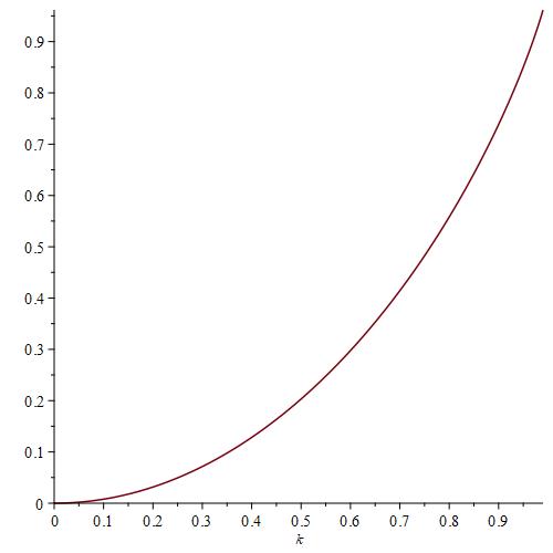
Figure 1: The graph of the function $g$

Here, we include several figures to conclude this note and visually demonstrate our method. We use the notation $x^{\prime}$, $y^{\prime}$, and $z^{\prime}$ to refer to the symmetries of our trajectories.

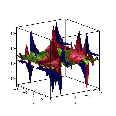
Figure 2: Local minimizer, in the case $\lambda=(\varphi,k)\in C_{1}$

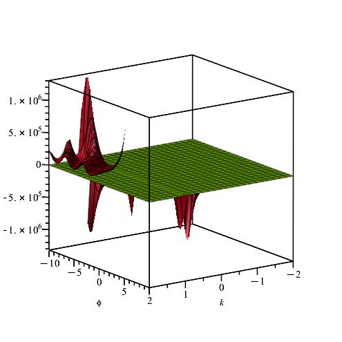
Figure 3: The trajectory’s symmetric

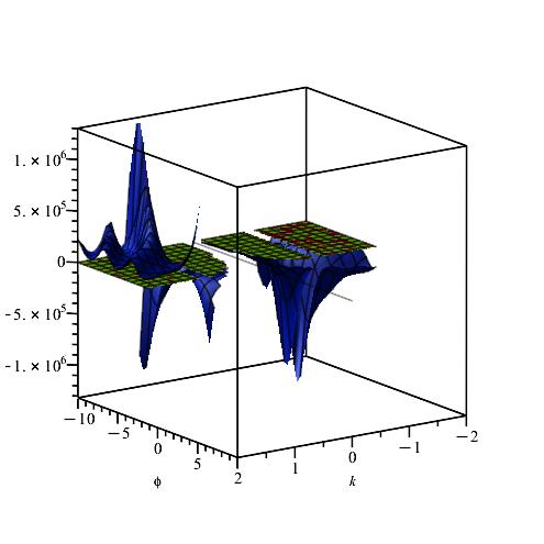
Figure 4: The trajectory $(x(t),y(t))$ and its symmetry, in the case $\lambda\in C_{1}$

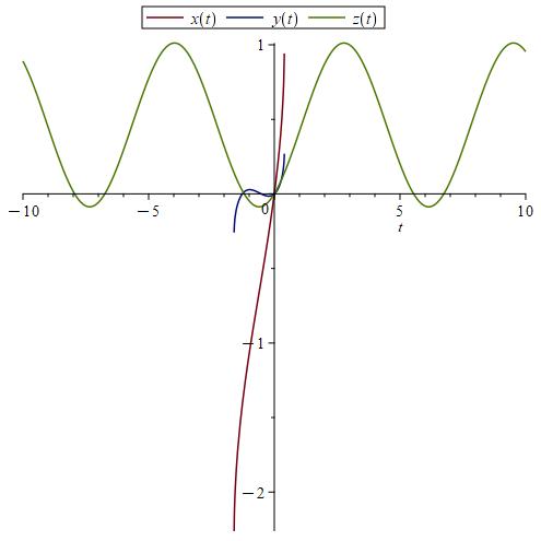
Figure 5: The local minimizer for numerical values, where $\lambda=(\varphi,k)\in C_{1}$.

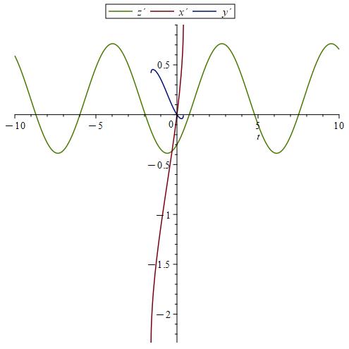
Figure 6: The trajectory’s symmetric for numerical values

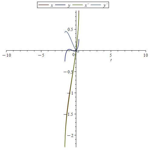
Figure 7: The trajectory $(x(t),y(t))$ and its symmetry for numerical values, where $\lambda\in C_{1}$.

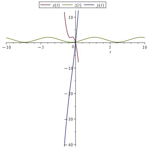
Figure 8: The local minimizer for numerical values, where $\lambda=(\varphi,k)\in C_{2}$.

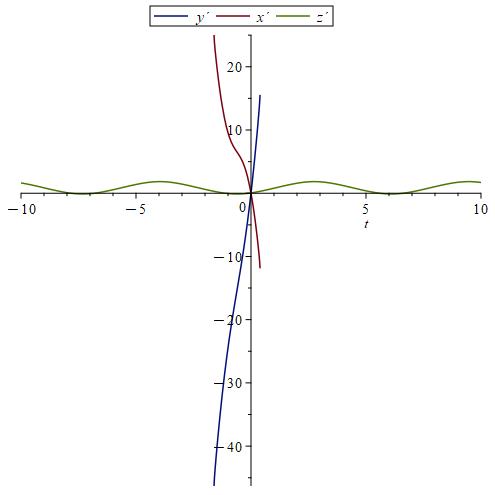
Figure 9: The trajectory’s symmetric for numerical values

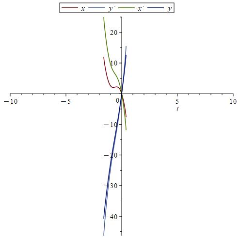
Figure 10: The trajectory $(x(t),y(t))$ and its symmetry for numerical value, where $\lambda\in C_{2}$

Upon analyzing the preceding figures, several key observations emerge. Figures 4, 4, and 4 provide a numerical-free overview of our trajectory and its symmetry, showcasing their intersections. Moving to Figure 7, we delve into a specific case where numerical values are assigned to $\varphi$ and $k$, allowing us to visualize the trajectories $x(t)$, $y(t)$, and $z(t)$. Figure 7 mirrors this setup, illustrating the symmetry of our trajectory using the same numerical values. Transitioning to the $(x,y)$ plane, Figure 7 displays the intersection between our trajectory and its symmetry, highlighting the absence of intersections for strictly positive times. This analytical approach is replicated for the second case, culminating in Figure 10, which reveals an intersection at a point closer to 0, with $k_{0}$ minimized.

References

• [1] A.A. Agrachev, D. Barilari, U. Boscain, A comprehensive introduction to sub-Riemannian geometry, Cambridge Studies in Advanced Mathematics, Cambridge University Press, 2019. https://doi.org/10.1017/9781108677325
• [2] Andrei Agrachev, Davide Barilari, Sub-Riemannian structures on 3D Lie groups, SISSA, Trieste, Italy and MIAN, Moscow, Russia, May 18, 2011.
• [3] Frank W. J, Daniel W, Ronald F, Ronald F, Charles W. Nist handbook of mathematical functions, National Institute of Standards and Technology 2010.
• [4] Igor Moiseev, Yuri L. Sachkov, Maxwell strata in sub-Riemannian problem on the group of motions of a plane, ESAIM: COCV 16 (2010) 380–399.
• [5] Jean Gallier, Jocelyn Quaintance, Notes on differential Geometry and Lie Groups [Lecture notes], 2016.
• [6] Peter J.Olver, Application of Lie Groups to Differential Equations
• [7] Velimir Jurdjevic, Optimal Control and Geometry: Integrable Systems, Cambridge Studies in Advanced Mathematics, Vol. 154, Cambridge University Press.
• [8] Yu. L. Sachkov, Complete description of the Maxwell strata in the generalized Dido problem, Sbornik: Mathematics 197:6 901–950, 2006.
• [9] Yu. L. Sachkov, The Maxwell set in the generalized Dido problem, 2006, RAS(DoM) and LMS, DOI: 10.1070/SM2006v197n04ABEH003771.
• [10] Yuri Sachkov, Introduction to Geometric Control, Springer Optimization and its Applications, Vol. 192.
• [11] Yasir Awais Butt, Sub-Riemannian Problem on Lie Group of Motions of Pseudo Euclidean Plane, 2015: 53-91.