Abstract

Understanding the structure of neural network loss surfaces, particularly the emergence of low-loss tunnels, is critical for advancing neural network theory and practice. In this paper, we propose a novel approach to directly embed loss tunnels into the loss landscape of neural networks. Exploring the properties of these loss tunnels offers new insights into their length and structure and sheds light on some common misconceptions. We then apply our approach to Bayesian neural networks, where we improve subspace inference by identifying pitfalls and proposing a more natural prior that better guides the sampling procedure.

1 INTRODUCTION AND RELATED WORK

Studying the emergence of lower-dimensional connected structures of low-loss in the high-dimensional loss landscape of neural networks is an important research direction fostering a better understanding of neural networks. Much of the literature in this area focuses on the connectedness of optimized networks. This property referred to as mode connectivity not only provides valuable insights into the landscape of hypotheses of a neural network, but can also be used to inform the optimization process (Ainsworth et al.,, 2023), improve sampling approaches in Bayesian neural networks (Izmailov et al.,, 2020; Dold et al.,, 2024), protect against adversarial attacks (Zhao et al.,, 2020), improve model averaging (Wortsman et al.,, 2022), and guide fine-tuning (Lubana et al.,, 2023).

Various forms of mode connectivity have therefore been studied. The most commonly investigated phenomenon is linear mode connectivity (Frankle et al.,, 2020; Entezari et al.,, 2022). Other connectivity hypotheses include linear layerwise connectivity (Adilova et al.,, 2024; Wortsman et al.,, 2022), quadratic (Lubana et al.,, 2023) or star-shaped connections (Sonthalia et al.,, 2024; Lin et al.,, 2024), geodesic mode connectivity (Tan et al.,, 2023), parametrized curves (Garipov et al.,, 2018), manifolds (Benton et al.,, 2021), and general minimum energy paths (Draxler et al.,, 2018). The latter, in particular, suggests that there is no “loss barrier” between modes if paths are constructed flexible enough. Current findings also suggest that shared invariances in networks induce connectivity of models, while the absence of (linear) connectivity implies dissimilar mechanisms (see, e.g., Lubana et al.,, 2023).

Apart from characterizing trained networks, some research also tries to improve and better understand mode connectivity by taking neural network properties into account. One of the most common approaches is to account for parameter space symmetries (Tatro et al.,, 2020; Entezari et al.,, 2022; Zhao et al.,, 2023). The initialization and type of architecture are further properties that were found to relate to the way loss valleys emerge (Benzing et al.,, 2022).

Direct Optimization of Subspaces  One promising approach tightly connected to mode connectivity is to embed a certain topological space into the loss landscape of the neural network and directly optimize this space. In contrast to the aforementioned literature, this changes the objective of the network training to find a region in the network’s parameter space in which relevant model hypotheses reside. Using a toy model representing high-dimensional intersecting wedges, Fort and Jastrzebski, (2019) were able to link the two objectives and reproduce some of the loss landscape properties of real neural networks. An alternative approach by Garipov et al., (2018) and Gotmare et al., (2018) is to directly optimize a path between two fixed modes in the actual network landscape.

Future Directions  While embedding a manifold of greater complexity into the loss landscape would be a natural extension of previous approaches, this also makes it harder to study and understand hypotheses within it. In contrast, loss tunnels or paths possess favorable properties that can be directly understood, and using a path does not limit the expressiveness of generated hypotheses in function space (Draxler et al.,, 2018). Despite being simpler than a complex manifold embedding, theoretical characteristics and the training of loss tunnels are not completely understood yet.

1.1 Our Contributions

This paper broadens the understanding of loss paths and tunnels by making the following contributions:
1. We propose a flexible method to directly embed loss tunnels into neural loss landscapes. Our approach can be trained with an arbitrary number of control points while also being modularly applicable to all types of neural networks. In contrast, existing approaches are more invasive in their adoption, e.g., requiring changes in the standard implementation of common layers.
2. We provide new insights into the nature of loss paths and tunnels, in particular their length, their optimization, benefits, and other important properties.
3. Using these insights and their implementation, we demonstrate how to advance subspace inference in Bayesian neural networks, an application that greatly benefits from such loss tunnels. For this, we also propose a matching and more intuitive prior that allows for better guidance of sampling procedures.

2 LOSS PATHS AND TUNNELS

2.1 Notation and Objective

In this work, we consider neural networks $f_{\bm{\theta}}:\mathcal{X}\to\mathcal{Y}$ mapping features $\mathbf{x}\in\mathcal{X}\subseteq\mathbb{R}^{p}$ to an outcome space $\mathcal{Y}\subseteq\mathbb{R}^{m}$. The network is parametrized with weights $\bm{\theta}\in\bm{\Theta}\subseteq\mathbb{R}^{D}$, where $D$ is typically very large and trained to minimize a loss function. In this work, we usually consider the loss function as a continuous function of the parameters: $\ell:\bm{\Theta}\to\mathcal{L}\subseteq\mathbb{R}$.

Objective  Our goal is to construct a lower-dimensional connected structure $\bm{\Phi}\subseteq\mathbb{R}^{K}$ of low loss in the high-dimensional loss surface $\bm{\Theta}$, where typically $K\ll D$. As discussed in Section 1, we will focus on paths and tunnels in this work. To formalize these structures, we define the following.

Definition 1 (Loss Path).

Let $\mathcal{T}:=[0,1]$. We call $\rho:\mathcal{T}\to\mathcal{L}$ a loss path if there exists a mapping $b:\mathcal{T}\to\bm{\Theta}$ such that $\rho:=\ell\circ b$ is a continuous function on $\mathcal{T}$.

In Definition 1, $b$ is used as the actual curve embedded into the neural network loss surface. While $\rho$ is a loss path in the sense that it yields loss values for a given “time” $t$, this is just a byproduct of the curve $b$ describing an ensemble of model parametrizations on $\mathcal{T}$, whose performance in turn is evaluated with $\ell$.

In contrast to a loss path, defined on $\mathcal{T}$, we consider a loss tunnel to be a multidimensional object.

Definition 2 (Loss Tunnel).

Let $\bm{\Xi}\subset\mathbb{R}^{K-1}$ be a compact space on $\mathbb{R}^{K-1}$. We call $\varrho:\mathcal{T}\times\bm{\Xi}\to\mathcal{L}$ a $K$-dimensional loss tunnel if for every $\bm{\xi}\in\bm{\Xi}$, $\varrho(\cdot,\bm{\xi}):\mathcal{T}\to\mathcal{L}$ defines a loss path on $\mathcal{T}$.

In other words, we obtain the loss tunnel by “lifting” a path into the product space and for every $t\in\mathcal{T}$ on the path, $\varrho(t,\cdot)$ describes a manifold (the ambient space) embedded in $\mathbb{R}^{K-1}$. Every combination of values $\bm{\xi}\in\bm{\Xi}$, in turn, defines a loss path in this tunnel.

Note that while we define loss paths and tunnels on compact spaces, this is merely to convey the idea of low-loss regions in $\bm{\Theta}$ similar to the idea of loss barriers, and there is typically no actual boundary in this space.

2.2 Path Optimization

Following Definition 2, the search for a loss tunnel naturally leads to finding a loss path first. A property shared by all existing path approaches is to define the initial and terminal point of the loss path. A common way to do this is to set $\bm{\theta}_{0}:=b(0)$ and $\bm{\theta}_{1}:=b(1)$, where $\bm{\theta}_{0},\bm{\theta}_{1}\in\bm{\Theta}$ represent two optimized neural networks solutions. Given these endpoints, a low-loss path can be constructed by finding a parameterized curve of constantly low-loss between those points (Draxler et al.,, 2018; Garipov et al.,, 2018). The hope is that this path contains functionally diverse, well-performing models.

As in previous approaches, we also use a parametrized regular curve $b$ to construct the loss path. We, however, opt for a more flexible way to learn this curve, not restricting ourselves to pre-defined endpoints, and thereby also constructing a method that can be adapted more flexibly (cf. Fig. 1). More specifically, we do not fix the endpoints of $b$, but instead, define $b$ based on $K+1$ control points $\bm{\theta}_{0},\ldots,\bm{\theta}_{K}\in\bm{\Theta}$ that can freely move in $\bm{\Theta}$. We then optimize this set of control points $\bm{\Lambda}:=\{\bm{\theta}_{0},\dots,\bm{\theta}_{K}\}$ that define the curve $b_{\bm{\Lambda}}$ by integrating over the current path loss

$$L(\bm{\Lambda}):=\int_{0}^{1}\rho_{\bm{\Lambda}}(t)dt=\int_{0}^{1}\ell(b_{\bm{\Lambda}}(t))dt.$$ (1)

While optimizing Eq. 1 corresponds to the optimization of a curve with constant “speed” $\|b_{\bm{\Lambda}}^{\prime}(t)\|$, an unrestricted approach would be to optimize over its expectation uniformly in the space $\bm{\Theta}$ (Garipov et al.,, 2018):

$$\tilde{L}(\bm{\Lambda}):=\int_{0}^{1}\!\!\ell(b_{\bm{\Lambda}}(t))\|b_{\bm{\Lambda}}^{\prime}(t)\|dt\cdot\left(\int_{0}^{1}\!\!\|b_{\bm{\Lambda}}^{\prime}(t)\|dt\right)^{-1}\!\!.$$ (2)

Since we use a parameterized regular curve, which has non-constant speed, we could reparameterize $t$ with the curve length $s$ through the relation $s=\int_{0}^{t}\|b_{\bm{\Lambda}}^{\prime}(u)\|du$ and sample $s\sim\text{Uniform}(0,\mathcal{S})$ instead of $t$ to convert Eq. 2 into Eq. 1. However, as also discussed in Garipov et al., (2018), this approach is computationally intractable due to the dependency of $s$ on $\bm{\Lambda}$. In particular, recovering $t$ from $s$ requires a root solver, which is in general not differentiable.

Importance Sampling  While previous approaches (Garipov et al.,, 2018; Izmailov et al.,, 2020; Dold et al.,, 2024) focused on implementing paths using the expectation over $t$ as in Eq. 1, a better understanding of loss paths also requires investigating the differences to an optimization using Eq. 2. To this end, we developed an importance sampling approach that allows optimizing Eq. 2. Details are given in the following section. As later results will demonstrate, there is negligible difference between the optimization of both objectives Eqs. 1 and 2. For this reason, we will thus focus on the objective in Eq. 1 in the following.

2.3 Practical Implementation

In practice, we suggest implementing the parametrized curve and, hence, the loss path in a way that allows easy adoption for any network architecture.

Path parametrization  A flexible and recently promoted approach is to use a Bézier curve (see, e.g., Garipov et al.,, 2018), which we define as

$$b_{\bm{\Lambda}}(t)=\sum_{k=0}^{K}\omega_{k}(t)\bm{\theta}_{k}:=\sum_{k=0}^{K}\binom{K}{k}(1-t)^{K-k}t^{k}\bm{\theta}_{k},$$ (3)

$t\in\mathcal{T}:=[0,1]$. Using $b_{\bm{\Lambda}}$, we define our loss path according to Definition 1 by setting $\rho:=\ell\circ b_{\bm{\Lambda}}$ (since Eq. 3 maps from $\mathcal{T}$ to $\bm{\Theta}$ and $\ell$ maps from $\bm{\Theta}$ to $\mathcal{L}$).

Loss computation  The advantage of a parametrized curve becomes evident when computing the path loss in Eq. 1. We do this by drawing $M$ samples from $t\sim U(0,1)$ in every forward pass and approximate the expectation $\int_{0}^{1}\ell(b_{\bm{\Lambda}}(t))dt=\mathbb{E}_{t\sim U(0,1)}[\ell(b_{\bm{\Lambda}}(t))]$ using Monte Carlo. In practice, using $M=1$ is often sufficient. Although increasing $M$ reduces gradient noise, we observed no significant performance improvements with larger values.

Model updates  Based on the previous loss computation discussion, we can derive the gradients for model updates for a given time point $t^{\ast}$ via the chain rule $\nabla_{\bm{\Lambda}}L:=\left\{\frac{\partial{L}}{\partial{\bm{\theta}_{0}}},\ldots,\frac{\partial{L}}{\partial{\bm{\theta}_{K}}}\right\}=\left\{\frac{\partial{L}}{\partial{b_{\bm{\Lambda}}(t^{\ast})}}\frac{\partial{b_{\bm{\Lambda}}(t^{\ast})}}{\partial{\bm{\theta}_{k}}}\right\}_{k\color[rgb]{0,0,0}=0,\ldots,K}$, where the first term $\frac{\partial{L}}{\partial{b_{\bm{\Lambda}}(t^{\ast})}}$ for each control point is the standard gradient $\nabla_{\bm{\vartheta}}\ell$ of the loss function $\ell$ for the given point $\bm{\vartheta}:=b_{\bm{\Lambda}}(t^{\ast})$ and the second term $\partial{b_{\bm{\Lambda}}(t^{\ast})}/{\partial{\bm{\theta}_{k}}}\equiv\omega_{k}(t^{\ast})$. Since the first term is independent of $k$, cached for all $K+1$ control points, and the second term is a scalar weighting, the model update can be performed inexpensively and efficiently using common auto-differentiation libraries. In particular, this routine does not require to build custom layer or network modules. Additionally, it can be straightforwardly combined with other inference approaches (such as last-layer Bayesian approximations), by only modifying a subset of model parameters using the weighting $\omega_{k}$. Decoupling the model architecture from parameter computations $\bm{\vartheta}$ also aligns well with modern functional deep learning frameworks such as JAX (Bradbury et al.,, 2018). We describe this implementation in Algorithm 1, exemplary using stochastic gradient descent (SGD).

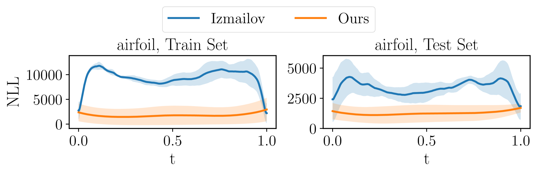
Figure 1: Negative log-likelihood (NLL; y-axis) along the path, comparing the method proposed in Izmailov et al., (2020) to our approach across five different data splits and initializations (shaded regions represent one std.dev.).

Integrating over $\mathcal{S}$  As discussed in the previous section, using Eq. 1 does not account for the “speed” of $b$ when computing its expectation. To directly optimize Eq. 2, we suggest using importance sampling by first drawing $t\sim U(0,1)$ and weighting the sample by $\|b_{\bm{\Lambda}}^{\prime}(t)\|\cdot\mathcal{S}^{-1}$, i.e., the speed at position $t$ divided by the total curve length, computed via numerical integration. Both terms are differentiable in this case. The resulting weight is again a scalar value multiplied with the gradient $\nabla_{\bm{\Lambda}}L$ as in the model updates. Since this introduces a computational overhead (the curve length $\mathcal{S}$ of $b$ must be recomputed in every update step), we investigate this adaption of Algorithm 1 in Section 4.5.

Algorithm 1 Path Finding

 initialize parameters $\bm{\Lambda}=\{\bm{\theta}_{0},\dots,\bm{\theta}_{K}\}$ randomly

 while validation loss still decreasing do

  for each batch $\mathcal{B}$ of training data $\mathcal{D}_{\text{train}}$ do

   Sample $t^{\ast}\sim U(0,1)$

   Compute $\bm{\vartheta}=b_{\bm{\Lambda}}(t^{\ast})$

   Compute $\ell(\bm{\vartheta})$ and gradients $\nabla_{\bm{\Lambda}}\mathcal{L}$.

   Update $\bm{\Lambda}$ using SGD

  end for

 end while

 return $\bm{\Lambda}$

2.4 Path Characteristics and Dynamics

For simple problems and exact optimization procedures, an optimal solution would be a collapsed curve with length $\mathcal{S}=0$ located at the global minimum of the loss landscape. Due to the complexity of the loss landscape and the stochastic optimization, we cannot expect the loss $\ell(b(t))$ to be constant along the path. For optimization using SGD on a simple loss function $\ell(\bm{\theta})$ over weights $\bm{\theta}$, it has recently been shown that the long-term probability $p_{i}$ of visiting a region $i$ with a local minimal loss follows a Boltzmann distribution $p_{i}\propto\exp\left(-\frac{E_{i}}{T}\right),$ where the energy term $E_{i}$ is related to the loss $\ell(\bm{\theta}_{i})$, and the temperature $T$ is related to the learning rate of SGD (Azizian et al.,, 2024). Boltzmann statistics describe a system where energetic terms (loss minimization) and entropic contributions (exploration due to noise) balance to form a stationary distribution. While the dynamics of Algorithm 1 are more complex compared to standard deep learning optimization, we still expect that the dynamics of the pathfinding result in two competing effects: an energetic term seeking the minimum of the loss functional $L(\bm{\Lambda})$ in Eq. 1, and an entropic term favoring typical configurations while disfavoring non-typical configurations such as entirely straight, elongated, or collapsed paths. This balance between energy minimization and entropy maximization prevents the path from collapsing to a single point and encourages the exploration of a diverse set of low-loss configurations along the path.

Simplified Entropic Model  To investigate the effect of the entropic contributions, we consider the case in which the path lies in an infinite region of constant loss so that the gradient of $\ell(\bm{\vartheta})$ vanishes. At first glance, this may seem like an overly strong assumption. However, in the long-time limit and without interventions during training, this assumption becomes reasonable if the loss landscape consists of minima surrounded by volumes of low-loss regions. Thus, to mimic the stochasticity in training, we replace the gradient $\nabla_{\bm{\Lambda}}L$ with a random component $\bm{\epsilon}\sim\mathcal{N}(0,\sigma^{2}I_{D})$ in the update of control point $\bm{\theta}_{k}$: $\bm{\theta}_{k}\leftarrow\bm{\theta}_{k}+\bm{\epsilon}\,\eta\omega_{k}(t^{\ast})$, where $\eta$ is the learning rate. This dynamic induces a diffusion process in which the relevant quantities exhibit a characteristic square-root dependence on the effective time constant, $\sqrt{n\,\eta^{2}\sigma^{2}}$, after $n$ update steps. This model is analogous to the dynamic of a polymer chain where the control points $\bm{\theta}_{k}$ represent the monomers or beads of the chain. The center of mass of the chain relative to its starting position diffuses as $\|\bar{\bm{\theta}}\|=\sqrt{n\,\eta^{2}\sigma^{2}}\cdot\sqrt{D}/(K+1)$, as shown by the dotted line in Panel (A) of Fig. 2. Also displayed are simulation results for $D=55$, selected as an intermediate value between $K=10$ and the maximum $K=80$ and different values of $\sigma$ averaged over 100 repetitions. While $\|\bar{\bm{\theta}}\|$ captures the overall movement of the chain, Panel (B) shows the end-to-end distance $R_{e}:=\left\|\bm{\theta}_{K}-\bm{\theta}_{0}\right\|$, which describes the relative positions between the monomers.

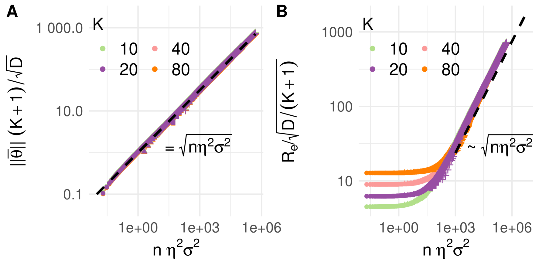
Figure 2: Scaling behavior of path characteristics. Panel (A) shows the center of mass $\|\bar{\bm{\theta}}\|$, and Panel (B) shows the end-to-end distance $R_{e}$, both following square-root scaling with the effective time constant. Symbols denote different values of $\sigma$: $\circ\,\sigma=0.1,\,\triangle\,\sigma=1,\,\square\,\sigma=5,\,\lozenge\,\sigma=10$, though some values are only partially visible due to overplotting.

After a transient period, $R_{e}$ is proportional to $\sqrt{n\;\eta^{2}\sigma^{2}\cdot}\sqrt{D/(K+1)}$. Similar scaling laws are observed for quantities like the squared radius of gyration $R_{g}^{2}=\frac{1}{K+1}\sum_{k=0}^{K}\|\bm{\theta}_{k}-\bar{\bm{\theta}}\|^{2}$, $\lambda_{K}=\sum_{k=0}^{K-1}\|\bm{\theta}_{k+1}-\bm{\theta}_{k}\|$ , and other characteristic quantities describing the chain (see Appendix A for more details). In polymer physics, characteristic lengths such as $R_{e}$, $R_{g}$ and $\|\bar{\bm{\theta}}\|$ exhibit universal scaling laws across various conditions, from dense melts to dilute solutions, as well as in simplified models (De Gennes,, 1979). In Section 4.1, we will investigate whether this also holds in neural networks.

2.5 Tunnel Embedding and Description

Having found a path of low loss, we now extend the path to a tunnel as described in Definition 2. This has various advantages, including better uncertainty quantification as discussed in Section 3.

Volume Lifting  In principle, there are several options to lift the path into a higher-dimensional space. For example, Izmailov et al., (2020); Dold et al., (2024) assume that every direction that the curve is taking reveals valuable insights. These directions are encoded by the subspace $\bm{\Phi}=\operatorname{span}(\bm{\Lambda})$. By defining $\bm{\Phi}$ this way, we discard the information of $b$ and instead work with the hyperplane in which $b$ resides. To perform inference or investigate model hypotheses, we therefore do not travel along $\mathcal{T}$, but instead define a projection matrix $\bm{\Pi}\in\mathbb{R}^{D\times K}$ mapping $\bm{\Pi}:\bm{\Phi}\to\bm{\Theta}$, i.e., taking an element $\bm{\varphi}\in\bm{\Phi}$ in this hyperplane (irrespective of $\mathcal{T}$) and map it back to a neural network weight $\bm{\theta}\in\bm{\Theta}$.

Tunnel Lifting  We propose tunnel over volume lifting because only a small portion of the volume in $\operatorname{span}(\bm{\Lambda})$ has a low loss. Instead, we construct a tunnel according to Definition 2 that preserves the time information of the original path when lifting it into a higher-dimensional space. More specifically, at each time point $t\in\mathcal{T}$, we can uniquely define the first dimension of a local orthogonal basis system by the tangent vector $\bm{\tau}(t)=\frac{db(t)}{{d}t}$. The $K-1$ other dimensions of the tunnel can be constructed by taking orthogonal directions $\bm{\kappa}_{k}\in\bm{\Phi}$ at each position $t$. Together, this defines a local orthogonal basis system $\bm{\Omega}(t):=\{\bm{\tau}(t),\bm{\kappa}_{1}(t),\ldots,\bm{\kappa}_{K-1}(t)\}$ and the rank-(K$-$1) vector bundle $\bm{\Xi}=\bigcup_{t\in\mathcal{T}}\operatorname{span}\left\{\bm{\kappa}_{1}(t),\ldots,\bm{\kappa}_{K-1}(t)\right\}$ defines the ambient space of the curve $b$.

Rotation Minimizing Frames  A natural way to construct the local orthogonal system $\bm{\Omega}$ is to use the Frenet–Serret frame (Frenet,, 1852; Serret,, 1851), where $\bm{\tau}(t)$ is the tangent vector, and subsequent normal, binormal and consecutive vectors are derived from $\bm{\tau}^{\prime}(t),\bm{\tau}^{\prime\prime}(t),\dots,\bm{\tau}^{(K-1)}(t)$. These derivatives are orthogonalized via a Gram-Schmidt process. This approach, however, has several drawbacks. First, the local coordinate system is undefined at any point $t$ where a derivative of $\bm{\tau}(t)$ is zero. Second, the larger $K$, the more expensive this construction will be due to the higher-order derivatives. Lastly, a sign flip in any curvature can cause the orthogonal system to flip, which is problematic for sampling routines presented later, relying on smooth transitions between different states.

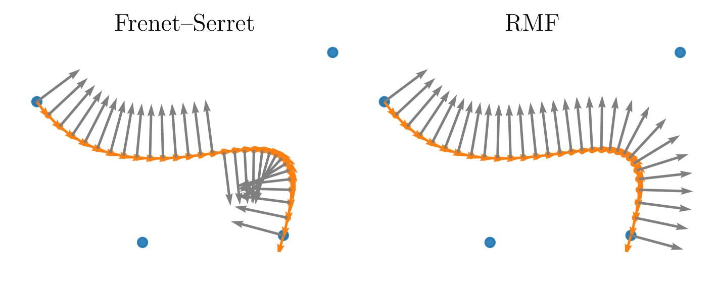
Figure 3: Frenet–Serret Frame (left) and our RMF implementation (right) on an exemplary 2D Bézier curve.

To avoid these issues, we instead use a Rotation Minimization Frame algorithm (RMF; see, e.g., Wang et al.,, 2008). RMF’s key idea is to minimize the rotational drift while maintaining a consistent frame orientation along the curve (cf. Fig. 3). For this, we construct a lookup table that starts with the initial orientation of the Frenet-Serret solution at $t=0$. The idea is to propagate this frame $\bm{\Omega}(0)$ without the tangent vector $\bm{\tau}$ along the curve and orthogonalize the frame at $t^{\ast}$ through the Gram-Schmidt process with the new tangent vector $\bm{\tau}(t^{\ast})$ and the previously stored frame. For this, we discretize $\mathcal{T}$ into a large number of discrete time points $0,\ldots,t_{i},\ldots,1$ and iterate through these until we find a point $t_{\text{cut}}$ where $\sphericalangle(\bm{\tau}(0),\bm{\tau}(t_{\text{cut}}))$ exceeds $45^{\circ}$. This implies that a sign flip can occur for any of the $\bm{\kappa}_{k}(t_{\text{cut}})$ directions. Hence, we add a new reference frame to our lookup table. This process is repeated until we reach $t=1$. For given $t^{\ast}$, we can then create the ambient space of the path by first finding $i:t_{i}\leq t^{\ast}<t_{i+1}$, and then initialize the Gram-Schmidt process using the tangent vector $\bm{\tau}(t^{\ast})$ and the previously stored frame.

2.6 Tunnel Symmetries

The idea of spanning a tunnel by orthogonal directions is also desirable from a permutation invariance point of view. More specifically, we can avoid permutation symmetries, which are known to dramatically increase the number of low-loss areas in neural landscapes and hinder mode connectivity (Pittorino et al.,, 2022). While the control points themselves are $\mathbb{P}$-almost surely permutation symmetry-free, the path might still contain permutations and thus lead to reduced functional diversity in $f_{\bm{\theta}}$.

Theorem 1 (informal).

If each $\bm{\theta}\in\bm{\Lambda}$ is permutation symmetry-free, an $\epsilon$-tube, $\epsilon>0$, exists around the path $b_{\bm{\Lambda}}$ that also contains no permutation symmetries.

In other words, if the optimized path $b$ is permutation symmetry-free, then the constructed tunnel will also contain no permutation symmetries in the path’s vicinity. A formal statement and proof are given in Appendix B. To ensure that models in $\bm{\Lambda}$ are permutation-free in each layer, one option is to sort the biases in each layer (Pourzanjani et al.,, 2017). In our experiments, we observe that even without this explicit enforcement, functional diversity along the path is usually obtained and the optimization of $b$ is not prone to get stuck in permutation invariances (cf. Section D.5). The nearly identical performances of the subspace approach with and without bias sorting in our further experiments suggest that the path itself, without explicit adjustments, consists of permutation-free solutions (cf. Section D.5).

3 ADVANCING SUBSPACE INFERENCE

After optimizing $b$ as in Algorithm 1, sampling values from this curve $b$ will likely yield well-performing models since these define linear combinations of the $K+1$ optimized models $\bm{\theta}_{k}$. The constructed tunnels, in contrast, allow to also traverse to directions orthogonal to the curve and better explore the variability in $\bm{\theta}_{k}$.

Subspace Inference  The first to combine ideas of subspace construction and uncertainty quantification were Izmailov et al., (2020). Building on the work of Garipov et al., (2018), Izmailov et al., (2020) proposed to use three models of a parameterized curve to span a plane $\bm{\Phi}\subseteq\mathbb{R}^{2}$ (i.e., do a volume lifting) and run MCMC-based approaches in this subspace. Analogously to this idea, we study the use of the previously proposed tunnels to guide MCMC-samplers through the loss landscape and the choice of a meaningful prior.

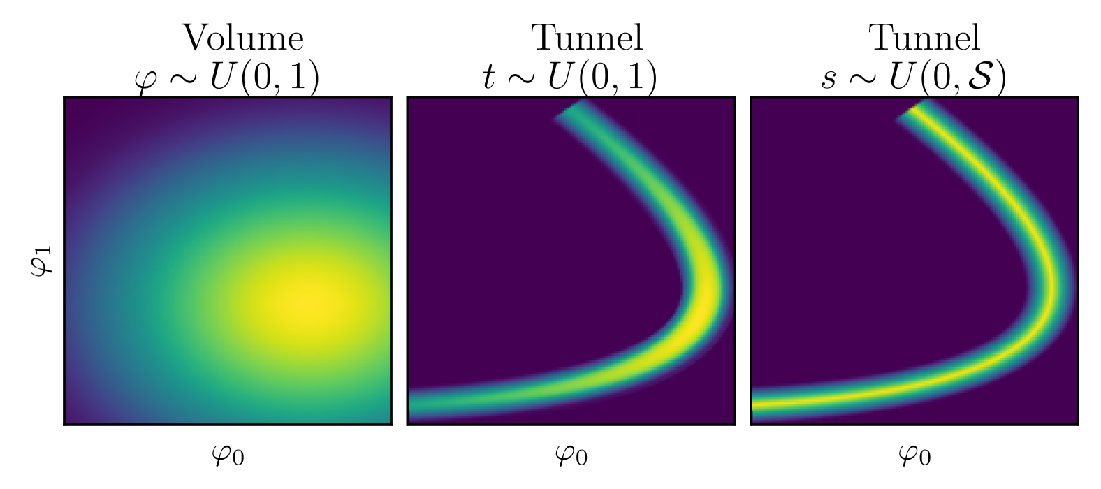
Figure 4: Comparison of a prior in the “volume space” (left), in the tunnel space with a uniform prior on $t$ (center) and in the tunnel space with adjusted prior through $s\sim U(0,\mathcal{S})$ (right).

Tunnel Priors  The most common prior assumption in Bayesian deep learning is an isotropic standard normal prior. While Izmailov et al., (2020) argue that the prior is not crucial for good performance if “sufficiently diffuse”, this does not hold in the aforementioned tunnels. More specifically, while using $\bm{\varphi}\sim\mathcal{N}(0,\bm{I}_{K})$ over $\bm{\Phi}$ might yield reasonable results for an unstructured subspace, this prior ignores the embedded structures of $\bm{\Phi}$ in the case its construction follows the previous tunnel approach. Ideally, we would want high prior probability for areas close to the center loss path spanning the tunnel, and gradually decreasing probability density towards the “boundaries” of the tunnel (cf. Fig. 4).
Tunnel prior in $t$: Using prior $t\sim U(0,1)$ and $\bm{\xi}\sim N(0,\sigma^{2}\bm{I}_{D})$ solves this problem. However, the tunnel prior with uniform distribution in $t$ suffers from being stretched or squeezed in $\bm{\Phi}$ due to the varying traversal speed $\|\bm{\tau}(t)\|$. Additionally, bendings along the path increase the prior density inside and decrease it outside the curve (center image in  Fig. 4).
Tunnel prior in $s$: To correct for this effect, we adjust the prior by incorporating the volume change with the Jacobian determinant between $\bm{\Phi}$ and $(\mathcal{T}\times\bm{\Xi})$ with $\log|\det({\partial g(t,\bm{\xi})}/{\partial t,\bm{\xi}})|$, where $g\colon(\mathcal{T}\times\bm{\Xi})\to\bm{\Phi}$ is the mapping from the tunnel into the subspace. While the adjusted prior is only known up to a normalization constant, this is sufficient for the subsequent sampling procedure. To further reduce the computational complexity of the Jacobian determinant associated with increasing $K$, we only adjust for the different speeds of $\|\bm{\tau}(t)\|$ through sampling $s\sim U(0,\mathcal{S})$ instead of $t\sim U(0,1)$ as in the right image of Fig. 4.

4 NUMERICAL EXPERIMENTS

We now empirically investigate loss paths and tunnels, and validate previous theoretical findings. For fundamental properties, we generate synthetic data to ensure a controlled environment. Performance results are obtained on common benchmark datasets. For further results and details see Appendices D and E.

4.1 Scaling Behavior in Loss Landscapes

Next, we investigate whether there are phases in the complex dynamics of the path (cf. Section 2.4) where the purely entropic nature of the diffusion process is preserved or if energetic terms become dominant. To this end, we use the scaling laws implied by our previous model assumption as a diagnostic tool.

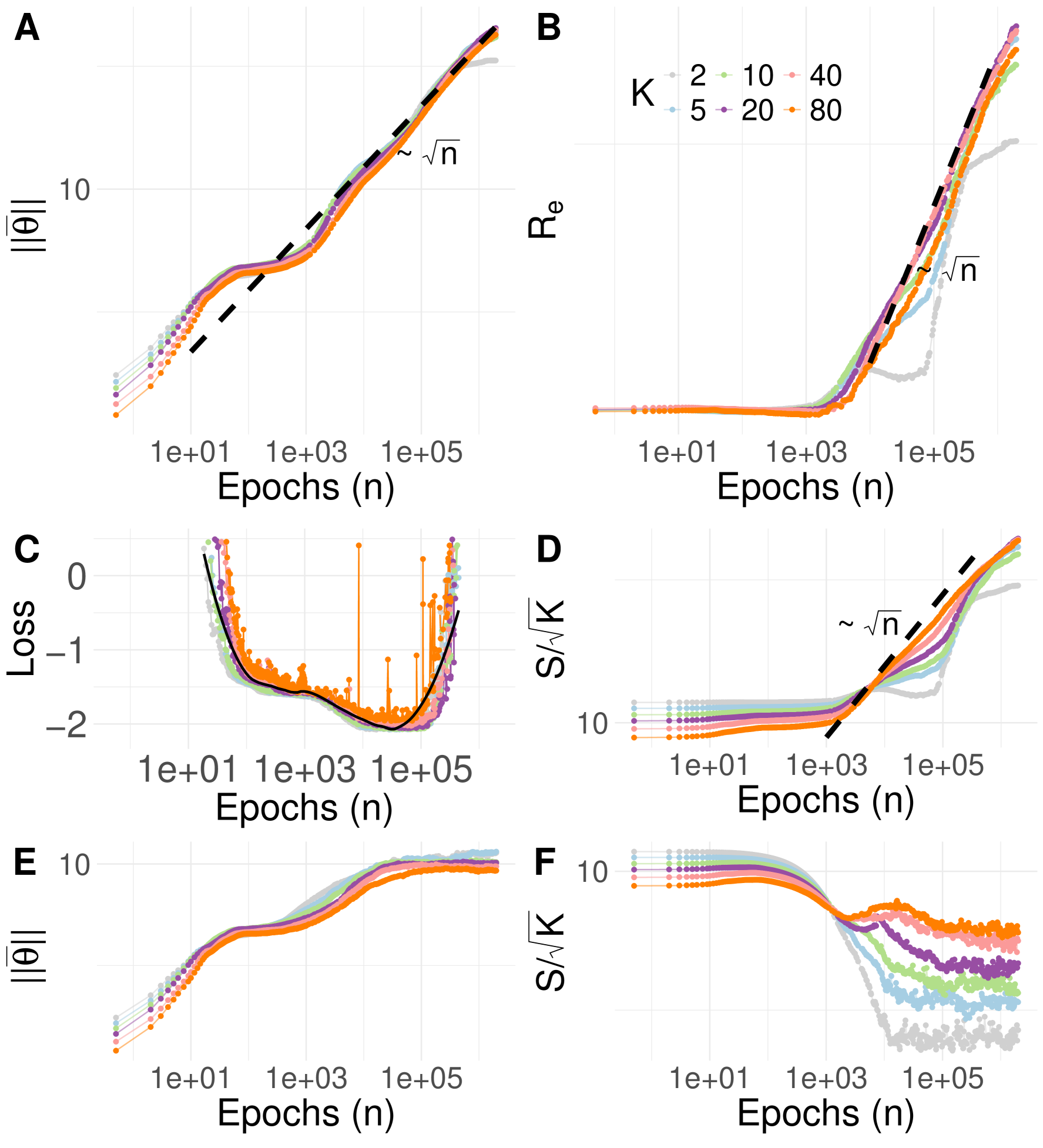
Figure 5: Corresponding to Fig. 2, Panels A and B show $\|\bar{\bm{\theta}}\|$ and the end-to-end distance ($R_{e}$), respectively. Panel C presents the training loss function, while Panel D depicts the Bézier curve length ($\mathcal{S}$). The lower panels include a weight decay of 0.1, which restricts free diffusion.

Results  In Fig. 5 we summarize our experiment. We expect to observe an initial drift phase where the entire chain moves within the loss landscape toward a minimal region. Looking at the loss function in Panel C, we observe a plateau reached after approximately $500$ epochs. This behavior is also reflected in the magnitude of the gradient $\sum_{k=0}^{K}||\nabla{\partial L}/{\partial\bm{\theta}_{k}}||_{2}$ (cf. Fig. 12). From around 2000 epochs onward, we see the typical behavior of $\sqrt{n}$-growth in length quantities B) and D), which corresponds to the free diffusion model, as predicted in Section 2.4. As shown in Panel D, the curve length $\mathcal{S}$ also exhibits this dependency. This is consistent with the relationship $R_{e}\leq\mathcal{S}\leq\lambda_{K}$. By analogy to polymers, we expect further that all quantities related to the distances between monomers share a similar diffusion time constant, which we also observed for other measures like $R_{g}$ (see Appendix A).

From around $10^{5}$ epochs, we observe instabilities in the optimization process, while the scaling laws still hold. Thus, it is recommended to stop training before reaching this regime. In our applications, these instabilities were not problematic, as early stopping based on validation data consistently halted training before reaching this point. The free diffusion behavior changes when external potentials are applied, as these introduce forces that can significantly alter the dynamics of the system. Weight decay, for example, can be viewed as adding a quadratic penalty term $\frac{\lambda}{2}\|\bm{\theta}\|^{2}$ to the loss function, effectively creating a harmonic potential that pulls weights towards zero. This additional potential restricts the free diffusion, and as shown in the lower panels of Fig. 5, can halt the unrestricted movement of the weights or, in extreme cases, cause the curve length to collapse.

4.2 Volume vs. Tunnel Sampling

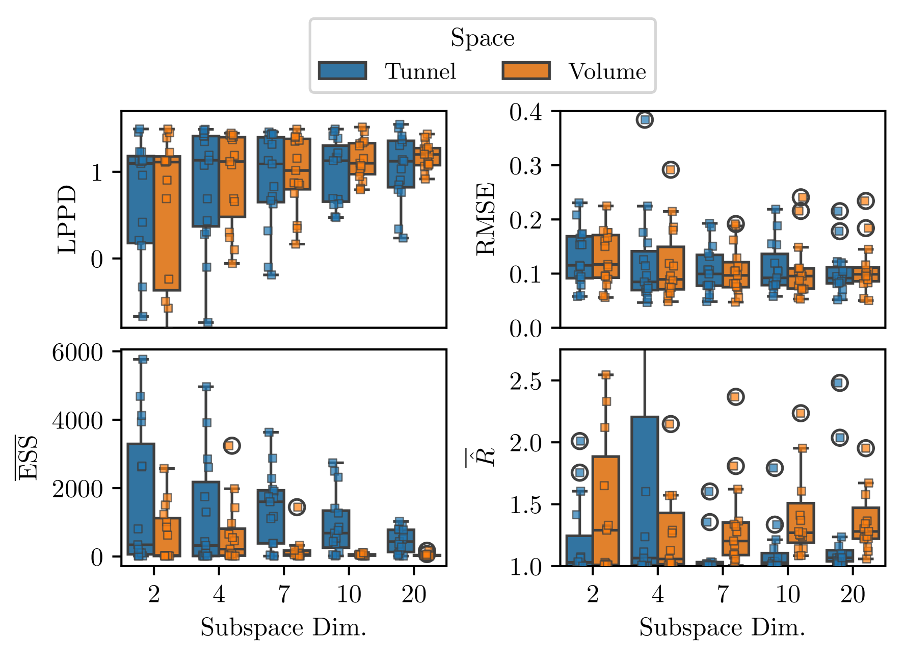
Figure 6: Performance (upper row) and sampling (bottom row) metrics on the synthetic dataset over 15 repetitions. Small square points show the underlying data. ESS and ${\hat{R}}$ are averages over all parameters.

To investigate the influence of our approach, we perform the tunnel lifting with its tunnel prior on the simulated data (cf. Section D.1.1) and investigate the performance of the sampling procedure on test data as well as the quality of the obtained samples. We compare this to the volume lifting approach using the log posterior predictive density (LPPD), root mean squared error (RMSE), averaged Effective Sample Size (ESS), and the averaged Gelman-Rubin $\hat{R}$ metric.

Results  Fig. 6 visualizes the performance comparison between the two lifting approaches. While there is little change between the two spaces in prediction performance, we see a notable trend in performance improvement for larger subspace dimensions, particularly in the LPPD, and to a lesser extent in the RMSE. As $K$ increases, it also becomes more likely to obtain better generalizing models, since the worst performance across repetitions improves. Furthermore, the tunnel approach shows notably better average ESS and $\hat{R}$ values, while there is a clear decline in the number of effective samples when using the volume approach. This supports the hypothesis that our tunnel construction improves the problem’s conditioning.

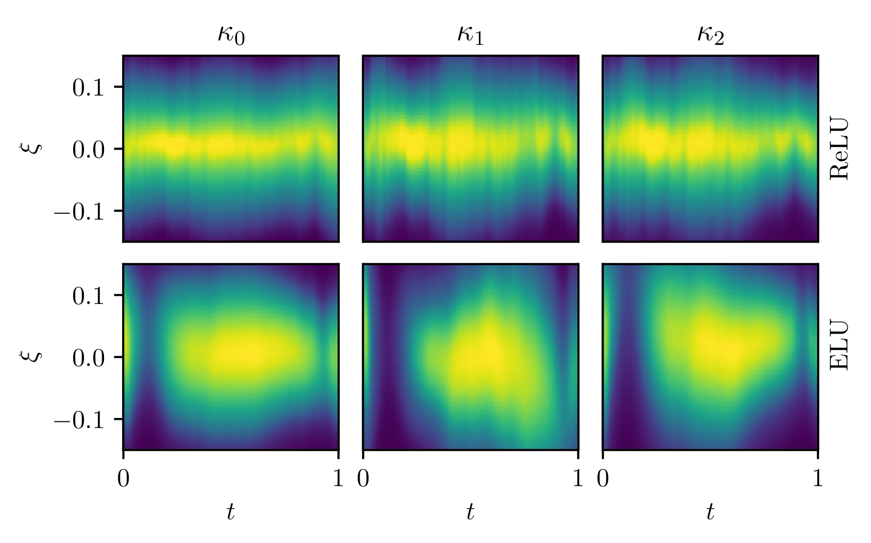
Figure 7: First four dimensions of the tunnel space (x-axis and different columns) for different activation functions (different rows) on the yacht dataset with remaining $\bm{\xi}$-dimensions set to zero. The x-axis represents the $t$-dimension, and the y-axis is one $\bm{\xi}$-dimension. The color represents the unnormalized log posterior value.

Table 1: Performance comparisons across different methods (columns) and datasets (rows) for the LPPD and RMSE metric. The method closest to the MCMC gold standard is highlighted in bold.

		MCMC	DE	LA	ModeCon	Tunnel-$2$	Tunnel-$20$
LPPD ($\uparrow$)	airfoil	0.67 ± 0.04	-1.09 ± 0.05	-3.05 ± 0.16	0.09 ± 0.05	0.25 ± 0.09	0.34 ± 0.04
	bikesharing	0.28 ± 0.04	-0.94 ± 0.03	-2.83 ± 0.11	0.02 ± 0.03	0.12 ± 0.04	0.14 ± 0.03
	concrete	0.09 ± 0.18	-0.94 ± 0.07	-2.99 ± 0.27	-0.29 ± 0.14	-0.08 ± 0.05	-0.04 ± 0.09
	energy	2.18 ± 0.07	-0.91 ± 0.07	-2.90 ± 0.19	1.59 ± 0.05	1.74 ± 0.14	1.70 ± 0.28
	yacht	2.90 ± 0.19	-0.91 ± 0.14	-2.91 ± 0.63	1.33 ± 0.80	0.75 ± 3.01	1.33 ± 1.75
RMSE ($\downarrow$)	airfoil	0.15 ± 0.02	0.30 ± 0.02	0.27 ± 0.03	0.22 ± 0.01	0.19 ± 0.01	0.18 ± 0.01
	bikesharing	0.21 ± 0.01	0.26 ± 0.01	0.25 ± 0.01	0.25 ± 0.01	0.23 ± 0.01	0.23 ± 0.01
	concrete	0.25 ± 0.02	0.31 ± 0.01	0.44 ± 0.03	0.31 ± 0.02	0.30 ± 0.02	0.28 ± 0.02
	energy	0.03 ± 0.00	0.07 ± 0.01	0.06 ± 0.01	0.05 ± 0.00	0.04 ± 0.01	0.05 ± 0.01
	yacht	0.04 ± 0.01	0.13 ± 0.03	0.13 ± 0.04	0.06 ± 0.01	0.05 ± 0.01	0.04 ± 0.01

4.3 Tunnel Smoothness

Next, we investigate how the tunnel is evolving across different dimensions and different activation functions. The latter was found to have a notable influence on the subspace’s smoothness, potentially affecting the sampling efficiency. For this, we visualize the first four dimensions of the created tunnels together with the unnormalized log posterior values on the yacht dataset. The results (cf. Fig. 7) confirm that the tunnel for ReLU networks is coarser compared to ELU activation, likely due to the non-continuously differentiable nature of ReLU. ELU, on the other hand, exhibits smoother transitions, although the multimodal structure observed in Fig. 7 can hinder efficient sampling.

4.4 Regression Benchmarks

To analyze the performance of sampling-based tunnel inference, we extend the benchmark setup from Sommer et al., (2024), with a Bayesian neural network in a homoscedastic regression setting with three hidden layers, each with 16 neurons and ReLU-activation using an MCMC-based solution for the UCI benchmark datasets airfoil, bikesharing, concrete, energy, and yacht. We take their MCMC method based on NUTS as the gold standard and compare it with the mode connectivity (ModeCon) method from Izmailov et al., (2020), and our tunnel (Tunnel-$K$) approach. We further use Laplace approximation (LA; Daxberger et al.,, 2021) and a non-Bayesian deep ensemble (DE; Lakshminarayanan et al.,, 2017) as baselines. We use five data splits to estimate the standard deviation in the performance metrics.

Results  Based on the results in Table 1, our method consistently outperforms both DE and LA in terms of LPPD. Furthermore, we observe improvements over ModeCon, except for the yacht dataset. More importantly, increasing our tunnel’s dimension $K$ leads to improvements in most cases. This suggests that the loss surface exhibits additional complexity that only a higher-dimensional subspace can capture. A similar trend holds for RMSE values, where we outperform LA, DE, and ModeCon, albeit by a smaller margin.

4.5 MNIST

To demonstrate that our method is also applicable to other network architectures, we run our tunnel-based approach using our tunnel-prior for the MNIST dataset to investigate whether a more complex model architecture might benefit from a “larger” tunnel. We investigate a subspace dimension of $K\in\{2,5,10,20\}$ and again report LPPD values in addition to the accuracy on MNIST’s standard test dataset. By altering the path optimization as discussed in Section 2.2, we also investigate the difference in optimizing Eq. 1 or Eq. 2. As a baseline, we use LA.

Results  Fig. 8 depicts the results, showing an increase in LPPD for an increase in subspace dimension. However, an increase in dimension is not necessarily beneficial for prediction accuracy (ACC) as the tunnel dimensions expand away from the path of well-performing ensemble members, confirmed by the empirical results. Additionally, there is little to no noticeable difference between the sampling procedures (indicated by different colors) used to approximate the integral over the loss path. Compared to the LA baseline, subspace inference yields notably better performance in terms of LPPD but does not surpass LA in its accuracy. Further analysis suggests a trade-off between optimizing LPPD and accuracy, which can, for example, be adjusted using the temperature parameter (cf. Section E.3). This again highlights the natural property of the tunnel as a way to capture surrounding uncertainty in parameter space while deviating from the path of high-performing models.

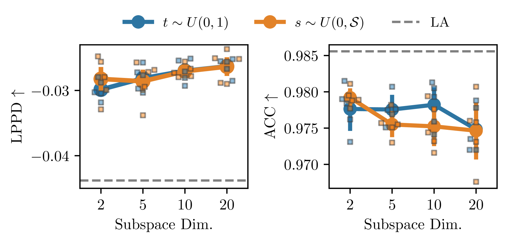
Figure 8: Mean performance on MNIST (with error bars visualizing standard error over five different folds) using different sampling approaches to optimize the path (color) and subspace dimensions $K$ (x-axis). The dashed line shows results obtained with Laplace Approximation (LA).

5 CONCLUSION

In this work, we formalized and analyzed loss paths and loss tunnels in neural network loss landscapes. Drawing on a range of theoretical and empirical perspectives, we offer new insights into these landscapes and discuss various properties relevant when resorting to such approaches. Empirical performance results suggest that the creation of paths and tunnels can be beneficial for sample-based inference.

Limitations and Future Work  Our study focused on loss tunnels constructed along a pre-defined optimized path. Directly embedding tunnels into neural landscapes by, e.g., pre-defining tunnel properties a priori is a potentially interesting future direction that would allow the direct optimization of such a tunnel.

Acknowledgements

We thank the reviewers, Beate Sick and Georg Umlauf, for their valuable feedback and fruitful discussions. This work was supported by the Carl-Zeiss-Stiftung in the project ”DeepCarbPlanner” (grant no. P2021-08-007).

SUPPLEMENTARY MATERIAL

Appendix A Derivation of Scaling Laws and Further Results

In the absence of a loss gradient (i.e., in a flat loss landscape), the updates to the control points $\bm{\theta}_{k}$ are dominated by the noise term $\bm{\epsilon}$. The change in $\bm{\theta}_{k}$ for a single update step is given by:

$$\Delta\bm{\theta}_{k}=\bm{\theta}^{(n+1)}_{k}-\bm{\theta}^{(n)}_{k}=\eta\,\bm{\epsilon}\,\binom{K}{k}{t^{\ast}}^{k}(1-t^{\ast})^{K-k}.$$ (4)

The dependence on $K$ arises due to how the noise in the updates is distributed among the control points of the Bézier curve. In the update rule, the factors $\binom{K}{k}t^{\ast}{}^{k}(1-t^{\ast})^{K-k}$ correspond to the weights of a binomial distribution, which are sharply peaked around $k=Kt^{\ast}$ for large $K$. This means that at each time, only a subset of control points near $k=Kt^{\ast}$ receive significant updates, while others receive negligible updates.

A.1 Effect on the Center of Mass

The center of mass of the control points is defined by:

$$\bar{\bm{\theta}}=\frac{1}{K+1}\sum_{k=0}^{K}\bm{\theta}_{k}.$$ (5)

The change in the center of mass $\bar{\bm{\theta}}$ from one time step to the next can be expressed as:

$$\Delta\bar{\bm{\theta}}=\bar{\bm{\theta}}^{(n+1)}-\bar{\bm{\theta}}^{(n)}=\frac{1}{K+1}\sum_{k=0}^{K}\Delta\bm{\theta}_{k}=\frac{\eta\,\bm{\epsilon}}{K+1}\sum_{k=0}^{K}\binom{K}{k}{t^{\ast}}^{k}(1-t^{\ast})^{K-k}=\frac{\eta\,\bm{\epsilon}}{K+1},$$ (6)

since the sum over the binomial coefficients equals 1. If we start with $\bar{\bm{\theta}}^{0}=0$, the center of mass after $n$ steps is given by adding up Eq. 6 $n$ times, yielding

$$\bar{\bm{\theta}}^{(n)}=\frac{n\eta}{K+1}\sum_{i=1}^{n}{\bm{\epsilon}}.$$ (7)

From this random process, we can calculate the expectation and variance. Assuming $\bm{\epsilon}\sim\mathcal{N}(0,\sigma\mathbf{I}_{D})$, the expectation $\mathbb{E}(\bar{\bm{\theta}}_{n})=0$ and square root of the variance is:

$$\|\bar{\bm{\theta}}\|=\sqrt{\operatorname{Var}\left(\bar{\bm{\theta}}\right)}=\sqrt{n\eta^{2}\sigma^{2}}\cdot\frac{\sqrt{D}}{(K+1)}.$$ (8)

Fig. 9 shows the near-perfect agreement between the simulation results of the distance of the center of mass from its origin and the theoretical result (solid lines) of Eq. 8.

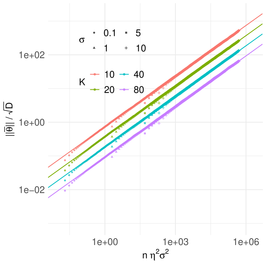
Figure 9: Center of mass comparison of Eq. 8 with simulation results for various $K$s (color) and different values of added noise $\sigma$ (shapes) using starting value $\bar{\bm{\theta}}^{(0)}=0$.

A.2 Additional Geometric Quantities and Scaling Laws

To better understand the structure and dynamics of the control points $\bm{\theta}_{k}$ in our model, we analyze several geometric quantities analogous to those in polymer physics. These quantities help us quantify how the control points spread and move over time due to stochastic updates.

Scaling with respect to $n$ and $D$

For all geometric quantities discussed, the scaling with respect to the dimensionality $D$ and the number of update steps $n$ is identical. Specifically, they all scale proportionally to $\sqrt{n}$ and $\sqrt{D}$. This is because the updates of the control points are driven by a random walk in a $D$-dimensional space. Over $n$ steps, the expected displacement in a random walk grows like $\sqrt{n}$ due to the accumulation of variance from independent random steps. Similarly, in $D$ dimensions, each independent component contributes to the total displacement, leading to a scaling of $\sqrt{D}$ for the magnitude of the displacement.

Scaling with Respect to $K$

To understand the scaling with respect to the number of control points $K$, we consider the average end-to-end distance after $n$ steps:

$$R_{e}^{2}=\mathbb{E}\left[\left\|\bm{\theta}^{(n)}_{K}-\bm{\theta}^{(n)}_{0}\right\|^{2}\right].$$

Using the update rule for the control points (from Eq. 4), the position of control point $\bm{\theta}^{(n)}_{k}$ after $n$ steps is

$$\bm{\theta}^{(n)}_{k}=\bm{\theta}^{(0)}_{k}+\sum_{i=1}^{n}\Delta\bm{\theta}^{(i)}_{k},$$

where $\bm{\theta}^{(0)}_{k}$ is the initial position, and $\Delta\bm{\theta}^{(i)}_{k}$ is the update at time step $i$, given by

$$\Delta\bm{\theta}^{(i)}_{k}=\eta\,\bm{\epsilon}^{(i)}\,c_{k},$$

with $c_{k}=\binom{K}{k}{t^{\ast}}^{k}(1-t^{\ast})^{K-k}$ . Assuming the initial positions are zero or negligible for long times, the difference between the positions of control points $k=K$ and $k=0$ after n steps simplifies to:

$$\bm{\theta}^{(n)}_{K}-\bm{\theta}^{(n)}_{0}=\sum_{i=1}^{n}\left(\Delta\bm{\theta}^{(i)}_{K}-\Delta\bm{\theta}^{(i)}_{0}\right)=\eta\,(c_{K}-c_{0})\sum_{i=1}^{n}\bm{\epsilon}^{(i)}.$$

To calculate the expectation, we note that there are two independent terms we have to average. First, the random noise $\bm{\epsilon}$ introducing a random walk for which the expectation of $\left\|\sum_{i=1}^{n}\bm{\epsilon}^{(i)}\right\|^{2}$ is $nD\sigma^{2}$. Second, the averaging over the uniform $t^{\star}\sim U(0,1)$ yields

$$\mathbb{E}_{t}{{}^{\star}}\left[\left\|c_{K}-c_{0}\right\|^{2}\right]=\int_{0}^{1}(t^{K}-(1-t)^{K})^{2}\;dt\propto\frac{1}{K}\text{for}K\gg 1.$$

Thus, the expected squared end-to-end distance scales as

$$R_{e}^{2}\propto\eta^{2}\sigma^{2}n\frac{D}{K+1}.$$ (9)

Typical Length $\delta$

Instead of relying on exact derivations, we employ informal scaling arguments to derive the following quantities, which are then verified numerically. In scaling theory, the typical length represents the characteristic length scale of the problem (De Gennes,, 1979). In our case, the typical length scale $\delta$ of the polymer chain can be formally interpreted as the average distance between the control vectors. Viewing the chain of control points as a random walk of $K$ steps, the end-to-end distance relates to the typical length between control points:

$$R_{e}\propto\sqrt{K}\delta.$$

Solving for $\delta$ (ignoring potentials differences between $K$ and $K+1$), we get

$$\delta\propto\frac{\eta\,\sigma\,\sqrt{nD}}{K}.$$

Total Length $\lambda_{K}$

The total length of the chain is $K$ times the typical length

$$\lambda_{K}=\sum_{k=0}^{K-1}\left\|\bm{\theta}_{k+1}-\bm{\theta}_{k}\right\|\approx K\delta\propto\eta\,\sigma\,\sqrt{nD}.$$

This shows that $\lambda_{K}$ is independent of $K$.

Radius of Gyration $R_{g}$

The radius of gyration measures the average squared distance of the control points from their center of mass:

$$R_{g}^{2}=\frac{1}{K+1}\sum_{k=0}^{K}\left\|\bm{\theta}_{k}-\bar{\bm{\theta}}\right\|^{2}.$$

A scaling argument for the radius of gyration is as follows: if we increase the size of the system by a certain factor, the radius of gyration should increase by the same factor. Thus, the radius of gyration should scale like the typical length $\delta$. In a random walk with $K$ steps, $R_{g}$, which measures the spread of the chain’s points around its center of mass, exhibits the same dependence on $K$ as the end-to-end distance $R_{e}$. Therefore, we have $R_{g}\propto\delta\sqrt{K}$. For a more detailed derivation, see De Gennes, (1979). This scaling leads to the following expression:

$$R_{g}\propto\sqrt{n\,\eta^{2}\,\sigma^{2}}\cdot\sqrt{\frac{D}{K+1}}.$$

Note that, when using scaling laws, we cannot distinguish between $K$ and $K+1$ precisely; however, we choose $K+1$ for better alignment with the observations from the subsequent simulation study.

A.3 Simulation Study

We conducted a comprehensive simulation study to validate the derived scaling laws and analyze the geometric properties of loss paths in neural networks. The study systematically varies three key parameters: the number of control points ($K$), the dimensionality of the space ($D$), and the noise amplitude ($\sigma$). Each combination of values is simulated over a large number of update steps $n$ and averaged over 100 repetitions, yielding approximately 60,000 data points. Despite variations in $K$, $D$, and $\sigma$, all quantities collapse onto a single curve when plotted against the effective time parameter $n\eta^{2}\sigma^{2}$ for large values of it. This is shown in Fig. 10, confirming the universal nature of the scaling laws, which are summarized in column ’Simplified Model Scaling’ in Table 2.

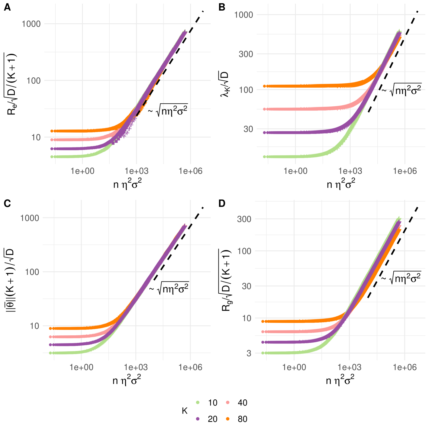
Figure 10: Simulation study and scaling laws: subplot (A) $R_{e}$, (B) $\lambda_{K}$, (C) $\left\|\bar{\bm{\theta}}\right\|$ without substracting starting point (D) $R_{g}$. Quantities in A-D plotted to show scaling behavior.

A.4 Comparison with Path Optimization

This subsection compares our approach to path optimization methods using Algorithm 1, expanding on the main results. Figure 11 illustrates the metrics $R_{g}$ and $\lambda_{K}$, which are not included in Fig. 5. We can observe the scaling behavior with respect to $\sqrt{n}$ for large epochs $n$. Table 2 summarizes and compares our theoretical findings to the scaling observed in our simplified model.

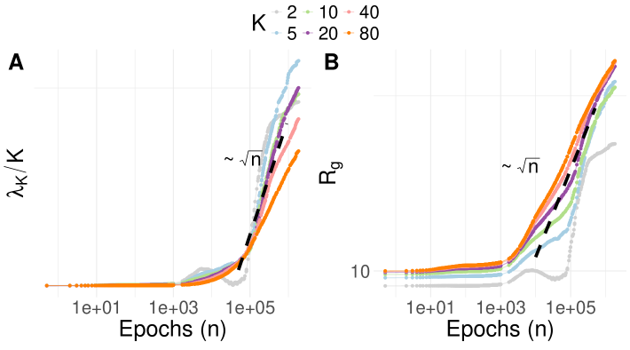
Figure 11: Additional results to Fig. 5 for the path optimization with zero weight decay.

While the scaling with respect to the time constant appears to be approximately $\propto\sqrt{n}$, we observe notable deviations in the scaling with $K$ and $D$. These differences are expected due to the complex dynamics introduced by the Adam optimizer.

Quantity	Simplified Model Scaling	Simulation Scaling
Radius of Gyration $R_{g}$	$R_{g}\propto\sqrt{n\,\eta^{2}\sigma_{n}^{2}}\cdot\sqrt{\frac{D}{K+1}}$	$R_{g}\propto\sqrt{n}$
End-to-End Distance $R_{e}$	$R_{e}\propto\sqrt{n\,\eta^{2}\sigma_{n}^{2}}\cdot\sqrt{\frac{D}{K+1}}$	$R_{e}\propto\sqrt{n}$
Center of Mass $\|\bar{\bm{\theta}}\|$	$\|\bar{\bm{\theta}}\|\propto\sqrt{n\,\eta^{2}\sigma_{n}^{2}}\cdot\frac{\sqrt{D}}{K+1}$	$\|\bar{\bm{\theta}}\|\propto\sqrt{n}$
Total Path Length $\lambda_{K}$	$\lambda_{K}\propto\sqrt{n\,\eta^{2}\sigma_{n}^{2}D}$	$\lambda_{K}\propto K$

Table 2: Comparison of scaling behaviors between the simplified model and simulations.

To further evaluate our assumption that the curve lies in a low-loss valley and that the influence of the objective vanishes, we analyze the gradient norm for all control points during training. In Fig. 12, we empirically observe that the sum of the gradient norms of all control points reaches its minimum after approximately 100 epochs, which corresponds to the loss stagnation in Panel C of Fig. 5. This observation holds consistently across different subspace dimensions $K$.

Note that, according to an early stopping criterion based on the validation loss, training would typically stop within a range of $10^{2}$ to $10^{4}$ epochs. Therefore, the increasing training instability observed in the gradient norm and training loss in Panel C of Fig. 5 is primarily a theoretical concern, as it arises only at around $10^{5}$ epochs.

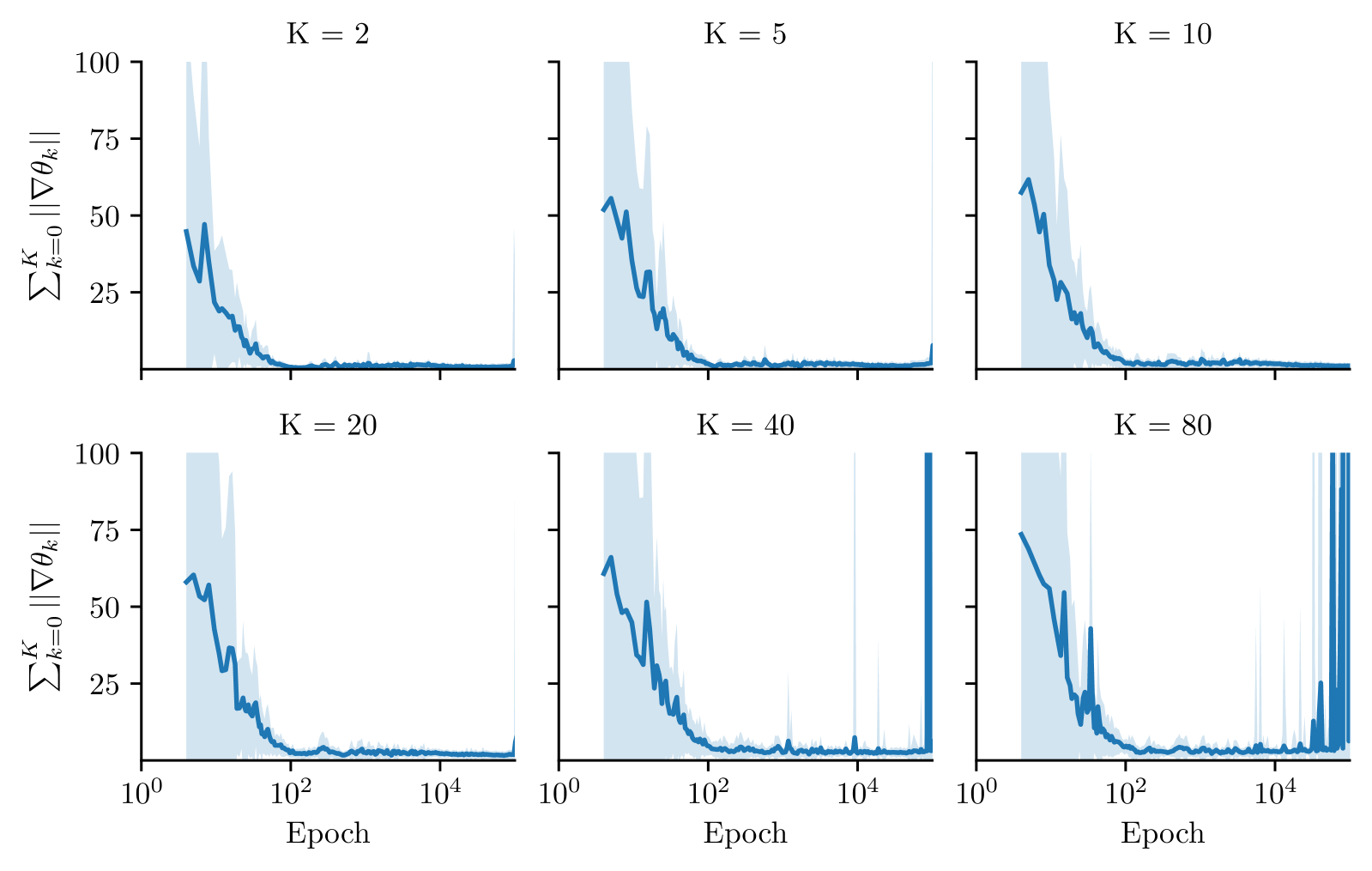
Figure 12: Additional results corresponding to Fig. 5, visualizing the gradient norm $\sum^{K}_{k=0}||\nabla\bm{\theta}_{k}||_{2}$ (y-axis) over the course of training epochs (x-axis). The color shading represents the $\pm$ standard deviation, computed from five independent repetitions and logarithmic binning of the epochs.

Additional results for non-zero weight decay are presented in Fig. 13.

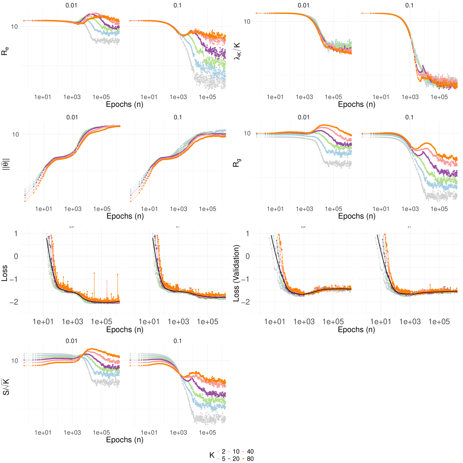
Figure 13: Additional results for non-zero weight decay $0.01$ and $0.1$

Appendix B Theoretical Results

Theorem 2 (Permutation Symmetries).

Assume each $\bm{\theta}_{k}\in\bm{\Lambda}$ satisfies $\bm{\theta}_{k,i}<\bm{\theta}_{k,i+1}$ for all its entries $i=1,...,D-1$, where $\bm{\theta}_{k,i}$ denotes the $i$-th component of $\bm{\theta}_{k}$. Define $S_{D}$ as the permutation group acting on $\mathbb{R}^{D}$ by permuting the components. For $\epsilon>0$ define

$$b_{\bm{\Lambda}}([0,1])_{\epsilon}:=\{\bm{\theta}\in\mathbb{R}^{D}\colon\exists t\in[0,1]\text{ s.t. }||b_{\bm{\Lambda}}(t)-\bm{\theta}||<\epsilon\}$$

as the “tunnel” of radius $\epsilon$ around the curve $b_{\bm{\Lambda}}$.

Then, there exists some $\epsilon>0$ such that for all $g\in S_{D}$ and all parameters $\bm{\theta}\in b_{\bm{\Lambda}}([0,1])_{\epsilon}$ it holds $g\bm{\theta}\notin b_{\bm{\Lambda}}([0,1])_{\epsilon}$.

Proof of Theorem 2.

By assumption, it holds $0<\min_{k=1,...,K,i=1,...,D-1}\bm{\theta}_{k,i+1}-\bm{\theta}_{k,i}$. Thus, there exists some $0<\epsilon<\min_{k=1,...,K,i=1,...,D-1}\bm{\theta}_{k,i+1}-\bm{\theta}_{k,i}/2$. It suffices to prove that any $\bm{\theta}\in b_{\bm{\Lambda}}([0,1])_{\epsilon}$ is ordered, i.e. $\bm{\theta}_{i}<\bm{\theta}_{i+1}$ for all $i=1,...,D-1$. Then, any permutation of $\bm{\theta}$ is not ordered and, therefore, not an element of $b_{\bm{\Lambda}}([0,1])_{\epsilon}$.

Let $\bm{\theta}\in b_{\bm{\Lambda}}([0,1])_{\epsilon}$. By definition, there exists some $t\in[0,1]$ such that $||b_{\bm{\Lambda}}(t)-\bm{\theta}||<\epsilon$. In particular,

$$\bm{\theta}_{i+1}-\bm{\theta}_{i}>b_{\bm{\Lambda}}(t)_{i+1}-b_{\bm{\Lambda}}(t)^{i}-2\epsilon.$$

Note that

$$\min_{i=1,...,D-1}b_{\bm{\Lambda}}(t)^{i+1}-b_{\bm{\Lambda}}(t)^{i}\geq\min_{k=1,...,K,i=1,...,D-1}\bm{\theta}_{k,i+1}-\bm{\theta}_{k,i}>2\epsilon>0$$

for all $t$ since $b_{\bm{\Lambda}}(t)$ is a finite linear combination of ordered vectors $\bm{\theta}_{k}$ with positive scalars (see (3)) and $\sum_{k=0}^{K}\binom{K}{k}(1-t)^{K-k}t^{k}=1$. Thus,

$$\bm{\theta}_{i+1}-\bm{\theta}_{i}>b_{\bm{\Lambda}}(t)_{i+1}-b_{\bm{\Lambda}}(t)_{i}-2\epsilon>0$$

which proves the claim. ∎

Appendix C Further Implementation Details

All implementation details, including the full set of hyperparameter configurations, model architecture specifications, and training procedures, are also provided in the supplementary code at https://github.com/doldd/Paths-and-Ambient-Spaces, with a dedicated README file to navigate through the experiments.

C.1 Sampling Algorithm

Algorithm 2 outlines the implementation of our tunnel-guided sampling routine, using Metropolis-Hastings as an example. The routine is, however, sampler-agnostic, and other sampling methods can also be applied. In our experiments, we primarily use the NUTS (Hoffman and Gelman,, 2014) sampler or the more efficient MCLMC (Robnik et al.,, 2023) sampler, with the implementation from the BlackJAX library.

Algorithm 2 Sampling

 define $\bm{\Xi}$-space from $\bm{\Lambda}^{\ast}$

 initialize Local coordinate system for RMF in $\bm{\Xi}$-space

 for #Chains & #Samples do

  Draw $t$ and $\bm{\xi}$ proposal

  Compute $\bm{\vartheta}=\bm{\Pi}g(t,\bm{\xi})$

  Compute likelihood $p(\mathcal{D}|\bm{\vartheta})$ and prior $p(t,\bm{\xi})$

  Adjust prior with $\log|\det({\partial g(t,\bm{\xi})}/{\partial t,\bm{\xi}})|$

  Accept/reject proposal according to MH

 end for

 return Samples from $p(t,\bm{\xi}|\mathcal{D})$

Appendix D Experimental Details

D.1 Datasets

D.1.1 Simulated Datasets

Our approach aligns with the approach by Wilson and Izmailov, (2020). Specifically, we randomly initialize neural network weights $\bm{\theta}_{\textrm{gen}}$, using the same architecture as in our later experiments, and generate the target labels as $y_{i}=f_{\bm{\theta}_{\textrm{gen}}}(x_{i})+\epsilon$, where $\epsilon\sim N(0,0.05)$. Both $x$ and the resulting target $y$ are one-dimensional for easy visualization. For the feature $x_{\textrm{train}}$ of the training dataset, we sample values uniformly distributed between $-2$ and $2$. We exclude values between $-0.6$ and $0.6$ to simulate in-between uncertainty, resulting in 70 training data points. Similarly, we generated 18 validation data points, which are in the same range as the training data, and 33 test data points in an extended range (cf. Fig. 14). This data generation process was repeated with newly initialized $\bm{\theta}_{\textrm{gen}}$ for each repetition of the synthetic dataset experiment. Fig. 14 shows all the generated data.

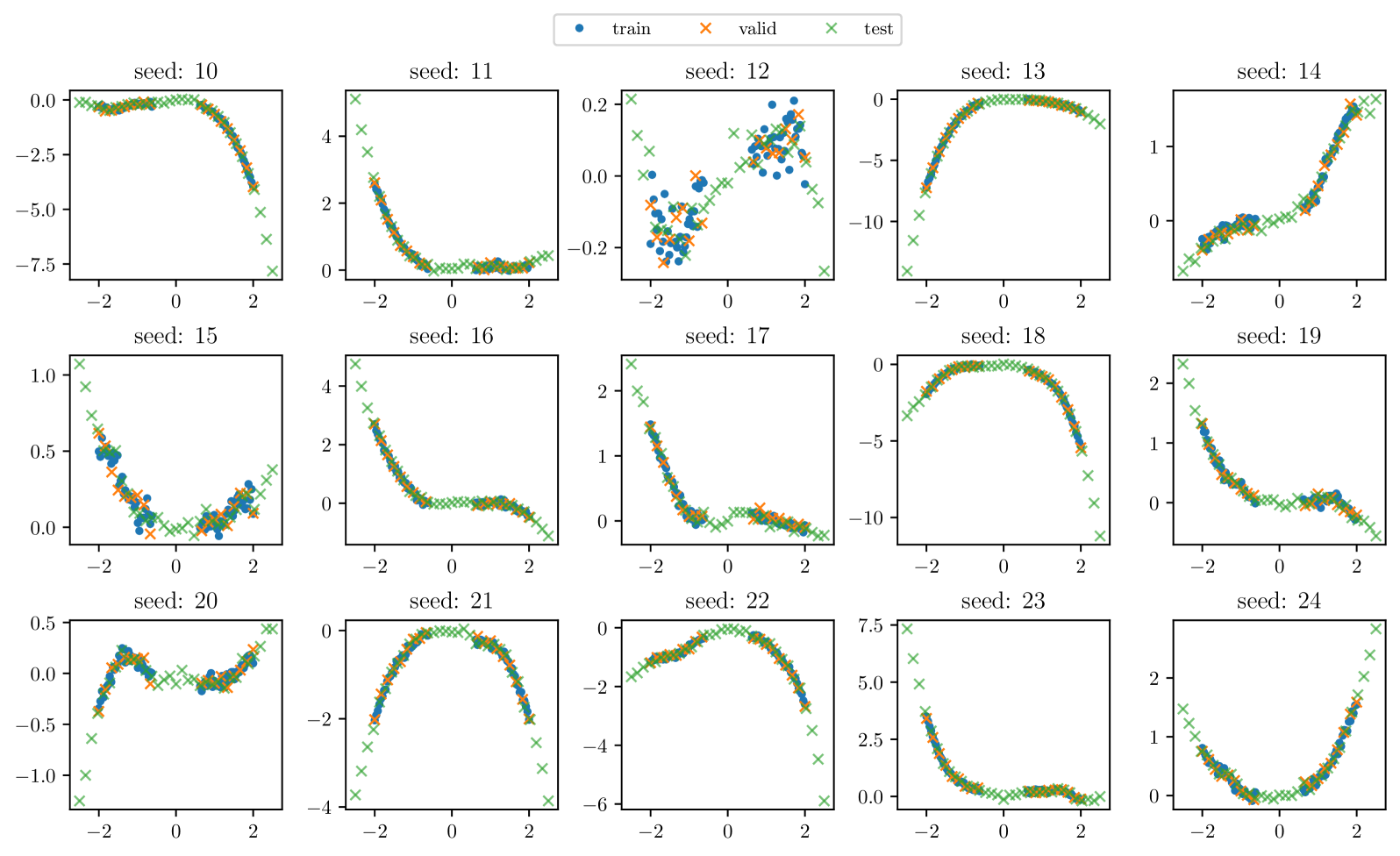
Figure 14: Synthetic generated regression data using a fully connected neural network with three hidden layers, each with 16 neurons and ReLU activation function.

D.1.2 Benchmark Datasets

Table 3 provides an overview of the benchmark data sets used in our experiments.

Table 3: Overview of the used benchmark datasets

Data set	Task	# Obs.	Feat.	Reference
airfoil	Regression	1503	5	Dua and Graff, (2017)
bikesharing	Regression	17379	13	Fanaee-T, (2013)
concrete	Regression	1030	8	Yeh, (1998)
energy	Regression	768	8	Tsanas and Xifara, (2012)
yacht	Regression	308	6	Ortigosa et al., (2007); Dua and Graff, (2017)
MNIST	Multi-Class.	60000	28x28	LeCun and Cortes, (2010)

We standardize the input data for the UCI regression tasks and also compute the LPPD (cf. Eq. 11) on the standardized data. For the MNIST dataset, we use 5-fold cross-validation on the train and validation set, where the 60,000 observations were split into one fold of $48\,000$ training data and $12\,000$ validation data, following their original order. The LPPD and RMSE for MCMC differ from the values reported in (Sommer et al.,, 2024) because they used a heteroscedastic approach, whereas we modeled the outcome distribution in a homoscedastic fashion. This choice was made because our focus is not on performing distributional regression, and heteroscedastic optimization comes with its own set of challenges.

D.2 Methods

Methods for Section 4.2 to Section 4.4

In experiments of Sections 4.2 and 4.4, our model is defined as a fully connected network with three hidden layers, each with 16 neurons. As an activation function, we use ReLU for the regression benchmarks in Section 4.4. In Section 4.2 and Section 4.3, we use both ReLU and ELU activations. The only difference in the model architecture for the simulated data and the UCI benchmark data is the inclusion of a feature expansion for the simulated data, where we extended $x$ to the feature vector $[x,x^{2},x^{3}]$.

For the Laplace Approximation (LA) method, we first train MAP solutions using the Adam optimizer with regularization for $10\,000$ epochs with a learning rate of $0.005$ and then use last-layer LA with a generalized Gauss-Newton Hessian approximation and a closed-form predictive approximation over five different initializations and splits (Daxberger et al.,, 2021).

For the deep ensembles (DE), we train 10 MAP solutions with different initializations using the training recipe described above for LA and average the predictions to obtain the performance results.

For the ModeCon method, we implement the approach described in Garipov et al., (2018), where we train two MAP-solutions $\bm{\theta}_{0},\bm{\theta}_{2}$ with different initializations as start- and endpoint of a Bézier curve and add a third randomly initialized model, $\bm{\theta}_{1}$, to obtain a quadratic Bézier curve with three control points, given by $\bm{\theta}_{0},\bm{\theta}_{1},\bm{\theta}_{2}$. In the subsequent curve training step, we keep the endpoints (MAP solutions) fixed and only apply loss-gradient-based updates to $\bm{\theta}_{1}$. We use early stopping by evaluating the path loss $L(\bm{\theta}_{0},\bm{\theta}_{1},\bm{\theta}_{2})$ at 50 uniformly spaced-out positions of $t$. After training the curve, we employ volume lifting as described in Section 2.5 and use the NUTS sampler to obtain posterior samples from the hyperplane. We use an isotropic Gaussian prior for the parameters of the hyperplane, consistent with Izmailov et al., (2020). Last, we define the orthogonal projection matrix $\bm{\Pi}$ using a principal component analysis of the centered control points $\bm{\theta}_{0},\bm{\theta}_{1},\bm{\theta}_{2}$, keeping the first two principal components to project the samples from the hyperplane to a neural network weight $\bm{\theta}\in\bm{\Theta}$.

For our Tunnel-2 method, we first initialize $\bm{\Lambda}=\{\bm{\theta}_{0},\bm{\theta}_{1},\bm{\theta}_{2}\}$ randomly and optimize these parameters jointly as described in Algorithm 1. We use the Adam optimizer and manually adjust the learning rate to stabilize the training loss. For the simulated data, we choose a learning rate of 0.001. For the UCI benchmark, the learning rate is set to 0.005. We run the entire training process for $100\,000$ epochs and the optimal parameters $\bm{\Lambda}^{\ast}$ are selected based on the validation performance of the curve. To compute the validation performance, we approximate the overall curve performance by averaging the log-likelihood evaluated at 1,000 evenly spaced grid points between zero and one for the curve parameter $t$.

For all consecutive sampling evaluations (tunnel vs. volume lifting, different temperatures), we use the same optimized path defined by $\bm{\Lambda}^{\ast}$, ensuring that no differences arise from variations in the optimized path. We use the MCLMC sampler from Robnik et al., (2023); Sommer et al., (2025) with 10 chains, 1000 warm-up samples, and 1000 collected samples. To reduce autocorrelation between samples and maintain comparability with NUTS, we increase the total number of samples by a factor of 100 but retain only every 100th sample. This simulates the leapfrog integration used in NUTS while maintaining a fixed computational budget.

In our Tunnel-K method, the setup is the same as in the Tunnel-2 configuration, with the difference that $\bm{\Lambda}$ consists of $K+1$ parameters instead of three, and a ($K-1$)-dimensional $\bm{\xi}$ during sampling.

Methods for Section 4.5

For the LA method, we train a MAP solution using the Adam optimizer with regularization for $5$ epochs with a batch size of $64$ and a learning rate of $0.001$. We use a last-layer LA with a generalized Gauss-Newton Hessian approximation and the Monte Carlo predictive approximation over five different initializations and splits (Daxberger et al.,, 2021).

For the Tunnel-$K$ method, we optimize the path using an Adam optimizer with a batch size of 480, over 50 epochs, and a learning rate of 0.005. We reduce the number of collected samples to 500, with 500 warm-up samples and 10 chains. Additionally, we add 10 extra steps per sample to simulate the behavior of the NUTS sampler within the MCLMC sampler. All other configurations remain the same as in the other experiments.

D.3 Performance Evaluation

To evaluate the performance of the subspace inference approaches on a set of previously unseen test data, we use the log pointwise predictive density (LPPD), which takes into account the posterior distribution (Gelman et al.,, 2014):

$$\text{LPPD}=\sum_{i=1}^{n_{obs}}\log\int p(y_{i}|\bm{\theta})p(\bm{\theta}|y_{i})d\bm{\theta}$$ (10)

In practical sampling-based inference, we evaluate the expectation using (vector-valued) draws from the posterior, $\bm{\theta}^{(u)},u=1,\dots,U$, and normalize the LPPD by the number of samples $n_{obs}$ to obtain a metric that is independent of the dataset size:

$$\widehat{\text{LPPD}}=\frac{1}{n_{obs}}\sum_{i=1}^{n_{obs}}\log\left(\frac{1}{U}\sum_{u=1}^{U}p(y_{i}|\bm{\theta}^{u})\right)$$ (11)

D.4 MCMC Sampling Evaluation

For the evaluation of the drawn posterior samples, we use the effective sample size (ESS; Vehtari et al.,, 2021) and R̂ (Gelman et al.,, 2014), where ESS is given by

$$\text{ESS}=\frac{U}{1+2\sum_{t=1}^{\infty}\rho_{t}}$$ (12)

and $\rho_{t}$ denotes the autocorrelation in a single MCMC chain at different lags $t$ (Vehtari et al.,, 2021; Stan Development Team,, 2024). The ESS of an MCMC chain quantifies the number of independent samples that an autocorrelated sequence effectively represents.

The potential scale reduction metric $\hat{R}$ is a convergence measure that compares within-chain variance $W$ and between-chain variance $B$ to assess chain convergence. When all chains have reached equilibrium, these variances will be equal, and $\hat{R}$ will be equal to $1$. However, if the chains have not converged to a common distribution, the statistic will exceed one (Stan Development Team,, 2024). Following the definition put forth by the Stan Development Team, (2024), on $M$ different chains, each chain containing $U$ samples $\theta^{(u)}_{m}$, the between-chain variance is defined as

$$B=\frac{U}{M-1}\,\sum_{m=1}^{M}(\bar{\theta}^{(\bullet)}_{m}-\bar{\theta}^{(\bullet)}_{\bullet})^{2}$$ (13)

where

$$\bar{\theta}_{m}^{(\bullet)}=\frac{1}{U}\sum_{u=1}^{U}\theta_{m}^{(u)}\quad\text{and}\quad\bar{\theta}^{(\bullet)}_{\bullet}=\frac{1}{M}\,\sum_{m=1}^{M}\bar{\theta}_{m}^{(\bullet)}.$$ (14)

The within-variance is given by

$$W=\frac{1}{M}\,\sum_{m=1}^{M}v_{m}^{2}\quad\text{with}\quad v_{m}^{2}=\frac{1}{U-1}\,\sum_{u=1}^{N}(\theta^{(u)}_{m}-\bar{\theta}^{(\bullet)}_{m})^{2}.$$ (15)

The variance estimator $\widehat{\mbox{var}}^{+}\!(\theta|y)$ is a mixture of the within-chain and cross-chain sample variances,

$$\widehat{\mbox{var}}^{+}\!(\theta|y)=\frac{U-1}{U}\,W\,+\,\frac{1}{U}\,B,\quad\text{with the final metric defined as}\quad\hat{R}\,=\,\sqrt{\frac{\widehat{\mbox{var}}^{+}\!(\theta|y)}{W}}.$$ (16)

D.5 Permutation Symmetries

As symmetric solutions would not differ in their functional outcomes, we inspect the functional outcome captured by the path along the curve in Fig. 15. The figure shows that our path does not collapse to one functional realization and the functional outcome differs along the curve. We also observe that a smooth transition occurs in the functional outcome as we travel along the curve.

Additionally, Fig. 15 shows that increasing the subspace dimension $K$ can improve the functional diversity captured by the path. Comparing the different path objectives, as discussed in Section 2.2, does not reveal significant differences and is included primarily for completeness.

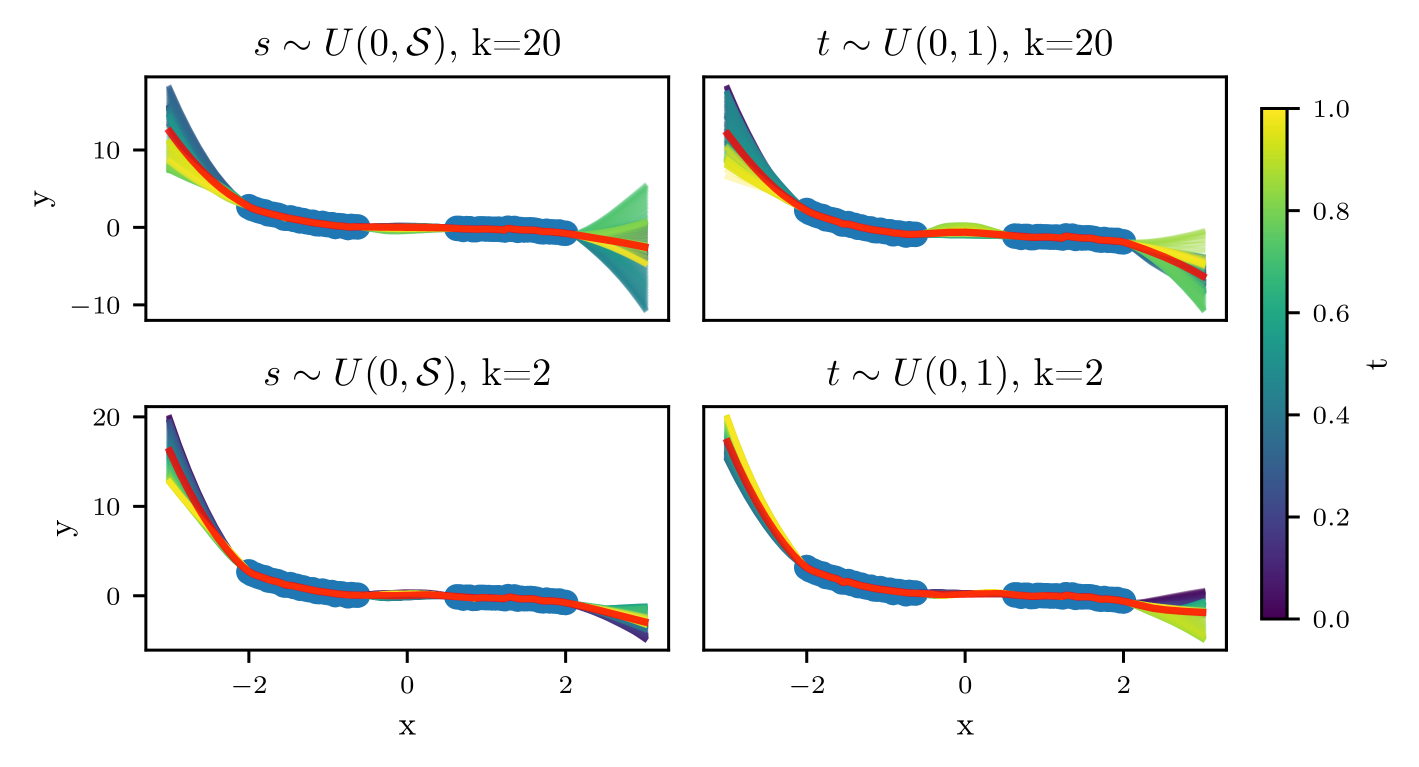
Figure 15: Investigating functional diversity on an exemplary synthetic dataset generated with ELU activation and seed $=16$. The columns compare two different path objectives: $t\sim U(0,1)$ and $s\sim U(0,\mathcal{S})$, while the rows compare subspace dimensions $K=2$ and $K=20$. The blue dots represent the training data, and the red line shows the averaged prediction along the entire curve. Each color corresponds to a single prediction at a specific $t$ or $s$ value. For simplicity, only the color legend for $t$ values is shown; the same color scheme applies to $s$.

To validate our Theorem 2, we modify the MLP network to implicitly incorporate bias parameters that are sorted in each layer to obtain permutation symmetry-free solutions according to Pourzanjani et al., (2017). Sorting is achieved by optimizing the unrestricted bias parameter $\bm{B^{\prime}}$ for every control point $\bm{\theta}_{k}$ and converting it into the original bias parameter $\bm{B}$ using

$$B_{i}=\sum_{j=0}^{i}\tilde{B}_{j},\quad\text{where}\quad\tilde{B}_{j}=\begin{cases}B^{\prime}_{0},&j=0\\ \ln(1+e^{B^{\prime}_{j}}),&j>0.\end{cases}$$ (17)

The results of this experiment are visualized in Fig. 16. We observe that the bias parameters are arranged in ascending order along the entire path defined by the Bézier curve. This indicates that adjusting only the control points results in a permutation-free path. This finding aligns with the theoretical framework established in Theorem 2.

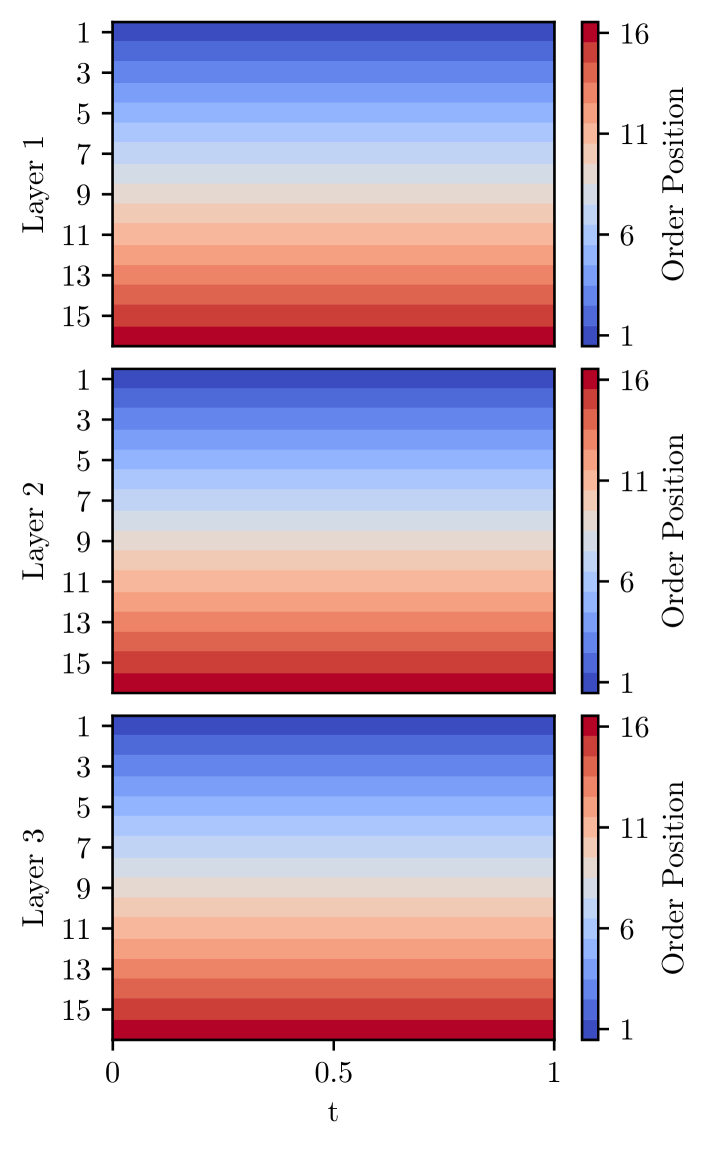
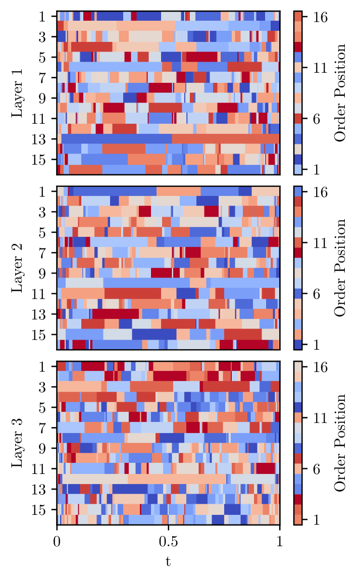
Figure 16: Left column: Bias ordering of a three-hidden-layer MLP with 16 neurons per layer. The Y-axis represents neurons in each layer (rows), color-coded according to their sorting index, while the X-axis represents the traversal along the path. Right column: Bias ordering in each layer when traversing the path without adjustment.

To further investigate how the adjustment of permutation symmetry influences performance, we compared both approaches — one with the adjustment of permutation symmetry by bias sorting and one without — in the regression data set used in Section 4.2. In Fig. 17, we observe that validation performance slightly decreases when enforcing a sorted bias parameter in each layer. This suggests that even without adjustment, the path does not contain harmful permutation symmetries. If such symmetries were present, eliminating all permutation-symmetric solutions would be expected to improve performance.

Figure 17: Averaged log-likelihood over the path on the validation data for increasing subspace dimension (x-axis) and different activation functions (columns). The different hues compare cases where the bias parameter was sorted (orange) versus left unchanged (blue).

D.6 Effects of Temperature

In addition to introducing a tunnel prior, incorporating a temperature parameter in the sampling process can help in better guiding the sampler through the tunnel. More specifically, by down-weighting the influence of the likelihood during sampling, we can facilitate better exploration of the tunnel, as the posterior distribution often becomes overly concentrated around the maximum likelihood estimate (MLE). This excessive concentration, in turn, can lead to overly confident uncertainty estimates by failing to explore the whole tunnel. As in other practical applications of temperature, where it is often found to yield better predictive accuracy if the likelihood is tempered with $\frac{1}{T}$ (Izmailov et al.,, 2020), we implement temperature scaling of the likelihood as: $p_{\text{temp}}(\bm{\theta}|\mathcal{D})\propto p(\mathcal{D}|\bm{\theta})^{1/T}p(\bm{\theta})$ or, expressed in log-space,

$$\log p_{\text{temp}}(\bm{\theta}|\mathcal{D})=\frac{1}{T}\log p(\mathcal{D}|\bm{\theta})+\log p(\bm{\theta})+\text{const}.$$ (18)

For $T=1$, the original posterior is recovered. As $T\rightarrow\infty$, $p_{\text{temp}}(\bm{\theta}|\mathcal{D})$ converges to the prior. The effect of $T$ on $\log p_{\text{temp}}(\bm{\theta}|\mathcal{D})$ is visualized in Fig. 18.

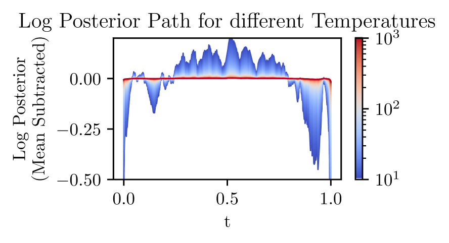
Figure 18: Unnormalized log posterior along the path for different temperature parameters using the Bézier curve trained on the yacht dataset. The averaged unnormalized log posterior along the curve was subtracted for each specific temperature value.

Appendix E Additional Numerical Results

E.1 Synthetic dataset

Fig. 19 provides additional results for the experiments discussed in Section 4.2. While in Section 4.2, the temperature parameter is selected based on the best LPPD performance on the validation data, Fig. 19 shows the LPPD performance across all temperature values. Notably, the optimal temperature depends on the subspace dimension $K$, with larger $K$ values requiring lower temperatures. This observation aligns with the motivation in Izmailov et al., (2020), which suggests adding temperature to account for the dimensional difference between the lower-dimensional subspace, where the prior is defined, and the high-dimensional weight space. As $K$ increases, these differences decrease, thus requiring smaller temperature parameters.

The comparison between the tunnel and volume-lifting approaches shows that the tunnel prior is more appropriate, as it performs better in the high-temperature range. Additionally, comparing networks with ReLU vs. ELU activations reveals only a minor difference in performance.

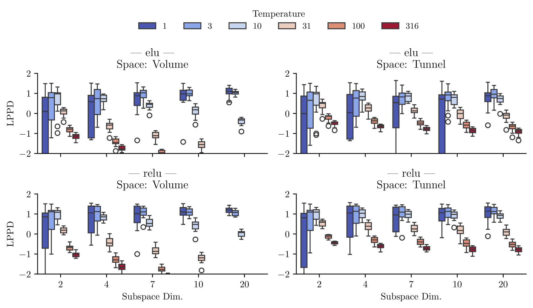
Figure 19: LPPD performance on the synthetic dataset using different temperature parameters. Each row compares a fully connected neural network with ELU activation versus ReLU activation and each column compares the volume versus tunnel-lifting approach.

E.2 Benchmark dataset

Fig. 20 shows different evaluated metrics for the benchmark dataset, depending on the temperature (x-axis), and compares the $K=2$ with the $K=20$ tunnel lifting (colors). We see the same behavior as in Fig. 19, i.e., $K=20$ requires lower temperatures.

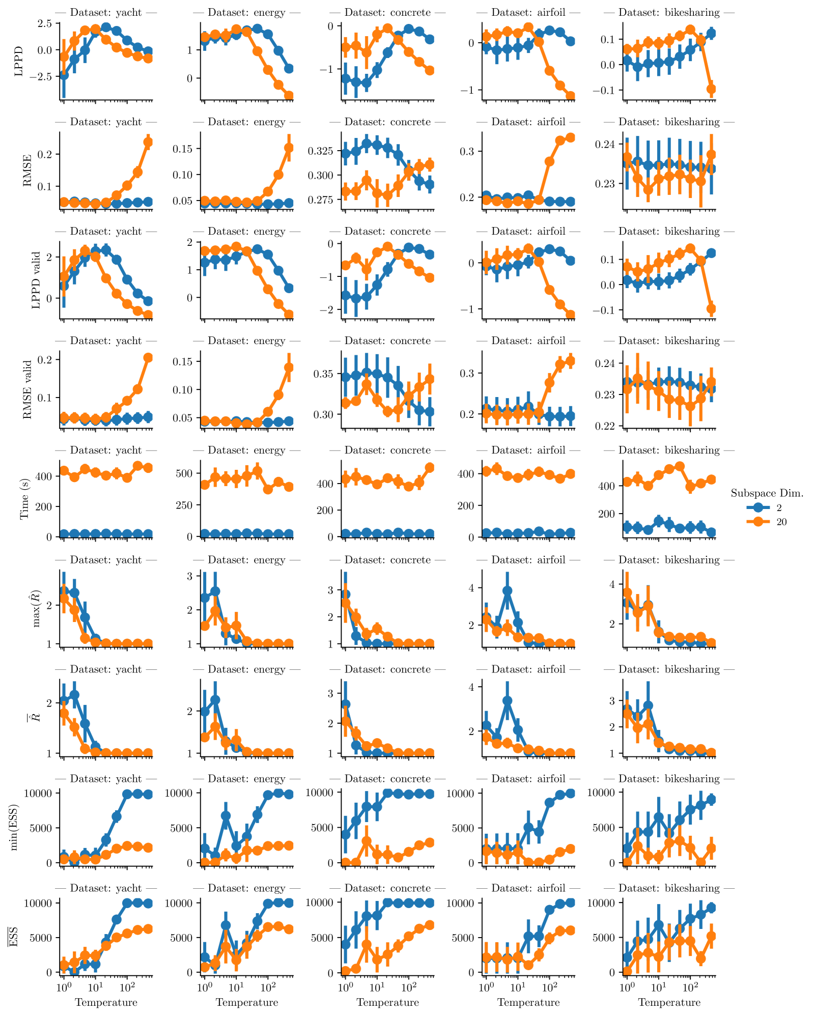
Figure 20: Different computed metrics (y-axis) versus temperature parameter (x-axis) for different datasets (columns). Colors represent the subspace dimension: $K=2$ (blue) and $K=20$ (orange). The error bars indicate the standard error across five repetitions. We compute the average and worst metrics for ESS and $\hat{R}$ across all model parameters. The metric “Time (s)” represents the wall clock time, measured in seconds, to sample 10 chains with 1000 samples per chain.

E.3 MNIST

Fig. 21 presents the same evaluation as in Fig. 8, but instead of using the best temperature selected based on the validation LPPD, the behavior across specific temperature parameters is visualized. We observe a trade-off between optimizing the temperature according to the LPPD metric and the accuracy, with accuracy favoring lower temperature values.

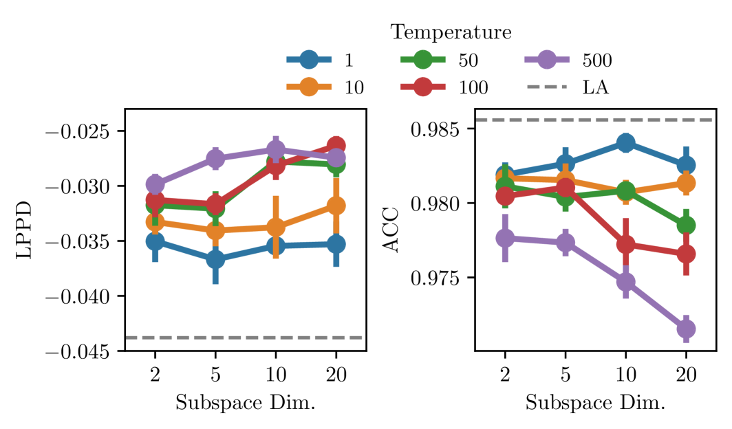
Figure 21: Performance on MNIST (with the standard error over five different folds) with different temperature parameters (color) and subspace dimensions $K$ (x-axis). The dashed line shows the results using Laplace Approximation (LA). The underlying path is optimized with $t\sim U(0,1)$ sampling.

Appendix F Computational Environment

The complexity of our dataset was intentionally kept manageable, allowing us to conduct experiments on consumer hardware, such as an NVIDIA 3080Ti GPU with 11GB of VRAM. While the 11GB of VRAM was not essential, it did improve runtime by enabling parallel execution of multiple chains during the sampling process. Only for the MNIST dataset, where we performed full-batch evaluations during sampling, we resorted to a Titan RTX GPU with 24GB of VRAM to accommodate the increased memory requirements.

From an implementation perspective, our experiments were conducted using the JAX library (Bradbury et al.,, 2018), in combination with Flax to specify the model architecture. The same model description was used to define our sampling model within the NumPyro framework, and sampling was performed using BlackJAX, which specified the sampler. For reproducibility, all runs were tracked using a local instance of “Weights & Biases”, which was also used to collect the data needed to generate the figures.

References

- Adilova et al., (2024) Adilova, L., Andriushchenko, M., Kamp, M., Fischer, A., and Jaggi, M. (2024). Layer-wise linear mode connectivity. In The Twelfth International Conference on Learning Representations.
- Ainsworth et al., (2023) Ainsworth, S., Hayase, J., and Srinivasa, S. (2023). Git re-basin: Merging models modulo permutation symmetries. In The Eleventh International Conference on Learning Representations.
- Azizian et al., (2024) Azizian, W., Iutzeler, F., Malick, J., and Mertikopoulos, P. (2024). What is the long-run distribution of stochastic gradient descent? a large deviations analysis.
- Benton et al., (2021) Benton, G., Maddox, W., Lotfi, S., and Wilson, A. G. G. (2021). Loss surface simplexes for mode connecting volumes and fast ensembling. In International Conference on Machine Learning, pages 769–779. PMLR.
- Benzing et al., (2022) Benzing, F., Schug, S., Meier, R., Von Oswald, J., Akram, Y., Zucchet, N., Aitchison, L., and Steger, A. (2022). Random initialisations performing above chance and how to find them. In OPT 2022: Optimization for Machine Learning (NeurIPS 2022 Workshop).
- Bradbury et al., (2018) Bradbury, J., Frostig, R., Hawkins, P., Johnson, M. J., Leary, C., Maclaurin, D., Necula, G., Paszke, A., VanderPlas, J., Wanderman-Milne, S., and Zhang, Q. (2018). JAX: composable transformations of Python+NumPy programs.
- Daxberger et al., (2021) Daxberger, E., Kristiadi, A., Immer, A., Eschenhagen, R., Bauer, M., and Hennig, P. (2021). Laplace redux-effortless bayesian deep learning. Advances in Neural Information Processing Systems, 34:20089–20103.
- De Gennes, (1979) De Gennes, P. (1979). Scaling Concepts in Polymer Physics. Cornell University Press.
- Dold et al., (2024) Dold, D., Rügamer, D., Sick, B., and Dürr, O. (2024). Bayesian semi-structured subspace inference. In International Conference on Artificial Intelligence and Statistics, pages 1819–1827. PMLR.
- Draxler et al., (2018) Draxler, F., Veschgini, K., Salmhofer, M., and Hamprecht, F. (2018). Essentially no barriers in neural network energy landscape. In Dy, J. and Krause, A., editors, Proceedings of the 35th International Conference on Machine Learning, volume 80 of Proceedings of Machine Learning Research, pages 1309–1318. PMLR.
- Dua and Graff, (2017) Dua, D. and Graff, C. (2017). UCI machine learning repository.
- Entezari et al., (2022) Entezari, R., Sedghi, H., Saukh, O., and Neyshabur, B. (2022). The role of permutation invariance in linear mode connectivity of neural networks. In International Conference on Learning Representations.
- Fanaee-T, (2013) Fanaee-T, H. (2013). Bike Sharing Dataset. UCI Machine Learning Repository.
- Fort and Jastrzebski, (2019) Fort, S. and Jastrzebski, S. (2019). Large scale structure of neural network loss landscapes. Advances in Neural Information Processing Systems, 32.
- Frankle et al., (2020) Frankle, J., Dziugaite, G. K., Roy, D., and Carbin, M. (2020). Linear mode connectivity and the lottery ticket hypothesis. In International Conference on Machine Learning, pages 3259–3269. PMLR.
- Frenet, (1852) Frenet, F. (1852). Sur les courbes à double courbure. Journal de mathématiques pures et appliquées, 17:437–447.
- Garipov et al., (2018) Garipov, T., Izmailov, P., Podoprikhin, D., Vetrov, D. P., and Wilson, A. G. (2018). Loss surfaces, mode connectivity, and fast ensembling of dnns. Advances in neural information processing systems, 31.
- Gelman et al., (2014) Gelman, A., Hwang, J., and Vehtari, A. (2014). Understanding predictive information criteria for bayesian models. Statistics and computing, 24:997–1016.
- Gotmare et al., (2018) Gotmare, A., Keskar, N. S., Xiong, C., and Socher, R. (2018). Using mode connectivity for loss landscape analysis. arXiv preprint arXiv:1806.06977.
- Hoffman and Gelman, (2014) Hoffman, M. D. and Gelman, A. (2014). The no-u-turn sampler: Adaptively setting path lengths in hamiltonian monte carlo. Journal of Machine Learning Research, 15(47):1593–1623.
- Izmailov et al., (2020) Izmailov, P., Maddox, W. J., Kirichenko, P., Garipov, T., Vetrov, D., and Wilson, A. G. (2020). Subspace inference for bayesian deep learning. In Uncertainty in Artificial Intelligence, pages 1169–1179. PMLR.
- Lakshminarayanan et al., (2017) Lakshminarayanan, B., Pritzel, A., and Blundell, C. (2017). Simple and scalable predictive uncertainty estimation using deep ensembles. In Advances in Neural Information Processing Systems, volume 30. Curran Associates, Inc.
- LeCun and Cortes, (2010) LeCun, Y. and Cortes, C. (2010). MNIST handwritten digit database.
- Lin et al., (2024) Lin, Z., Li, P., and Wu, L. (2024). Exploring neural network landscapes: Star-shaped and geodesic connectivity. arXiv preprint arXiv:2404.06391.
- Lubana et al., (2023) Lubana, E. S., Bigelow, E. J., Dick, R. P., Krueger, D., and Tanaka, H. (2023). Mechanistic mode connectivity. In International Conference on Machine Learning, pages 22965–23004. PMLR.
- Ortigosa et al., (2007) Ortigosa, I., Lopez, R., and Garcia, J. (2007). A neural networks approach to residuary resistance of sailing yachts prediction. In Proceedings of the International Conference on Marine Engineering (MARINE), volume 2007, page 250.
- Pittorino et al., (2022) Pittorino, F., Ferraro, A., Perugini, G., Feinauer, C., Baldassi, C., and Zecchina, R. (2022). Deep networks on toroids: removing symmetries reveals the structure of flat regions in the landscape geometry. In International Conference on Machine Learning, pages 17759–17781. PMLR.
- Pourzanjani et al., (2017) Pourzanjani, A. A., Jiang, R. M., and Petzold, L. R. (2017). Improving the Identifiability of Neural Networks for Bayesian Inference. In Second Workshop on Bayesian Deep Learning.
- Robnik et al., (2023) Robnik, J., Luca, G. B. D., Silverstein, E., and Seljak, U. (2023). Microcanonical hamiltonian monte carlo. Journal of Machine Learning Research, 24(311):1–34.
- Serret, (1851) Serret, J.-A. (1851). Sur quelques formules relatives à la théorie des courbes à double courbure. Journal de mathématiques pures et appliquées, 16:193–207.
- Sommer et al., (2025) Sommer, E., Robnik, J., Nozadze, G., Seljak, U., and Rügamer, D. (2025). Microcanonical langevin ensembles: Advancing the sampling of bayesian neural networks. In The Thirteenth International Conference on Learning Representations.
- Sommer et al., (2024) Sommer, E., Wimmer, L., Papamarkou, T., Bothmann, L., Bischl, B., and Rügamer, D. (2024). Connecting the dots: Is mode-connectedness the key to feasible sample-based inference in Bayesian neural networks? In Proceedings of the 41st International Conference on Machine Learning, volume 235 of Proceedings of Machine Learning Research, pages 45988–46018. PMLR.
- Sonthalia et al., (2024) Sonthalia, A., Rubinstein, A., Abbasnejad, E., and Oh, S. J. (2024). Do deep neural network solutions form a star domain? arXiv preprint arXiv:2403.07968.
- Stan Development Team, (2024) Stan Development Team (2024). Stan modeling language users guide and reference manual.
- Tan et al., (2023) Tan, C., Long, T., Zhao, S., and Laine, R. (2023). Geodesic mode connectivity. arXiv preprint arXiv:2308.12666.
- Tatro et al., (2020) Tatro, N., Chen, P.-Y., Das, P., Melnyk, I., Sattigeri, P., and Lai, R. (2020). Optimizing mode connectivity via neuron alignment. Advances in Neural Information Processing Systems, 33:15300–15311.
- Tsanas and Xifara, (2012) Tsanas, A. and Xifara, A. (2012). Accurate quantitative estimation of energy performance of residential buildings using statistical machine learning tools. Energy and Buildings, 49:560–567.
- Vehtari et al., (2021) Vehtari, A., Gelman, A., Simpson, D., Carpenter, B., and Bürkner, P.-C. (2021). Rank-normalization, folding, and localization: An improved R-hat for assessing convergence of MCMC (with discussion). Bayesian analysis, 16(2):667–718.
- Wang et al., (2008) Wang, W., Jüttler, B., Zheng, D., and Liu, Y. (2008). Computation of rotation minimizing frames. ACM Transactions on Graphics (TOG), 27(1):1–18.
- Wilson and Izmailov, (2020) Wilson, A. G. and Izmailov, P. (2020). Bayesian deep learning and a probabilistic perspective of generalization. Advances in neural information processing systems, 33:4697–4708.
- Wortsman et al., (2022) Wortsman, M., Ilharco, G., Gadre, S. Y., Roelofs, R., Gontijo-Lopes, R., Morcos, A. S., Namkoong, H., Farhadi, A., Carmon, Y., Kornblith, S., et al. (2022). Model soups: averaging weights of multiple fine-tuned models improves accuracy without increasing inference time. In International conference on machine learning, pages 23965–23998. PMLR.
- Yeh, (1998) Yeh, I.-C. (1998). Modeling of strength of high-performance concrete using artificial neural networks. Cement and Concrete research, 28(12):1797–1808.
- Zhao et al., (2023) Zhao, B., Dehmamy, N., Walters, R., and Yu, R. (2023). Understanding mode connectivity via parameter space symmetry. In UniReps: the First Workshop on Unifying Representations in Neural Models.
- Zhao et al., (2020) Zhao, P., Chen, P.-Y., Das, P., Ramamurthy, K. N., and Lin, X. (2020). Bridging mode connectivity in loss landscapes and adversarial robustness. In International Conference on Learning Representations.