Constraints on inflationary decoherence from attractor model
Abstract
The quantum-to-classical transition of inflationary perturbations remains a fundamental challenge in cosmology, and quantum decoherence is one of the proposed solutions to this issue. By treating primordial quantum perturbations as an open quantum system interacting with environmental degrees of freedom during inflation, decoherence can be described by the Lindblad master equation. Lindblad equation modifies the dynamical evolution of the primordial quantum perturbations and affects the power spectrum of the curvature perturbations, resulting in changes in the primordial power spectrum. In this paper, we examine the decoherence process of a polynomial attractor model that includes an ultra-slow-roll plateau. We compare our findings with previous results from slow-roll analyses. We numerically compute the corrections to the power spectrum due to decoherence. The results show significant modifications only on large scales, with a peak appearing at the minimum of the power spectrum. Using CMB constraints on the spectral index and tensor-to-scalar ratio, and requiring complete decoherence for relevant scales by the end of inflation, we constrain the interaction parameter: .
I Introduction
The inflationary theory is one of the most successful theories in cosmology today. It assumes that the universe experienced a rapid expansion in its very early stages, which naturally addresses the horizon and flatness problems of the universe [1, 2, 3, 4, 5]. The primordial quantum fluctuations during the inflationary epoch can provide the primordial density perturbations that lead to the formation of large-scale structures (LSS) in the universe and anisotropies in the Cosmic Microwave Background (CMB) radiation [6, 7, 8, 9, 10, 11], which is supported by observations [12].
However, inflationary theory faces several unresolved challenges, with one of the most important being the quantum-to-classical transition problem [13, 14, 15, 16, 17, 18, 19, 20, 21, 22, 23, 24, 25, 26, 27, 28, 29, 30, 31, 32, 33, 34, 35, 36, 37]. The observational quantities in modern cosmology, including the temperature anisotropies of the CMB and the statistical properties of the LSS, demonstrate classical behavior. The question is how the primordial quantum fluctuations that seeded these structures made the transition to classical ones. A central issue arises from modeling primordial quantum perturbations as isolated systems. In reality, these perturbations interact with environmental degrees of freedom, leading to decoherence [38, 39, 40] that effectively converts quantum fluctuations into classical stochastic density inhomogeneities.
The dynamics of an open quantum system are described by the Lindblad master equation [41], which describes the time evolution of a quantum system interacting with an external environment. Under the environmental interactions, decoherence suppresses the off-diagonal elements of the system’s density matrix, driving it to a diagonal state [42, 43, 44]. This equation leads to a correction to the outcomes of the primordial perturbations, thereby affecting their power spectrum. In this paper, we consider the effect of decoherence and numerically compute the modified power spectrum of a inflationary model with an ultra-slow-roll stage. Moreover, we constrain the interaction parameter from the CMB observations.
The process of decoherence takes time and is considered complete when the off-diagonal elements of the quantum system’s density matrix become negligible. The decoherence time depends on the strength of the interaction between the system and its environment: stronger coupling leads to shorter timescales. On cosmological scales, the primordial quantum perturbations undergo complete decoherence by the end of inflation, thereby transitioning to a classical state. In this paper, we require that decoherence occurs sufficiently at the scale of interest, which imposes a lower bound constraint on the interaction parameter.
This paper is organized as follows. In Sec. II, we present the Lindblad equation that the quantum perturbations satisfy during inflation, along with its exact solution under the assumption of linear interactions. In Sec. III, we provide the parameters of our model and present the results of numerical calculations regarding the impact of decoherence, as well as constraints on the interaction strength. We summarize this paper in Sec. IV.
II Lindblad equation and the modified power spectrum
The inflationary curvature perturbation is described by the gauge-invariant Mukhanov-Sasaki scalar variable [6]. The free Hamiltonian of the perturbation in Fourier space is
| (1) |
where is the Mukhanov-sasaki variable in Fourier space and is its conjugate momentum, which obeys . A prime denotes a derivative with respect to conformal time . The frequency of mode is given by
| (2) |
where is the first slow-roll parameter, , with representing the Hubble parameter and a dot indicating differentiation with respect to time. The Hamiltonian (1) describes a isolated system. However, the primordial perturbations could interact with other degrees of freedom in the early universe, making it more realistic to consider the perturbations as an open quantum system [32, 35].
For an open quantum system that interacts with the environment, we can describe the total system in the Hilbert space , where the total Hamiltonian is
| (3) |
where is the Hamiltonian of the system, which acts in , and is the Hamiltonian of the environment, which acts in , is the interaction Hamiltonian and is the coupling constant. Suppose that the system and the environment only couple through local interactions, then the interaction Hamiltonian can be written as
| (4) |
where acts as a local operator within the system’s subsystem, while represents a local operator associated with the environmental component. The symbol represents the conformal spatial coordinate. According to the reasons mentioned in [32, 35], we can consider to have the form
| (5) |
where is a constant. By tracing out the environmental degrees of freedom from the total density matrix , we can derive the reduced density matrix for the system
| (6) |
Using the Born and Markov approximations, we can derive the equation of motion of , i.e. the Lindblad equation [41, 42, 32]
| (7) |
where with being the conformal auto-correlation time of , and is the same-time correlation function of , given by . We assume that the time-dependent parameter depends on the scale factor as a power law [32]
| (8) |
where denotes a reference time when the pivot scale crosses the Hubble radius, and is a free parameter. Assuming the environment to be isotropic and statistically homogeneous, can be defined as a top hat function [32]
| (9) |
where is a characteristic physical correlation length and
| (10) |
Expanding Eq. (9) in Fourier space, we can obtain
| (11) |
Considering the case where the environment consists of a heavy scalar field with mass , and the interaction Hamiltonian is
| (12) |
where the parameter is defined as a constant mass scale and . In this case, the parameters can be represented as [32]
| (13) | ||||
| (14) | ||||
| (15) |
where denotes the double factorial and
| (16) |
In order to solve the Lindblad equation (7), we decompose and into their real and imaginary parts
| (17) |
For a real operator , we have , which implies and . These relations show that not all operators are independent degrees of freedom, we can calculate the variables and in . Under the condition of linear interaction, the free Hamiltonian (1) can be written as
| (18) |
where . For linear interaction , the density matrix can be decomposed as
| (19) |
then we can obtain the Lindblad equation in the Fourier space for linear interaction [32]
| (20) |
Note that Eq. (20) is valid only for linear interaction. We can define a combined interaction parameter as follows
| (21) |
which combines all the parameters of interaction and possesses the dimension of comoving wavenumber.
Then we define the eigenvectors of the operator , which satisfy equation . By applying the bra and the ket to the Lindblad equation Eq. (20), the Lindblad equation can be solved exactly, the solution is given by [32]
| (22) |
where , and are defined by
| (23) | ||||
| (24) | ||||
| (25) |
where is the solution of the Mukhanov-Sasaki equation. Using Eq. (II) and the relation with , we can obtain the two-point correlation function
| (26) |
where is the standard two-point correlation and is the correction from the interaction with the environment. The modified power spectrum is
| (27) |
where we take . On the other hand, for linear interaction, the tensor power spectrum remains unchanged by the corrections in the Lindblad equation [35]. Therefore, we can utilize the spectral index and the tensor-to-scalar ratio to constrain for linear interaction.
The interaction with the environment tends to suppress the off-diagonal elements of the density matrix when expressed in the basis of the eigenstates of the interaction operator [42, 32]. From the exact solution of the density matrix Eq. (II), we can study decoherence during inflation. The decoherence parameter defined in [32] represents the reduction in the off-diagonal elements of the density matrix due to environmental interactions, and is defined as follows
| (28) |
It is obvious that is related to . When , decoherence is expected to be complete. We determine that by the end of inflation, the decoherence of the scales of interest should be finished, which in turn constrains .
In the study referenced as [32], the researchers took into account the constant and the constant Hubble parameter . In this paper, we will compute the results for a concrete model with an ultra-slow-roll stage. We compare the results of our model’s numerical computations with the analytical results reported in [32]. Then, we constraint using the polynomial attractor model.
III Models and numerical results
We choose the modified polynomial attractor model in [45]
| (29) |
where , the parameters of the model are given by Table. 1.
From Eq. (8) and (15), we can see that for linear interaction,
| (30) |
From Eq. (11) and (13), we have
| (31) |
where
| (32) |
Combine Eq. (24), (30)and (31), we have
| (33) |
The remaining sector of Eq. (24) can be written as
| (34) |
We take so that in Eq. (15) vanishes. In order to compare with [32], we take and . The top hat function in Eq. (III) can be written as
| (35) |
Then we can calculate the modified power spectrum numerically.
| Models | |||||||||
|---|---|---|---|---|---|---|---|---|---|
| A1 | 8.33 | 1.1007 | -1.07 | 3.2 | 3.75 | 63.2 | 0.9658 | 0.025 |
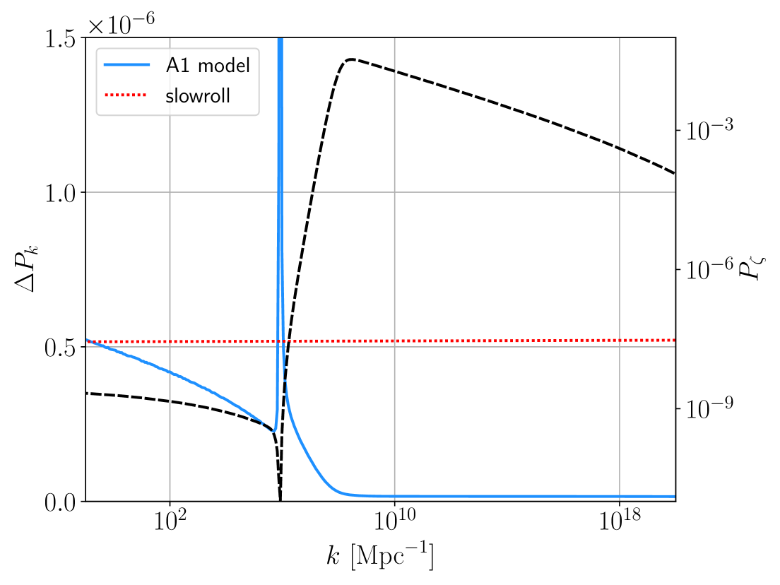
We calculate the modified term of the attractor model A1. The results of the modified power spectrum and are shown in Fig. 1. From Fig. 1, we see that at the pivot scale , both the slow-roll model and ultra-slow-roll model have the same value of . However, as the Hubble parameter gradually decreases, also decreases. We also find that at the minimum of the power spectrum, has a peak in the order of , but the correction near the peak is negligible (). This means that the correction due to decoherence almost does not change the abundance of primordial black holes and the scalar induced gravitational waves.
From Fig. 1, we find that the correction at pivot scale is more significant, which means that we can restrict using the spectral tilt and the tensor-to-scalar ratio at pivot scale. The analytical results for and in the case of linear interaction are [32]
| (36) |
and
| (37) |
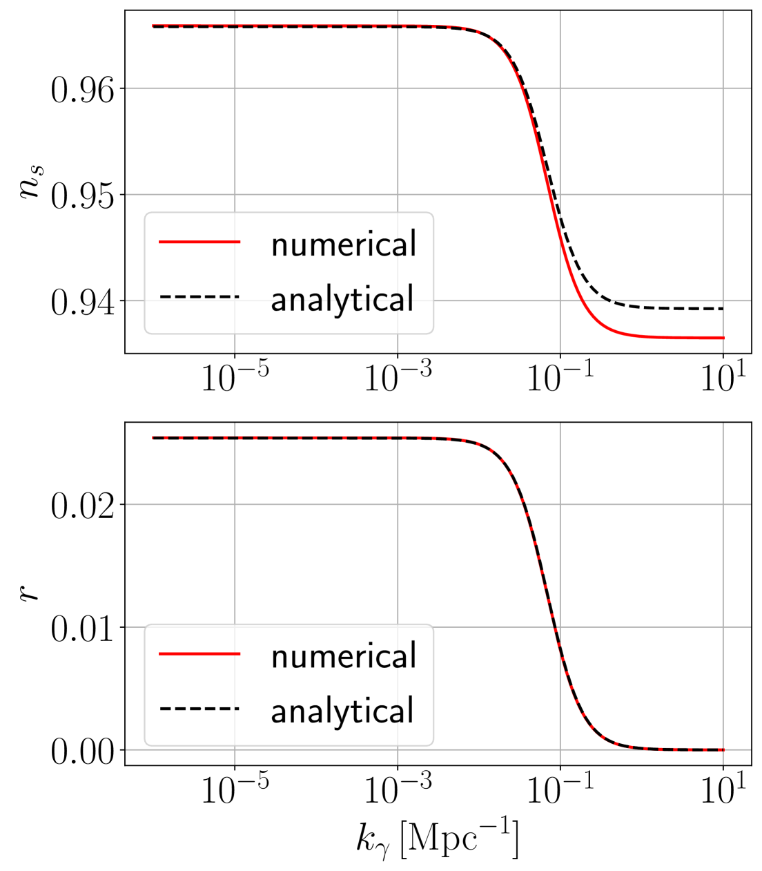
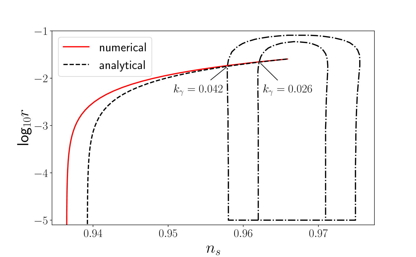
We perform numerical computations to determine the relationships between , and . The results are shown in Fig. 2. We can see that when , the results begin to change significantly, when , the changes in the results are minimal. The tensor-to-scalar ratios are well-aligned, whereas the spectral tilts deviate at large . We plot the results in the plane to restrict the upper bound of , the results are shown in Fig. 3. Starting from the initial point, as grows, both and diminish. When and , the results are within the and confidence intervals of the observation, respectively. This is the upper bound of given by model A1.
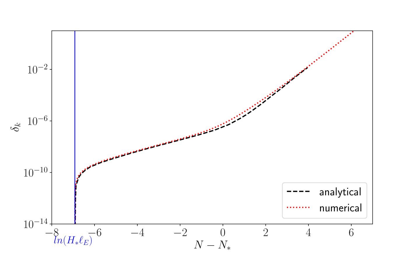
We then calculate the decoherence parameter at pivot scale and compare with the result in [32]. The results are shown in Fig. 4. Since model A1 is in the slow-roll stage at the pivot scale, the analytical and numerical results are almost the same. After , increase exponentially. We require that for the scales and , decoherence is complete. For model A1, this imposes a constraint on such that must be much greater than . This is a rather relaxed constraint.
IV Conclusion
In this paper, we examine the effects of decoherence on the power spectrum of a specific inflationary model that incorporates an ultra-slow-roll phase. Decoherence arises from the interaction of a quantum system with its environment and is described by the Lindblad equation. Based on the solutions to the Lindblad equation for linear interactions provided by J. Martin et al. [32], we numerically computed the corrections to the power spectrum of a polynomial attractor model due to quantum decoherence and constrained the interaction parameters using observations. We found that decoherence significantly alters the power spectrum only on large scales, and it is consistent with previous work at the pivot scales. As the scale decreases, the corrections to the power spectrum due to decoherence also diminish, and at the trough of the power spectrum, the corrections will result in a peak. We also calculated the relationship between the spectral index and the tensor-to-scalar ratio at the CMB with , and using the observational data from Planck 2018, we determined an upper limit for of Mpc-1. We calculate the decoherence parameter , which is used to characterize the degree of completion of decoherence; decoherence is considered to be complete when . We computed the evolution of over time at the pivot scale, and the results are roughly consistent with the analysis of the slow-roll regime. We require that decoherence be completed at the peak scale of the power spectrum by the end of inflation, which will provide a lower limit for the interaction parameter . Our model suggests a lower limit of . Since exact solutions are only provided for linear interactions, the aforementioned numerical calculations must satisfy the conditions of linear interaction.
References
- Guth [1981] A. H. Guth, Phys. Rev. D 23, 347 (1981).
- Linde [1982] A. D. Linde, Phys. Lett. B 108, 389 (1982).
- Albrecht and Steinhardt [1982] A. Albrecht and P. J. Steinhardt, Phys. Rev. Lett. 48, 1220 (1982).
- Starobinsky [1980] A. A. Starobinsky, Phys. Lett. B 91, 99 (1980).
- Sato [1981] K. Sato, Mon. Not. Roy. Astron. Soc. 195, 467 (1981).
- Mukhanov and Chibisov [1981] V. F. Mukhanov and G. V. Chibisov, JETP Lett. 33, 532 (1981).
- Guth and Pi [1982] A. H. Guth and S. Y. Pi, Phys. Rev. Lett. 49, 1110 (1982).
- Hawking [1982] S. W. Hawking, Phys. Lett. B 115, 295 (1982).
- Bardeen et al. [1983] J. M. Bardeen, P. J. Steinhardt, and M. S. Turner, Phys. Rev. D 28, 679 (1983).
- Mukhanov [1985] V. F. Mukhanov, JETP Lett. 41, 493 (1985).
- Sasaki [1986] M. Sasaki, Prog. Theor. Phys. 76, 1036 (1986).
- Akrami et al. [2020] Y. Akrami et al. (Planck), Astron. Astrophys. 641, A10 (2020), arXiv:1807.06211 [astro-ph.CO] .
- Starobinsky [1986] A. A. Starobinsky, Lect. Notes Phys. 246, 107 (1986).
- Brandenberger et al. [1990] R. H. Brandenberger, R. Laflamme, and M. Mijic, Mod. Phys. Lett. A 5, 2311 (1990).
- Polarski and Starobinsky [1996] D. Polarski and A. A. Starobinsky, Class. Quant. Grav. 13, 377 (1996), arXiv:gr-qc/9504030 .
- Calzetta and Hu [1995] E. Calzetta and B. L. Hu, Phys. Rev. D 52, 6770 (1995), arXiv:gr-qc/9505046 .
- Lesgourgues et al. [1997] J. Lesgourgues, D. Polarski, and A. A. Starobinsky, Nucl. Phys. B 497, 479 (1997), arXiv:gr-qc/9611019 .
- Burgess and Michaud [1997] C. P. Burgess and D. Michaud, Annals Phys. 256, 1 (1997), arXiv:hep-ph/9606295 .
- Kiefer et al. [1998] C. Kiefer, D. Polarski, and A. A. Starobinsky, Int. J. Mod. Phys. D 7, 455 (1998), arXiv:gr-qc/9802003 .
- Perez et al. [2006] A. Perez, H. Sahlmann, and D. Sudarsky, Class. Quant. Grav. 23, 2317 (2006), arXiv:gr-qc/0508100 .
- Lombardo and Lopez Nacir [2005] F. C. Lombardo and D. Lopez Nacir, Phys. Rev. D 72, 063506 (2005), arXiv:gr-qc/0506051 .
- Campo and Parentani [2006] D. Campo and R. Parentani, Phys. Rev. D 74, 025001 (2006), arXiv:astro-ph/0505376 .
- Ellis [2006] G. F. R. Ellis, “Issues in the philosophy of cosmology,” in Philosophy of physics, edited by J. Butterfield and J. Earman (2006) pp. 1183–1285, arXiv:astro-ph/0602280 .
- Martineau [2007] P. Martineau, Class. Quant. Grav. 24, 5817 (2007), arXiv:astro-ph/0601134 .
- Sharman and Moore [2007] J. W. Sharman and G. D. Moore, JCAP 11, 020 (2007), arXiv:0708.3353 [gr-qc] .
- Kiefer and Polarski [2009] C. Kiefer and D. Polarski, Adv. Sci. Lett. 2, 164 (2009), arXiv:0810.0087 [astro-ph] .
- Valentini [2010] A. Valentini, Phys. Rev. D 82, 063513 (2010), arXiv:0805.0163 [hep-th] .
- Sudarsky [2011] D. Sudarsky, Int. J. Mod. Phys. D 20, 509 (2011), arXiv:0906.0315 [gr-qc] .
- Asselmeyer-Maluga and Król [2013] T. Asselmeyer-Maluga and J. Król, Mod. Phys. Lett. A 28, 1350158 (2013), arXiv:1309.7206 [gr-qc] .
- Lochan et al. [2015] K. Lochan, K. Parattu, and T. Padmanabhan, Gen. Rel. Grav. 47, 1841 (2015), arXiv:1404.2605 [gr-qc] .
- Rotondo and Nambu [2018] M. Rotondo and Y. Nambu, Universe 4, 71 (2018), arXiv:1805.02346 [gr-qc] .
- Martin and Vennin [2018] J. Martin and V. Vennin, JCAP 05, 063 (2018), arXiv:1801.09949 [astro-ph.CO] .
- Martin et al. [2022] J. Martin, A. Micheli, and V. Vennin, JCAP 04, 051 (2022), arXiv:2112.05037 [quant-ph] .
- Burgess et al. [2023] C. P. Burgess, R. Holman, G. Kaplanek, J. Martin, and V. Vennin, JCAP 07, 022 (2023), arXiv:2211.11046 [hep-th] .
- Daddi Hammou and Bartolo [2023] A. Daddi Hammou and N. Bartolo, JCAP 04, 055 (2023), arXiv:2211.07598 [astro-ph.CO] .
- Ning et al. [2023] S. Ning, C. M. Sou, and Y. Wang, JHEP 06, 101 (2023), arXiv:2305.08071 [hep-th] .
- Chandran et al. [2024] S. M. Chandran, K. Rajeev, and S. Shankaranarayanan, Phys. Rev. D 109, 023503 (2024), arXiv:2307.13611 [gr-qc] .
- Zurek [1981] W. H. Zurek, Phys. Rev. D 24, 1516 (1981).
- Zurek [1982] W. H. Zurek, Phys. Rev. D 26, 1862 (1982).
- Joos and Zeh [1985] E. Joos and H. D. Zeh, Z. Phys. B 59, 223 (1985).
- Lindblad [1976] G. Lindblad, Commun. Math. Phys. 48, 119 (1976).
- Burgess et al. [2008] C. P. Burgess, R. Holman, and D. Hoover, Phys. Rev. D 77, 063534 (2008), arXiv:astro-ph/0601646 .
- Colas et al. [2024] T. Colas, C. de Rham, and G. Kaplanek, JCAP 05, 025 (2024), arXiv:2401.02832 [hep-th] .
- Burgess et al. [2024] C. P. Burgess, T. Colas, R. Holman, G. Kaplanek, and V. Vennin, JCAP 08, 042 (2024), arXiv:2403.12240 [gr-qc] .
- Wang et al. [2024] Z. Wang, S. Gao, Y. Gong, and Y. Wang, Phys. Rev. D 109, 103532 (2024), arXiv:2401.16069 [gr-qc] .