Delay Analysis of Random Network Coding Enabled ad-hoc M-to-N broadcast network

Abstract

In this paper, we analyze the delay performance of an ad-hoc dynamic network where random network coding and broadcast are used in combination to distribute the messages. The analysis is comprehensive for that we consider M-to-N broadcast instead of 1-to-N, which allows both different messages and same messages to be transmitted by several sources at the same time. Although the routes between source-destination pairs are subject to change when some nodes have large backlogs, we derive fixed equivalent routes to provide a upper bound of delay. For some special cases, an detour method is also provided to increase the estimation accuracy. Different network topologies are tested in numeric simulation. The results demonstrate the accuracy of our delay performance approximation.

I Introduction

A large number of applications, such as Vehicle-to-everything (V2X) communication, and wireless sensor network, require messages to be transmitted among network with dynamic topology. Compared to classic network has some routers or administers maintaining routing tables, the uncertain topology introduce a large challenge in routing. In most cases, the network is consist of several powerful devices, and a large amount of low-complexity devices, which means the traditional routing methods are neither effective nor efficient. On the other hand, many message in dynamic network are delay-sensitive, such as emerge condition on the road, unexpected error in some devices, video steam and etc.. The delay performance of such network, however, remains unsolved, especially when the routing protocol is unavailable.

To avoid practical routing problem, a combination of Random Network coding (RNC) and broadcasting is employed in this paper. This combination has been widely used in both multicast [1] [2] and broadcast transmission [3] [4] [5] [6]. When RNC is used, each transmitter encode the message by generate a linear combination of its original packet with random encoding coefficient. The receiver can decode the message once it receive enough independent encoded packets whatever the generator of the packet. Although a large number of studies has been devoted to analyzing the performance of network-coding-based broadcasting in ad-hoc network, most focus on the system reliability instead of efficiency [7].

In the meanwhile, several progress has been achieved in analyzing the delay performance of end-to-end network. In [8], Raj and Ness provide a lower bound of the delay for a multi-hop wireless network where the routes are fixed. [9] provides end-to-end packet delay for multiple traffic flows that go through an embedded virtual network function (VNF) chain in 5G networks. The delay analyze method used in these works are plausible. However, they are both based on the assumption that the route is fixed and known in advance. The delay of the more generous case where the transmission route is known remains unavailable. Thus, in this paper, we present a comprehensive analysis of the delay performance in the dynamic network where no route information is provided. To make the problem more general, we suppose the number of source nodes can be more than 1, which means different sources can broadcast the same message that is encoded into the same number of packets with different random coefficients (so that a destination can decode the message as long as it receives enough packets wherever they come from).

The main contributions of this paper are summarized as follows:

• Derive an equivalent route of broadcasting to reduce the complexity of analyzing the delay. The route provides a lower bound of the propagation delay.

• Approximate the queuing delay based on the equivalent route. For some special cases, derive an upper bound of delay for a subset of the source-destination pair.

The remaining part of this paper is organized as follows. Section II demonstrates the notations and system model. The broadcast algorithm and its properties are discussed in Section III. In Section IV, the delay performance is analyzed, followed by numeric results shown in Section V. Lastly, Section VI concludes the paper.

II System Model and Preliminaries

II-A System Model

Consider a time-slotted multi-hop wireless network $\mathbf{G}=\left(\mathbf{V},\mathbf{E}\right)$, where $\mathbf{V}$ is the set of nodes, and $\mathbf{E}$ is the set of links. Each link is supposed to be noiseless. Each node is full duplex and has a single port, i.e., can only transmit and receive one packet at any time slot. Let $\mathcal{S}$ denote the set of source nodes that contains ${|\mathcal{S}|}$ nodes. Correspondingly, the set of destination nodes is $\mathcal{D}$. We assume that the two sets have no intersection. When transmitting, some non-overlapping subsets of $\mathcal{S}$, denoted by $\mathcal{S}_{m_{i}}$, send a message $m_{i}$ to sets of destinations, denoted by $\mathcal{D}_{m_{i}}$. Still, the subsets are assumed to have no intersection with each other.

All of the messages are distributed using the broadcasting method, where each node can receive and re-broadcast all the packets sent to it. Each node has a unit service time, i.e., it can serve one packet at each time slot. Specially, two constraints are applied to the broadcast process: 1) all the nodes only accept unknown packets. Any packet that a node has previously correctly received would be removed from its buffer; 2) a node will not send packets to nodes it recently received packets.

As the broadcasting method is used, messages transmitted between a source node and destination node may travel through different paths. The set that contains all paths connecting the source-destination pair $(s_{i},d_{j})$ is defined as $\mathcal{R}_{s_{i}d_{j}}$. Let $R^{p}_{s_{i}d_{j}}\in\mathcal{R}_{s_{i}d_{j}}$ define the exact path used by packet $p$ at time. $R^{p}_{s_{i}d_{j}}=(v_{s_{i}d_{j}}^{0,p},v_{s_{i}d_{j}}^{1,p},...,v_{s_{i}d_{j}}^{k,p},...,v_{s_{i}d_{j}}^{|R_{s_{i}d_{j}}|,p})$, where $v_{s_{i}d_{j}}^{k,p}$ denotes the node that serves as the $k$-th hop of the path through which packet $p$ is transmitted from $s_{i}$ to $d_{j}$. The corresponding queue length at node $v_{s_{i}d_{j}}^{k,p}$ is denoted by $Q_{s_{i},d_{j}}^{k}(t)$. $\mathbf{Q}^{p}(t)=(Q_{s_{i}d_{j}}^{k}(t):i\in{1,2,...,|S|},\ j\in{1,2,...,|D|},\ and\ k\in{1,2,...,|R^{p}_{s_{i},d_{j}}|})$ represents the queue length vector.

II-B Network coding

Linear network coding is employed during the broadcasting process. The sources encode a message by dividing it into several packets and then generating linear combinations of the packets with random encoding coefficients. To be specific, suppose source node $s$ is transmitting a message $m_{s}$, which is divided into $K$ packets, $\left\{x_{1},x_{2},\ldots,x_{K}\right\}$. The linear combination is generated using the following equation:

$$c_{t}=\alpha_{t1}x_{1}+\alpha_{t2}x_{2}+\dots+\alpha_{tK}x_{K}$$ (1)

where $\alpha_{tk}$ represents the encoding coefficient of the $k$-th packet. The sources would send at least $K$ linearly independent generations with different encoding coefficients. The destination can decode the original packet after receiving any $K$ different packets (wherever the source they come from). For example, suppose $K=3$, $\left\{c_{1},c_{2},c_{3}\right\}$ are 3 linearly independent generations received by the destination. The original packets $\left\{x_{1},x_{2},x_{3}\right\}$ can be obtained by solving the following equations:

$$\left[\begin{matrix}c_{1}\\ c_{2}\\ c_{3}\end{matrix}\right]=\left[\begin{matrix}\alpha_{t_{1}1}&\alpha_{t_{1}2}&\alpha_{t_{1}3}\\ \alpha_{t_{2}1}&\alpha_{t_{2}2}&\alpha_{t_{2}3}\\ \alpha_{t_{3}1}&\alpha_{t_{3}2}&\alpha_{t_{3}3}\end{matrix}\right]\left[\begin{matrix}x_{1}\\ x_{2}\\ x_{3}\end{matrix}\right]$$ (2)

II-C Message generation

The packet generation rate of each source $s$ is a unit rate. Let $A_{s}(t)$ denote the packet generation rate of source $s$ at time slot $t$. We have

$$A_{s}(t)=\begin{cases}1&\mbox{if }s\mbox{ generates a packet}\\ 0&\mbox{otherwise}\end{cases}$$ (3)

The corresponding long-term average generation rate is denoted by $\lambda_{s}$, $\lambda_{s}\leq 1$ for all $s$. Suppose the packets generated by different sources are independent. Define the generation rate of message $m$ as $\lambda_{m}$. We have

$$\lambda_{m}=\sum_{s\in{S}_{m}}\lambda_{s}$$ (4)

III Broadcast with discards

To reduce the network loading, the fastest-only broadcast algorithm is introduced, which is based on the traditional broadcast algorithm, except that each node will only admit a packet if it’s never been correctly received before. The algorithm is given in Algorithm 1.

Although the algorithm is broadcast-based, which means that each node attending the transmission process does not need information about its neighbors before each transmission, its propagation delay performance is guaranteed as Theorem III.1 shows.

1 given The network $\mathbf{G}=\left(\mathbf{V},\mathbf{E}\right)$, the set of source nodes $\mathcal{S}_{m}$, the message to be transmit $m$, the set of destination nodes $\mathcal{D}_{m}$, and the number of division $K_{m}$ when using network coding method;

2 while $\mathcal{D}_{m}$ is nonempty do

3    for each node $s\in\mathcal{S}_{m}$ do

4       Divide $m$ into $K_{m}$ packets using network coding method. The set of all the encoded packets is denoted as $\mathcal{P}_{m}$ ;

5       for each packet $p\in\mathcal{P}_{m}$ do

6          if $p$ has not been sent then

7             Record $s$ as the first node in the transmission path of $p$;

8             Broadcast $p$ at the next transmission time;

9            

10          else

11            Skip to the next packet;

12          end if

13         

14       end for

15      

16    end for

17   for each node $s\in\mathbf{V}\setminus\mathcal{S}_{m}$ do

18       if $s\in\mathcal{D}_{m}$ then

19          for each packet $p$ that $s$ correctly received do

20             if $p$ has not been received before then

21                Accept $\mathbf{m}$, record $s$ as the next node in the transmission path of $\mathbf{m}$, and then broadcast it;

22                if $s$ has received $K_{m}$ packets in total then

23                   Delete $s$ from $\mathcal{D}_{m}$;

24               

25             else

26               Skip to the next received packet;

27             end if

28            

29          end for

30         

31       else

32          for each packet $p$ that $s$ correctly received do

33             if $p$ has not been received before then

34                Accept $p$, record $s$ as the next node in the transmission path of $p$ and then broadcast it;

35               

36             else

37               Skip to the next received packet;

38             end if

39            

40          end for

41         

42       end if

43      

44    end for

45   

46 end while

Algorithm 1 Fastest-only broadcast algorithm.

Theorem III.1.

Each packet transmitted using Algorithm 1 has the same propagation delay performance as the Dijkstra shortest path algorithm.

Proof.

For each packet $\mathbf{m}$, suppose that the set $\mathcal{S}_{R}$ consists of nodes that have already received $\mathbf{m}$ correctly. The transmission process can then be regarded as a process of adding nodes to $\mathcal{S}_{R}$ according to their delay. Obviously, at the beginning, only the source nodes are in the set. Then I will show that the sequence of adding nodes into $\mathcal{S}_{R}$ using Algorithm 1 is identical to the sequence using Dijkstra’s shortest path algorithm.

Once the transmission process starts, there will be a node, say node $\mathbf{s}_{1}$ to be the first among all nodes that correctly receives $\mathbf{m}$. $\mathbf{s}_{1}$ must have the following two features: 1) it must be connected to some of the original source nodes directly, or there will be some other node receiving the message prior to $\mathbf{s}_{1}$; 2) $\mathbf{s}_{1}$ must have the minimum delay among all nodes that connect directly to the source nodes, or it cannot be the first. Then we add $\mathbf{s}_{1}$ to $\mathcal{S}_{R}$, because $\mathbf{s}_{1}$ can now broadcast $\mathbf{m}$ to all the other nodes as do the source nodes. This process is exactly the same as what the Dijkstra shortest path algorithm does: add an unvisited node that is directly connected to the visited nodes with minimal distance.

Repeatedly, for $\mathbf{s}_{k}$, which is the $k$-th node added to $\mathcal{S}_{R}$, it must follow: 1) connect to some nodes that belong to $\mathcal{S}_{R}$ directly; 2) $\mathbf{s}_{k}$ must have the minimum delay among all the nodes that connect directly to $\mathcal{S}_{R}$. Still, the process is identical to the step of the Dijkstra shortest path algorithm. ∎

IV Approximation Analysis of Queuing Delay

Theorem III.1 provides an approximate propagation delay. The next step is to analyze the network queuing delay. The analysis can be divided into two cases: stable networks and unstable networks. The definition of stable is the following [10]:

Definition 1.

A network is stable if:

$$\lim_{t\to\infty}\frac{\mathbb{E}\left[Q_{n}(t)\right]}{t}=0,\forall n.$$ (5)

where $Q_{n}(t)$ denotes the queue of node $n$.

It can be inferred from the definition that a network is stable if and only if all nodes in the network have a finite queue at all times. The stability of the network is related to three aspects: network topology, service rate of each node $\mu_{n}$, and packet distribution pattern of the sources. In this paper, the service rate is assumed to be one packet per time slot, which is constant and can be ignored. Further, the packet distribution pattern can be described by $\lambda$. However, the network topology is more complicated and cannot be quantified directly. Fortunately, although a stable network requires all the nodes in it to be mean rate stable, we can decide the stability of a network by only analyzing the bottlenecks, which is a small set of nodes where the packet flows gather together. The bottleneck is defined as follows:

Definition 2.

A node $n$ is a bottleneck if:

1. There must exist some $s_{i1}\neq s_{i2},d_{j1}\neq d_{j2},k_{1},k_{2}$, such that $n=P_{s_{i1}d_{j1}}^{k_{1}}=P_{s_{i2}d_{j2}}^{k_{2}}$

2. $P_{s_{i1}d_{j1}}^{k_{1}-1}\neq P_{s_{i2}d_{j2}}^{k_{2}-1}$ if no any other flows gathering at node n.

The second condition is necessary because if two flows share more than one node sequentially, all the nodes except the first one would have the same arrival rate, which is exactly the service rate of the first node in the sequence.

In the broadcast network discussed in this paper, all nodes that have more than one incoming path are potential bottlenecks. However, for packets that belong to the same message but are generated by different sources, there exists a special rule that can simplify the analysis.

IV-A Packets from the same message

Suppose ${|\mathcal{S}_{m}|}\geq 2$, which means at least 2 nodes are generating packets from the same message $m$. Also, suppose no messages are transmitted by the other nodes. In this case, according to the definition of $\lambda_{m}$, $\lambda_{m}$ can be greater than 1, which means the network is not always stable. However, although some packets suffer from high queuing delays, the destination nodes remain unaffected. Because no matter which packet passes through the bottlenecks, it can be used in decode procedures, as the network coding method is applied.

From the discussion above, we can conclude that the queuing delay can be ignored if: 1) all the packets transmitted in a network belongs to the same message and 2) network coding method is applied.

For packets generated from different messages, things are much more complicated. Only a approximation of queuing delay can be achieved in this case.

IV-B Shortest path method

The fastest-only broadcast algorithm naturally detours away from nodes with long backlogs when it is possible, which means the route of each packet for the same source-destination pair can be different. When some nodes are suffering from large backlogs, the incoming packets will passively ”choose” other routes with larger propagation delays to transmit, which will in turn decrease the backlog of such nodes. This introduces uncertainty into the queuing analysis.

For each pair of sources and destinations $(S_{i},D_{j}^{i})$, suppose that all packets are transmitted along the same route provided by the Dijkstra shortest path algorithm, i.e. $R^{p}_{s_{i},d_{j}}=P^{Dijkstra}_{s_{i},d_{j}},\ \forall p$. For sake of convenience, $R_{s_{i},d_{j}}$ is used as an equivalent notation of $R^{Dijkstra}_{s_{i},d_{j}}$. $R_{s_{i}d_{j}}=(v_{s_{i}d_{j}}^{0},v_{s_{i}d_{j}}^{1},...,v_{s_{i}d_{j}}^{k},...,v_{s_{i}d_{j}}^{|R_{s_{i}d_{j}}|})$, where $v_{ij}^{k}(t)$ denotes the $k$-th node of the path.

When the path is fixed, the broadcast problem can be converted into a traditional end-to-end problem. In [8], Shroff and Raj solve this multi-flow queue size problem by analyzing the bottlenecks in the network. They transform the bottlenecks into G/D/1 queues and provide a lower bound of the backlog size. The same method is applicable here. However, several flows that transmitting the same message should be treated as one whose arrival rate should be

$$\lambda_{sum}=\sum_{s\in{S}_{m}}\mathbbm{1}_{\{s\in X\}}\lambda_{s},$$ (6)

where

$$\mathbbm{1}_{\{s\in X\}}=\begin{cases}&1\ \ \mbox{if }R_{s_{i},d_{j}}\mbox{ goes through bottleneck }X\\ &0\ \ \mbox{otherwise.}\\ \end{cases}$$ (7)

IV-C Improvement of shortest path method

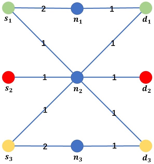
Figure 1: example case

The shortest path method provides a lower bound for the queuing delay. However, the bound can be pretty loose in some cases. Consider a network with the topology shown in Fig. 1. $(s_{1},d_{1}),(s_{2},d_{2})$ and$(s_{3},d_{3})$ are three transmission pairs. Obviously, the shortest path for each pair is the path that goes through node $n_{2}$ of which the propagation delay is 2. When all sources continually send packets to their destination, the shortest path method will provide an unbounded queuing delay, as node $n_{2}$ receives three packets at each time slot, but it can only serve one. However, the actual case should be that most of the packets of $(s_{1},d_{1})$, $(s_{3},d_{3})$ go through $n_{1}$, $n_{3}$ without queuing delay, respectively. Only $s_{2},d_{2}$ suffers from the traffic jam at node $n_{2}$.

The example indicates that the possible detour of the routing should also be considered in approximating the queuing delay. For source-destination pairs that are connected by bottleneck-free routes, a delay estimation is always provided by the detour that is always stable. Such detour can be found using Algorithm 2.

1 given The network $\mathbf{G}=\left(\mathbf{V},\mathbf{E}\right)$, source-destination pair $(s_{i},d_{j}),i=1,2,...,|S|,\ j=1,2,...,|D|$;

2 delete all bottleneck nodes and edges that contains such nodes;

3 for each source-destination pair $(s_{i},d_{j})$ do

4    Use Dijkstra algorithm to find a new path $P^{\prime}_{s_{i}d_{j}}$between $s_{i}$ and $d_{j}$;

5    if $P^{\prime}_{s_{i}d_{j}}$ exists then

6       Record $P^{\prime}_{s_{i}d_{j}}$ as detour path;

7      

8    else

9      Skip to the next pair;

10    end if

11   

12 end for

Algorithm 2 Detour detection algorithm.

As a conclusion, the approximate delay of $(s_{i},d_{j})$ is:

$$D(s_{i},d_{j})=$$ (8)

$$\begin{cases}&D(P_{s_{i}d_{j}})+D(Q_{s_{i}d_{j}})\\ &\ \ \ \ \ \ \mbox{if no detour exists between}\ s_{i},d_{j}\\ &\min\left\{D(R_{s_{i}d_{j}})+D(Q_{s_{i}d_{j}}),\ D(R^{\prime}_{s_{i}d_{j}})+D(Q^{\prime}_{s_{i}d_{j}})\right\}\\ &\ \ \ \ \ \ \ \ \ \ \ \ \ \ \ \ \ \ \ \ \ \ \ \ \ \ \ \ \ \ \mbox{otherwise}\\ \end{cases}$$

where $D(R_{s_{i}d_{j}})$ and $D(R^{\prime}_{s_{i}d_{j}})$ are given by Dijkstra shortest path method, lower bound of $D(Q_{s_{i}d_{j}})$ is given in [8], and $D(Q^{\prime}_{s_{i}d_{j}})$ can be estimated as a tandem M/D/1 queuing system queue.

V Simulation Evaluation

In this section, we evaluate the precision of the delay analysis model introduced in Section III and Section IV. We consider several networks in the evaluation, including different scale random graphs shown in Fig. 2 and the special case shown in Fig. 3.

For the 30 nodes case, both the number of source and destination nodes are 3. While for the 100 nodes case, the number are 10. The topology as well as the weight of each link are generated randomly following Gaussian distribution. Without loss of generality, the source nodes are nodes with smallest serial number, while largest numbers are allocated to destination nodes.

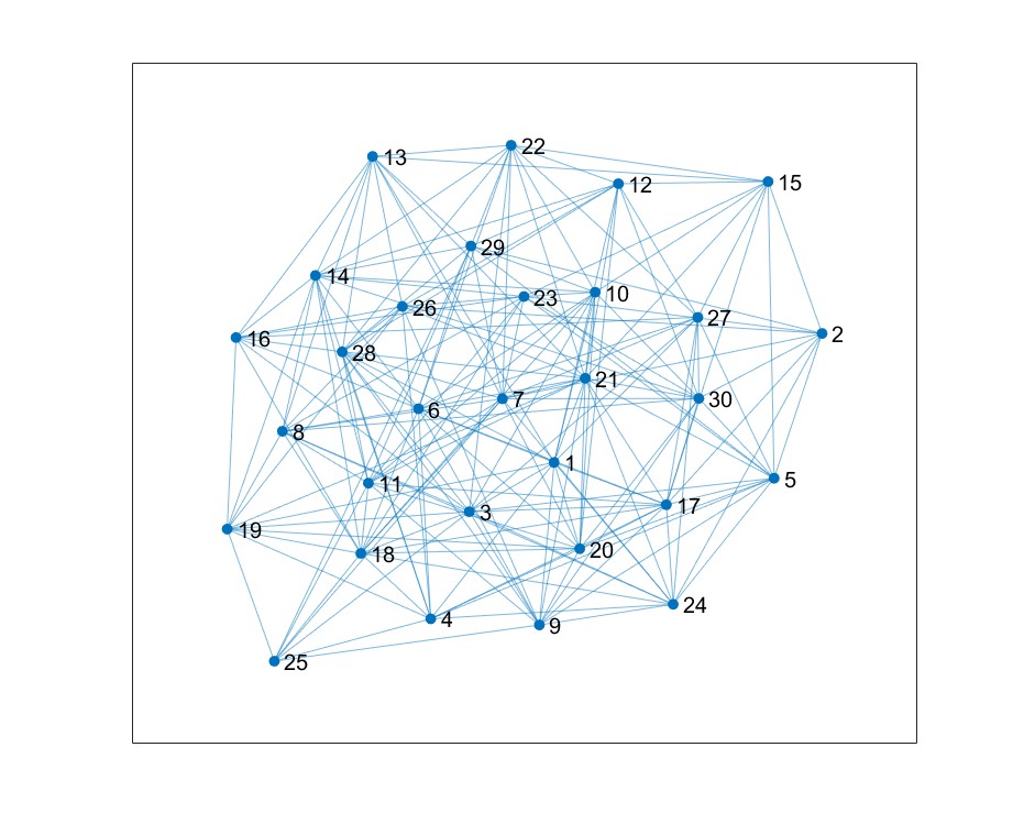
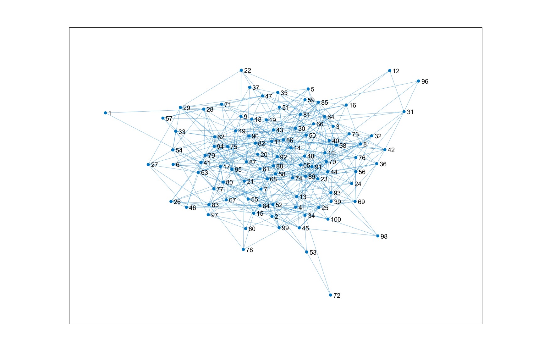
Figure 2: Network topology with (a) 30 nodes (b) 100 nodes.

From Fig. 3. The average packet delay grows with the increase in the packet generation rate $\lambda$. This is because when generation rate becomes larger, more packets are transmitted in the network, causing more severe queuing delays. On the other hand, it is obvious that the lower bound give a good estimation of the average delay.

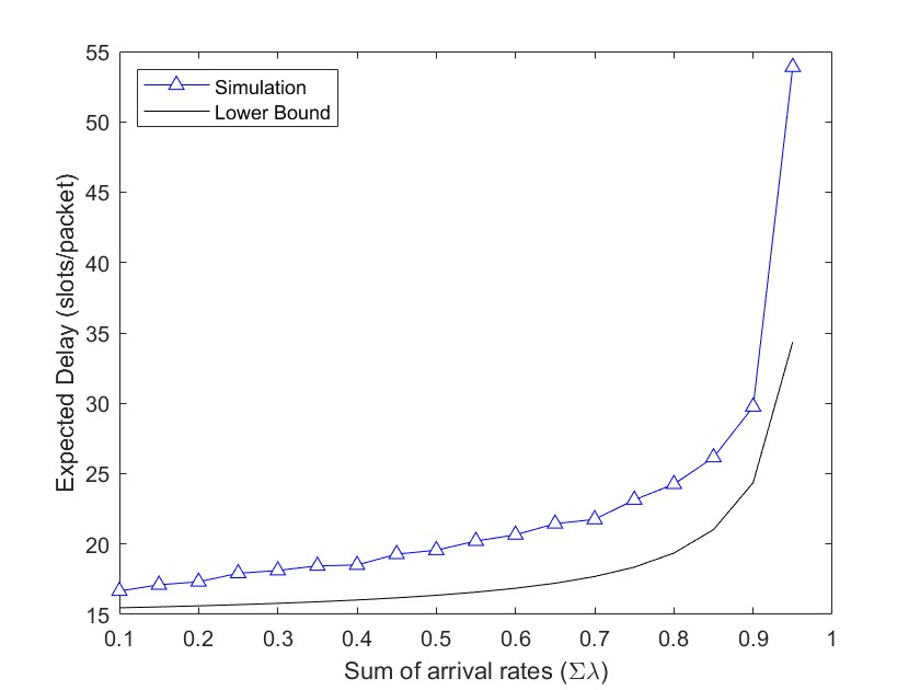
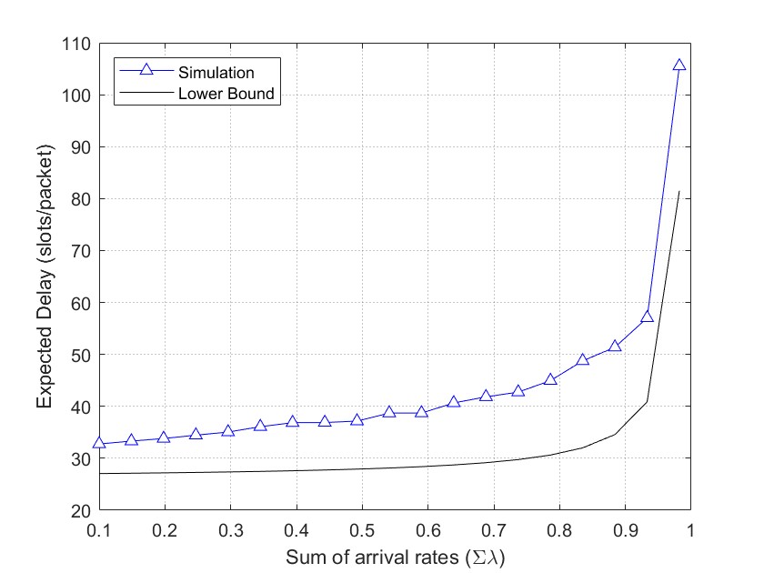
Figure 3: Average packet delay versus sum of arrival rate with (a) n = 30 (b) n = 100.

For the special case, the growth pattern of the average packet delay of ($s_{1}$,$d_{1}$) can be divided into two phases. When the packet generation rate is small, the delay grows with the increase in $\lambda$, as observed in the other cases. However, when the generation rate is large, which means the bottleneck is experiencing heave traffics, the delay is not increasing boundlessly, like what happens in the normal cases. The delay is still very small even the network is unstable (sum of $\lambda$ is greater than 1). On the other hand, the detour method still provide a good track of the average delay as expected.

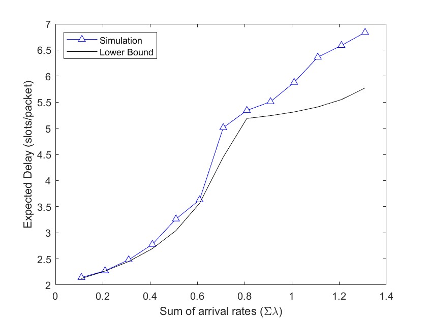
Figure 4: Average packet delay of ($s_{1}$,$d_{1}$) transmission pair versus sum of arrival rate of the special case

VI Conclusion

In this paper, we provide a packet delay analysis for an arbitrary network that has multi sources and destinations when broadcasting through network coding method is applied. We provide a lower bound of the propagation delay as well as the queuing delay for the general cases. For a special sub case, we invented a detour method to provide a more accurate estimation of the delay.

References

- [1] H. Chen, L. Liu, J. D. Matyjas, and M. J. Medley, “Cooperative routing for underlay cognitive radio networks using mutual-information accumulation,” IEEE Transactions on Wireless Communications, vol. 14, no. 12, pp. 7110–7122, 2015.
- [2] T. Ho, M. Medard, R. Koetter, D. Karger, M. Effros, J. Shi, and B. Leong, “A random linear network coding approach to multicast,” IEEE Transactions on Information Theory, vol. 52, no. 10, pp. 4413–4430, 2006.
- [3] T. Ho, R. Koetter, M. Medard, D. Karger, and M. Effros, “The benefits of coding over routing in a randomized setting,” in IEEE International Symposium on Information Theory, 2003. Proceedings., 2003, pp. 442–.
- [4] E. Fasolo, M. Rossi, J. Widmer, and M. Zorzi, “On mac scheduling and packet combination strategies for practical random network coding,” in 2007 IEEE International Conference on Communications, 2007, pp. 3582–3589.
- [5] A. Fujimura, S. Y. Oh, and M. Gerla, “Network coding vs. erasure coding: Reliable multicast in ad hoc networks,” in MILCOM 2008 - 2008 IEEE Military Communications Conference, 2008, pp. 1–7.
- [6] C. Fragouli, J. Widmer, and J.-Y. Le Boudec, “A network coding approach to energy efficient broadcasting: From theory to practice,” in Proceedings IEEE INFOCOM 2006. 25TH IEEE International Conference on Computer Communications, 2006, pp. 1–11.
- [7] H. Song, L. Liu, S. M. Pudlewski, and E. S. Bentley, “Random network coding enabled routing protocol in unmanned aerial vehicle networks,” IEEE Transactions on Wireless Communications, vol. 19, no. 12, pp. 8382–8395, 2020.
- [8] G. R. Gupta and N. B. Shroff, “Delay analysis and optimality of scheduling policies for multihop wireless networks,” IEEE/ACM Transactions on Networking, vol. 19, no. 1, pp. 129–141, 2011.
- [9] Q. Ye, W. Zhuang, X. Li, and J. Rao, “End-to-end delay modeling for embedded vnf chains in 5g core networks,” IEEE Internet of Things Journal, vol. 6, no. 1, pp. 692–704, 2019.
- [10] M. J. Neely, Stochastic Network Optimization with Application to Communication and Queueing Systems. Morgan and Claypool Publishers, 2010.