The spectra of solar magnetic energy and helicity

Abstract

Previous studies have used magnetic energy and helicity spectra, the latter computed using the two-scale method, to search for signatures of mean-field dynamos. In this study, we compare cotemporal HMI and SOLIS magnetograms to illustrate the instrument-dependence of even qualitative features of the energy and helicity spectra. Around the minimum between solar cycles 24 and 25, we find that the magnetic energy spectrum computed from HMI observations exhibits two distinct peaks. One of these peaks is only present near the cycle minimum, and corresponds to large-scale magnetic fields at high latitudes. Nevertheless, such magnetic fields are not present in contemporaneous synoptic vector magnetograms from SOLIS. Further, even when magnetograms from both the instruments are apodized, the helicity spectra calculated using the two-scale method disagree (on both the sign and the value of the fractional helicity). This suggests that currently available synoptic magnetograms are not reliable enough for such studies.

1 Introduction

The Sun exhibits a magnetic cycle that is roughly 22 years long, along with a correlated 11-year sunspot cycle (Hathaway, 2015). While the factors determining the strength and the periodicity of the solar magnetic field are a matter of debate, most proposed explanations appeal to dynamos of some kind or the other (Charbonneau, 2020).

Magnetic helicity (a measure of the topological linkage between magnetic field lines) is conserved in ideal magnetohydrodynamics; further, the rate of its dissipation approaches zero in the astrophysically relevant limit of large magnetic Reynolds number (Brandenburg & Subramanian, 2005, section 3.4; Pariat et al., 2015). It thus plays a crucial role in mean-field dynamo theory.

The kinetic helicity in the Sun is theoretically expected to be negative in the northern hemisphere and to flip sign across the equator (Roberts & Stix, 1971, p. 156). For a large-scale magnetic field generated exclusively through the $\alpha$ effect, one expects the sign of the associated magnetic helicity to be the opposite of that of the kinetic helicity. The resulting change in the sign of the large-scale magnetic helicity across the equator is referred to as the hemispheric sign rule (HSR). Further, in such a scenario, the small- and large-scale fields in a particular hemisphere are expected to have magnetic helicities of opposite signs, such that the magnetic helicity of the total magnetic field in a particular hemisphere is close to zero (see Brandenburg & Subramanian, 2005, eqs. 9.11, 9.12). On the other hand, in a mean-field model that also includes differential rotation, Pipin et al. (2013) found reversals of the HSR near cycle minima. The spatial and spectral distribution of the magnetic helicity is thus a source of information on which dynamo mechanisms contribute to the solar magnetic cycle.

One way to observationally test the HSR is to use the helicity of the electric current in active regions as a proxy for the magnetic helicity therein. Applying this method to observations of a number of active regions, Seehafer (1990) and Zhang et al. (2010) found latitudinal sign changes corresponding to those expected for the small-scale magnetic helicity.

Another approach, first used by Brandenburg et al. (2003), is to calculate the magnetic helicity of the axisymmetric part of the solar magnetic field from the longitudinal average of observed synoptic magnetograms. Using a similar technique, Pipin & Pevtsov (2014) found that the helicity of the axisymmetric part of the magnetic field obeys the HSR corresponding to large-scale fields. They also found that while the magnetic and current helicities of the large-scale fields show broadly similar latitudinal trends, they differ in detail.

Pipin et al. (2019), who computed the helicity densities of both the axisymmetric and non-axisymmetric parts of the magnetic field, found that while the axisymmetric part behaves as expected for a large-scale field, the non-axisymmetric part does not consistently display the behaviour expected from the HSR for a small-scale field (i.e., the helicities of the axisymmetric and non-axisymmetric parts are occasionally of the same sign).

While the studies mentioned above considered any non-axisymmetric part of the magnetic field as a small-scale component, a more nuanced approach based on the helicity spectrum was used by Zhang et al. (2014). Computing the magnetic helicity spectrum over a single active region, they found a sign consistent with the HSR at large scales. Applying the same method to thousands of active regions, Gosain & Brandenburg (2019) found that individual active regions only obey the HSR poorly.

A complication in calculating global helicity spectra (as opposed to spectra over isolated active regions) is that the expected sign change of the helicity across the equator would lead to the helicity spectrum being zero at each wavenumber if calculated over the entirety of the Sun’s surface. To capture the expected sign change across the equator, Brandenburg et al. (2017) applied a ‘two-scale’ method to synoptic magnetograms in order to calculate energy and helicity spectra. They used a Cartesian approximation to facilitate the application of Fourier transforms. Prabhu et al. (2021) have described a similar method that uses spherical harmonics, and shown that the results are similar to those obtained in the Cartesian approximation. We will thus continue to use the Cartesian approximation in this work.

Comparing synoptic magnetograms from different facilities (including HMI, MDI, and SOLIS), Riley et al. (2014) found that conversion factors between the line-of-sight magnetic fields measured by different instruments can be latitude-dependent, and even time-dependent. Such differences are expected to affect the energy and helicity spectra. Further, comparing synoptic magnetograms from HMI and MDI, Luo et al. (2023) have found that the energy spectra can only be matched by applying a scale-dependent correction factor. Due the theoretical importance of the sign of the helicity spectrum, one would like to understand how strongly it is affected by such instrument-dependent effects.

Dividing full-disk vector magnetograms from the Huairou Solar Observing Station into strong-field ($\left|B_{\textsc{LOS}}\right|>\qty{1000}{G}$, where $B_{\textsc{LOS}}$ is the line-of-sight component of the magnetic field) and weak-field ($\qty{100}{G}<\left|B_{\textsc{LOS}}\right|<\qty{500}{G}$) parts and analysing them separately, Zhang (2006) found that their current helicities are of opposite signs, with the weak fields obeying (only in a statistical sense) the HSR corresponding to small-scale fields. On the other hand, GosPevRud13, who performed a similar study using SOLIS synoptic vector magnetograms, arrived at the conclusion that it is the strong fields that obey the HSR corresponding to small-scale fields, with the weak field regions having current helicities of the opposite sign. One possible explanation for this disagreement is that one or both of these observations are affected by instrument-dependent systematic biases. Another possible explanation is that biases introduced during the assembly of synoptic magnetograms affect inferences of the magnetic helicity and its proxies.

Using the two-scale method in the Cartesian approximation, Singh et al. (2018) have found that during Carrington rotations 2161--2163, the sign of the helicity spectrum as computed from SOLIS synoptic magnetograms disagrees with that computed from HMI synoptic magnetograms. However, it is unclear whether this particular interval of time is an aberration, or if helicity spectra computed from synoptic magnetograms using the two-scale method are always instrument-dependent.

Our main goal in this study is to compare the helicity spectra computed from HMI and SOLIS synoptic magnetograms in Carrington rotations 2097--2195 (slightly more than 7 years), and check how well they agree. In the process, we clarify various implementation details and correct errors in previous applications of the two-scale method. We also show that around the solar minimum, discrepancies in the polar fields are strong enough to qualitatively change even the magnetic energy spectrum.

Section 2 describes the two-scale method. Since previous implementations of the two-scale method had various errors, we verify our implementation applying it to simulations in section 3. Section 4 gives the details of the data we have used and our analysis procedure. In section 5, we show that near the minimum between solar cycles 24 and 25, one can find large-scale magnetic fields at high latitudes in HMI synoptic magnetograms, but not in cotemporal SOLIS synoptic magnetograms. Section 6 shows that even when the high latitudes are removed, the helicity spectra calculated from HMI and SOLIS synoptic magnetograms do not agree. We show that agreement is bad throughout the time interval in which data are available from both the instruments. Finally, section 7 summarizes our conclusions. The scripts used for this study, along with the input files for the simulations, have been archived on Zenodo (Kishore & Singh, 2025); alternatively, they can be downloaded from https://github.com/Kishore96in/bihelical-mag-fields.

2 Description of the two-scale method

2.1 Locally isotropic, weakly inhomogeneous turbulence

Let us consider the Fourier-space two-point correlation function of the magnetic field:

$$M_{ij}(\boldsymbol{k},\boldsymbol{K})\equiv\left<B_{i}{\left(\boldsymbol{k}+\tfrac{1}{2}\,\boldsymbol{K}\right)}\,B_{j}^{*}{\left(\boldsymbol{k}-\tfrac{1}{2}\,\boldsymbol{K}\right)}\right>$$ (1)

For turbulence that is locally isotropic and weakly inhomogeneous (Moffatt, 1978, eq. 7.56; Lesieur, 2008, eq. 5.84), we can write the spectra of the magnetic energy and the magnetic helicity as

$$\begin{split}8\pi M(k,K)={}&\int M_{ii}(\boldsymbol{k},\boldsymbol{K})\,\mathrm{d}\Omega_{k}\end{split}$$ (2)

$$\begin{split}8\pi N(k,K)={}&\int ik_{i}\epsilon_{ijk}\,M_{jk}(\boldsymbol{k},\boldsymbol{K})\,\mathrm{d}\Omega_{k}\end{split}$$ (3)

respectively. The quantities $M$ and $N$ are related to the quantities $\widetilde{E}_{M}$ and $\widetilde{H}_{M}$ (defined by Zhang et al., 2014; Brandenburg et al., 2017; and Singh et al., 2018) by

$$\begin{split}\widetilde{E}_{M,\text{3D}}(k,\boldsymbol{K})={}&4\pi k^{2}\,M(k,\boldsymbol{K})\end{split}$$ (4a)

$$\begin{split}={}&\frac{1}{2}\int M_{ii}(\boldsymbol{k},\boldsymbol{K})\,k^{2}\,\mathrm{d}\Omega_{k}\end{split}$$ (4b)

$$\begin{split}\widetilde{H}_{M,\text{3D}}(k,\boldsymbol{K})={}&8\pi\,N(k,\boldsymbol{K})\end{split}$$ (4c)

$$\begin{split}={}&\int i\,\epsilon_{ijk}\,\frac{k_{i}}{k^{2}}\,M_{jk}(\boldsymbol{k},\boldsymbol{K})\,k^{2}\,\mathrm{d}\Omega_{k}\end{split}$$ (4d)

Note that the magnetic energy and the magnetic helicity are proportional to $\int\widetilde{E}_{M,\text{3D}}\ \mathrm{d}k$ and $\int\widetilde{H}_{M,\text{3D}}\,\mathrm{d}k$ respectively.

2.2 Definitions of the energy and helicity spectra

While our reasoning so far has been in terms of the continuous Fourier transform, it is conventional in observational work to use the discrete Fourier transform. If we define $M_{ij}$ (equation 1) in terms of the discrete Fourier transform of the magnetic field, we find that it has the same dimensions as the square of the magnetic field. Analogous to equations 4, we define the energy and helicity spectra as

$$\begin{split}\widetilde{E}(k,\boldsymbol{K})\equiv{}&\sum_{\boldsymbol{q}}\frac{1}{2}\,M_{ii}(\boldsymbol{q},\boldsymbol{K})\operatorname{\mathds{1}}(\boldsymbol{q},k)\end{split}$$ (5)

$$\begin{split}\widetilde{H}(k,\boldsymbol{K})\equiv{}&\sum_{\boldsymbol{q}}i\,\epsilon_{ijk}\,\frac{q_{i}}{q^{2}}\,M_{jk}(\boldsymbol{q},\boldsymbol{K})\operatorname{\mathds{1}}(\boldsymbol{q},k)\end{split}$$ (6)

where $\operatorname{\mathds{1}}(\boldsymbol{q},k)$ is one when $-\Delta/2\leq\left|\boldsymbol{q}\right|-k<\Delta/2$, and zero elsewhere ($\Delta$ is the spacing between adjacent values of $k$); note that this indicator function has replaced the 3D angular element $k^{2}\,\mathrm{d}\Omega_{k}$. Note that $\widetilde{E}$ and $k\widetilde{H}$ have units of $\mathrm{G}^{2}$, which is equivalent to $\mathrm{e}\mathrm{r}\mathrm{g}\,\mathrm{c}\mathrm{m}^{-3}$.

2.3 Extension to 2D

In principle, the expressions above are not directly applicable to solar magnetograms, since they require information about the magnetic field in a three-dimensional volume. Zhang et al. (2014, p. 3) and Brandenburg et al. (2017, p. 2) heuristically derived their expressions by making the replacement $4\pi k^{2}\,\mathrm{d}\Omega_{\text{3D}}\to 2\pi k\,\mathrm{d}\Omega_{\text{2D}}$ in equations 4. Similarly, we use equations 5 and 6, but with the sum over $\boldsymbol{q}$ restricted such that the component of $\boldsymbol{q}$ out of the plane is zero (i.e. we only sum over wavevectors lying within the plane).

2.4 The important part of the helicity spectrum

According to the HSR, the large-scale magnetic fields have helicities of opposite signs in the northern and southern hemispheres. If one is searching for signs of large-scale dynamo action, one should thus look at the part of the large-scale helicity that changes sign about the equator. An example of such a function is $\sin(2\lambda)$, with $\lambda$ being the latitude in radians. Recalling the Fourier transform

$$\sin(\boldsymbol{K}_{1}\cdot\boldsymbol{X})\to\frac{1}{2i}\left[\operatorname{\delta}{\!\left(\boldsymbol{K}-\boldsymbol{K}_{1}\right)}-\operatorname{\delta}{\!\left(\boldsymbol{K}+\boldsymbol{K}_{1}\right)}\right]$$ (7)

we find that the part of the helicity spectrum that corresponds to such a modulation has a large-scale wavevector $\boldsymbol{K}_{1}\equiv 2\pi\boldsymbol{\hat{\lambda}}/L_{\lambda}$. Further, to obtain the contribution proportional to this with a sign corresponding to the sign of the helicity in the northern hemisphere, one has to take the negative imaginary part of $\widetilde{H}(k,\boldsymbol{K}_{1})$.

3 Verification of the two-scale method

Brandenburg et al. (2017) attempted to verify their implementation of the two-scale method by applying it to slices saved from a simulation. Examination of the script they used to create their figure 6b suggests that what they plot is actually the positive imaginary part of the helicity spectrum (and not the relevant negative imaginary part as claimed). We now check if the two-scale method remains valid once this (and another mistake which we will point out in due course) is corrected.

Our simulation setup is similar to that used by [sec. 3.2]BraPetSin17. We consider isothermal turbulence in a periodic cube of size $2\pi$ length units in each direction. The velocity field is forced by linear combinations of the eigenfunctions of curl operator, chosen to have a prescribed fractional helicity (see Brandenburg, 2001; Haugen et al., 2004), with the helicity switching sign across $z=0$ (the midplane) if necessary. The wavevector of the forcing function is randomly chosen at each timestep to be in the shell $9.5\leq k<10.5$. The evolution equations are solved using the Pencil code (Pencil Code Collaboration et al., 2021). The spatial discretization uses $512^{3}$ points and a sixth-order finite difference scheme. The equations are evolved in time using a third-order Runge-Kutta method. Upwinding is used for advection of the density, the velocity, and the magnetic vector potential (Dobler et al., 2006, appendix B).

Given the magnetic field at a particular instant of time, we consider its values in a single $yz$ plane, and calculate the energy and helicity spectra. This coordinate system is similar to the one we will later use for synoptic maps (section 4.2).

3.1 No sign change of helicity

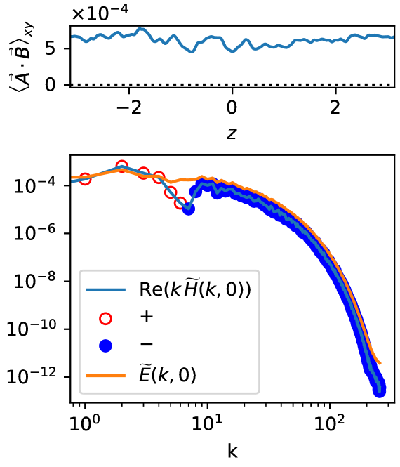
Figure 1: Recovery of the correct sign of the helicity from a simulation where there is no sign change across $z=0$. The helicity in the top panel, calculated directly from $\boldsymbol{A}$ and $\boldsymbol{B}$, has been averaged over $x$ and $y$. The helicity spectrum in the bottom panel is the average of the spectra calculated from $\boldsymbol{B}$ in six $yz$ planes. None of the quantities has been averaged over time.

First, we consider a case where the sign of the helical forcing is the same throughout the domain. In this case, we are interested in the real part of the $K=0$ part of the helicity spectrum. Figure 1 shows that we recover the correct sign of the helicity spectrum (the sign of the mean helicity in the left panel is consistent with the sign in the low-wavenumber region of the right panel).

3.2 Helicity changing sign across the equator

Next, we consider a case where the helicity flips sign across $z=0$, and the domain itself has extent $-L_{z}/2<z<L_{z}/2$. In this case, we expect the strongest contribution to be proportional to $\sin(2\pi z/L_{z})$ (see section 2.4).

3.2.1 The problem

Formally, the expressions for the energy and helicity spectra (equations 5 and 6) involve $M_{ij}(\boldsymbol{k},\boldsymbol{K})\equiv\left<B_{i}{\left(\boldsymbol{k}+\tfrac{1}{2}\,\boldsymbol{K}\right)}\,B_{j}^{*}{\left(\boldsymbol{k}-\tfrac{1}{2}\,\boldsymbol{K}\right)}\right>$. If one wishes to recover a mode with $K_{z}=2\pi/L_{z}$, a problem arises: $2\pi/L_{z}$ is the smallest wavenumber present in the domain, and so it is difficult to make sense of $\boldsymbol{K}/2$.

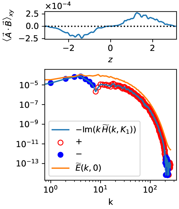
Figure 2: Recovery of the wrong sign of the helicity when one takes $M_{ij}(\boldsymbol{k},\boldsymbol{K})\equiv\left<\widetilde{B}_{i}{\left(\boldsymbol{k}+\boldsymbol{K}\right)}\,\widetilde{B}_{j}^{*}{\left(\boldsymbol{k}\right)}\right>$. The helicity in the top panel, calculated directly from $\boldsymbol{A}$ and $\boldsymbol{B}$, has been averaged over $x$ and $y$. The helicity spectrum in the bottom panel is the average of the spectra calculated from $\boldsymbol{B}$ in six $yz$ planes. None of the quantities has been averaged over time.

3.2.2 The wrong method

To circumvent this issue, BraPetSin17 and SinKapBra18 treat the quantity $\left<\widetilde{B}_{i}{\left(\boldsymbol{k}+\boldsymbol{K}\right)}\,{B}_{j}^{*}{\left(\boldsymbol{k}\right)}\right>$ as being equivalent to $M_{ij}(\boldsymbol{k},\boldsymbol{K})$. If one uses this definition, another mistake (appendix A.1) needs to be made to recover the correct sign of the helicity spectrum. In figure 2, we show that the wrong sign of the helicity is recovered using this method (the sign of the mean helicity in the $z>0$ region on the left panel is inconsistent with the sign in the low-wavenumber region of the right panel).

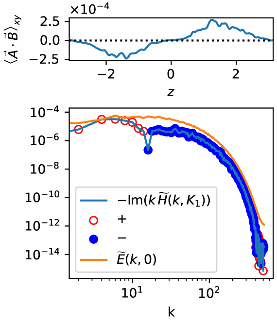
Figure 3: Recovery of the correct sign of the helicity when one takes $M_{ij}(\boldsymbol{k},\boldsymbol{K})\equiv\left<\widetilde{B}_{i}{\left(\boldsymbol{k}+\boldsymbol{K}/2\right)}\,\widetilde{B}_{j}^{*}{\left(\boldsymbol{k}-\boldsymbol{K}/2\right)}\right>$. The helicity in the top panel, calculated directly from $\boldsymbol{A}$ and $\boldsymbol{B}$, has been averaged over $x$ and $y$. The helicity spectrum in the bottom panel is the average of the spectra calculated from $\boldsymbol{B}$ in six $yz$ planes after doubling the extent of the domain as described in the text. None of the quantities has been averaged over time.

3.2.3 The correct method

An alternative is to double the length of the domain (keeping the equator, if any, still at the middle); this is consistent with the assumption of periodicity that goes into expanding a function (in a finite domain) as a Fourier series. In this particular case, we extend the definition of $\boldsymbol{B}$ as (omitting the other arguments for brevity)

$$\boldsymbol{B}(z)=\begin{dcases}\boldsymbol{B}(z+L_{z})\,,&-L_{z}\phantom{/2}<z<-L_{z}/2\\ \boldsymbol{B}(z)\,,&-L_{z}/2<z<\phantom{-}L_{z}/2\\ \boldsymbol{B}(z-L_{z})\,,&\phantom{-}L_{z}/2<z<\phantom{-}L_{z}\end{dcases}$$ (8)

To keep the spacing between the wavevectors the same in both the directions, we also double the domain along the $y$ direction (recall that the domain was initially cubical). After calculating the spectra, we rebin them in terms of the wavenumbers of the original domain (since doubling the domain halves the spacing between the wavenumbers). In figure 3, we show that this method allows us to recover the correct sign of the helicity spectrum.

4 Data analysis

4.1 The magnetograms used

4.1.1 HMI

HMI is an instrument on SDO (Solar Dynamics Observatory, a geosynchronous satellite) which observes the $617.3\text{\,}\mathrm{n}\mathrm{m}$ line of Fe i in absorption. After computing the Stokes parameters from these measurements, the vector magnetic field on the observed solar disk is obtained using a Milne-Eddington-based inversion algorithm. Azimuth disambiguation is done using the minimum-energy algorithm in strong-field ($\left|\boldsymbol{B}\right|>\qty{150}{G}$) regions, while the sign of the transverse component is randomly assigned in weak-field regions. Synoptic maps are then constructed by, for each combination of Carrington longitude and latitude, averaging over magnetograms where that particular location is closest to the observed central meridian. Liu et al. (2017) describe the production of both full-disk and synoptic vector magnetograms in more detail.

We use $360\times 720$ pixel (sine-latitude vs longitude) vector synoptic maps (series b_synoptic_small) downloaded from JSOC. We rebin these using cubic spline interpolation to a grid equispaced in latitude, preserving the number of pixels.

4.1.2 SOLIS

SOLIS’s VSM (Vector Spectro-Magnetograph) observes a pair of Fe i lines around 630.2nm in absorption (Keller et al., 2003, section 2). The vector magnetic field is obtained from the Stokes parameters using a Milne-Eddington-based inversion algorithm (Harker, 2017). Azimuthal disambiguation has supposedly been done using the ‘Very Fast Disambiguation method’ proposed by RudAnf14. Synoptic maps are constructed by averaging over multiple magnetograms, with a weighting factor ensuring that the dominant contributions to a particular Carrington longitude come from magnetograms where that longitude is near the central meridian. We use $180\times 360$ pixel (latitude vs longitude) vector synoptic maps.

4.2 Coordinate system and domain

Using $\boldsymbol{\hat{r}}$, $\boldsymbol{\hat{\theta}}$, and $\boldsymbol{\hat{\phi}}$ to denote the radial, colatitudinal, and azimuthal unit vectors on the Sun’s surface, we note that $\boldsymbol{\hat{r}}$, $\boldsymbol{\hat{\phi}}$, and $\boldsymbol{\hat{\theta}}$ form a left-handed coordinate system. A right-handed coordinate system can then be formed by taking one’s unit vectors as $\boldsymbol{\hat{r}}$, $\boldsymbol{\hat{\phi}}$, and $\boldsymbol{\hat{\lambda}}$, where $\boldsymbol{\hat{\lambda}}\equiv-\boldsymbol{\hat{\theta}}$. The components of the magnetic field are given by $(B_{r},B_{\phi},B_{\lambda})=(B_{r},B_{\phi},-B_{\theta})$ (Brandenburg et al., 2017, eq. 20; Singh et al., 2018, eq. 10).

We unwrap the surface of the Sun to form a Cartesian 2D domain, such that the position vector is $\boldsymbol{X}=(X_{\phi},X_{\lambda})$; and the domain has size $L_{\phi}\times L_{\lambda}=2\pi R_{\sun}\times\pi R_{\sun}$ (where $\lambda\equiv\pi/2-\theta$ is the latitude). As discussed in section 2.4, the large-scale wavevector we are interested in is then $\boldsymbol{K}_{1}\equiv 2\pi\boldsymbol{\hat{\lambda}}/L_{\lambda}$.

4.3 Averaging

Recall that the two-point correlation of the magnetic field (equation 1) is defined as an average. In the context of this work, the magnetic field used to calculate the two-point correlations is from synoptic vector magnetograms, and the averaging is over the azimuthal large-scale coordinate (due to our choice of the large-scale wavevector), the angular part of the small-scale coordinate, and time.

The magnetic field in a synoptic magnetogram may itself be thought of as an average over multiple full-disk observations, meaning that some information on the two-point correlations is lost in the process of creating synoptic magnetograms. Exploring how this affects the calculated spectra is left to future work.

4.4 Error estimates

Spectra calculated from single magnetograms are expected to be affected by stochastic fluctuations. To suppress these fluctuations, we average spectra over a number of contiguous magnetograms. We then estimate the stochastic errors in these averaged spectra by using the jackknife method: given $N$ realizations of a random variable $X$ (denoted by $X_{1},\dots X_{N}$), the error in their mean is estimated as the standard deviation of $\mu_{1},\dots\mu_{N}$, where

$$\mu_{i}\equiv\sum_{\begin{subarray}{c}j=1\\ j\neq i\end{subarray}}^{N}\frac{X_{j}}{N-1}$$ (9)

The procedure chosen for azimuth disambiguation is expected to affect the helicity spectrum. In particular, for the HMI magnetograms, the sign of the transverse field is randomly chosen in weak-field regions. Since the random signs chosen for different magnetograms are uncorrelated, the error estimated using equation 9 also includes the error due to this specific disambiguation procedure. We show this in appendix B. However, note that our error estimate does not include the error due to other disambiguation methods (e.g. the minimum energy algorithm used for the HMI magnetograms in strong-field regions).

No attempt is made to estimate other sources of systematic error, e.g. due to the model atmospheres used in the inversion process.

5 Signs of polar fields in magnetic energy spectra

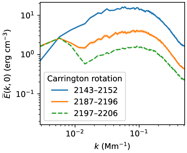
Figure 4: Energy spectra calculated from HMI magnetograms, averaged over the indicated Carrington rotations. Errors are indicated by shaded regions of the same colour as the corresponding lines, but are too small to be clearly visible.

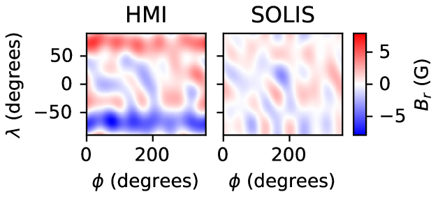
Figure 5: Low-pass-filtered ($k<\qty{e-2}{Mm^{-1}}$) synoptic HMI and SOLIS maps of the radial magnetic field in Carrington rotation 2180 (30-Jul-2016 -- 26-Aug-2016).

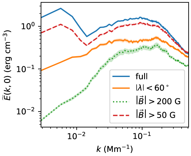
Figure 6: The effect, of removing high latitudes or weak-field regions from HMI magnetograms, on the magnetic energy spectrum (averaged over Carrington rotations 2197--2206). The legend indicates which region of each magnetogram was used to compute the spectrum.

Figure 4 shows the magnetic energy spectra calculated from HMI synoptic vector magnetograms at different phases of solar cycle 24. Near the peak of solar cycle 24 (Carrington rotations 2143--2152), we find that the magnetic energy spectrum peaks at a single scale. However, closer to the minimum between cycles 24--25, we find that the magnetic energy spectrum has a second peak at around 6e-3Mm^-1.

Let us now investigate what exactly these large-scale features correspond to. The left panel of figure 5 shows a low-pass-filtered HMI synoptic map from a single Carrington rotation (2180). The large-scale features we saw in the spectra show up as a dipolar component, strongest at latitudes $\left|\lambda\right|>$$$. The sign of this large-scale dipolar field is consistent with that expected for the polar fields at this stage of the solar cycle (see Hathaway, 2015, figure 17).

The right panel of figure 5 shows a low-pass-filtered SOLIS magnetogram. While the magnetograms from HMI and SOLIS are comparable near the equator, they are completely different at high latitudes. In particular, the SOLIS magnetograms do not have a prominent dipolar component at high latitudes. Given the complex process through which synoptic magnetograms are derived from line profiles, it is difficult to immediately point out why the two magnetograms differ so drastically.

Vector magnetograms are considered unreliable at high latitudes (e.g. Brandenburg et al., 2017, p. 5; Luo et al., 2023, p. 2) and in regions where the magnetic field is weak. The former is related to projection effects, while the latter is due to magnetic effects on the observed lines being overpowered by noise. The simplest way of obtaining results that do not depend on these regions is to set the magnetic field to zero there. Apodization refers to removing the effect of high-latitude regions by either setting them to zero or using some sort of windowing function. In figure 6, we show that the peak at low wavenumbers is suppressed when the magnetic field is set to zero either at high latitudes or in weak-field regions.

Many studies (e.g. Brandenburg et al., 2017; Pipin et al., 2019) use magnetograms without any special treatment of the high-latitude regions; one expects such studies to be affected by the instrument-dependence of the strength of the polar fields. On the other hand, there are also more complicated approaches that involve using an extrapolation scheme to fill in the data at high latitudes (e.g. Luo et al., 2023, p. 2), which we do not explore here.

6 Disagreement between helicity spectra from cotemporal HMI and SOLIS magnetograms

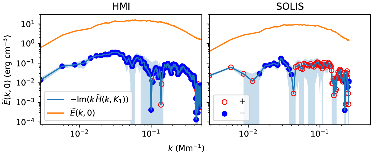
Figure 7: Magnetic energy and helicity spectra calculated from apodized ($\left|\lambda\right|<$$$) HMI and SOLIS magnetograms, averaged over Carrington rotations 2143--2153. Errors have been indicated by shaded regions of the same colour as the corresponding lines.

Despite the issues we noted at large scales, one may still hope that the magnetograms are more reliable at high wavenumbers (which are presumably dominated by active regions, where the strength of the magnetic field allows more accurate inversions). Figure 7 compares energy and helicity spectra from apodized ($\left|\lambda\right|<$$$) HMI and SOLIS magnetograms (Carrington rotations 2143--2153). As noted by SinKapBra18, we find that the sign of the helicity spectrum is instrument-dependent. While the interval compared by [fig. 9]SinKapBra18 (Carrington rotations 2160--2162) showed disagreement between HMI and SOLIS only at the largest wavenumbers, the particular interval we have compared here shows disagreement at both large and small wavenumbers.

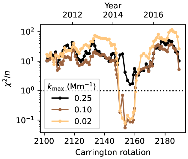
Figure 8: Reduced $\chi^{2}$ statistic (equation 10) as a function of the Carrington rotation, showing that the differences between spectra from HMI and SOLIS magnetograms are much larger than the estimated errors. In each line, only wavenumbers below the indicated cutoff are summed over (the number of such wavenumbers, denoted by $n$, is used to normalize the statistic). The cutoff for the black line, 0.25Mm^-1, is the Nyquist wavenumber for spectra calculated from the SOLIS synoptic magnetograms.

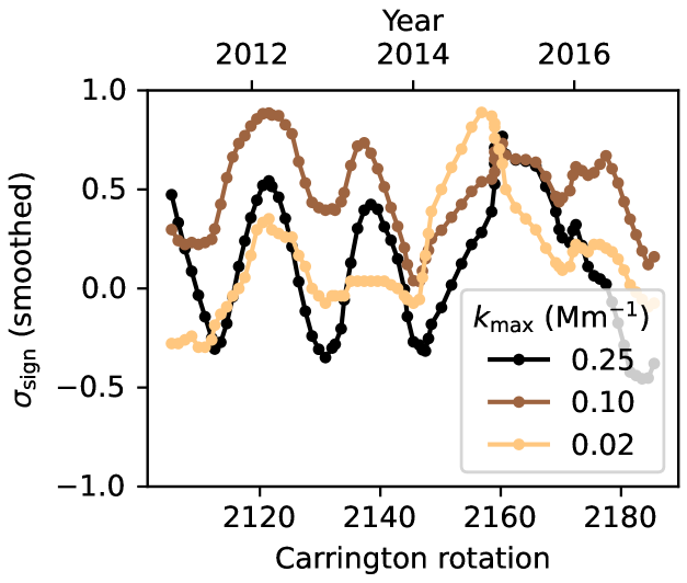
Figure 9: Similar to figure 8, but for the $\sigma_{\text{sign}}$ statistic (equation 11). In this plot, $\sigma_{\text{sign}}$ is smoothed with a boxcar of width 9 Carrington rotations. We see that even the sign of the helicity spectrum is not consistently the same when computed from HMI and SOLIS magnetograms.

To check if this instrument-dependence is consistent with the estimated errors in the helicity spectra, we compute the following statistic:

$$\chi^{2}\equiv\sum_{k}\frac{\left(f_{H}(k)-f_{S}(k)\right)^{2}}{\Delta_{H}^{2}(k)+\Delta_{S}^{2}(k)}$$ (10)

where $f(k)\equiv-k\operatorname{Im}(\widetilde{H}(k,K_{1}))/\widetilde{E}(k,0)$ is the scale-dependent fractional helicity; the subscripts $H$ and $S$ indicate the use of HMI and SOLIS data respectively; and $\Delta$, the error in $f$, is estimated by propagating the estimated errors in $\widetilde{H}(k,K_{1})$ and $\widetilde{E}(k,0)$. Figure 8 shows this quantity as a function of the Carrington rotation. The spectra and errors that determine $\chi^{2}$ are calculated using a rolling window of width 10 Carrington rotations, and the Carrington rotation attributed to a particular window is the average of the Carrington rotations of all the contributing synoptic magnetograms. We use synoptic magnetograms for Carrington rotations 2097 through 2195 (this being the interval in which synoptic magnetograms are available from both HMI and SOLIS). Carrington rotations 2099, 2107, 2127, 2139, 2152, 2153, 2154, 2155, 2163, 2164, 2166, 2167, and 2192 are excluded, since the corresponding SOLIS magnetograms suffer from poor data coverage.

We see that throughout the time period under consideration, the differences between the fractional helicity spectra from HMI and SOLIS synoptic magnetograms are much larger than the errors we have estimated. If only large wavenumbers ($k<\qty{0.1}{Mm^{-1}}$) are considered, the agreement is similarly bad, except in Carrington rotations 2150--2160 (roughly May 2014 -- February 2015). It is unclear what is special about this interval of time; no changes in the versioning keywords of the HMI or SOLIS magnetograms seem to coincide with it.

Since the sign of the helicity spectrum is itself of theoretical importance, we also consider another quantity that tells us if at least both instruments predict consistent signs for the helicity spectrum (ignoring any differences in its magnitude):

$$\sigma_{\text{sign}}\equiv\left<\operatorname{sgn}_{\Delta}[\operatorname{Im}(\widetilde{H}_{H}(k,K_{1}))]\operatorname{sgn}_{\Delta}[\operatorname{Im}(\widetilde{H}_{S}(k,K_{1}))]\right>_{k}$$ (11)

where

$$\operatorname{sgn}_{\Delta}(x)\equiv\begin{dcases}-1\,,&\phantom{-\Delta_{x}<{}}x<-\Delta_{x}\\ \phantom{-{}}0\,,&-\Delta_{x}<x<\phantom{-{}}\Delta_{x}\\ \phantom{-{}}1\,,&\phantom{-{}}\Delta_{x}<x\end{dcases}$$ (12)

with $\Delta_{x}$ being the error in $x$. Figure 9 shows that even this quantity (computed using the same magnetograms as above, and further smoothed temporally to bring out broad trends) is not consistently high.

7 Conclusions

While the two-scale method introduced by BraPetSin17 may allow one to extract much more information from magnetograms than competing methods, it has certain subtle implementation issues which were not discussed in the original papers. To aid application of this method, we have discussed these problems and their solutions.

Application of this method to HMI synoptic vector magnetograms reveals that throughout the solar cycle, the magnetic energy spectrum peaks at a wavenumber of roughly 0.1Mm^-1. Near the cycle minimum, a second peak appears at a lower wavenumber, corresponding to Sun’s well-known polar fields. However, somewhat surprisingly, these polar fields are not prominent in cotemporal SOLIS synoptic vector magnetograms. Previous applications of the two-scale method (Brandenburg et al., 2017; Singh et al., 2018) used magnetograms from the declining phase of solar cycle 24, and hence this discrepancy was not noticed.

Even after excluding high-latitude regions where the magnetograms are expected to be unreliable, comparison of the helicity spectra computed using the two-scale method reveals that in general, the SOLIS and HMI data differ on both the sign of the magnetic helicity spectrum and the value of the fractional magnetic helicity at all scales. The helicity spectra at large wavenumbers agree well only in the interval of time between Carrington rotations 2150--2160, which is in the early part of the declining phase of solar cycle 24. It is unclear if this is just a coincidence.

Part of the disagreement between HMI and SOLIS could, in principle, be attributed to the fact that they observe different spectral lines. However, the differences between the respective contribution functions are comparable to their widths and to changes due to the presence of a magnetic field --- see Faurobert et al. (2009) and Grec et al. (2010) for the formation heights of the lines used by SOLIS; Holzreuter & Solanki (2012, fig. 7) for magnetic effects on these lines; and Norton et al. (2006, table 1) and Fleck et al. (2011, fig. 11) for the formation height of the line used by HMI. This makes it difficult to argue that HMI and SOLIS magnetograms sample magnetic fields at very different depths. In fact, Norton et al. (2006, section 3.2), comparing magnetic field strengths inferred from the line pair used by SOLIS with those from the line used by HMI, find reasonably good agreement.

Other possible explanations for the disagreement are differences in the way the synoptic magnetograms are assembled, including differences in the observation times of the underlying full-disk magnetograms; and differences in the inversion procedure used to obtain the magnetic field (for a comparison of different inversion procedures, see Borrero et al., 2014, fig. 2). Directly analysing full-disk magnetograms would allow one to find out which of these is the dominant source of systematic error in the helicity spectrum. Using full-disk magnetograms would also avoid the loss of information, on two-point correlations, which is inherent to the process of producing synoptic magnetograms (heuristically, the magnetic field present in synoptic magnetograms is already an average over multiple full-disk observations).

In light of our analysis of the two-scale method, the instrument-dependence of other ways of constraining the magnetic helicity should also be critically examined.

Appendix A Issues with previous applications of the two-scale method

A.1 A spurious sign flip

We now describe the source of a spurious minus sign in the IDL scripts used by SinKapBra18 to analyse SOLIS vector magnetograms. Denoting the latitudinal extent by $L_{\theta}$, we note that in their helspec_two.pro (lines 15--17), they apply a shift of $L_{\theta}/2$ along the latitudinal direction to each component of the magnetic field before taking the Fourier transform. This means that the double correlation $\left<B_{i}(\boldsymbol{k}+\boldsymbol{K})B_{j}^{*}(\boldsymbol{k})\right>$, which they calculate, gains an extra multiplicative factor of $e^{i\pi}=-1$ when $\boldsymbol{K}=\left(2\pi/L_{\theta}\right)\boldsymbol{\hat{\lambda}}$. The shift applied in helspec_two.pro is unnecessary because the both the SOLIS and HMI vector magnetograms already have the equator at the middle.

Since the minus sign introduced here is cancelled by the minus sign described in section 3.2.2, we believe their results are not affected by this issue. However, this is something future reproducers of their work need to be aware of.

A.2 Error estimates

Singh et al. (2018, eq. 11) mention that they estimate errors in a spectrum $P_{k,t}$ as

$$\sigma^{(P)}_{k}=\sqrt{\left<\left(P_{k,t}-\left<P_{k,t}\right>_{t}\right)^{2}\right>_{t}}$$ (A1)

where $t$ is a discrete coordinate meant to represent the Carrington rotation number of the corresponding synoptic map. However, examination of their IDL routine pavgfew_spec.pro suggests that they have in fact estimated the error as

$$\sigma^{(P)}_{k}=\sqrt{\left<\left(\widetilde{P}_{k,t}-\left<\widetilde{P}_{k,t}\right>_{t}\right)^{2}\right>_{t}}$$ (A2)

where

$$\widetilde{P}_{k,t}\equiv\frac{P_{k,t-1}+P_{k,t}}{2}$$ (A3)

$\widetilde{P}$ at the beginning of the time slice is defined to be equal to the one at the next time.

Note that equation A1 is an estimator of the sample standard deviation, while we are interested in the error in the sample mean. Equation A2 appears to be an attempt to estimate the latter and is a variant of the ‘jackknife’ method.

Appendix B The error due to azimuthal disambiguation

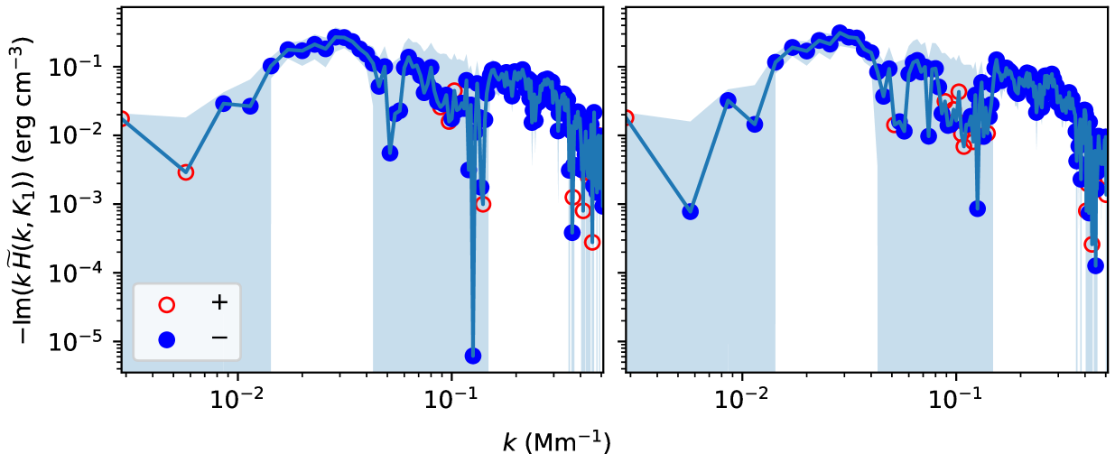
Figure 10: Magnetic helicity spectra calculated from different realizations of HMI magnetograms (in each case, the helicity spectra are averaged over Carrington rotations 2143--2153). Errors have been indicated by shaded regions of the same colour as the corresponding lines.

Recall that in HMI magnetograms (section 4.1.1), the sign of the transverse component of the magnetic field (i.e. the component normal to the line of sight) is chosen randomly in weak-field regions. One way to estimate the effect of this on the helicity spectra is to construct different realizations of each magnetogram by randomly flipping the sign of the transverse component at each position where the magnitude of the magnetic field is below 150G (the same threshold used to generate the HMI magnetograms).

Since each pixel in a synoptic magnetogram is computed by taking contributions from full-disk magnetograms where the corresponding pixels are close to the central meridian (Liu et al., 2017), it seems reasonable to assign to each pixel an effective line of sight that points in the direction $\left(\cos\lambda\right)\boldsymbol{\hat{r}}-\left(\sin\lambda\right)\boldsymbol{\hat{\lambda}}$. At each weak-field pixel, we then randomly flip the direction of the component transverse to the corresponding effective line of sight.

Figure 10 compares helicity spectra from two such realizations, showing that the changes in the helicity spectrum are consistent with the error estimated using equation 9.

References

- Astropy Collaboration et al. (2013) Astropy Collaboration, Robitaille, T. P., Tollerud, E. J., et al. 2013, A&A, 558, A33, doi: 10.1051/0004-6361/201322068
- Astropy Collaboration et al. (2018) Astropy Collaboration, Price-Whelan, A. M., Sipőcz, B. M., et al. 2018, AJ, 156, 123, doi: 10.3847/1538-3881/aabc4f
- Astropy Collaboration et al. (2022) Astropy Collaboration, Price-Whelan, A. M., Lim, P. L., et al. 2022, apj, 935, 167, doi: 10.3847/1538-4357/ac7c74
- Borrero et al. (2014) Borrero, J. M., Lites, B. W., Lagg, A., Rezaei, R., & Rempel, M. 2014, A&A, 572, A54, doi: 10.1051/0004-6361/201424584
- Brandenburg (2001) Brandenburg, A. 2001, ApJ, 550, 824–840, doi: 10.1086/319783
- Brandenburg et al. (2003) Brandenburg, A., Blackman, E., & Sarson, G. 2003, Advances in Space Research, 32, 1835–1844, doi: 10.1016/S0273-1177(03)90617-X
- Brandenburg et al. (2017) Brandenburg, A., Petrie, G. J. D., & Singh, N. K. 2017, The Astrophysical Journal, 836, 21, doi: 10.3847/1538-4357/836/1/21
- Brandenburg & Subramanian (2005) Brandenburg, A., & Subramanian, K. 2005, Physics Reports, 417, 1–209, doi: 10.1016/j.physrep.2005.06.005
- Charbonneau (2020) Charbonneau, P. 2020, Living Reviews in Solar Physics, 17, 4, doi: 10.1007/s41116-020-00025-6
- Dobler et al. (2006) Dobler, W., Stix, M., & Brandenburg, A. 2006, ApJ, 638, 336–347, doi: 10.1086/498634
- Elmore et al. (1992) Elmore, D. F., Lites, B. W., Tomczyk, S., et al. 1992, in Society of Photo-Optical Instrumentation Engineers (SPIE) Conference Series, Vol. 1746, Polarization Analysis and Measurement, ed. D. H. Goldstein & R. A. Chipman, 22–33, doi: 10.1117/12.138795
- Faurobert et al. (2009) Faurobert, M., Aime, C., Périni, C., et al. 2009, A&A, 507, L29–L32, doi: 10.1051/0004-6361/200913330
- Fleck et al. (2011) Fleck, B., Couvidat, S., & Straus, T. 2011, Sol. Phys., 271, 27–40, doi: 10.1007/s11207-011-9783-9
- Glogowski et al. (2019) Glogowski, K., Bobra, M. G., Choudhary, N., Amezcua, A. B., & Mumford, S. J. 2019, Journal of Open Source Software, 4, 1614, doi: 10.21105/joss.01614
- Gosain & Brandenburg (2019) Gosain, S., & Brandenburg, A. 2019, ApJ, 882, 80, doi: 10.3847/1538-4357/ab32ef
- Gosain et al. (2013) Gosain, S., Pevtsov, A. A., Rudenko, G. V., & Anfinogentov, S. A. 2013, ApJ, 772, 52, doi: 10.1088/0004-637X/772/1/52
- Grec et al. (2010) Grec, C., Uitenbroek, H., Faurobert, M., & Aime, C. 2010, A&A, 514, A91, doi: 10.1051/0004-6361/200811455
- Harker (2017) Harker, B. J. 2017, VFISV Inversion Code Documentation for SOLIS/VSM Pipeline Implementation, Tech. Rep. NSO/NISP-2017-02. https://arxiv.org/abs/1707.00002
- Harris et al. (2020) Harris, C. R., Millman, K. J., van der Walt, S. J., et al. 2020, Nature, 585, 357–362, doi: 10.1038/s41586-020-2649-2
- Hathaway (2015) Hathaway, D. H. 2015, Living Reviews in Solar Physics, 12, 4, doi: 10.1007/lrsp-2015-4
- Haugen et al. (2004) Haugen, N. E. L., Brandenburg, A., & Mee, A. J. 2004, Monthly Notices of the Royal Astronomical Society, 353, 947–952, doi: 10.1111/j.1365-2966.2004.08127.x
- Holzreuter & Solanki (2012) Holzreuter, R., & Solanki, S. 2012, A&A, 547, A46, doi: 10.1051/0004-6361/201219477
- Hunter (2007) Hunter, J. D. 2007, Computing in Science & Engineering, 9, 90–95, doi: 10.1109/MCSE.2007.55
- Keller et al. (2003) Keller, C. U., Harvey, J. W., & Giampapa, M. S. 2003, in Innovative Telescopes and Instrumentation for Solar Astrophysics, ed. S. L. Keil & S. V. Avakyan, Vol. 4853, International Society for Optics and Photonics (SPIE), 194 – 204, doi: 10.1117/12.460373
- Kishore & Singh (2025) Kishore, G., & Singh, N. K. 2025, The spectra of solar magnetic energy and helicity: scripts and simulation inputs, doi: 10.5281/zenodo.14958154
- Lesieur (2008) Lesieur, M. 2008, Fluid Mechanics and its Applications, Vol. 84, Turbulence in Fluids, 4th edn. (Springer)
- Liu et al. (2017) Liu, Y., Hoeksema, J. T., Sun, X., & Hayashi, K. 2017, Sol. Phys., 292, 29, doi: 10.1007/s11207-017-1056-9
- Luo et al. (2023) Luo, Y., Jiang, J., & Wang, R. 2023, The Astrophysical Journal, 954, 199, doi: 10.3847/1538-4357/acec77
- Moffatt (1978) Moffatt, H. K. 1978, Magnetic Field Generation In Electrically Conducting Fluids, Cambridge monographs on mechanics and applied mathematics (Cambridge University Press)
- Norton et al. (2006) Norton, A. A., Graham, J. P., Ulrich, R. K., et al. 2006, Sol. Phys., 239, 69–91, doi: 10.1007/s11207-006-0279-y
- Pariat et al. (2015) Pariat, E., Valori, G., Démoulin, P., & Dalmasse, K. 2015, A&A, 580, A128, doi: 10.1051/0004-6361/201525811
- Pencil Code Collaboration et al. (2021) Pencil Code Collaboration, Brandenburg, A., Johansen, A., et al. 2021, The Journal of Open Source Software, 6, 2807, doi: 10.21105/joss.02807
- Pipin & Pevtsov (2014) Pipin, V. V., & Pevtsov, A. A. 2014, ApJ, 789, 21, doi: 10.1088/0004-637X/789/1/21
- Pipin et al. (2019) Pipin, V. V., Pevtsov, A. A., Liu, Y., & Kosovichev, A. G. 2019, The Astrophysical Journal Letters, 877, L36, doi: 10.3847/2041-8213/ab21bf
- Pipin et al. (2013) Pipin, V. V., Zhang, H., Sokoloff, D. D., Kuzanyan, K. M., & Gao, Y. 2013, MNRAS, 435, 2581–2588, doi: 10.1093/mnras/stt1465
- Prabhu et al. (2021) Prabhu, A., Singh, N., Käpylä, M. J., & Lagg, A. 2021, A&A, 654, A3, doi: 10.1051/0004-6361/202141101
- Riley et al. (2014) Riley, P., Ben-Nun, M., Linker, J. A., et al. 2014, Sol. Phys., 289, 769–792, doi: 10.1007/s11207-013-0353-1
- Roberts & Stix (1971) Roberts, P., & Stix, M. 1971, The Turbulent Dynamo: A Translation of a Series of Papers by F. Krause, K.-H Radler, and M. Steenbeck, Tech. rep., doi: 10.5065/D6DJ5CK7
- Rudenko & Anfinogentov (2014) Rudenko, G. V., & Anfinogentov, S. A. 2014, Sol. Phys., 289, 1499–1516, doi: 10.1007/s11207-013-0437-y
- Seehafer (1990) Seehafer, N. 1990, Sol. Phys., 125, 219–232, doi: 10.1007/BF00158402
- Singh et al. (2018) Singh, N. K., Käpylä, M. J., Brandenburg, A., et al. 2018, The Astrophysical Journal, 863, 182, doi: 10.3847/1538-4357/aad0f2
- Virtanen et al. (2020) Virtanen, P., Gommers, R., Oliphant, T. E., et al. 2020, Nature Methods, 17, 261–272, doi: 10.1038/s41592-019-0686-2
- Zhang et al. (2014) Zhang, H., Brandenburg, A., & Sokoloff, D. D. 2014, The Astrophysical Journal Letters, 784, L45, doi: 10.1088/2041-8205/784/2/L45
- Zhang et al. (2010) Zhang, H., Sakurai, T., Pevtsov, A., et al. 2010, MNRAS, 402, L30–L33, doi: 10.1111/j.1745-3933.2009.00793.x
- Zhang (2006) Zhang, M. 2006, ApJ, 646, L85–L88, doi: 10.1086/506560