A Production Routing Problem with Mobile Inventories

Abstract

Hydrogen is an energy vector, and one possible way to reduce CO₂ emissions. This paper focuses on a hydrogen transport problem where mobile storage units are moved by trucks between sources to be refilled and destinations to meet demands, involving swap operations upon arrival. This contrasts with existing literature where inventories remain stationary. The objective is to optimize daily routing and refilling schedules of the mobile storages. We model the problem as a flow problem on a time-expanded graph, where each node of the graph is indexed by a time-interval and a location and then, we give an equivalent Mixed Integer Linear Programming (MILP) formulation of the problem. For small to medium-sized instances, this formulation can be efficiently solved using standard MILP solvers. However, for larger instances, the computational complexity increases significantly due to the highly combinatorial nature of the refilling process at the sources. To address this challenge, we propose a two-step heuristic that enhances solution quality while providing good lower bounds. Computational experiments demonstrate the effectiveness of the proposed approach. When executed over the large-sized instances of the problem, the median (resp. the mean) obtained by this two-step heuristic outperforms the median (resp. the mean) obtained by the direct use of the MILP solver by 12.7 $\mathrm{\%}$ (resp. 9 $\mathrm{\%}$), while also producing tighter lower bounds. These results validate the efficiency of the method for optimizing hydrogen transport systems with mobile storages and swap operations.

Keywords Production routing problem  $\cdot$ Hydrogen mobile storage  $\cdot$ Mixed-Integer Linear Program

1 Introduction

The global shift towards sustainable energy solutions has underscored the importance of hydrogen as a key component in reducing CO₂ emissions and addressing climate change concerns. Hydrogen not only offers a clean alternative fuel source, but also enhances energy security and flexibility. To support the expanding hydrogen economy, efficient transportation and distribution systems are essential for meeting (mobility) demands while minimizing operational costs.

In this paper, we address an optimal transport problem in which trucks are used to transport mobile hydrogen storage units (tanks) between sources and destinations. The sources represent supply locations where the storages are refilled with hydrogen, while the destinations correspond to sites where the stored hydrogen is consumed to meet mobility demands. The transport process operates bidirectionally, as storages are transported from sources to destinations to satisfy the demand and storages are also transported back from destinations to sources for refilling, ensuring a continuous supply cycle. Within a specified planning horizon, the transport problem objective is to find daily routing and refilling schedules of mobile storage units, in order to minimize an intertemporal cost taking into account transport, hydrogen purchase and demand dissatisfaction costs.

This work focuses on a variant of the Production Routing Problem (PRP), where mobile storages are moved by trucks between sources and destinations. Unlike conventional routing problems that assume static inventories [IRP_transshipment, IRP_pickup_delivery] at delivery locations, we use the concept of mobile inventories, allowing for dynamic relocation and swap operations upon delivery which are specific to hydrogen transport. This added layer of complexity requires optimizing daily routing and refilling schedules for mobile storage units.

Another distinguishing feature of this work, compared to the PRP found in the literature, is the highly combinatorial nature of the refilling process at the sources. This complexity arises from three factors: the constraint that exactly one storage unit must be present at each destination at any given time to satisfy demand, the constraint on the refilling capacity at the sources, and the fact that the stock of mobile storage units at the sources cannot be mixed. Specifically, when a new storage unit arrives from a source to replace the one previously stationed at the destination, the departing storage may not be empty, as it must be replaced immediately upon the arrival of the new mobile storage. As a result, multiple partially filled storage units may return to the same source, these units may also depart the next day without reaching full capacity because of refilling capacity at the sources. This, combined with the restriction on stock mixing, increases the complexity of the refilling process, as discussed later in §LABEL:constraints_node_source_1.

Now, we describe some assumptions that we make on the movements of storage units. When a storage unit is transported by truck from a source location to a destination location, an operation we refer to as a swap upon arrival is to be performed at destination: the truck exchanges the storage unit it carries with a storage unit located at the destination. Then, the newly positioned storage unit serves to meet demand at destination, while the collected storage returns to a source for refilling, transported by the same truck. To simplify the problem, we assume that the trip initialized by a truck on a specific day is completed within the same day. Moreover, we assume that, at initial time, there is a single storage unit at each destination. Then, during the optimization time span, we always have a single storage unit to meet demand at each destination (see Fig. 1).

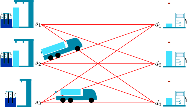
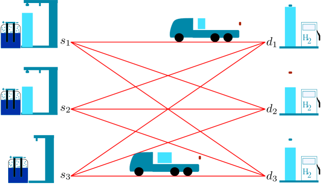
Figure 1: Storage unit delivery (left) and back to source after swap (right)

Moreover, we assume that each destination can receive at most one storage per day, that is, there is at most one swap per destination and per day. Using the previous assumptions, the delivery planning of storage units is done on a daily basis. Firstly, we need to determine what happens to the storage units at the source locations: whether they stay where they are or they be delivered to a destination. Second, we decide which source location the collected storage unit goes to.

Daily refill planning of the storage units involves determining the quantity of hydrogen to be purchased per source location per day. The daily maximum quantity of hydrogen purchased is assumed to be bounded. Moreover, when several storage units are present at a given source, the allocation of the purchased hydrogen between the present storage units is to be decided.

The rest of the paper is organized as follows. We review the existing literature in this field in Sect. 2. Afterwards, in Sect. 3, we give the notations and assumptions for our problem. We introduce the problem on a time-expanded graph in Sect. 4, and give its model in Sect. LABEL:sec:modeling. In Sect. LABEL:se:formulation_solving, we give the problem formulation and describe in detail the different algorithms. Numerical experiments are presented in Sect. LABEL:se:results. In Sect. LABEL:sec:flow_to_planning, we demonstrate how the storage routes (transport planning) can be derived from a solution of the problem on this time-expanded flow graph and finally the conclusion and possible directions for future works are discussed in Sect. LABEL:se:conclusion.

2 Literature review

Logistics and transport optimization have long been critical areas of research, with the Vehicle Routing Problem (VRP) (see for example [VRP2, VRP3, VRP1]) serving as a foundational framework for optimizing the delivery of goods and services. Extending the VRP, the Inventory Routing Problem (IRP) [thirty_years_IRP] integrates inventory management with routing decisions, while the Production Routing Problem (PRP) [PRP_review] further incorporates production planning.

As a generalization of the VRP, the IRP and PRP share its classification as an NP-hard problem [VRP_NP_HARD] which means that there is no known algorithm that can solve the IRP and PRP efficiently (in polynomial time).

Moreover, aside from the classical IRP and PRP, a wide range of variants have been studied in the literature. As an example, the IRP with transshipment [IRP_transshipment] and PRP with transshipment [PRP_transshipment] enable the transfer of goods between delivery locations, offering greater flexibility but introducing additional decision variables, whereas the IRP with pickup and delivery [IRP_pickup_delivery] and PRP with pickup and delivery [PRP_pickup_delivery] allow vehicles to visit pickup locations during their routes. These pickups can either be used for future deliveries or stored at the depot after completing the route. In [real_life_IRP], the authors propose a randomized local search algorithm to address large-scale instances of the IRP, that incorporates practical constraints such as time windows, driver safety, and site accessibility for vehicle resources. Additionally, they introduce a surrogate objective that ensures that short-term optimization solutions yield favorable long-term outcomes.

Several studies have examined real-life routing problems within the gas and hydrogen sectors [IRP_GAS3, IRP_GAS2, IRP_GAS1, ADMM, PRP_GAS1]. In [IRP_GAS3], a model for the liquefied natural gas sector is explored, introducing a decomposition algorithm using a path flow model with pre-generated duties and added valid inequalities. In [IRP_GAS2], the Stochastic Cyclic Inventory Routing Problem is addressed with supply uncertainty, applied to green hydrogen distribution in the Northern Netherlands. The study proposes a combined approach using a parameterized Mixed Integer Programming model for static, periodic vehicle transportation schedules and a Markov Decision Process to optimize dynamic purchase decisions under stochastic supply and demand. In [PRP_GAS1], the authors study a green PRP for medical nitrous oxide (N₂O) supply chains, integrating cost minimization and GHG emission reduction. A bi-objective model with a Branch-and-Cut algorithm and Fuzzy Goal Programming is developed to optimize production, transportation, and environmental impact. In [ADMM], the authors develop an optimization model for the integrated operation of an Electric Power and Hydrogen Energy System (IPHS), combining unit commitment, hydrogen production, transportation, and refueling. They formulate hydrogen transportation as a Vehicle Routing Problem (VRP) to optimize delivery routes. The overall problem is solved using an Augmented Lagrangian Decomposition method by dualizing the constraints linking the hydrogen production and transportation models. In [IRP_GAS1], a MILP model is developed for optimizing distribution and inventory in industrial gas supply chains, integrating vehicle routing with tank sizing to minimize costs. However, all these works typically assume fixed inventories.

In contrast, in this paper we focus on a novel variant of the PRP involving mobile inventories. This problem arises in the context of hydrogen distribution, where mobile storage units at destinations must be swapped and transported to other locations. To the best of our knowledge, studying this type of PRP, especially in the context of hydrogen transport, is new.

More precisely, the contributions of this paper are the following.

• We tackle a case study from an industrial partner about a hydrogen delivery problem.

• We introduce a new class of problems that we call Production Routing Problem with Mobile Inventories (PRP-MI). As already mentioned, PRP-MI are characterized by the fact that mobile storages at destinations can be swapped and transported to other locations. Additionally, since these mobile storages can arrive partially filled and depart without reaching full capacity, the refilling process at the sources presents a combinatorial challenge that must be taken into account in the model. In our study, these mobile storages are used for hydrogen distribution, however, the proposed framework can be applied to other transport problems with other commodities and similar logistical challenges.

• We propose a formulation of a PRP-MI optimization problem on a time-expanded graph and present an equivalent Mixed Integer Linear Program (MILP) model.

• We propose a two-step heuristic approach to effectively solve large-scale instances of the PRP-MI. First, this heuristic simplifies the problem by omitting the combinatorial constraints of the refilling process at the sources to obtain a transport plan for the storages. Second, it optimizes the quantities purchased at the sources and their allocation to the storages.

• We conduct comprehensive numerical experiments to compare the performance of three different methods for solving the PRP-MI, evaluating their solution quality across diverse problem instances.

3 Problem notations and assumptions

In this section, we turn the problem narrative given in the introduction to a more formal optimization problem description, and give all assumptions of the problem.

For that purpose, we start by introducing some notations. We denote by $\mathbb{J}=\{{1,\ldots,J}\}$ the set of days of the optimization planning horizon. Moreover, to follow the problem narrative and as suggested in Fig. 1, we need to refer to the time-intervals before and after a swap at each destination. For that purpose we introduce two sets related to day specification, the set $\underline{\mathbb{J}}=\{{\underline{j}\,|\,j\in\mathbb{J}}\}$ (resp. the set $\overline{\mathbb{J}}=\{{\overline{j}\,|\,j\in\mathbb{J}}\}$), where for a day $j$, the notation $\underline{j}$ stands for the first part of the day, when decisions to move storages from sources are made (resp. $\overline{j}$ stands for the second part of the day, when deciding to which source to return a storage unit after a swap at destination). We then consider the set $\widehat{\mathbb{J}}=(\underline{\mathbb{J}}\cup\overline{\mathbb{J}})\cup\{\overline{0}\}$ which is equipped with a finite total order:

$$\overline{0}\preceq\underline{1}\preceq\overline{1}\preceq\cdots\preceq\underline{J}\preceq\overline{J}\;,$$ (1)

and where $\overline{0}$ is an extra time index at which the initial conditions of the problem are given (see Figure LABEL:fig:example_expanded_graph). For $i\in\widehat{\mathbb{J}}$, we denote by $i^{+}$ the successor (resp. by $i^{-}$ the predecessor) of time $i$ if it exists in the total order $(\widehat{\mathbb{J}},\preceq)$:

$$\forall j\in\mathbb{J}\;,\enspace({\underline{j}})^{+} =\overline{j}\;,\enspace({\underline{j}})^{-}=\overline{j{-}1}\;,$$

$$\forall j\in\mathbb{J}\backslash\{{J}\}\;,\enspace({\overline{j}})^{+} =\underline{j{+}1}\;,\enspace$$

$$\forall j\in\mathbb{J}\;,\enspace({\overline{j}})^{-} =\underline{j}\;.$$

The hours within a day are denoted by $\mathbb{H}=\{{0,\ldots,23}\}$ and we denote by $\underline{h}=0$ the smallest (resp. $\overline{h}=23$ the greatest) element of $\mathbb{H}$.

We also denote by $\mathbb{S}$ the set of sources, by $\mathbb{D}$ the set of destinations (also called stations), and by $\mathbb{B}$ the set of mobile storage units. We denote by ${\cal G}=({\cal V},\mathcal{E})$ the undirected transportation graph. The set of nodes ${\cal V}$ is the disjoint union of the sources and destinations, that is ${\cal V}=\mathbb{S}\sqcup\mathbb{D}$. As we assume that there is no transport between two destinations or two sources, the graph ${\cal G}$ is a bipartite graph with respect to $\mathbb{S}$ and $\mathbb{D}$. Without loss of generality, the graph ${\cal G}$ is assumed to be complete, meaning that each destination is reachable from any source and vice-versa with known transport times that are not necessarily symmetric. Specifically, the transport time from a source $s$ to a destination $d$, denoted as $t_{s,d}$, may differ from the transport time from the same destination $d$ back to the same source $s$, denoted as $t_{d,s}$. In addition to the transport time between a source and a destination, we consider a mapping $g:\mathbb{S}\times\mathbb{D}\to{\mathbb{R}}_{+}$ which for a given oriented pair $(s,d)$, $g(s,d)$ gives the sum of three terms: the time needed to load the truck with a storage unit at the source $s$; the transport time from $s$ to $d$; the swap time of the storage units at the destination $d$.

For any set $\mathbb{A}$, we denote by $\mathbf{1}_{\mathbb{A}}(\cdot)$ the indicator function of $\mathbb{A}$ that equals $1$ when its argument belongs to $\mathbb{A}$ and $0$ otherwise, by $\Delta_{\mathbb{A}}$ the diagonal set $\Delta_{\mathbb{A}}=\{{(a,a)\,|\,a\in\mathbb{A}}\}\subset A^{2}$ and, when $\mathbb{A}$ is finite, by ${\lvert\mathbb{A}\rvert}$ its cardinality. Finally, for all $n\in{\mathbb{N}}$, where ${\mathbb{N}}$ is the set of natural numbers, we denote the set $\{{1,\ldots,n}\}$ by $[n]$.

The following assumptions are made on the transport model:

1. : All mobile storage units have the same maximal capacity, denoted by $\overline{S}$;

2. : The maximal capacity $\overline{S}$ is designed to meet at least one day’s demand at any destination;

3. : Each destination can receive at most one storage per day;

4. : Each storage is transported at most once per day;

5. : Each truck departing from a source $s\in\mathbb{S}$ starts at a given predetermined hour in the morning $h_{0}$;

6. : The maximum number of storage units that can stay at source $s\in\mathbb{S}$ is bounded by $\kappa(s)\in{\mathbb{N}}$;

7. : There is no refill at the sources during the first part of the day;

8. : There is always exactly one storage per destination per day (except during a swap).

As introduced previously, we have two time scales in the transport problem, a day time scale ($\mathbb{J}$) and an hour time scale ($\mathbb{H}$). We have introduced a day split in two parts in the previously and we give now the consequence of this day split at hour level. Given a source $s$ from which a storage unit is sent to a destination $d$, the end of the swap at destination will occur at hour $h_{0}+g(s,d)$ using Assumption $A_{4}$ and $A_{5}$ and the definition of the mapping $g$. At each destination $d\in\mathbb{D}$, we divide each day $j$ duration into two time periods: the first part of the day which is the time period $[\underline{h},h^{\textsf{sw}}_{s,d,j}[$ from midnight ($\underline{h}$) to $h^{\textsf{sw}}_{s,d,j}$, where $h^{\textsf{sw}}_{s,d,j}$ denotes the hour at which the swap ends at destination $d$ at day $j$ and the last, or second, part of the day which is the time period $[h^{\textsf{sw}}_{s,d,j},\overline{h}+1[$ from the end of swap until midnight ($\overline{h}+1$). Indeed, using the definition of the function $g$ and of time $h_{0}$, we have that $h^{\textsf{sw}}_{s,d,j}=h_{0}+g(s,d)$, where $s$ is the source from which the storage unit was transported to $d$ on day $j$. Together with Assumption $A_{3}$, during a fixed day, we obtain that at most two distinct storages are used to fulfill the demand, one for each time period. Finally, if during day $j$ no storage is sent to destination $d$, there is no swap time at destination and we arbitrarily divide the day into two time periods, which will be explained in more details later in Equation (LABEL:eq:forced_swap_time). An example of a swap is illustrated in Fig. 2.

$$s\to\overbrace{\includegraphics[scale={.15}]{truckr}}^{\text{from $s$ to $d$}}\to d\hskip 56.9055pt\underbrace{\includegraphics[scale={0.15}]{truckVr}}_{\text{swap at $d$}} \hskip 56.9055ptd\to\overbrace{\includegraphics[scale={0.15}]{truckb}}^{\text{from $d$ to $s^{\prime}$}}\to s^{\prime}$$

$$\underbrace{\mbox{\includegraphics[height=42.67912pt]{dest_lj}}\hskip 42.67912pt}_{\text{$d$: first part of the day $[0,h^{\textsf{sw}}_{s,d,j}[$}} \underbrace{\mbox{\includegraphics[height=42.67912pt]{dest_rj}}}_{\text{$d$: second part of the day $[h^{\textsf{sw}}_{s,d,j},\overline{h}[$}}$$

Figure 2: The day division at a destination $d$: a truck picks up a storage unit from the source $s$ at $h_{0}$, transports it to the destination $d$, performs the swap, and then returns the collected storage unit back to a source $s^{\prime}$. During the first part of the day, the (blue) mobile storage originally located at destination $d$ satisfies the demand, and during the second part of the day, the newly arrived mobile storage (red) fulfills the demand

4 Problem description on a time-expanded flow graph

In the context of routing problems with a fleet of vehicles, previous studies (e.g., [comparison_formulation_IRP1, comparison_formulation_IRP2]) have demonstrated that vehicle-indexed formulations yield high-quality solutions when considering complete tours and a limited number of vehicles (typically fewer than five). However, our problem differs in that the routes follow a back-and-forth structure: storage units depart from the source, reach a destination, and the storage unit previously stationed at that destination immediately returns, rather than forming complete multi-stop tours.

Moreover, in our case, it is the mobile storage units that are transported between locations and that require the monitoring of their stock, making a storage-indexed formulation more appropriate rather than a vehicle-indexed formulation. This approach, however, poses a significant numerical challenge as we expect our model to handle a large number of storage units, and using a storage-indexed formulation leads to an excessive number of variables. In a preliminary study (not described here), we experimented with such formulation but encountered severe computational difficulties due to the presence of symmetrical solutions. For example, if two identical full storage units are available at a source for dispatch, interchanging them does not alter the solution structure or cost, yet it introduces redundancies that significantly impact solver performance. This issue is further exacerbated as the number of mobile storage units increases, and in the absence of appropriate symmetry-breaking constraints. We refer to the study in [Margot2010] for the analysis of MILP models in the presence of symmetries.

To keep the number of variables reasonable and to avoid such symmetries, we propose a time-expanded graph reformulation of our problem. This reformulation eliminates the need for mobile storage indexing, thereby breaking some symmetries and is expected to improve numerical resolution. For that purpose, we build from the transport graph a new graph commonly called [time_expended_network, time_expended_network2] a time-expanded graph (or graph dynamic network flow). The transport of storage unit is replaced by considering both continuous and binary flow variables attached to the arcs of the time-expanded graph and satisfying flow conservation equations (Kirchhoff law) at the graph nodes (to be explained later).

In Sect. LABEL:sec:flow_to_planning, we demonstrate how the storage routes (transport planning) can be derived from a solution of the problem on this time-expanded flow graph.

4.1 Definition of the time-expanded graph

We turn now to the precise description of the time-expanded graph. In §4.1.1 we define the nodes of the time-expanded graph and in §4.1.2, we define its arcs.

4.1.1 Definition of nodes

First, we define the set of nodes of the time-expanded graph. Each node of the expanded graph is an ordered pair composed of a node of the physical transportation graph (source or destination), that is an element of ${\cal V}$, and of a time index belonging to $\widehat{\mathbb{J}}=\underline{\mathbb{J}}\cup\overline{\mathbb{J}}\cup\{\overline{0}\}$. Thus, the set of nodes of the time-expanded graph, denoted as ${\cal V}^{\textsf{te}}$, is defined by ${\cal V}^{\textsf{te}}={\cal V}\times\widehat{\mathbb{J}}$.

4.1.2 Definition of arcs

Second, we define the arcs of the time-expanded graph. The time-expanded graph we build is an oriented multigraph, that is, each edge in the graph is oriented, and two nodes may be connected by more than one oriented edge. As it is used to model physical flows between nodes, an arc is only present between two nodes of ${\cal V}^{\textsf{te}}$ indexed by two consecutive elements of the time index $\widehat{\mathbb{J}}$, that is, between a node $(v,i)$ and a node $(v^{\prime},i^{+})$ where $i^{+}$ is the successor of $i\in\widehat{\mathbb{J}}$ (see Equation (1)). For that reason, we only use one time index in an arc specification, that is, the arc $(v,i)\mapsto(v^{\prime},i^{+})$ in the time-expanded graph is denoted by $(v,v^{\prime},i)$ and $\varphi_{v,v^{\prime},i}$ when an arc is used as a flow index and a specific notation when two nodes are connected by several arcs as described now.

Since at most one storage unit is transported between a source and a destination (and vice-versa) using Assumption $A_{3}$, and exactly one storage is present at each destination and each time using Assumption $A_{8}$, a single arc $(v,v^{\prime},i)=(v,i)\mapsto(v^{\prime},i^{+})$ is sufficient to represent the flow of hydrogen between two nodes $(v,i)$ and $(v^{\prime},i^{+})$ of the time-expanded graph for $(v,v^{\prime})\in(\mathbb{S}{\times}\mathbb{D})\cup\Delta_{\mathbb{D}}$ or $(v,v^{\prime})\in(\mathbb{D}{\times}\mathbb{S})\cup\Delta_{\mathbb{D}}$, where $\mathbb{S}\times\mathbb{D}$ and $\mathbb{D}\times\mathbb{S}$ correspond to the arcs of the physical graph ${\cal G}$, and, the addition of $\Delta_{\mathbb{D}}$ ensures that a storage located at a destination can remain at that destination, while also preventing its transport to a different destination. However, the situation is slightly more complicated when the two involved physical nodes are the same source node, that is $v=v^{\prime}$ with $v\in\mathbb{S}$. As multiple storage units may remain at a source without being dispatched to a destination, we need several arcs between $(s,i)$ and $(s,i^{+})$ for $s\in\mathbb{S}$. This number of arcs is bounded for each source $s\in\mathbb{S}$ by the value $\kappa(s)$ where the function $\kappa$ is given by Assumption $A_{6}$. Finally, for $k\in[\kappa(s)]$, the notation