Loop vs. Bernoulli percolation on trees:
strict inequality of critical values

Abstract

We consider loop ensembles on random trees. The loops are induced by a Poisson process of links sampled on the underlying tree interpreted as a metric graph. We allow two types of links, crosses and double bars. The crosses-only case corresponds to the random-interchange process, the inclusion of double bars is motivated by representations of models arising in mathematical physics. For a large class of random trees, including all Galton-Watson trees with mean offspring number in $(1,\infty)$, we show that the threshold Poisson intensity at which an infinite loop arises is strictly larger than the corresponding quantity for percolation of the untyped links. The latter model is equivalent to i.i.d. Bernoulli bond percolation. An important ingredient in our argument is a sensitivity result for the bond percolation threshold under downward perturbation of the underlying tree by a general finite range percolation. We also provide a partial converse to the strict-inequality result in the case of Galton-Watson trees and improve previously established criteria for the existence of an infinite loop in the case were the Galton-Watson tree has Poisson offspring.

AMS-MSC 2020: 60K35, 82B26, 82B31

Key Words: percolation, phase transition, random interchange, random loop model, random stirring

1 Introduction

Recent years have seen increasing interest in the cycle and permutation structure of the random stirring model that was introduced by Harris [15] in the early 1970s. Also known as the random-interchange process, this model has attracted attention for its connection to the quantum Heisenberg model. It is also valued as a beautiful probabilistic method for studying permutations with geometric constraints.

On a graph $G=(V,E)$, the random interchange process is defined as follows: Each node of the graph initially hosts a labelled particle, and each edge of the graph is equipped with an independent Poisson process of rate $\beta>0$. Whenever the Poisson clock associated with an edge rings, the two particles at the endpoints of that edge swap positions. This process induces a random permutation $\pi_{\beta}:V\to V$ for any $\beta>0$.

A long-standing conjecture of Tóth is that for $\mathbb{Z}^{d}$ with $d\geq 3$ and sufficiently large $\beta$, the permutation $\pi_{\beta}$ contains infinite cycles almost surely. A major step towards the resolution of Toth’s conjecture is the recent work of Elboim and Sly [11], who prove that infinite cycles exist almost surely for $d\geq 5$.

Observe that in order to obtain a cycle, it is necessary to have at least one Poisson point on each edge of the cycle. This observation leads to a necessary condition for the existence of infinite loops: there must be an infinite percolation cluster in the Bernoulli edge percolation with retention probability $1-e^{-\beta}$ induced by the Poisson process. The main question we investigate in the present article is whether this condition is also sufficient.

A remarkable result by Schramm [24] shows that on the complete graph $K_{n}$, where edge rates are $\beta/n$, the existence of infinite cycles and the emergence of an infinite percolation cluster are asymptotically equivalent as $n\to\infty$, implying that their critical parameters coincide. Moreover, it is shown that the normalised ordered sizes of the loops in the giant component exhibit a Poisson-Dirichlet $\operatorname{PD}(1)$ structure.

In contrast to Schramm’s result, Mühlbacher [22] showed that on infinite graphs of bounded degree, the two critical parameters differ. An explicit lower bound on the size of this difference was recently provided by Betz et al. [7].

Thus, whether percolation is also a sufficient condition depends on the underlying graph. Our main result extends the inequality of the critical values to certain sparse graphs of unbounded degree:

For a large class of transient infinite trees $T$ of finite Hausdorff dimension, the critical values for the random interchange process and the induced percolation are different.

We refer the reader to Theorem A for the rigorous formulation of the statement and, in particular, the precise description of which trees are covered.

In fact, our result is more general, as it extends to the random loop model. The random loop model was introduced as a representation of certain important quantum spin systems. The random stirring model gives a representation of the ferromagnetic Heisenberg model, where points of the Poisson process are referred to as crosses. This representation was introduced by Powers [23] and then used by Tóth [25] to give a lower bound on the pressure. There is also a representation of the anti-ferromagnetic Heisenberg model proposed by Aizenman and Nachtergaele [1]. This representation also involves independent Poisson point processes of intensity $\beta$ assigned to the edges of $G$. However, unlike the random stirring model, the points of these Poisson processes, referred to as bars, do not correspond to transpositions, and the resulting random structure is richer than a permutation.

Ueltschi [26] observed that these representations can be unified to describe XXZ-models. In this setting, the intensity of crosses is given by $u\beta$, while the intensity of bars is $(1-u)\beta$ for some $u\in[0,1]$. We collectively refer to crosses and bars as links. By following these links along $G\times[0,1)_{\text{per}}$, we uncover a set of loops $\mathcal{L}$; see Figure 1 for an illustration.

The connection to spin-$S$ quantum systems requires an exponential tilt of the loop distribution by $\theta^{\sharp\mathcal{L}}$ with $\theta=2S+1$. However, the model remains of interest even for the case $\theta=1$ which is the case we treat.

The central question in the study of the random loop model remains whether a phase transition occurs. This problem is particularly challenging to analyse due to the inherent dependencies in the model. Nonetheless, two extreme cases are well understood, namely regular trees and the complete graph.

On the one hand, for regular trees, Angel [3] established the existence of two distinct phases for $\theta=1$ on $d$-regular trees with $d\geq 4$ and showed that infinite cycles appear for $\beta\in(d^{-1}+\tfrac{13}{6}d^{-2},\log(3))$ when $d$ is sufficiently large. Hammond [13] later proved that for $d\geq 2$, there exists a critical value $\beta_{0}$ above which infinite cycles emerge in the case $u=1$, a result extended by Hammond and Hegde [14] to all $u\in[0,1]$. Björnberg and Ueltschi provided an asymptotic expression for the critical parameter for loops up to second order in $d^{-1}$ [9] and further extended this analysis to the case $\theta\neq 1$ [10]. A comprehensive picture for $d$-regular trees with $d\geq 3$, $\theta=1$, and $u\in[0,1]$ was established by Betz et al. in [6], proving a (locally) sharp phase transition for infinite loops in the interval $(0,d^{-1/2})$ and deriving explicit bounds on the critical parameter up to order 5 in $d^{-1}$.

Here, we mainly consider the loop model under quenched disorder, meaning that the underlying tree is itself random, which adds another layer of complexity to the problem. Betz et al. [5] studied the case where $T$ is drawn from a Galton-Watson distribution and established the existence of a phase transition under specific conditions on the offspring law. For Galton-Watson trees, we investigate sharpness of our criterion, i.e. whether the critical values coincide if the expected number of offspring (and therefore the Hausdorff dimension) is infinite. Indeed:

If the tail of the offspring distribution in a Galton-Watson tree is sufficiently heavy, then the critical values for the random interchange process and the induced percolation coincide.

The precise tail condition is given in Theorem B below, and Galton-Watson trees are discussed at length in Section 4.

We believe our results are indicative of the general behaviour of the critical values on trees:

Problem. For any $u\in[0,1]$ and any tree $T$, show that the critical values for loop percolation and link percolation are different if and only if the Hausdorff dimension of $T$ is finite and positive.

This conjectured behaviour on trees and Tóth’s conjecture for $\mathbb{Z}^{d}$ might incline one to believe that the critical value for loop percolation should be finite, whenever $T$ is transient. This is not the case, since there are transient trees with in which even bond percolation has no phase transition, as shown e.g. by Lyons [17].

Note that Schramm’s result [24] on the complete graph is expected to generalise to a large number of dense graphs. Björnberg et al. [8] showed the emergence of a $\operatorname{PD}(\tfrac{1}{2})$ structure on $K_{n}$ when $u\neq 1$. The agreement of the two critical parameters has also been established for the hypercube by Kotecký et al. [16] and for Hamming graphs by Miłoś and Şengül [21].

Thus, trees represent sparse graphs whose structure becomes denser as their dimension increases, interpolating smoothly between the bounded-degree setting and the diverging-degree asymptotic regimes studied in previous work.

Outline of the remaining sections.

In Section 2, we introduce the random loop model, define its critical parameters, and state our main results Theorem A and B. Section 3 discusses the couplings we use in the proof of Theorem A. In Section 4, we discuss in detail the case of Galton-Watson trees. Section 5 introduces potential theory on general trees and establishes auxiliary results for the proof of Theorem A, most importantly Theorem 5.3 which establishes sensitivity of the bond percolation threshold under finite range percolation processes. Finally, in Section 6, we prove Theorem A.

2 Model and main results

The random loop model is well-established and precisely defined in various papers, such as [26] and [6]. We restrict ourselves to a brief overview of the main objects. Let $G=(V,E)$ denote a simple, connected graph with vertex set $V$ and edge set $E\subset\{\{x,y\}:x,y\in V,x\sim y\}$. In this paper, we always think of $G$ as a rooted graph, i.e. a pair $(G,o)$ of a graph $G$ and a distinguished vertex $o\in V$ that we call the root.

The space underlying a configuration is $E\times[0,1)$, i.e. to each edge, we attach a copy of the interval $[0,1)$. Let $u\in[0,1]$. and $\beta>0$ be fixed. On $E\times[0,1)$, we define two independent homogeneous Poisson point processes: one with intensity $\beta u$ whose points we call crosses, and another with intensity $(1-u)\beta$ whose points we call (double) bars. We refer to crosses and double-bars collectively as links. The full configuration space is denoted by $\Omega(G)=\mathcal{N}^{E}\times\mathcal{N}^{E}$, where $\mathcal{N}$ is the space of simple counting measures on $\mathcal{B}[0,1]$, the Borel $\sigma$-field of the interval $[0,1)$. We denote the distribution of the graph $G$ edge-marked by the Poisson processes by $\rho_{G,\beta,u}$. When it is necessary to specify, we will denote by $I(e)$ the copy of $[0,1)$ attached to $e$. For a realization $\omega\in\Omega(G)$, we denote by $m_{e}=m_{e}(\omega)\in\mathbb{N}\cup\{0\}$ the number of links on $e$ and by $M=M(\Omega)\in\mathbb{N}\cup\{0,\infty\}$ the total number of links.

The crosses and double bars form loops, defined by the following rules:

• We start at a point $(x,t)\in V\times[0,1)$ and move in the positive time direction, thereby exploring links on edges adjacent to $x$.

• If we encounter a double bar at $(\{x,y\},\tau\pm)$, we jump to $(y,\tau\pm)$ and change time direction.

• If we encounter a cross at $(\{x,y\},\tau\pm)$, we jump to $(y,\tau\mp)$ and continue in the same time direction.

• If, for any vertex $z$, we reach $(z,1)$ whilst moving in the positive time direction then we jump to $(z,0)$ and continue moving in the positive time direction. If we reach $(z,0)$ whilst moving in the negative time direction then we jump to $(z,1)$ and continue moving in the negative time direction.

• If we reach $(x,t)$ again, the loop is complete.

We observe that loops are closed trajectories in the space $V\times[0,1)$. This concept is best understood with the aid of a visual illustration such as in Figure 1. Notice that the last rule means that we treat time as cyclic, in particular, we may interpret the $I(e),e\in E,$ as tori in one dimension.

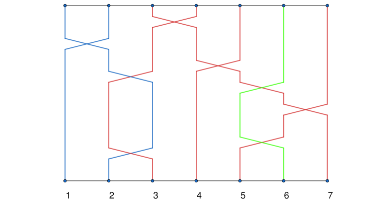
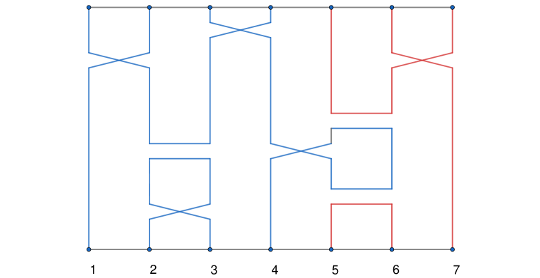
Figure 1: Example loop configurations. On the left is and example of the case $u=1$ of only crosses. On the right the case $u\in(0,1)$ so that crosses and bars are both present.

We denote the set of loops for a given configuration $\omega$ by $\mathcal{L}(\omega)$ and fix $\theta\in\mathbb{R}_{>0}$. The loop-weighted measure discussed in the introduction is defined by

$$\mathsf{loop}_{\beta,\theta}[G](\mathrm{d}\omega)\coloneqq\frac{1}{Z(G,\beta,u,\theta)}\,\theta^{\sharp\mathcal{L}(\omega)}\,\rho_{G,\beta,u}(\mathrm{d}\omega),$$

where $Z(G,\beta,u,\theta)$ denotes the partition function, defined as

$$Z(G,\beta,u,\theta)\coloneqq\int_{\Omega(G)}\theta^{\sharp\mathcal{L}(\omega)}\,\rho_{G,\beta,u}(\mathrm{d}\omega).$$

When $\theta\in\mathbb{N}$, this expression admits a natural interpretation: each loop is uniformly assigned one of $\theta$ distinct colours from the set $[\theta]=\{1,\dots,\theta\}$.

In this article, we will work in the case $\theta=1$. Therefore, we simplify the notation to $\mathsf{loop}_{\beta}[G]$.

Based on this framework, we define the concept of connection within the model. Two points $(x,t)$ and $(x^{\prime},t^{\prime})$ are said to be connected, denoted by $(x,t)\Leftrightarrow(x^{\prime},t^{\prime})$, if they are in the same loop. In particular, when considering the event that a point $(x,0)$ is connected to the origin $(o,0)$, we define this connection event as $o\Leftrightarrow x$. Note that these conventions define two distinct equivalence relations: one on $V\times[0,1)$ and one on $V$.

Let $L_{o}$ be the loop containing $(o,0)$. By $|L_{o}|,$ we denote the total length of the loop, i.e. the total Lebesgue measure of the time the loop spends in each of its vertices. Note that jumps along links are considered instantaneous and are only represented as taking up positive time in the Figure 1 for illustration purposes. Note that if $u=1$ and $|L_{o}|<\infty$ we have

$$|L_{o}|=\sharp\{x:o\Leftrightarrow x\},$$

i.e., the loop length corresponds precisely to the size of the permutation cycle induced by the crosses interpreted as transpositions of vertices along edges. We can define $L_{x}$ for other vertices $x\in V$ analogously. An infinite loop is a loop of infinite length. We denote the critical parameter for loop percolation on $G$ or loop percolation threshold of $G$ by

$$\beta^{\textup{loop}}_{c}(G)\coloneqq\inf\bigg{\{}\beta\geq 0:\mathsf{loop}_{\beta}[G]\big{(}|L_{o}|=\infty\big{)}>0\bigg{\}}.$$

Using connectedness of $G$, it is not difficult to see that this quantity is well-defined and does not depend on the choice of the vertex $o$, cf. [3]. Note that $\beta^{\textup{loop}}_{c}(G)$ in general depends on $u$.

The loop measure induces another natural percolation structure where we obtain a random subgraph of $G$ by retaining edges with probability $1-e^{-\beta}$. This corresponds to $\mathsf{loop}_{\beta}[G]\big{(}m_{e}\geq 1\big{)}$, recalling that $m_{e}$ denotes the number of links on $e\in E$. An edge is said to be retained if there exists at least one link on it and it is said to be removed otherwise. We denote the measure of this percolation model by $\mathsf{link}_{\beta}[G]$ and refer to the corresponding percolation process as link percolation.

We say that $x$ and $y$ are connected in the subgraph of $G$ obtained by $\mathsf{link}_{\beta}[G]$ if there exists a sequence of vertices $(v_{k})_{0\leq k\leq K}$ such that $v_{0}=x$, $v_{K}=y$, and $\{v_{k},v_{k+1}\}\in E$ is retained for every $0\leq k<K$. This event is denoted by $x\leftrightarrow y$. The connected component or cluster of a vertex $x\in V$ with respect to link percolation on $G$ is defined as $C_{x}\coloneqq\{v\in V:x\leftrightarrow v\}$.

Furthermore, we write $o\leftrightarrow\infty$ if the connected component of $o$ under $\mathsf{link}_{\beta}[G]$ is infinite or, equivalently, there exists an infinite self-avoiding path of retained edges starting at $o$. The critical parameter for the link percolation model is defined as

$$\beta^{\textup{link}}_{c}(G)\coloneqq\inf\big{\{}\beta\geq 0\,:\,\mathsf{link}_{\beta}[G]\big{(}o\leftrightarrow\infty\big{)}>0\big{\}}.$$

Unlike $\beta^{\textup{loop}}_{c}(G)$, $\beta^{\textup{link}}_{c}(G)$ never depends on $u$.

Remark 2.1.

Since $\rho_{G,\beta,u}$ is derived from an i.i.d. collection of Poisson processes, it follows from Kolmogorv’s $0$-$1$ law, that $\mathsf{link}_{\beta}[G]\big{(}o\leftrightarrow\infty\big{)}>0$ (or $\mathsf{loop}_{\beta}[G]\big{(}|L_{o}|=\infty\big{)}>0$, respectively) if and only if $\mathsf{link}_{\beta}[G]\big{(}\exists x\in V:x\leftrightarrow\infty\big{)}=1$ (or $\mathsf{loop}_{\beta}[G]\big{(}\exists x\in V:|L_{x}|=\infty\big{)}=1$, respectively). Thus we could equivalently have defined the critical value(s) using the latter expression(s).

We focus on random ensembles of trees that satisfy an ergodicity property which ensures that the critical values do not depend on the realisation. More precisely, we work with stationary trees in the sense of [4]. Let us briefly introduce the setup, for a more detailed discussion we refer the reader to [4, 20, 2]. A rooted graph $(G,o)$ is a graph with a distinguished root vertex $o$. An isomorphism between rooted graphs $(G,o_{G})$ and $(H,o_{g})$ is a bijective edge preserving map $i:V(G)\to V(H)$ with $i(o_{G})=o_{H}$. We consider rooted graphs equivalent, if there exists an isomorphism between them. Let $\mathscr{G}_{\ast}$ denote the set of all locally finite rooted graphs up to graph isomorphism. By a slight abuse of notation, we do not distinguish between graphs and their isomorphism classes. Define

$$\textup{d}_{\ast}\big{(}(G,o_{G}),(H,o_{H})\big{)}=\inf\Big{\{}\frac{1}{R+1}:B_{G}(o_{G},R)\text{ is rooted isomorphic to }B_{H}(o_{H},R)\Big{\}},$$

where $B_{G}(v,R)$ denotes the graph-distance-$R$ neighbourhood of $v$ in $G$ for any graph $G$, $v\in V(G)$, and $R\in\{0,1,\dots\}$. Together with the topology induced by $\textup{d}_{\ast}$, $\mathscr{G}_{\ast}$ is a Polish space. Consider a probability measure $\mu$ on $\mathscr{G}_{\ast}$. Given a realisation $(G,o)$ of $\mu$, the simple random walk $(S_{t},t\geq 0)$ on $G$ started at the root $S_{0}=o$ is well-defined due to local finiteness of $G$. We call $\mu$ invariant (with respect to simple random walk), if

$$(G,o)\overset{d}{=}(G,S_{1})$$

where $\overset{d}{=}$ indicates equality in distribution for random variables on $\mathscr{G}_{\ast}$. We interpret the map $(G,o)\mapsto(G,S_{1})$ as a shift on $\mathscr{G}_{\ast}$. Hence $\mu$ is invariant if and only if it is invariant with respect to shifts in the usual ergodic theoretic sense. In a similar vein, we can define a shift-invariant $\sigma$-field $\mathbb{I}$ containing those Borel-sets of $\mathscr{G}_{\ast}$ which are invariant under shifts. Intuitively, $\mathbb{I}$ contains those events that do not depend on a vicinity of the root. A random rooted graph $(G,o)\in\mathscr{G}_{\ast}$ is now called stationary if its distribution $\mu$ is invariant and it is called ergodic if the shift-invariant $\sigma$-field $\mathbb{I}$ is $\mu$-trivial. A random rooted tree corresponds to the case where $\mu$ is supported on the subspace $\mathscr{T}_{\ast}\subset\mathscr{G}_{\ast}$ of trees. It can be shown that, if $G$ is stationary and ergodic, one has

$$\lim_{n\to\infty}\frac{|S_{n}|}{n}=:s\in[0,1]\text{ almost surely and in }L_{1},$$ (1)

see e.g. [4, Theorem 2.2]. We call $s$ the speed of the simple random walk on $G$. We say that $G$ is ballistic if $s>0$.

We are now ready to provide a precise formulation of our main result. For any metric space $X$, let $\dim(X)$ denote its Hausdorff dimension and recall that the boundary $\partial T$ of a rooted tree $(T,o)$ is the metric space induced by infinite self-avoiding walks on $(T,o)$, see Section 5 for more detail.

Theorem A.

Fix $u\in[0,1]$. Let $(T,o)\in\mathscr{T}_{\ast}$ be a stationary, ergodic and ballistic tree with $\dim(\partial T)<\infty$. Then

$$\beta_{c}^{\mathsf{loop}}(T)>\beta_{c}^{\mathsf{link}}(T).$$

Theorem A is proved in Section 6, after we have introduced the notation and results needed for the proof.

As alluded to in the introduction, in the special case of Galton-Watson trees, we contrast Theorem A with a sufficient criterion for the coincidence of the critical values.

Theorem B.

Let $(T,o)$ denote a Galton-Watson tree with offspring law $\zeta$. Denote by $f=f_{\zeta}$ the probability generating function of $\zeta$. If there exists $\varepsilon_{0}>0$ such that

$$\sqrt{\varepsilon}f^{\prime}(1-\varepsilon)>\tfrac{1}{\sqrt{2}}\quad\text{ for all }\varepsilon\in(0,\varepsilon_{0}),$$ (2)

then $\beta_{c}^{\textup{loop}}=\beta_{c}^{\textup{link}}=0$.

The proof of Theorem B is not very difficult and is included in the proof of Theorem 4.1. The significance of Theorem B stems solely from the fact that it indicates that coincidence of the critical values arises precisely at the edge of the sparse regime, since the condition on the tail of $\zeta$ implicit in (2) in particular implies that $\dim(\partial T)=\infty$ conditionally on the survival of $T$.

We close this section with an example that demonstrates the intricate relation between $\beta_{c}^{\mathsf{loop}}(T)$ and the underlying tree $T$. In particular, our example indicates the difficulty of obtaining monotonicity results for loop percolation.

Example 2.2.

Consider the case where $T=(T_{d},o)$ is a rooted $d$-regular tree and consequently $\beta_{c}^{\mathsf{link}}(T)$ satisfies $1-\exp(-\beta_{c}^{\mathsf{link}}(T))=1/d$. By coupling the survival of the loop at $(o,0)$ to a Galton-Watson process is was shown [6, Equation (2.3)] that for $3\leq d\leq 100$

$$0\leq\beta_{c}^{\mathsf{loop}}(T)-\bigg{(}\frac{1}{d}+\frac{\tfrac{5}{6}-\tfrac{2}{3}u+\tfrac{5}{6}u^{2}}{d^{2}}+\frac{\tfrac{2}{3}-\tfrac{11}{10}u+\tfrac{91}{30}u^{2}-\tfrac{41}{10}u^{3}+\tfrac{29}{12}u^{4}}{d^{3}}\bigg{)}\leq\frac{2}{d^{4}}.$$

For simplicity, we will restrict ourselves to the case $u=1$. In this case there are only crosses and the effect of placing a link at $(\{x,y\},t)$ is to merge the loops at $(x,t)$ and $(y,t)$ if they are distinct, or to split the loop containing $(x,t)$ and $(y,t)$ into two loops, one containing $(x,t-)$ and $(y,t+)$, and the other containing $(x,t+)$ and $(y,t-)$.

Consider modifying $(T_{d},o)$ by adding $S$ leaves to every vertex of the graph, call this new graph $T(S)$. Note that $\beta_{c}^{\mathsf{link}}(T(S))$ does not depends on $S$. When exploring the loop from the root, a leaf $\ell$ with zero or one links to its parent does not affect the support of the loop on the underlying $d$-regular tree. However, a leaf $\ell$ with $k\geq 2$ links to its parent will take the loop to the leaf and return it to its parent after some time corresponding to the first order statistic of $k-1$ Uniform[0,1] random variables (a Beta$(1,k-1)$ random variable). If $S\gg d$ then on arriving at a vertex $x$ at time $t$ we will, before time $t+\varepsilon$, enter a leaf with $k\geq 2$ links to $x$ and then be returned to $x$ at a random time. We may repeat this multiple times until we are returned to $x$ at a time where the next link is to one of the vertices originally in $(T_{d},o)$. Let $A$ be the event that for every link between $x$ and its parent when we cross this link to $x$ the next link we encounter to a vertex in $(T_{d},o)$ is a link back to the parent of $x$. Conditional on $x$ not being a leaf of the link cluster $T(S)_{\beta}$ restricted to $(T_{d},o)$ (so that it is in principle possible to move through $x$ further along the tree $(T_{d},o)$), by taking $S$ sufficiently large this probability can be made arbitrarily close to

$$\frac{1}{1-e^{-\beta}}\frac{1}{1-e^{-\beta d}}\sum_{m,r\geq 1}\Big{(}\frac{m}{m+r}\Big{)}^{m}\mathsf{loop}_{\beta}[T]\Big{(}m_{\{a(x),x\}}=m,\sum_{y:a(y)=x}m_{\{x,y\}}=r\Big{)}$$

$$\geq\frac{e^{-\beta(d-1)}(1-e^{\beta})(1-e^{\beta(d-1)/e})}{(1-e^{-\beta})(1-e^{-\beta d})}.$$

Call this lower bound $A(d,\beta)$. For $d$ fixed, this lower bound converges to $(d-1)/de$ as $\beta\to 0$. This means that loop percolation on $T(S)$ has a critical parameter bounded below by the solution of $(1-e^{-\beta})A(d,\beta)=1/d$. Roughly speaking, this increases $\beta_{c}^{\mathsf{loop}}(T(S))$ by a factor $A(d,\beta)^{-1}=de/(d-1)+O(\beta)$ compared to $\beta_{c}^{\mathsf{link}}((T_{d},o))$, and hence differs from $\beta_{c}^{\mathsf{loop}}((T_{d},o))$ even to first order in $d^{-1}$.

3 Coupling to inhomogeneous Bernoulli percolation

From now on, we consider only rooted trees $(T,o)$, with $T=(V,E)$ and $o\in V$. Fix $x\in V\setminus\{o\}$. We write $|x|$ for the graph distance in $T$ of $x\in V$ to the root $o$; we write $a(x)$ for the parent of $x$, i.e. the unique neighbour $y$ of $x$ with $|y|=|x|-1$; and we write $e_{x}=\{x,a(x)\}$ for the edge connecting $x$ to its parent. The latter definition induces a bijection $V\setminus\{o\}\to E$ and we denote the corresponding inverse by $x:E\to V\setminus\{o\}$, i.e. $x(e)$ is the vertex of $e$ further from the root. We shall also frequently suppress the edge set and the vertex set in the notation and just write $x\in T$ for vertices $x$ or $e\in T$ for edges $e$.

Our method to prove that the critical values differ relies on a coupling of $\mathsf{loop}_{\beta}[T]$ to variants of simplified percolation models. Throughout the remainder of the section we assume that $u=1$ to keep the calculations concise.

Definition 3.1 (Pruning percolation).

Let $(T,o)$ be any rooted tree and define, for $x\in T$,

$$D^{\ast}(x)=\min\{\deg_{T}(y):a(y)=x\}.$$

Let $\lambda>0$. Remove vertices $x\in T\setminus\{o\}$ independently with probability

$$r_{\lambda}(x)=\frac{\lambda^{3}\textup{e}^{-2\lambda}u^{2}}{2(1-\textup{e}^{-\lambda})^{2}}\int_{0}^{1}\int_{0}^{1}\Big{(}\frac{\textup{e}^{-\lambda}(\textup{e}^{\lambda(1-|u-v|))}-1)}{1-\textup{e}^{-\lambda}}\Big{)}^{D^{\ast}(x)-1}\Big{(}\frac{\textup{e}^{-\lambda}(\textup{e}^{\lambda|u-v|}-1)}{1-\textup{e}^{-\lambda}}\Big{)}^{\deg_{T}(x)-2}\,\textup{d}u\,\textup{d}v,$$ (3)

if $u\in(0,1]$, and with probability

$$r_{\lambda}(x)=\frac{\lambda^{3}\textup{e}^{-2\lambda}}{2(1-\textup{e}^{-\lambda})^{2}}\int_{0}^{1}\int_{0}^{1}\Big{(}\frac{\textup{e}^{-\lambda}(\textup{e}^{\lambda(1-|u-v|))}-1)}{1-\textup{e}^{-\lambda}}\Big{)}^{\deg_{T}(x)+D^{\ast}(x)-3}\,\textup{d}u\,\textup{d}v,$$ (4)

if $u=0$. We call the resulting independent site percolation model on $(T,o)$ pruning percolation, denoted by $\mathsf{prune}_{\lambda}[T]$. A related model, which we dub delayed pruning percolation and denote by $\mathsf{delay}_{\lambda}[T]$ is obtained by replacing the deletion probabilities (3) by

$$\mathbbm{1}_{\{|x|\in 3\mathbb{N}+1\}}r_{\lambda}(x),\quad x\in T\setminus\{o\}.$$

To wit, in pruning percolation any edge has a chance of being removed and in delay percolation only edges belonging to vertices at certain evenly spaced out distances to the root have a chance of being removed. The reason why we mainly use the latter modification is that we wish to couple the above percolation to $\mathsf{loop}_{\beta}[T]$ and in the coupled loop model, we will see that the status of edges that are too close to each other will be dependent. The approach behind the coupling we set up is a refinement of the idea employed in [22].

Definition 3.2 (Pruning edges).

Consider a realisation $\omega$ of $\mathsf{loop}_{\beta}[T]$ for $u>0$. For a point $(z,t)\in V\times[0,1)$ begin an exploration of the loop structure by moving in the positive time direction. We call an edge $e=\{y,x(e)\}$ encountered during this exploration pruning for $\omega$ and $(z,t)$ if we encounter precisely two crosses on $e$, the first at time $u_{1}\in I(e)$ and the second at time $u_{2}\in I(e)$ and while traversing the exposed intervals $x(e)\times(u_{1},u_{2})$ and $y\times[0,1)\setminus[u_{1},u_{2}]$ we do not encounter any links. If $e$ is pruning for $\omega$ and $(o,0)$, we simply call it pruning. If $u=0$, then the same definition applies with the exposed intervals being $x(e)\times[0,1)\setminus[u_{1},u_{2}]$ and $y\times[0,1)\setminus[u_{1},u_{2}]$.

Note that $u_{1}$ and $u_{2}$ are defined by the exploration of the loop, and hence it is not necessarily the case that $u_{1}<u_{2}$, this depends on $(z,t)$ and on $\omega$. In particular, one of the exposed intervals is disconnected when projecting the unit torus to $[0,1)$. It is straightforward to see from Definition 3.2 that, for the configuration $\omega$, $L_{o}$ cannot enter $T_{y}$, the subtree of $T$ rooted at $y$ not containing $o$, beyond the root if $e=\{y,x(e)\}$ is pruning. As we will show below, the connection between pruning percolation and pruning edges is that a subtree $T_{y}$ is pruned by one of the edges emanating from its root with probability at least $r_{\beta}(y)$.

Remark 3.3.

The important difference between ‘blocking’ edges as used in [22] and pruning edges is that a blocking edge just prevents loops from crossing it, whereas a pruning edge shuts off a whole subtree to $L_{o}$, see Figure 2 below. Although, in the tree case, the effect on the overall geometry is comparable, our construction has the advantage of preserving more independence between adjacent pruning events at vertices having the same parent than using blocking edges. Also note that we include $u=0$, whereas [22] does not.

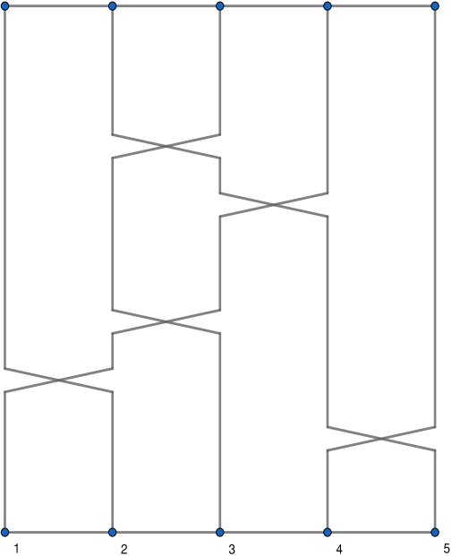
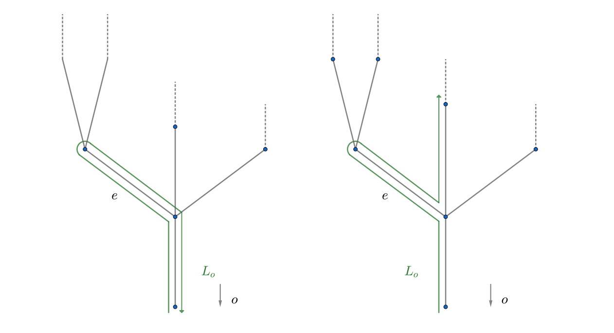
Figure 2: Top: examples of an edge ($\{2,3\}$) and three link configurations so that the edge is pruning, blocking but not pruning, and neither pruning nor blocking, respectively. Bottom left: the effect of a pruning edge $e$ on the path of $L_{o}$ in $T$. Bottom right: the effect of a blocking edge $e$ on the path of $L_{o}$ in $T$.

To formalize the coupling between pruning edges and pruning percolation, we use the notation $\preceq$ to express stochastic domination between measures on rooted trees. When applied to our distributions $\mathsf{loop}_{\beta}[T],\mathsf{link}_{\beta}[T]$, etc., the notion refers to the distribution of the component containing $o$. Note that in the case of loops, this refers to all vertices $L_{o}$ visits. Instead of using the usual partial order on rooted trees to define stochastic domination we define instead the weaker partial order

$$(T,o)\leq(T^{\prime},o^{\prime})\text{ if }e=\{a(x),x\}\in E(T)\text{ implies }e\in E(T^{\prime})\text{ or }T_{a(x)}\in\{K_{1},P_{2}\},$$

where $K_{1}$ is the graph consisting of a single edge and $P_{2}$ is the path consisting of $2$ edges. It is straightforward to see that this ordering suffices for our intended application to questions of percolation, since the removal of finite subtrees has no effect on whether or not $o$ is connected to $\infty$.

Additionally, for percolation processes $\mathsf{A},\mathsf{B}$ on a base graph $G$, we write $\mathsf{B}\circ A[G]$ for the distribution of a percolation configuration obtained by first percolating $G$ with $\mathsf{A}$ and then using the obtained subgraph of $G$ as input for the percolation process $\mathsf{B}$.

Lemma 3.4.

For any tree, we have

$$\mathsf{loop}_{\beta}[T]\preceq\mathsf{delay}_{\beta}\circ\mathsf{link}_{\beta}[T]\preceq\mathsf{link}_{\beta}\circ\mathsf{delay}_{\beta}[T]\preceq\mathsf{link}_{\beta}[T],$$

and consequently $\beta_{\textup{c}}^{\mathsf{loop}}(T)\geq\beta_{\textup{c}}^{\mathsf{link}\circ\mathsf{delay}}(T)\geq\beta_{\textup{c}}^{\mathsf{link}}(T)$.

Proof.

The third relation is trivial. The second relation follows by observing that on one hand, independent percolation processes commute, if the percolation probabilities do not depend on the base graph, and on the other hand performing link percolation first potentially reduces the degrees and thereby reduces the probability that a vertex gets pruned afterward. Henceforth, we only focus on the first relation. For any edge $e\in E$, let $A_{1}(e)$ denote the event that $e$ carries precisely one link. We now work conditionally on the link-cluster $C_{o}$ of $o$ in $T$. Fix any edge $e\in E(C_{o})$ with endpoint $x(e)$ and let $N$ denote the set of offspring of $x(e)$ in $C_{o}$ (i.e. the vertices neighbouring $x(e)$ that are further away from the root then $x(e)$). Assume for the moment that $N$ is nonempty. Let $y^{\ast}$ denote a fixed vertex in $N$ and denote its degree by $D^{\ast}$. Let

$$B(e,y^{\ast})=\big{\{}\{x(e),y^{\ast}\}\text{ is pruning}\big{\}}.$$

Then we have, for $D=\textup{deg}_{C_{o}}(x(e))\geq 2$,

$$\mathsf{loop}_{\beta}[T]\big{(}A_{1}(e)\cap B(e,y^{\ast})|C_{o}\big{)}$$

$$=\frac{\beta\textup{e}^{-\beta}}{1-\textup{e}^{-\beta}}\;\frac{\textup{e}^{-\beta}}{1-\textup{e}^{-\beta}}\frac{\beta^{2}}{2}$$

$$\phantom{space}\times\mathbb{E}\Big{[}\Big{(}\frac{\textup{e}^{-\beta}}{1-\textup{e}^{-\beta}}\sum_{k=1}^{\infty}\frac{\beta^{k}}{k!}(U_{1}\wedge U_{2}+1-U_{1}\vee U_{2})^{k}\Big{)}^{D^{\ast}-1}\Big{(}\frac{\textup{e}^{-\beta}}{1-\textup{e}^{-\beta}}\sum_{k=1}^{\infty}\frac{\beta^{k}}{k!}(U_{1}\vee U_{2}-U_{1}\wedge U_{2})^{k}\Big{)}^{D-2}\Big{]},$$

where $U_{1},U_{2}$ are independent $\operatorname{Uniform}[0,1)$ random variables. The individual terms are explained as follows: in the second line we have the conditional probabilities that $e$ carries precisely one link and that $\{x(e),y^{\ast}\}$ carries precisely two links (recall that we work under the standing assumption that there are only crosses). Note that these events are independent of each other and of the link status of the remaining edges adjacent to $x(e)$ and $y^{\ast}$. The two factors in the expectation correspond to the events that links on the remaining edges adjacent to $\{x(e),y^{\ast}\}$ fall into the complements of the exposed intervals. Note that conditionally on the exposed intervals, these link events are all independent. Finally note that on the event $A_{1}(e)$ we may calculate the positions of the exposed intervals relative to the position of the single link on $e$, which allows the given representation of the length of their complements through $U_{1},U_{2}$.

Gathering terms and setting $\ell=U_{1}\wedge U_{2}+1-U_{1}\vee U_{2}$ yields

$$\mathsf{loop}_{\beta}[T]\big{(}A_{1}(e)\cap B(e,y^{\ast})|C_{o}\big{)}=\frac{\beta^{3}\textup{e}^{-2\beta}}{2(1-\textup{e}^{-\beta})^{2}}\mathbb{E}\Big{[}\Big{(}\frac{\textup{e}^{-\beta}(\textup{e}^{\beta\ell}-1)}{1-\textup{e}^{-\beta}}\Big{)}^{D^{\ast}-1}\Big{(}\frac{\textup{e}^{-\beta}(\textup{e}^{\beta(1-\ell)}-1)}{1-\textup{e}^{-\beta}}\Big{)}^{D-2}\Big{]},$$

which coincides with the definition of $r_{\beta}(x(e)).$

Finally, we observe that we may choose $y^{\ast}$ to be the vertex in $N$ with minimal degree in $C_{o}$ and that the events $\big{(}A_{1}(e)\cap B(e,y^{\ast})$ is independent for different edges as long as they do not lie within distance $2$ of each other on the same path from the root. Hence, we may couple $\mathsf{loop}_{\beta}[T]$ and $\mathsf{delay}_{\beta}[C_{o}]$ in such a way that $L_{o}$ cannot enter any sub-tree $T_{x}$ for which $x$ has been removed in $\mathsf{delay}_{\beta}[C_{o}]$.

∎

We close this section by stating some evident properties of the percolation probabilities $(r_{\lambda}(x)\big{)}_{x\in T\setminus\{o\}}$.

Proposition 3.5.

Fix $u\in[0,1]$. Consider the pruning probability $R(d,d^{\ast},\lambda)$ of a vertex $x$ in a tree $T$ satisfying

$$\deg_{T}(x)=d,D^{\ast}(x)=d^{\ast}.$$

Then $R$ is non-increasing in $d$ and $d^{\ast}$ and continuous in $\lambda\in(0,1)$. We furthermore have

$$R(d,d^{\ast},\lambda)>0\quad\text{ for all }d,d^{\ast}\in\mathbb{N}\cup\{0\},\lambda\in(0,\infty),$$

and

$$\lim_{\lambda\to 0}R(d,d^{\ast},\lambda)=\lim_{\lambda\to\infty}R(d,d^{\ast},\lambda)=\lim_{d\to\infty}R(d,d^{\ast},\lambda)=\lim_{d^{\ast}\to\infty}R(d,d^{\ast},\lambda)=0.$$

Proof.

The observations follow immediately upon inspecting the definition of $(r_{\lambda}(x)\big{)}_{x\in T\setminus\{o\}}$. ∎

4 Loop percolation on Galton-Watson trees

We begin by investigating loop percolation on Galton-Watson trees. Let $T$ denote a Galton-Waltson tree with offspring law $\zeta=(\zeta_{0},\zeta_{1},\dots)$. Clearly, $\beta_{c}^{\mathsf{link}}(T)\equiv\beta_{c}^{\mathsf{link}}(\zeta)$ by Kolmogorov’s $0$–$1$ law and we have

$$\sup\big{\{}\beta\geq 0:\mathsf{link}_{\beta}[T]\big{(}\big{|}\big{(}C_{o}\big{|}<\infty\big{)}=0\big{\}}=-\log\Bigg{(}1-\frac{1}{\sum_{k}k\zeta_{k}}\Bigg{)}.$$

Note that $C_{o}$ can be represented as a Galton-Watson tree with generic offspring variable $X_{\beta}\sim\operatorname{Bin}(X,1-e^{-\beta})$, where $X$ has distribution $\zeta$. To stress the dependence on $\beta$, we denote this tree by $T_{\beta}$ instead of $C_{o}$. Our aim in this section is to prove the following theorem:

Theorem 4.1.

Let $(T,o)$ denote a Galton-Watson tree with offspring law $\zeta$ and probability generating function $f=f_{\zeta}$. Then

1. If $\sum_{k=1}^{\infty}k\zeta_{k}\in(1,\infty)$, then $\beta_{c}^{\mathsf{loop}}(\zeta)>\beta_{c}^{\mathsf{link}}(\zeta)$.

2. If there exists $\varepsilon_{0}>0$ such that

   $$\sqrt{\varepsilon}f^{\prime}(1-\varepsilon)>\tfrac{1}{\sqrt{2}}\quad\text{ for all }\varepsilon\in(0,\varepsilon_{0}),$$ (5)

   then $\beta_{c}^{\textup{loop}}=\beta_{c}^{\textup{link}}=0$. In particular, (5) holds if $\zeta_{k}$ is regularly varying of index $-\tau$ as $k\to\infty$ for any $\tau\in(1,\tfrac{3}{2}).$

3. If $\sum_{k=1}^{\infty}k\zeta_{k}\leq 1$, then $\beta_{c}^{\textup{loop}}=\beta_{c}^{\textup{link}}=\infty$.

Note that we illustrate our use of the couplings presented in Section 3 by providing a short direct proof of Theorem 4.1(i) that is independent of the validity of Theorem A. The restricted setting allows us to highlight the main ideas in an elementary fashion that does not require the machinery discussed in the next section.

Remark 4.2.

• To see that Theorem 4.1(i) is a special case of Theorem A, one needs to change measure from the Galton-Watson measure to the augmented Galton-Watson measure, c.f. [20]

• Condition (5) in Theorem 4.1(ii) can be related to the tail of $\zeta$ via Tauberian theorems, which yields the sufficient condition on the index of variation of $\zeta$: Expanding $\log(1-z)$ around $z=0$, one can see that for $z\in(0,1)$ sufficiently small,

  $$f_{\zeta}(1-z)=\hat{\zeta}(z)\ell(z),$$

  where $\hat{\zeta}(s)=\sum_{k}\textup{e}^{-sk}\zeta_{k}$ denotes the Laplace transform of $\zeta$ and $\ell$ is slowly varying at $0$. One can thus ensure that (5) is satisfied by requiring, for $\alpha>0$ small,

  $$-\frac{\textup{\,{d}}}{\,\textup{d}z}\hat{\zeta}(z)\asymp z^{-\frac{1}{2}-\alpha},\quad\text{ as }{z\to 0},$$ (6)

  and then using Potter bounds. Applying a suitable Tauberian theorem such as [12, XIII.5, Theorem 1], we see that (6) is equivalent to

  $$\sum_{k=1}^{t}k\zeta_{k}\asymp t^{\frac{1}{2}+\alpha},\quad\text{ as }t\to\infty,$$

  i.e. our result covers, for instance, the case in which $\zeta_{k}\asymp k^{-3/2+\alpha}$.

• Condition (5) is far from sharp, but better bounds require a more thorough analysis of the structure of the multi-link loop attached to the root, cf. Proposition 4.5 below. Interestingly, one obtains precisely (5) by replacing our direct argument by the recursive approach of [9], which is strong enough to determine the order of the loop critical value on the $d$-ary tree fairly precisely as $d\to\infty$.

• Our proof blow also shows that if (5) holds, then the phase transition for loop percolation is locally sharp, i.e. there exists an interval $(0,\beta_{0})$ such that an infinite loop exits for all $\beta\in(0,\beta_{0})$ almost surely, conditionally on the survival of $T$.

Proof of Theorem 4.1.

1. We only provide the argument explicitly for $u=1$, the proof goes through, mutatis mutandis, for $u<1$. Let $(T_{\beta},o)$ be a Galton-Watson tree with generic offspring variable $X_{\beta}$, i.e $(T_{\beta},o)$ is the Galton-Watson tree which we obtain from $\mathsf{link}_{\beta}[T]$. Consider $\mathsf{delay}_{\lambda}[T_{\beta}]$ and define a new Galton-Watson tree $(T_{\beta,\lambda},o)$ as follows: vertices of $(T_{\beta,\lambda},o)$ produce offspring according to the distribution of the grandchildren of $o$ in $T_{\beta}$ after performing $\mathsf{delay}_{\lambda}[T_{\beta}]$. The independence of delay percolation, together with the branching property of the Galton-Watson process, implies that $(T_{\beta},o)$ and $\mathsf{delay}_{\lambda}[T_{\beta}]$ can be coupled such that the generations of $(T_{\beta,\lambda},o)$ coincide with the non-delayed generations (all nodes which have not distance $3\mathbb{N}+1$) of the tree component of the root in $\mathsf{delay}_{\lambda}[T_{\beta}]$.

   To be precise, conditionally on $X_{\beta}$ introduce the random variable:

   $$\Gamma(\lambda)\sim\operatorname{Bin}\Bigg{(}X_{\beta},\tfrac{\lambda^{3}\textup{e}^{-2\lambda}}{2(1-\textup{e}^{-\lambda})^{2}}\int_{0}^{1}\int_{0}^{1}\Big{(}\tfrac{\textup{e}^{-\lambda}(\textup{e}^{\lambda(1-|u-v|))}-1)}{1-\textup{e}^{-\lambda}}\Big{)}^{D^{\ast}(o)-1}\Big{(}\tfrac{\textup{e}^{-\lambda}(\textup{e}^{\lambda|u-v|}-1)}{1-\textup{e}^{-\lambda}}\Big{)}^{\deg_{T}(o)-2}\,\textup{d}u\,\textup{d}v\Bigg{)}$$

   corresponding to the number of offspring removed by $\mathsf{delay}_{\lambda}[T_{\beta}]$. The offspring of the root in $(T_{\beta,\lambda},o)$ then has distribution:

   $$\sum_{i=1}^{X_{\beta}-\Gamma(\lambda)}X_{\beta}^{i},$$

   where $X^{i}_{\beta}$ are i.i.d. copies of $X_{\beta}$. Moreover, the offspring of the root in the $\mathsf{delay}_{\lambda}[T_{\beta}]$-perturbed Galton-Watson tree is stochastically dominated by:

   $$\sum_{i=1}^{X_{\beta}}X_{\beta}^{i}-\sum_{i=1}^{X_{\beta}}\Gamma_{i}(\lambda),$$ (7)

   where $\Gamma_{i}(\lambda)$ are i.i.d. copies of $\Gamma(\lambda)$.

   Notice that the expectation of $\mathsf{link}_{\beta}[T]$ is continuous in $\beta$. Therefore, since a Galton-Watson branching process is critical when $\mathbb{E}(X)=1$ we obtain

   $$\lim_{\beta\downarrow\beta_{c}}\mathbb{E}(X_{\beta})=\lim_{\beta\downarrow\beta_{c}}\mathbb{E}(X_{\beta}^{i})=1.$$

   Applying Wald’s Theorem to the first term in Equation (7) yields:

   $$\lim_{\beta\downarrow\beta_{c}}\mathbb{E}\Big{(}\sum_{i=1}^{X_{\beta}}X_{\beta}^{i}\Big{)}=1.$$

   For the second term in Equation (7) we get

   $$\lim_{\beta\downarrow\beta_{c}}\Bigg{(}\sum_{i=1}^{X_{\beta}}\Gamma_{i}(\lambda)\Bigg{)}=\lim_{\beta\downarrow\beta_{c}}\mathbb{E}\big{(}X_{\beta}\big{)}\mathbb{E}\big{(}\Gamma_{1}(\lambda)\big{)}.$$

   Since $\mathbb{E}\big{(}\Gamma_{1}(\lambda)\big{)}>0$ for $\lambda\in(0,\infty)$ the claim of $(i)$ of Theorem 4.1 follows by the continuity of the expectation in $\lambda$ and $\beta$ and by the sub-criticality of the Galton-Watson branching process for $\mathbb{E}X<1$.

2. Consider $(T,o)$ together with its link configuration and denote by $T^{\prime}$ the subtree of $T$ rooted at $o$ that is obtained by considering the root component of $\mathsf{link}_{\beta}[T]$ and then removing every vertex $x\in T$ such that there exists $y$ with $a(y)=0$ such that $e_{y}$ carries more than one link. It is elementary to see, that if $\sharp T^{\prime}=\infty$, then $|L_{o}|=\infty$. Now note that, for given $\beta\in(0,\infty)$, $T^{\prime}$ is a Galton-Watson tree with generic offspring random variable

   $$Y_{\beta}=X_{\beta}\mathbbm{1}_{\{B(X_{\beta},\beta)=0\}},$$

   where conditionally on $X_{\beta}=n$, the random variable $B(X_{\beta},\beta)$ is distributed as $\operatorname{Bin}(n,h(\beta))$ with

   $$h(a)=\frac{\textup{e}^{-a}\sum_{k=2}\frac{a^{k}}{k!}}{1-\textup{e}^{-a}},\quad a>0$$

   i.e. $h(a)=\mathbb{P}(P>1|P>0)$ where $P\sim\operatorname{Poiss}(a)$. Consequently, to decide whether $T^{\prime}$ survives with positive probability, we only need to evaluate $\mathbb{E}[Y_{\beta}]$. To this end we consider the generating function

   $$f_{\beta}(z)=\mathbb{E}[z^{X_{\beta}}],\quad z\in[0,1].$$

   From the definition of $Y_{\beta}$, we obtain using conditional expectations

   $$\mathbb{E}[Y_{\beta}]=\mathbb{E}[X_{\beta}(1-h(\beta))^{X_{\beta}}]=(1-h(\beta))f^{\prime}_{\beta}(1-h(\beta)),$$

   and we need to investigate the asymptotics of this expression as $\beta\downarrow 0$. We use that for small $\beta$

   $$\textup{e}^{-\beta}=1-\beta+\frac{\beta^{2}}{2}+O(\beta^{3}),$$

   and

   $$h(\beta) =\frac{\beta}{2}-\frac{\beta^{2}}{12}+O(\beta^{3}).$$

   Now, using the moment generating function of $\operatorname{Bin}\big{(}X,1-\textup{e}^{-\beta}\big{)}$ and setting $f(z)=\mathbb{E}[z^{X}],\,z\in[0,1]$, we obtain

   $$f_{\beta}^{\prime}(z)=\big{(}1-\textup{e}^{-\beta}\big{)}f^{\prime}\big{(}\textup{e}^{-\beta}+\big{(}1-\textup{e}^{-\beta})z\big{)},$$

   and hence

   $$\mathbb{E}[Y_{\beta}] =\big{(}1-h(\beta)\big{)}\big{(}1-\textup{e}^{-\beta}\big{)}f^{\prime}\big{(}\textup{e}^{-\beta}+\big{(}1-\textup{e}^{-\beta})z\big{)}$$

   $$=\big{(}\beta+O(\beta^{2})\big{)}f^{\prime}\big{(}1-\tfrac{\beta^{2}}{2}+O(\beta^{3})\big{)}.$$

   In particular, it follows that if $\sqrt{2\varepsilon}f^{\prime}(1-\varepsilon)>{1}$ for all $\varepsilon\in(0,\varepsilon_{o})$, then $T^{\prime}$ has a positive probability of survival for all sufficiently small $\beta$, i.e. (ii) is proven.

3. This part is trivial, since if $\sum_{k=1}^{\infty}k\zeta_{k}\leq 1$, then $T$ dies out almost surely, so neither an infinite loop nor an infinite percolation cluster can exist.

∎

Definition 4.3.

For a Galton-Watson tree $T$ with root $o$ consider a vertex $x\in T$. We define the multi-link cluster below $x$ to be the the rooted subtree $(M_{x},x)$ of $T_{x}$ containing $x$ such that every edge in $(M_{x},x)$ has two or more links. In the case where every child $y$ of $x$ has $m_{\{x,y\}}\leq 1$, $(M_{x},x)$ consists of only the isolated vertex $x$. We also define $\gamma_{x}$ to be the loop on $(M_{x},x)$ containing $(x,0)$, we call $\gamma_{x}$ the multi-link loop containing $(x,0)$. This loop only follows links on edges in $(M_{x},x)$, i.e. it ignores any edges with only one link. In the case where $(M_{x},x)$ consists of only the isolated vertex $x$ we have that $\gamma_{x}=\{x\}\times[0,1]$. Lastly, we call a link that is the only link on its edge a uni-link. Note that adding a uni-link to an edge results in a union of the two loops containing its end points.

The following lemma is essentially a mild generalisation of [6, Proposition 3.2].

Lemma 4.4.

Let $T$ be a Galton-Watson tree with root $o$ and let $C^{(1)}(o)$ be the number of uni-links incident to the support of $\gamma_{0}$, the multi-link loop containing $(o,0)$. The loop $\gamma$ containing $(o,0)$ is infinite with positive probability if and only if $\mathsf{loop}_{\beta}[T](C^{(1)}(o))>1$.

Proof.

We proceed with an exploration of the loop $\gamma$ containing $(o,0)$ as follows. We consider the loop as starting at $(o,0)$ by crossing a uni-link from a parent vertex $g$ such that $o$ is the only child of $g$. When following $\gamma$, if we encounter a uni-link to a new vertex $x$ we sample the multi-link sub-tree, $(M_{x},x)$, with root $x$. Our exploration of $\gamma$ now crosses this uni-link which merges it with a loop with the same distribution as $\gamma_{x}$, the multi-link loop containing $(x,0)$ (to see this note that we can apply a time shift to each vertex of $(M_{x},x)$ so that $\gamma$ arrives at time $0$). While following $\gamma_{x}$ we may encounter other uni-links, in which case we will move to a new vertex not in $(M_{x},x)$ to sample a new multi-link sub-tree. The number of uni-links attached to $\gamma_{x}$ has the same distribution as $C^{(1)}(0)$.

We can hence introduce a new Galton-Watson tree $(\tilde{T},\tilde{o})$ where we map $o$ to $\tilde{o}$ and offspring of $\tilde{o}$ in $\tilde{T}$ are vertices $x\in T$ with uni-links attached to $\gamma_{o}$ (excluding the one we crossed to enter $\gamma_{o}$). Each child has its own multi-link sub-tree and offspring with the same distribution as for $\tilde{o}$. The offspring distribution is therefore given by $C^{(1)}(o)$.

The loop exploration can be coupled to $(\tilde{T},\tilde{o})$ as each time we reach a new vertex $x$ via a uni-link we will enter a loop distributed as $\gamma_{x}$ which we leave via a newly discovered uni-link or by backtracking to $a(x)$ to further explore $\gamma_{x}$. If $(\tilde{T},\tilde{o})$ does not become extinct this loop exploration will continue forever. We now see that $\mathsf{loop}_{\beta}[T](C^{(1)}(o))>1$ is necessary and sufficient for $(\tilde{T},\tilde{o})$ to be supercritical.

To complete the argument, we need to show that survival of $(\tilde{T},\tilde{o})$ is the only way that $\gamma$ can be infinite. We need only exclude the possibility $\gamma_{o}$ is infinite with positive probability but encounters at most one uni-link in expectation conditionally on being infinite. Let us argue that this cannot happen, in fact this conditional expectation is infinite and hence $\mathsf{loop}_{\beta}[T](C^{(1)}(o))=\infty$ if $\mathsf{loop}_{\beta}[T](|\gamma_{o}|=\infty)>0$. Consider the event $G_{\varepsilon}(x)$ that $\gamma_{o}$ spends time at least $\varepsilon>0$ at the vertex $x$ and $x$ has at least one uni-link child. By the ergodic theorem, the probability $\mathsf{loop}_{\beta}[T](G_{\varepsilon}(x)\,|\,|\gamma_{o}|=\infty,x\in\gamma_{o})$ converges as $|x|\to\infty$ to some value $G>0$ for $\varepsilon$ sufficiently small. Conditional on the event $G_{\varepsilon}(x)$, the expected number of uni-links connecting to $\gamma_{o}$ at $x$ is at least $\varepsilon>0$. We hence see that we must have $\mathsf{loop}_{\beta}[T](C^{(1)}(o))=\infty$. ∎

We now consider the case where the offspring law $\zeta$ is Poisson($\lambda$).

Proposition 4.5.

Suppose that $T$ is a Galton-Watson tree with root $o$ and offspring distribution $X\sim$ Poisson$(\lambda)$. Then the loop containing $(o,0)\gamma$ if infinite with positive probability if and only if

$$\mathsf{loop}_{\beta}[T](|\gamma_{o}|)\beta e^{-\beta}\lambda>1.$$

In the case $u=1$ loops have lengths in $\mathbb{N}$ so that a sufficient condition for the existence of infinite loops with positive probability is $\beta e^{-\beta}\lambda>1$.

Proof.

In this case we can sample the multi-link subtree of $o$ independently of the uni-links. An edge has two or more links with probability $(1-(1+\beta)e^{-\beta})$ and a uni-link with probability $\beta e^{-\beta}$ so that we can think of $T_{\beta}$ as a multi-type Galton-Watson tree with independent offspring types, 0, 1, and $2+$ each with Poisson distributions of rates $e^{-\beta}\lambda$, $\beta e^{-\beta}\lambda$, and $(1-(1+\beta)e^{-\beta})\lambda$, respectively. Hence

$$\mathsf{loop}_{\beta}[T](C^{(1)}(o))=\mathsf{loop}_{\beta}[T](|\gamma_{o}|)\beta e^{-\beta}\lambda$$

and by Lemma 4.4 we have the result. ∎

5 Potential theory and percolation on trees

We call a self-avoiding path $\xi=(o,\xi_{1},\xi_{2},\dots)$ in $T$ a ray, if it cannot be extended. Two rays $\xi,\xi^{\prime}$ are equivalent if $\sharp(\{\xi_{i},i\in\mathbb{N}\}\Delta\{\xi^{\prime}_{i},i\in\mathbb{N}\})<\infty$ and the set of equivalence classes of rays $\partial T$ is called the boundary of $T$. We will not notationally distinguish between rays and their equivalence classes. For $\xi,\xi^{\prime}\in\partial T$, define $\xi\wedge\xi^{\prime}$ to be the vertex furthest away from the root that is common to both $\xi$ and $\xi^{\prime}$. Then $(\xi,\xi^{\prime})\mapsto\textup{e}^{-|\xi\wedge\xi^{\prime}|}$ defines a metric on $\partial T$ with respect to which the boundary forms a complete separable metric space. As in the introduction, we write $\dim(X)$ for the Hausdorff dimension of a metric space $X$.

To study more general trees than Galton-Watson trees, we use the powerful machinery of harmonic analysis on trees and its connection with percolation, which was developed in [17, 18, 19]. Our presentation relies mostly on the monograph [20]. Consider a rooted infinite tree $(T,o)$. A function $g:T\to[0,\infty)$ on the vertices of $T$ is called a gauge if it is non-decreasing along rays. By monotonicity, we may thus extend any gauge to a function on $\partial T\to[0,\infty]$, which we also denote by $g$. A gauge $g$ gives rise to a kernel $\mathscr{k}_{g}:\partial T\times\partial T\to[0,\infty]$ via

$$\mathscr{k}_{g}(\xi,\xi^{\prime})=g(\xi\wedge\xi^{\prime}).$$

By $\Delta g$ we denote the function $g(x)-g(a(x))\geq 0,x\neq o$, i.e. the gauge difference between $x$ and its parent. We may think of $\Delta g$ as a cost or resistance encountered when traversing the edge $\{a(x),x\}$ from the root and indeed this notion can be made rigorous using the electrical network formalism, see [20]. Consequently, $\Delta g$ can also be interpreted as a function of the edges in $T$, which is occasionally convenient. Recall that the boundary $\partial T$ of $T$ carries a metric structure and we can thus define

$$\Pi(\partial T)=\{\nu:\nu\text{ is a Borel measure on }\partial T\text{ with }\nu(\partial T)=1\}.$$

The potential of $\nu\in\Pi(\partial T)$ with respect to the gauge $g$ is defined as

$$\mathscr{h}_{g,\nu}(\xi)=\int_{\partial T}\mathscr{k}_{g}(\xi,\xi^{\prime})\nu(\textup{d}\xi^{\prime}),\quad\xi\in\partial T,$$

and the corresponding energy is

$$\mathscr{E}_{g}(\nu)=\int_{\partial T\times\partial T}\mathscr{k}_{g}(\xi,\xi^{\prime})\nu\otimes\nu(\textup{d}\xi,\textup{d}\xi^{\prime})=\int_{\partial T}\mathscr{h}_{g,\nu}(\xi)\nu(\textup{d}\xi).$$

The following alternative representation of the potential was established in [17], cf. [20, Prop. 16.1],

$$\mathscr{h}_{g,\nu}(\xi)=\sum_{x\in\xi}\Delta g(x)\nu(b_{x}),$$ (8)

where the ball $b_{x}\subset\partial T$ around $x\in T$ consists of those rays $\xi\in\partial T$ that contain $x$.

Finally, the $g$-capacity of a Borel set $A\subset\partial T$ is the quantity

$$\mathscr{C}_{g}(A)=\inf\{\mathscr{E}_{g}(\nu):\nu\in\Pi(\partial T),\,\operatorname{supp}(\nu)=A\}^{-1}.$$

The connection of these potential theoretic notions with independent Bernoulli percolation is as follows: any independent Bernoulli percolation on $T$ can be parametrised through its edge retention probabilities

$$p(e),e\in T,$$

which gives rise to a gauge function $g_{p}$ via $g_{p}(o)=1$ and

$$g_{p}(x)=\prod_{o<v\leq x}p(e(v))^{-1},\quad x\in T\setminus\{o\},$$

where $v<x$ if $v$ is on the unique path connecting $x$ to $o$ in $T$. Note that $g_{p}(x)$ corresponds precisely to the probability that $x$ can be reached from $o$ in a realisiation of bond percolation with edge retention probabilities given by $p=(p(e),e\in T)$. We call $g_{p}$ the gauge adapted to the independent percolation $(p(e),e\in T)$.

A well-known theorem of Lyons [18] now implies that

$$\mathscr{C}_{g_{p}}(\partial T)\leq\mathbb{P}(\sharp C_{o}=\infty)\leq 2\mathscr{C}_{g_{p}}(\partial T),$$ (9)

where $C_{o}$ is the cluster of $o$ obtained by performing $p$-Bernoulli percolation on $T$. Hence, our strategy is to use a similar coupling idea as in the proof of Theorem 4.1, but to relate the independent percolation measures involved not to mean offspring numbers as in the case of Galton-Watson trees, but to capacities of boundary sets, as these are now the sufficient statistics of the tree to decide whether percolation occurs or not.

In the particular case where $p(e)\equiv p_{\beta}=1-e^{-\beta}$, i.e. the percolation process in question is $\mathsf{link}_{\beta}[T]$, we need to consider the family of purely exponential gauge functions $\{g(x)=r^{|x|},r>1\}$, which we parametrise as $\bar{q}(x)=q^{-|x|}$ with $q\in(0,1)$ for notational convenience. This yields the characterisation

$$\beta_{c}^{\mathsf{link}}(T)=\inf\{\beta\geq 0:\mathscr{C}_{\bar{p}_{\beta}}(\partial T)>0\}$$

of the critical bond percolation probability of $T$ in terms of $\beta$. Another, sometimes more convenient, characterisation of this critical value is via the branching number of $T$

$$\operatorname{br}(T):=\sup\{1/q:\mathscr{C}_{\bar{q}}(\partial T)>0,q\in(0,1)\}=(1-\textup{e}^{\beta_{c}^{\mathsf{link}}(T)})^{-1},$$

which is also intimately related to recurrence and transience of biased random walks on $T$ via their interpretation in terms of electrical networks. Lyons [17] further established the relation

$$\dim(\partial T)=\log(\operatorname{br}(T))$$

for all infinite trees which is the general version of Hawke’s theorem.

We have already seen that a supercritical percolation $(p(e),e\in T)$ is characterised by positive $g_{p}$-capacity, which means that there exist probability measures on $\partial T$ with finite energy. In fact, Dirichlet’s principle yields

$$\mathscr{C}_{g_{p}}(\partial T)>0\text{ if and only if there exists a unique minimiser }\nu_{g_{p}}\text{ of }\{\mathscr{E}_{g_{p}}(\nu):\nu\in\Pi(\partial T)\}.$$ (10)

The measure $\nu_{g_{p}}$ is called the harmonic measure of $g_{p}$ (or of $(p(e),e\in T)$), it corresponds to the hitting distribution at $\partial T$ for the weighted random walk on $T$ that starts at $o$ and is uniquely defined by the transition probabilities

$$\pi(a(x),x)=\frac{1/\Delta g_{p}(e(x))}{1/\Delta g_{p}(e(a(x)))+\sum_{y:a(y)=a(x)}1/\Delta g_{p}(e(y))},$$

in particular it exists if and only if the walk is transient. The following lemma allows us to infer almost sure results about weighted random walks from almost sure results of simple random walk.

Lemma 5.1.

Let $(T,o)$ be an infinite rooted tree and let $g_{1},g_{2}$ be two gauges on $T$ such that

$$\Delta g_{1}(x)\geq\Delta g_{2}(x)\geq 1\text{ for all but finitely many }x\in T\setminus\{o\}.$$

Denote the corresponding harmonic measures by $\nu_{1}$ and $\nu_{2}$ and let $\mathscr{E}_{1},\mathscr{E}_{2}$ denote the respective energies. Then we have

1. $\nu_{1}\ll\nu_{2}$;

2. if $\nu$ is any Borel probability measure on $B\subset{\partial T}$ with $\mathscr{E}_{1}(\nu)<\infty$, then $\nu\ll\nu_{2}(\,\cdot\,|B)$.

Proof.

It suffices to consider the system of balls $b_{x}=\{\xi\in\partial T:x\in\xi\},\,x\in T$ generating the Borel $\sigma$-field of $\partial T$. Fix any ball with $\nu_{1}(b_{x})>0$. The conditional measure on $b_{x}$

$$\nu_{1}^{x}(\,\cdot\,)=\frac{\nu_{1}(\,\cdot\,\cap\,b_{x})}{\nu_{1}(b_{x})}$$

exists and it is not difficult to see that this is the $g_{1}$-harmonic measure on $\partial T_{x}$, where $T_{x}$ is the subtree of $T$ rooted at $x$. If $\nu$ is any Borel probability measure on $b_{x}=\partial T_{x}$, then we have

$$\mathcal{E}_{1}(\nu_{1}^{x})=\inf_{\mu}\mathcal{E}_{1}(\mu)\leq\mathcal{E}_{1}(\nu),$$ (11)

where the infimum runs over all Borel probability measures $\mu$ on $b_{x}$. Also, from Rayleigh’s monotonicity principle (see [20, Prop. 16.1] for the precise version for energies) it follows that $\mathcal{E}_{2}(\mu)\leq\mathcal{E}_{1}(\mu)$ for any Borel probability measure $\mu$ on $b_{x}$. Hence

$$\inf_{\mu}\mathcal{E}_{2}(\mu)\leq\mathcal{E}_{2}(\nu_{1}^{x})\leq\mathcal{E}_{1}(\nu_{1}^{x})\leq\mathcal{E}_{1}(\nu).$$

Consequently, if either one of the last two terms is finite, then $\mathcal{E}_{2}(\nu_{1}^{x})$ is finite. In this case the $g_{2}$-harmonic measure $\nu_{2}^{x}$ on $b_{x}$, which is the minimiser of the $g_{2}$-energy, is then a well-defined finite measure. In particular, since for any Borel set $A\subset b_{x}$ we have

$$\nu_{2}^{x}(A)=\frac{\nu_{2}(A)}{\nu_{2}(b_{x})},$$

it then follows that $\nu_{2}(b_{x})>0$. Since $b_{x}$ was arbitrary with $\nu_{1}(b_{x})>0$, the proof is complete. ∎

We close this section with the following two results, needed in the proof Theorem A.

Lemma 5.2.

Let $(G,o)$ be any infinite connected rooted graph and let $X=(X_{n})_{n\geq 0}$ denote a transient (not necessarily symmetric) nearest neighbour random walk on $G$ with $X_{0}=o$. Define

$$\tau_{k}=\max\{n\in\mathbb{N}:S_{n}\in B_{G}(o,k)\},\quad k\in\mathbb{N},$$

the last exit times of $X$ from the balls of radius $k$ around $o$. Then

$$\liminf_{n\to\infty}\frac{\operatorname{dist}_{G}(X_{n},o)}{n}=\liminf_{k\to\infty}\frac{k}{\tau_{k}}\leq\limsup_{n\to\infty}\frac{\operatorname{dist}_{G}(X_{n},o)}{n},$$

and, in particular, almost sure existence of the speed $\lim_{n\to\infty}\frac{\operatorname{dist}_{G}(X_{n},o)}{n}=s(X)$ implies that almost surely

$$\lim_{k\to\infty}\frac{\tau_{k}}{k}=\frac{1}{s(X)}\in(1,\infty].$$

Proof.

The chain of inequalities

$$\liminf_{n\to\infty}\frac{\operatorname{dist}_{G}(X_{n},o)}{n}\leq\liminf_{k\to\infty}\frac{k}{\tau_{k}}\leq\limsup_{k\to\infty}\frac{k}{\tau_{k}}\leq\limsup_{n\to\infty}\frac{\operatorname{dist}_{G}(X_{n},o)}{n},$$

follows immediately upon noticing that

$$\frac{\operatorname{dist}_{G}(X_{\tau_{k}},o)}{\tau_{k}}=\frac{k}{\tau_{k}},\quad k\in\mathbb{N}.$$

Now, for $n\in\mathbb{N}$, set $K(n)$ to be the unique index $k$ for which $\tau_{k}\leq n<\tau_{k+1}$ and observe that

$$\frac{\operatorname{dist}_{G}(X_{n},o)}{n}\geq\frac{K(n)}{\tau_{K(n)+1}}=\frac{K(n)+1}{\tau_{K(n)+1}}\frac{K(n)}{K(n)+1},$$

i.e.

$$\liminf_{n\to\infty}\frac{\operatorname{dist}_{G}(X_{n},o)}{n}\geq\liminf_{k\to\infty}\frac{k}{\tau_{k}},$$

from which the lemma follows. ∎

A percolation process $\mathsf{P}$ on a rooted tree $(G,o)$ is called adapted, if it is distributionally invariant under rooted graph automorphisms of $(G,o)$. For instance, $\mathsf{link}_{\lambda},\mathsf{prune}_{\lambda}$ and $\mathsf{loop}_{\lambda}$ are all adapted to the respective base graphs. We furthermore say that $\mathsf{P}$ is finite range if there exists some $K$, such that percolation configurations induced by $\mathsf{P}[G]$ inside subgraphs $H,H^{\prime}$ of $G$ are independent whenever $\operatorname{dist}_{G}(H,H^{\prime})>K$.

The following result is the main ingredient in our proof of Theorem A

Theorem 5.3.

Let $(T,o)\in\mathscr{T}_{\ast}$ be a stationary, ergodic and ballistic random tree with $\operatorname{br}(T)<\infty$ and let $\mathsf{P}$ denote any adapted, finite range percolation on $T$. Furthermore let $F_{\mathsf{P}}$ denote the random forest obtained by realising $\mathsf{P[T]}$ and assume that $\mathsf{P[T]}(e\in F_{\mathsf{P}})<1$ for all $e\in T$. Then

$$\operatorname{br}(T_{\mathsf{P}})<\operatorname{br}(T),$$

where $T_{\mathsf{P}}$ denotes the component of $F_{\mathsf{P}}$ containing $o$.

Proof.

Let $K$ exceed the maximum range of dependence of $\mathsf{P}$. Consider the independent percolation process $\tilde{\mathsf{P}}$ on $(T,o)$ induced by $\mathsf{P}$ via

$$p_{e}:=\mathbbm{1}_{\{|x(e)|\notin K\mathbb{N}+1\}}+\mathbbm{1}_{\{|x(e)|\in K\mathbb{N}+1\}}\mathsf{P}[T](e\in F_{\mathsf{P}}),$$

where $F_{\mathsf{P}}$ denotes a generic realisation of $\mathsf{P}[T].$ By the obvious coupling, we have $\mathsf{P}[T]\preceq\tilde{\mathsf{P}}[T]$ and hence it suffices to show

$$\operatorname{br}(T_{\tilde{\mathsf{P}}})<\operatorname{br}(T),$$ (12)

for the root component $T_{\tilde{\mathsf{P}}}$ of $F_{\tilde{\mathsf{P}}}$.

Our overall strategy to show (12) uses the fact that $\tilde{\mathsf{P}}[T]$ is an independent percolation and can thus be analysed easily using the potential theoretic machinery introduced above. In particular, we will demonstrate that for the induced harmonic measure on $\partial T$ the vertices on which $p$ is bounded away from $1$ have positive density in almost every ray.

Let us call a vertex $x\in T$ $\delta$-exposed if

$$\mathsf{P}[T](e\in F_{\mathsf{P}})\leq 1-\delta.$$ (13)

By stationarity and ergodicity, we have that

$$\lim_{n\to\infty}\frac{1}{n}\sum_{i=1}^{n}\mathbbm{1}_{\{\{S_{i},S_{i-1}\}\text{ is }\delta\text{-exposed}\}}=\mathbb{P}(\{o,S_{1}\}\text{ is }\delta\text{-exposed}).$$

On the other hand, by tightness of the distribution of $(T,o)$, for every $\varepsilon>0$, there exists some finite set $\mathcal{K}\subset\mathscr{T}_{\ast}$ with

$$\mathbb{P}((T,o)\in\mathcal{K})>1-\varepsilon.$$

In particular, since $p_{e}<1$ for all $e\in T$, we can find for every $\varepsilon>0$ a $\delta(\varepsilon)$ such that

$$\mathbb{P}\Big{(}\bigcap_{y\in T:a(y)=o}\{\{o,y\}\text{ is }\delta(\varepsilon)\text{-exposed}\}\Big{)}\geq 1-\varepsilon.$$ (14)

Given $(T,o)$, we assign to a realisation $S$ of simple random walk its loop erasure $\xi(S)$, which we identify with the corresponding ray in $\partial T$. Lemma 5.2 now implies that $\xi(S)$ has asymptotic density $s$ in the range of $S$. Furthermore,

$$\lim_{n\to\infty}\frac{\sharp(\xi_{n}(S)\cap\{x\in T:|x|\in K\mathbb{N}+1\})}{n}=\frac{s}{K}>0,$$ (15)

where $\xi_{n}(S)=(o,\xi_{1}\dots,\xi_{\max\{k\in\mathbb{N}:\tau_{k}\leq n\}})$ corresponds to the initial segment of $\xi(S)$ that has been revealed by time $n$. The pigeon hole principle now implies that we can choose $\varepsilon$ so small that (14) and (15) together imply

$$\liminf_{n\to\infty}\frac{\sharp\{i\leq n:\xi_{i}\in K\mathbb{N}+1,\{\xi_{i},\xi_{i+1}\}\text{ is }\delta(\varepsilon)\text{-exposed}\}}{n}>0.$$ (16)

Having established (16), we now let $f_{\lambda}$ denote the gauge corresponding to $\mathsf{link}_{\lambda}\circ\tilde{\mathsf{P}}$ on $(T,o)$. Note that $f$ is a product of the purely exponential gauge $\bar{p}_{\lambda}$ and the gauge adapted to $\tilde{\mathsf{P}}$. Assume, for contradiction, that equality holds in (12), then

$$\log\Big{(}1-\frac{1}{\operatorname{br}(T_{\tilde{\mathsf{P}}})}\Big{)}=\log\Big{(}1-\frac{1}{\operatorname{br}(T_{\mathsf{P}})}\Big{)}=\beta_{c}^{\mathsf{link}}(T).$$

In particular, this implies that $\partial T$ has finite $f_{\lambda}$-capacity for all $\lambda$ in a right neighbourhood $(\beta_{c}^{\mathsf{link}},\beta_{c}^{\mathsf{link}}+\varepsilon_{0})$ of $\beta_{c}^{\mathsf{link}}$. Consequently, for $\lambda\in(\beta_{c}^{\mathsf{link}},\beta_{c}^{\mathsf{link}}+\varepsilon_{0})$

$$\infty>\mathscr{E}_{f_{\lambda}}(\nu_{f_{\lambda}})=\int_{\partial T}\mathscr{h}_{f_{\lambda},\nu_{f_{\lambda}}}(\xi)\nu_{f\lambda}(\textup{d}\xi).$$ (17)

By (8), the integrand on the right hand side satisfies

$$\mathscr{h}_{f_{\lambda},\nu_{f_{\lambda}}}(\xi)\geq\sum_{\begin{subarray}{c}x\in\xi\\ x\text{ is }\delta\text{-exposed}\end{subarray}}\Delta\overline{(1-\delta)p_{\lambda}}(x)\nu_{f\lambda}(b_{x}),$$

by the definition of the exposed set.

From (15) we now conclude that the collection of $\xi\in\partial T$ that contains only finitely many non-$\delta$-exposed vertices has simple-random-walk harmonic measure $1$ for $\delta=\delta(\varepsilon)$, if $\varepsilon$ is sufficiently small. By Lemma 5.1, this is also true for $\nu_{f_{\lambda}}$-almost every $\xi$. Hence from the bound

$$\mathscr{E}_{f_{\lambda}}(\nu_{f_{\lambda}})=\int_{\partial T}\mathscr{h}_{f_{\lambda},\nu_{f_{\lambda}}}(\xi)\nu_{f_{\lambda}}(\textup{d}\xi)\geq\int_{\partial T}\sum_{\begin{subarray}{c}x\in\xi\\ x\text{ is }\delta\text{-exposed}\end{subarray}}\Delta\overline{(1-\delta)p_{\lambda}}(x)\nu_{f_{\lambda}}(b_{x})\nu_{f_{\lambda}}(\textup{d}\xi),$$ (18)

which contradicts (17) and the characterisation of $\beta_{c}^{\mathsf{link}}<\infty$ via purely exponential gauges. Thus we conclude that (12) must hold. ∎

6 Proof of Theorem A

Finally, we now use the machinery set up in the previous section to prove Theorem A.

Proof of Theorem A.

The argument is essentially identical to the proof of Theorem 5.3. We can apply the reasoning of that proof to the percolation $\mathsf{P}$ induced by the pruning edges under $\mathsf{loop}_{\lambda}[T]$, and the result will follow by Lemma 3.4, since we can set the range bound to $K=3$ and the induced independent percolation $\tilde{\mathsf{P}}$ is precisely $\mathsf{delay}_{\lambda}$. There is only one added subtlety compared with the proof of Theorem 5.3: Varying $\lambda\in(\beta_{c}^{\mathsf{link}(T)},\beta_{c}^{\mathsf{link}(T)}+\varepsilon_{0})$ affects both the parameters in $\mathsf{link}_{\lambda}\circ\mathsf{delay}_{\lambda}$. In particular (18) becomes

$$\mathscr{E}_{f_{\lambda}}(\nu_{f_{\lambda}})=\int_{\partial T}\mathscr{h}_{f_{\lambda},\nu_{f_{\lambda}}}(\xi)\nu_{f_{\lambda}}(\textup{d}\xi)\geq\int_{\partial T}\sum_{\begin{subarray}{c}x\in\xi\\ x\text{ is }\delta\text{-exposed}\end{subarray}}\Delta\overline{(1-\delta(\lambda))p_{\lambda}}(x)\nu_{f_{\lambda}}(b_{x})\nu_{f_{\lambda}}(\textup{d}\xi),$$

and we need to ensure that $\delta(\lambda)=\delta(\varepsilon,\lambda)$ can be uniformly bounded away from $0$ as $\lambda\downarrow\beta_{c}^{\mathsf{link}}(T)$. To this end, we employ Proposition 3.5 to deduce that as $\lambda\downarrow\beta_{c}^{\mathsf{link}}(T)$, the corresponding percolation probabilities converge to those of $\mathsf{prune}_{\beta_{c}^{\mathsf{link}}(T)}$, which are bounded away from $1$ under our standing assumption that $\beta_{c}^{\mathsf{link}}(T)\in(0,\infty).$ ∎

Acknowledgement. We thank Volker Betz for sharing his insights on the loop model and his helpful comments on the first draft of the manuscript. We further thank Daniel Ueltschi for inspiring discussions and hosting AK’s visit to Warwick in February 2025.

References

Funding acknowledgement. CM’s research is funded by Deutsche Forschungsgemeinschaft (DFG, German Research Foundation) – SPP 2265 443916008. AK’s research is funded by the Cusanuswerk e.V.

References

- [1] Michael Aizenman and Bruno Nachtergaele “Geometric aspects of quantum spin states” In Comm. Math. Phys. 164.1, 1994, pp. 17–63 DOI: 10.1007/bf02108805
- [2] David Aldous and Russell Lyons “Processes on unimodular random networks” In Electron. J. Probab. 12, 2007, pp. no. 54\bibrangessep1454–1508 DOI: 10.1214/EJP.v12-463
- [3] Omer Angel “Random infinite permutations and the cyclic time random walk” In Discrete random walks (Paris, 2003) AC, Discrete Math. Theor. Comput. Sci. Proc. Assoc. Discrete Math. Theor. Comput. Sci., Nancy, 2003, pp. 9–16 DOI: 10.46298/dmtcs.3342
- [4] Itai Benjamini and Nicolas Curien “Ergodic theory on stationary random graphs” In Electron. J. Probab. 17, 2012, pp. no. 93\bibrangessep20 pages DOI: 10.1214/EJP.v17-2401
- [5] Volker Betz, Johannes Ehlert and Benjamin Lees “Phase transition for loop representations of quantum spin systems on trees” In J. Math. Phys. 59.11, 2018, pp. Paper no. 113302\bibrangessep13 pages DOI: 10.1063/1.5032152
- [6] Volker Betz, Johannes Ehlert, Benjamin Lees and Lukas Roth “Sharp phase transition for random loop models on trees” In Electron. J. Probab. 26, 2021, pp. Paper No. 133\bibrangessep26 pages DOI: 10.1214/21-ejp677
- [7] Volker Betz, Andreas Klippel and Mino Nicola Kraft “Loop percolation versus link percolation in the random loop model”, 2024 arXiv: https://arxiv.org/abs/2408.00648
- [8] Jakob E. Björnberg, Michał Kotowski, Benjamin Lees and Piotr Miłoś “The interchange process with reversals on the complete graph” In Electron. J. Probab. 24, 2019, pp. Paper No. 108\bibrangessep43 pages DOI: 10.1214/19-ejp366
- [9] Jakob E. Björnberg and Daniel Ueltschi “Critical parameter of random loop model on trees” In Ann. Appl. Probab. 28.4, 2018, pp. 2063–2082 DOI: 10.1214/17-AAP1315
- [10] Jakob E. Björnberg and Daniel Ueltschi “Critical temperature of Heisenberg models on regular trees, via random loops” In J. Stat. Phys. 173.5, 2018, pp. 1369–1385 DOI: 10.1007/s10955-018-2154-2
- [11] Dor Elboim and Allan Sly “Infinite cycles in the interchange process in five dimensions”, 2024 arXiv: https://arxiv.org/abs/2211.17023
- [12] William Feller “An Introduction to Probability Theory and its Applications. Vol. II” John Wiley & Sons, Inc., New York-London-Sydney, 1971, pp. xxiv+669
- [13] Alan Hammond “Infinite cycles in the random stirring model on trees” In Bull. Inst. Math. Acad. Sin. (N.S.) 8.1, 2013, pp. 85–104
- [14] Alan Hammond and Milind Hegde “Critical point for infinite cycles in a random loop model on trees” In The Annals of Applied Probability 29.4 Institute of Mathematical Statistics, 2019, pp. 2067–2088 DOI: 10.1214/18-AAP1442
- [15] T.. Harris “Nearest-neighbor Markov interaction processes on multidimensional lattices” In Advances in Math. 9, 1972, pp. 66–89 DOI: 10.1016/0001-8708(72)90030-8
- [16] Roman Kotecký, Piotr Miłoś and Daniel Ueltschi “The random interchange process on the hypercube” In Electron. Commun. Probab. 21, 2016, pp. Paper No. 4\bibrangessep9 DOI: 10.1214/16-ECP4540
- [17] Russell Lyons “Random walks and percolation on trees” In Ann. Probab. 18.3, 1990, pp. 931–958 DOI: 10.1214/aop/1176990730
- [18] Russell Lyons “Random walks, capacity and percolation on trees” In Ann. Probab. 20.4, 1992, pp. 2043–2088 DOI: 10.1214/aop/1176989540
- [19] Russell Lyons, Robin Pemantle and Yuval Peres “Ergodic theory on Galton-Watson trees: speed of random walk and dimension of harmonic measure” In Ergodic Theory Dynam. Systems 15.3, 1995, pp. 593–619 DOI: 10.1017/S0143385700008543
- [20] Russell Lyons and Yuval Peres “Probability on trees and networks” 42, Cambridge Series in Statistical and Probabilistic Mathematics Cambridge University Press, New York, 2016, pp. xv+699 DOI: 10.1017/9781316672815
- [21] Piotr Miłoś and Batı Şengül “Existence of a phase transition of the interchange process on the Hamming graph” In Electron. J. Probab. 24, 2019, pp. Paper No. 64\bibrangessep21 pages DOI: 10.1214/18-EJP171
- [22] Peter Mühlbacher “Critical parameters for loop and Bernoulli percolation” In ALEA Lat. Am. J. Probab. Math. Stat. 18.1, 2021, pp. 289–308 DOI: 10.30757/alea.v18-13
- [23] Robert T. Powers “Heisenberg model and a random walk on the permutation group” In Lett. Math. Phys. 1.2, 1975/76, pp. 125–130 DOI: 10.1007/BF00398374
- [24] Oded Schramm “Compositions of random transpositions” In Israel J. Math. 147, 2005, pp. 221–243 DOI: 10.1007/BF02785366
- [25] Bálint Tóth “Improved lower bound on the thermodynamic pressure of the spin Heisenberg ferromagnet” In Lett. Math. Phys. 28.1, 1993, pp. 75–84 DOI: 10.1007/BF00739568
- [26] Daniel Ueltschi “Random loop representations for quantum spin systems” In J. Math. Phys. 54.8, 2013, pp. Paper No. 083301\bibrangessep40 pages DOI: 10.1063/1.4817865