A semi-cosmographic approach to study cosmological evolution in phase space

Abstract

The signature of Baryon Acoustic Oscillation in the clustering of dark-matter tracers allows us to measure $(D_{A}(z),H(z))$ independently. Treating these as conjugate variables, we are motivated to study cosmological evolution in the phase space of dimensionless variables $x=H_{0}D_{A}/c$ and $p=dx/dz$. The dynamical system $(x(z),p(z))$ can be integrated for a known set of equation of state parameters for different matter/energy components. However, to avoid any preference for specific dark energy models, we adopt a cosmographic approach. We consider two scenarios where the Luminosity distance is expanded as Padé rational approximants using expansion in terms of $z$ and $(1+z)^{1/2}$ respectively. However, instead of directly using the Padé ratios to fit kinematic quantities with data, we adopt an alternative approach where the evolution of the cold dark matter sector is incorporated in our analysis through a semi-cosmographic equation of state, which is then, used to solve the dynamical problem in the phase space. The semi-cosmographic $(D_{A}(z),H(z))$, thus obtained, is fitted with BAO and SNIa data from DESI DR1 + eBOSS and Pantheon+ respectively. We also consider a futuristic 21-cm intensity mapping experiment for error projections. We further use the semi-cosmographic fitting to reconstruct some diagnostics of background cosmology and compare our results for the two scenarios of Padé expansions.

I Introduction

There is compelling observational evidence for the accelerated expansion of the Universe from a host of cosmological probes [1, 2, 3, 4, 5, 6, 7]. However, a theoretical understanding of dark energy [8, 9, 10, 11] as a potential cause for this cosmic acceleration remains largely uncertain even today. Although, the widely recognized framework of the $\Lambda$CDM model [8, 12, 13] provides the broad cosmological paradigm, a closer scrutiny indicates theoretical challenges [14, 15, 9] and tension with observed data [16, 17, 18, 19, 20, 21]. Notable here is the Hubble-tension which indicates that the value of $H_{0}$ measured implicitly from high redshift CMBR observation [22, 23, 24, 25, 26, 27, 28], Baryon Acoustic Oscillation (BAO) signature (in galaxy clustering [29] or in the Ly-$\alpha$ forest [30, 31]), Big Bang Nucleosynthesis (BBN) [32] and Supernova (SnIa) observations [33, 34, 35, 36, 37], consistently disagrees ($>4\sigma)$ with direct low redshift estimates from distance measurements with HST [38] or Cepheids (SHOES) [39]. Confronting the observational challenges [40, 41, 42, 43, 44] faced by the standard cosmological model is the vast theoretical landscape of diverse dark energy models [19]. These alternative models attempt to address the issues either by introducing additional terms in the matter sector, often involving scalar fields with new couplings [8, 45, 15, 46], or by modifying Einstein’s theory of general relativity [10, 47, 48, 49, 50].

In the absence of a satisfactory theory that is consistent with all the observations, there is an emerging stress on data-driven model-independent frameworks. This approach is facilitated by several independent cosmological missions that measure the expansion history over a wide redshift range and with an ever-improving level of precision. The extreme example of complete model agnosticism is the Machine Learning [51] based approach like the Gaussian process reconstruction [52, 53, 54, 55, 56, 57, 58]. In these approaches, one does not make any a-priori assumption about the dynamics of cosmic evolution, and relies entirely on observed data. This allows for the possibility of alleviating degeneracies between different models. While this approach is aligned to the pure empirical nature of scientific inquiry, and privileges observations over theory, it disallows the inclusion of any theoretical understanding of the evolution dynamics based on known physical laws or physical intuition.

Another commonly adopted model-independent approach is cosmography [59]. This approach aims to shift the focus from any assumption about the fundamental underlying dynamics and instead attempts to constrain the kinematics of the Universe. Observable quantities such as the cosmological distances or the Hubble parameter are expanded as a power series in redshift, with the expansion coefficients related to various kimematic quantities [60, 61, 62, 63, 64, 65, 66, 67, 68, 69]. These kinematic quantities, which involve the derivatives of the scale factor, are then constrained using the observed data. The key problem in a cosmographic approach is that the series expansion diverges for $z\geq 1$ [70, 62, 71, 72, 73]. In such situations, keeping more terms in the expansion does not yield anything meaningful, since the radius of convergence is small. This makes the method devoid of much predictive power at high redshifts. This is particularly concerning, since most of the recent Supernovae and BAO data are at high redshifts $z>1$. Sometimes, a change of the redshift variable is invoked to address this issue [70, 67].

The convergence issue in such a kinematic approach is less problematic if Padé rational approximants [74, 75, 76, 72, 77, 78, 79, 80, 81, 82, 83, 62, 84, 85] are used instead of simple power series. The Padé approximant is obtained by expanding a function as a ratio of two power series of order $m$ and $n$ [86]. The radius of convergence of such an expansion is usually larger than that of the simple Taylor series expansion [72].

In the standard cosmographic approach, the expansion coefficients for Luminosity distance or the Hubble parameter are fitted with data and then subsequently used to reconstruct an effective equation of state $w(z)$ for dark energy [87, 76, 78, 72, 88, 81, 77, 71, 83]. Using a Padé $(m,n)$ approximation for the Luminosity distance, the expansion coefficients are expressed in terms of kinematic quantities like the present values of the deceleration $q_{0}$, jerk $j_{0}$, snap $s_{0}$ and lerk $l_{0}$ parameters defined using

$$q\equiv\frac{-1}{aH^{2}}\frac{d^{2}a}{dt^{2}},\leavevmode\nobreak\ j\equiv\frac{1}{aH^{3}}\frac{d^{3}a}{dt^{3}},\leavevmode\nobreak\ s\equiv\frac{1}{aH^{4}}\frac{d^{4}a}{dt^{4}},\leavevmode\nobreak\ l\equiv\frac{1}{aH^{5}}\frac{d^{5}a}{dt^{5}}.$$

The constraints on these parameters are then used for reconstruction of $w(z)$ by either adopting $H_{0}$, and density parameters $\Omega_{i}$ for the known sector of the energy budget from other observations or by relating them to these kinematic parameters for a $\Lambda$CDM model. Such an association of the Padé parameters with parameters of $\Lambda$CDM model gets complicated for higher orders $(m,n)$, or when the Padé approximation is non-trivial involving series expansion in terms of powers of $\rm log(1+z)$ [89] or $\sqrt{1+z}$ [90] instead of $z$.

Observations of the background cosmological evolution falls under two broad categories - Measurement of the Hubble expansion rate and measurement of cosmological distances. While they can be independently measured using cosmic chronometers [91], or BAO imprint on the clustering of dark matter tracers [92] or Supernova observations [93] they are related to each other. Noting that Hubble parameter is related to the derivative of a distance, we are motivated to study cosmological evolution in the phase space.

In this paper we formulate the expansion history for $0\leq z\leq\infty$ in the phase space of the dynamical variables $D_{A}$ and $dD_{A}/dz$, where $D_{A}$ is the angular diameter distance. This is an equivalent formulation to the standard practice of studying $H(z)$ and $D_{A}(z)$ separately evolving in $z$. We formulate a semi-cosmographic method to reconstruct several diagnostics of background cosmological evolution. Starting from a certain pure cosmographic expansion for a measurable quantity say the Luminosity distance, we develop a general way to incorporate non-dark energy model parameters and constrain them simultaneously with the cosmographic parameters using the same data sets. The reconstructed evolution history in phase space is then compared with some known theoretical models.

The paper is organized as follows: In section II we describe the cosmological evolution in phase space and the semi-cosmographic method to reconstruct the background cosmology. In section III we describe the different observational data sources used to constrain the parameter space. In section IV we discuss the results and we close with some critical outlook on our work in the concluding section V.

II Formalism

II.1 The Phase-space description

A comoving length-scale $s$ is expressed as a transverse angular scale $\theta_{s}=s[(1+z)D_{A}(z)]^{-1}$ and a radial redshift interval $\Delta z_{s}=sH(z)/c$, where $D_{A}(z)$ and $H(z)$ are the angular diameter distance and Hubble parameter respectively. By measuring $\theta_{s}$ and $\Delta z_{s}$, both $D_{A}(z)$ and $H(z)$ can be determined independently. In Baryon Acoustic Oscillation (BAO) studies, this is achieved by using a standard ruler - the sound horizon $r_{d}$ at the drag epoch which appears as the period of oscillation in the transverse and radial clustering of tracers. The rescaling of distances in the radial and transverse directions also manifests as a source of anisotropy in the redshift space clustering of dark matter tracers through the Alcock-Paczyński (AP) effect [94]. Measurement of this redshift space anisotropy also allows for independent measurement of $D_{A}(z)$ and $H(z)$. Instead of working with $(D_{A}(z),H(z))$, we shall equivalently consider the phase space of dynamical variables

$$x(z)=\frac{H_{0}}{c}D_{A}(z)\leavevmode\nobreak\ \leavevmode\nobreak\ \leavevmode\nobreak\ \leavevmode\nobreak\ \&\leavevmode\nobreak\ \leavevmode\nobreak\ \leavevmode\nobreak\ p(z)=\frac{H_{0}}{c}\frac{dD_{A}}{dz}.$$ (1)

While $D_{A}(z)$ and $H(z)$ can be independently measured, they are related to each other in a spatially flat cosmology through

$$D_{A}(z)=\frac{c}{1+z}\int_{0}^{z}\frac{dz^{\prime}}{H(z^{\prime})}$$ (2)

In terms of the dimensionless phase-space variables $(x,p)$ this gives us a consistency relationship

$$x+(1+z)p=E(z)^{-1}$$ (3)

where $E(z)=H(z)/H_{0}$. This implies that for a given redshift $z$, the point $(x(z),p(z))$ must lie on a straight line in the $(x,p)$ phase space given by the above equation. This straight line for the redshift $z$ has a cosmology-independent slope of $-(1+z)^{-1}$ and an intercept on the $p$-axis given by $[(1+z)E(z)]^{-1}$. This relationship acts like a constraint on the phase space. The actual phase trajectory is obtained by integrating the dynamical system of the form

$$x^{\prime} =p,\leavevmode\nobreak\ \leavevmode\nobreak\ \leavevmode\nobreak\ \leavevmode\nobreak\ \leavevmode\nobreak\ \leavevmode\nobreak\ \leavevmode\nobreak\ {p}^{\prime}=F(x,p,z)$$ (4)

where the prime denotes derivatives with respect to the redshift $z$ and the source $F(x,p,z)$ is given by

$$F(x,p,z)=-\frac{1}{1+z}\left(2p+\frac{{E}^{\prime}}{E^{2}}\right).$$ (5)

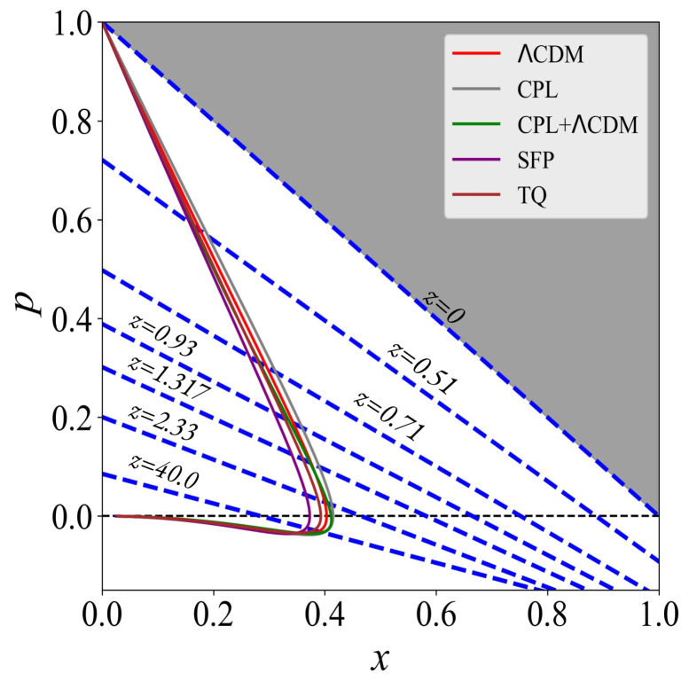
Figure 1: The cosmological evolution in the $(x,p)$ phase space for different models. The dotted straight lines correspond to the consistency condition Eq.( 3) for different redshifts (assuming a $\Lambda$CDM Universe). The intersection of the phase trajectories with these lines gives the value of $(x,p)$ at any particular redshift $z$.

Thus, to integrate this dynamical system and thereby determine the evolution history we need the function $E^{\prime}(z)$.

We will assume that, for a multi-component Universe it is possible to express

$$E(z)^{2}=\Omega_{m0}(1+z)^{3}+\Omega_{r0}(1+z)^{4}+\Omega_{\phi}f(z)$$ (6)

where, the dark matter and radiation components are treated independently from the unknown dark energy sector. The function $f(z)$ which imprints the dynamics of dark energy is usually obtained using the equation of state EoS parameter $w(z)=P_{DE}/\rho_{DE}$ for diverse dark energy models.

In terms the equation of state parameter $w(z)$, we have for a spatially flat cosmology

$${E}^{\prime}=\frac{3}{2}\left[\frac{E(1+w)}{(1+z)}-\frac{\Omega_{m0}w}{E}(1+z)^{2}+\frac{\Omega_{r0}(1+z)^{3}}{3E}\right.$$

$$\left.-\frac{\Omega_{r0}w(1+z)^{3}}{E}\right]$$ (7)

Ignoring $\Omega_{r0}$, the source term $F(x,p,z)$ can, thus be written as

$$F(x,p,z)=-\frac{2p}{1+z}-\frac{3}{2}\frac{\left(1+w\right)(x+p+pz)}{(1+z)^{2}}$$

$$+\frac{3}{2}\Omega_{m0}w(1+z)\left({x+p+pz}\right)^{3}$$ (8)

Thus, for a given dark energy model $w(z)$ and a set of cosmological parameters, the solution to the problem of finding the evolution history effectively reduces to solving a three dimensional autonomous system of non-linear differential equations

$$x^{\prime} =p$$ (9)

$${p}^{\prime} =F(x,p,z)$$

$$z^{\prime} =1$$

with initial conditions $(x_{o},p_{o},z_{o})=(0,1,0)$. The solution to this system of equations directly gives us $(x(z),p(z))$ which can be then used to find $D_{A}(z)$ and $H(z)$ using the consistency relation in Eq.(3). Fig.1 shows the cosmic expansion history in the $(x,p)$ phase space. The lines of consistency given by Eq.(3) are shown in the figure for some redshifts. The present epoch $(z=0)$ corresponds to the line that passes through $(0,1)$ and $(1,0)$ and all epochs with $z>0$ lie below it. The shaded gray region above this line corresponds to $z<0$. The intersection of the straight line corresponding to any redshift $z$ with the solution $(x(z),p(z))$ of the dynamical system in Eq.(9) gives the value of $(x,p)$ at that redshift. Regardless of the cosmological model, all phase trajectories must start at $(0,1)$ at $z=0$ and approach the origin $(0,0)$ as $z\rightarrow\infty$ which corresponds to the big bang. There is a redshift at which the phase trajectory intersects the $p=0$ line, which gives the maximum angular diameter distance. The difference between different cosmological models is maximal around this redshift in the $(x,p)$ plane. The phase trajectory can be obtained by adopting some model $w(z)$. In Fig.1 we have shown the cosmological evolution for the following models in phase space.

• The $\Lambda$CDM model ($w=-1$): For this widely popular model, we have adopted the cosmological parameters from PLANCK [95]

• The CPL model: In this model [96] $w_{\phi}$ is given by

  $$w_{\phi}=w_{o}+w_{a}\frac{z}{1+z}$$ (10)

  and provides a phenomenological parametrization to describe several features of dark energy using two parameters $(w_{o},w_{a})$. This model has been extensively used as the standard two parameter characterization of dynamical dark energy [97]. Further, a wide class of quintessence scalar field models can also effectively be mapped into the CPL parametrization [98]. As $z\rightarrow 0$, $w\rightarrow w_{o}$ and for the early Universe as $z\rightarrow\infty$, $w\rightarrow w_{o}+w_{a}$. This also means that the parameter $w_{a}$ can not take a very wide range of values in this model.

• The CPL-$\Lambda$CDM model: This is a cosmological model involving a negative cosmological constant (AdS vacua in the dark energy sector) along with a quintessence field ($\rho_{DE}=\Lambda+\rho_{\phi}$). The quintessence field is given a CPL parametrization ($w_{o},w_{a}$). The parameters of this model are adopted from [99].

• Scale Factor Parametrization: (SFP) In this model the scale factor is parametrized using $A,B$ in a way that

  $$H^{2}(z)=H_{0}^{2}\left[A(1+z)^{2/B}+(1-A)\right]$$

  In this model all the observables related to background evolution are constructed from the scale factor $a(t)$ only [100].

• Thawing Quintessence (TQ): Thawing models are characterized by flat potentials and the the field begins with $w\sim-1$ and increases only slightly to the present epoch. We adopt the equation of state from [101].

This is only a small sample of models and by no means exhaust the range of possible redhshift dependancy of $w(z)$. In this work, instead of assuming any specific model $w(z)$, we adopt a kinematic approach. We shall discuss this in the next section.

II.2 The semi-cosmographic reconstruction

We adopt two kinematic cosmographic descriptions of background evolution where the Luminosity distance can be expressed as a Padé rational fraction expansion. Firstly, we consider the standard Padé approximants as ratios of polynomials in the redshift $z$ [82, 78, 71, 102, 72] and assume that

$${\rm\bf Case\leavevmode\nobreak\ I}:\leavevmode\nobreak\ \leavevmode\nobreak\ \leavevmode\nobreak\ \leavevmode\nobreak\ \leavevmode\nobreak\ \leavevmode\nobreak\ D_{L}^{\cal{P}}(z)=\frac{c}{H_{0}}{\mathcal{P}}_{(m,n)}(z)$$ (11)

where $\mathcal{P}_{(m,n)}$ is the Padé approximant $(m,n)$ given by

$${\cal{P}}_{(m,n)}(z)=\frac{a_{1}z+a_{2}z^{2}+\dots+a_{m}z^{m}}{1+b_{1}z+b_{2}z^{2}+\dots+b_{n}z^{n}}.$$ (12)

The expansion coefficients can be related to kinematic quantities like $H_{0}$, $q_{0}$, $j_{0}$, $s_{0}$ $l_{0}...$ by comparing this Padé expansion with the Taylor expansion [67, 75, 103, 82, 102, 72, 77, 78, 59, 71]. We don’t make any such connections ab initio and treat the Padé expansion coefficients $(a_{m},b_{n})$ themselves as the parameters of interest.

Moreover, we note that connections of the Padé parameters with the kinematic quantities become more complicated in the second description that we adopt. In this case, we assume that the Padé expansion is in terms of the variable $\xi=\sqrt{1+z}$ [90].

$${\rm\bf Case\leavevmode\nobreak\ II}:\leavevmode\nobreak\ \leavevmode\nobreak\ \leavevmode\nobreak\ \leavevmode\nobreak\ \leavevmode\nobreak\ \leavevmode\nobreak\ D_{L}^{\cal{R}}(z)=\frac{c}{H_{0}}{\cal{R}}(\sqrt{1+z})$$ (13)

where the function ${\cal{R}}(\xi)$ is given by

$${\cal{R}}(\xi)=2\left[\frac{\xi^{4}-\alpha\xi^{3}-(1-\alpha)\xi^{2}}{\beta\xi^{2}+\gamma\xi+2-\alpha-\beta-\gamma}\right]$$ (14)

This choice of the Padé approximant is motivated by the fact that $D_{L}$ and $H$ obtained from it has the desired asymptotic behaviour [90].

For each of these cosmographic descriptions (Case I and Case II), the corresponding approximants for angular diameter distance $D_{A}^{{\cal P}/{\cal R}}(z)$ and Hubble parameter $H^{{\cal P}/{\cal R}}(z)$ for a spatially flat cosmology are given by

$$D_{A}^{{\cal P}/{\cal R}}(z)=\frac{D_{L}^{{\cal P}/{\cal R}}}{(1+z)^{2}}\leavevmode\nobreak\ \leavevmode\nobreak\ \&\leavevmode\nobreak\ \leavevmode\nobreak\ H^{{\cal P}/{\cal R}}(z)=c\left[\frac{d}{dz}\frac{D_{L}^{{\cal P}/{\cal R}}}{(1+z)}\right]^{-1}$$ (15)

In the standard cosmographic approach, $D_{L}^{{\cal P}/{\cal R}}(z)$, $D_{A}^{{\cal P}/{\cal R}}(z)$ and $H^{{\cal P}/{\cal R}}(z)$ are fitted with observational data to obtain constraints on kinematic parameters $(a_{1},a_{2}\dots,a_{m},b_{1},b_{2}\dots,b_{n},H_{0})$ or $(\alpha,\beta,\gamma,H_{0})$ depending on which case one adopts. This does not allow for easy direct constraints on $\Omega_{m0}$ or any other density parameters, unless the kinematic quantities are expressed in terms of these parameters using the Taylor-Padé connection. Instead of trying to connect the Taylor expansion with the Padé expansion, we propose a semi-cosmographic approach to constrain the expansion history by defining

$$w^{[\Omega_{m},{\cal P}/{\cal R}]}\left(z\right)=\frac{\frac{2}{3}\left(1+z\right)\frac{d}{dz}{\rm{ln}}H^{{\cal P}/{\cal R}}-1}{1-\left(\frac{H_{0}}{H^{{\cal P}/{\cal R}}\left(z\right)}\right)^{2}\Omega_{m0}\left(1+z\right)^{3}}.$$ (16)

This semi-cosmographic equation of state parameter $w^{[\Omega_{m},{\cal P}/{\cal R}]}\left(z\right)$, now additionally depends on $\Omega_{m0}$ along with the kinematic parameters $(H_{0},a_{1},a_{2}\dots,a_{m},b_{1},b_{2}\dots,b_{n})$ of ${\cal P}_{(m,n)}(z)$ or $(H_{0},\alpha,\beta,\gamma)$ of ${\cal R}(z)$. It seams together kinematic information in ${\cal P}(z)$ or ${\cal R}(z)$ with the dynamical information imprinted in $E(z)$. Using this semi-cosmographic equation of state $w^{[\Omega_{m},{\cal P}/{\cal R}]}$ in Eq.(8), the autonomous system in Eq. (9) can be solved numerically for $x(z)$ and $p(z)$. This gives us a new set of quantities $(D_{A}(z),D_{L}(z),H(z))$ for scenarios $\bf I$ and $\bf II$:

$$D_{A}=\frac{cx}{H_{0}},\leavevmode\nobreak\ D_{L}=\frac{c(1+z)^{2}x}{H_{0}},\leavevmode\nobreak\ H=\frac{H_{0}}{x+p+pz}$$ (17)

Thus, for each of the starting cosmographic scenarios, we have two sets of expressions for the distances and Hubble expansion rate: the original cosmographic $(D_{L}^{{\cal P}/{\cal R}}(z),D_{A}^{{\cal P}/{\cal R}}(z),H^{{\cal P}/{\cal R}}(z))$ and $(D_{L}(z),D_{A}(z),H(z))$. The first set has no pre-assumptions about cosmological dynamics, whereas the second set is based on the specific form of $E(z)$ in Eq.(6) and the equation of state $w^{[\Omega_{m},{\cal P}/{\cal R}]}$ in Eq.(16). For internal consistency, observational data must constrain the parameter space simultaneously for both sets of functions for the same physical quantities. Given the distinct nature of the two forms of functions, the posterior distribution of the parameters for joint estimation using both together tends to give a bimodal distribution for $\Omega_{m0}$. To avoid this issue, we use the posterior distribution on the parameters $(H_{0},a_{1},a_{2},\dots,b_{1},b_{2}\dots)$ or $(H_{0},\alpha,\beta,\gamma)$ obtained by directly fitting data with $(D_{L}^{{\cal P}/{\cal R}},D_{A}^{{\cal P}/{\cal R}},H^{{\cal P}/{\cal R}})$ as priors for fitting the same data with $(D_{L},D_{A},H)$. For this second fitting based on the solution of the autonomous system with $w^{[\Omega_{m},{\cal P}/{\cal R}]}$, we additionally assume flat priors for $\Omega_{m0}$. The fit using $(D_{L}^{{\cal P}/{\cal R}},D_{A}^{{\cal P}/{\cal R}},H^{{\cal P}/{\cal R}})$ limits the vast parameter space of the kinematic parameters, while the subsequent fit using $(D_{L},D_{A},H)$, shifts the parameters for consistency with dynamical information now incorporated in the modeling.

Using cosmological data on distances and Hubble parameter and adopting this two step fitting process, the phase-space orbit can be reconstructed. Apart from that, the best fit values of the parameters and their respective errors are used to reconstruct some important diagnostic probes of background cosmology. We apply our fitting method to reconstruct the following quantities which are related to each other.

• The dark energy EoS $w(z)$: This is the most commonly used quantifier of dark energy dynamics. For accelerated expansion we require that dark energy violate the strong energy condition with $w(z)<-1/3$. If the acceleration is driven by the cosmological constant then $w=-1$ and any departure from this implies that dark energy is dynamic. For scalar field dark energy one may have the freezing models, where $w(z)$ does not evolve significantly and remains close to $-1$ throughout the cosmic expansion. In case of thawing models $w(z)$ starts close to $-1$ and evolves toward less negative values as the universe expands.

• The ${\cal{O}}m$ diagnostic: The ${\cal{O}}m$ diagnostic proposed in [104], is an useful quantifier of evolving dark energy. This is defined as

  $${\mathcal{O}}m(z)=\frac{E(z)^{2}-1}{\left(1+z\right)^{3}-1}$$ (18)

  Except for $z=0$, where it diverges, this quantity measures any departure from the $\Lambda$CDM model since its value is a constant $\Omega_{m0}$ the $\Lambda$CDM model. Further, ${\mathcal{O}}m(z)>\Omega_{m0}$ in Quintessence and ${\mathcal{O}}m(z)<\Omega_{m0}$ in Phantom dark energy models.

• Evolution of DE $f(z)$: We define dark energy evolution using

  $$f(z)=\frac{E(z)^{2}-\Omega_{m0}\left(1+z\right)^{3}}{1-\Omega_{m0}}$$ (19)

  Like ${\mathcal{O}}m(z)$ and $w(z)$, this quantity imprints the evolution of the dark energy density. For the $\Lambda$CDM model, $f(z)=1$. Thus, any departure from unity at low redshifts indicates dynamical dark energy.

• The AP distortion parameter $F(z)$: The Alcock–Paczynski effect [94] is used to constrain cosmological models by comparing the observed tangential and radial size of objects which are otherwise assumed to be isotropic. If $\Delta z$ and $\Delta\theta$ are the radial and tangential extents of the object then the quantity of interest is $F(z)=\Delta z/\Delta\theta$. This can be written as

  $$F(z)=\frac{(1+z)D_{A}(z)H(z)}{c}$$ (20)

  The AP test aims to measure the departure of this quantity from its value in a fiducial cosmology.

• The BAO distance measure $D_{V}(z)$: Galaxy surveys imprint both the transverse and the radial BAO peaks. It is however difficult to probe large radial distances leading to small survey depths. Further, large shot noise degrades the SNR making it very difficult to independently measure $D_{A}(z)$ and $H(z)$. Typically, the combination $D_{V}(z)$ is measured instead in galaxy redshift surveys [5, 105] given by

  $$D_{V}(z)=\left[(1+z)^{2}D_{A}(z)^{2}\frac{cz}{H(z)}\right]^{\frac{1}{3}}$$ (21)

  This quantity is often used in BAO analysis when high SNR anisotropic data is not available.

III Observational Aspects and Data

In this section, we discuss the cosmological data used from various cosmological probes for our analysis. We have considered two main data sources. Since our initial Padé expansion is for the Luminosity distance, we consider distance measurements using SNIa apparent magnitude. We also consider BAO data which gives the $(D_{A}(z),H(z))$ information for our phase space analysis.

III.1 BAO Data

We use the BAO data on $\tilde{D}_{M}$ and $\tilde{D}_{H}$ defined as

$$\tilde{D}_{M}=\frac{c}{r_{d}}\int_{0}^{z}\frac{dz^{\prime}}{H(z^{\prime})}\leavevmode\nobreak\ \leavevmode\nobreak\ \leavevmode\nobreak\ \&\leavevmode\nobreak\ \leavevmode\nobreak\ \leavevmode\nobreak\ \leavevmode\nobreak\ \tilde{D}_{H}=\frac{c}{Hr_{d}}$$ (22)

where $r_{d}$ is the sound horizon at the drag epoch. In our analysis we have adopted $r_{d}=146.995\pm 0.264\leavevmode\nobreak\ {\rm Mpc}$, from CMBR constraints [106, 57]. The tracers included in the DESI BAO data are luminous red galaxy (LRG), emission line galaxies (ELG) and the Lyman-$\alpha$ forest (Ly-$\alpha$QSO) in a redshift range $0.1\leq z\leq 4.2$. We adopt the anisotropic BAO data from DESI DR1 for LRG, ELG and Ly-$\alpha$ tracers at $5$ redshifts $z_{eff}=0.51,0.706,0.93,1.32$ and $2.33$ respectively. The mean, variance and correlation information is adopted from [107]. For two other redshifts $z_{eff}=0.295$ and $1.491$ we have taken the isotropic BAO data on $D_{V}$ [107].

Further, we have taken measured anisotropic data on $D_{A}(z)$ and $H(z)$ from eBOSS DR12 [108] and eBOSS DR16 [109, 110, 111] at redshifts $0.38,0.51,0.698,1.48,2.334$. All covariance matrices are suitably transformed to relevant quantities $(x,p)$ using the Jacobian matrices for the corresponding transformation.

III.2 SNIa Data

The measurement of the Luminosity distance using Supernova Type Ia (SNIa) has been a crucial cosmological probe and amongst the earliest to indicate cosmic acceleration [112]. The Pantheon+ sample consists of apparent magnitude data for 1701 SNIa light curves in the redshift range $0.00122\leq z\leq 2.26137$ [93, 113]. To avoid the issue of strong peculiar velocity dependence at low redshifts [113] we have not considered $111$ light curves in the range $z<0.01$. We have adopted the data and its full statistical and systematic covariance from https://github.com/PantheonPlusSH0ES/DataRelease.

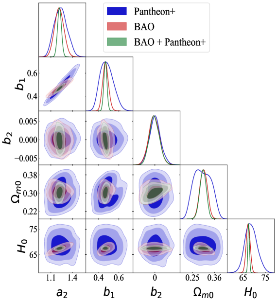
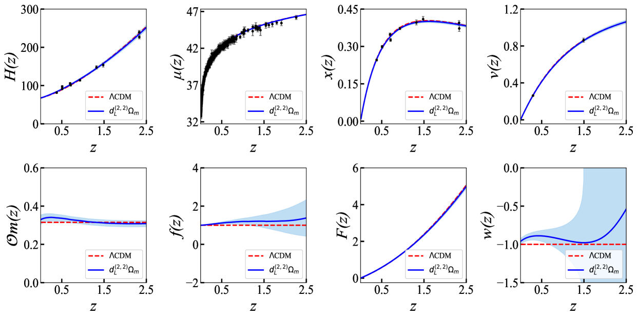
Figure 2: Marginalized posterior distribution of the set of semi-cosmographic parameters ($H_{0},\Omega_{m},a_{2},b_{1},b_{2}$) and the corresponding 2D confidence contours obtained from the MCMC analysis starting with $D_{L}^{\mathcal{P}}$. The confidence contours correspond to data being fitted with BAO(DESI+eBOSS), Pantheon+, and joint BAO+Pantheon, respectively. The panel on the right shows the reconstruction of some diagnostics of background cosmology and their $1\sigma$ errors from the joint BAO+Pantheon analysis. The corresponding quantities for the $\Lambda$CDM model is superposed for comparison.

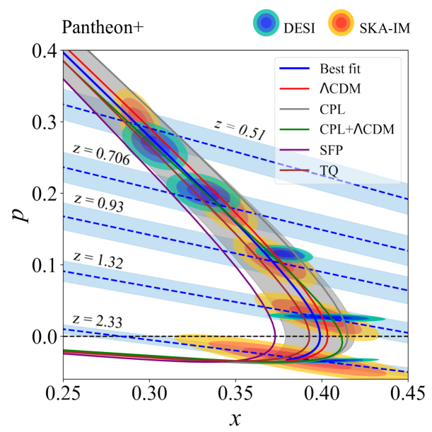
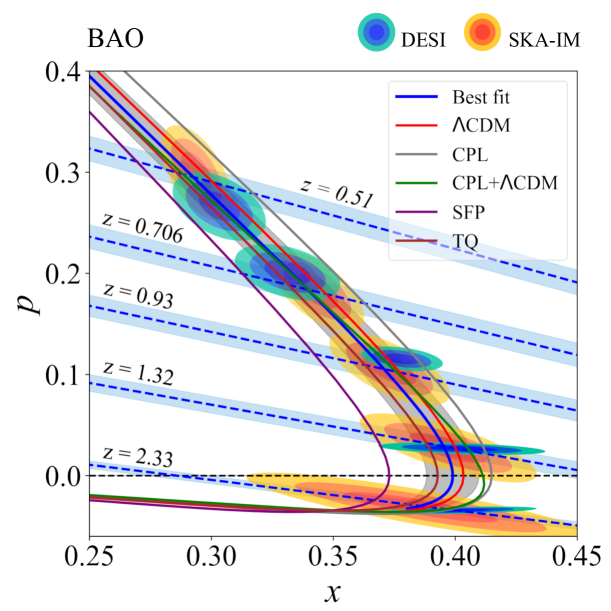
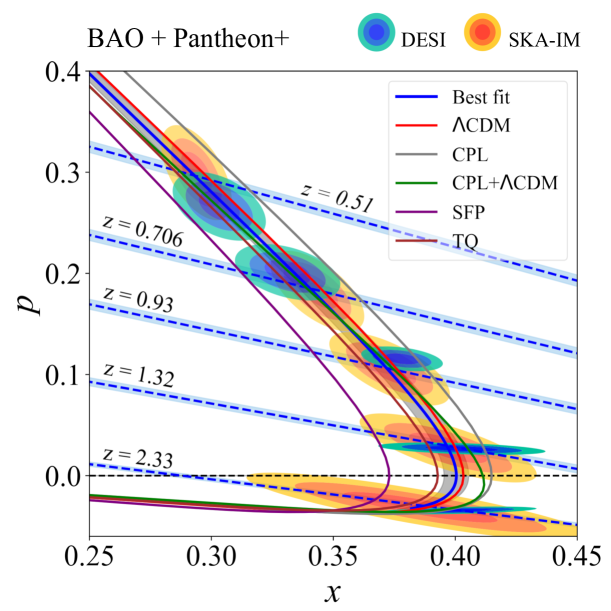
Figure 3: The reconstructed phase space trajectory $(x(z),p(z))$ with $1\sigma$ error for cosmography starting with $D_{L}^{P}(z)$. Several dark energy models are also shown for comparison. The left-most figure corresponds to a reconstruction with Pantheon+ data, the middle figure corresponds to a fit with BAO(DESI+eBOSS) data and the right-most figure corresponds to a joint analysis. The actual DESI error contours at 5 redshifts and the projected error contours for a 21-cm intensity mapping experiment at observing frequencies corresponding to the same redshifts are shown. We also show the consistency lines corresponding to the same redshifts with its error (originating from $H(z)$).

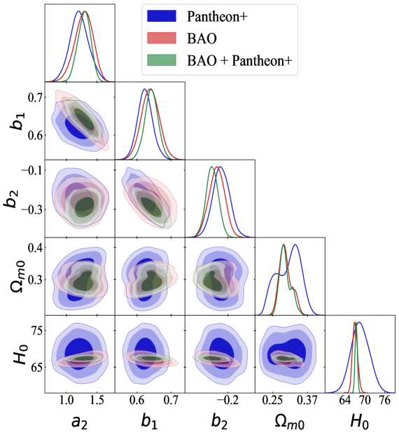
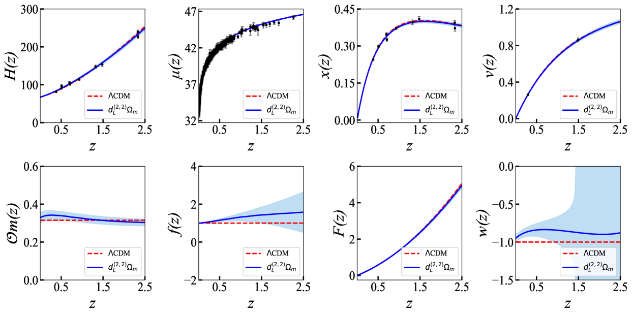
Figure 4: Marginalized posterior distribution of the set of semi-cosmographic parameters ($H_{0},\Omega_{m},\alpha,\beta,\gamma$) and the corresponding 2D confidence contours obtained from the MCMC analysis starting with $D_{L}^{\mathcal{R}}$. The confidence contours correspond to data being fitted with BAO(DESI+eBOSS), Pantheon+, and joint BAO+Pantheon, respectively. The panel on the right shows the reconstruction of some diagnostics of background cosmology and their $1\sigma$ errors from the joint BAO+Pantheon analysis. The corresponding quantities for the $\Lambda$CDM model is superposed for comparison.

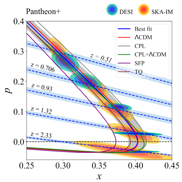
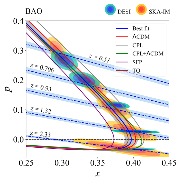
Figure 5: The reconstructed phase space trajectory $(x(z),p(z))$ with $1\sigma$ error for cosmography starting with $D_{L}^{R}(z)$. Several dark energy models are also shown for comparison. The left-most figure corresponds to a reconstruction with Pantheon+ data, the middle figure corresponds to a fit with BAO(DESI+eBOSS) data and the right-most figure corresponds to a joint analysis. The actual DESI error contours at 5 redshifts and the projected error contours for a 21-cm intensity mapping experiment at observing frequencies corresponding to the same redshifts are shown. We also show the consistency lines corresponding to the same redshifts with its error (originating from $H(z)$).

Model $D_{L}^{\cal P}$	$H_{0}$	$\leavevmode\nobreak\ \leavevmode\nobreak\ \leavevmode\nobreak\ \leavevmode\nobreak\ \Omega_{m0}$	$\leavevmode\nobreak\ \leavevmode\nobreak\ \leavevmode\nobreak\ \leavevmode\nobreak\ \leavevmode\nobreak\ \leavevmode\nobreak\ a_{2}$	$\leavevmode\nobreak\ \leavevmode\nobreak\ \leavevmode\nobreak\ \leavevmode\nobreak\ \leavevmode\nobreak\ \leavevmode\nobreak\ b_{1}$	$b_{2}$	$\chi^{2}_{\rm red}$	$AIC$
DESI+eBOSS	$67.24^{+0.90}_{-0.90}$	$0.305^{+0.019}_{-0.019}$	$1.216^{+0.065}_{-0.065}$	$0.469^{+0.029}_{-0.029}$	$-0.0002^{+0.0016}_{-0.0016}$	1.005	37.14
Pantheon+	$68.6^{+2.5}_{-2.9}$	$0.300^{+0.041}_{-0.041}$	$1.236^{+0.082}_{-0.100}$	$0.480^{+0.056}_{-0.075}$	$\leavevmode\nobreak\ \leavevmode\nobreak\ 0.0001^{+0.0018}_{-0.0018}$	0.886	1414.11
BAO+Pantheon+	$67.47^{+0.36}_{-0.36}$	$0.302^{+0.016}_{-0.016}$	$1.220^{+0.027}_{-0.027}$	$0.466^{+0.016}_{-0.016}$	$-0.0001^{+0.0015}_{-0.0015}$	0.885	1440.31
Model $D_{L}^{\cal R}$	$H_{0}$	$\leavevmode\nobreak\ \leavevmode\nobreak\ \leavevmode\nobreak\ \leavevmode\nobreak\ \Omega_{m0}$	$\leavevmode\nobreak\ \leavevmode\nobreak\ \leavevmode\nobreak\ \leavevmode\nobreak\ \leavevmode\nobreak\ \leavevmode\nobreak\ \alpha$	$\leavevmode\nobreak\ \leavevmode\nobreak\ \leavevmode\nobreak\ \leavevmode\nobreak\ \leavevmode\nobreak\ \leavevmode\nobreak\ \beta$	$\leavevmode\nobreak\ \leavevmode\nobreak\ \leavevmode\nobreak\ \leavevmode\nobreak\ \leavevmode\nobreak\ \leavevmode\nobreak\ \leavevmode\nobreak\ \leavevmode\nobreak\ \leavevmode\nobreak\ \gamma$	$\chi^{2}_{\rm red}$	$AIC$
DESI+eBOSS	$67.05^{+0.69}_{-0.84}$	$0.295^{+0.015}_{-0.027}$	$1.28^{+0.16}_{-0.13}$	$0.639^{+0.026}_{-0.026}$	$-0.263^{+0.044}_{-0.044}$	$\leavevmode\nobreak\ \leavevmode\nobreak\ \leavevmode\nobreak\ \leavevmode\nobreak\ \leavevmode\nobreak\ \leavevmode\nobreak\ \leavevmode\nobreak\ 1.007$	$37.19$
Pantheon+	$68.6^{+2.8}_{-2.8}$	$0.304^{+0.041}_{-0.041}$	$1.21^{+0.16}_{-0.16}$	$0.624^{+0.022}_{-0.022}$	$-0.238^{+0.048}_{-0.048}$	$0.886$	$1414.31$
BAO+Pantheon+	$67.40^{+0.035}_{-0.035}$	$0.294^{+0.020}_{-0.020}$	$1.29^{+0.11}_{-0.098}$	$0.642^{+0.019}_{-0.019}$	$-0.298^{+0.035}_{-0.035}$	$0.885$	$1440.54$

Table 1: The parameter values obtained in the MCMC analysis are tabulated along with the $1\sigma$ uncertainty.

III.3 BAO imprint on the 21-cm Intensity Mapping

Traditional Baryon Acoustic Oscillation (BAO) surveys, such as DESI and BOSS, rely on the distribution of galaxies and quasars, which are typically constrained to redshifts $(z\leq 3)$. In contrast, 21 cm Intensity Mapping (IM) probes BAO deep into the reionization era $(z>6)$, extending BAO studies further into cosmic history [114]. IM offers significant advantages over galaxy surveys due to its ability to cover larger volumes at higher redshifts, thereby improving efficiency [115, 116]. Several radio telescopes such as HIRAX[117], CHIME[118], and SKA[119, 120] are aiming to detect BAO signal using 21cm IM in near future. The potentially large survey volumes for 21-cm intensity mapping experiments makes it possible to measure radial and transverse BAO features with high SNR. In the absence of actual data, we model the observed data using error projections from a SKA1-Mid like radio interferometer.

In the post-reionization universe $(z\leq 6)$, DLAs are the dominant reservoirs of HI, containing $\approx 80\%$ of the neutral hydrogen at $z<4$ [121] with HI column density greater than $2\times 10^{20}$atoms/$\rm cm^{2}$ [122, 123, 124]. The post EoR power spectrum $P_{21}$ of the 21-cm excess brightness temperature field can be modeled in the linear regime as [125, 116, 115, 126]

$$P_{21}(k,z,\mu)=C^{2}_{T}(z)\leavevmode\nobreak\ {(1+\beta_{T}\mu^{2})}^{2}\leavevmode\nobreak\ P_{m}(k,z)$$ (23)

where $\mu={\bf{k}}\cdot{\bf{\hat{n}}}$ and $\beta_{T}=f_{g}(z)/b_{T}$, where $f_{g}(z)$ is the logarithmic growth rate of matter fluctuations, $b_{T}$ being the HI bias and $P_{m}$ is the dark matter power spectrum [92]. The redshift space distortion (RSD) factor $1+\beta_{T}\mu^{2}$ arises due to the peculiar velocity of the HI clouds [127, 115, 128]. The overall amplitude ${\mathcal{C}}_{T}$ is the average HI brightness temperature, given by,

$${\mathcal{C}}_{T}=4.0\,{\rm{mK}}\,b_{T}\,{\bar{x}_{\rm HI}}(1+z)^{2}\left(\frac{\Omega_{b0}h^{2}}{0.02}\right)\left(\frac{0.7}{h}\right)\left(\frac{H_{0}}{H(z)}\right)$$ (24)

The mean HI fraction $\bar{x}_{\rm HI}$ and bias $b_{T}$ that completely model post-EoR 21cm power spectrum are largely uncertain. However, in the post-EoR epoch $\bar{x}_{HI}$ does not evolve much [122, 124]. Simulation studies show that the bias is scale dependent on small scales below the Jean’s length [129]. However, on large scales the bias is expected to be scale-independent [130, 131, 132]. In our analysis we kept the fiducial value of $\bar{x}_{HI}=2.45\times 10^{-2}$ [124] and consider the fitting of bias from [131]. The BAO manifests itself as a series of oscillations in the linear matter power spectrum. The Baryonic feature is seen clearly if we subtract the cold dark matter contribution from the total power spectrum: $P_{b}(k)=P(k)-P_{c}(k)$. The BAO power spectrum can be modeled as [133, 29]

$$P_{b}(k^{\prime})=A\frac{\sin x}{x}e^{-(k^{\prime}\Sigma_{s})^{1.4}}e^{-k^{\prime 2}\sum_{nl}^{2}/2}$$ (25)

where $A$ is a normalization constant, $\Sigma_{s}=1/k_{silk}$ and $\sum_{s}=1/k_{nl}$ denotes the inverse scale of ‘Silk-damping’ and ‘non-linearity’ respectively. In our analysis we have used $k_{nl}=(3.07h^{-1}$Mpc$)^{-1}$and $k_{silk}=(8.38h^{-1}$Mpc$)^{-1}$ from [29] and $x=\sqrt{k^{2}(1-\mu^{2})s_{\perp}^{2}+k^{2}\mu^{2}s_{\parallel}^{2}}$, where $s_{\perp}$ and $s_{\parallel}$ are the transverse and radial sound horizon scales, respectively. The changes in $D_{A}(z)$ and $H(z)$ are reflected in the variations of $s_{\perp}$ and $s_{\parallel}$. The fractional errors in these quantities correspond to the uncertainties in $D_{A}/s$ and $sH$, where $s=r_{d}$ represents the true physical value of the sound horizon.

To quantify these errors, we define the parameters, $p_{1}=\ln(s^{-1}_{\perp})$ and $p_{2}=\ln(s_{\parallel})$ and use them in our analysis to derive the Cramer-Rao bounds: $\sqrt{F^{-1}_{ii}}=\delta D_{A}/D_{A}$ and $\sqrt{F^{-1}_{jj}}=\delta H/H$ respectively, where $F^{-1}_{ii}$ represents the Fisher matrix elements and is given by [134]

$$F_{ij}=\int dk^{\prime}\leavevmode\nobreak\ \int_{0}^{1}d\mu\leavevmode\nobreak\ \frac{C^{2}_{T}}{\delta P^{2}_{21}}\left[1+\beta_{T}\mu^{2}\right]^{2}\left(\cos x-\frac{\sin x}{x}\right)^{2}$$

$$\times f_{i}(\mu)f_{j}(\mu)A^{2}e^{-2(k^{\prime}\sum_{s})^{1.4}}e^{-k^{\prime 2}\sum_{nl}^{2}}$$

where $f_{1}=\mu^{2}-1$ and $f_{2}=\mu^{2}$. The term $\delta P_{21}^{2}$ is the variance of 21cm experiment. We adopt the theoretical expected noise for a radio interferometric experiment from [135, 136, 137, 138]. For a radio interferometric observational frequency $\nu=1420/(1+z)$MHz or wavelength $\lambda=0.21(1+z)$m, we have

$$\delta P_{\rm HI}(k,\mu,z)=\frac{P_{\rm HI}(k,\mu,z)+N_{T}(k,\mu,z)}{\sqrt{N_{c}}}$$ (26)

where

$$N_{T}=\frac{\lambda^{2}T_{sys}^{2}r^{2}dr/d\nu}{A_{e}t_{\mathbf{k}}}$$ (27)

Here $A_{e}$ is the effective area of the individual antenna dish, $T_{sys}$ is the system temperature, $r$ is the comoving distance to the source and

$$t_{\mathbf{k}}=T_{o}N_{ant}\left(N_{ant}-1\right)A_{e}\rho/2\lambda^{2}$$ (28)

is the fraction of the total observation time $T_{o}$ spent on each mode. We have considered a radio-array with $N_{ant}$ antennae spread out in a plane, such that the total number of visibility pairs $N_{ant}(N_{ant}-1)/2$ are distributed over different baselines according to a normalized baseline distribution function $\rho(k_{\perp},\nu)$.

$$\rho_{b}({\bf{k_{\perp}}}=2\pi{\bf{u}}/r)=c\int d^{2}{{\bf r}}\rho_{ant}({\bf r})\rho_{ant}({\bf r}-\lambda{\bf{u}})$$ (29)

Where $c$ is fixed by normalization of $\rho_{b}({\bf{u}})$ and $\rho_{ant}$ is the distribution of antennae. We assume $\rho(r)\sim 1/r^{2}$.

The noise is suppressed by a factor $\sqrt{N_{c}}$ where $N_{c}$ is the number of modes in a given survey volume. We have

$$N_{c}=2\pi k^{2}\Delta k\Delta\mu r^{2}(dr/d\nu)B\lambda^{2}/A_{e}(2\pi)^{3}$$ (30)

The noise estimates are based on a futuristic SKA1-Mid like intensity mapping experiment. We consider an interferometer with $250$ dish antennae each of diameter $15$m For the SKA-Mid frequency band 1 and 2 ($400-950$MHz) the assumed frequency bandwidth is $32$MHz. We assume $500$ hours of observation per pointing and consider multiple pointings for a full sky observation. We consider the spherically averaged power spectrum which is binned in logarithmically spaced bins in $k$, with $dk/k=1/6$. The minimum wavenumber is set to $k_{\rm min}=0.005$ h Mpc^-1 to ensure the validity of Newtonian perturbation theory, while the maximum wavenumber is limited to $k_{\rm max}=0.2h$ Mpc^-1 to remain within the linear regime. For sufficiently long observations, instrumental noise becomes negligible, and the signal-to-noise ratio (SNR) is dominated by cosmic variance. In this regime, the covariance of the measurement can only be further reduced by a factor of $1/\sqrt{N_{p}}$ where $N_{p}$ as the number of independent pointings. We also note that small $k_{\parallel}$, are plagued by foreground contaminants. This corresponds to the large $\Delta_{\nu}$ over which the foregrounds are correlated. This required us to remove these modes.

IV Results and Discussion:

We first discuss our results for the scenario described as $\bf Case\leavevmode\nobreak\ I$. We consider the Padé approximated luminosity distance of order $\left(2,2\right)$ given by Eq.(11). We choose $a_{1}=1$ so that we have

$$D_{L}^{\cal P}(z)=\frac{c}{H_{0}}\frac{z+a_{2}z^{2}}{1+b_{1}z+b_{2}z^{2}}$$ (31)

This kinematic expansion and $D_{A}^{\cal P}$ and $H^{\cal P}$ obtained from Eq.(31) using Eq.(15) has parameters $(H_{0},a_{2},b_{1},b_{2})$. We obtain the semi-cosmographic equation of state using Eq.(16) which is then used to solve the dynamical system in Eq.(9) to obtain a new set $(D_{A},H)$. This new set, now additionally depend on the parameter $\Omega_{m0}$. Fig.(2) shows the results for fitting $(D_{L},D_{A},H)$ with BAO data from DESI and eBOSS, Pantheon+ and joint analysis with BAO+Pantheon. The posterior distribution of fitting the same data $D_{A}^{\cal P}$ and $H^{\cal P}$ are used as priors. The parameter estimation is done using MCMC (emcee code [139]). The best fit values of the parameters $(H_{0},\Omega_{m0},a_{1},b_{1},b_{2})$ and the $1\sigma$ errors are summarized in Table-1. The value of $\chi^{2}_{red}\sim 1$, indicates that it is a good fit.

The panel in Figure (2) shows the best-fit reconstruction of ($H(z)$, $\mu(z)$, $x=H_{0}D_{A}(z)/c$, $v=D_{V}H_{0}/c$, ${\cal{O}}m(z)$, $f(z)$, $F(z)$, $w(z)$) with the $1\sigma$ errors obtained from the MCMC using joint analysis with BAO DESI + eBOSS and Pantheon+ data. The corresponding quantities for the $\Lambda$CDM model (with PLANCK parameters) are also shown in the same figures for comparison. All the diagnostics seem to indicate that at $1\sigma$ the cosmographic model can not be distinguished from the $\Lambda$CDM model specially at higher redshifts. The best fit for ${\cal{O}}m(z)>\Omega_{m0}$ seems to weakly favour quintessence models. The worst constraint seems to be on $f(z)$ and the related equation of state parameter $w(z)$ which have large errors. $w(z)$ also seems to have an unphysical divergence at large redshifts. This is one of the key drawbacks of the cosmographic aproach. The qualititative features of the reconstructed diagnostics have similar behaviour as reported in literature for other model-independent/cosmographic approaches.

Fig.(3) shows the reconstructed phase space trajectory using BAO (DESI+ eBOSS), Pantheon+ and joint (BAO+Pantheon) data respectively for the semi-cosmographic analysis on $D_{L}^{\cal P}$. The best fit phase trajectory and its $1\sigma$ error is shown. The lines of consistency are shown at the 5 redshifts corresponding to the DESI BAO data. The $1\sigma$ errors on these lines correspond to the uncertainties in the $p-$intercept which are related to the uncertainties in the reconstructed $H(z)$ at the specific $z$. The intersections of the 1$\sigma$ band around the best fit trajectory with the bands around the lines of consistency gives the region of uncertainty of $(x,p)$ at a given redshift. We also show the phase space evolution for some cosmological models discussed in the earlier section. We find that all these models are consistent with the best-fit result and indistinguishable within 1$\sigma$ for the analysis with Pantheon+ data. With the inclusion of BAO(DESI + eBOSS) data, we find that the best-fit cosmographic model is at a 1$\sigma$ tension with the CPL and TQ model.

The actual DESI DR1 data (transformed to the new variables) at the 5 redshifts are superposed on the reconstructed phase-space. At redshifts $0.51,0.706$ and $0.93$ the DESI results are about $\sim 1.6\sigma$ tension with the results of the reconstruction from the joint analysis. We also show the projected 21-cm error contours at the same redshifts for a 21-cm intensity mapping experiment described in the last section. We find that at low redshifts the 21-cm projections are competitive with the BAO DR1 results for an idealized (perfect foreground cleaning) intensity mapping experiment.

Model $D_{L}^{\cal P}$	$q_{0}$	${j_{0}}$	$s_{0}$
DESI+eBOSS	$-0.518^{+0.077}_{-0.077}$	$1.61^{+0.42}_{-0.65}$	$3.2^{+1.1}_{-2.2}$
Pantheon+	$-0.532^{+0.055}_{-0.066}$	$1.71^{+0.59}_{-0.70}$	$3.6^{+1.2}_{-2.6}$
BAO+Pantheon+	$-0.528^{+0.032}_{-0.032}$	$1.59^{+0.23}_{-0.26}$	$3.06^{+0.65}_{-0.86}$

Table 2: The constraints on kinematic quantities with $1\sigma$ uncertainty for a Padé cosmography with $D_{L}^{\cal P}$.

In our analysis, we have made no assumption about the connection between a Padé approximation and Taylor series expansion. However, for the form of $D_{L}^{\cal P}(z)$ chosen by us, such a comparison is possible and the parameters $a_{2}$, $b_{1}$ and $b_{2}$ can be expressed in terms of the kinematic quantities $q_{0}$, $j_{0}$ and $s_{0}$. Using the relationship from [71, 84], we obtain the constraints on these kinematic quantities. The table 2 summarizes the constraints on $(q_{0},j_{0},s_{0})$, if these parameters were used in $D_{L}^{{\cal P}}$ instead of $(a_{2},b_{1},b_{2})$. The best fit values of these kinematic parameters are consistent with the findings in other cosmographic methods [84].

We shall now discuss the scenario described as $\bf Case\leavevmode\nobreak\ II$. Here we have the Padé approximated luminosity distance in the variable $(1+z)^{1/2}$ instead of $z$ given by Eq.(13). For this model $H(z)\rightarrow H_{0}$ as $z\rightarrow 0$ and $H(z)\propto(1+z)^{3/2}$ for $z>>1$. We first fit $D_{L}^{\cal R}(z)$ and $D_{A}^{\cal R}$ and $H^{\cal R}$ using parameters $(H_{0},\alpha,\beta,\gamma)$ with data using flat priors. The posteriors from these fits are then used as priors for fitting the semi-cosmographic $D_{L}(z)$, $H(z)$ and $D_{A}(z)$ obtained by solving Eq.(9) using $w^{[\Omega_{m},\cal R]}(z)$. We take flat priors for $\Omega_{m0}$ as before.

The estimated parameters and their $1\sigma$ errors are given in table 1. The constraints on $H_{0}$ and $\Omega_{m0}$ are comparable to the ones obtained using $D_{L}^{P}(z)$.

The Fig.(4) shows the results for fitting $(D_{A},H,D_{L})$ with BAO data (DESI and eBOSS), SnIa data from Pantheon+ and joint analysis with BAO+Pantheon. The reduced $\chi^{2}\sim 1$ implying that the fit is good.

The panel in Fig.(4) shows the best-fit reconstruction of ($H(z)$, $\mu(z)$, $x=H_{0}D_{A}(z)/c$, $v=D_{V}H_{0}/c$, ${\cal{O}}m(z)$, $f(z)$, $F(z)$, $w(z)$) with the $1\sigma$ errors obtained from joint analysis with BAO (DESI + eBOSS) and Pantheon+ data. The corresponding quantities for the $\Lambda$CDM model (with PLANCK parameters) are also shown in the same figures for comparison. Here too, all the diagnostics show that the semi-cosmographic model $\cal R$ can’t be distinguished from the $\Lambda$CDM model. At low redshifts the departure is $\sim 1\sigma$. In this case however $w(z)$ undergoes a pathological divergence at $\sim z>2.5$. This makes the dark energy equation of state a poorly constrained function with little information about cosmic evolution at large redshifts. The qualitative features of the other reconstructed diagnostics have similar behaviour as those obtained from $D_{L}^{\cal P}$. We have calculated the AIC (Akaike Information Criterion) to test which of the two cosmographic models perform better towards fitting parameters with data. We find that for all the data sets, there is no difference in the AIC, which indicates that there is no favourable choice out of the two cosmographic scenarios.

Fig.(5) shows the reconstructed phase-space trajectory for $D_{L}^{\cal R}$ as the starting point of the semi-cosmographic analysis. While $\Lambda$CDM and CPL-$\Lambda$CDM models are consistent with the reconstructed phase trajectory, The CPL model and the TQ model (with parameters obtained by fitting with other data sets) are at a $2\sigma$ tension with our reconstructed result. The low redshift DESI results also seem to have a weak tension $\sim 1.5\sigma$ with the reconstructed estimates using the joint analysis.

V Summary and Conclusion

We have developed a description of cosmological evolution in the phase space of dimensionless variables $x=H_{0}D_{A}/c$ and $p=dx/dz$. To integrate the dynamical system $(x(z),p(z))$ we have refrained from showing any preference for specific dark energy models. We consider two kinematic models where the Luminosity distance is expanded as Padé rational approximants using expansion in terms of $z$ and $(1+z)^{1/2}$ respectively and solved the dynamical problem in the phase space by constructing a semi-cosmographic equation of state for dark energy. The semi-cosmographic $(D_{L}(z),D_{A}(z),H(z))$, thus obtained are fitted with BAO and SNIa data from DESI DR1+eBOSS and Pantheon+ respectively. We have also considerd projected error covariances for a futuristic SKA like 21-cm intensity mapping experiment. In the absence of foregrounds the error projection from the 21-cm intensity mapping is competitive with DESI DR1. However, strong foreground residuals shall degrade these projections significantly. We have assumed naively the difference in the spectral properties of the signal from those of the foreground has been used for complete foreground cleaning [140, 141, 142, 143]. We have, further used the semi-cosmographic fitting to reconstruct some diagnostics of background cosmology and compared our results for the two scenarios of Padé expansions. The reconstructed diagnostics point towards dynamical dark energy. The equation of state reconstructed in a cosmographic manner has divergences and are not well behaved in the entire parameter space. This makes the semi-cosmographic parameter estimation challenging. However, since we are solving a system of differential equations, error accumulation through a double integration to go from $w(z)$ to $H(z)$ to $D_{A}(z)$ is avoided. There is nothing special about $D_{L}$ being the starting observable expanded in a Padé series. It could have been any other distance or even the Hubble parameter. The method shall go through in the same way. We conclude by noting that the cosmological evolution in phase space shall get better constrained with future data from precision observations.

VI Acknowledgments

CBV acknowledges the National Research Foundation (NRF) Postdoctoral Fellowship, South Africa, for financial support. AAS acknowledges the funding from ANRF, Govt of India, under the research grant no. CRG/2023/003984.

References

- Perlmutter et al. [1997] S. Perlmutter, S. Gabi, G. Goldhaber, A. Goobar, D. E. Groom, I. M. Hook, A. G. Kim, M. Y. Kim, J. C. Lee, and R. e. a. Pain, The Astrophysical Journal 483, 565–581 (1997).
- Spergel et al. [2003] D. N. Spergel, L. Verde, H. V. Peiris, E. Komatsu, M. R. Nolta, C. L. Bennett, M. Halpern, G. Hinshaw, N. Jarosik, A. Kogut, and et al., The Astrophysical Journal Supplement Series 148, 175–194 (2003).
- Hinshaw et al. [2003] G. Hinshaw, D. N. Spergel, L. Verde, R. S. Hill, S. S. Meyer, C. Barnes, C. L. Bennett, M. Halpern, N. Jarosik, A. Kogut, and et al., The Astrophysical Journal Supplement Series 148, 135–159 (2003).
- Scranton et al. [2003] R. Scranton, A. J. Connolly, R. C. Nichol, A. Stebbins, I. Szapudi, D. J. Eisenstein, N. Afshordi, T. Budavari, I. Csabai, J. A. Frieman, J. E. Gunn, D. Johnston, Y. Loh, R. H. Lupton, C. J. Miller, E. S. Sheldon, R. S. Sheth, A. S. Szalay, M. Tegmark, and Y. Xu, Physical evidence for dark energy (2003), arXiv:astro-ph/0307335 [astro-ph] .
- Eisenstein et al. [2005] D. J. Eisenstein, I. Zehavi, D. W. Hogg, R. Scoccimarro, M. R. Blanton, R. C. Nichol, R. Scranton, H. Seo, M. Tegmark, Z. Zheng, and et al., The Astrophysical Journal 633, 560–574 (2005).
- McDonald and Eisenstein [2007] P. McDonald and D. J. Eisenstein, Physical Review D 76, 10.1103/physrevd.76.063009 (2007).
- Riess et al. [2016] A. G. Riess, L. M. Macri, S. L. Hoffmann, D. Scolnic, S. Casertano, A. V. Filippenko, B. E. Tucker, M. J. Reid, D. O. Jones, J. M. Silverman, and et al., The Astrophysical Journal 826, 56 (2016).
- Ratra and Peebles [1988] B. Ratra and P. J. E. Peebles, Phys. Rev. D 37, 3406 (1988).
- Padmanabhan [2003] T. Padmanabhan, Physics Reports 380, 235–320 (2003).
- Amendola and Tsujikawa [2010] L. Amendola and S. Tsujikawa, Dark Energy: Theory and Observations (Cambridge University Press, 2010).
- Bamba et al. [2012] K. Bamba, S. Capozziello, S. Nojiri, and S. D. Odintsov, Astrophysics and Space Science 342, 155 (2012).
- Carroll [2001] S. M. Carroll, Living reviews in relativity 4, 1 (2001).
- Bull [2016] P. e. Bull, Physics of the Dark Universe 12, 56 (2016), arXiv:1512.05356 [astro-ph.CO] .
- Weinberg [1989] S. Weinberg, Reviews of modern physics 61, 1 (1989).
- Zlatev et al. [1999] I. Zlatev, L. Wang, and P. J. Steinhardt, Phys. Rev. Lett. 82, 896 (1999).
- Copeland et al. [2006] E. J. Copeland, M. Sami, and S. Tsujikawa, International Journal of Modern Physics D 15, 1753 (2006).
- Burgess [2015] C. Burgess, 100e Ecole d’Ete de Physique: Post-Planck Cosmology , 149 (2015).
- Anchordoqui [2021] L. A. e. Anchordoqui, Journal of High Energy Astrophysics 32, 28 (2021), arXiv:2107.13932 [astro-ph.CO] .
- Di Valentino et al. [2021a] E. Di Valentino, O. Mena, S. Pan, L. Visinelli, W. Yang, A. Melchiorri, D. F. Mota, A. G. Riess, and J. Silk, Classical and Quantum Gravity 38, 153001 (2021a).
- Abdalla et al. [2022] E. Abdalla, G. F. Abellán, A. Aboubrahim, A. Agnello, Ö. Akarsu, Y. Akrami, G. Alestas, D. Aloni, L. Amendola, L. A. Anchordoqui, et al., Journal of High Energy Astrophysics 34, 49 (2022).
- Perivolaropoulos and Skara [2022] L. Perivolaropoulos and F. Skara, New Astronomy Reviews 95, 101659 (2022).
- Kamionkowski and Riess [2022] M. Kamionkowski and A. G. Riess, The hubble tension and early dark energy (2022), arXiv:2211.04492 [astro-ph.CO] .
- Balkenhol and Dutcher et.al [2021] L. Balkenhol and D. Dutcher et.al (SPT-3G Collaboration), Phys. Rev. D 104, 083509 (2021).
- Dutcher et al. [2021] D. Dutcher, L. Balkenhol, P. Ade, Z. Ahmed, E. Anderes, A. Anderson, M. Archipley, J. Avva, K. Aylor, P. Barry, et al., Physical Review D 104, 022003 (2021).
- Jain and Taylor [2003] B. Jain and A. Taylor, Physical Review Letters 91, 141302 (2003).
- Huterer [2002] D. Huterer, Physical Review D 65, 063001 (2002).
- Amendola et al. [2008] L. Amendola, M. Kunz, and D. Sapone, Journal of Cosmology and Astroparticle Physics 2008 (04), 013.
- Martinet et al. [2021] N. Martinet, J. Harnois-Déraps, E. Jullo, and P. Schneider, Astronomy & Astrophysics 646, A62 (2021).
- Seo and Eisenstein [2007] H.-J. Seo and D. J. Eisenstein, The Astrophysical Journal 665, 14 (2007).
- Slosar et al. [2009] A. Slosar, S. Ho, M. White, and T. Louis, Journal of Cosmology and Astroparticle Physics 2009 (10), 019–019.
- du Mas des Bourboux et al. [2020] H. du Mas des Bourboux, J. Rich, and et.al, Astrophys. J. 901, 153 (2020), arXiv:2007.08995 [astro-ph.CO] .
- Schöneberg et al. [2019] N. Schöneberg, J. Lesgourgues, and D. C. Hooper, Journal of Cosmology and Astroparticle Physics 2019 (10), 029.
- Sandage et al. [2006] A. Sandage, G. Tammann, A. Saha, B. Reindl, F. Macchetto, and N. Panagia, The Astrophysical Journal 653, 843 (2006).
- Riess et al. [2021] A. G. Riess, S. Casertano, W. Yuan, J. B. Bowers, L. Macri, J. C. Zinn, and D. Scolnic, The Astrophysical Journal Letters 908, L6 (2021).
- Beaton et al. [2016] R. L. Beaton, W. L. Freedman, B. F. Madore, G. Bono, E. K. Carlson, G. Clementini, M. J. Durbin, A. Garofalo, D. Hatt, I. S. Jang, et al., The Astrophysical Journal 832, 210 (2016).
- Freedman et al. [2020] W. L. Freedman, B. F. Madore, T. Hoyt, I. S. Jang, R. Beaton, M. G. Lee, A. Monson, J. Neeley, and J. Rich, The Astrophysical Journal 891, 57 (2020).
- Blakeslee et al. [2021] J. P. Blakeslee, J. B. Jensen, C.-P. Ma, P. A. Milne, and J. E. Greene, The Astrophysical Journal 911, 65 (2021).
- Freedman et al. [2001] W. L. Freedman, B. F. Madore, B. K. Gibson, L. Ferrarese, D. D. Kelson, S. Sakai, J. R. Mould, R. C. Kennicutt, Jr., H. C. Ford, J. A. Graham, J. P. Huchra, S. M. G. Hughes, G. D. Illingworth, L. M. Macri, and P. B. Stetson, Astrophys. J. 553, 47 (2001), arXiv:astro-ph/0012376 [astro-ph] .
- Riess et al. [2022] A. G. Riess, W. Yuan, L. M. Macri, D. Scolnic, D. Brout, S. Casertano, D. O. Jones, Y. Murakami, G. S. Anand, L. Breuval, et al., The Astrophysical journal letters 934, L7 (2022).
- Di Valentino et al. [2021b] E. Di Valentino, L. A. Anchordoqui, Ö. Akarsu, Y. Ali-Haimoud, L. Amendola, N. Arendse, M. Asgari, M. Ballardini, S. Basilakos, E. Battistelli, et al., Astroparticle Physics 131, 102605 (2021b).
- Wong et al. [2020] K. C. Wong, S. H. Suyu, G. C. Chen, C. E. Rusu, M. Millon, D. Sluse, V. Bonvin, C. D. Fassnacht, S. Taubenberger, M. W. Auger, et al., Monthly Notices of the Royal Astronomical Society 498, 1420 (2020).
- Abbott et al. [2022] T. Abbott, M. Aguena, A. Alarcon, S. Allam, O. Alves, A. Amon, F. Andrade-Oliveira, J. Annis, S. Avila, D. Bacon, et al., Physical Review D 105, 023520 (2022).
- Verde et al. [2013] L. Verde, P. Protopapas, and R. Jimenez, Physics of the Dark Universe 2, 166 (2013).
- Fields [2011] B. D. Fields, Annual Review of Nuclear and Particle Science 61, 47 (2011).
- Caldwell et al. [1998] R. R. Caldwell, R. Dave, and P. J. Steinhardt, Phys. Rev. Lett. 80, 1582 (1998).
- Scherrer and Sen [2008a] R. J. Scherrer and A. Sen, Physical Review D 77, 083515 (2008a).
- Khoury and Weltman [2004] J. Khoury and A. Weltman, Physical Review D 69, 10.1103/physrevd.69.044026 (2004).
- Starobinsky [2007] A. A. Starobinsky, JETP Letters 86, 157–163 (2007).
- Hu and Sawicki [2007] W. Hu and I. Sawicki, Physical Review D 76, 10.1103/physrevd.76.064004 (2007).
- Nojiri and Odintsov [2007] S. Nojiri and S. D. Odintsov, International Journal of Geometric Methods in Modern Physics 4, 115 (2007).
- Rasmussen and Williams [2005] C. E. Rasmussen and C. K. I. Williams, Gaussian Processes for Machine Learning (The MIT Press, 2005).
- Holsclaw et al. [2011] T. Holsclaw, U. Alam, B. Sansó, H. Lee, K. Heitmann, S. Habib, and D. Higdon, Phys. Rev. D 84, 083501 (2011).
- Shafieloo et al. [2012] A. Shafieloo, A. G. Kim, and E. V. Linder, Phys. Rev. D 85, 123530 (2012).
- Jesus et al. [2024] J. F. Jesus, D. Benndorf, A. A. Escobal, and S. H. Pereira, Monthly Notices of the Royal Astronomical Society 528, 1573 (2024), https://academic.oup.com/mnras/article-pdf/528/2/1573/56410686/stae120.pdf .
- Dinda [2024] B. R. Dinda, The European Physical Journal C 84, 402 (2024).
- Velázquez et al. [2024] J. d. J. Velázquez, L. A. Escamilla, P. Mukherjee, and J. A. Vázquez, Universe 10, 10.3390/universe10120464 (2024).
- Dinda and Maartens [2025] B. R. Dinda and R. Maartens, Journal of Cosmology and Astroparticle Physics 2025 (01), 120.
- Mukherjee and Sen [2024] P. Mukherjee and A. A. Sen, Phys. Rev. D 110, 123502 (2024).
- Weinberg [1972] S. Weinberg, Gravitation and Cosmology: Principles and Applications of the General Theory of Relativity (John Wiley and Sons, New York, 1972).
- Visser [2015] M. Visser, Classical and Quantum Gravity 32, 135007 (2015).
- Dunsby and Luongo [2016] P. K. S. Dunsby and O. Luongo, International Journal of Geometric Methods in Modern Physics 13, 1630002 (2016).
- Capozziello et al. [2019a] S. Capozziello, R. D’Agostino, and O. Luongo, International Journal of Modern Physics D 28, 1930016 (2019a).
- Busti et al. [2015] V. C. Busti, A. de la Cruz-Dombriz, P. K. S. Dunsby, and D. Sáez-Gómez, Phys. Rev. D 92, 123512 (2015).
- Visser [2005] M. Visser, General Relativity and Gravitation 37, 1541 (2005).
- Yang et al. [2020] T. Yang, A. Banerjee, and E. Ó Colgáin, Phys. Rev. D 102, 123532 (2020).
- Aviles et al. [2013a] A. Aviles, A. Bravetti, S. Capozziello, and O. Luongo, Phys. Rev. D 87, 044012 (2013a).
- Aviles et al. [2012] A. Aviles, C. Gruber, O. Luongo, and H. Quevedo, Phys. Rev. D 86, 123516 (2012).
- Aviles et al. [2013b] A. Aviles, A. Bravetti, S. Capozziello, and O. Luongo, Phys. Rev. D 87, 064025 (2013b).
- Aviles et al. [2017] A. Aviles, J. Klapp, and O. Luongo, Physics of the Dark Universe 17, 25 (2017).
- Cattoën and Visser [2007] C. Cattoën and M. Visser, Classical and Quantum Gravity 24, 5985 (2007).
- Capozziello et al. [2020] S. Capozziello, R. D’Agostino, and O. Luongo, Monthly Notices of the Royal Astronomical Society 494, 2576 (2020).
- Gruber and Luongo [2014] C. Gruber and O. Luongo, Phys. Rev. D 89, 103506 (2014).
- Lobo et al. [2020] F. S. Lobo, J. P. Mimoso, and M. Visser, Journal of Cosmology and Astroparticle Physics 2020 (04), 043–043.
- Pourojaghi et al. [2022] S. Pourojaghi, N. F. Zabihi, and M. Malekjani, Phys. Rev. D 106, 123523 (2022).
- Petreca et al. [2024] A. T. Petreca, M. Benetti, and S. Capozziello, Physics of the Dark Universe 44, 101453 (2024).
- Wei et al. [2014] H. Wei, X.-P. Yan, and Y.-N. Zhou, Journal of Cosmology and Astroparticle Physics 2014 (01), 045.
- Capozziello et al. [2019b] S. Capozziello, Ruchika, and A. A. Sen, Monthly Notices of the Royal Astronomical Society 484, 4484 (2019b).
- Aviles et al. [2014] A. Aviles, A. Bravetti, S. Capozziello, and O. Luongo, Phys. Rev. D 90, 043531 (2014).
- Mehrabi and Basilakos [2018] A. Mehrabi and S. Basilakos, The European Physical Journal C 78, 889 (2018).
- Rezaei et al. [2017] M. Rezaei, M. Malekjani, S. Basilakos, A. Mehrabi, and D. F. Mota, The Astrophysical Journal 843, 65 (2017).
- Zhou et al. [2016] Y.-N. Zhou, D.-Z. Liu, X.-B. Zou, and H. Wei, The European Physical Journal C 76, 281 (2016).
- Liu et al. [2021] Y. Liu, Z. Li, H. Yu, and P. Wu, Astrophysics and Space Science 366, 112 (2021).
- Dutta et al. [2020] K. Dutta, A. Roy, Ruchika, A. A. Sen, and M. Sheikh-Jabbari, General Relativity and Gravitation 52, 15 (2020).
- Capozziello et al. [2018] S. Capozziello, R. D’Agostino, and O. Luongo, Journal of Cosmology and Astroparticle Physics 2018 (05), 008.
- Benetti and Capozziello [2019] M. Benetti and S. Capozziello, Journal of Cosmology and Astroparticle Physics 2019 (12), 008.
- Padé [1892] H. Padé, Annales scientifiques de l’École Normale Supérieure 3e série, 9, 3 (1892).
- Adachi and Kasai [2012] M. Adachi and M. Kasai, Progress of Theoretical Physics 127, 145 (2012).
- Zaninetti [2016] L. Zaninetti, Galaxies 4, 10.3390/galaxies4010004 (2016).
- Lusso et al. [2019] E. Lusso, E. Piedipalumbo, G. Risaliti, M. Paolillo, S. Bisogni, E. Nardini, and L. Amati, Astronomy & Astrophysics 628, L4 (2019).
- Saini et al. [2000] T. D. Saini, S. Raychaudhury, V. Sahni, and A. A. Starobinsky, Physical Review Letters 85, 1162–1165 (2000).
- Jimenez and Loeb [2002] R. Jimenez and A. Loeb, The Astrophysical Journal 573, 37 (2002).
- Eisenstein and Hu [1998] D. J. Eisenstein and W. Hu, The Astrophysical Journal 496, 605 (1998).
- Scolnic et al. [2022] D. Scolnic, D. Brout, A. Carr, A. G. Riess, and e. Davis, The Astrophysical Journal 938, 113 (2022).
- Alcock and Paczynski [1979] C. Alcock and B. Paczynski, Nature (London) 281, 358 (1979).
- Aghanim et al. [2020] N. Aghanim, Y. Akrami, M. Ashdown, J. Aumont, C. Baccigalupi, M. Ballardini, A. J. Banday, R. Barreiro, N. Bartolo, S. Basak, et al., Astronomy & Astrophysics 641, A5 (2020).
- Chevallier and Polarski [2001] M. Chevallier and D. Polarski, International Journal of Modern Physics D 10, 213–223 (2001).
- Albrecht et al. [2006] A. Albrecht, G. Bernstein, R. Cahn, W. L. Freedman, J. Hewitt, W. Hu, J. Huth, M. Kamionkowski, E. W. Kolb, L. Knox, et al., arXiv preprint astro-ph/0609591 (2006).
- Pantazis et al. [2016] G. Pantazis, S. Nesseris, and L. Perivolaropoulos, Phys. Rev. D 93, 103503 (2016).
- Dash et al. [2024] C. B. Dash, T. Guha Sarkar, and A. A. Sen, Monthly Notices of the Royal Astronomical Society 527, 11694 (2024).
- Mukhopadhyay et al. [2024] U. Mukhopadhyay, S. Haridasu, A. A. Sen, and S. Dhawan, Phys. Rev. D 110, 123516 (2024).
- Scherrer and Sen [2008b] R. J. Scherrer and A. A. Sen, Phys. Rev. D 77, 083515 (2008b).
- Hu, J. P. and Wang, F. Y. [2022] Hu, J. P. and Wang, F. Y., A&A 661, A71 (2022).
- Capozziello et al. [2011] S. Capozziello, R. Lazkoz, and V. Salzano, Phys. Rev. D 84, 124061 (2011).
- Sahni et al. [2008] V. Sahni, A. Shafieloo, and A. A. Starobinsky, Phys. Rev. D 78, 103502 (2008).
- Percival et al. [2007] W. J. Percival, S. Cole, D. J. Eisenstein, R. C. Nichol, J. A. Peacock, A. C. Pope, and A. S. Szalay, Monthly Notices of the Royal Astronomical Society 381, 1053–1066 (2007).
- Zhai et al. [2020] Z. Zhai, C.-G. Park, Y. Wang, and B. Ratra, JCAP 2020 (7), 009, arXiv:1912.04921 [astro-ph.CO] .
- Adame et al. [2025] A. Adame, J. Aguilar, S. Ahlen, S. e. Alam, and T. D. collaboration, Journal of Cosmology and Astroparticle Physics 2025 (02), 021.
- Alam et al. [2017] S. Alam, M. Ata, S. Bailey, F. Beutler, and e. Bizyaev, MNRAS 470, 2617 (2017), arXiv:1607.03155 [astro-ph.CO] .
- Alam et al. [2021] S. Alam, M. Aubert, S. Avila, C. Balland, and e. Bautista, Physical Review D 103, 10.1103/physrevd.103.083533 (2021).
- Hou et al. [2020] J. Hou, A. G. Sánchez, A. J. Ross, A. Smith, and e. Neveux, Monthly Notices of the Royal Astronomical Society 500, 1201–1221 (2020).
- du Mas des Bourboux et al. [2020] H. du Mas des Bourboux, J. Rich, A. Font-Ribera, V. de Sainte Agathe, J. Farr, and e. Etourneau, The Astrophysical Journal 901, 153 (2020).
- Perlmutter et al. [1998] S. Perlmutter, G. Aldering, M. D. Valle, S. Deustua, R. Ellis, S. Fabbro, A. Fruchter, G. Goldhaber, D. Groom, I. Hook, et al., Nature 391, 51 (1998).
- Brout et al. [2022] D. Brout, D. Scolnic, B. Popovic, and A. G. e. Riess, The Astrophysical Journal 938, 110 (2022).
- Liu and Shaw [2020] A. Liu and J. R. Shaw, Publ. Astron. Soc. Pac. 132, 062001 (2020), arXiv:1907.08211 [astro-ph.IM] .
- Bharadwaj and Ali [2004] S. Bharadwaj and S. S. Ali, MNRAS 352, 142 (2004), arXiv:astro-ph/0401206 .
- Bull et al. [2015] P. Bull, P. G. Ferreira, P. Patel, and M. G. Santos, The Astrophysical Journal 803, 21 (2015).
- Crichton et al. [2022] D. Crichton et al., J. Astron. Telesc. Instrum. Syst. 8, 011019 (2022), arXiv:2109.13755 [astro-ph.IM] .
- Amiri et al. [2022] M. Amiri et al. (CHIME), Astrophys. J. Supp. 261, 29 (2022), arXiv:2201.07869 [astro-ph.IM] .
- Santos et al. [2015] M. G. Santos et al., PoS AASKA14, 019 (2015), arXiv:1501.03989 [astro-ph.CO] .
- Xu and Zhang [2020] Y. Xu and X. Zhang, Sci. China Phys. Mech. Astron. 63, 270431 (2020), arXiv:2002.00572 [astro-ph.CO] .
- Prochaska et al. [2005] J. X. Prochaska, S. Herbert-Fort, and A. M. Wolfe, ApJ 635, 123 (2005), arXiv:astro-ph/0508361 .
- Lanzetta et al. [1995] K. M. Lanzetta, A. M. Wolfe, and D. A. Turnshek, Astrophysical Journal 440, 435 (1995).
- Storrie-Lombardi et al. [1996] L. J. Storrie-Lombardi, R. G. McMahon, and M. J. Irwin, MNRAS 283, L79 (1996), arXiv:astro-ph/9608147 .
- Peroux et al. [2003] C. Peroux, R. G. McMahon, L. J. Storrie-Lombardi, and M. J. Irwin, MNRAS 346, 1103 (2003), arXiv:astro-ph/0107045 .
- Furlanetto et al. [2006] S. R. Furlanetto, S. Peng Oh, and F. H. Briggs, Physics Reports 433, 181–301 (2006).
- Bharadwaj et al. [2009] S. Bharadwaj, S. K. Sethi, and T. D. Saini, Physical Rev D 79, 083538 (2009), arXiv:0809.0363 .
- Bharadwaj et al. [2001] S. Bharadwaj, B. B. Nath, and S. K. Sethi, Journal of Astrophysics and Astronomy 22, 21 (2001), arXiv:astro-ph/0003200 .
- Kaiser [1987] N. Kaiser, Monthly Notices of the Royal Astronomical Society 227, 1 (1987).
- Fang et al. [1993] L. Z. Fang, H. Bi, S. Xiang, and G. Boerner, The Astrophysical Journal 413, 477 (1993).
- Guha Sarkar et al. [2012] T. Guha Sarkar, S. Mitra, S. Majumdar, and T. R. Choudhury, Monthly Notices of the Royal Astronomical Society 421, 3570–3578 (2012).
- Sarkar et al. [2016] D. Sarkar, S. Bharadwaj, and S. Anathpindika, Monthly Notices of the Royal Astronomical Society 460, 4310–4319 (2016).
- Marín et al. [2010] F. A. Marín, N. Y. Gnedin, H.-J. Seo, and A. Vallinotto, The Astrophysical Journal 718, 972–980 (2010).
- Hu and Sugiyama [1996] W. Hu and N. Sugiyama, The Astrophysical Journal 471, 542 (1996).
- Sarkar and Bharadwaj [2013] T. G. Sarkar and S. Bharadwaj, Journal of Cosmology and Astroparticle Physics 2013 (08), 023.
- Villaescusa-Navarro et al. [2014] F. Villaescusa-Navarro, M. Viel, K. K. Datta, and T. R. Choudhury, Journal of Cosmology and Astroparticle Physics 2014 (09), 050.
- Sarkar and Datta [2015] T. G. Sarkar and K. K. Datta, Journal of Cosmology and Astroparticle Physics 2015 (08), 001–001.
- Geil et al. [2011] P. M. Geil, B. Gaensler, and J. S. B. Wyithe, Monthly Notices of the Royal Astronomical Society 418, 516 (2011).
- Mao et al. [2008] Y. Mao, M. Tegmark, M. McQuinn, M. Zaldarriaga, and O. Zahn, Physical Rev D 78, 023529 (2008), arXiv:0802.1710 .
- Foreman-Mackey et al. [2013] D. Foreman-Mackey, D. W. Hogg, D. Lang, and J. Goodman, Publications of the Astronomical Society of the Pacific 125, 306 (2013).
- Ghosh et al. [2010] A. Ghosh, S. Bharadwaj, S. S. Ali, and J. N. Chengalur, Monthly Notices of the Royal Astronomical Society 411, 2426–2438 (2010).
- Liu et al. [2009] A. Liu, M. Tegmark, J. Bowman, J. Hewitt, and M. Zaldarriaga, Monthly Notices of the Royal Astronomical Society 398, 401 (2009).
- Liu and Tegmark [2012] A. Liu and M. Tegmark, Monthly Notices of the Royal Astronomical Society 419, 3491 (2012).
- Wang et al. [2006] X. Wang, M. Tegmark, M. G. Santos, and L. Knox, The Astrophysical Journal 650, 529 (2006).