Walrasian equilibrium: An alternate proof of existence and lattice structure

Abstract

We consider a model of two-sided matching market where buyers and sellers trade indivisible goods with the feature that each buyer has unit demand and seller has unit supply. The result of the existence of Walrasian equilibrium and lattice structure of equilibrium price vectors is known. We provide an alternate proof for existence and lattice structure using Tarksi’s fixed point theorem.

1 Introduction

We consider a model of two-sided matching market where buyers and sellers trade indivisible goods with the feature that each buyer has unit demand and each seller has unit supply. A number of markets can be captured by this model. For example, labour markets matching workers with jobs with salary as side payments; marriage markets with dowry etc. Such markets have been studied in much detail. One of the first papers dealing with equilibrium in markets was written by Gale (1960), which shows that equilibrium prices exist for such markets. He considered quasi-linear preferences of agents. The results of existence in general model without the assumption of quasilinearity was proved later by Quinzii (1984). The paper shows that core of game associated with exchange model coincides with Walrasian equilibrium in this environment. The result of existence was extended in Shapley and Shubik (1971) for assignment market to show that Walrasian equilibrium price vectors form lattice. The general proof of lattice structure of Walrasian equilibrium price vectors was shown in Demange and Gale (1985). The result of the existence and lattice form of Walrasian equilibrium price vector raises the curiosity if the same could be proved by a fixed point theorem. The natural choice of fixed point theorem would Tarski’s Fixed point theorem that shows that the fixed point of function forms a complete lattice. The paper constructs a monotonic function going from a complete lattice to a complete lattice. We call this, “Price-adjusting” function. This function is defined such that the fixed points of the function coincide with the Walrasian price vectors. We use the characterization of the Walrasian equilibrium price vector in Mishra and Talman (2010) to prove this. Although their paper assumes quasi-linearity in their model, their characterization result does not depend on this assumption, which allows us to use it in our model. We use Tarski’s fixed point theorem on the function to show that the Walrasian equilibrium exists and the equilibrium price vector forms a complete lattice.

2 Preliminaries

The two-sided market can be modeled as a market with just buyers with unit demand and potentially having zero value. We use the same notation as Mishra and Talman (2010).

Let $N$ be a finite set of buyers and $M=\{a,b,\dots,m\}$ be a finite set of indivisible objects. Each buyer can be assigned at most one object. The good 0 is a dummy good that can be assigned to more than one agent.

An allocation $\mu$ is an ordered sequence of objects $(\mu_{1},\mu_{2},\dots,\mu_{n})$ such that if $\mu_{i}=\mu_{j}$ then $\mu_{i}=\mu_{j}=0.$ A price vector is denoted with $\mathbf{p}:=(p_{a},p_{b},\dots,p_{m})$, where $p_{x}$ is price of object $x$. We use notation $p_{-a}:=(p_{b},p_{c}\dots,p_{m})$ to represent price of all objects except price of object $a$. WLOG, let $p_{0}=0.$

Each agent has preference over $(M\cup\{0\})\times\mathbb{R}$. Let $R_{i}$ denote the preference relation over $(\mu_{i},p_{\mu_{i}}),$ where $p_{\mu_{i}}$ is the price for object $\mu_{i}.$ A buyer’s demand depends on the price vector $\mathbf{p}.$ A buyer $i^{\prime}$s demand is given by $D_{i}(\mathbf{p})$ where

$$D_{i}(\mathbf{p})=\{x:(x,p_{x})~R_{i}~(y,p_{y}),\forall y\in M\cup\{0\}\}.$$

Definition 1.

A Walrasian Equilibrium (WE) is a price vector $\mathbf{p}$ and a feasible allocation $\mu$ such that

$$\mu_{i}\in D_{i}(\mathbf{p})~\text{for all }i\in N\hskip 133.72786pt(\textbf{WE-1})$$

and

$$p_{j}=0~\text{for all }j\in M\text{ that are unassigned in }\mu~~~~~(\textbf{WE-2})$$

If $(\mu,\mathbf{p})$ is a WE, then $\mu$ is a Walrasian equilibrium allocation and $\mathbf{p}$ is a Walrasian equilibrium price vector.

We define demanders of set of goods, $S\subseteq M$ at price vector $\mathbf{p}$ as

$$U(S,\mathbf{p})=\{i\in N:D_{i}(\mathbf{p})\cap S\neq\emptyset\}.$$

We define exclusive demanders of set, $S\subseteq M$ at price vector $\mathbf{p}$ as

$$O(S,\mathbf{p})=\{i\in N:D_{i}(\mathbf{P})\subseteq S\}.$$

Let $M^{+}(\mathbf{p})$ be the set of goods that have strictly positive prices.

Definition 2.

A set of goods S is (weakly) underdemanded at price vector $\mathbf{p}$ if $S\subseteq M^{+}(\mathbf{p})$ and $\left|U(S,p)\right|<(\leq)\left|S\right|$

Definition 3.

A set of goods S is (weakly) overdemanded at price vector $\mathbf{p}$ if $S\subseteq M$ and $\left|O(S,p)\right|>(\geq)\left|S\right|$.

Definition 4.

A good $x$ is minimally overdemanded (underdemanded) at price vector $\mathbf{p}$ if there exists a set $S$ containing $x$ which is overdemanded (underdemanded) but for all sets $T\subset S$, containing $x$, $T$ is not overdemanded (underdemanded).

Let $\mathbf{H}=(H,H,\dots)$ with $H=\max_{x\in M}\max_{i\in N}WP(\{x\},0;R_{i})$. $H$ is high enough price for which there is no minimal overdemand.

2.1 Overdemand and Underdemand

We define two critical/tipping prices as follows:

1. $\sup~\mathcal{O}_{a}(p_{-a})=\sup\big{[}\{p_{a}:a\textrm{ is minimally overdemanded at }(p_{a},p_{-a})\}\cup\{0\}\big{]}$

2. $\inf~\mathcal{U}_{a}(p_{-a})=\inf\{p_{a}:a\textrm{ is minimally underdemanded at }(p_{a},p_{-a})\}$

Note that $\sup~\mathcal{O}_{a}(p_{-a})$ is highest price for which $a$ could be minimally overdemanded. For all $p_{a}>\sup~\mathcal{O}_{a}(p_{-a}),$ $a$ is not minimally overdemanded. Similarly, $\inf~\mathcal{O}_{a}(p_{-a})$ is the lowest price at which $a$ could be underdemanded. For all $p_{a}<\inf~\mathcal{U}_{a}(p_{-a})$, $a$ would not be minimally overdemanded.

Fact : For all $p_{-a}\in\mathbb{R}^{N-1}$, $\inf~\mathcal{U}_{a}(p_{-a})\geq\sup~\mathcal{O}_{a}(p_{-a}).$
Suppose not for contradiction i.e. $\inf~\mathcal{U}_{a}(p_{-a})<\sup~\mathcal{O}_{a}(p_{-a})$ for some $p_{-a}$. Let $p\in(\inf~\mathcal{U}_{a}(p_{-a}),\sup~\mathcal{O}_{a}(p_{-a})).$ But this implies that $a$ is minimally underdemanded and minimally overdemanded at $(p,p_{-a})$. A contradiction.

The critical points defined above play a crucial role in defining a price adjusting function. We use tipping prices defined above to define the two neutral prices - $\mathcal{S}_{a}(p_{-a})$ and $\mathcal{I}_{a}(p_{-a})$. These prices are termed neutral because the constructed price adjusting function is such that for all prices, $p_{a}\in[\mathcal{S}_{a}(p_{-a}),\mathcal{I}_{a}(p_{-a})]$, $f_{a}(p_{a},p_{-a})=p_{a}$.

We define

1. $\mathcal{S}_{a}(p_{-a})=\inf~\{q_{a}:\textrm{ no object is overdemanded at }(q_{a},q_{-a})\textrm{ where }q_{a}\geq\sup~\mathcal{O}_{a}(q_{-a}),~q_{-a}\geq p_{-a}\}\text{ and }$

2. $\mathcal{I}_{a}(p_{-a})=\inf[\{q_{a}:\textrm{ no object is underdemanded at }(q_{a},q_{-a})\textrm{ where }q_{a}\geq\inf~\mathcal{U}_{a}(q_{-a}),~q_{-a}\geq p_{-a}\}\cup\{H\}]$

The neutral prices $\mathcal{S}_{a}(p_{-a})$ and $\mathcal{I}_{a}(p_{-a})$ are well defined. We argue this below.

The set $\{q_{a}:\textrm{ no object is overdemanded at }(q_{a},q_{-a})\textrm{ where }q_{a}\geq\sup~\mathcal{O}_{a}(q_{-a}),~q_{-a}\geq p_{-a}\}$ is non-empty. For high enough price $\mathbf{H}$, only good 0 would be demanded and no object would be overdemanded. Also, it is lower bounded by construction. Thus, $\mathcal{S}_{a}(p_{-a})$ is well defined. Though, the set $\{q_{a}:\textrm{ no object is underdemanded at }(q_{a},q_{-a})\textrm{ where }q_{a}\geq\inf~\mathcal{U}_{a}(q_{-a}),~q_{-a}\geq p_{-a}\}$ may be empty. Adding $H$ to this set ensures that $\inf$ is applied over non-empty set. It is also lower bounded by construction. Thus, $\mathcal{I}_{a}(p_{-a})$ is also well defined.

Finally, we define price-adjusting function $\mathbf{f}:[\mathbf{0},\mathbf{H}]\rightarrow[\mathbf{0},\mathbf{H}]$ as follows:

$$f_{a}(\mathbf{p})=\left\{\begin{array}[]{l l}\mathcal{I}(p_{-a})&\textrm{ if }p_{a}>\mathcal{I}_{a}(p_{-a})\geq\mathcal{S}_{a}(p_{-a})~~~-~(I)\\ p_{a}&\textrm{ if }\mathcal{S}_{a}(p_{-a})\leq p_{a}\leq\mathcal{I}_{a}(p_{-a})~~~-~(II)\\ \mathcal{S}_{a}(p_{-a})&\textrm{ if }p_{a}<\mathcal{S}_{a}(p_{-a})\leq\mathcal{I}_{a}(p_{-a})~~~-(III)\\ \frac{\mathcal{S}_{a}(p_{-a})+\mathcal{I}_{a}(p_{-a})}{2}&\text{ if }\mathcal{I}_{a}(p_{-a})<\mathcal{S}_{a}(p_{-a})~~~~~~~~~~-(IV)\end{array}\right.$$

To visualise how $p_{a}$ maps to $f_{a}(\mathbf{p})$, given price vector $p_{-a}$, we look at bar plot as shown in the figure below. Given $p_{-a},$ we would have $\mathcal{I}_{a}(p_{-a}),\mathcal{S}_{a}(p_{-a})\in[0,H].$ The figure $1(a)$ displays the case where $H>\mathcal{I}_{a}(p_{-a})>\mathcal{S}_{a}(p_{-a})>0.$

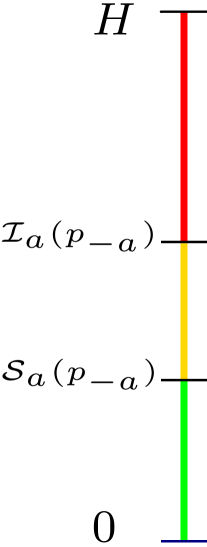
(a)

(b)

Figure 1: Mapping of Price Adjusting function

For all $p_{a}$ in red region, the functional value is lower than $p_{a}$ and equals $\mathcal{I}_{a}(p_{-a}).$ For all $p_{a}$ in green region, the functional value is higher than $p_{a}$ and equals $\mathcal{S}_{a}(p_{-a}).$ For all $p_{a}$ in yelllow region, the functional value is equal to $p_{a}$.

Figure $1(b)$ shows the case where $\mathcal{S}_{a}(p_{-a})>\mathcal{I}_{a}(p_{-a})$. All the prices $p_{a}$ would lie in blue region and $f_{a}(p_{a},p_{-a})=\frac{\mathcal{S}_{a}(p_{-a})+\mathcal{I}_{a}(p_{-a})}{2}$.

From now on, all the points satisfying condition $(I),~(II),~(III)$ and $(IV)$ are represented by red, yellow, green and blue colour respectively.

3 Results

The Tarski’s fixed point theorem states that if F is a monotone function on a non-empty complete lattice, the set of fixed points of F forms a non-empty complete lattice.
The price adjusting function defined above is monotonic (Proposition 1) and the set of fixed points is equal to the set of Walrasian equilibrium price vectors (Proposition 2). By Tarski’s fixed point theorem, it follows that the set of Walrasian equilibrium price vectors forms non-empty complete lattice.

We provide the proofs of Propositions 1 and 2 below.

Proposition 1.

$\mathbf{f}(\mathbf{p})$ is a monotonic function.

Proof.

Suppose $\mathbf{p}\leq\mathbf{q}$. We show that for all $a\in M,$ $f_{a}(\mathbf{p})\leq f_{a}(\mathbf{q})$.

We start by proving useful lemmas.

Lemma 1.

For $\mathbf{p}\leq\mathbf{q},$ we have $\mathcal{S}_{a}(p_{-a})\leq\mathcal{S}_{a}(q_{-a})$ and $\mathcal{I}_{a}(p_{-a})\leq\mathcal{I}_{a}(q_{-a})$.

Proof.

Suppose $\mathbf{p}\leq\mathbf{q}.$ Let $h_{a}\in\{h_{a}:\textrm{ no object is overdemanded at }(h_{a},h_{-a})\textrm{ where }h_{a}\geq\sup~\mathcal{O}_{a}(p_{-a}),h_{-a}\geq q_{-a}\}$. Note that $h_{a}\geq\sup~\mathcal{O}_{a}(q_{-a})\geq\sup\mathcal{O}_{a}(p_{-a})$, where last inequality follows from monotonicity of $\sup~\mathcal{O}_{a}.$ Also, $h_{-a}\geq q_{-a}\geq p_{-a}$, where the last inequality follows from the fact that $\mathbf{p}\leq\mathbf{q}.$ This implies $h_{a}\in\{h_{a}:\textrm{ no object is overdemanded at }(h_{a},h_{-a})\textrm{ where }h_{a}\geq\sup~\mathcal{O}_{a}(h_{-a}),h_{-a}\geq p_{-a}\}.$

Thus, we have

$$\{h_{a}:\textrm{ no object is overdemanded at }(h_{a},h_{-a})\textrm{ where }h_{a}\geq\sup~\mathcal{O}_{a}(p_{-a}),h_{-a}\geq q_{-a}\}$$

$$\subseteq\{h_{a}:\textrm{ no object is overdemanded at }(h_{a},h_{-a})\textrm{ where }h_{a}\geq\sup~\mathcal{O}_{a}(h_{-a}),h_{-a}\geq p_{-a}\}$$

$$\Rightarrow \inf~\{h_{a}:\textrm{ no object is overdemanded at }(h_{a},h_{-a})\textrm{ where }h_{a}\geq\sup~\mathcal{O}_{a}(p_{-a}),h_{-a}\geq q_{-a}\}\equiv\mathcal{S}_{a}(q_{-a})$$

$$\geq\inf~\{h_{a}:\textrm{ no object is overdemanded at }(h_{a},h_{-a})\textrm{ where }h_{a}\geq\sup~\mathcal{O}_{a}(p_{-a}),h_{-a}\geq p_{-a}\}\equiv\mathcal{S}_{a}(p_{-a}).$$

Analogously, we can show that $\mathcal{I}_{a}(p_{-a})\leq\mathcal{I}_{a}(q_{-a}).$ ∎

Lemma 2.

For all $\ell_{\leq}h_{a}$, for all $\ell_{-a}$, we have $f_{a}(\ell_{,}\ell_{-a})\leq f_{a}(h_{a},\ell_{-a}).$

(a)

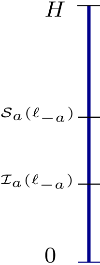
(b)

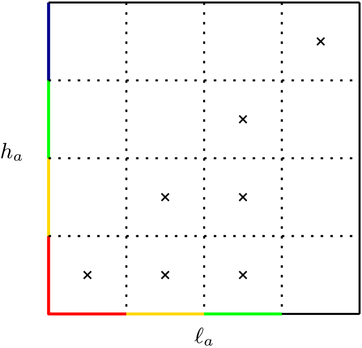
(c)

Figure 2: Coloured possibility matrix, given $\ell_{-a}$

Proof.

Fix $\ell_{-a}.$ This would fix $\mathcal{I}_{a}$ and $\mathcal{S}_{a}$ at $\ell_{-a}.$

We start by introducing a coloured matrix. The matrix reflects the possibility of $h_{a}$ and $\ell_{a}$ lying in a particular region. The $x-axis$ is $\ell_{a}$ and $y-axis$ is $h_{a}$. The cell in y coloured row and x coloured column would reflect if there is a possibility that $h_{a}$ lies in x coloured region and $\ell_{a}$ lies in y coloured region. Since $\ell_{a}\leq h_{a}$, the only possible cases are those marked with a cross.

Now we argue that $f_{a}(\ell_{a},\ell_{-a})\leq f_{a}(h_{a},\ell_{-a})$.

If $\ell_{a}$ lies in green region, $f_{a}(\ell_{a},\ell_{-a})=\mathcal{S}_{a}(\ell_{-a})$.  $h_{a}$ can lie in any of the region and $f_{a}(h_{a},\ell_{-a})\geq\mathcal{S}_{a}(\ell_{-a}).$

If $\ell_{a}$ lies in yellow region, $f_{a}(\ell_{a},\ell_{-a})=\ell_{a}.$  $h_{a}$ can lie in yellow region or red region. This gives $f_{a}(h_{a},\ell_{-a})\geq\min\{\mathcal{I}_{a}(\ell_{-a}),h_{a}\}\geq\ell_{a},$ where the former inequality follows from definition of $\mathbf{p}$ and the latter inequality follows from the fact that $h_{a}\geq\ell_{a}$ and $\ell_{a}$ lies in yellow region.

If $\ell_{a}$ lies in red region, $f_{a}(\ell_{a},h_{-a})=\mathcal{I}_{a}(\ell_{-a})$.  $h_{a}$ can lie in red region only. This gives $f_{a}(h_{a},\ell_{-a})=\mathcal{I}_{a}(\ell_{-a})$.

If $\ell_{a}$ lies in blue region, $f_{a}(\ell_{a},\ell_{-a})=\frac{\mathcal{S}_{a}(\ell_{-a})+\mathcal{I}_{a}(\ell_{-a})}{2}$. Also, $h_{a}$ lie in blue region, implying that $f_{a}(h_{a},\ell_{-a})=\frac{\mathcal{S}_{a}(\ell_{-a})+\mathcal{I}_{a}(\ell_{-a})}{2}.$

Thus, in all cases, $f_{a}(\ell_{a},\ell_{-a})\leq f_{a}(h_{a},\ell_{-a}).$ ∎

Lemma 2 has shown monotonicity in the first argument. Now we show monotonicity in other arguments, i.e. $f_{a}(p_{a},p_{-a})\leq f_{a}(p_{a},q_{-a})$. Since $p_{-a}\leq q_{-a},$ by Lemma 1, we get the possibility matrix as the following:

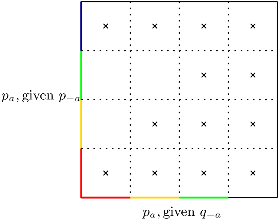
Figure 3: Coloured possibility matrix, given $p_{-a}$ and $q_{-a}$

Case 1. $p_{a}$ lies in blue region for $p_{-a}$.

We have $f_{a}(p_{a},p_{-a})=\frac{\mathcal{S}_{a}(p_{-a})+\mathcal{I}_{a}(p_{-a})}{2}.$ If $p_{a}$ is blue region for $q_{-a}$ as well, then $f_{a}(p_{a},q_{-a})=\frac{\mathcal{S}_{a}(q_{-a})+\mathcal{I}_{a}(q_{-a})}{2}\geq\frac{\mathcal{S}_{a}(p_{-a})+\mathcal{I}_{a}(p_{-a})}{2}=f_{a}(p_{a},p_{-a}),$ where inequality follows from Lemma 1. If $p_{a}$ not in blue region for $q_{-a}$, then $f_{a}(p_{a},q_{-a})\geq\mathcal{S}_{a}(q_{-a})\geq\mathcal{S}_{a}(p_{-a})\geq\frac{\mathcal{S}_{a}(p_{-a})+\mathcal{I}_{a}(p_{-a})}{2}=f_{a}(p_{a},p_{-a}),$ where the first inequality follows from definition of $f_{a}$,  second inequality follows from lemma 1 and third inequality follows from the fact that $\mathcal{S}_{a}(p_{-a})\geq\mathcal{I}_{a}(p_{-a}).$

Case 2. $p_{a}$ lies in blue region for $q_{-a}.$

We have $f_{a}(p_{a},q_{-a})=\frac{\mathcal{S}_{a}(q_{-a})+\mathcal{I}_{a}(q_{-a})}{2}.$ $f_{a}(p_{a},p_{-a})\leq\mathcal{I}_{a}(p_{-a})\leq\mathcal{I}_{a}(q_{-a})\leq\frac{\mathcal{S}_{a}(q_{-a})+\mathcal{I}_{a}(q_{-a})}{2}=f_{a}(p_{a},q_{-a})$, where the second inequality follows from Lemma 1 and the third inequality follows from the fact that $\mathcal{S}_{a}(q_{-a})>\mathcal{I}_{a}(q_{-a}).$

Notice that in reduced matrix without blue region, one just needs to show the inequality for diagonal. In lower triangular matrix, it is trivial from the mapping that the inequality wold be satisfied.

On the diagonal, the value of $(f_{a}(p_{a},p_{-a}),f_{a}(p_{a},q_{-a}))$ is $(\mathcal{I}_{a}(p_{-a}),\mathcal{I}_{a}(q_{-a})),~(p_{a},p_{a})$ and $(\mathcal{S}_{a}(p_{-a}),\mathcal{S}_{a}(q_{-a}))$ for red, yellow and green region respectively. By lemma 1, for all these possibilities, we have $f_{a}(p_{a},p_{-a})\leq f_{a}(p_{a},q_{-a})$.

Thus, we have established that $f_{a}(p_{a},p_{-a})\leq f_{a}(p_{a},q_{-a}).$ This combined with Lemma 2 gives $f_{a}(p_{a},p_{-a})\leq f_{a}(q_{a},q_{-a}).$ ∎

Proposition 2.

The following statements are equivalent:

1. $\mathbf{p}$ is fixed point of $\mathbf{f}.$

2. $\mathbf{p}$ is Walrasian price vector.

Proof.

Necessity: Suppose $\mathbf{p}$ is a Walrasian equilibrium. We would show that $\mathbf{f}(\mathbf{p})=\mathbf{p}$.
Note that since $\mathbf{p}$ is Walrasian equilibrium, no object $a\in M$ will be minimally underdemanded or overdemanded.
Fix an arbitrary object $a\in M$. We would argue that $\mathcal{I}_{a}(p_{-a})\geq p_{a}\geq\mathcal{S}_{a}(p_{-a})$.
We have $\mathcal{I}_{a}(p_{-a})\geq\inf\mathcal{U}_{a}(p_{-a})\geq p_{a}$, where the former inequality follows by definition of $\mathcal{I}_{a}$ and the latter inequality follows from the fact that no object is minimally underdemanded.

We show that $\mathcal{S}_{a}(p_{-a})\leq p_{a}$. Suppose not for contradiction. Also note that $p_{a}\geq\sup~\mathcal{O}_{a}(p_{-a})$ follows from the fact that no good is overdemanded. Combining the last two inequalities, we get $\mathcal{S}_{a}(p_{-a})>p_{a}\geq\sup~\mathcal{O}_{a}(p_{-a})$. By definition of $\mathcal{S}_{a}$, this implies some object was minimally overdemanded at $(p_{a},p_{-a}).$ A contradiction.

Thus, we have $\mathcal{I}_{a}(p_{-a})\geq p_{a}\geq\mathcal{S}_{a}(p_{-a})$. By definition of $\mathbf{f}$, $f_{a}(\mathbf{p})=p_{a}.$ Since, for all $a\in M$, $f_{a}(\mathbf{p})=p_{a}$, we have $\mathbf{f}(\mathbf{p})=\mathbf{p}.$
Sufficiency: Suppose $\mathbf{p}$ is a fixed point. Note that by definition, $\mathcal{I}_{a}(p_{-a})\geq\inf~\mathcal{U}_{a}(p_{-a})$ and $\mathcal{S}_{a}(p_{-a})\geq\sup~\mathcal{O}_{a}(p_{-a})$.

We will use the characterization of WE price vector in Theorem 1 of Mishra and Talman (2010), to show that $\mathbf{p}$ is Walrasian equilibrium price vector. The theorem is stated below.

Theorem.

A price vector $\mathbf{p}$ is a WE price vector if and only if no set of goods is overdemanded and no set of goods is underdemanded at $\mathbf{p}.$

We first show that no set is overdemanded at price $\mathbf{p}$. Suppose for contradiction that at $\mathbf{p}$, there exists an overdemanded set $S$. Let $a\in S$ is minimally overdemanded at $\mathbf{p}$.

Now we argue that $\mathcal{S}_{a}(p_{-a})>p_{a}.$ If for all $x\in S$, $h_{x}\in[p_{x},p_{x}+\epsilon]$ where $\epsilon\rightarrow 0$ and for all $x\notin S$, $h_{x}=p_{x}$, then the set $S$ will be overdemanded at $\mathbf{h}$. As a result, $\mathcal{S}_{a}(p_{-a})>p_{a}$.

Thus, only condition $(III)$ or $(IV)$ could hold true. By condition $(III)$, $f_{a}(\mathbf{p})=\mathcal{S}_{a}(p_{-a})>p_{a}$. A contradiction to the assumption that $\mathbf{p}$ is fixed point. Thus, the only possibility that we are left with is that $f_{a}(\mathbf{p})=\frac{\mathcal{S}_{a}(p_{-a})+\mathcal{I}_{a}(p_{-a})}{2}$. But $f_{a}(\mathbf{p})=p_{a}=\frac{\mathcal{S}_{a}(p_{-a})+\mathcal{I}_{a}(p_{-a})}{2}>\sup~\mathcal{O}(p_{-a})$. A contradicton to our assumption that $a$ is minimally overdemanded.

Thus, no set is overdemanded at $\mathbf{p}$.

Now we show that no set is overdemanded at $\mathbf{p}.$ Suppose for contradiction that set $T$ is overdemanded at $\mathbf{p}.$ Let $b\in T$ be the minimally underdemanded good. For all $x\in T$, if $h_{x}\in[p_{x}-\epsilon,p_{x}]$  where $\epsilon\rightarrow 0$ , and for all $x\notin T$, $h_{x}=p_{x}$, the set $T$ will be underdemanded. Thus, $\mathcal{I}(p_{-b})<p_{b}$.

Thus, condition $(II)$ or $(III)$ cannot be satisfied. If condition $(I)$ is satisfied, then $f_{b}(\mathbf{p})=\mathcal{I}(p_{-b})<p_{b}.$ A contradiction.

Thus, we are left with the case where $f_{b}(\mathbf{p})=\frac{\mathcal{S}_{b}(p_{-b})+\mathcal{I}_{b}(p_{-b})}{2}=p_{b}$. This implies that $\mathcal{S}_{b}(p_{-b})>p_{b}\geq\inf~\mathcal{U}_{b}(p_{-b})\geq\sup~\mathcal{O}_{b}(p_{-b})$, where first inequality follows from the fact that $p_{b}$ is average of $\mathcal{I}_{b}(p_{-b})$ and $\mathcal{S}_{b}(p_{-b})$ and $\mathcal{S}_{b}(p_{-b})>\mathcal{I}_{b}(p_{-b})$ . By definition of $\mathcal{S}_{b}(p_{-b})$, some object is minimally overdemanded at $(p_{b},p_{-b})$.

However we have already shown that no object is minimally overdemanded at fixed point, $\mathbf{p}$.

Thus, no set is overdemanded or underdemanded at $\mathbf{p}.$ By Theorem 1 of Mishra and Talman (2010), $\mathbf{p}$ is Walrasian equilibrium price vector.

∎

References

- Demange and Gale (1985) Demange, G. and D. Gale (1985): “The strategy structure of two-sided matching markets,” Econometrica: Journal of the Econometric Society, 873–888.
- Gale (1960) Gale, D. (1960): “Theory of linear Economic Models (New York, 1960),” .
- Mishra and Talman (2010) Mishra, D. and D. Talman (2010): “Characterization of the Walrasian equilibria of the assignment model,” Journal of Mathematical Economics, 46, 6–20.
- Quinzii (1984) Quinzii, M. (1984): “Core and competitive equilibria with indivisibilities,” International Journal of Game Theory, 13, 41–60.
- Shapley and Shubik (1971) Shapley, L. S. and M. Shubik (1971): “The assignment game I: The core,” International Journal of game theory, 1, 111–130.