Sensing Rate Optimization for Multi-Band Cooperative ISAC Systems

Abstract

Integrated sensing and communication (ISAC) has been recognized as one of the key technologies for future wireless networks, which potentially need to operate in multiple frequency bands to satisfy ever-increasing demands for both communication and sensing services. Motivated by this, we consider the sum sensing rate (SR) optimization for a cooperative ISAC system with linear precoding, where each base station (BS) works in a different frequency band. With this aim, we propose an optimization algorithm based on the semi-definite rank relaxation that introduces covariance matrices as optimization variables, and we apply the inner approximation (IA) method to deal with the nonconvexity of the resulting problem. Simulation results show that the proposed algorithm increases the SR by approximately 25 % and 40 % compared to the case of equal power distribution in a cooperative ISAC system with two and three BSs, respectively. Additionally, the algorithm converges in only a few iterations, while its most optimal implementation scenario is in the low power regime.

I Introduction

In addition to conventional communication services, future sixth-generation (6G) communication systems will need to provide high-precision sensing as a new necessary functionality underpinning different applications (e.g., augmented reality, digital twins). A promising technology for the implementation of this functionality with minimal additional resource usage is usually denoted as ISAC [1]. It refers to a design paradigm in which sensing and communication systems are integrated to efficiently utilize the shared spectrum and hardware resources, while offering mutual benefits. As such, ISAC is expected to be one of the key technologies in sixth-generation (6G) networks, which offers flexible trade-offs between the two functionalities across various use cases.

With the rise of high-data rate applications, wireless traffic demand is sharply increasing. This leads to spectrum congestion in the radio frequency (RF) band, which is insufficient for higher rate services. To meet these demands, all available spectrum, including sub-6 GHz, millimeter-wave (mmWave) and terraherz (THz) bands, must be fully utilized [2]. Furthermore, high-frequency technology also enables advanced sensing and localization with centimeter-level accuracy. Hence, frequency resource allocation is crucial for supporting both communication and sensing demands. Ultimately, future wireless networks will operate simultaneously in different frequency bands and will also need to possess cooperative capabilities. This fact motivates the development of cooperative ISAC systems that simultaneously operate in more than one frequency band.

Recent studies have explored ISAC in cooperative communication systems. A joint BS mode selection, transmit beamforming, and receive filter design for cooperative cell-free ISAC networks, where multiple BSs cooperatively serve communication users and detect targets, were studied in [3]. In [4], stochastic geometry was used to analyze scaling laws in cooperative ISAC networks, and it was shown that the sensing performance increases proportionally to the squared logarithm of the number of ISAC transceivers. In [5], a maximum likelihood (ML) framework for target localization was developed, deriving a cooperative position error bound (PEB) for the networked orthogonal time frequency space (OTFS)-based system which serves as a lower bound on positioning accuracy. Performance analysis and optimal power allocation in a cooperative ISAC system with a micro and a macro BS, where the micro BS performs sensing and acts as a full-duplex relay, were presented in [6].

Unlike previously studies on cooperative ISAC in a single frequency band, multi-band cooperative ISAC remains largely unexplored. In [7], a relatively complex method for fusion of orthogonal frequency division multiplexing (OFDM) sensing signals from different bands was proposed which achieved high-accuracy target localization, requiring dual-band processing at both BSs. A similar approach but for single-BS ISAC in [8] improved the sensing Cramer-Rao lower bound (CRLB) and communication mutual information, though it did not account for propagation loss differences between frequency bands.

Against this background, the contributions of this paper are listed as follows:

• We extend the mutual information (MI) framework developed in [9] to a multi-band cooperative ISAC system, where each BS operates in a different frequency band. To maximize the sum SR for this system, we formulate a joint optimization problem of the transmit precoding matrices. For this purpose, we adopt linear precoding. To maintain user fairness, each user has a guaranteed minimum CR.

• We solve the considered problem by employing the semi-definite rank relaxation method, which aims to find the covariance matrices of the corresponding precoding matrices. The IA method is applied to deal with the nonconvexity of the resulting problem.

• We demonstrate through simulations that the proposed algorithm increases the SR by approximately 25 % and 40 % compared to the case of equal power distribution in a cooperative ISAC system with two and three BSs, respectively. Additionally, the algorithm converges in a couple of iterations. Moreover, we show that the operating frequency and the distance from the sensing target have a significant impact on the SR. Lastly, we conclude that the most preferred application scenario for our proposed system model is in the low power regime.

Notation: Bold lower and upper case letters represent vectors and matrices, respectively. $\mathbf{I}_{x}$ is the unit matrix of a size $x\times x$. $\text{Tr}(\mathbf{X})$, $\text{vec}(\mathbf{X})$, $\det(\mathbf{X})$ and $\text{rank}(\mathbf{X})$ denote the trace, vectorization, determinant and rank of matrix $\mathbf{X}$, respectively. $\ln(\cdot)$ is the natural logarithm and $\otimes$ denotes the Kronecker product. $(\cdot)^{*}$ denotes complex-conjugate. $(\cdot)^{T}$ and $(\cdot)^{H}$ represent transpose and Hermitian transpose, respectively.

II System Model and Problem Formulation

We consider a system in which $B$ BSs, each being equipped with $N_{t}$ transmit and $N_{r}$ receive antennas, simultaneously serve $K$ communication users and perform target sensing. Each of the $B$ BSs operates on a different frequency band which is a typical scenario for 5G and beyond wireless networks. A given BS $b\in\mathcal{B}\triangleq\{1,2,\ldots,B\}$ operates at center frequency $f^{(b)}$, has a corresponding wavelength $\lambda^{(b)}$, and uses a bandwidth of $B^{(b)}$. Each user $k$ has $N_{k}$ antennas, where $k=1,2,\ldots,K$. Data symbols of unit average power are transmitted to all users over the period of $L$ time slots and are denoted as $\mathbf{S}^{(b)}=\bigl{[}(\mathbf{S}_{1}^{(b)})^{T},(\mathbf{S}_{2}^{(b)})^{T},\ldots,(\mathbf{S}_{K}^{(b)})^{T}\bigr{]}^{T}\in\mathbb{C}^{N_{\mathrm{tot}}\times L}$, where $\mathbf{S}_{k}^{(b)}\in\mathbb{C}^{N_{k}\times L}$ represents data symbols transmitted to user $k$ and $N_{\mathrm{tot}}=\sum_{k=1}^{K}N_{k}$. For asymptotically large $L$ , we can approximate

$$\mathbf{S}^{(b)}(\mathbf{S}^{(b)})^{H}\approx L\mathbf{I}_{N_{\mathrm{tot}}}.$$ (1)

To provide high-quality communication and sensing links, the transmit data steams for the $k$-th user are precoded with the matrix $\mathbf{W}_{k}^{(b)}\in\mathbb{C}^{N_{t}\times N_{k}}$. In low-frequency bands, a fully digital precoding matrix $\mathbf{W}_{k}^{(b)}$ is directly implemented, while in high-frequency bands, a hybrid precoding scheme is employed where $\mathbf{W}_{k}^{(b)}=\mathbf{W}_{RF,k}^{(b)}\mathbf{W}_{BB,k}^{(b)}$ with $\mathbf{W}_{BB,k}^{(b)}\in\mathbb{C}^{N_{k}\times N_{k}}$ as the fully digital baseband precoder and $\mathbf{W}_{RF,k}^{(b)}\in\mathbb{C}^{N_{t}\times N_{k}}$ as the analog precoder implemented using RF phase shifters. Hence, all of the elements of $\mathbf{W}_{RF,k}^{(b)}$ must satisfy

$$|\mathbf{W}_{RF,k}^{(b)}(i,j)|=1,\quad i=1,2,\ldots,N_{t},j=1,2,\ldots,N_{k}.$$ (2)

After precoding, the transmitted signal can be written as

$$\mathbf{X}^{(b)}=\mathbf{W}^{(b)}\mathbf{S}^{(b)}=\sum\nolimits_{k=1}^{K}\mathbf{W}_{k}^{(b)}\mathbf{S}_{k}^{(b)}\in\mathbb{C}^{N_{t}\times L}$$ (3)

where $\mathbf{W}^{(b)}=\bigl{[}\mathbf{W}_{1}^{(b)},\mathbf{W}_{2}^{(b)},\ldots,\mathbf{W}_{K}^{(b)}\bigr{]}\in\mathbb{C}^{N_{t}\times N_{\text{tot}}}$.

II-A Communication Model

For the frequency band $b$, the received signals of all users can be stacked to form a matrix $\mathbf{Y}_{C}^{(b)}$, given by

$$\mathbf{Y}_{C}^{(b)}=\mathbf{H}^{(b)}\mathbf{X}^{(b)}+\mathbf{N}^{(b)}\in\mathbb{C}^{N_{\mathrm{tot}}\times L}$$ (4)

where $\mathbf{H}^{(b)}=\bigl{[}\mathbf{H}_{1}^{(b)T},\mathbf{H}_{2}^{(b)T},\cdots,\mathbf{H}_{K}^{(b)T}\bigr{]}^{T}\in\mathbb{C}^{N_{\mathrm{tot}}\times N_{t}}$ with $\mathbf{H}_{k}^{(b)}\in\mathbb{C}^{N_{k}\times N_{t}}$ being the channel matrix between the $b$-th BS and the $k$-th user. $\mathbf{N}^{(b)}\in\mathbb{C}^{N_{\mathrm{tot}}\times L}$ is the noise matrix consisting of independent and identically distributed (i.i.d.) elements that are distributed according to $\mathcal{CN}(0,(\sigma^{(b)})^{2})$. Assuming a sparsely-scattered channel model, the channel matrix can be expressed as

$$\mathbf{H}_{k}^{(b)}=\sqrt{\frac{N_{t}N_{k}}{P^{(b)}}}\sum\nolimits_{p=1}^{P^{(b)}}\beta_{p,k}^{(b)}\mathbf{a}_{\mathrm{R}}(\theta_{p,k}^{(b)})\mathbf{a}_{\mathrm{T}}(\phi_{p,k}^{(b)})^{H}$$ (5)

where $P^{(b)}$ is the number of signal paths and $\beta_{p,k}^{(b)}$ is the gain of path $p$ which is distributed according to $\mathcal{CN}(0,F_{k}^{(b)})$. In the above, $F_{k}^{(b)}$ is the free space path loss, calculated as $F_{k}^{(b)}=(\lambda^{(b)}/4\pi d_{k}^{(b)})^{2}$, where $d_{k}^{(b)}$ is the distance between the BS $b$ and user $k$. Also, $\theta_{p,k}^{(b)}$ and $\phi_{p,k}^{(b)}$ denote the angle of arrival (AoA) and angle of departure (AoD) for the $p$-th path between the BS and user $k$. The transmit and receive antenna array responses are given by $\mathbf{a}_{\mathrm{T}}(\theta_{t}^{(b)})=\frac{1}{\sqrt{N_{t}}}[1,e^{j\frac{2\pi s_{t}^{(b)}}{\lambda^{(b)}}\sin\theta_{p,k}^{(b)}},\cdots,e^{j(N_{t}-1)\frac{2\pi s_{t}^{(b)}}{\lambda^{(b)}}\sin\theta_{p,k}^{(b)}}]^{T}$ and $\mathbf{a}_{\mathrm{R}}(\theta_{r}^{(b)})=\frac{1}{\sqrt{N_{k}}}[1,e^{j\frac{2\pi s_{k}^{(b)}}{\lambda^{(b)}}\sin\phi_{p,k}^{(b)}},\cdots,e^{j(N_{k}-1)\frac{2\pi s_{k}^{(b)}}{\lambda^{(b)}}\sin\phi_{p,k}^{(b)}}]^{T}$, respectively, where $s_{t}^{(b)}$ and $s_{k}^{(b)}$ are the spacing between the adjacent transmit and receive antennas, respectively.

For a single frequency band with bandwidth $B^{(b)}$, the achievable rate for user $k$ can be expressed as

$$\!\!\!\!\!\!R_{C,k}^{(b)}=B^{(b)}\ln\det\bigl{[}\mathbf{I}_{N_{k}}+\mathbf{H}_{k}^{(b)}\mathbf{W}_{k}^{(b)}\mathbf{W}_{k}^{(b)H}\mathbf{H}_{k}^{(b)H}\\ \!\!\!\!\!\!\times\!\!\bigl{(}\sum\nolimits_{i=1,i\neq k}^{K}\mathbf{H}_{k}^{(b)}\mathbf{W}_{i}^{(b)}\mathbf{W}_{i}^{(b)H}\mathbf{H}_{k}^{(b)H}+(\sigma^{(b)})^{2}\mathbf{I}_{N_{k}}\bigr{)}^{-1}\bigr{]}.$$ (6)

II-B Sensing Model

For target detection, each BS utilizes collocated transmit and receive antennas to perform monostatic sensing. We assume that the transmit and receive antennas at the same BS are separated and sufficiently isolated from one another, so that any self-interference can be ignored. Therefore, the AoD and AoA for each sensing signal are the same. If no scattering interference is present in the sensing channel, the echo signal is given by

$$\mathbf{Y}_{S}^{(b)}=\mathbf{G}^{(b)}\mathbf{X}^{(b)}+\mathbf{Z}^{(b)}=\mathbf{G}^{(b)}\mathbf{W}^{(b)}\mathbf{S}^{(b)}+\mathbf{Z}^{(b)}$$ (7)

where $\mathbf{G}^{(b)}\in\mathbb{C}^{N_{r}\times N_{t}}$ is the target response matrix and $\mathbf{Z}^{(b)}\in\mathbb{C}^{N_{r}\times L}$ is the noise matrix whose elements are distributed as $\mathcal{CN}(0,(\sigma^{(b)})^{2})$. This equation can be further reformulated as [9]

$$\mathbf{y}_{S}^{(b)}=\widetilde{\mathbf{W}}^{(b)}\mathbf{\widetilde{S}}^{(b)}\mathbf{g}^{(b)}+\mathbf{z}^{(b)}$$ (8)

where $\mathbf{\widetilde{S}}^{(b)}=\mathbf{I}_{N_{r}}\otimes(\mathbf{S}^{(b)})^{H}$, $\mathbf{\widetilde{W}}^{(b)}=\mathbf{I}_{N_{r}}\otimes(\mathbf{W}^{(b)})^{H}$, $\mathbf{y}_{S}^{(b)}=\text{vec}((\mathbf{Y}_{S}^{(b)})^{H})$, $\mathbf{g}^{(b)}=\text{vec}((\mathbf{G}^{(b)})^{H})$ and $\mathbf{z}^{(b)}=\text{vec}((\mathbf{Z}^{(b)})^{H})$.

For a point target, the response matrix and its covariance matrix are given by

$$\mathbf{G}^{(b)} =\alpha^{(b)}\sqrt{N_{t}N_{r}}\mathbf{a}_{\mathrm{R}}(\varphi{}^{(b)})\mathbf{a}_{\mathrm{T}}(\varphi{}^{(b)})^{H}$$ (9)

$$\mathbf{R}^{(b)} =\mathbb{E}\{\mathbf{g}^{(b)}\mathbf{g}^{(b)H}\}=\gamma N_{t}N_{r}(\mathbf{a}_{\mathrm{R}}(\varphi{}^{(b)})^{*}\otimes\mathbf{a}_{\mathrm{T}}(\varphi{}^{(b)}))$$

$$\quad\quad\times(\mathbf{a}_{\mathrm{R}}(\varphi{}^{(b)})^{*}\otimes\mathbf{a}_{\mathrm{T}}(\varphi{}^{(b)}))^{H}$$ (10)

where $\varphi{}^{(b)}$ is the sensing AoA/AoD, $\alpha^{(b)}$ is the reflection coefficient of the sensing channel gain, and $\gamma=\mathbb{E}\{\alpha^{(b)}\alpha^{(b)*}\}$. The standard deviation of $\alpha^{(b)}$ is $\sqrt{\beta_{\mathrm{RCS}}(\lambda^{(b)})^{2}/(4\pi)^{3}(d^{(b)})^{4})}$, where $d^{(b)}$ is the distance between the BS and sensing target, and $\beta_{\mathrm{RCS}}$ is the radar cross section (RCS) [10]. Since the proposed optimization algorithm is applicable for any RCS, we take $\beta_{\mathrm{RCS}}=1$ for ease of exposition. To ensure numerical stability, we normalize the communication channel and the target response matrices by the noise standard deviation, i.e., $\mathbf{\bar{H}}_{k}^{(b)}\leftarrow\mathbf{H}_{k}^{(b)}/\sigma^{(b)}$ and $\mathbf{\bar{G}}^{(b)}\leftarrow\mathbf{G}^{(b)}/\sigma^{(b)}$, which implies $\mathbf{\bar{R}}^{(b)}\leftarrow\mathbf{R}^{(b)}/(\sigma^{(b)})^{2}$.

For radar signal processing, both $\widetilde{\mathbf{W}}^{(b)}$ and $\mathbf{\widetilde{S}}^{(b)}$ are known to the receiver. Thus, the MI between $\mathbf{y}_{S}^{(b)}$ and $\mathbf{g}^{(b)}$ can be calculated as [9]

$$\mathcal{I}(\mathbf{y}_{S}^{(b)};\mathbf{g}^{(b)}|\widetilde{\mathbf{W}}^{(b)},\mathbf{\widetilde{S}}^{(b)})$$

$$=\mathcal{H}(\mathbf{y}_{S}^{(b)}|\widetilde{\mathbf{W}}^{(b)},\mathbf{\widetilde{S}}^{(b)})-\mathcal{H}(\mathbf{y}_{S}^{(b)};\mathbf{g}^{(b)}|\widetilde{\mathbf{W}}^{(b)},\mathbf{\widetilde{S}}^{(b)})$$

$$=\ln\det(L\widetilde{\mathbf{W}}^{(b)}\mathbf{\bar{R}}^{(b)}\widetilde{\mathbf{W}}^{(b)H}+\mathbf{I}_{N_{\mathrm{tot}}N_{r}}).$$ (11)

From an information-theoretic point of view, we adopt the SR as the performance metric of sensing, which is defined as the MI per unit time [11]. For target sensing at band $b$, the SR is given by

$$R_{S}^{(b)} =\frac{1}{L}B^{(b)}\mathcal{I}(\mathbf{y}_{S}^{(b)};\mathbf{g}^{(b)}|\widetilde{\mathbf{W}}^{(b)},\mathbf{\widetilde{S}}^{(b)})$$

$$=\frac{1}{L}B^{(b)}\ln\det(L\widetilde{\mathbf{W}}^{(b)}\mathbf{\bar{R}}^{(b)}\widetilde{\mathbf{W}}^{(b)H}+\mathbf{I}_{N_{\mathrm{tot}}N_{r}}).$$ (12)

Note that both the CR in (6) and the SR in (12) are expressed in nat/s for mathematical convenience.

II-C Problem Formulation

In this paper, we are interested in designing a cooperative ISAC system that maximizes the SR constrained by the total transmit power budget and the per-user CR requirements, leading to the following optimization problem:

​​$$\underset{\{\mathbf{W}_{k}^{(b)}\}}{\operatorname{max.}} \ \sum\nolimits_{b\in\mathcal{B}}R_{S}^{(b)}$$ (13a)

$$\operatorname{s.t.} \ \sum\nolimits_{b\in\mathcal{B}}\sum\nolimits_{k=1}^{K}\operatorname{Tr}(\mathbf{W}_{k}^{(b)}\mathbf{W}_{k}^{(b)H})\leq P_{\text{max}},$$ (13b)

$$\ \sum\nolimits_{b\in\mathcal{B}}R_{C,k}^{(b)}\geq r_{\min},\forall k$$ (13c)

where (13b) ensures the total transmit power does not exceed the maximum allowable power, and (13c) guarantees each user achieves at least the minimum required CR $r_{\min}$. Since we do not consider complex signal combining of the echo signals across different frequency bands, the sum SR serves as an appropriate objective function in (13).

III Proposed Solution

Since solving for $\{\mathbf{W}_{k}^{(b)}\}$ directly is challenging, we resort to the semi-definite rank relaxation method by introducing the covariance matrices $\mathbf{Q}_{k}^{(b)}=\mathbf{W}_{k}^{(b)}\mathbf{W}_{k}^{(b)H}$. As a result, the SR at band $b$ can be rewritten as

$$\!\!\!R_{S}^{(b)} =\tfrac{1}{L}B^{(b)}\ln\det(L\widetilde{\mathbf{W}}^{(b)}\mathbf{\bar{R}}^{(b)}\widetilde{\mathbf{W}}^{(b)H}+\mathbf{I}_{N_{\mathrm{tot}}N_{r}})$$

$$\!\!\!\!\!\!\!\!\!\!\!\!=\tfrac{1}{L}B^{(b)}\ln\det\bigl{[}L\bigl{(}\mathbf{I}_{N_{r}}\otimes\sum\nolimits_{k=1}^{K}\mathbf{Q}_{k}^{(b)}\bigr{)}\mathbf{\bar{R}}^{(b)}+\mathbf{I}_{N_{t}N_{r}}\bigr{]}$$ (14)

where we used the identities $\det(\mathbf{X}\mathbf{Y}+\mathbf{I}_{m})=\det(\mathbf{Y}\mathbf{X}+\mathbf{I}_{n})$, $(\mathbf{X}_{1}\mathbf{Y}_{1})\otimes(\mathbf{X}_{2}\mathbf{Y}_{2})=(\mathbf{X}_{1}\otimes\mathbf{X}_{2})(\mathbf{Y}_{1}\otimes\mathbf{Y}_{2})$ and (1). We remark that $R_{S}^{(b)}$ is jointly concave with all $\mathbf{Q}_{k}^{(b)}$, which makes the objective function in (13a) easier to handle. Similarly, the CR of user $k$ at band $b$ is given by

$$R_{C,k}^{(b)}=B^{(b)}\bigl{[}\ln\det(\mathbf{B}_{k}^{(b)}+\mathbf{\bar{H}}_{k}^{(b)}\mathbf{Q}_{k}^{(b)}\mathbf{\bar{H}}_{k}^{(b)H})\\ -\ln\det(\mathbf{B}_{k}^{(b)})\bigr{]}$$ (15)

where $\mathbf{B}_{k}^{(b)}=\sum_{j=1,j\neq k}^{K}\mathbf{\bar{H}}_{k}^{(b)}\mathbf{Q}_{j}^{(b)}\mathbf{\bar{H}}_{k}^{(b)H}+\mathbf{I}_{N_{k}}$. Therefore, the original optimization problem (13) can be equivalently reformulated as

​​$$\underset{\mathbf{Q}_{k}^{(b)}\in\mathcal{Q}}{\operatorname{max.}} \ f(\{\mathbf{Q}_{k}^{(b)}\})\triangleq\sum\nolimits_{b\in\mathcal{B}}R_{S}^{(b)}$$ (16a)

$$\operatorname{s.t.} \ \sum\nolimits_{b\in\mathcal{B}}R_{C,k}^{(b)}\geq r_{\min},\forall k$$ (16b)

$$\ \mathrm{rank}(\mathbf{Q}_{k}^{(b)})=N_{k}$$ (16c)

where $\mathcal{Q}\triangleq\{\mathbf{Q}_{k}^{(b)}\,|\,\sum\nolimits_{b\in\mathcal{B}}\sum\nolimits_{k=1}^{K}\operatorname{Tr}(\mathbf{Q}_{k}^{(b)})\leq P_{\text{max}}\}$ and (16c) ensures that $\mathbf{W}_{k}^{(b)}$ can be exactly computed from $\mathbf{Q}_{k}^{(b)}$.

It is straightforward to see that the primary challenges in solving (16) are the non-convex constraints (16b) and (16c). To overcome these, we first implement rank relaxation and drop the rank constraint (16c). Next, (16) we apply the IA method to solve the resulting problem [12]. To this end, a concave lower bound for $R_{C,k}^{(b)}$ is required. We note that $R_{C,k}^{(b)}$ is in fact the difference of two concave functions. Thus, a lower bound can be easily obtained by linearizing the term $\ln\det(\mathbf{B}_{k}^{(b)})$. Let $\mathbf{Q}_{k}^{(b),n}$ and $\mathbf{B}_{k}^{(b),n}$ be the values of $\mathbf{Q}_{k}^{(b)}$ and $\mathbf{B}_{k}^{(b)}$ in the $n$-th iteration, respectively. Then the following inequality holds:

$$\ln\det(\mathbf{B}_{k}^{(b)})\leq\ln\det(\mathbf{B}_{k}^{(b),n})+\\ \sum\nolimits_{i=1,i\neq k}^{K}\operatorname{Tr}\bigl{(}\mathbf{H}_{k}^{(b)H}(\mathbf{B}_{k}^{(b),n})^{-1}\mathbf{H}_{k}^{(b)}(\mathbf{Q}_{i}^{(b)}-\mathbf{Q}_{i}^{(b),n})\bigr{)}$$ (17)

which is due to the concavity of the $\ln\det()$ function.

Substituting (17) into (15), a lower bound on the CR is given by

$$R_{C,k}^{(b)}\geq\bar{R}_{C,k}^{(b)}=B^{(b)}\Bigl{[}\ln\det(\mathbf{B}_{k}^{(b)}+\mathbf{\bar{H}}_{k}^{(b)}\mathbf{Q}_{k}^{(b)}\mathbf{\bar{H}}_{k}^{(b)H})$$

$$-\ln\det(\mathbf{B}_{k}^{(b),n})$$

$$-\sum_{i=1,i\neq k}^{K}\operatorname{Tr}\bigl{(}\mathbf{\bar{H}}_{k}^{(b)H}(\mathbf{B}_{k}^{(b),n})^{-1}\mathbf{\bar{H}}_{k}^{(b)}(\mathbf{Q}_{i}^{(b)}-\mathbf{Q}_{i}^{(b),n})\bigr{)}\Bigr{]}.$$ (18)

which is jointly concave with respect to all $\mathbf{Q}_{k}^{(b)}$. Utilizing (18), $\mathbf{Q}_{i}^{(b),n+1}$ is obtained as the solution to the following convex problem:

​​$$\underset{\mathbf{Q}_{k}^{(b)}\in\mathcal{Q}}{\operatorname{max.}} \quad f(\{\mathbf{Q}_{k}\})$$ (19a)

$$\operatorname{s.t.} \quad\sum\nolimits_{b\in\mathcal{B}}\bar{R}_{C,k}^{(b)}\geq r_{\min},\forall k,$$ (19b)

Initialization

The proposed method requires a feasible point to start, which is not trivial to obtain due to the nonconvexity of $R_{C,k}^{(b)}$. To overcome this issue, we consider the following regularized problem of (19):

​​$$\underset{\mathbf{Q}_{k}^{(b)}\in\mathcal{Q},s_{k}\geq 0}{\operatorname{max.}} \quad f(\{\mathbf{Q}_{k}\})-\rho\sum_{k=1}^{K}s_{k}$$ (20a)

$$\operatorname{s.t.} \quad\sum\nolimits_{b\in\mathcal{B}}\bar{R}_{C,k}^{(b)}+s_{k}\geq r_{\min},\forall k$$ (20b)

where $s_{k}\geq 0$ ($k=1,2,\dots,K$) are slack variables, and $\rho>0$ is the regularization factor. It is straightforward to see that (20) is always feasible for any initial choice of $\mathbf{Q}_{i}^{(b),0}$. Due to the regularization term, the slack variables are gradually forced to zero as the iterations progress. Once this happens, the obtained $\mathbf{Q}_{k}^{(b)}$ is feasible to (16), and thus, can be used to initialize the proposed iterative optimization method. 1 outlines the overall proposed method.

Input: $\mathbf{Q}_{k}^{(b),0}$ (randomly generated), $\rho\geq 0$, $m\leftarrow 0$

1

2repeat // find a feasible point

3  

4  Solve (20) to obtain $\mathbf{Q}_{k}^{(b),m+1}$ and increase $m$: $m\leftarrow m+1$

5  

6   until  $\forall s_{k}<\epsilon$

7  Reset $\mathbf{Q}_{k}^{(b),0}\leftarrow\mathbf{Q}_{k}^{(b),m+1}$ and set $n\leftarrow 0$

8  repeat

9    

10    Solve (19) to obtain $\mathbf{Q}_{k}^{(b),n+1}$ and increase $n$: $n\leftarrow n+1$

11    

12     until convergence

    Output: $\mathbf{Q}_{k}^{(b),\ast}=\mathbf{Q}_{k}^{(b),n+1},k=1,2,\ldots,K$

Algorithm 1 Optimization of the covariance matrices.

Remark 1.

After the optimization is complete, the appropriate precoding matrices $\mathbf{W}_{k}^{(b)}$ can be obtained from the covariance matrices $\mathbf{Q}_{k}^{(b),\ast}$. If $\text{rank}(\mathbf{Q}_{k}^{(b),\ast})=N_{k}$, then $\mathbf{W}_{k}^{(b)}$ can be obtained exactly from $\mathbf{Q}_{k}^{(b),\ast}$ by eigenvalue decomposition (EVD). If not, then randomization methods introduced in [13] are applied to find $\mathbf{W}_{k}^{(b)}$. However, in our extensive numerical experiments, the condition $\text{rank}(\mathbf{Q}_{k}^{(b),\ast})=N_{k}$ is always met, and thus, randomization is not neccessary. This strongly indicates the potential existence of an analytical proof for this empirical observation. Pursuing such a proof is beyond the scope of this work, and we leave this interesting open problem for future research. For the high-frequency bands, $\mathbf{W}_{BB,k}^{(b)}$ and $\mathbf{W}_{RF,k}^{(b)}$ are obtained from $\mathbf{W}_{k}^{(b)}$ by applying orthogonal matching pursuit (OMP) [14, Algorithm 1].

Convergence Analysis

The convergence analysis of the proposed method closely follows the arguments presented in [12]. It is easy to see that the inequality in (18) is tight when $\mathbf{Q}_{i}^{(b)}=\mathbf{Q}_{i}^{(b),n}$, $i=1,2,\ldots,K$, which implies that $\{\mathbf{Q}_{i}^{(b),n}\}$ is feasible to (19). Since $\{\mathbf{Q}_{i}^{(b),n+1}\}$ is the global solution to (19), it follows that $f(\{\mathbf{Q}_{k}^{n+1}\})\geq f(\{\mathbf{Q}_{k}^{n}\})$, i.e., the objective sequence $f(\{\mathbf{Q}_{k}^{n}\})$ is nondecreasing. Assuming that the feasible set of (16) is nonempty, then the sequence $f(\{\mathbf{Q}_{k}^{n}\})$ is bounded above, and is thus convergent since the feasible set is compact.

We remark that the objective function in (20a) strikes a balance between maximizing the SR and ensuring the feasibility of (19). Thus, once a feasible starting point is achieved (cf. Line 1 of 1), it is also a good starting point. This, in turn, accelerates the convergence of the main iterative procedure, enabling the algorithm to terminate within only a few iterations, as shall be demonstrated in the next section.

IV Simulation Results

In this section, we evaluate the SR of the proposed algorithm for a cooperative ISAC system through Monte Carlo simulations and compare it with three benchmark schemes. In the first benchmark scheme, which is denoted as Eq-Pow-Split, the total power budget is uniformly distributed among all BSs, i.e., the power budget of each BS is $P_{\text{max}}/B$. In the other three benchmark schemes, which are denoted as BS1 Only, BS2 Only and BS3 Only, only the BS1, BS2 and BS3 are active, respectively.

In the simulation setup, we consider three frequency bands $f^{(1)}=6\,\text{GHz}$ ($\lambda^{(1)}=5\,\text{cm}$), $f^{(2)}=26\,\text{GHz}$ ($\lambda^{(2)}\approx 1.15\,\text{cm}$), $f^{(3)}=26.5\,\text{GHz}$ ($\lambda^{(3)}\approx 1.13\,\text{cm}$) with the corresponding bandwidths $B^{(1)}=1\,\text{MHz}$ and $B^{(2)}=B^{(3)}=4\,\text{MHz}$. That is, BS1 operates in the low-frequency band, while BS2 and BS3 operate in the high-frequency bands. The number of propagation paths is $P^{(1)}=8$ and $P^{(2)}=P^{(3)}=4$, while the minimum communication rate requirement is $r_{\min}=100\,\mathrm{kbit/s}$. Other parameters are set as $N_{t}=8$, $N_{r}=2$, $N_{k}=2$, $L=30$, $\rho=1$, $\epsilon=10^{-5}$. The noise power is calculated according to $(\sigma^{(b)})^{2}=k_{B}TB^{(b)}F$, where $k_{B}=1.381\times 10^{-23}$ is the Boltzmann constant, $T=290\,\text{K}$ is the standard temperature, and $F=7.94$ (i.e., $9\,\text{dB}$) is the noise figure of the receiver. The midpoints of the transmit and the receive uniform linear arrays for BS1, BS2, and BS3 are at $(0,5\,\mathrm{m},0)$, $(0,5\,\mathrm{m},300\,\mathrm{m})$, and $(210\,\text{$\mathrm{m}$},5\,\mathrm{m},-80\,\text{$\mathrm{m}$})$, respectively, with ULAs at BS1 and BS2 oriented along the $z$-axis, and at BS3 along the $x$-axis. The midpoint of the $k$-th user’s ULA is $(25\,\mathrm{m},1.5\,\mathrm{m},z_{k})$, where $z_{k}$ is uniformly distributed in $[25\,\mathrm{m},275\,\mathrm{m}]$, while the point target is located at $(-25\,\mathrm{m},1\,\mathrm{m},z_{t})$, where $z_{t}$ follows the same uniform distribution as $z_{k}$. The inter-antenna spacing for each BS is half of the wavelength of its operating frequency, while for users, this spacing is $\lambda^{(1)}/2$ to avoid antenna coupling. The AoA ($\theta_{p,k}^{(b)}$) and AoD ($\phi_{p,k}^{(b)}$) are uniformly sampled from $[-\pi/2,\pi/2]$. The CVX tool with MOSEK as the internal software package are used to implement 1. The initial values of the covariance matrices are randomly generated while satisfying the total power budget. 1 terminates once the relative change of the SR is less than $10^{-3}$. Moreover, the SR is measured in bits per second (bit/s) and averaged over 500 independent channel realizations.

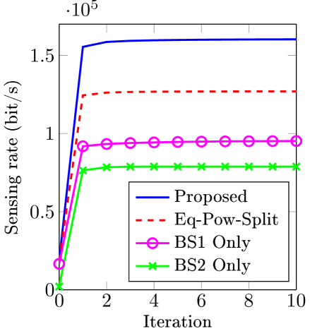
(a) For two BSs.

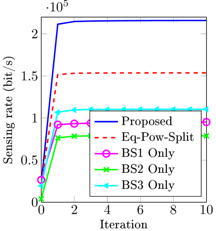
(b) For three BSs.

Figure 1: Convergence of the proposed algorithm and benchmark schemes for different numbers of BSs.

In Fig. 1, we present the convergence behavior of the proposed algorithm and benchmark schemes for an ISAC cooperative system with two and three BSs. In general, all schemes require only a few iterations to fully converge after a feasible point is found. Due to its ability to optimally distribute power among the BSs, the proposed algorithm achieves the largest SR, outperforming the Eq-Pow-Split scheme by approximately 25 % and 40 % in cooperative ISAC systems with two and three BSs, respectively. Moreover, Eq-Pow-Split provides the best sensing performance among the benchmark schemes, since it combines the ISAC capabilities of multiple BSs. Regarding benchmark schemes with only one active BS, BS3 Only achieves the highest individual SR, although it operates at a higher frequency than the other BSs. This can be attributed to the fact that the BS3 is in most cases closer to the sensing target, particularly when the target is equidistant from the first two BSs. These results indicate that, besides the operating frequency, the distance from the sensing target is another key factor that determines the SR in ISAC cooperative systems. In general, we can observe that the proposed algorithm for cooperative ISAC communications generally offers a substantially larger SR, compared to benchmark schemes with only one active BS. The only exception is in scenarios where the sensing target is located very close to a single BS, which makes the cooperation gain negligible. Moreover, in our simulations, $\text{rank}(\mathbf{Q}_{k}^{(b),\ast})$ is always equal to $N_{k}$ for $k=1,2,\ldots,K$, which implies that dropping the rank constraint does not affect the optimality of (16).

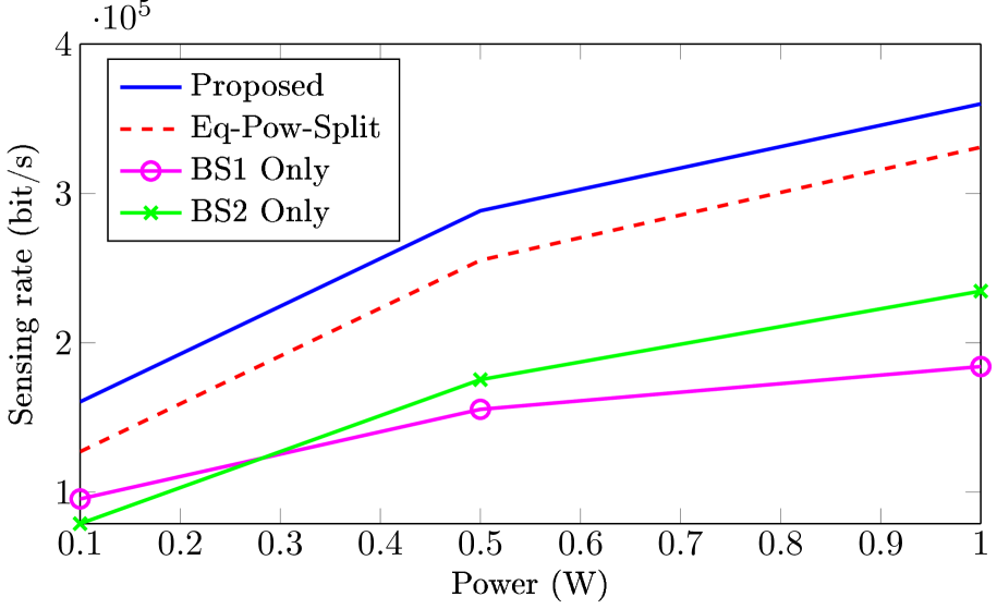
Figure 2: SR versus transmit power.

The variation of the SR with the transmit power with two BSs is shown in Fig. 2. Similar results were obtained for in the case of three BSs. As expected, the SRs of all schemes increase logarithmically with the transmit power. The advantage of using the cooperative ISAC capabilities of both BSs, rather than relying on a single BS, becomes more apparent with higher transmit power. The proposed scheme consistently achieves a larger SR than Eq-Pow-Split, but the performance gap remains approximately constant across different power levels. This suggests that the proposed scheme is particularly beneficial in the low to medium transmit power range, while Eq-Pow-Split serves as a reasonable sub-optimal solution in the high transmit power regime. Regarding the benchmark schemes with only one active BS, BS1 Only achieves a larger SR in the lower transmit power region, while the opposite is true in the higher transmit power region. This is due to the fact that at higher transmit power levels, the higher propagation losses associated with higher-frequency bands (e.g., BS2) can be compensated by increased channel directivity, which enhances sensing performance.

V Conclusion

In this paper, we have studied the sum SR maximization in a cooperative ISAC system with linear precoding, where each BS operates in a different frequency band. With that aim, we developed an algorithm based on the semi-definite rank relaxation method by introducing the covariance matrices of the appropriate precoding matrices as optimization variables and utilized the IA method to deal with the nonconvexity of the resulting problem. Simulation results show that the proposed algorithm increases the SR by approximately 25 % and 40 % compared to the case of equal power distribution in a cooperative ISAC system with two and three BSs, respectively. Additionally, the algorithm converges in a couple of iterations. Lastly, we conclude that the proposed method is most effective in the low transmit power regime, where power-efficient cooperative sensing and communication are essential.

References

- [1] F. Liu et al., “Integrated sensing and communications: Toward dual-functional wireless networks for 6G and beyond,” IEEE J. Sel. Areas Commun, vol. 40, no. 6, pp. 1728–1767, 2022.
- [2] C.-X. Wang et al., “On the road to 6G: Visions, requirements, key technologies, and testbeds,” IEEE Commun. Surv. Tutor., vol. 25, no. 2, pp. 905–974, 2023.
- [3] S. Liu et al., “Cooperative cell-free ISAC networks: Joint BS mode selection and beamforming design,” in Proc. IEEE WCNC, 2024, pp. 1–6.
- [4] K. Meng et al., “Cooperative ISAC networks: Performance analysis, scaling laws and optimization,” IEEE Trans. Wireless Commun., vol. 24, no. 2, pp. 877–892, 2025.
- [5] L. Pucci et al., “Cooperative maximum likelihood target position estimation for MIMO-ISAC networks,” arXiv preprint arXiv:2411.05187, 2024.
- [6] M. Liu et al., “Performance analysis and power allocation for cooperative ISAC networks,” IEEE Internet Things J., vol. 10, no. 7, pp. 6336–6351, 2022.
- [7] H. Liu et al., “Target localization with macro and micro base stations cooperative sensing,” arXiv preprint arXiv:2405.02873, 2024.
- [8] ——, “Carrier aggregation enabled MIMO-OFDM integrated sensing and communication,” arXiv preprint arXiv:2405.10606, 2024.
- [9] J. Li et al., “A framework for mutual information-based MIMO integrated sensing and communication beamforming design,” IEEE Trans. Veh. Technol., vol. 73, no. 6, pp. 8352–8366, 2024.
- [10] F. Dong et al., “Sensing as a service in 6G perceptive networks: A unified framework for ISAC resource allocation,” IEEE Trans. Wireless Commun., vol. 22, no. 5, pp. 3522–3536, 2022.
- [11] C. Ouyang et al., “MIMO-ISAC: Performance analysis and rate region characterization,” IEEE Wireless Commun. Lett., vol. 12, no. 4, pp. 669–673, 2023.
- [12] B. R. Marks and G. P. Wright, “A general inner approximation algorithm for nonconvex mathematical programs,” Operations Research, vol. 26, no. 4, pp. 681–683, 1978.
- [13] N. D. Sidiropoulos et al., “Transmit beamforming for physical-layer multicasting,” IEEE Trans. Signal Process., vol. 54, no. 6, pp. 2239–2251, 2006.
- [14] O. El Ayach et al., “Spatially sparse precoding in millimeter wave MIMO systems,” IEEE Trans. Wireless Commun., vol. 13, no. 3, pp. 1499–1513, 2014.